Study of polarization for even-denominator fractional quantum Hall states in SU(4) Graphene

Abstract

We have focussed to study the even-denominator fractional quantum Hall (EDFQH) states observed in monolayer graphene. In this letter, we have studied polarization mainly for the two EDFQH states at filling fractions $\nu=1/2,1/4$, which are observed in an experimental study [blue Nat. Phys. 14, 930 (2018)] a few years ago. We have applied Chern Simon’s gauge field theory to explain the possible variational wave functions for different polarized states and calculated their ground state energies using the Coulomb potential. We have chosen the lowest energy states using suitable combinations of flux attached with the electrons for different polarized states of those EDFQH states.

I Introduction

Strongly correlated two-dimensional electron system (2DES) under a strong perpendicular magnetic field shows a remarkable collective phenomenon, the fractional quantum Hall effect (FQHE) Stormer ; Laughlin'83 . Composite Fermion (CF) theory CF ; JainBook beautifully explains the fractional quantum Hall (FQH) states in detail qualitatively. CF is basically the bound state of an electron and an even number ($2p$) of quantized vortices that produce a Berry phase of $2n$ for a closed loop around it, such that the CFs obey the same statistics as that of electrons. So the CFs experience a reduced amount of magnetic field $B^{*}=B-2p\rho\phi_{0}$, where $\rho$ is the electron density and $\phi_{0}$ is the flux quanta. The eigenstates of the Hamiltonian of a CF are called $\Lambda$ levels, which are similar to the Landau levels (LLs) with reduced degeneracy. $n$ number of filled $\Lambda$ levels of non-interacting CFs system (integer quantum Hall effect of CF) describes the FQHE of filling fraction $\nu=\frac{n}{2pn\pm 1}$ of a strongly interacting electronic system. This is the beauty of this mean-field theory. For many years, understanding the spin polarization of the various FQH states has become a topic of great interest among experimentalists and theorists. In sufficiently high magnetic fields, the low-energy states are of course fully spin-polarized. The partially polarized and unpolarized states occur due to the competition between the cyclotron energy and Zeeman energy. The magnetic field (Zeeman energy) dependency of the polarization has been reported by Kukushkin and co-authors Kukushkin in detail. CF theory beautifully explains most of the polarized states, except for some partially polarized states such as $50\%$ polarized state of filling fraction $2/5,2/3$ and $25\%$, $75\%$ polarized state of filling fraction $4/7,4/9$ etc. Ganapathy Murthy explained the partially polarized state of $2/5$ filling fraction as the density wave ordered state of CF PRL80_1999 . The rest of the problem is explained later by M. Indra et. al. PLA_MI .

Besides the two-dimensional (2D) semiconductor device, FQHE has been observed in monolayer monolayer , and bilayer graphene bilayer . The effective low-energy theory of the Graphene system can be described in terms of Dirac-like quasi-particles RMP81_109 , which endows the electron wavefunctions with an additional quantum number, termed valley isospin, that combined with the usual electron spin, yields four-fold degenerate LLs Nat438 ; Zhang_2005 . This additional symmetry adds up some new incompressible FQH states PRL96_2006 ; PRB74_2006 ; Dean_Nat7 ; PRB77_2008 in graphene. In this SU(4) system CF theory has been used to study the polarization TCJKJ2007 and collective excitation TCJKJ2012 by the Jain group. Goerbig and Regnault Regnault2007 applied generalized Halperin’s wave function to study the ground state and excited states of $\nu=2/3$ filling fraction in this SU(4) symmetric state. CF theory is not sufficient to explain all the possible polarized states, moreover, it can not explain the SU(4) polarized states of $\nu=n/(2pn\pm 1)$ with $n$ less than 3. In CF picture, it is not possible to obtain SU(4) states of $1/3,2/5,3/7$ etc. SU(4) state has two types of Zeeman energies such as the spin Zeeman energy and valley Zeeman energy. The polarization of the FQHE in the SU(4) symmetric system has been addressed by Mandal and coworkers SM_SSM using Chern Simon’s (CS) gauge field theory PRB44_1991 .

When graphene is placed in a strong perpendicular magnetic field, a plethora of quantum Hall states are observed. Particularly notable is the recent observation of incompressible even-denominator fractional quantum Hall (EDFQH) states at $\nu=\pm 1/2$ and $\pm 1/4$ Zibrov_Nat14 . These EDFQH states were not observed earlier in monolayer graphene, although EDFQH states have been seen previously in higher LLs in single-component systems at $\nu=5/2$ in GaAs PRL59_1987 , and at $\nu=3/2$ and $7/2$ in ZnO Falson_Nat11 . The most discussed EDFQH state in the higher LL occurs at the filling fraction $\nu=5/2$, thought to be described by the Moore Read Pfaffain Moore_Read state. EDFQH states are observed for the lowest LLs both in double quantum wells PRL68_1383 and wide single quantum wells at $\nu=1/2$ PRL68_1379 ; PRL72_3405 and at $\nu=1/4$ PRL101_2008 ; PRL103_2009 . The $\nu=1/4$ state may be interpreted as the pairing of CFs TCJKJ_2007 as described for $\nu=1/2$ state in a thick 2DES PRB58_1998 . In literature, $\nu=1/2$ state has been shown to have a large overlap with the so-called {3,3,1} wave function PRB47_1993 ; RegnaultPRB77 , which was first introduced by Halperin Halperin1983 . Beyond this {3,3,1} state this {m,m,n} model can be applied for $\nu=1/4$ state considering two-component system. Possible wave function at $\nu=1/4$ state is {5,5,3}, {6,6,2}, {7,7,1}. Since in monolayer graphene there are 4-isospin configurations (two valleys and two spins) TChakrabarti ; TCJKJ2006 ; PRB75_2007 ; TCJKJ2007 ; Ajit , we have many possibilities of polarized states such as spin polarization, valley polarization, and a combination of spin and valley polarization, which we call mixed polarization. Four-fold states of Graphene are shown in figure 1. Golkmen et. al. Golkmen2010 observed a marked contrast between the spin and valley degrees of freedom. They found that an electron scattering from one valley to another requires a large momentum transfer whereas an electron scattering from one spin to another within the same valley requires a small momentum transfer. It is also confirmed by another study by Papic Papic2010 . We are interested here to study various possible wave functions for SU(4) graphene using CF or CS theory of multicomponent FQH system. The various possibility of incompressible EDFQH states in monolayer graphene was noted already in Ref. SM_SSM ; PRB98_2018 . Following their work, we have investigated many more numerous ways to realize different polarized states of the filling fractions $\nu=1/2,1/4$ and then calculated the ground state energies of those states using Coulomb potential. Although spin and valley energies are also important factors for this kind of system but in our numerical study we only included the usual Coulomb interactions between the electrons.

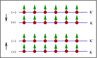
Figure 1: (Color online) Schematic diagram of four states of SU(4) Graphene in lowest $\Lambda$-level, where $\uparrow,\downarrow(+,-)$ represents physical spin (valley) states of the electron. Red-circled dot with arrow lines represents CS-CF quasiparticles, electron (circular dot) with attached magnetic flux (green arrow lines). Variation of the number of attached fluxes to each of the four species gives rise to different polarized states.

II Calculation proccedure

Following the Chern-Simon’s gauge field theory in SU(4) system, we have seen that the effective field depends on the quantum numbers (Spin and Valley) carried by the quassiparticles. The quasiparticles in CS theory experiences a mean effective magnetic field, $B^{*}_{\alpha}$

$$B^{*}_{\alpha}=B-\phi_{0}{\cal{K}}_{\alpha\beta}\;\rho_{\beta}$$ (1)

where $B$ is the applied actual magnetic filed, $\phi_{0}$ is the flux quanta. We label the valley-spin configurations $(+\uparrow),(+\downarrow),(-\uparrow),(-\downarrow)$ by $\alpha=1,2,3,4$ respectively as shown in fig 1. The indices $\alpha,\beta$ runs from $1$ to $4$, i.e. ${\cal K}_{\alpha\beta}$ is $4\times 4$ matrix

$$\cal{K}=\left(\begin{array}[]{llll}2k_{1}&m_{1}&n_{1}&n_{2}\\ m_{1}&2k_{2}&n_{3}&n_{4}\\ n_{1}&n_{2}&2k_{3}&m_{2}\\ n_{3}&n_{4}&m_{2}&2k_{4}\end{array}\right),$$ (2)

where $k$’s, $m$’s and $n$’s are positive integers including zero. In Ref. SM_SSM flux attachment scheme is represented schematically. As suggested by them we have also simplified the flux attachment that $k_{1}=k_{2},k_{3}=k_{4},n_{1}=n_{2}=n_{3}=n_{4}=n$. Considering mean-field approximation, the electron filling factor $\nu$ and the effective filling factor $\nu_{\alpha}$ of CS quasiparticles are related by,

$$\rho_{\alpha}/\nu_{\alpha}=\rho/\nu-{\cal K}_{\alpha\beta}\rho_{\beta}\;.$$ (3)

Selection of number of particles::

We have considered that $N$ number of corelated electrons resides on the spherical surface JainBook ; Fano's in presence of radial magnetic field created by a Dirac monopole at the center of the sphere with monopole strength $Q$ and there are $N_{1}$, $N_{2}$, $N_{3}$, $N_{4}$ number of electrons in species $1,2,3,4$ respectively.

$$N = N_{1}+N_{2}+N_{3}+N_{4}$$

$$S = \frac{N_{1}+N_{3}-N_{2}-N_{4}}{N_{1}+N_{2}+N_{3}+N_{4}}$$

$$V = \frac{N_{1}+N_{2}-N_{3}-N_{4}}{N_{1}+N_{2}+N_{3}+N_{4}}$$

$$M = \frac{N_{1}+N_{4}-N_{2}-N_{3}}{N_{1}+N_{2}+N_{3}+N_{4}}$$

We have chosen the values of $N_{1}$, $N_{2}$, $N_{3}$, $N_{4}$ such a way that it will give the value of $S$, $V$, $M$ in the following tables. The monopole strength corresponding to this field can be written as,

$$2q_{\alpha}=2Q-\sum_{\beta}(N_{\beta}-\delta_{\alpha\beta})\cal{K}_{\alpha\beta}$$ (4)

$$\sum_{\alpha}2q_{\alpha} = 8Q-\sum_{\alpha}\sum_{\beta}\left(N_{\alpha}-\delta_{\alpha\beta}\right)\cal{K}_{\alpha\beta}$$

$$\Rightarrow Q = \frac{1}{8}\left(\sum_{\alpha}2q_{\alpha}+\sum_{\alpha}{\cal K}_{\alpha\alpha}(N_{\alpha}-1)\right)$$

$$+ \frac{1}{8}\left(m_{1}N_{1}+m_{1}N_{2}+m_{2}N_{3}+m_{2}N_{4}+2nN\right)$$

2$Q\phi_{0}$ is the total flux through the spherical surface of radius $R$, if $B$ is the corresponding magnetic filed then

$$2Q\phi_{0}=4\pi R^{2}B\Rightarrow R^{2}=\frac{2Q}{4\pi}\frac{hc}{e}\frac{el^{2}}{\hbar c}=Q{l_{B}}^{2}$$

So the radius of the sphere is $R=\sqrt{Q}$ in unit of magnetic length $l_{B}$.

II.1 Wave function

Let us suppose that there are $\nu_{1}$ number of spin-up $(+)$ valley $\Lambda$-level, $\nu_{2}$ number of spin-down $(+)$ valley $\Lambda$-level, $\nu_{3}$ number of spin-up $(-)$ valley $\Lambda$-level, $\nu_{4}$ number of spin-down $(-)$ valley $\Lambda$-level. Following the route proposed by Mandal and co-workers the spin (S), the valley (V), and the mixed (M) polarization of these quasi-particles in a given FQH states is defined as,

$$S=(\rho_{1}+\rho_{3}-\rho_{2}-\rho_{4})/\rho,$$

$$V=(\rho_{1}+\rho_{2}-\rho_{3}-\rho_{4})/\rho,$$

$$M=(\rho_{1}+\rho_{4}-\rho_{2}-\rho_{3})/\rho,$$ (5)

So, the above equation (3) relates total filling factor $\nu$ in terms of those three polarization $S,V,M$ and the attached flux numbers k’s , m’s and n’s.

$$\gamma_{1}(2k_{1}+1/\nu_{1})+\gamma_{2}m_{1}+\eta_{1}2n=4/\nu$$

$$\gamma_{2}(2k_{1}+1/\nu_{2})+\gamma_{1}m_{1}+\eta_{1}2n=4/\nu$$

$$\gamma_{3}(2k_{3}+1/\nu_{3})+\gamma_{4}m_{2}+\eta_{2}2n=4/\nu$$

$$\gamma_{4}(2k_{3}+1/\nu_{4})+\gamma_{3}m_{2}+\eta_{2}2n=4/\nu$$ (6)

where, $\eta_{1(2)}=1-(+)V$, $\delta_{1(2)}=S-(+)M$, $\gamma_{1(2)}=\eta_{2}+(-)\delta_{2}$, and $\gamma_{3(4)}=\eta_{1}+(-)\delta_{1}$.

The five indices $k_{1}$, $k_{3}$, $m_{1}$, $m_{2}$, $n$ represent the interaction strength between different $\Lambda$-levels. From equation (6), it is very clear that the polarization index $S$, $V$, $M$; four species $\Lambda$-level filing fractions $\nu_{1},\nu_{2},\nu_{3},\nu_{4}$ and the interaction parameters $k_{1}$, $k_{3}$, $m_{1}$, $m_{2}$, $n$ altogether fixes the total filling fraction $\nu$ of the state. Here a particular state with fixed interaction parameters between the four species is symbolized as ($k_{1}k_{3}m_{1}m_{2}n$) at a certain filling fraction $\nu$.

II.1.1 Meaning of $(k_{1}k_{3}m_{1}m_{2}n)$

i. $2k_{1}$ number of flux attachment of CF in the ($+\uparrow$) and ($+\downarrow$) $\Lambda$-levels.
ii. $2k_{3}$ number of flux attachment of CF in the ($-\uparrow$) and ($-\downarrow$) $\Lambda$-levels.
iii. $m_{1}$ flux attachment in the ($+\uparrow$) level seen by the CFs in ($+\downarrow$) $\Lambda$-level and vice versa.
iv. $m_{2}$ flux attachment in the ($-\uparrow$) level seen by the CFs in ($-\downarrow$) $\Lambda$-level and vice versa.
v. $n$ flux attachment in the ($+\uparrow\&\downarrow$) level seen by the CFs in ($-\uparrow\&\downarrow$) $\Lambda$-levels and vice versa.

The variational wave function for the state is proposed by Mandal and coworker SM_SSM and is given by

$$\Psi_{\{\kappa_{\alpha\beta}\}} = {\cal P}_{L}\Phi_{\nu_{1}}(\Omega_{1}^{1},\cdots,\Omega_{N_{1}}^{1})\Phi_{\nu_{2}}(\Omega_{1}^{2},\cdots,\Omega_{N_{2}}^{2})$$

$$\times\Phi_{\nu_{3}}(\Omega_{1}^{3},\cdots,\Omega_{N_{3}}^{3})\Phi_{\nu_{4}}(\Omega_{1}^{4},\cdots,\Omega_{N_{4}}^{4})$$

$$\times J_{11}\;J_{22}\;J_{33}\;J_{44}\;J_{12}\;J_{34}\;J_{13}\;J_{14}\;J_{23}\;J_{24}$$

where, $\Phi_{\nu_{1}}$ is the Slater determinant of $\nu_{1}$ filled $\Lambda$ level CFs, $\Omega_{1},\cdots\Omega_{N_{\alpha}}$ are the positions of CFs on the spherical surface, upper index indicate the different species of CFs and the Jastrow factor is given by

$$J_{\alpha\beta} = \prod_{i,j}^{N_{\alpha},N_{\beta}}(u_{i}^{(\alpha)}v_{j}^{(\beta)}-u_{j}^{(\beta)}v_{i}^{(\alpha)})^{\kappa_{\alpha\beta}}\mbox{~{}~{}~{}~{} if $\alpha\;\neq\beta$ }$$

$$J_{\alpha\alpha} = \prod_{i<j}^{N_{\alpha}}(u_{i}^{(\alpha)}v_{j}^{(\alpha)}-u_{j}^{(\alpha)}v_{i}^{(\alpha)})^{\kappa_{\alpha\alpha}}$$

The prefix within bracket represent the CFs of different $\Lambda$ levels. Here we have used the spinor coordinates

$$u(\Omega)=cos(\theta/2)e^{-i\phi/2}\mbox{~{}~{}~{} and ~{}~{}~{}~{}}v(\Omega)=sin(\theta/2)e^{i\phi/2}$$

Some of the above wave functions are identical with the wave function proposed by Regnault and others using the plasma picture of the FQHE with internal SU(4) symmetry PRB77_2008 . The ground state energy ($E_{g}$) per particle corresponding to a particular state with flux attachment ($k_{1}k_{3}m_{1}m_{2}n$) can be calculated by the Monte Carlo method as

$$E_{g} = \frac{E+E_{bg}}{N}$$ (7)

$$= \left[\frac{<\Psi_{\{\kappa_{\alpha\beta}\}}|H|\Psi_{\{\kappa_{\alpha\beta}\}}>}{<\Psi_{\{\kappa_{\alpha\beta}\}}|\Psi_{\{\kappa_{\alpha\beta}\}}>}-\frac{N^{2}e^{2}}{2\epsilon R}\right]/N\;$$

Here, $H=\sum_{i<j}\frac{e^{2}}{r_{i,j}}$ is the Coulomb interaction, with $r_{i,j}$ as the inter-electronic distance and $E_{bg}=\frac{-N^{2}e^{2}}{2\epsilon R}$ term represents the background energy i.e. the interaction between the electrons and the background positive ions where $\epsilon$ is the dielectric constant of the background material. LL mixing parameter is independent of the applied magnetic field in the graphene system LLmixGraphene , so we do not need to include the LL mixing LLmix97 ; LLmix2009 in our calculation.

Table 1: Possible polarized states for filling fraction $\nu=1/2$ and their ground state energies with different parameters

$k_{1}$	$k_{3}$	$m_{1}$	$m_{2}$	$n$	$V$	$S$	$M$	$\nu_{1}$	$\nu_{2}$	$\nu_{3}$	$\nu_{4}$	$E_{g}(e^{2}/\epsilon l_{B})$
1	1	1	1	2								-0.4677
1	1	3	3	1	0	0	0	1	1	1	1	-0.46315
2	1	1	3	1								-0.45576
2	2	1	1	1								-0.44983
1	1	1	1	2				1	1	1	1	-0.46742
1	2	2	3	1								-0.46351
1	3	2	1	1	1/3	0	0	1	1	1	1	-0.46012
1	1	2	5	1								-0.45653
								1	1	0	0	-0.46321
					1	0	0	1	1	1	0	-0.46303
								1	1	0	1	-0.46298
1	1	1	1	2	-1	0	0	0	0	1	1	-0.46223
					1/4	0	0	1	1	1	1	-0.46759
					1/2	0	0	1	1	1	1	-0.46671
					2/3	0	0	1	1	1	1	-0.46567
1	1	1	1	3	1	0	0	1	1	0	0	-0.46321
					-1	0	0	0	0	1	1	-0.46223
1	2	1	1	1	1	0	0	1	1	0	0	-0.53459
2	1	1	1	1	-1	0	0	0	0	1	1	-0.53353
1	2	1	1	2	1	0	0	1	1	0	0	-0.46302
2	1	1	1	2	-1	0	0	0	0	1	1	-0.46186
					0	1	0	1	0	1	0	-0.51384
					0	-1	0	0	1	0	1	-0.51289
1	1	1	2	1	0	0	1	1	0	0	1	-0.51381
					0	0	-1	0	1	1	0	-0.51282
					0	1	0	1	0	1	0	-0.49495
					0	-1	0	0	1	0	1	-0.49391
1	1	2	2	1	0	0	1	1	0	0	1	-0.49514
					0	0	-1	0	1	1	0	-0.49398
					0	1	0	1	0	1	0	-0.49501
					0	-1	0	0	1	0	1	-0.49400
1	1	1	3	1	0	0	1	1	0	0	1	-0.49492
					0	0	-1	0	1	1	0	-0.49407

Figure 2: (Color online) Ground state energy per particle for different combinations of ($k_{1}k_{3}m_{1}m_{2}n$) with different values of polarization indices $V,S,M$ at filling fraction $\nu=1/2$.

Table 2: Lowest energy states with different polarization indices for $\nu=1/2$

$k_{1}$	$k_{3}$	$m_{1}$	$m_{2}$	$n$	$V$	$S$	$M$	$\nu_{1}$	$\nu_{2}$	$\nu_{3}$	$\nu_{4}$
1	1	1	1	2	0	0	0	1	1	1	1
					1/3	0	0	1	1	1	1
1	2	1	1	1	1	0	0	1	1	0	0
2	1	1	1	1	-1	0	0	0	0	1	1
					0	1	0	1	0	1	0
1	1	1	2	1	0	-1	0	0	1	0	1
					0	0	1	1	0	0	1
					0	0	-1	0	1	1	0

Table 3: Possible polarized states of filling fraction $\nu=1/4$ and their ground state energies with different parameters

$k_{1}$	$k_{3}$	$m_{1}$	$m_{2}$	$n$	$V$	$S$	$M$	$\nu_{1}$	$\nu_{2}$	$\nu_{3}$	$\nu_{4}$	$E_{g}(e^{2}/\epsilon l_{B})$
1	1	3	3	5				1	1	1	1	-0.21142
2	2	1	1	5				1	1	1	1	-0.17752
2	2	3	3	4	0	0	0	1	1	1	1	-0.35856
2	2	5	5	3				1	1	1	1	-0.35749
3	3	1	1	4				1	1	1	1	-0.33227
2	1	3	1	1	1	0	0	1	1	0	0	-0.45215
2	2	3	1	1	1	0	0	1	1	0	0	-0.45217
1	2	1	3	1	-1	0	0	0	0	1	1	-0.45178
2	2	1	3	1	-1	0	0	0	0	1	1	-0.45183
2	2	3	3	1	1	0	0	1	1	0	0	-0.45221
					-1	0	0	0	0	1	1	-0.45196
2	2	3	3	2	1	0	0	1	1	0	0	-0.41279
					-1	0	0	0	0	1	1	-0.41257
3	1	1	1	1	1	0	0	1	1	0	0	-0.42212
2	3	1	1	1	-1	0	0	0	0	1	1	-0.42164
					0	1	0	1	0	1	0	-0.41283
2	2	1	1	3	0	-1	0	0	1	0	1	-0.4125
					0	0	1	1	0	0	1	-0.41277
					0	0	-1	0	1	1	0	-0.41253
					0	1	0	1	0	1	0	-0.40453
2	2	1	2	3	0	-1	0	0	1	0	1	-0.40423
					0	0	1	1	0	0	1	-0.40439
					0	0	-1	0	1	1	0	-0.40407
					0	1	0	1	0	1	0	-0.40445
2	2	2	1	3	0	-1	0	0	1	0	1	-0.40423
					0	0	1	1	0	0	1	-0.40444
					0	0	-1	0	1	1	0	-0.40433
					0	1	0	1	0	1	0	-0.39658
2	2	2	2	3	0	-1	0	0	1	0	1	-0.39634
					0	0	1	1	0	0	1	-0.39654
					0	0	-1	0	1	1	0	-0.39646

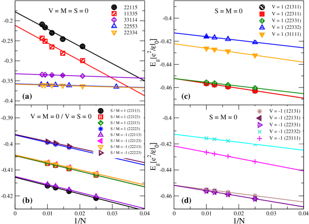
Figure 3: (Color online) Ground state energy per particle for different combinations of ($k_{1}k_{3}m_{1}m_{2}n$) with different values of polarization indices $V,S,M$ at filling fraction $\nu=1/4$.

Table 4: Lowest energy states of different polarization indices for $\nu=1/4$

$k_{1}$	$k_{3}$	$m_{1}$	$m_{2}$	$n$	$V$	$S$	$M$	$\nu_{1}$	$\nu_{2}$	$\nu_{3}$	$\nu_{4}$
2	2	3	3	4	0	0	0	1	1	1	1
2	2	5	5	3
2	1	3	1	1
2	2	3	1	1	1	0	0	1	1	0	0
2	2	3	3	1
1	2	1	3	1
2	2	1	3	1	-1	0	0	0	0	1	1
2	2	3	3	1
					0	1	0	1	0	1	0
2	2	1	1	3	0	-1	0	0	1	0	1
					0	0	1	1	0	0	1
					0	0	-1	0	1	1	0

III Results & Conclusion

We observed that the EDFQH states do not correspond to the Fermi sea of CFs. Zibrov et. al. Zibrov_Nat14 proposed that the EDFQH states are associated with a phase transition from a partial sublattice polarized PSP to a canted antiferromagnet phase CAF . With this idea, Sujit et. al. PRB98_2018 concluded that there is a phase transition from a state with $V\neq 0,S=0,M=0$ to one with $V=0$ and either $S$ or $M\neq 0$. They have noted also that the flux attachments for the state at $\nu=1/4$ are related to those found for $\nu=1/2$ by $j\rightarrow j+1$ for $j=k_{1},k_{3},m_{1},m_{2},n$ which agrees with our result too. In this article, we have accumulated all possible wave-functions for the recently observed EDFQH states at $\nu=1/2,1/4$ and calculated their ground state energies which help us to find out the befitted wave functions for those states. An understanding of the suitable ground state wave function for those two EDFQH states awaits future theoretical developments.

We have studied here the possible polarizations for the two EDFQH states ($\nu=1/2,1/4$). We have considered different combinations of flux attachment $(k_{1}k_{3}m_{1}m_{2}n)$ between the four species of electrons and calculated their ground state energies using the Coulomb potential for a finite number of particles. To get the thermodynamic limit, we have extrapolated the result in the $1/N\rightarrow 0$ region. The energy values for the filling fraction $\nu=1/2$ and $1/4$ are listed in TABLE 1 and TABLE 3. Energy has been expressed in natural unit $e^{2}/\epsilon l_{B}$ with respect to the spin and valley Zeeman energy. The error of the Monte-Carlo integration is less than the symbol size.
We have observed that different interaction strength between the four species can lead to different polarization. We can have the unpolarized state of $\nu=1/2$ for different combinations of flux attachment i.e. different interaction parameters; keeping the four $\Lambda$-level filling fractions unity ($\nu_{1}=\nu_{2}=\nu_{3}=\nu_{4}=1$). The ground state energies differ in each of the cases. We found that the state with interaction $(11112)$ has the lowest energy (see FIG. 2 (a)). So this is the most stable state for the unpolarized condition. Other states having interaction parameters $(11331)$, $(21131)$, $(22111)$ have higher energy compared to that. These states can be thought of as next stable states. By a slight change in the interaction parameters the system can suffer transition from one state to another. After that, we have considered different valley polarized states. We have observed that also for $V=1/3$ polarized state, with other two polarization index zero ($S$, $M=0$), the state with interaction $(11112)$ has the lowest energy (Fig. 2 (b)). Then we have checked the energies for different valley polarizations for the combination $(11112)$ keeping the spin and mixed polarization zero ($S=M=0$). Energies of those valley polarized states ($V=0,1/4,1/3,1/2,2/3,\pm 1$) are slightly differ from each other. So there is a high chance for the phase transition depending upon the Zeeman energies between the four $\Lambda$-levels. We have noted that $V=0$ state has the lowest energy and $V=\pm 1$ state has the highest energy and intermediate states lie in between. Besides, we have checked whether there is any other state having lower energy for $V=\pm 1$ polarization with other two polarization index ($S,M$) zero. We found that the states $(12111)$ and $(21111)$ have the lowest energy for the valley polarization $V=1$ and $V=-1$ respectively; with other two polarization index $S$, $M$ zero for both the two cases (see FIG. 2 (c)). Next, we calculated the same taking the polarization $S$ (or $M$) as $\pm 1$ and the other two polarization indices $V$, $M$ (or $V$, $S$) as zero, as suggested by Sujit et. al. PRB98_2018 . We observed that for the interaction $(11121)$ we get the lowest energy when the polarization $S$ (or, $M$) is $\pm 1$ and the energy values are almost equal (see FIG. 2 (d)). All the results for the filling fraction $\nu=1/2$ are shown in TABLE 2.

Similarly, we have checked all the above possibilities for the filling fraction $\nu=1/4$, the results are shown in Fig. 3 and in TABLE 3. For the unpolarized state ($V=S=M=0$), we have found that $(22334)$, $(22553)$ states have almost the same energy which is the lowest for this polarization (see FIG. 3 (a)). So the unpolarized state is doubly degenerate for $\nu=1/4$. We have found that for $V=1$ polarized state with other two polarization zero ($S$, $M=0$); $(21311)$, $(22311)$ and $(22331)$ states have the same energy value (see FIG. 3 (c)). That is those three states are degenerate metastable states; so the system can change any one of those. For the valley polarization $V=-1$ with $S$, $M=0$; there are also three degenerate metastable states, which are $(12131)$, $(22131)$, and $(22331)$ (see FIG. 3 (d)). We have found that $(22113)$ has the lowest energy when spin or mixed polarization $S$ (or, $M$) is $\pm 1$ and valley polarization is zero (see Fig. 3 (b)). We also noticed that for same interaction parameters ($22113$), change in Zeeman energies between four $\Lambda$-levels can lead to different polarization $S=\pm 1$, $M=\pm 1$ states, those states have same energies i.e. those are the degenerate states for the filling fraction $\nu=1/4$. The energy values for the different polarized states of filling fraction $\nu=1/4$ are enlisted in TABLE 4.

IV acknowledgement

Moumita thanks Dr. Debashis Das for the preliminary idea to start this work. She is thankful to the Department of Physics, IIEST Shibpur for providing her with the computing facility. Both of the two authors like to acknowledge Prof. Sudhansu Sekhar Mandal (IIT Kharagpur) for some fruitful discussions.

References

- (1) D. C. Tsui, H. L. Stormer, and A. C. Gossard, Phys. Rev. Lett. 48, 1559 (1982).
- (2) Laughlin, R. B., Phys. Rev. Lett. 50, 1395-1398 (1983).
- (3) J. K. Jain, Phys. Rev. Lett. 63, 199 (1989).
- (4) Composite Fermions, J. K. Jain (Cambridge University Press), http://www.cambridge.org/9780521862325.
- (5) I. V. Kukushkin, K. v. Klitzing and K. Eber, Phys. Rev. Lett. 82, 3665 (1999).
- (6) Ganpathy Murthy, Phys. Rev. Lett. 80, 350 (1999).
- (7) M. Indra, D. Das, D. Majumder; Phys. Lett. A 382 (2018), 2984–2988.
- (8) K. I. Bolotin, F. Ghahari, M. D. Shulman, H. L. Stormer, and P. Kim, Nature (London) 462, 196 (2009); X. Du, I. Skachko, F. Duerr, A. Luican, and E. Y. Andrei, Nature (London) 462, 192 (2009); D. A. Abanin, I. Skachko, X. Du, E. Y. Andrei, and L. S. Levitov, Phys. Rev. B 81, 115410 (2010); F. Ghahari, Y. Zhao, P. Cadden-Zimansky, K. Bolotin, and P. Kim, Phys. Rev. Lett. 106, 046801 (2011);
- (9) C. Pan, Y. Wu, B. Cheng, S. Che, T. Taniguchi, K. Watanabe, C. N. Lau, and M. Bock-rath, Nano Lett. 17 (6), pp 34163420 (2017); A. Kou, B. E. Feldman, A. J. Levin, B. I. Halperin, K. Watanabe, T. Taniguchi, and A. Yacoby Science 345, 55 (2014); Dong-Keun Ki, Vladimir I. Falko, Dmitry A. Abanin, and Alberto F. Morpurgo Nano Lett. 14, 2135 (2014).
- (10) A. H. Castro Neto, F. Guinea, N. M. R. Peres, K. S. Novoselov, and A. K. Geim, Rev. Mod. Phys. 81, 109 (2009).
- (11) K. Novoselov et. al., Nature 438, 197-200 (2005).
- (12) Zhang, Y., Tan, Y., Stormer, H. & Kim, P., Nature 438, 201-204 (2005).
- (13) Nomura, K. & MacDonald, A. H., Phys. Rev. Lett. 96, 256602 (2006).
- (14) Yang, K., Das Sarma, S. & MacDonald, A. H., Phys. Rev. B 74, 075423 (2006).
- (15) Dean, C. R., Young A. F., Cadden-Zimansky, P., Watanabe, K., Taniguchi, T., Kim, P., Hone, J., Shepard, K. L., Nature Physics 7, 693, (2011).
- (16) Shibata, N. & Nomura, K. Phys. Rev. B 77, 235426 (2008).
- (17) Csaba Toke, Jainendra K. Jain, Phys. Rev. B 75, 245440 (2007).
- (18) C Toke and J K Jain, J. Phys. Condens. Matter 24 (2012) 235601.
- (19) M. O. Goerbig and N. Regnault, Phys. Rev. B 75, 241405 R (2007).
- (20) Sanchita Modak, Sudhansu S. Mandal, and K. Sengupta, Phys. Rev. B 84, 165118 (2011).
- (21) A. Lopez, E. Fradkin, Phys. Rev. B 44 (1991) 5246.
- (22) A. A. Zibrov, E. M. Spanton, H. Zhou, C. Kometter, T. Taniguchi, K. Watanabe, and A. F. Young, Nat. Phys. 14, 930 (2018).
- (23) R. Willett, J. P. Eisenstein, H. L. Störmer, D. C. Tsui, A. C. Gossard, and J. H. English, Phys. Rev. Lett. 59, 1776 (1987).
- (24) J. Falson, D. Maryenko, B. Friess, D. Zhang, Y. Kozuka, A. Tsukazaki, J. H. Smet, and M. Kawasaki, Nat. Phys. 11, 347 (2015).
- (25) G. Moore and N. Read, Nucl. Phys. B 360, 362 (1991).
- (26) J. P. Eisenstein, G. S. Boebinger, L. N. Pfeiffer, K. W. West, and Song He, Phys. Rev. Lett. 68, 1383 (1992).
- (27) Y. W. Suen, L. W. Engel, M. B. Santos, M. Shayegan, and D. C. Tsui Phys. Rev. Lett. 68, 1379 (1992).
- (28) Y. W. Suen, H. C. Manoharan, X. Ying, M. B. Santos, and M. Shayegan, Phys. Rev. Lett. 72, 3405 (1994).
- (29) D. R. Luhman, W. Pan, D. C. Tsui, L. N. Pfeiffer, K. W. Baldwin, and K. W. West, Phys. Rev. Lett. 101, 266804 (2008).
- (30) J. Shabani, T. Gokmen, Y. T. Chiu, and M. Shayegan, Phys. Rev. Lett. 103, 256802 (2009).
- (31) C Toke and J K Jain, Phys. Rev. B 76, 081403(R) (2007).
- (32) K. Park, V. Melik-Alaverdian, N. E. Bonesteel, and J. K. Jain, Phys. Rev. B 58, R10167 (1998).
- (33) Song He, S. Das Sarma, and X. C. Xie, Phys. Rev. B 47, 4394 (1993).
- (34) R. de Gail, N. Regnault, and M. O. Goerbig, Phys. Rev. B 77, 165310 (2008).
- (35) B. I. Halperin, Helv. Phys. Acta 56, 75 (1983).
- (36) V. M. Apalkov and T. Chakraborty, Phys. Rev. Lett. 97, 126801 (2006).
- (37) Csaba Tőke, Paul E. Lammert, Vincent H. Crespi, and Jainendra K. Jain, Phys. Rev. B 74, 235417 (2006).
- (38) D. V. Khveshchenko, Phys. Rev. B 75, 153405 (2007).
- (39) Ajit C. Balram, Csaba Toke, A. Wojs, and J. K. Jain, Phys. Rev. B 92, 075410 (2015).
- (40) T. Gokmen, Medini Padmanabhan, and M. Shayegan, Phys. Rev. B 81, 235305 (2010).
- (41) Z. Papic, M. O. Goerbig, and N. Regnault Phys. Rev. Lett. 105 176802 (2010).
- (42) Sujit Narayanan, Bitan Roy and Malcolm P. Kennett, Phys. Rev. B 98, 235411 (2018).
- (43) G. Fano, F. Ortolani and E. Colombo, Phys. Rev. B 34, 2670 (1986).
- (44) Michael R. Peterson and Chetan Nayak, Phys. Rev. Lett. 113, 086401 (2014).
- (45) V. Melik-Alaverdian and N. E. Bonesteel, Phys. Rev. Lett. 79, 5286 (1997).
- (46) Waheb Bishara and Chetan Nayak, Phys. Rev. B 80, 121302(R) (2009).
- (47) Kentaro Nomura, Shinsei Ryu, and Dung-Hai Lee, Phys. Rev. Lett. 103, 216801, (2009).
- (48) Igor F. Herbut, Phys. Rev. B 75, 165411, (2007).