A two-stage approach for a mixed-integer economic dispatch game in integrated electrical and gas distribution systems

Abstract

We formulate for the first time the economic dispatch problem in an integrated electrical and gas distribution system as a game equilibrium problem between distributed prosumers. Specifically, by approximating the non-linear gas-flow equations either with a mixed-integer second order cone or a piece-wise affine model and by assuming that electricity and gas prices depend linearly on the total consumption we obtain a potential mixed-integer game. To compute an approximate generalized Nash equilibrium, we propose an iterative two-stage method that exploits a problem convexification and the gas flow models. We quantify the quality of the computed solution and perform a numerical study to evaluate the performance of our method.

economic dispatch, integrated electrical and gas systems, generalized mixed-integer games

1 Introduction

One of the key features of future energy systems is the decentralization of power generation [1, 2], where small-scale distributed generators (DGs) will have a major contribution in meeting energy demands. Furthermore, the intermittency of renewable power generation might necessitate the co-existence of non-renewable yet controllable DGs to provide enough supply and offer flexibility [1, Sec. 3]. In this context, gas-fired generators, such as combined heat and power (CHP) [3, 4], can play a prominent role due to its efficiency and infrastructure availability. Consequently, electrical and gas systems are expected to be more intertwined in the future and in fact, this integration has received research attention in the control systems community [5, 6, 7, 8, 9].

Several works, e.g. [9, 10, 11, 12, 13, 14, 15, 16, 17, 18, 19], particularly study the tertiary control problem for an integrated electrical and gas system (IEGS), i.e., the problem of computing optimal operating points for the generators. In these papers, the economic dispatch problem is posed as an optimization program where the main objective is to minimize the operational cost of the whole network, which includes electrical and gas production costs, subject to physical dynamics and operational constraints. Differently from [10, 11, 12, 13, 14, 15, 16, 17, 18, 19, 9], where a common objective is considered, when DGs are owned by different independent entities (prosumers), the operations of these DGs depend on several individual objectives. In the latter case, to compute optimal operating points of its DG, each prosumer must solve its own economic dispatch problem. However, these prosumers are coupled with each other as they share a common power (and possibly gas) distribution network. Their objective functions can also depend on the decisions of other prosumers, such as via an energy price function [20, 21]. Therefore, the economic dispatch problems of prosumers in an IEGS is naturally a generalized game [22]. When each prosumer aims at finding a decision that optimizes its objective given the decisions of others, we obtain a generalized Nash equilibrium (GNE) problem, i.e., the problem of finding a GNE, a point where each player has no incentive to unilaterally deviate.

For a jointly convex game, i.e., when the cost function of each player is convex with respect to the player’s strategy and the global feasible set is convex, efficient algorithmic solutions to solve a GNE problem are available in the literature, e.g., [23, 24, 25, 26]. However, the economic dispatch problem in an IEGS system is typically formulated as a mixed-integer optimization program due to the approximation methods commonly used for non-linear gas-flow equations. For instance, [14, 16, 15, 17] consider mixed-integer second-order cone (MISOC) gas-flow models whereas [10, 11, 12, 13] use mixed-integer linear ones. On account of mixed-integer nature of the problem, the GNE seeking methods in [23, 24, 25, 26] are not applicable and in fact, there are only a few works that propose GNE-seeking methods for mixed-integer generalized games, e.g., [27, 28, 29, 30].

In this paper, we formulate an economic dispatch problem in an integrated electrical and gas distribution system (IEGDS) as a mixed-integer generalized game (Section 2). Specifically, we consider prosumers, i.e., the entities that own active components, namely DGs and storage units, as the players of the game. Aside from consuming electricity and gas, each prosumer can produce and/or store electrical power as well as buy power and gas from the main grid, where the prices depend linearly on the aggregate consumption. Furthermore, our formulation can incorporate a piece-wise affine (PWA) gas flow approximation, yielding a set of mixed-integer linear constraints, or a classic MISOC relaxation. The game-theoretic formulation is the main conceptual novelty of this paper compared to the existing literature in IEGDSs. To our knowledge, there are only a few works, e.g. [31, 32], that discuss the dispatch of IEGDS systems as a (jointly convex) generalized game, but under a substantially different setup, i.e., a two-player game between the electrical and gas network operators, subject to a perfect-pricing assumption.

Then, we propose a novel two-stage approach to compute a solution of the economic dispatch game, namely a(n) (approximate) mixed-integer GNE (MI-GNE) (Section 3). In the first stage, we relax the problem into a jointly convex game and compute a GNE of the convexified game. Next, in the second stage we recover a mixed-integer solution, which has minimum gas-flow violation, by exploiting the gas flow models and by solving a linear program. Furthermore, we can refine the computed solution by iterating these steps. In these iterations, we introduce an auxiliary penalty function on the gas-flows to the convexified game and adjust its penalty weight. Consequently, we can provide a condition when our iterative algorithm obtains an (approximate) MI-GNE and measure the solution quality (Theorem 1). Differently from other existing MI-GNE seeking methods [27, 28, 29, 30], our method allows for a parallel implementation and does not solve a mixed-integer optimization. We also remark that existing distributed parallel mixed-integer optimization algorithms, e.g. [33, 34], only deal with linear objective functions; therefore, they are unsuitable for our case. In Section 4, we show the performance of our algorithm via numerical simulations of a benchmark 33-bus-20-node distribution network. We note that, in the preliminary work [35], we only consider the PWA gas flow model and implement the two stage approach without the refining iterations to compute an approximate solution to the economic dispatch problem of multi-area IEGSs [13, 16, 19], which is an optimization problem with a common and separable cost function, instead of a noncooperative game.

Notation

We denote by $\mathbb{R}$ and $\mathbb{N}$ the set of real numbers and that of natural numbers, respectively. We denote by $\bm{0}$ ($\bm{1}$) a matrix/vector with all elements equal to $0$ ($1$). The Kronecker product between the matrices $A$ and $B$ is denoted by $A\otimes B$. For a matrix $A\in\mathbb{R}^{n\times m}$, its transpose is $A^{\top}$. For symmetric $A\in\mathbb{R}^{n\times n}$, $A\succ 0$ ($\succcurlyeq 0$) stands for positive definite (semidefinite) matrix. The operator $\operatorname{col}(\cdot)$ stacks its arguments into a column vector whereas $\operatorname{diag}(\cdot)$ ($\operatorname{blkdiag}(\cdot)$) creates a (block) diagonal matrix with its arguments as the (block) diagonal elements. The sign operator is denoted by $\operatorname{sgn}(\cdot)$, i.e.,

$$\operatorname{sgn}(a)=\begin{cases}1\quad&\text{if }a>0,\\ 0\quad&\text{if }a=0,\\ -1\quad&\text{if }a<0.\end{cases}$$

2 Economic dispatch game

In this section, we formulate the economic dispatch game of a set of $N$ prosumers (agents), denoted by $\mathcal{I}:=\{1,2,\dots,N\}$, in an IEGDS. Each prosumer seeks an economically efficient decision (optimal references/set points) to meet its electrical and gas demands over a certain time horizon, denoted by $H$; let us denote the set of time indices by $\mathcal{H}:=\{1,\dots,H\}$. First, we provide the model of the system, which consists of two parts, the electrical and gas networks.

2.1 Electrical network

To meet the electrical demands, denoted by $d_{i}^{\mathrm{e}}\in\mathbb{R}^{H}_{\geq 0}$ for all $i\in\mathcal{I}$, the prosumers may have a dispatchable DG, which can be either gas-fueled or non-gas-fueled. We denote the set of agents that have a gas-fueled unit by $\mathcal{I}^{\mathrm{gu}}\subset\mathcal{I}$ whereas those that have a non-gas-fueled unit by $\mathcal{I}^{\mathrm{ngu}}\subset\mathcal{I}$. We note that $\mathcal{I}^{\mathrm{dg}}:=\mathcal{I}^{\mathrm{gu}}\cup\mathcal{I}^{\mathrm{ngu}}\subseteq\mathcal{I}$. For each $i\in\mathcal{I}^{\mathrm{dg}}$, let us denote the power produced by its generation unit by $p_{i}^{\mathrm{dg}}\in\mathbb{R}_{\geq 0}^{H}$, constrained by

$$\mathbf{1}_{H}\,\underline{p}_{i}^{\mathrm{dg}}\leq p_{i}^{\mathrm{dg}} \leq\mathbf{1}_{H}\,\overline{p}_{i}^{\mathrm{dg}},$$ (1)

where $\underline{p}_{i}^{\mathrm{dg}}<\overline{p}_{i}^{\mathrm{dg}}$ denote the minimum and maximum power production. Specifically for the prosumers with non-gas-fueled DGs, we consider a quadratic cost of producing power, i.e.,

$$f_{i}^{\mathrm{ngu}}(p_{i}^{\mathrm{dg}})=\begin{cases}q_{i}^{\mathrm{ngu}}\|p_{i}^{\mathrm{dg}}\|^{2}+l_{i}^{\mathrm{ngu}}\mathbf{1}^{\top}p_{i}^{\mathrm{dg}},\ &\text{if }i\in\mathcal{I}^{\mathrm{ngu}},\\ 0,\quad&\text{otherwise,}\end{cases}$$ (2)

where $q_{i}^{\mathrm{ngu}}>0$ and $l_{i}^{\mathrm{ngu}}$ are constants. On the other hand, for the prosumers with gas-fueled DGs, we assume a linear relationship between the consumed gas, $d_{i}^{\mathrm{gu}}$, and the produced power, as in [17, Eq. (24)], i.e.,

$$d_{i}^{\mathrm{gu}}=\begin{cases}\eta_{i}^{\mathrm{gu}}p_{i}^{\mathrm{dg}},\quad&\text{if }i\in\mathcal{I}^{\mathrm{gu}},\\ 0,\quad&\text{otherwise},\end{cases}$$ (3)

where $\eta_{i}^{\mathrm{gu}}>0$ denotes the conversion factor.

Each prosumer might also own a controllable storage unit, whose cost function, which corresponds to reducing its degradation, is denoted by $f_{i}^{\mathrm{st}}:\mathbb{R}^{2H}\to\mathbb{R}$:

$$f_{i}^{\mathrm{st}}(p_{i}^{\mathrm{ch}},p_{i}^{\mathrm{dh}})=(p_{i}^{\mathrm{ch}})^{\top}Q_{i}^{\mathrm{st}}p_{i}^{\mathrm{ch}}+(p_{i}^{\mathrm{dh}})^{\top}Q_{i}^{\mathrm{st}}p_{i}^{\mathrm{dh}},$$ (4)

where $Q_{i}^{\mathrm{st}}\succcurlyeq 0$. The variables $p_{i}^{\mathrm{ch}}=\operatorname{col}((p_{i,h}^{\mathrm{ch}})_{h\in\mathcal{H}})$ and $p_{i}^{\mathrm{dh}}=\operatorname{col}((p_{i,h}^{\mathrm{dh}})_{h\in\mathcal{H}})$ denote the charging and discharging powers, which are constrained by the battery dynamics and operational limits [4, Eqs. (1)–(3)]:

$$\left.\begin{array}[]{c}x_{i,h+1}=\eta_{i}^{\mathrm{st}}x_{i,h}+\frac{T_{\mathrm{s}}}{e^{\mathrm{cap}}_{i}}(\eta_{i}^{\mathrm{ch}}p_{i,h}^{\mathrm{ch}}-(\frac{1}{\eta_{i}^{\mathrm{dh}}})p_{i,h}^{\mathrm{dh}}),\\[1.99997pt] \underline{x}_{i}\leq x_{i,h+1}\leq\overline{x}_{i},\\[1.99997pt] \end{array}\right\} \begin{matrix}\forall i\in\mathcal{I}^{\mathrm{st}},\\ \forall h\in\mathcal{H},\end{matrix}$$ (5)

$${p}_{i}^{\mathrm{ch}}\in[0,\overline{{p}}_{i}^{\mathrm{ch}}],\ \ {p}_{i}^{\mathrm{dh}}\in[0,\overline{{p}}_{i}^{\mathrm{dh}}], \forall i\in\mathcal{I}^{\mathrm{st}},$$

$$p_{i}^{\mathrm{ch}}=0,\ \ p_{i}^{\mathrm{dh}}=0, \forall i\in{\mathcal{I}\backslash\mathcal{I}^{\mathrm{st}},}$$

where $x_{i,h}$ denotes the state of charge (SoC) of the storage unit at time $h\in\mathcal{H}$, $\eta_{i}^{\mathrm{st}},\eta_{i}^{\mathrm{ch}},\eta_{i}^{\mathrm{dh}}\in(0,1]$ denote the leakage coefficient of the storage, charging, and discharging efficiencies, respectively, while $T_{\mathrm{s}}$ and $e^{\mathrm{cap}}_{i}$ denote the sampling time and the maximum capacity of the storage, respectively. Moreover, $\underline{x}_{i},\overline{x}_{i}\in[0,1]$ denote the minimum and the maximum SoC of the storage unit of prosumer $i$, respectively, whereas $\overline{p}^{\mathrm{ch}}_{i}\geq 0$ and $\overline{p}^{\mathrm{dh}}_{i}\geq 0$ denote the maximum charging and discharging power of the storage unit. Finally, we denote by $\mathcal{I}^{\mathrm{st}}\subseteq\mathcal{I}$ the set of prosumers that own a storage unit.

These prosumers may also buy electrical power from the main grid, and we denote this decision by $p_{i}^{\mathrm{eg}}:=\operatorname{col}((p_{i,h}^{\mathrm{eg}})_{h\in\mathcal{H}})\in\mathbb{R}^{H}_{\geq 0}$, where $p_{i,h}^{\mathrm{eg}}$ denotes the decision at time step $h$. We consider a typical assumption in demand-side management, namely that the electricity price depends on the total consumption of the network of prosumers, which is usually defined as a quadratic function [20, Eq. (12)], i.e.,

$$c_{h}^{\mathrm{e}}(\sigma^{\mathrm{e}}_{h})=q_{h}^{\mathrm{e}}(\sigma^{\mathrm{e}}_{h})^{2}+l_{h}^{\mathrm{e}}\sigma^{\mathrm{e}}_{h},$$

where $\sigma^{\mathrm{e}}_{h}$ denotes the aggregate load on the main electrical grid, i.e., $\sigma^{\mathrm{e}}_{h}=\sum_{i\in\mathcal{I}}p_{i,h}^{\mathrm{eg}},$ and $q_{h}^{\mathrm{e}},l_{h}^{\mathrm{e}}\geq 0$ are constants. Therefore, by denoting $\sigma^{\mathrm{e}}=\operatorname{col}(\{\sigma^{\mathrm{e}}_{h}\})$, the objective function of agent $i$ associated to the trading with the main grid, denoted by $f_{i}^{\mathrm{eg}}$, is defined as

$$\textstyle f_{i}^{\mathrm{e}}\left(p_{i}^{\mathrm{eg}},\sigma^{\mathrm{e}}\right) =\sum_{h\in\mathcal{H}}c_{h}^{\mathrm{e}}(\sigma^{\mathrm{e}}_{h})\frac{p_{i,h}^{\mathrm{eg}}}{\sum_{j\in\mathcal{I}}p_{j,h}^{\mathrm{eg}}}$$ (6)

$$=\sum_{h\in\mathcal{H}}q_{h}^{\mathrm{e}}\cdot\Big{(}\sum_{j\in\mathcal{I}}p_{j,h}^{\mathrm{eg}}\Big{)}\cdot p_{i,h}^{\mathrm{eg}}+l_{h}^{\mathrm{e}}.$$

Moreover, we impose that the aggregate power traded with the main grid is bounded as follows:

$$\mathbf{1}_{H}\,\underline{\sigma}^{\mathrm{e}}\leq\sum_{i\in\mathcal{I}}p_{i}^{\mathrm{eg}}\leq\mathbf{1}_{H}\,\overline{\sigma}^{\mathrm{e}},$$ (7)

where $\overline{\sigma}^{\mathrm{e}}>\underline{\sigma}^{\mathrm{e}}\geq 0$ denote the upper and lower bounds. Note that the lower bound might be required to be positive in order to ensure a continuous operation of the main generators that supply the main grid.

Next, we describe the physical constraints of the electrical network. For ease of exposition, we assume that each agent is associated with a bus (node) in an electrical distribution network, which can be represented by an undirected graph $\mathcal{G}^{\mathrm{e}}:=(\mathcal{I},\mathcal{E}^{\mathrm{e}})$, where $\mathcal{E}^{\mathrm{e}}$ denotes the set of power lines. Therefore, we denote by $\mathcal{N}_{i}^{\mathrm{e}}$ the set of neighbor nodes of node $i$, i.e., $\mathcal{N}_{i}^{\mathrm{e}}:=\{j\mid(i,j)\in\mathcal{E}^{\mathrm{e}}\}$. Let us then denote by $\theta_{i}\in\mathbb{R}^{H}$ and $v_{i}\in\mathbb{R}^{H}$ the voltage angle and magnitude of bus $i\in\mathcal{I}$ while by $p_{(i,j)}^{\ell},q_{(i,j)}^{\ell}\in\mathbb{R}^{H}$ the active and reactive powers of line $(i,j)\in\mathcal{E}^{\mathrm{e}}$.

The voltage phase angle ($\theta_{i}$) and magnitude ($v_{i}$) for each node $i\in\mathcal{I}$ are bounded by

$$\underline{\theta}_{i}\mathbf{1}\leq\theta_{i} \leq\overline{\theta}_{i}\mathbf{1},$$ (8a)

$$\underline{v}_{i}\mathbf{1}\leq v_{i} \leq\overline{v}_{i}\mathbf{1},$$ (8b)

where $\underline{\theta}_{i}\leq\overline{\theta}_{i}$ denote the minimum and maximum phase angles and $\underline{v}_{i}\leq\overline{v}_{i}$ denote the minimum and maximum voltages. Without loss of generality, we suppose the reference is bus $1$ and assume $\underline{\theta}_{1}=\overline{\theta}_{1}=0$.

The power balance equation, which ensures equal production and consumption, at each bus can be written as:

$$d_{i}^{\mathrm{e}} =p_{i}^{\mathrm{dg}}+p_{i}^{\mathrm{eg}}+p_{i}^{\mathrm{dh}}-p_{i}^{\mathrm{ch}}, \forall i\in\mathcal{I},$$ (9a)

$$p_{i}^{\mathrm{eg}} =p_{i}^{\mathrm{et}}-\sum_{j\in\mathcal{N}_{i}}p_{(i,j)}^{\ell}, \forall i\in\mathcal{I},$$ (9b)

where $p_{i}^{\mathrm{et}}$ denotes the injected power from the electrical transmission grid if node $i$ is connected to it and $p_{(i,j)}^{\ell}$, for each $j\in\mathcal{N}_{i}$, denote the real power line between node $i$ and its neighbor $j$. Furthermore, for simplicity, we use a linear approximation of the real power-flow equations [36, Eq. (2)],

$$p_{(i,j)}^{\ell}=B_{(i,j)}\left({\theta_{i}-\theta_{j}}\right)-G_{(i,j)}\left(v_{i}-v_{j}\right),\,\,\forall j\in\mathcal{N}_{i}^{\mathrm{e}},$$ (10)

for each $i\in\mathcal{I}$, where $B_{(i,j)}$ and $G_{(i,j)}$ denote the absolute values of the susceptance and conductance of line $(i,j)$, respectively. Finally, let us now collect all the decision variables associated with the electrical network by $x_{i}:=\operatorname{col}(p_{i}^{\mathrm{dg}},p_{i}^{\mathrm{ch}},p_{i}^{\mathrm{dh}},p_{i}^{\mathrm{eg}},d_{i}^{\mathrm{gu}},\theta_{i},v_{i},p_{i}^{\mathrm{et}},\{p_{(i,j)}^{\mathrm{\ell}}\}_{j\in\mathcal{N}_{i}^{{\mathrm{e}}}})\in\mathbb{R}^{n_{x_{i}}}$, with $n_{x_{i}}=H(8+\mathcal{N}_{i}^{\mathrm{e}})$, for each $i\in\mathcal{N}$.

2.2 Gas network

Beside consuming $d_{i}^{\mathrm{gu}}\in\mathbb{R}_{\geq 0}^{H}$ for its gas-fired generator, we suppose that prosumer $i$ has an undispatchable gas demand, denoted by $d_{i}^{\mathrm{g}}\in\mathbb{R}_{\geq 0}^{H}$. The total gas demand of each prosumer is satisfied by buying gas from a source, which can either be a gas transmission network or a gas well. These prosumers are connected in a gas distribution network, represented by an undirected graph denoted by $\mathcal{G}^{\mathrm{g}}=(\mathcal{I},\mathcal{E}^{\mathrm{g}})$, where we assume that each agent is a different node in $\mathcal{G}^{\mathrm{g}}$ and denote by $\mathcal{E}^{\mathrm{g}}$ the set of pipelines (links), where both $(i,j),(j,i)\in\mathcal{E}^{\mathrm{g}}$ represent the pipeline between nodes $i$ and $j$. If node $j$ is connected to node $i$, then node $j$ belongs to the set of neighbors of node $i$ in the gas network, denoted by $\mathcal{N}_{i}^{\mathrm{g}}:=\{j\in\mathcal{N}^{\mathrm{g}}\mid(i,j)\in\mathcal{E}^{\mathrm{g}}\}$. Therefore, the gas-balance equation of node $i\in{\mathcal{I}}$ can be written as:

$$g_{i}^{\mathrm{s}}-d_{i}^{\mathrm{g}}-d_{i}^{\mathrm{gu}} =\sum_{j\in\mathcal{N}_{i}^{\mathrm{g}}}\phi_{(i,j)},$$ (11)

where $g_{i}^{\mathrm{s}}\in\mathbb{R}_{\geq 0}^{H}$ denotes the imported gas from a source, if agent $i$ is connected to it. We denote the set of nodes connected to the gas source by $\mathcal{I}^{\mathrm{gs}}$. Moreover, $\phi_{(i,j)}:=\operatorname{col}((\phi_{(i,j),h})_{h\in\mathcal{H}})\in\mathbb{R}^{H}$ denotes the flow between nodes $i$ and $j$ from the perspective of agent $i$, i.e., $\phi_{(i,j),h}>0$ implies the gas flows from node $i$ to node $j$. We formulate the cost of buying gas similarly to that of importing power from the main grid as these prosumers must pay the gas with a common price that may vary. Specifically, with the per-unit cost that depends on the total gas consumption, we have the following cost functions ($\forall i\in\mathcal{I}$):

$$f_{i}^{\mathrm{g}}(d_{i}^{\mathrm{gu}},\sigma^{\mathrm{g}})=\sum_{h\in\mathcal{H}}q_{h}^{\mathrm{g}}\cdot\sigma_{h}^{\mathrm{g}}\cdot(d_{i,h}^{\mathrm{gu}}+d_{i,h}^{\mathrm{g}})+l_{h}^{\mathrm{g}},$$ (12)

where $q_{h}^{\mathrm{g}}>0$ and $l_{h}^{\mathrm{g}}\in\mathbb{R}$ are the cost parameters whereas $\sigma^{\mathrm{g}}=\operatorname{col}(\{\sigma_{h}^{\mathrm{g}}\}_{h\in\mathcal{H}})$ with $\sigma_{h}^{\mathrm{g}}=\sum_{i\in\mathcal{I}}(d_{i,h}^{\mathrm{gu}}+d_{i,h}^{\mathrm{g}}),$ which denotes the aggregated gas demand. In addition, the following constraints on the gas network are typically considered:

• Weymouth gas-flow equation for two neighboring nodes:

  $$\phi_{(i,j),h}=\operatorname{sgn}(\psi_{i,h}-\psi_{j,h})c_{(i,j)}^{\mathrm{f}}\sqrt{|\psi_{i,h}-\psi_{j,h}|},$$ (13)

  for all $h\in\mathcal{H}$, $j\in\mathcal{N}_{i}^{\mathrm{g}}$, and $i\in\mathcal{I}^{\mathrm{g}}$, where $\psi_{i,h}\in\mathbb{R}_{\geq 0}$ is the squared pressure at node $i$, and $c_{(i,j)}^{\mathrm{f}}>0$ is some constant. We define $\psi_{i}=\operatorname{col}((\psi_{i,h})_{h\in\mathcal{H}})$. By assuming a sufficiently large sampling time, we consider static gas flow equations as in, e.g. [14, 15, 16, 17], instead of dynamic ones such as [9, 8].

• Bounds on the gas flow $\phi_{(i,j)}$ and the pressure $\psi_{i}$:

  $$-\mathbf{1}_{H}\,\overline{\phi}_{(i,j)}\leq\phi_{(i,j)}\leq\mathbf{1}_{H}\,\overline{\phi}_{(i,j)},\ \ \forall j\in\mathcal{N}_{i}^{\mathrm{g}},i\in\mathcal{I},$$ (14)

  $$\mathbf{1}_{H}\,\underline{\psi}_{i}\leq\psi_{i}\leq\mathbf{1}_{H}\,\overline{\psi}_{i},\ \ \forall i\in\mathcal{I},$$ (15)

  $$g_{i}^{\mathrm{s}}=0,\ \ \forall i\in{\mathcal{I}\backslash\mathcal{I}^{\mathrm{gs}},}$$ (16)

  where $\overline{\phi}_{(i,j)}$ denotes the maximum flow of the link $(i,j)\in\mathcal{E}^{\mathrm{g}}$ whereas $\underline{\psi}_{i}$ and $\overline{\psi}_{i}$ denote the minimum and maximum (squared) gas pressure of node $i$, respectively. The constraint in (16) ensures that gas only flows through the nodes that are connected to a gas source.

• Bounds on the total gas consumption of the network $\mathcal{G}^{\mathrm{g}}$:

  $$\mathbf{1}_{H}\underline{\sigma}^{\mathrm{g}}\leq\sum_{i\in\mathcal{N}^{\mathrm{g}}}(d_{i}^{\mathrm{g}}+d_{i}^{\mathrm{dg}})\leq\mathbf{1}_{H}\overline{\sigma}^{\mathrm{g}},$$ (17)

  where $\underline{\sigma}^{\mathrm{g}}$ and $\overline{\sigma}^{\mathrm{g}}$ denote the minimum and maximum total gas consumption of the distribution network $\mathcal{G}^{\mathrm{g}}$, respectively.

2.3 Approximation models of gas-flow equations

The gas-flow equations in (13) are nonlinear and in fact introduce non-convexity to the decision problem. In this work, we consider two models that are commonly used in the literature, namely the MISOC relaxation and the PWA approximation. In the former, the gas flow equation is reformulated and relaxed into inequality constraints, whereas in the latter it is approximated by a PWA function. Both models require the introduction of auxiliary continuous and binary variables, collected in the vectors $y_{i}$ and $z_{i}$, for each $i\in\mathcal{I}$, respectively. For ease of presentation, we represent the two models as a set of equality and inequality constraints:

$$h_{i}^{\mathrm{cpl}}(y_{i},\{y_{j}\}_{j\in\mathcal{N}_{i}^{\mathrm{g}}})=0,\ \ \forall i\in\mathcal{I},$$ (18)

$$h_{i}^{\mathrm{loc}}(y_{i},z_{i})=0,\ \ \forall i\in\mathcal{I},$$ (19)

$$g_{i}^{\mathrm{cpl}}(y_{i},z_{i},\{y_{j}\}_{j\in\mathcal{N}_{i}^{\mathrm{g}}})\leq 0,\ \ \forall i\in\mathcal{I},$$ (20)

$$g_{i}^{\mathrm{loc}}(y_{i},z_{i})\leq 0,\ \ \forall i\in\mathcal{I},$$ (21)

where (18) and (20) are coupling constraints since $h_{i}^{\mathrm{cpl}}$ and $g_{i}^{\mathrm{cpl}}$ depend on the decision variables of the neighbors in $\mathcal{N}_{i}^{\mathrm{g}}$ while (19) and (21) are local constraints.

We now briefly explain the MISOC and PWA models and introduce their auxiliary variables.

MISOC model

We can obtain the MISOC model by relaxing the gas-flow constraints in (13) into inequality constraints, introducing a binary variable to indicate each flow direction, and using the McCormick envelope to substitute the product of two decision variables with an auxiliary variable, denoted by $\nu_{(i,j)}\in\mathbb{R}^{H}$, for each $j\in\mathcal{N}_{i}^{\mathrm{g}}$ and $i\in\mathcal{I}$. We provide the detailed derivation in Appendix 6.1. For this model, $y_{i}:=\operatorname{col}(\psi_{i},g_{i}^{\mathrm{s}},\{\phi_{(i,j)},\nu_{(i,j)}\}_{j\in\mathcal{N}_{i}^{\mathrm{g}}})\in\mathbb{R}^{n_{y_{i}}}$, with $n_{y_{i}}=H(2+2|\mathcal{N}_{i}^{\mathrm{g}}|)$, concatenates the physical variables of the gas network, i.e., $\psi_{i}$, $g_{i}^{\mathrm{s}}$, and $\phi_{(i,j)}$, for all $j\in\mathcal{N}_{i}^{\mathrm{g}}$, with the auxiliary variables $\nu_{(i,j)}$, whereas $z_{i}:=\operatorname{col}(\{\delta_{(i,j)}\}_{j\in\mathcal{N}_{i}^{\mathrm{g}}})\in\{0,1\}^{n_{z_{i}}}$, with $n_{z_{i}}=H|\mathcal{N}_{i}^{\mathrm{g}}|$, collects the binary decision vectors that indicate the flow directions. The coupling constraints for this model are affine. Furthermore, this model includes a set of convex second order cone (SOC) local constraints and does not have any local equality constraints. We note that if the gas flow directions (binary variables) are known, then the model becomes convex. Furthermore, when the SOC local constraints of the MISOC model are tight, the original gas flow constraints in (13) are satisfied. However, we cannot guarantee the tightness of the SOC constraints in general, although one can use a penalty-based method [16] or sequential cone programming method [31, 16] to induce tightness.

PWA model

We obtain the PWA model by approximating the mapping $\phi_{(i,j),h}\mapsto(1/{c_{(i,j)}^{\mathrm{f}}})^{2}{\phi_{(i,j),h}^{2}}$, for each $(i,j)\in\mathcal{E}^{\mathrm{g}}$, with $r$ pieces of affine functions. Then we can use this approximation in (13). Furthermore, by utilizing the mixed-logical constraint reformulation [37], we obtain an approximated model of the gas-flow constraints as a set of mixed-integer linear constraints, as detailed in Appendix 6.2. In this model, for each $i\in\mathcal{I}$, we introduce some auxiliary continuous variables $\nu_{(i,j)}^{\psi}\in\mathbb{R}^{H}$, for all $j\in\mathcal{N}_{i}^{\mathrm{g}}$, and $\nu_{(i,j)}^{m}\in\mathbb{R}^{H}$, for $m=1,\dots,r$ and all $j\in\mathcal{N}_{i}^{\mathrm{g}}$, and thus, define $y_{i}:=\operatorname{col}(\psi_{i},g_{i}^{\mathrm{s}},\{\phi_{(i,j)},\nu_{(i,j)}^{\psi},\{\nu_{(i,j)}^{m}\}_{m=1}^{r}\}_{j\in\mathcal{N}_{i}^{\mathrm{g}}})\in\mathbb{R}^{n_{y_{i}}}$, with $n_{y_{i}}=H(2+(2+r)|\mathcal{N}_{i}^{\mathrm{g}}|)$. Moreover, the auxiliary variable $z_{i}:=\operatorname{col}(\{\delta_{(i,j)},\{\alpha_{(i,j)}^{m},\beta_{(i,j)}^{m},\gamma_{(i,j)}^{m}\}_{r=1}^{m}\}_{j\in\mathcal{N}_{i}^{\mathrm{g}}})\in\{0,1\}^{n_{z_{i}}}$ collects the binary decision vectors, with $n_{z_{i}}=H(1+3r)|\mathcal{N}_{i}^{\mathrm{g}}|$. The variable $\delta_{(i,j)}$ is the indicator of gas flow direction in $(i,j)\in\mathcal{E}^{\mathrm{g}}$ while the remaining variables define the active region of the PWA approximation function. We note that, in this model, all the constraints are affine, unlike in the MISOC model. On the other hand, the latter requires significantly less number of auxiliary variables than the PWA model. In addition, the approximation accuracy of the PWA model can be controlled a priori by the model parameter $r$ (see [35, Section IV] for a numerical study).

2.4 Generalized potential game formulation

We can now formulate the economic dispatch problem of an IEGDS as a generalized game. The formulation is applicable for both gas flow models explained in Section 2.3. To that end, let us denote the decision variable of agent $i$ by $u_{i}:=(x_{i},y_{i},z_{i})$ and the collection of decision variables of all agents by $\bm{u}=(\bm{x},\bm{y},\bm{z})$, where $\bm{x}=\operatorname{col}((x_{i})_{i\in\mathcal{I}})$ ($\bm{y}$ and $\bm{z}$ are defined) similarly. We can formulate the interdependent optimization problems of the economic dispatch as follows:

$$\underset{u_{i}:=({x}_{i},y_{i},z_{i})}{\min}\ \ \ J_{i}\left(\bm{x}\right)$$ (22a)

$$\quad\text{s.t. }\;\quad u_{i}\in\mathcal{L}_{i},z_{i}\in\{0,1\}^{n_{z_{i}}},$$ (22b)

(7), (10), (17), (18), and (20). (22c)

The cost function of agent $i$ in (22a), $J_{i}$, is composed by the local function $f_{i}^{\mathrm{loc}}$ and the coupling function $f_{i}^{\mathrm{cpl}}$, i.e.:

$$J_{i}(\bm{x}) :=f_{i}^{\mathrm{loc}}(x_{i})+f_{i}^{\mathrm{cpl}}(\bm{x}),$$ (23)

$$f_{i}^{\mathrm{loc}}(x_{i}) :=f_{i}^{\mathrm{ngu}}(p_{i}^{\mathrm{dg}})+f_{i}^{\mathrm{st}}(p_{i}^{\mathrm{ch}},p_{i}^{\mathrm{dh}}),$$ (24)

$$f_{i}^{\mathrm{cpl}}(\bm{x}) :=f_{i}^{\mathrm{e}}(p_{i}^{\mathrm{eg}},\sigma^{\mathrm{e}}(\bm{x}))+f_{i}^{\mathrm{g}}(d_{i}^{\mathrm{gu}},\sigma^{\mathrm{g}}(\bm{x})),$$ (25)

where $\sigma^{\mathrm{e}}(\bm{x})$ and $\sigma^{\mathrm{g}}(\bm{x})$ depend on the decision variables of all agents. The local set $\mathcal{L}_{i}\subset\mathbb{R}^{n_{i}}$ in (22b), with $n_{i}=n_{x_{i}}+n_{y_{i}}+n_{z_{i}}$, is defined by

$$\mathcal{L}_{i}:=\left\{u_{i}\in\mathbb{R}^{n_{i}}\mid\text{\eqref{eq:p_pu_bound}, \eqref{eq:conv_dgu_ppu}, \eqref{eq:storage}, \eqref{eq:rel_cons}, \eqref{eq:pow_bals}, \eqref{eq:gbal},}\right.\\ \left.\text{ \eqref{eq:flow_lim}, \eqref{eq:pres_lim}, \eqref{eq:gt}, \eqref{eq:hf_cons1}, and \eqref{eq:gf_cons1} hold}\right\},$$ (26)

whereas the equalities and inequalities stated in (22c) define the coupling constraints of the game. By the definitions of the constraints, including any of the gas flow approximation models, $\mathcal{L}_{i}$ is convex. However, due to the binary variables, $z_{i}$, for all $i\in\mathcal{I}$, the game in (22) is mixed-integer. Moreover, let us consider the following technical assumption.

Assumption 1

The global feasible set

$$\bm{\mathcal{U}}:=\left(\textstyle\prod_{i\in\mathcal{I}}\mathcal{L}_{i}\right)\cap\bm{\mathcal{C}}\cap\mathbb{R}^{n_{x}+n_{y}}\times\{0,1\}^{n_{z}},$$

where $\mathcal{L}_{i}$ is defined in (26) and

$$\bm{\mathcal{C}}:=\{\bm{u}\in\mathbb{R}^{n}\mid\text{\eqref{eq:p_mg_bound}, \eqref{eq:pf_all}, }\text{\eqref{eq:dtg_bound}, \eqref{eq:hf_cons2}, and \eqref{eq:gf_cons2}}\},$$

is nonempty. $\hfill\Box$

The game in (22) is a generalized potential game [38, Def. 2.1]. To see this, let us denote by $\Xi_{i}^{\mathrm{e}},\Xi_{i}^{\mathrm{g}}\in\mathbb{R}^{H\times Hn_{x_{i}}}$, for each $i\in\mathcal{I}$, the matrices that select $p_{i}^{\mathrm{eg}}$ and $d_{i}^{\mathrm{gu}}$ from $x_{i}$, i.e., $p_{i}^{\mathrm{eg}}=\Xi_{i}^{\mathrm{e}}x_{i}$ and $d_{i}^{\mathrm{gu}}=\Xi_{i}^{\mathrm{g}}x_{i}$, and define $Q^{\mathrm{e}}=\operatorname{diag}((q_{h}^{\mathrm{e}})_{h\in\mathcal{H}})$ and $Q^{\mathrm{g}}=\operatorname{diag}((q_{h}^{\mathrm{g}})_{h\in\mathcal{H}})$. Furthermore, we let $D_{i}=(\Xi_{i}^{\mathrm{e}})^{\top}Q^{\mathrm{e}}\Xi_{i}^{\mathrm{e}}+(\Xi_{i}^{\mathrm{g}})^{\top}Q^{\mathrm{g}}\Xi_{i}^{\mathrm{g}}$.

Lemma 1

Let Assumption 1 hold. Then the game in (22) is a generalized potential game [38, Def. 2.1] with an exact potential function

$$P(\bm{x})=\tfrac{1}{2}\sum_{i\in\mathcal{I}}(J_{i}(\bm{x})+f_{i}^{\mathrm{loc}}(x_{i})+x_{i}^{\top}D_{i}x_{i})).$$ (27)

We observe that $P$ in (27) is convex and that the pseudogradient of the game is monotone, as formally stated next.

Lemma 2

Let $J_{i}$ be defined as in (23). The following statements hold:

1. The mapping $\operatorname{col}\left(\left(\nabla_{x_{i}}J_{i}(\bm{x})\right)_{i\in\mathcal{I}}\right)$ and thus, the pseudogradient mapping of the game in (22),

   $$F(\bm{u}):={\operatorname{col}\left(\left(\nabla_{x_{i}}J_{i}(\bm{x})\right)_{i\in\mathcal{I}},\mathbf{0}\right),}$$ (28)

   are monotone.

2. The potential function $P$ in (27) is convex. $\hfill\Box$

In this paper, we postulate that the objective of each player (prosumer) is to compute an approximate generalized Nash equilibrium (GNE), which is formally defined in Definition 1.

Definition 1

A set of strategies $\bm{u}^{\ast}:=(\bm{x}^{\ast},\bm{y}^{\ast},\bm{z}^{\ast})$ is an $\varepsilon$-approximate GNE ($\varepsilon$-GNE) of the game in (22) if, $\bm{u}^{\ast}\in{\bm{\mathcal{U}}}$, and, there exists $\varepsilon\geq 0$ such that, for each $i\in\mathcal{I}$,

$$J_{i}(x_{i}^{\ast},\bm{x}_{-i}^{\ast})\leq J_{i}(x_{i},\bm{x}_{-i}^{\ast})+\varepsilon,$$ (29)

for any $u_{i}\in\mathcal{L}_{i}\cap\mathcal{C}_{i}(\bm{u}_{-i}^{\ast})\cap\mathbb{R}^{n_{x_{i}}+n_{y_{i}}}\times\{0,1\}^{n_{z_{i}}}$, where $\mathcal{C}_{i}(\bm{u}_{-i}):=\{u_{i}\in\mathbb{R}^{n_{i}}\mid{(u_{i},\bm{u}_{-i})\in\bm{\mathcal{C}}}\}$, and $\bm{u}_{-i}$ denotes the decision variables of all agents except agent $i$. When $\varepsilon=0$, an $\varepsilon$-GNE is an exact GNE. $\hfill\Box$

3 Two-stage equilibrium seeking approach

One way to find an $\varepsilon$-GNE of the game in (22) is by computing an $\varepsilon$-approximate global solution to the following problem [27, Thm. 2]:

$$\begin{cases}\underset{\bm{u}}{\min}&P(\bm{x})\\ \operatorname{s.t.}&\bm{u}\in\bm{\mathcal{U}},\end{cases}$$ (30)

which exists due to Assumption 1. However, solving (30) in a centralized manner may be prohibitive since the problem can be very large, $\bm{\mathcal{U}}$ is non-convex, and prosumers might not want to share their private information such as their cost parameters and local constraints.

Therefore, we propose a two-stage distributed approach to solve the generalized mixed-integer game in (22). In the first stage, we consider a convexified version of the MI game in (22), which can be solved by distributed equilibrium seeking algorithms based on operator splitting methods. In the second stage, each agent $i\in\mathcal{I}$ recovers the binary solution $z_{i}$ and finds the pressure variable $\psi_{i}$ that minimizes the error of the gas flow model by cooperatively solving a linear program.

3.1 Problem convexification

Let us convexify the game in (22), by considering $z_{i}\in[0,1]^{n_{z_{i}}}$, for all $i\in\mathcal{I}$, i.e., the variable $z_{i}$ is continuous instead of discrete:

$$\underset{{x}_{i},y_{i},z_{i}}{\min}\;\ \ J_{i}\left(\bm{x}\right)$$ (31a)

$$\quad\text{s.t. }\;\quad({x}_{i},y_{i},z_{i})\in\mathcal{L}_{i},z_{i}\in[0,1]^{n_{z_{i}}},$$ (31b)

(7), (10), (17), (18), and (20). (31c)

By construction, the game in (31) is jointly convex [22, Def 3.6]. Additionally, by Lemma 2.(i), the game has a monotone pseudogradient. Therefore, one can choose a semi-decentralized or distributed algorithm to compute an exact GNE, e.g. [25, 24]. These algorithms specifically compute a variational GNE, i.e., a GNE where each agent is penalized equally in meeting the coupling constraints. In our case, a variational GNE is also a minimizer of the potential function over the convexified global feasible set, i.e.,

$$\begin{cases}\underset{\bm{u}}{\min}&P(\bm{x})\\ \operatorname{s.t.}&\bm{u}\in\operatorname{conv}(\bm{\mathcal{U}}),\end{cases}$$ (32)

where $\operatorname{conv}(\bm{\mathcal{U}}):=\left(\prod_{i\in\mathcal{I}}\mathcal{L}_{i}\right)\cap\bm{\mathcal{C}}\cap\mathbb{R}^{n_{x}+n_{y}}\times[0,1]^{n_{z}}$ denotes the convex hull of $\bm{\mathcal{U}}$. Note in fact that the Karush-Kuhn-Tucker optimality conditions of a v-GNE of the game in (31) and that of Problem (32) coincide. For the next stage of the method, let us denote the equilibrium computed in this stage by $\hat{\bm{u}}=(\hat{\bm{x}},\hat{\bm{y}},\hat{\bm{z}})$, where $\hat{\bm{x}}=\operatorname{col}(\{\hat{x}_{i}\}_{i\in\mathcal{I}})$ ($\hat{\bm{y}}$ and $\hat{\bm{z}}$ are defined similarly).

3.2 Recovering binary decisions

In the first stage, since we relax the integrality constraint, we cannot guarantee that we obtain binary solutions of $\hat{\bm{z}}$. In fact, if $\hat{z}_{i}\in\{0,1\}^{n_{z_{i}}}$, for all $i\in\mathcal{I}$, then $\hat{\bm{u}}$ is an exact GNE of the mixed-integer game in (22). However, we can recover binary solutions via the logical implications of the computed pressure and flow decisions.

For both gas-flow models, we recall that the variable $\delta_{(i,j),h}$ is used to indicate the flow direction in the link $(i,j)$ (according to (50) in Appendix 6.2). Thus, given $\hat{\phi}_{(i,j),h}$, we recompute $\delta_{(i,j),h}$ as follows:

$$\tilde{\delta}_{(i,j),h}=\begin{cases}1,\quad\text{if }\hat{\phi}_{(i,j),h}\geq 0,\\ 0,\quad\text{otherwise},\end{cases}$$ (33)

for all $h\in\mathcal{H}$, $j\in\mathcal{N}_{i}^{\mathrm{g}},$, and $i\in\mathcal{I}$. In addition, for the PWA model, the rest of the binary variables $\{\tilde{\alpha}_{(i,j)}^{m},\tilde{\beta}_{(i,j)}^{m},\tilde{\gamma}_{(i,j)}^{m}\}_{r=1}^{m}\}_{j\in\mathcal{N}_{i}^{\mathrm{g}}}$, which determine the active regions in which the flow decisions are, can be recovered via (68) as follows:

$$\tilde{\gamma}_{(i,j),h}^{m}=\begin{cases}1,\quad\text{if }\underline{\phi}_{(i,j)}^{m}\leq\hat{\phi}_{(i,j),h}\leq\overline{\phi}_{(i,j)}^{m},\\ 0,\quad\text{otherwise},\ \ m=1,\dots,r,\forall j\in\mathcal{N}_{i}^{\mathrm{g}},\forall h\in\mathcal{H},\end{cases}$$

$${-\tilde{\alpha}_{(i,j),h}^{m}}+\tilde{\delta}_{(i,j),h}^{m}\leq 0,\ -\tilde{\beta}_{(i,j),h}^{m}+\tilde{\delta}_{(i,j),h}^{m}\leq 0,$$

$$\tilde{\alpha}_{(i,j),h}^{m}+\tilde{\beta}_{(i,j),h}^{m}-\tilde{\delta}_{(i,j),h}^{m}\leq 1,\quad\forall j\in\mathcal{N}_{i}^{\mathrm{g}},\forall h\in\mathcal{H}.$$ (34)

3.3 Recovering solutions of the MISOC model

Let us now focus on the formulation that uses the MISOC model and discuss the approach for the PWA one later. Since $\tilde{\delta}_{(i,j)}$, for all $(i,j)\in\mathcal{E}^{\mathrm{g}}$, are binary decisions obtained from Section 3.2, the constraints of the MISOC model in (55)–(58) (Appendix 6.1) are equivalent to $\nu_{(i,j),h}=(2\tilde{\delta}_{(i,j),h}-1)(\psi_{i,h}-\psi_{j,h}),$ for all $(i,j)\in\mathcal{E}^{\mathrm{g}}$ and $h\in\mathcal{H}$. Therefore, the relaxed SOC gas-flow constraint in (54) of Appendix 6.1 can be written as

$$(2\tilde{\delta}_{(i,j),h}-1)(\psi_{i}-\psi_{j})\geq\phi_{(i,j),h}^{2}/c_{i,j}^{2},$$ (35)

for all $h\in\mathcal{H}$ and $(i,j)\in\mathcal{E}^{\mathrm{g}}$. When we set $\psi_{i}=\hat{\psi}_{i}$, $\psi_{j}=\hat{\psi}_{j}$, and $\phi_{(i,j)}=\hat{\phi}_{(i,j)}$, (35) might not hold since $\tilde{\delta}_{(i,j)}$ can be different from $\hat{\delta}_{(i,j)}$, which is possibly not an integer.

Therefore, our next step is to recompute the pressure variables $\psi_{i}$, for all $i\in\mathcal{I}$. To that end, let us first compactly write the pressure variable $\bm{\psi}=\operatorname{col}((\bm{\psi}_{h}\}_{h\in\mathcal{H}})$ and $\bm{\psi}_{h}=\operatorname{col}((\psi_{i,h})_{i\in\mathcal{I}})$, the binary variables $\tilde{\bm{\delta}}=\operatorname{col}((\tilde{\bm{\delta}}_{h})_{h\in\mathcal{H}})$, $\tilde{\bm{\delta}}_{h}=\operatorname{col}((\tilde{{\delta}}_{(i,j),h})_{(i,j)\in\mathcal{E}^{\mathrm{g}}})$, and the flow variables $\hat{\bm{\phi}}=\operatorname{col}((\hat{\bm{\phi}}_{h})_{h\in\mathcal{H}})$ and $\hat{\bm{\phi}}_{h}=\operatorname{col}((\hat{{\phi}}_{(i,j),h})_{(i,j)\in\mathcal{E}^{\mathrm{g}}})$. Let us now define $\bm{E}(\tilde{\bm{\delta}}):=\operatorname{blkdiag}((E(\tilde{\bm{\delta}}_{h}))_{h\in\mathcal{H}})$, where $E(\tilde{\bm{\delta}}_{h}):=\operatorname{col}((E_{(i,j)}(\tilde{\delta}_{(i,j),h}))_{(i,j)\in\mathcal{E}^{\mathrm{g}}})\in\mathbb{R}^{|\mathcal{E}^{\mathrm{g}}|\times N}$ has the structure of the incidence matrix of $\mathcal{G}^{\mathrm{g}}$, since for each row $(i,j)$ of $E(\tilde{\bm{\delta}}_{h})$,

$$[E_{(i,j)}(\tilde{\delta}_{(i,j),h})]_{k}=\begin{cases}(2\tilde{\delta}_{(i,j),h}-1)\quad&\text{if }k=i,\\ -(2\tilde{\delta}_{(i,j),h}-1)\quad&\text{if }k=j,\\ 0\quad&\text{otherwise},\end{cases}$$ (36)

where $[E_{(i,j)}]_{k}$ denotes the $k$-th component of the (row) vector $E_{(i,j)}$, and since $\tilde{\delta}_{(i,j),h}\in\{0,1\}$. Thus, $\bm{E}(\tilde{\bm{\delta}})\bm{\psi}$ equals to the concatenation of the left-hand side of (35) over all $(i,j)\in\mathcal{E}^{\mathrm{g}}$ and $h\in\mathcal{H}$. Furthermore, let us define the vector ${\bm{\theta}}(\hat{\bm{\phi}}):=\operatorname{col}(((\phi_{(i,j),h}^{2}/c_{(i,j)}^{2})_{(i,j)\in\mathcal{E}^{\mathrm{g}}})_{h\in\mathcal{H}})$ that concatenates the right-hand-side of (35). We can then formulate an optimization problem that minimizes not only the violation of the above gas flow inequality constraints (35) but also of the original gas flow equation (13). By defining a slack vector $\bm{\tau}:=\operatorname{col}((\bm{\tau}_{h})_{h\in\mathcal{H}})$, where $\bm{\tau}_{h}:=\operatorname{col}(\{\tau_{(i,j),h}\}_{(i,j)\in\mathcal{E}^{\mathrm{g}}})$, the desired optimization problem parameterized by $\hat{\bm{\phi}}$ and $\tilde{\bm{\delta}}$ is given as follows:

$$\underset{\bm{\psi},\bm{\tau}}{\min}\ \|\bm{\tau}\|_{\infty}+J_{\psi}(\bm{\psi})$$ (37a)

$$\operatorname{s.t.}\quad \bm{E}(\tilde{\bm{\delta}})\bm{\psi}+\bm{\tau}\geq{\bm{\theta}}(\hat{\bm{\phi}}),$$ (37b)

$$\bm{\psi}\in[\underline{\bm{\psi}},\overline{\bm{\psi}}],\ \ \bm{\tau}\geq 0,$$ (37c)

where the cost function

$$J_{\psi}(\bm{\psi}):=\|\bm{E}(\tilde{\bm{\delta}})\bm{\psi}-{\bm{\theta}}(\hat{\bm{\phi}})\|_{\infty}$$ (38)

indicates the maximum violation of the original gas flow equation in (13). In this problem, we relax (35) into (37b) to ensure the existence of feasible points of Problem (37) and indeed $\bm{\tau}$ indicates the level of violation of (35). Moreover, we introduce (38) to induce a solution that satisfies the Weymouth equation. In addition, the constraints on $\bm{\psi}$ in (37c) is obtained from (15), where $\underline{\bm{\psi}}=\mathbf{1}_{|\mathcal{H}|}\otimes\operatorname{col}((\underline{\psi}_{i})_{i\in\mathcal{I}})$ and $\overline{\bm{\psi}}=\mathbf{1}_{|\mathcal{H}|}\otimes\operatorname{col}((\overline{\psi}_{i})_{i\in\mathcal{I}})$.

Remark 1

The problem in (37) can be either solved centrally or distributedly, e.g. by resorting to the dual decomposition approach [39, 40], since it can be equivalently written as a multi-agent linear optimization problem. $\hfill\Box$

Next, by using the pressure component of a solution to Problem (37), $\tilde{\bm{\psi}}$, the auxiliary variables of the MISOC model, i.e. $\bm{\nu}=((\nu_{(i,j)})_{(i,j)\in\mathcal{E}^{\mathrm{g}}})$, are updated as follows:

$$\tilde{\nu}_{(i,j),h}=(2\tilde{\delta}_{(i,j),h}-1)(\tilde{\psi}_{i,h}-\tilde{\psi}_{j,h}),$$ (39)

for all $h\in\mathcal{H}$, $j\in\mathcal{N}_{i}^{\mathrm{g}}$ and $i\in\mathcal{I}$.

Let us now characterize the recomputed solution.

Proposition 1

Consider the ED game in (22) where the gas flow constraints (18)–(21) is defined based on the MISOC model in Section 2.3.a. Let $\hat{\bm{u}}=(\hat{\bm{x}},\hat{\bm{y}},\hat{\bm{z}})$ be a feasible point of the convexified ED game as in (31), $\tilde{\bm{z}}$ satisfy (33) given $\hat{\bm{\phi}}$, $(\tilde{\bm{\psi}},\tilde{\bm{\tau}})$ be a solution to Problem (37), and $\tilde{\bm{\nu}}$ satisfy (39). Furthermore, let us define ${\bm{u}}^{\star}=({\bm{x}}^{\star},{\bm{y}}^{\star},{\bm{z}}^{\star})$, where $\bm{x}^{\star}=\hat{\bm{x}}$, ${\bm{z}}^{\star}=\tilde{\bm{z}}$, and $\bm{y}^{\star}=\operatorname{col}((y_{i}^{\star})_{i\in\mathcal{I}})$, where $y_{i}^{\star}:=\operatorname{col}(\tilde{\psi}_{i},\hat{g}_{i}^{\mathrm{s}},(\hat{\phi}_{(i,j)},\tilde{\nu}_{(i,j)})_{j\in\mathcal{N}_{i}^{\mathrm{g}}})$. The following statements hold:

1. The strategy ${\bm{u}}^{\star}$ is a feasible point of the ED game in (22) if and only if $\tilde{\bm{\tau}}=\mathbf{0}$.

2. The strategy ${\bm{u}}^{\star}$ is a GNE of the ED game in (22) if $\tilde{\bm{\tau}}=\mathbf{0}$ and $\hat{\bm{u}}$ is a variational GNE of the convexified ED game in (31).

3. The strategy ${\bm{u}}^{\star}$ satisfies the original gas flow equations in (13) if $J_{\psi}(\tilde{\bm{\psi}})=0$. $\hfill\Box$

Based on Proposition 1.(ii), ideally we wish to find a solution to Problem (37) such that $\tilde{\bm{\tau}}=\mathbf{0}$, because that means that we find an exact MI-GNE of the game in (22). However, in general, this might not be possible. Nevertheless, we guarantee that the solution ${\bm{u}}^{\star}=({\bm{x}}^{\star},{\bm{y}}^{\star},{\bm{z}}^{\star})$, as defined in Proposition 1, satisfies all constraints but the gas-flow equations. Furthermore, $\bm{u}^{\star}$ is an approximate solution with minimum violation and the value of $\|\tilde{\bm{\tau}}\|_{\infty}$ quantifies the maximum error. Additionally, if a solution to Problem (37) has $J_{\psi}(\tilde{\bm{\psi}})=0$, then essentially it solves the following linear equations:

$$E(\tilde{\bm{\delta}}_{h})\bm{\psi}_{h}-\bm{\theta}_{h}(\hat{\bm{\phi}_{h}})=0,\quad\forall h\in\mathcal{H}.$$ (40)

We note a necessary condition on the structure of the gas network that allows us to have a solution to the system of linear equations (40), consequently, tight SOC gas flow constraints.

Lemma 3

Let ${\mathcal{G}}^{\mathrm{g}}$ be an undirected connected graph representing the gas network. Then, there exists a set of solutions to the systems of linear equations in (40) if and only if ${\mathcal{G}}^{\mathrm{g}}$ is a minimum spanning tree. $\hfill\Box$

3.4 Penalty-based outer iterations

In this section, we extend the two-stage approach by having outer iterations that can find a feasible strategy, i.e., an MI solution that satisfies all the constraints including the gas-flow equations (44). According to the linear constraint in (37b), a smaller $\hat{\bm{\phi}}$ induces a smaller $\|\bm{\tau}\|_{\infty}$ since $\bm{\theta}\geq 0$ is quadratically proportional to $\hat{\bm{\phi}}$. To obtain a small enough $\hat{\bm{\phi}}$, instead of solving the continuous GNEP (31) in the first stage, we solve an approximate (convexified) problem where we introduce an extra penalty on the flow variables ${\bm{\phi}}$ to the cost function of each prosumer:

$$\tilde{J}_{i}(\bm{x},\{\phi_{(i,j)}\}_{j\in\mathcal{N}_{i}^{\mathrm{g}}}):=J_{i}(x_{i},\bm{x}_{-i})+\rho\sum_{j\in\mathcal{N}_{i}^{\mathrm{g}}}\|\phi_{(i,j)}\|_{\infty},$$ (41)

for all $i\in\mathcal{I}$, where $\rho\geq 0$ is the weight of the penalty term. Therefore, the approximate jointly convex GNEP is written as

$$\forall i\in\mathcal{I}\colon\begin{cases}&\underset{{x}_{i},y_{i},z_{i}}{\min}\;\ \ \tilde{J}_{i}(\bm{x},\{\phi_{(i,j)}\}_{j\in\mathcal{N}_{i}^{\mathrm{g}}})\\[1.99997pt] &\quad\text{s.t. }\;\quad({x}_{i},y_{i},z_{i})\in\mathcal{L}_{i},z_{i}\in[0,1]^{n_{z_{i}}},\\ &\qquad\quad\;\;\text{\eqref{eq:p_mg_bound}, \eqref{eq:pf_all}, \eqref{eq:dtg_bound}, \eqref{eq:hf_cons2}, and \eqref{eq:gf_cons2}.}\end{cases}$$ (42)

Since $\lim_{\rho\to 0}\tilde{J}_{i}=J_{i}$, the iterations are carried out to find the smallest $\rho$ such that the second stage results in $\|\tilde{\bm{\tau}}\|_{\infty}=0$, implying feasibility of the solution (see Proposition 1.(ii)).

Algorithm 1 Iterative method for computing an approximate solution of the game in (22).

Initialization.
Set $\rho^{(1)}=0$ and its bounds $\underline{\rho}^{(1)}=0$, $\overline{\rho}^{(1)}=\infty$.

Iteration ($\ell=1,2,\dots$)
Stage 1 (Computing a convexified game solution)

1. Compute $(\hat{\bm{x}}^{(\ell)},\hat{\bm{y}}^{(\ell)},\hat{\bm{z}}^{(\ell)})$, a variational GNE of the approximate convexified game (42), where $\rho=\rho^{(\ell)}$.

Stage 2 (Recovering a mixed-integer solution)

1. Obtain the binary variable, $\tilde{\bm{z}}^{(\ell)}$, from $\hat{\bm{\phi}}^{(\ell)}$ via (33).

2. Compute the pressure variable, $\tilde{\bm{\psi}}^{(\ell)}$, and the slack variable, $\bm{\tau}^{(\ell)}$, by solving Problem (37), where $\tilde{\bm{\delta}}=(\tilde{\bm{\delta}}^{\psi})^{(\ell)}$ and $\hat{\bm{\phi}}=\hat{\bm{\phi}}^{(\ell)}$.

3. Update the auxiliary variables, $\tilde{\bm{\nu}}^{(\ell)}$ via (39) where $\tilde{\bm{\delta}}=(\tilde{\bm{\delta}}^{\psi})^{(\ell)}$ and $\tilde{\bm{\psi}}=\tilde{\bm{\psi}}^{(\ell)}$.

Solution and parameter updates

1. Update the solution $\tilde{\bm{u}}^{(\ell)}:=(\tilde{\bm{x}}^{(\ell)},\tilde{\bm{y}}^{(\ell)},\tilde{\bm{z}}^{(\ell)})$, where $\tilde{\bm{x}}^{(\ell)}=\hat{\bm{x}}^{(\ell)}$, $\tilde{\bm{y}}^{(\ell)}=\operatorname{col}((\tilde{y}_{i}^{(\ell)})_{i\in\mathcal{I}})$, and $\tilde{\bm{y}}^{(\ell)}$ is defined as $\tilde{\bm{y}}^{(\ell)}=\operatorname{col}((\tilde{y}_{i}^{(\ell)})_{i\in\mathcal{I}})$, and $\tilde{y}_{i}^{(\ell)}=\operatorname{col}(\tilde{\psi}_{i}^{(\ell)},(\hat{g}_{i}^{\mathrm{s}})^{(\ell)},(\hat{\phi}_{(i,j)}^{(\ell)},\tilde{\nu}_{(i,j)}^{(\ell)})_{j\in\mathcal{N}^{\mathrm{g}}})$.

2. Update the bounds of the penalty weight:

   $$\begin{cases}\underline{\rho}^{(\ell+1)}=\rho^{(\ell)},\quad\overline{\rho}^{(\ell+1)}=\overline{\rho}^{(\ell+1)},\quad&\text{If }{\|\bm{\tau}^{(\ell)}\|_{\infty}}>0,\\ \underline{\rho}^{(\ell+1)}=\underline{\rho}^{(\ell)},\quad\overline{\rho}^{(\ell+1)}={\rho}^{(\ell)},\quad&\text{Otherwise}.\end{cases}$$

3. Update the penalty weight, i.e., choose

   $$\rho^{(\ell+1)}\in(\underline{\rho}^{(\ell+1)},\overline{\rho}^{(\ell+1)}).$$

Our proposed iterative method is described in Algorithm 1. In Steps 6–7, $\rho$ increases when $\|\bm{\tau}\|_{\infty}$ is positive and decreases otherwise, except for the case ${\|\bm{\tau}^{(\ell)}\|_{\infty}}=0$, where $\rho^{(2)}=\rho^{(1)}=0$. In the latter case, we find an exact GNE of the game in (22) in the first iteration, i.e., $\varepsilon=0$. Next, we characterize the solution obtained by Algorithm 1 as an $\varepsilon$-GNE, where $\varepsilon$ is expressed in Theorem 1.

Theorem 1

Let us consider the ED game in (22) where the gas flow constraints (18)–(21) is defined based on the MISOC model in Section 2.3.a. Let Assumption 1 hold and let the sequence $(\tilde{\bm{u}}^{(\ell)}))_{\ell\in\mathbb{N}}$ be generated by (Step 5 of) Algorithm 1. Suppose that there exists a finite $\overline{\ell}\in\operatorname{argmin}_{\ell}\{\rho^{{(\ell)}}\ \operatorname{s.t.}\|\bm{\tau}^{(\ell)}\|_{\infty}=0\}$. Then, the solution $\tilde{\bm{u}}^{(\overline{\ell})}$ is $\varepsilon$-GNE of the game in (22) with

$$\varepsilon=P(\tilde{\bm{x}}^{(\overline{\ell})})-P(\tilde{\bm{x}}^{(1)}),$$ (43)

where $P$ is defined in (27). $\hfill\Box$

Remark 2

In view of Proposition 1.(iii), an $\varepsilon$-GNE of the mixed integer ED game in (22) computed by Algorithm 1 that has $\tilde{J}_{\psi}=0$ is also an $\varepsilon$-GNE of the (continuous but non-+convex) ED game with Weymouth gas flow equations, i.e., when the constraints (18)–(21) of the ED game in (22) is substituted with (13). $\hfill\Box$

3.5 Method adjustment for the PWA gas flow model

In this section, we discuss how to modify our proposed method when we consider the PWA gas flow model. Following the approach we use on the MISOC model, given the flow decision computed from the first stage $\hat{\bm{\phi}}$ (Section 3.1) and the binary decisions $\tilde{{\delta}}_{(i,j)}$, $\tilde{{\gamma}}_{(i,j)}^{m}$, for $m=1,\dots,r$ and all $(i,j)\in\mathcal{E}^{\mathrm{g}}$ (as discussed in Section 3.2), we now recompute the pressure decision variable $\hat{\bm{\psi}}$ by minimizing the error of the PWA gas flow approximation (64), restated as follows:

$$\sum_{m=1}^{r}\gamma_{(i,j),h}^{m}(a_{(i,j)}^{m}{\phi}_{(i,j),h}+b_{(i,j)}^{m})\\ ={(2\delta_{(i,j),h}-1)}\psi_{i,h}-(2\delta_{(i,j),h}-1)\psi_{j,h},$$ (44)

for each $h\in\mathcal{H}$, $j\in\mathcal{N}_{i}^{\mathrm{g}}$, and $i\in\mathcal{I}$. We can observe that although $(\hat{\bm{y}},\hat{\bm{z}})$ satisfies (44), for all $j\in\mathcal{N}_{i}^{\mathrm{g}}$ and $i\in\mathcal{I}$, $(\hat{\bm{y}},\tilde{\bm{z}})$ might not.

By using the compact notations of $\bm{\psi}$, $\tilde{\bm{\delta}}$, $\hat{\bm{\phi}}$, as in Section 3.3 as well as $\tilde{\bm{\gamma}}=\operatorname{col}((\tilde{\bm{\gamma}}_{h})_{h\in\mathcal{H}})$, where $\tilde{\bm{\gamma}}_{h}=\operatorname{col}((\tilde{{\gamma}}_{(i,j),h})_{(i,j)\in\mathcal{E}^{\mathrm{g}}})$, $\tilde{{\gamma}}_{(i,j),h}=\operatorname{col}((\tilde{{\gamma}}_{(i,j),h}^{m})_{m=1}^{r})$, we recompute $\bm{\psi}$ by solving the following convex program:

$$\underset{\bm{\psi}}{\operatorname{argmin}}\ \tilde{J}_{\psi}(\bm{\psi}):=\|\bm{E}(\tilde{\bm{\delta}})\bm{\psi}-\tilde{\bm{\theta}}(\hat{\bm{\phi}},\tilde{\bm{\gamma}})\|_{\infty}$$ (45a)

$$\operatorname{s.t.}\quad \bm{\psi}\in[\underline{\bm{\psi}},\overline{\bm{\psi}}],$$ (45b)

where the objective function $\tilde{J}_{\psi}$ is derived from the gas-flow equation (44) as we aim at minimizing its error. Specifically, we define $\bm{E}(\tilde{\bm{\delta}})$ as the concatenated matrix as in (36), $\tilde{\bm{\theta}}=\operatorname{col}((\bm{\theta}_{h})_{h\in\mathcal{H}})$ with $\tilde{\bm{\theta}}_{h}(\hat{\bm{\phi}}_{h},\tilde{\bm{\gamma}}_{h})=\operatorname{col}((\tilde{\theta}_{(i,j),h}(\hat{\phi}_{(i,j),h},\tilde{\gamma}_{(i,j),h}))_{(i,j)\in\mathcal{E}^{\mathrm{g}}})$ and $\tilde{\theta}_{(i,j),h}(\hat{\phi}_{(i,j),h},\tilde{\gamma}_{(i,j),h})=\sum_{m=1}^{r}\tilde{\gamma}_{(i,j),h}^{m}\left(a_{(i,j)}^{m}\hat{\phi}_{(i,j),h}+b_{(i,j)}^{m}\right),$ which is equal to the concatenation of the left-hand side of the equation in (44).

Finally, we can update the auxiliary variable $\bm{\nu}:=\operatorname{col}(((\nu_{(i,j)}^{\psi},(\nu_{(i,j)}^{m})_{m=1}^{r})_{j\in\mathcal{N}_{i}^{\mathrm{g}}})_{i\in\mathcal{I}})$, where $\nu_{(i,j)}^{\psi}$ and $\nu_{(i,j)}^{m}$ satisfy their definitions, i.e.,

$$\tilde{\nu}_{(i,j),h}^{\psi} =\tilde{{\delta}}_{(i,j),h}\tilde{\psi}_{i,h},$$ (46)

$$\tilde{\nu}_{(i,j),h}^{m} =\tilde{\gamma}_{(i,j),h}^{m}\hat{\phi}_{(i,j),h},\ m=1,\dots,r,$$

for all $h\in\mathcal{H}$, $j\in\mathcal{N}_{i}^{\mathrm{g}}$ and $i\in\mathcal{I}$.

Similarly to Proposition 1, when we consider the PWA model, the decision computed after performing the two stage is a variational GNE if $\tilde{J}_{\psi}(\tilde{\psi})=0$. Furthermore, $\tilde{J}_{\psi}(\tilde{\bm{\psi}})=0$ can be obtained only if $\mathcal{G}^{\mathrm{g}}$ does not have any cycle (c.f. Lemma 3) since this condition guarantees the existence of solutions to the following (linear) gas flow equations:

$$E(\tilde{\bm{\delta}}_{h})\bm{\psi}_{h}-\bm{\theta}_{h}(\hat{\bm{\phi}_{h}},\tilde{\bm{\gamma}})=0,\quad\forall h\in\mathcal{H}.$$ (47)

Therefore, we can hope that the solution to Problem (45) has $0$ optimal value only when Assumption 2 holds:

Assumption 2

The undirected graph $\mathcal{G}^{\mathrm{g}}$ that represents the gas network is a minimum spanning tree. $\hfill\Box$

In our case, this assumption is acceptable as a distribution network typically has a tree structure. Note that, Assumption 2 is only necessary. When it holds, the system of linear equations (47) has infinitely many solutions. Let us suppose that $\bm{\psi}^{0}=\operatorname{col}(\{\bm{\psi}_{h}^{0}\}_{h\in\mathcal{H}})$ is a particular solution to (47), which does not necessarily satisfy the constraint in (45b). One can compute such a solution by, e.g., [41, Ex. 29.17]:

$$\bm{\psi}_{h}^{0}=(E(\tilde{\bm{\delta}}_{h}))^{\dagger}\bm{\theta}_{h}(\hat{\bm{\phi}}_{h},\tilde{\bm{\gamma}}_{h}),\quad\forall h\in\mathcal{H},$$ (48)

where $(\cdot)^{\dagger}$ denotes the pseudo-inverse operator. Given a particular solution $\bm{\psi}_{0}$, we can obtain necessary and sufficient conditions for obtaining a solution to Problem (45) with $0$ optimal value.

Proposition 2

Let Assumption 2 hold, $\bm{\psi}^{0}$ be a particular solution to (47), and $\tilde{\bm{\psi}}$ be a solution to Problem (45). The optimal value $J_{\psi}(\tilde{\bm{\psi}})=0$ if and only if

$$[\bm{\psi}_{h}^{0}]_{j}-[\bm{\psi}_{h}^{0}]_{k}\leq\overline{\psi}_{j}-\underline{\psi}_{k},$$

for all $h\in\mathcal{H}$, where $j\in\operatorname{argmin}_{\ell\in\operatorname{argmax}_{i\in\mathcal{I}}[\bm{\psi}_{h}^{0}]_{i}}\overline{\psi}_{\ell}$, and $k\in\operatorname{argmax}_{\ell\in\operatorname{argmin}_{i\in\mathcal{I}}[\bm{\psi}_{h}^{0}]_{i}}\overline{\psi}_{\ell}$. $\hfill\Box$

The condition given in Proposition 2 cannot be checked a priori, that is, the condition depends on the outcome of the first stage. Therefore, we can instead employ the iterative Algorithm 1 for finding an $\varepsilon$-GNE. By considering the approximated problem (42), penalizing $\bm{\phi}$ induces a small-norm particular solution to (47), which is required to be sufficiently small according to Proposition 2. We summarize the adaptation of Algorithm 1 for the PWA model, as follows:

• In Step 2, we compute the binary variable $\tilde{\bm{z}}^{(\ell)}$ via (33)–(34).

• In Step 3, we compute the pressure variable $\tilde{\bm{\psi}}^{(\ell)}$ by solving Problem (45).

• In Step 4, we obtain the auxiliary variables $\tilde{\bm{\nu}}$ via (46).

• In Step 5, the updated vector $\tilde{\bm{y}}^{(\ell)}$ is defined as $\tilde{y}_{i}^{(\ell)}=\operatorname{col}(\tilde{\psi}_{i}^{(\ell)},(\hat{g}_{i}^{\mathrm{s}})^{(\ell)},(\hat{\phi}_{(i,j)}^{(\ell)},(\tilde{\nu}_{(i,j)}^{\psi})^{(\ell)},((\tilde{\nu}_{(i,j)}^{m})^{(\ell)})_{m=1}^{r})_{j\in\mathcal{N}^{\mathrm{g}}})$.

• In Step 6, the condition checked to update $\rho$ is whether $\tilde{J}_{\psi}>0$.

With this modification and the addition of Assumption 2, the characterization of $\varepsilon$-GNE of the solution computed by Algorithm 1 considering the ED game with the PWA model is analogous to that in Theorem 1.

4 Numerical simulations

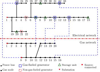
Figure 1: The 33-bus-20-node integrated electrical and gas distribution system.

In the following numerical study, we aim at evaluating the performance of Algorithm 1. We use the 33-bus-20-node network adapted from [18]. An interconnection between the electrical and gas networks occurs when a prosumer (bus) has a gas-fired DG, as illustrated in Figure 1. We generate 100 random test cases where some parameters, such as the gas loads, the locations of generation and storage units, as well as the interconnection points, vary. For each test case, we use the MISOC model and two PWA models with two different numbers of regions, i.e. $r\in\{20,45\}$, thus in total we have 300 instances of the mixed integer game. We perform the simulations in Matlab on a computer with Intel Xeon E5-2637 3.5 GHz processors and 128 GB of memory.

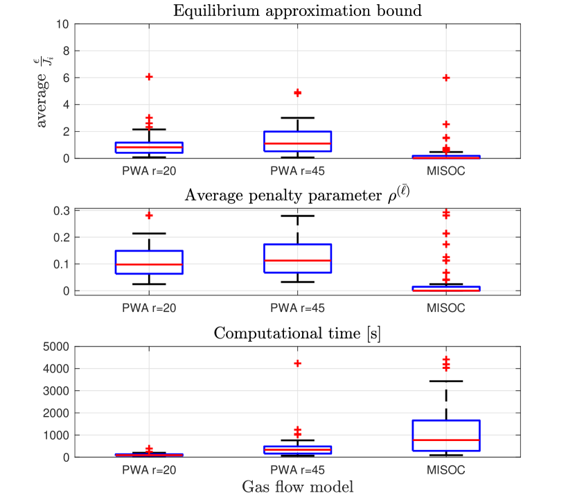
Figure 2: Box plots of the percentage of average $\varepsilon/J_{i}$, the required penalty weight $\rho^{\overline{\ell}}$, and the computational time of Algorithm 1 with different gas flow models.

Figure 2 illustrates the performance of Algorithm 1 with those gas flow models. We obtain the plots from the successful cases, i.e. when Algorithm 1 finds an $\varepsilon$-MIGNE after at most 10 iterations, and they account for approximately $50\%$ of the generated cases. From the top plot of Figure 2, we can observe that Algorithm 1 with the MISOC model produces approximate solutions with the smallest $\varepsilon$. The penalty values, $\rho^{\overline{\ell}}$, required to obtain (approximate) solutions are shown in the middle plot. The bottom plot shows the average computational times of Algorithm 1. As expected, Algorithm 1 needs longer time to find a solution on the PWA model with the larger $r$, as the number of decision variables grow proportionally with $r$. We can also observe that the MISOC model is more computationally demanding than the PWA model with $r=45$.

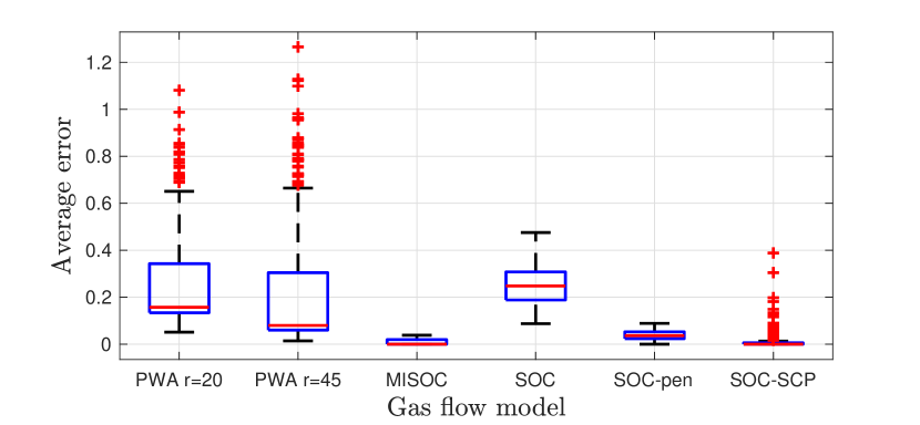
Figure 3: Box plots of the average gas-flow deviations ($\tfrac{1}{H|\mathcal{E}^{\mathrm{g}}|}\sum_{h=1}^{H}\sum_{(i,j)\in\mathcal{E}^{\mathrm{g}}}\Delta^{\phi}_{(i,j),h}$, where $\Delta^{\phi}_{(i,j),h}$ is as in (49)).

Next, we compare the approximation quality of the gas flow models with respect to the Weymouth equation based on the deviation metric derived from (13), i.e.,

$$\small\Delta^{\phi}_{(i,j),h}=\frac{\hat{\phi}_{(i,j),h}-\operatorname{sgn}(\tilde{\psi}_{i,h}-\tilde{\psi}_{j,h})c_{(i,j)}^{\mathrm{f}}\sqrt{|\tilde{\psi}_{i,h}-\tilde{\psi}_{j,h}|}}{\operatorname{sgn}(\tilde{\psi}_{i,h}-\tilde{\psi}_{j,h})c_{(i,j)}^{\mathrm{f}}\sqrt{|\tilde{\psi}_{i,h}-\tilde{\psi}_{j,h}|}},$$ (49)

for all $h\in\mathcal{H}$, $j\in\mathcal{N}_{i}^{\mathrm{g}}$, and $i\in\mathcal{I}$, as shown in Figure 3. As expected, for the PWA model, a larger $r$ implies a smaller deviation, hence a better approximation of the gas-flow constraints. However, the MISOC model outperforms the PWA models as Algorithm 1 with the MISOC model can find a solution that satisfies the Weymouth equation in many of the simulated cases (the case of Proposition 1.(iii) holds). We also compare the two mixed integer models with the standard convex SOC relaxation model, i.e., the MISOC model with fixed binary variables (assuming known gas flow directions) [31, 32], resulting in a jointly convex game. We note that we set the gas flow directions of the convex model based on the solutions of Algorithm 1. Moreover, we implement two approaches to reduce the gas flow deviation of the convex SOC model, namely adding a penalty cost on the auxiliary variable of the SOC model, $\bm{\nu}$, (SOC-pen) [16] and the iterative sequential cone program (SOC-SCP) [31, 16], which requires solving the game at each iteration, as in Algorithm 1. As observed in Figure 3, in terms of the gas flow deviation, the PWA models perform better than the convex SOC relaxation while the MISOC model outperforms the SOC-pen and performs as well as the SOC-SCP.

5 Conclusion

The economic dispatch problem in integrated electrical and gas distribution systems can be formulated as a mixed-integer generalized potential game if the gas-flow equations are approximated by a mixed-integer second order cone (MISOC) or by a piece-wise affine (PWA) model. Our proposed algorithmic solution involves computing a variational equilibrium of the convexified game and leveraging the gas-flow model. An a-posteriori characterization of the outcome of the algorithm is obtained via the evaluation of the potential function. Numerical simulations indicate that our algorithm, particularly if paired with the MISOC model, finds approximate equilibria of very high quality.

6 Gas flow approximation models

In this section, we provide the two commonly considered approximation models of gas-flow equations in (13). For ease of presentation and with a slight abuse of notation, we drop the time index $h$ of each variable.

6.1 Mixed-integer second-order cone model

We summarize the mixed-integer second-order cone relaxation of the gas flow equations in [16] with a reduced number of binary variables. We use the binary variable $\delta_{(i,j)}$ to define the flow direction in the pipeline $(i,j)$, i.e.

$$[\delta_{(i,j)}=1] \Leftrightarrow[\phi_{ij}\geq 0].$$ (50)

resulting in the following constraint:

$$-\overline{\phi}_{(i,j)}(1-\delta_{(i,j)})\leq{\phi}_{(i,j)}\leq\overline{\phi}_{(i,j)}\delta_{(i,j)}.$$ (51)

Consequently, $\delta_{(i,j)}$ also indicates the pressure relationship between two connected nodes $i$ and $j$, i.e.

$$[\delta_{(i,j)}=1] \Leftrightarrow[\psi_{i}\geq\psi_{j}],$$ (52)

Therefore, by squaring (13) and including $\delta_{(i,j)}$, we obtain an equivalent representation of the gas flow equation, as follows:

$$\phi_{(i,j)}^{2}/c_{(i,j)}^{\mathrm{f}}=(2\delta_{(i,j)}-1)(\psi_{i}-\psi_{j}),$$ (53)

for each $j\in\mathcal{N}_{i}^{\mathrm{g}}$ and $i\in\mathcal{I}$.

We use an auxiliary variable, denoted by $\nu_{(i,j)}\in\mathbb{R}^{H}$, to substitute the right-hand-side of (53) and then relax (53) into a convex inequality constraint. Furthermore, by the McCormick envelope, we obtain linear relationships between $\nu_{(i,j)}$, $\delta_{(i,j)}$, $\psi_{i}$ and $\psi_{j}$. As a result, we obtain the following MISOC model:

$$\nu_{(i,j)} \geq\phi_{(i,j)}^{2}/c_{(i,j)}^{\mathrm{f}},$$ (54)

$$\nu_{(i,j)} \geq\psi_{j}-\psi_{i}+2\delta_{(i,j)}(\underline{\psi}_{i}-\overline{\psi}_{j}),$$ (55)

$$\nu_{(i,j)} \geq\psi_{i}-\psi_{j}+(2\delta_{(i,j)}-2)(\overline{\psi}_{i}-\underline{\psi}_{j}),$$ (56)

$$\nu_{(i,j)} \leq\psi_{j}-\psi_{i}+2\delta_{(i,j)}(\overline{\psi}_{i}-\underline{\psi}_{j}),$$ (57)

$$\nu_{(i,j)} \leq\psi_{i}-\psi_{j}+(2\delta_{(i,j)}-2)(\underline{\psi}_{i}-\overline{\psi}_{j}),$$ (58)

for all $j\in\mathcal{N}_{i}^{\mathrm{g}}$ and $i\in\mathcal{I}$.

Therefore, we can compactly represent the local constraints in (51) and (54), for all $j\in\mathcal{N}_{i}^{\mathrm{g}}$, as in (21) and the coupling constraints in (55)–(58), for all $j\in\mathcal{N}_{i}^{\mathrm{g}}$, as in (20). In addition, we also include the reciprocity constraints:

$$\phi_{(i,j)}+\phi_{(j,i)}=0,\quad\forall j\in\mathcal{N}_{i}^{\mathrm{g}},i\in\mathcal{N}^{\mathrm{g}},$$ (59)

for all $j\in\mathcal{N}_{i}^{\mathrm{g}}$, which can be rewritten as in (18). For completeness, we define $h_{i}^{\mathrm{loc}}=0$.

6.2 Piece-wise affine gas-flow model

In this section, we derive a PWA model of the gas-flow equation in (13). First, let us introduce an auxiliary variable $\varphi_{(i,j)}:=\tfrac{\phi_{(i,j)}^{2}}{(c_{(i,j)}^{\mathrm{f}})^{2}}$ and rewrite (13) as follows:

$$\varphi_{(i,j)}=\begin{cases}(\psi_{i}-\psi_{j})\quad\text{if }\psi_{i}\geq\psi_{j},\\ (\psi_{j}-\psi_{i})\quad\text{otherwise.}\end{cases}$$ (60)

Similarly to the MISOC model, we use the binary variable $\delta_{(i,j)}\in\{0,1\}$ to define the flow directions as in (50) and (52). Therefore, we can rewrite (60) as

$$\varphi_{(i,j)} =\delta_{(i,j)}(\psi_{i}-\psi_{j})+(1-\delta_{(i,j)})(\psi_{j}-\psi_{i})$$

$$=2\delta_{(i,j)}\psi_{i}-2\delta_{(i,j)}\psi_{j}+(\psi_{j}-\psi_{i}).$$ (61)

Now, we consider a PWA approximation of the quadratic function $\varphi_{(i,j)}=\tfrac{\phi_{(i,j)}^{2}}{(c_{(i,j)}^{\mathrm{f}})^{2}}$ by partitioning the operating region of the flow into $r$ subregions and introducing a binary variable $\gamma_{(i,j)}^{m}$, for each subregion $m\in\{1,\dots,r\}$, defined by

$$[\gamma_{(i,j)}^{m}=1]\Leftrightarrow[\underline{\phi}_{(i,j)}^{m}\leq\phi_{(i,j)}\leq\overline{\phi}_{(i,j)}^{m}],$$ (62)

with $-\overline{\phi}=\underline{\phi}_{(i,j)}^{1}<\overline{\phi}_{(i,j)}^{1}=\underline{\phi}_{(i,j)}^{2}<\dots<\overline{\phi}_{(i,j)}^{r}=\overline{\phi}$. Then, we can consider the following approximation:

$$\varphi_{(i,j)}\approx\sum_{m=1}^{r}\gamma_{(i,j)}^{m}(a_{(i,j)}^{m}{\phi}_{(i,j)}+b_{(i,j)}^{m}),$$ (63)

for some $a_{(i,j)}^{m},b_{(i,j)}^{m}\in\mathbb{R}$, which can be obtained by using the upper and lower bounds of each subregion, i.e.,

$$a_{(i,j)}^{m}=\tfrac{(\overline{\phi}_{(i,j)}^{m})^{2}-(\underline{\phi}_{(i,j)}^{m})^{2}}{(c_{(i,j)}^{\mathrm{f}})^{2}(\overline{\phi}_{(i,j)}^{m}-\underline{\phi}_{(i,j)}^{m})},\ b_{(i,j)}^{m}=(\underline{\phi}_{(i,j)}^{m})^{2}-a_{(i,j)}^{m}\underline{\phi}_{(i,j)}^{m},$$

for $m=1,\dots,r$. By approximating $\varphi_{(i,j)}$ with (63), we can then rewrite (61) as follows:

$$\sum_{m=1}^{r}\gamma_{(i,j)}^{m}(a_{(i,j)}^{m}{\phi}_{(i,j)}+b_{(i,j)}^{m})=2\delta_{(i,j)}\psi_{i}-2\delta_{(i,j)}\psi_{j}+\psi_{j}-\psi_{i}.$$ (64)

Next, we substitute the products of two variables with some auxiliary variables, i.e., $\nu_{(i,j)}^{m}:=\gamma_{(i,j)}^{m}{\phi}_{(i,j)}$, for $m=1,\dots,r$, and $\nu_{(i,j)}^{\psi}=\delta_{(i,j)}\psi_{i}$. Furthermore, for $j\in\mathcal{N}_{i}^{\mathrm{g}}$, we observe that $\delta_{(i,j)}=1-\delta_{(j,i)},$ and $\delta_{(j,i)}\psi_{j}=\nu_{(j,i)}^{\psi}$, implying that $\delta_{(i,j)}\psi_{j}=(1-\delta_{(j,i)})\psi_{j}=\psi_{j}-\nu_{(j,i)}^{\psi}.$ Thus, from (64), we obtain the following gas-flow equation, for each $(i,j)\in\mathcal{E}^{\mathrm{g}}$:

$$\small\sum_{m=1}^{r}(a_{(i,j)}^{m}\nu_{(i,j)}^{m}+b_{(i,j)}^{m}\gamma_{(i,j)}^{m})=2\nu_{(i,j)}^{\psi}+2\nu_{(j,i)}^{\psi}-\psi_{i}-\psi_{j},$$ (65)

which is linear, involves binary and continuous variables, and couples the decision variables of nodes $i$ and $j$. In addition to (65), we include (51), (59), and the following constraints:

$$\sum_{m=1}^{r}\gamma_{(i,j)}^{m}=1,$$ (66)

since only one subregion can be active;

$$\begin{cases}-\psi_{i}+\psi_{j}\leq-(\underline{\psi}_{i}-\overline{\psi}_{j})(1-\delta_{(i,j)}),\\ -\psi_{i}+\psi_{j}\geq(-(\overline{\psi}_{i}-\underline{\psi}_{j}))\delta_{(i,j)},\end{cases}$$ (67)

which are equivalent to the logical constraint in (52);

$$\begin{cases}\phi_{(i,j)}-\overline{\phi}_{(i,j)}^{m}\leq(\overline{\phi}_{(i,j)}-\overline{\phi}_{(i,j)}^{m})(1-\alpha_{(i,j)}^{m}),\\ \phi_{(i,j)}-\overline{\phi}_{(i,j)}^{m}\geq(-\overline{\phi}_{(i,j)}-\overline{\phi}_{(i,j)}^{m})\alpha_{(i,j)}^{m},\\ -\phi_{(i,j)}+\underline{\phi}_{(i,j)}^{m}\leq(\overline{\phi}_{(i,j)}+\underline{\phi}_{(i,j)}^{m})(1-\beta_{(i,j)}^{m}),\\ -\phi_{(i,j)}+\underline{\phi}_{(i,j)}^{m}\geq(-\overline{\phi}_{(i,j)}+\underline{\phi}_{(i,j)}^{m})\beta_{(i,j)}^{m},\\ -\alpha_{(i,j)}^{m}+\gamma_{(i,j)}^{m}\leq 0,\ \ -\beta_{(i,j)}^{m}+\gamma_{(i,j)}^{m}\leq 0,\\ \alpha_{(i,j)}^{m}+\beta_{(i,j)}^{m}-\gamma_{(i,j)}^{m}\leq 1,\end{cases}$$ (68)

for $m=1,\dots,r$, which are equivalent to the logical constraints (62) [37, Eq. (4e) and (5a)], with $\alpha_{(i,j)}^{m},\beta_{(i,j)}^{m}\in\{0,1\}$, for $m=1,\dots,r,$ being additional binary variables;

$$\small\begin{cases}\nu_{(i,j)}^{m}\geq-\overline{\phi}_{(i,j)}\gamma_{(i,j)}^{m},&\nu_{(i,j)}^{m}\leq\phi_{(i,j)}+\overline{\phi}_{(i,j)}(1-\gamma_{(i,j)}^{m}),\\ \nu_{(i,j)}^{m}\leq\overline{\phi}_{(i,j)}\gamma_{(i,j)}^{m},&\nu_{(i,j)}^{m}\geq\phi_{(i,j)}-\overline{\phi}_{(i,j)}(1-\gamma_{(i,j)}^{m}),\end{cases}$$ (69)

for all $m=1,\dots,r$, which equivalently represent $\nu_{(i,j)}^{m}=\gamma_{(i,j)}^{m}{\phi}_{(i,j)}$ [37, Eq. (5.b)], and;

$$\begin{cases}\nu_{(i,j)}^{\psi}\geq\underline{\psi}_{i}\delta_{(i,j)},\ \ \nu_{(i,j)}^{\psi}\leq\psi_{i}-\underline{\psi}_{i}(1-\delta_{(i,j)}),\\ \nu_{(i,j)}^{\psi}\leq\overline{\psi}_{i}\delta_{(i,j)},\ \ \nu_{(i,j)}^{\psi}\geq\psi_{i}-\overline{\psi}_{i}(1-\delta_{(i,j)}),\end{cases}$$ (70)

which are equivalent to the equality $\nu_{(i,j)}^{\psi_{i}}=\delta_{(i,j)}\psi_{i}$.

Thus, we can compactly write (59) and (65), for all $j\in\mathcal{N}_{i}^{\mathrm{g}}$, as in (18); (66), for all $j\in\mathcal{N}_{i}^{\mathrm{g}}$, as in (19); (67), for all $j\in\mathcal{N}_{i}^{\mathrm{g}}$, as in (20); and (51), (68)–(70), for all $j\in\mathcal{N}_{i}^{\mathrm{g}}$, as in (21).

7 Proofs

7.1 Proof of Lemma 1

Based on the definition of generalized potential games in [38, Def. 2.1], we need to show that (a.) the global feasible set $\bm{\mathcal{U}}$ is non-empty and closed and (b.) the function $P$ in (27) is a potential function of the game in (22). The set $\bm{\mathcal{U}}$, which is non-empty by Assumption 1, is closed since it is constructed from the intersection of closed half spaces and hyperplanes as we have affine non-strict inequality and equality constraints.

Next, by the definition of $J_{i}$ in (23), the pseudogradient mapping of the game in (22) is

$$\operatorname{col}((\nabla_{x_{i}}J_{i}(\bm{x}))):=\operatorname{col}((\nabla_{x_{i}}f_{i}^{\mathrm{loc}}(x_{i}))_{i\in\mathcal{I}})+\bm{D}\bm{x},$$

where $\bm{D}$ is a symmetric matrix, i.e., its block component $(i,j){\in\mathcal{I}\times\mathcal{I}}$ is defined by

$$[\bm{D}]_{i,j}=\begin{cases}2((\Xi_{i}^{\mathrm{e}})^{\top}Q^{\mathrm{e}}\Xi_{i}^{\mathrm{e}}+(\Xi_{i}^{\mathrm{g}})^{\top}Q^{\mathrm{g}}\Xi_{i}^{\mathrm{g}}),&\text{if }i=j,\\ (\Xi_{i}^{\mathrm{e}})^{\top}Q^{\mathrm{e}}\Xi_{j}^{\mathrm{e}}+(\Xi_{i}^{\mathrm{g}})^{\top}Q^{\mathrm{g}}\Xi_{j}^{\mathrm{g}},&\text{otherwise.}\end{cases}$$

On the other hand, by the definition of $P$ in (27), it holds that

$$P(\bm{x})= \tfrac{1}{2}\sum_{i\in\mathcal{I}}(J_{i}(\bm{x})+f_{i}^{\mathrm{loc}}(x_{i})+x_{i}^{\top}D_{i}x_{i}))$$

$$= \sum_{i\in\mathcal{I}}(f_{i}^{\mathrm{loc}}(x_{i}))+\tfrac{1}{2}(x_{i}^{\top}D_{i}x_{i}+f_{i}^{\mathrm{cpl}}(\bm{x})))$$

$$= \sum_{i\in\mathcal{I}}f_{i}^{\mathrm{loc}}(x_{i})+\tfrac{1}{2}\bm{x}^{\top}\bm{D}\bm{x}.$$

Thus, $\nabla_{\bm{x}}P(\bm{x})=\operatorname{col}((\nabla_{x_{i}}J_{i}(\bm{x}))_{i\in\mathcal{I}})$, implying that $P$ is an exact potential function of the game in (22).

7.2 Proof of Lemma 2

1. We have that

   $$\operatorname{col}((\nabla_{x_{i}}J_{i}(\bm{x}))):=\operatorname{col}((\nabla_{x_{i}}f_{i}^{\mathrm{loc}}(x_{i}))_{i\in\mathcal{I}})+\bm{D}\bm{x},$$

   where $\bm{D}$ is as defined in the proof of Lemma 1. The operator $\operatorname{col}((\nabla_{x_{i}}f_{i}^{\mathrm{loc}}(x_{i}))_{i\in\mathcal{I}})$ is monotone since it is a concatenation of monotone operators $\nabla_{x_{i}}f_{i}^{\mathrm{loc}}(x_{i}))$, for all $i\in\mathcal{I}$, [41, Prop. 20.23] as $f_{i}^{\mathrm{loc}}$, for each $i\in\mathcal{I}$, is differentiable and convex by definition. Furthermore, $\bm{D}$ is positive semidefinite by construction. Therefore, both $\operatorname{col}((\nabla_{x_{i}}J_{i}(\bm{x}))_{i\in\mathcal{I}})$ and $F$, which concatenates $\operatorname{col}(\nabla_{x_{i}}J_{i}(\bm{x}))_{i\in\mathcal{I}})$ and $\mathbf{0}$, are monotone.

2. As in the proof of Lemma 1, $\nabla_{\bm{x}}P(\bm{x})=\operatorname{col}((\nabla_{x_{i}}J_{i}(\bm{x}))_{i\in\mathcal{I}})$, which is monotone by Lemma 2.(i). Hence, $P$ is a convex function.

7.3 Proof of Proposition 1

1. Since $\hat{\bm{u}}$ is a feasible point of the convexified game in (31), then $\hat{\bm{u}}$ satisfies all the constraints in the original game (22) except possibly the integrality constraints $z_{i}\in\{0,1\}^{n_{z_{i}}}$, for all $i\in\mathcal{I}$. Therefore, by construction, $\bm{u}^{\star}=(\bm{x}^{\star},\bm{y}^{\star},\bm{z}^{\star})$ satisfies all the constraints but the MISOC gas flow constraints (55)–(58), equivalently (35). By the definition of the inequality constraints (37b), a solution to Problem (37) satisfies (35) if and only if $\tilde{\bm{\tau}}=\mathbf{0}$.

2. From point (i), $\bm{u}^{\star}$ is a feasible point of the original game if and only if $\tilde{\bm{\tau}}=\mathbf{0}$. Furthermore, we observe that the cost functions in the original game (22) and those in the convexified game (31) are equal and only depend on $\bm{x}$. By considering that $\hat{\bm{u}}$ is a variational GNE of the game in (31), implying that it is also a solution to Problem (32), and that the optimal value of Problem (32) is a lower bound of Problem (30), we can conclude that $\bm{u}^{\star}$ is a solution to Problem (30) as $P(\bm{u}^{\star})=P(\hat{\bm{u}})$. Hence, $\bm{u}^{\star}$ is an exact GNE of the original game, i.e., the inequality in (29) holds with $\varepsilon=0$ [27, Thm 2].

3. When $J_{\psi}(\tilde{\bm{\psi}})=0$, which also consequently implies that $\|\tilde{\tau}\|_{\infty}=0$, the SOC gas flow constraint $\nu_{(i,j)}\geq\phi_{(i,j)}^{2}/c_{(i,j)}^{\mathrm{f}}$, for each $(i,j)\in\mathcal{E}^{\mathrm{g}}$, is tight, i.e., satisfied with an equality.

7.4 Proof of Lemma 3

A set of solutions to (40) exists if and only if $\operatorname{rank}\left(\begin{bmatrix}E(\tilde{\bm{\delta}}_{h})&\bm{\theta}_{h}(\hat{\bm{\phi}_{h}})\end{bmatrix}\right)=\operatorname{rank}(E(\tilde{\bm{\delta}}_{h}))$, for all $h\in\mathcal{H}$. Since we assume $\mathcal{G}^{\mathrm{g}}$ is connected, $\mathcal{G}^{\mathrm{g}}$ is either a minimum tree or is not a minimum tree. When $\mathcal{G}^{\mathrm{g}}$ is a minimum tree, $|\mathcal{E}^{\mathrm{g}}|=2(N-1)$, as we label an edge between node $i$ and $j$ twice, i.e. $(i,j)$ and $(j,i)$. Therefore, $\operatorname{rank}(E(\tilde{\bm{\delta}}_{h}))=N-1$. Moreover, $\begin{bmatrix}E(\tilde{\bm{\delta}}_{h})&\bm{\theta}_{h}(\hat{\bm{\phi}_{h}})\end{bmatrix}\in\mathbb{R}^{|\mathcal{E}^{\mathrm{g}}|\times(N+1)}$ and $\phi_{(i,j),h}^{2}=\phi_{(j,i),h}^{2}$, for all $(i,j)\in\mathcal{E}^{\mathrm{g}}$. Thus, $\operatorname{rank}\left(\begin{bmatrix}E(\tilde{\bm{\delta}}_{h})&\bm{\theta}_{h}(\hat{\bm{\phi}_{h}})\end{bmatrix}\right)=N-1$.

7.5 Proof of Theorem 1

By Lemma 2.(ii), $P(\bm{x})$ in (27) is a convex function. Therefore, a variational GNE of the convexified game in (42) with $\rho=\rho^{(1)}=0$ (or equivalently the game in (31)), denoted by $(\hat{\bm{x}}^{(\ell)},\hat{\bm{y}}^{(\ell)},\hat{\bm{z}}^{(\ell)})$, is a solution to Problem (32), which is a convex relaxation of Problem (30). Therefore, by denoting with $\bm{u}^{\ast}=(\bm{x}^{\ast},\bm{y}^{\ast},\bm{z}^{\ast})$ a solution to Problem (30), which is an exact GNE of the game in (22), we have that

$$P(\tilde{\bm{x}}^{(1)})=P(\hat{\bm{x}}^{(1)})\leq P(\bm{x}^{\ast}),$$ (71)

where the equality holds since $\tilde{\bm{x}}^{(\ell)}=\hat{\bm{x}}^{(\ell)}$ (see Step 4 of Algorithm 1). Next, we observe from Proposition 1.(i) that $\tilde{\bm{u}}^{(\overline{\ell})}$ is a feasible point but is not necessarily a solution to Problem (32) (nor a GNE) since the cost functions considered in Step 1 is $\tilde{J}_{i}$, for all $i\in\mathcal{I}$. Thus, it holds that

$$P(\bm{x}^{\ast})\leq P(\tilde{\bm{x}}^{(\overline{\ell})}).$$ (72)

Since $P$ is an exact potential function, it holds that, for each $i\in\mathcal{I}$ and any $(x_{i},y_{i},z_{i})\in\mathcal{L}_{i}\cap\mathcal{C}_{i}(\tilde{\bm{u}}_{-i}^{(\overline{\ell})})\cap\mathbb{R}^{n_{x_{i}}+n_{y_{i}}}\times\{0,1\}^{n_{z_{i}}}$, we have that

$$J_{i}(\tilde{\bm{x}}^{(\overline{\ell})})-J_{i}(x_{i},\tilde{\bm{x}}_{-i}^{(\overline{\ell})}) =P(\tilde{\bm{x}}^{(\overline{\ell})})-P(x_{i},\tilde{\bm{x}}_{-i}^{(\overline{\ell})})$$

$$\leq P(\tilde{\bm{x}}^{(\overline{\ell})})-P(\bm{x}^{\ast})$$

$$\leq P(\tilde{\bm{x}}^{(\overline{\ell})})-P(\tilde{\bm{x}}^{(1)})=\varepsilon,$$

where the first inequality holds since $\bm{u}^{\ast}$ is an optimizer of Problem (30), and the second inequality is obtained by combining (71) and (72).

7.6 Proof of Proposition 2

By the definition of the matrix $E(\tilde{\bm{\delta}}_{h})$ and Assumption 2, its null space is $\{\mathbf{1}_{N}\}$. Hence, for each $h\in\mathcal{H}$, the solutions to (47) can be described by $\bm{\psi}_{h}^{0}+\xi\mathbf{1}_{N},$ for any $\xi\in\mathbb{R}$. Therefore, Problem (45) has at least a solution if and only if there exists $\xi\in\mathbb{R}$ such that

$$\operatorname{col}(\{\underline{\psi}_{i}\}_{i\in\mathcal{I}})\leq\bm{\psi}_{h}^{0}+\xi\mathbf{1}_{N}\leq\operatorname{col}(\{\overline{\psi}_{i}\}_{i\in\mathcal{I}}),$$ (73)

since for any $\xi\in\mathbb{R}$, $J_{\psi}(\bm{\psi}_{h}^{0}+\xi\mathbf{1}_{N})=0$. For each $h\in\mathcal{H}$, let us now consider another particular solution,

$$\bar{\bm{\psi}}_{h}^{0}=\bm{\psi}_{h}^{0}-\mathbf{1}_{N}\min_{i\in\mathcal{I}}[\bm{\psi}_{h}^{0}]_{i},$$ (74)

i.e., $\xi=-\min_{i\in\mathcal{I}}[\bm{\psi}_{h}^{0}]_{i}$. Hence, $\min_{i\in\mathcal{I}}[\bar{\bm{\psi}}_{h}^{0}]_{i}=0$ and $\max_{i\in\mathcal{I}}[\bar{\bm{\psi}}_{h}^{0}]_{i}=\max_{i\in\mathcal{I}}[{\bm{\psi}}_{h}^{0}]_{i}-\min_{i\in\mathcal{I}}[\bm{\psi}_{h}^{0}]_{i}\geq 0$. Now, let us consider the indices $j$ and $k$ as defined in Proposition 2, i.e., $j\in\operatorname{argmin}_{\ell\in\operatorname{argmax}_{i\in\mathcal{I}}[\bm{\psi}_{h}^{0}]_{i}}\overline{\psi}_{\ell}$, and $k\in\operatorname{argmax}_{\ell\in\operatorname{argmin}_{i\in\mathcal{I}}[\bm{\psi}_{h}^{0}]_{i}}\overline{\psi}_{\ell}$ and let us substitute $\bm{\psi}_{h}^{0}$ with $\bar{\bm{\psi}}_{h}^{0}$ in (73). Since $\underline{\psi}_{i}\geq 0$, for any $i\in\mathcal{I}$, and $\min_{i\in\mathcal{I}}[\bar{\bm{\psi}}_{h}^{0}]_{i}=0$, the first inequality in (73) is satisfied if and only if $\xi\geq\underline{\psi}_{k}\geq 0$. Furthermore, the second inequality is satisfied if and only if $\xi\leq\overline{\psi}_{j}-[\bar{\bm{\psi}}_{h}^{0}]_{j}$. Hence, there exists $\xi\geq 0$ if and only if

$$\underline{\psi}_{k}\leq\overline{\psi}_{j}-[\bar{\bm{\psi}}_{h}^{0}]_{j} \Leftrightarrow[\bar{\bm{\psi}}_{h}^{0}]_{j}\leq\overline{\psi}_{j}-\underline{\psi}_{k}$$

$$\Leftrightarrow[\bm{\psi}_{h}^{0}]_{j}-[\bm{\psi}_{h}^{0}]_{k}\leq\overline{\psi}_{j}-\underline{\psi}_{k},$$

where the last implication follows the definition of $\bar{\bm{\psi}}_{h}^{0}$ in (74).

References

• [1] G. Pepermans, J. Driesen, D. Haeseldonckx, R. Belmans, and W. D’haeseleer, “Distributed generation: Definition, benefits and issues,” Energy policy, vol. 33, no. 6, pp. 787–798, 2005.
• [2] L. Mehigan, J. P. Deane, B. Ó. Gallachóir, and V. Bertsch, “A review of the role of distributed generation (DG) in future electricity systems,” Energy, vol. 163, pp. 822–836, 2018.
• [3] M. Houwing, R. R. Negenborn, and B. De Schutter, “Demand response with micro-CHP systems,” Proc. of the IEEE, vol. 99, no. 1, pp. 200–213, 2010.
• [4] G. Zhang, Z. Shen, and L. Wang, “Online energy management for microgrids with CHP co-generation and energy storage,” IEEE Trans. Control Systems Technology, vol. 28, no. 2, pp. 533–541, 2020.
• [5] A. Zlotnik, L. Roald, S. Backhaus, M. Chertkov, and G. Andersson, “Control policies for operational coordination of electric power and natural gas transmission systems,” in Proc. of American Control Conference, 2016, pp. 7478–7483.
• [6] M. K. Singh and V. Kekatos, “Natural gas flow solvers using convex relaxation,” IEEE Trans. Control of Network Systems, vol. 7, no. 3, pp. 1283–1295, 2020.
• [7] K. Sundar, S. Misra, A. Zlotnik, and R. Bent, “Robust gas pipeline network expansion planning to support power system reliability,” in Proc. American Control Conference, 2021, pp. 620–627.
• [8] S. K. K. Hari, K. Sundar, S. Srinivasan, A. Zlotnik, and R. Bent, “Operation of natural gas pipeline networks with storage under transient flow conditions,” IEEE Trans. Control Systems Technology, vol. 30, no. 2, pp. 667–679, 2022.
• [9] L. A. Roald, K. Sundar, A. Zlotnik, S. Misra, and G. Andersson, “An uncertainty management framework for integrated gas-electric energy systems,” Proc. of the IEEE, vol. 108, no. 9, pp. 1518–1540, 2020.
• [10] M. Urbina and Z. Li, “A combined model for analyzing the interdependency of electrical and gas systems,” in 2007 39th North American power symposium.   IEEE, 2007, pp. 468–472.
• [11] C. M. Correa-Posada and P. Sánchez-Martın, “Security-constrained optimal power and natural gas flow,” IEEE Trans. Power Systems, vol. 29, no. 4, pp. 1780–1787, 2014.
• [12] X. Zhang, M. Shahidehpour, A. Alabdulwahab, and A. Abusorrah, “Hourly electricity demand response in the stochastic day-ahead scheduling of coordinated electricity and natural gas networks,” IEEE Trans. Power Systems, vol. 31, no. 1, pp. 592–601, 2015.
• [13] G. Wu, Y. Xiang, J. Liu, J. Gou, X. Shen, Y. Huang, and S. Jawad, “Decentralized day-ahead scheduling of multi-area integrated electricity and natural gas systems considering reserve optimization,” Energy, vol. 198, p. 117271, 2020.
• [14] Y. He, M. Shahidehpour, Z. Li, C. Guo, and B. Zhu, “Robust constrained operation of integrated electricity-natural gas system considering distributed natural gas storage,” IEEE Trans. Sustainable Energy, vol. 9, no. 3, pp. 1061–1071, 2017.
• [15] Y. Wen, X. Qu, W. Li, X. Liu, and X. Ye, “Synergistic operation of electricity and natural gas networks via ADMM,” IEEE Trans. Smart Grid, vol. 9, no. 5, pp. 4555–4565, 2017.
• [16] Y. He, M. Yan, M. Shahidehpour, Z. Li, C. Guo, L. Wu, and Y. Ding, “Decentralized optimization of multi-area electricity-natural gas flows based on cone reformulation,” IEEE Trans. Power Systems, vol. 33, no. 4, pp. 4531–4542, 2017.
• [17] F. Liu, Z. Bie, and X. Wang, “Day-ahead dispatch of integrated electricity and natural gas system considering reserve scheduling and renewable uncertainties,” IEEE Trans. Sustainable Energy, vol. 10, no. 2, pp. 646–658, 2018.
• [18] Y. Li, Z. Li, F. Wen, and M. Shahidehpour, “Privacy-preserving optimal dispatch for an integrated power distribution and natural gas system in networked energy hubs,” IEEE Trans. Sustainable Energy, vol. 10, no. 4, pp. 2028–2038, 2018.
• [19] F. Qi, M. Shahidehpour, Z. Li, F. Wen, and C. Shao, “A chance-constrained decentralized operation of multi-area integrated electricity–natural gas systems with variable wind and solar energy,” IEEE Trans. Sustainable Energy, vol. 11, no. 4, pp. 2230–2240, 2019.
• [20] I. Atzeni, L. G. Ordóñez, G. Scutari, D. P. Palomar, and J. R. Fonollosa, “Demand-side management via distributed energy generation and storage optimization,” IEEE Trans. Smart Grid, vol. 4, no. 2, pp. 866–876, 2013.
• [21] G. Belgioioso, W. Ananduta, S. Grammatico, and C. Ocampo-Martinez, “Operationally-safe peer-to-peer energy trading in distribution grids: A game-theoretic market-clearing mechanism,” IEEE Trans. Smart Grid, vol. 13, no. 4, pp. 2897–2907, 2022.
• [22] F. Facchinei and C. Kanzow, “Generalized Nash equilibrium problems,” Annals of Operations Research, vol. 175, no. 1, pp. 177–211, 2010.
• [23] P. Yi and L. Pavel, “An operator splitting approach for distributed generalized Nash equilibria computation,” Automatica, vol. 102, pp. 111–121, 2019.
• [24] B. Franci, M. Staudigl, and S. Grammatico, “Distributed forward-backward (half) forward algorithms for generalized Nash equilibrium seeking,” in Proc. 2020 European Control Conference (ECC).   IEEE, 2020, pp. 1274–1279.
• [25] G. Belgioioso and S. Grammatico, “Semi-decentralized generalized Nash equilibrium seeking in monotone aggregative games,” IEEE Trans. Automatic Control, 2021.
• [26] M. Bianchi, G. Belgioioso, and S. Grammatico, “Fast generalized nash equilibrium seeking under partial-decision information,” Automatica, vol. 136, p. 110080, 2022.
• [27] S. Sagratella, “Algorithms for generalized potential games with mixed-integer variables,” Computational Optimization and Applications, vol. 68, no. 3, pp. 689–717, 2017.
• [28] ——, “On generalized Nash equilibrium problems with linear coupling constraints and mixed-integer variables,” Optimization, vol. 68, no. 1, pp. 197–226, 2019.
• [29] C. Cenedese, F. Fabiani, M. Cucuzzella, J. M. A. Scherpen, M. Cao, and S. Grammatico, “Charging plug-in electric vehicles as a mixed-integer aggregative game,” in Proc. IEEE 58th Conference on Decision and Control (CDC), 2019, pp. 4904–4909.
• [30] F. Fabiani and S. Grammatico, “Multi-vehicle automated driving as a generalized mixed-integer potential game,” IEEE Trans. Intelligent Transportation Systems, vol. 21, no. 3, pp. 1064–1073, 2020.
• [31] C. Wang, W. Wei, J. Wang, L. Wu, and Y. Liang, “Equilibrium of interdependent gas and electricity markets with marginal price based bilateral energy trading,” IEEE Trans. Power Systems, vol. 33, no. 5, pp. 4854–4867, 2018.
• [32] S. Chen, A. J. Conejo, R. Sioshansi, and Z. Wei, “Operational equilibria of electric and natural gas systems with limited information interchange,” IEEE Trans. Power Systems, vol. 35, no. 1, pp. 662–671, 2020.
• [33] A. Falsone, K. Margellos, and M. Prandini, “A distributed iterative algorithm for multi-agent milps: Finite-time feasibility and performance characterization,” IEEE Control Systems Letters, vol. 2, no. 4, pp. 563–568, 2018.
• [34] A. Camisa and G. Notarstefano, “A distributed mixed-integer framework to stochastic optimal microgrid control,” IEEE Trans. Control Systems Technology, pp. 1–13, 2022.
• [35] W. Ananduta and S. Grammatico, “Approximate solutions to the optimal flow problem of multi-area integrated electrical and gas systems,” in Proc. the 61st Conference on Decision and Control, 2022, to appear, available at https://arxiv.org/abs/2206.01098.
• [36] Z. Yang, K. Xie, J. Yu, H. Zhong, N. Zhang, and Q. Xia, “A general formulation of linear power flow models: Basic theory and error analysis,” IEEE Trans. Power Systems, vol. 34, no. 2, pp. 1315–1324, 2019.
• [37] A. Bemporad and M. Morari, “Control of systems integrating logic, dynamics, and constraints,” Automatica, vol. 35, no. 3, pp. 407–427, 1999.
• [38] F. Facchinei, V. Piccialli, and M. Sciandrone, “Decomposition algorithms for generalized potential games,” Computational Optimization and Applications, vol. 50, no. 2, pp. 237–262, 2011.
• [39] A. Falsone, K. Margellos, S. Garatti, and M. Prandini, “Dual decomposition for multi-agent distributed optimization with coupling constraints,” Automatica, vol. 84, pp. 149–158, 2017.
• [40] W. Ananduta, A. Nedić, and C. Ocampo-Martinez, “Distributed augmented lagrangian method for link-based resource sharing problems of multiagent systems,” IEEE Trans. Automatic Control, vol. 67, no. 6, pp. 3067–3074, 2022.
• [41] H. H. Bauschke and P. L. Combettes, Convex analysis and monotone operator theory in Hilbert spaces.   Springer, 2011, vol. 408.