A common lines approach for ab-initio modeling of molecules with tetrahedral and octahedral symmetry
Abstract
A main task in cryo-electron microscopy single particle reconstruction is to find a three-dimensional model of a molecule given a set of its randomly oriented and positioned noisy projection-images. In this work, we propose an algorithm for ab-initio reconstruction for molecules with tetrahedral or octahedral symmetry. The algorithm exploits the multiple common lines between each pair of projection-images as well as self common lines within each image. It is robust to noise in the input images as it integrates the information from all images at once. The applicability of the proposed algorithm is demonstrated using experimental cryo-electron microscopy data.
Adi Shasha Geva
Department of Applied Mathematics, School of Mathematical Sciences
Tel-Aviv University
shashaadi@gmail.com
Yoel Shkolnisky
Department of Applied Mathematics, School of Mathematical Sciences
Tel-Aviv University
yoelsh@tauex.tau.ac.il
Please address manuscript correspondence to Adi Shasha Geva, shashaadi@gmail.com
1 Introduction
Cryo-electron microscopy (cryo-EM) is a method for determining the high-resolution three-dimensional structure of biomolecules [5]. The method involves imaging frozen copies of the investigated molecule by an electron-microscope, with each copy assuming some unknown random orientation fixed at the moment of freezing. Due to the low electron dose that can be applied to the imaged molecules, the projection-images produced by cryo-EM are very noisy. Once the orientation of each of the imaged copies of the molecule has been determined, a low-resolution ab-initio model of the molecule may be recovered from the acquired projection-images by tomographic reconstruction algorithms. An accurate ab-initio model is crucial for obtaining a high-resolution model, which is determined by iterative procedures from the set of raw input projection-images. The task of finding the orientation of the molecule giving rise to each projection-image is known as the “orientation assignment problem”, and is the main objective of this work.
Formally, if we denote the electrostatic potential of the molecule by , and consider a set of rotation matrices
| (1) |
where is the group of all rotations in , then the projection-image , , that was generated by imaging rotated by , is given by the line integrals of along the lines parallel to (the third column of ), namely
| (2) |
The “orientation assignment problem” is defined as finding a set of rotation matrices such that (2) holds for all , given only the set of projection-images .
An inherent ambiguity in cryo-electron microscopy stems from the fact that the handedness (chirality) of the molecule cannot be resolved from its projection-images. This ambiguity is referred to as the handedness ambiguity. Consequently, any projection-image is compatible with two distinct orientations as follows. We denote by the reflection matrix through the -plane, and define by the mirror image of the molecule , . Since , , and along with (2) we have
By noting that and using the change of variables we have
| (3) |
where is a projection-image generated from . Equation (3) shows that a projection-image of the molecule at orientation is identical to a projection-image of its mirror image molecule at orientation . Thus, both sets of orientations assignments and are consistent with the same set of projection-images . Biologically, only the model reconstructed using the orientations is valid, yet distinguishing whether a reconstruction corresponds to or is impossible without utilizing other structural information.
In this work, we propose an algorithm for solving the “orientation assignment problem” for molecules with tetrahedral or octahedral symmetry [6], denoted by and , respectively. To present these symmetries, we denote by the group of all rotations by radians around some fixed axis (rotational symmetry of order ). Then, the elements of the tetrahedral symmetry group are the identity, the elements of 4 rotation groups whose axes pass through each vertex of the regular tetrahedron (see Fig. 1) and the corresponding midpoint of the opposite face, and the elements of 3 rotation groups whose axes pass through the midpoints of two of its opposite edges. In total, the tetrahedral group has 12 elements. The elements of the octahedral symmetry group are the identity, the elements of 3 rotation groups whose axes pass through two opposite vertices of the regular octahedron (see Fig. 1), 4 rotation groups whose axes pass through the midpoints of two of its opposite faces, and 6 rotation groups whose axe pass through the midpoints of two of its opposite edges. In total, the octahedral group has 24 elements.
Since the structure of a molecule is independent of its coordinate system, we choose without loss of generality a coordinate system in which the rotational axes mentioned above coincide with the axes listed in Table 1. In this coordinate system, the symmetry group elements of a molecule with tetrahedral symmetry are given in Appendix A.1 and the symmetry group elements of a molecule with octahedral symmetry are given in Appendix A.2.
| symmetry | axes | angles |
| [1,1,1], [-1,-1,1], [-1,1,-1], [1,-1,-1] | , | |
| [1,0,0], [0,1,0], [0,0,1] | ||
| [1,0,0], [0,1,0], [0,0,1] | , , | |
| [1,1,1], [-1,1,1], [1,-1,1], [1,1,-1] | , | |
| [1,1,0], [-1,1,0], [1,0,1], [-1,0,1], [0,1,1], [0,-1,1] |
To see the effect of symmetry on the orientation assigment problem, we denote by the -th symmetry group element of the symmetry group or , , where is the number of elements in the symmetry group. Mathematically, a molecule has symmetry ( or ) if
| (4) |
for any . Together with (2), it holds that for any and any ,
| (5) |
for all , implying that the projection-images are identical. Hence, equation (5) reveals another ambiguity of the set of projection-images , referred to as the symmetry ambiguity, in which all orientation assignments of the form , where is an arbitrary symmetry group element, are consistent with the same set of images .
Combining the symmetry ambiguity with the handedness ambiguity described in (3), the orientation assignment problem can be stated as finding either one of the sets of orientations or , where each may be replaced by , with being an arbitrary symmetry group element, independently for each (that is independently for each rotation).
Solving the orientation assignment problem, in its broadest sense, amounts to relating between images and rotation matrices. In this work, we introduce a common lines based method for solving the orientation assignment problem for molecules having either tetrahedral or octahedral symmetry. The common lines, defined in the following and discussed in detail in subsequent sections, reveal useful relations between images and rotation matrices. To define common lines, we recall the Fourier projection slice theorem [9], which provides an important relation between the Fourier transform of and the Fourier transform of (see (2)). We define the two-dimensional Fourier transform of a projection-image (2) by
and the three-dimensional Fourier transform of the molecule by
Using this notation, the Fourier projection slice theorem states that
| (6) |
where and are the first and second columns of , respectively. In words, the two-dimensional Fourier transform of any projection-image is equal to the restriction of the three-dimensional Fourier transform of the molecule to the plane through the origin spanned by and , or equivalently, to the central plane whose normal coincides with . As any two central planes intersect along a single line through the origin (as long as the central planes do not coincide), the central planes corresponding to any pair of Fourier-transformed projection-images and intersect along such a line, and therefore, both (Fourier transformed) images share a pair of lines on which their Fourier transforms coincide, thus referred to as common lines. Given that and are images of a molecule with tetrahedral or octahedral symmetry, each , , is identical to (see (5)). In addition, each , , also shares a common line with . Since the rotations , , are in general different from each other, the planes spanned by their first two columns are also different. Thus, and have common lines altogether.
2 Related work
Common lines methods for ab-initio reconstruction of macromolecules have originated with the angular reconstitution method by Van Heel [23]. It is a sequential method in which given a triplet of projection-images , the set of relative rotations is first estimated by detecting common lines between and . Then, setting without loss of generality, determines and from and . By applying this method sequentially to each triplet where , the orientation of the image is determined from simply by .
Detecting common lines between a pair of images is typically done by finding the pair of central lines in the Fourier transforms of the images that have the highest correlation [19]. In cryo-EM, the images are contaminated with high levels of noise, thus making the detection of common lines error prone. Consequently, the relative rotations in the angular reconstitution method are estimated with errors, which render the method not robust to noise.
A common lines based approach for molecules without symmetry that is robust to noisy input images is the synchronization method [17, 11]. In this approach, all relative rotations are first estimated using common lines (robust estimation of common lines is described in [19, 7]). Then, the rotations are estimated simultaneously, by constructing a matrix whose block of size contains the estimate for , and factorizing this matrix using SVD. However, this method is not applicable to symmetric molecules due to the symmetry ambiguity described by (5). Specifically, consider a pair of images and , , of a molecule with tetrahedral or octahedral symmetry. By the discussion above, there are pairs of common lines between the images, corresponding to pairs of projection planes, but it is unknown which pair of common lines corresponds to which pair of projection planes. As a result, the best one can estimate from a single pair of common lines between the images is the relative rotation , where is an unknown arbitrary symmetry group element. In such a case, factorizing the matrix whose blocks are does not give (more precisely for some arbitrary ), unless we are able to carefully choose .
Two robust common lines based methods which are applicable to symmetric molecules are described in [12] for molecules with symmetry and in [16] for molecules with symmetry. In both methods, all common lines between each pair of images are utilized to estimate a set , with being an unknown symmetry group element of the or symmetry groups. Once the set has been estimated, the methods exploit the symmetry group properties to obtain the set of rotation matrices , with each rotation matrix satisfying . Unfortunately, the methods in [12, 16] are not applicable to molecules with or symmetries. Specifically, the method in [12] for molecules with symmetry uses the property that the average of the group elements of is the matrix . This property doesn’t hold for molecules with or symmetry, as the average over all group elements of the groups and is the zero matrix. As for the method in [16] for molecules with symmetry, this method assumes that the rotational symmetry axes of the molecule coincide with the and axes, which does not hold for and symmetries.
While we propose a method that is based on common lines, there exist algorithms for finding ab-initio models that are based on casting the reconstruction problem as an optimization problem [13, 26, 22, 3]. Such algorithms use some general-purpose optimization algorithm (such as stochastic gradient descent, stochastic hill climbing, projection-matching, and simulated annealing, to name a few), on a subset of the data or its class averages. All these methods boil down to a non-convex optimization, which is susceptible to getting stuck in a local minimum corresponding to a structure that is inconsistent with the investigated molecule. Yet, these methods are widely used in practice and many times produce satisfactory initial models. In Section 5 we show an example of both a success as well as a failure of such a method.
The paper is organized as follows. In Section 3, we formally define the common lines, introduce the notion of self common lines and derive basic properties of common lines and self common lines. In Section 4, we describe our algorithm for estimating the orientations of a given set of projection-images. Then, in Section 5, we report some numerical experiments we conducted using simulated and experimental data sets, demonstrating the robustness and effectiveness of our proposed method. Finally, in Section 6, we discuss possible future work.
3 Common lines and self common lines
Formally, for each , the unit vector
| (7) |
gives the direction of the common line between the central planes of and , since it is perpendicular to the normal vectors of both of them. We can express using its local coordinates on both central planes by
| (8) |
where and are the angles between and the local -axes of the planes. Using this notation along with (6), we have that for any and ,
| (9) |
Following (9), we express the set of common lines between the pair of images and by the set of local coordinates . In particular, and may be recovered from the entries of using
| (10) |
Note that in (7), the vector is multiplied by the symmetry group element , , while is not. Since this choice is arbitrary, we show in the following that we get the same common lines if we multiply by instead. In other words, we show in the following that the set of local coordinates for the common lines between the pair of images and is well defined.
Similarly to (7), for each , the unit vector
| (11) |
gives the direction of the common line between the central planes of the Fourier transformed images and . As is a group, for each there is such that . Then, using (7), it holds that
| (12) |
where the second equality follows since for any rotation it holds that , and the third equality follows from the latter property along with the anti-commutative property of the cross product, i.e., , and the invariance of the 2-norm to orthogonal transformations. By multiplying (8) by from the left we get using (12)
| (13) |
Equation (13) implies that and are also the angles between and the local -axes of the planes of the Fourier transformed images and . Then, similarly to (9),
| (14) |
Thus, the set of local coordinates for the common lines is well defined, as the same set is obtained from the two equivalent definitions (7) and (11).
Another important property of projection-images of symmetric molecules, and in particular of molecules with tetrahedral or octahedral symmetry, is the existence of self common lines, which are common lines between any two (identical) images and , . The direction vector of the self common line between and is
| (15) |
When expressing by the local coordinates , we get similarly to (9) that
| (16) |
and and may be recovered from the entries of using
| (17) |
Thus, the set of self common lines of the image is expressed by the set of local coordinates .
4 Algorithm
In this section, we derive our method for solving the orientation assignment problem for molecules with tetrahedral or octahedral symmetry. Throughout this section, we denote by either the group or the group . Our method consists of two steps; first, we assign to each pair of projection-images and (see (2)) , , of a molecule whose symmetry group is , a pair of rotation matrices which is an estimate to a pair of rotation matrices which satisfies
| (18) |
Then, we estimate the orientations of all projection-images from the set of rotation matrices .
To find the rotations and which estimate and of (18), we follow the maximum likelihood approach described in [12, 16] as follows. First, we construct a function , which for any two rotations computes a score that indicates how well approximates . Since it is impossible to find efficiently the optimum of over , we show in Appendix C how to construct a finite subset on which we search for the optimum of . In particular, the subset takes advantage of the fact that the underlying molecule is symmetric, to reduce the number of rotations in , while maintaining high accuracy of our algorithm. We use the pair that attains the highest score as our estimate for of (18).
We next describe the construction of the function for each pair of images and . We denote by
| (19) |
the half line (known as a Fourier ray) in the direction which forms an angle with the -axis of the Fourier transformed image , , and by
| (20) |
the real part of the normalized cross correlations between and . Note that due to (9), it holds that for all , where is the set of common lines between and .
Now, consider a pair of rotations . Analogously to (10), we compute the set of local coordinates from the set using
| (21) |
If , then (21) along with (10) imply that the set of local coordinates is the set of common lines of the pair of images and , i.e, it is equal to . The score function is thus defined as
| (22) |
satisfying if . We note that we define in (22) as a product to enforce that all correlations are large simultaneously. Each is a proxy to the probability that is a common line between and , and we want all these probabilities to be large simultaneously.
In practice, since is computed using noisy images, and since is only a finite subset of , is unlikely to be exactly 1. Thus, the pair of candidates with the highest score is used to construct , which serves as an estimate for .
In order to achieve a more robust estimate of , we also combine the set of self common lines into the score function of (22). Specifically, as and are the sets of self common lines of and respectively (see (16) and its following paragraph), we define
| (23) |
Using the score function of (23), we choose for each the pair that satisfies
| (24) |
and use it as an estimate for . The procedure for computing the set is summarized in Algorithm 1.
The Fourier projection-slice theorem (6) relies on the stipulation that the centers of all projection-images coincide with the center of the three-dimensional molecule. In practice, it is unlikely that all projection-images are simultaneously aligned with respect to a common three-dimensional origin, making the Fourier projection-slice theorem, as stated in (6), not applicable to pairs of experimental projection-images. Thus, the procedure for detecting common lines between projection-images needs to be modified in order to handle the presence of unknown shifts, as we now describe. Since each input image is centered differently, we do not observe that follows (2), but rather for some unknown . This results in the Fourier ray (19) in the direction of a common line being multiplied by some phases that correspond to a one-dimensional shift along the common line, though the directions of the common lines (10) do not change (see [20] for a detailed derivation). Thus, we replace in (23) each (see (20)) by
where is the Fourier ray (see (19)) multiplied by the phases that correspond to a shift of the common line by . In practice, we maximize over a finite set of values of (for example, up to 10% of the size of the image in steps of 1 pixel). We make a similar change in and in (23).
Due to the inherent handedness ambiguity of (3), the images and are identical. Thus, the common line between each pair of projection-images and , , , is identical to the common line between the pair of projection-images and , and so the set of common lines between and is identical to the set of common lines between and . Similarly, the self common lines of each projection-image are identical to the self common lines of the projection-image . Since by a direct calculation it can be shown for the symmetry group that , it holds that
According to (10) and (17), we note that the set produces the same set of local coordinates as the set , and thus also maximizes of (23). As a result, the pair estimates either the pair or the pair , yet it is impossible to distinguish between the two. Moreover, the estimate for each pair of indices (,) is independent from other pairs of indices. Therefore, we apply the handedness synchronization procedure [11] in order to partition the set into two subsets, given by
| (25) |
Then we choose either one of the subsets, and replace each estimate in it with . Since , all estimates are now consistent with the same hand. From now on, we assume without loss of generality that each pair computed by Algorithm 1, , estimates .
Once we have computed for all (using Algorithm 1), which estimate satisfying (18), in the second step of the proposed method, we estimate the orientations of all projection-images . This step relies on the following two propositions and corollary, showing that and which satisfy (18) are not unique, and may be expressed by and of (18) up to a symmetry group element in . As a result, the pair of (24) is also not unique, in the sense that it may estimate any pair which satisfies (18).
We start by recalling that the normalizer of a subgroup in a group is given by
Proposition 1.
Let and be two pairs of rotations satisfying (18), . Then and satisfy
| (26) |
Proof.
Since , there exist such that
| (27) |
Substituting (27) into (18) and multiplying both sides of the resulting equation by from the left and by from the right results in
| (28) |
Since (the identity element of ), we deduce from (28) that there exists such that
and thus
| (29a) | |||
| (29b) |
Plugging (29a) and (29b) into (28) results in
| (30a) | |||
| (30b) |
Since is a finite group, it holds that . Thus, by multiplying (30a) by from the right and by multiplying (30b) by from the left, we get
| (31) |
Equation (31) implies that and belong to the normalizer of the group in , i.e, .
Proposition 2.
Corollary 3.
Let and be two pairs of rotations satisfying (18), . For the symmetry group it holds that
| (32) |
For the symmetry group it holds that
| (33) |
Proof.
We now describe the second step of our proposed method, i.e. how to estimate the orientations of the projection-images from the set of rotations computed by Algorithm 1. This step fundamentally relies on the choice of axes in Table 1, which implies that the matrices corresponding to the group elements of (Appendix A.1) and (Appendix A.2) all have exactly one nonzero entry in each row and each column which is equal to either or . A key property of these symmetry group elements is that they may be represented uniquely using addition and subtraction of single entry matrices, defined as follows.
Definition 4.
A single-entry matrix, denoted by , is a matrix whose element is one and the rest of its elements are zero. Moreover, we define
Definition 5.
In words, we multiply the matrix that corresponds to a group element by the vector .
Lemma 6.
Proof.
Recall that due to the symmetry ambiguity (discussed in Section 1), all orientations assignments of the form , where is an arbitrary symmetry group element, are consistent with the same set of images . Hence, there are valid assignments while only one of them is required. Therefore, our method is designed to obtain one arbitrary valid assignment from this set of valid assignments.
The key idea of our method for obtaining a valid assignment to the set of projection-images , is to estimate one of the rows of all matrices simultaneously, then another row, and finally the last row, and then assemble the matrices from these estimations. Note that we do not know which row of the matrices (first, second, or third) we estimate at each step, as explained below.
Let be any valid assignment to the set of projection-images , and let . We denote the one-line notation of each , , from by (see Definition 5), and define . We also denote the th row of by , and for simplicity, we denote by the vector , i.e., the minus of the th row of . In particular, is the th row of since
where the first equality follows by expressing using Lemma 6 and the second equality follows by a direct calculation. Moreover, let denote a one-line notation corresponding to an arbitrary symmetry group element . Then is the th row of . Finally, denote by the concatenation (as a row vector of length ) of the th row of each , , i.e.
| (34) |
and define
| (35) |
Then is a rank-1 block matrix whose block is given by the rank-1 matrix .
Once we construct the three matrices , , then factorizing each matrix using SVD results in either the vector or the vector , which we denote by , . Note that
where . The latter equation together with (34) and (35) means that if we are able to construct the matrices , then factorizing each of these matrices gives us simultaneously the rows of all matrices , up to multiplication by the matrix , . If , we simply multiply by , and thus, we may assume without loss of generality that is a rotation. The matrix is an inherent degree of freedom of the orientation assignment problem, with being a valid solution.
Next, we describe how to construct three rank-1 matrices , , given a set of matrices where each satisfies (18). Since by Proposition 1 there are many sets of matrices satisfying (18), there are also many possible triplets of matrices , , and our algorithm will return one of these triplets. Overall, we will obtain a valid assignment to the set of projection-images .
We start by showing how to recover from the pair of (18) the rank-1 matrices , , , where and are the th rows of and , with , whose one-line notations are , respectively, and is a one-line notation corresponding to a symmetry group element in . These matrices are the building blocks from which the three rank-1 block matrices , , will be constructed. We will use the following lemma, whose proof is given in Appendix B.
Lemma 7.
Using Lemma 7, we prove the following proposition, which relates of (18) with the rank-1 matrices , .
Proposition 8.
Let and be two pairs of rotations satisfying (18), . Then, for ,
| (39) |
where the matrices , , are single entry matrices defined in Definition 4, and are the th rows of and , with , whose one-line notations are and respectively, and is a one-line notation corresponding to a symmetry group element in (see Definition 5 for the definition of a one-line notation).
Proof.
For any two symmetry group elements , it holds by (36) that for
| (40) |
where are the one-line notations of , respectively. For any , it holds by (37) that for
| (41) |
where is the one-line notation of .
For the symmetry group , we get by (32) that for
where the second equality follows from (41), the third equality follows from (40), and the last equality follows by a direct calculation. For the symmetry group , we get by (33) that for
where the second equality follows from (40), and the last equality follows by a direct calculation. For convenience only, we write for the symmetry group
where , so we use consistent notation for both symmetry groups and .
We next construct the matrices , , by setting their blocks one by one using Proposition 8, making sure at each step that each is a rank-1 matrix satisfying , where is the concatenation of the th row of , , each is an arbitrary symmetry group element, and is a one-line notation corresponding to an arbitrary symmetry group element in .
We start by setting the blocks of the matrices , , though the method may be adjusted to start with any other block , . We set the block of the matrix to be
| (42) |
By Proposition 8, it holds that where and are the th rows of and , respectively, with being the one-line notations corresponding to , and is a one-line notation corresponding to a symmetry group element in . Thus, the block of is a rank-1 matrix which encodes the th row of and .
Once the blocks of the matrices , have been set, to ensure that the matrices are of rank-1, the and blocks of each matrix , , must be of the form and , respectively, where is a one-line notation corresponding to a symmetry group element . Without loss of generality, we continue by setting the blocks of the matrices , (i.e., we could also continue by setting the blocks instead).
By Proposition 8, we can compute from which satisfy (18), , the three rank-1 matrices , where and are the th rows of and , respectively, with being the one-line notations corresponding to , and is a one-line notation corresponding to a symmetry group element in . Since each product is some row of (or minus some row of ) times some row of (or minus some row of ), it must belong to one of the . We therefore show how to find which matrix , belongs to which , .
By noting that , are the rows of the orthogonal matrix , we have that for
| (43) |
where has already been set by (42), and thus
| (44) |
Take for which . Then
where the first equality follows by Proposition 8 and the second equality follows by (44).
Next, by (44), , where denotes the one-line notation corresponding to , and thus, is the one-line notation corresponding to . Then
where is the one-line notation corresponding to . In order to simplify the notation, we define for , , and denote by its one-line notation. Thus
implying that for which satisfies , the matrix is the rank-1 matrix which is the block of the matrix .
Hence, we set the blocks of the matrices , , , as
| (45) |
Thus, for , each block of is given by the rank-1 matrix (for notation consistency, we also denote by and the one-line notations and , respectively).
At this point, we note that as each , , must be of rank-1, the block of , , must be equal to the rank-1 matrix . This implies that the block of , , is defined as
| (46) |
the block of is defined as
| (47) |
and the block of , , is defined as
| (48) |
Overall, we showed that given the set , we can construct three rank-1 block matrices , , with each satisfying where
Note that the construction of , , described above uses only part of the data , namely, it uses only the pairs to construct the matrices , . Since in practice the set computed by Algorithm 1 is only an estimate of the set , we only obtain an estimate to each matrix , , which we denote by . Thus, we next show how to modify our construction such that all pairs are considered. This way, constructing , , using would result in more robust estimates to the orientations of the projection-images . The main idea of the modification is to compute the blocks of , from , , , as follows.
First, for , , we have that as defined in (48) is equal to the rank-1 matrix . Note that as the set of rank-1 matrices consists of all possible products between the rows of and the rows of . In the following proposition, we show how to obtain the set from .
Proposition 9.
Proof.
Thus there exist such that either or is equal to . As the current blocks of , are given by (equation (48)), we replace them with
| (49) |
where are defined in (45).
Finally, we describe how to construct the three matrices , , from all estimates computed by Algorithm 1 (replacing used above). Denoting by the estimate of the block , , , we have by (42)
| (50) |
by (45)
| (51) |
by (46)
| (52) |
and by (49)
| (53) |
Lastly, we note that for , each , where was computed by (53), is an estimate to , . Thus, we get a more robust estimate for the block of by computing the average
| (54) |
followed by computing the best rank-1 approximation of each block of using SVD.
To conclude, we estimated three block matrices , , whose block is an estimate to the rank-1 matrix which is estimated from . We then factorize each matrix using SVD and obtain the estimates for the orientations of the projection-images , where is a rotation and .
The construction of , , and the estimation of the orientations of all projection-images from the set is summarized in Algorithm 2.
The computational complexity of Algorithm 1 is quadratic in both the number of images as well as in the size of (constructed in Appendix C). The computational complexity of Algorithm 2 is quadratic in the number of images.
5 Experimental results
We implemented the proposed algorithm in MATLAB, and tested it on both simulated and experimental data. We start with testing the algorithm on simulated data in Section 5.1, to assess its robustness to noise. Then, in Section 5.2, we test the algorithm on experimental cryo-electron microscopy data. All tests were executed on a dual Intel Xeon E5-2683 CPU (32 cores in total), with 768GB of RAM running Linux, and one nVidia GTX TITAN XP GPU (used for Algorithm 1). The implementation of the algorithms is available as part of the ASPIRE software package [1]. To assess the actual memory consumption of the algorithm, we monitored it through the operating system during its execution. The maximal amount of memory used by the algorithm is on the order of storing the reconstructed volume.
5.1 Simulated data
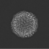
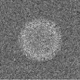
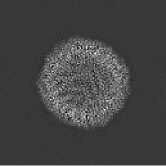
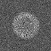
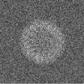
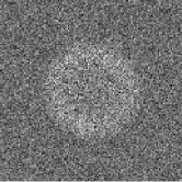
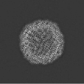
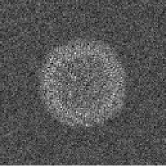
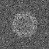
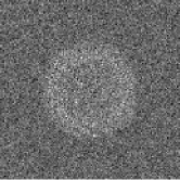
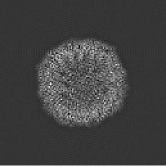
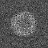
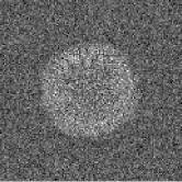
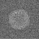
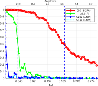
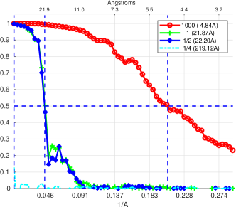
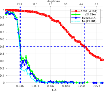
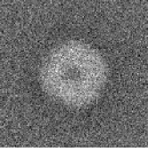
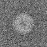
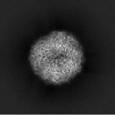
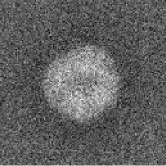
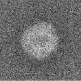
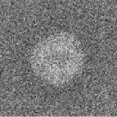
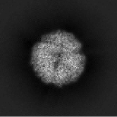
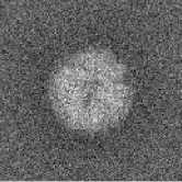
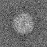
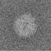
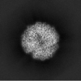
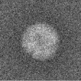
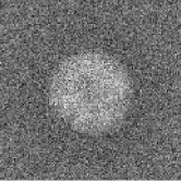
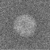
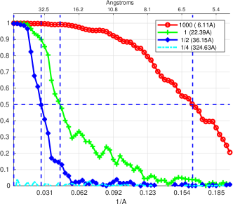
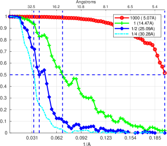
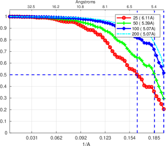
To test the performance of our algorithm in the presence of noise, we applied it to noisy simulated projection-images as follows. For symmetry, we downloaded from EMDB the map EMD-4905 [10], generated from it clean projection-images of size pixels, and added to the clean images Gaussian noise with zero mean and variance that results in signal to noise ratio (SNR) of the images the is equal to 1000 (considered as clean images for reference), , , and (the signal to noise ratio is defined as the ratio between the energy of the signal in the image and the energy of the noise). Figure 2 shows several examples of projection-images of EMD-4905 at these noise levels.


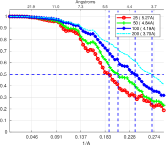
We then applied our algorithm on sets of images at these noise levels. For each group of images, we plot in Fig. 3 the Fourier shell correlation curve (FSC) [24] of the volume reconstructed by our algorithm relative to the ground truth volume. In a nutshell, the FSC measures the size of the smallest feature in the reconstructed volume that can be resolved. Figure 3 shows that increasing the number of input images improves the performance of the algorithm in terms of the achieved resolution. Moreover, we see that the algorithm fails for some of the noise levels (achieved resolution worse than 30 Å), but as we increase the number of images, the algorithm successfully reconstructs a three-dimensional model of the molecule, with resolution of about 20 Å. To further demonstrate this point, we show in Figure 4 the Fourier shell correlation curves for a fixed SNR and a variable number of images. As before, increasing the number of images improves the achieved resolution. The timing (in seconds) of the algorithm is summarized in Table 2. These timings were computed by averaging for each the timing results for all SNRs (as the running time is independent of the noise level).
| N | 25 | 50 | 100 | 200 |
| Time (sec) | 282 | 852 | 2,842 | 11,177 |
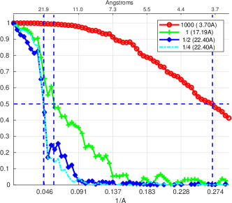
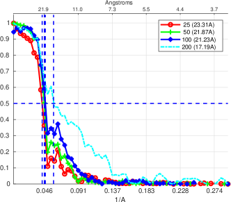
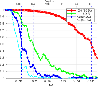
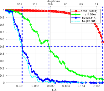
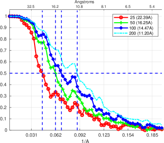
The results of the same experiment for symmetry with projections generated from EMD-10835 [14] are shown in Figs. 5, 6 and 7. The timing for symmetry is summarized in Table 3.
| N | 25 | 50 | 100 | 200 |
| Time (sec) | 397 | 1,352 | 5,178 | 20,228 |
5.2 Experimental data
Next, we applied our algorithm to two experimental data sets – EMPIAR-10272 and EMPIAR-10389 from the EMPIAR repository [8]. The EMPIAR-10272 data set corresponds to EMD-4905 [10] that has symmetry, and the EMPIAR-10389 data set corresponds to EMD-10835 [14] that has symmetry. For comparison, we also generated an ab-initio models from these data sets using Relion [26].
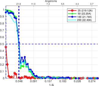
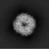
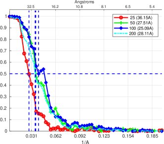
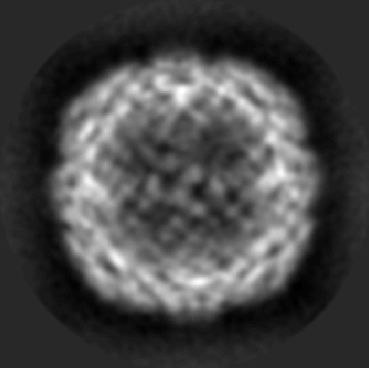
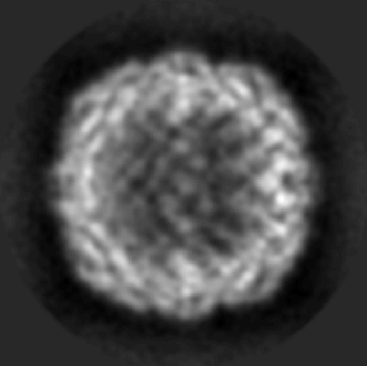
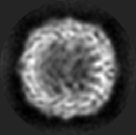
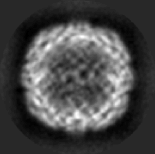
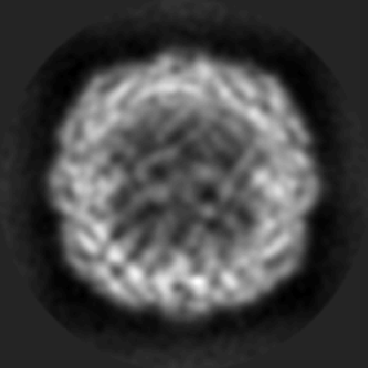
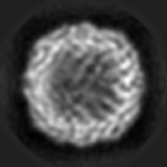
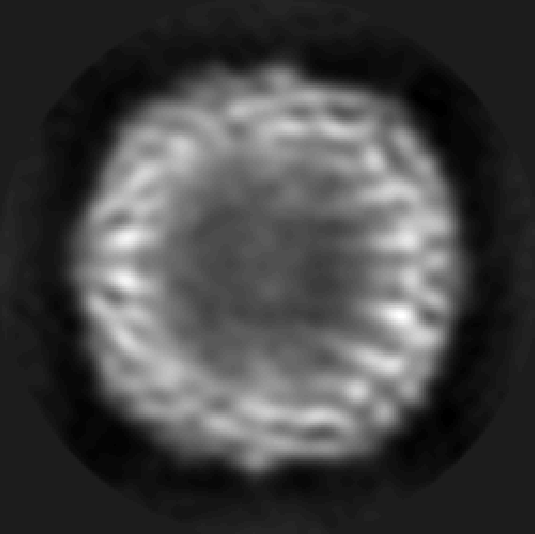
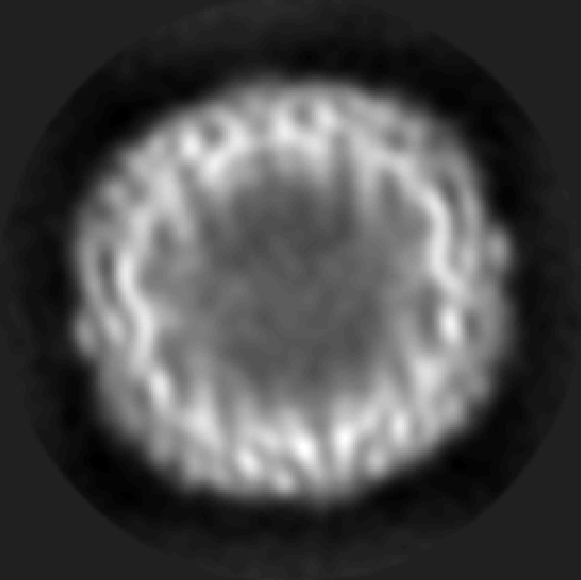
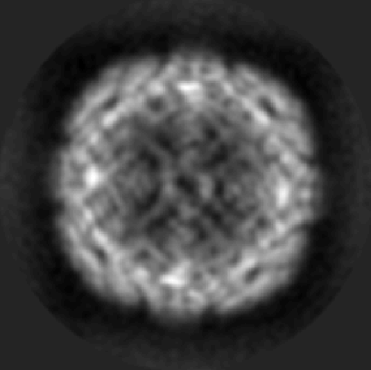
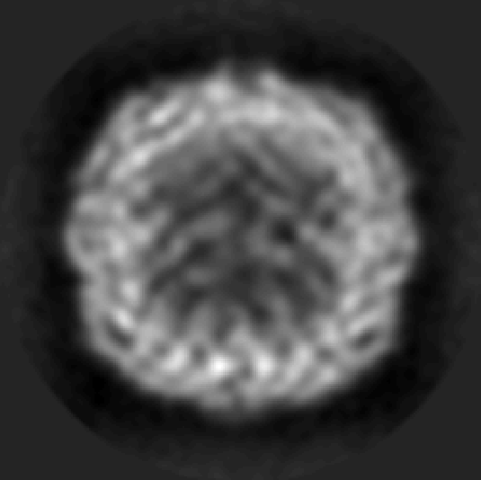
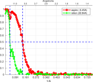
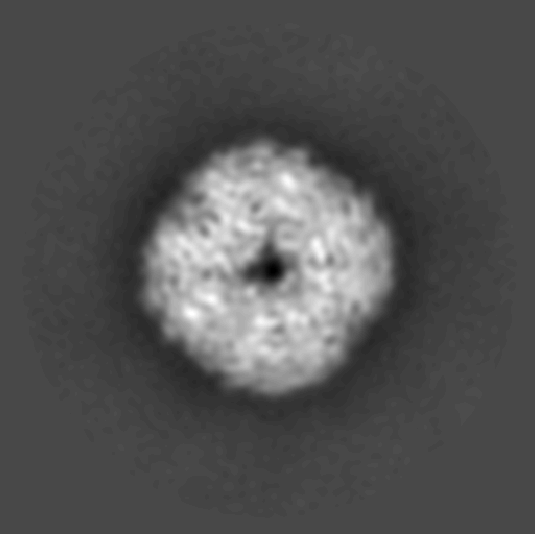
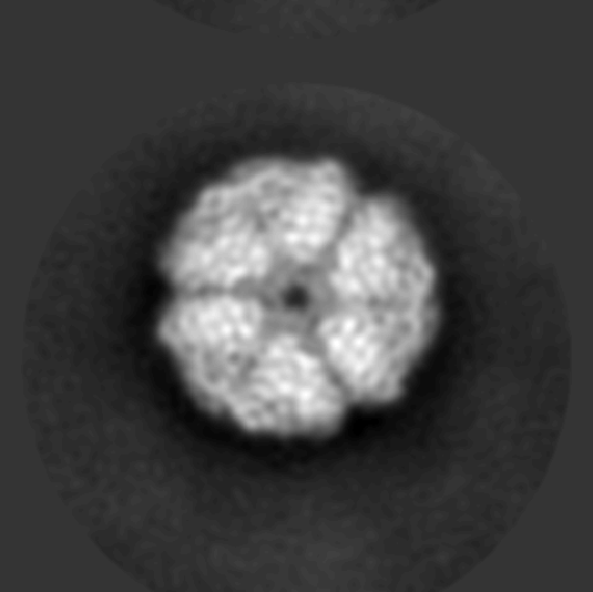
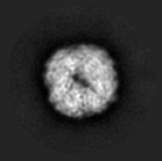
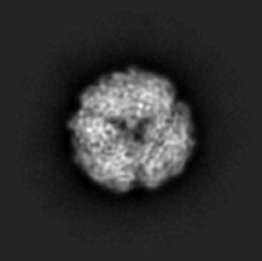
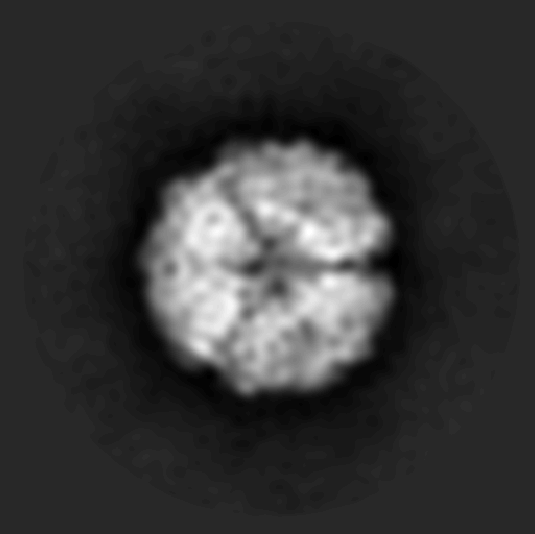
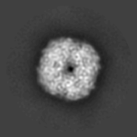
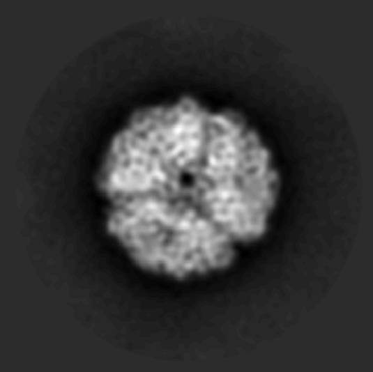
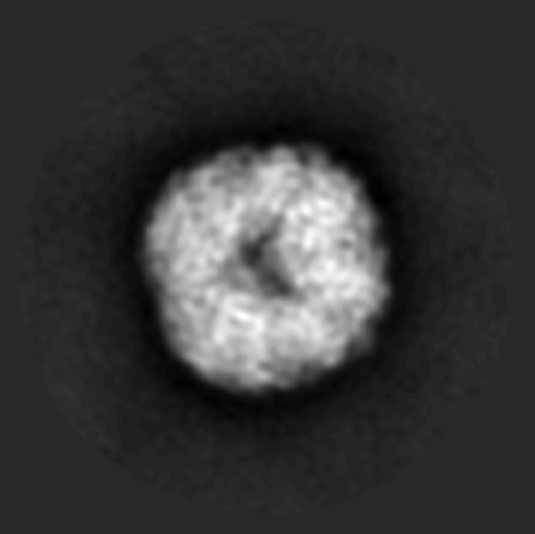
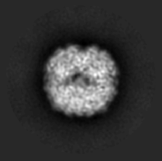
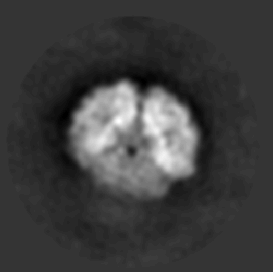
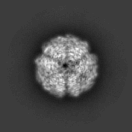
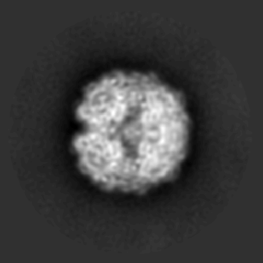
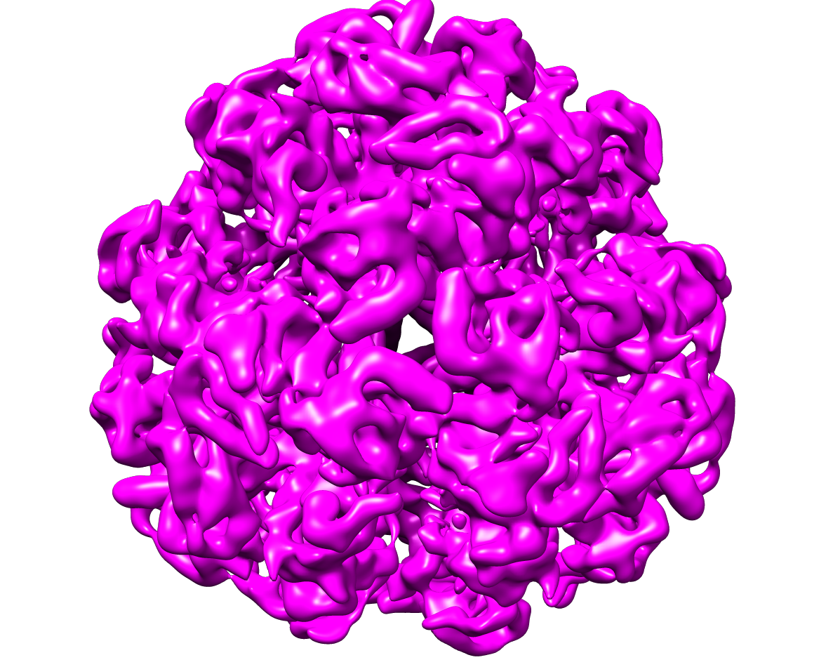
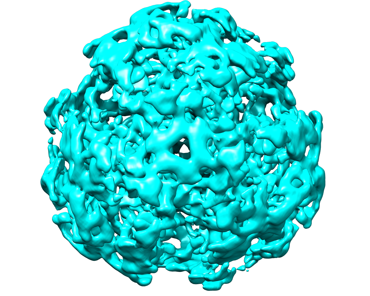
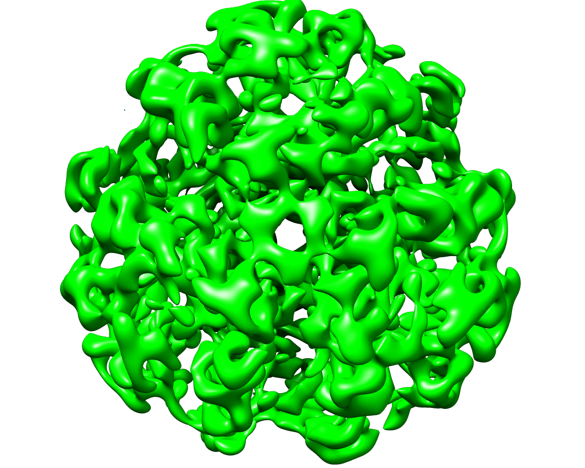
The EMPIAR-10272 data set consists of 480 micrographs, each comprised of 38 raw unaligned movie frames, with pixel size of 0.65 Å/pixel. We first applied motion correction to the movie frames using MotionCor2 [25], resulting in aligned micrographs, to which we applied CTF estimation [5] using CTFFind4 [15]. All subsequent processing steps were executed in Relion [26]. We used Laplacian auto-picking followed by one round of 2D classification to generate templates for template-based picking. Auto-picking resulted in 80,806 particles, which were subjected to 15 rounds of 2D classification, until 24,540 particles in 13 classes were retained. These 13 classes (Fig. 8) were the input to our algorithm, and resulted in an ab-initio model whose resolution is 6.45 Å (compared to the ground-truth density map EMD-4905 [10]). For comparison, we generated a three-dimensional ab-initio model using Relion, using as an input the same particles that were used to generate the class averages for our algorithm. The resolution of the model estimated by Relion 22.84 Å (also compared to the ground-truth density map EMD-4905 [10]). The Fourier shell correlation curves [24] for the initial models generated by our algorithm and by Relion are shown in Fig. 9. To assess visually the two models, we show in Fig. 10 a two-dimensional view of the ground-truth volume, the volume reconstructed by our algorithm (denoted ASPIRE in the figure), and the volume reconstructed by Relion. It can be observed that for this data set, the initial model generated by Relion is clearly inferior to the one generated by our algorithm.
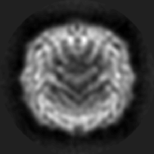
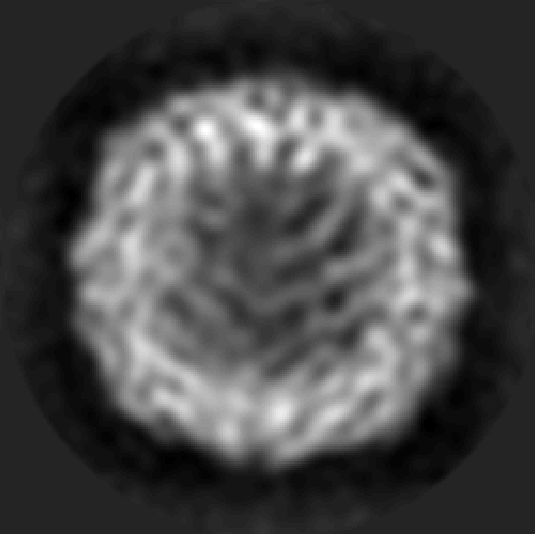
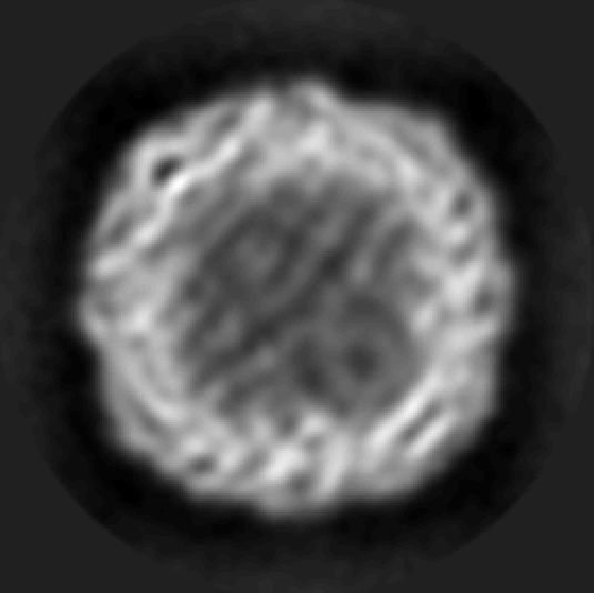
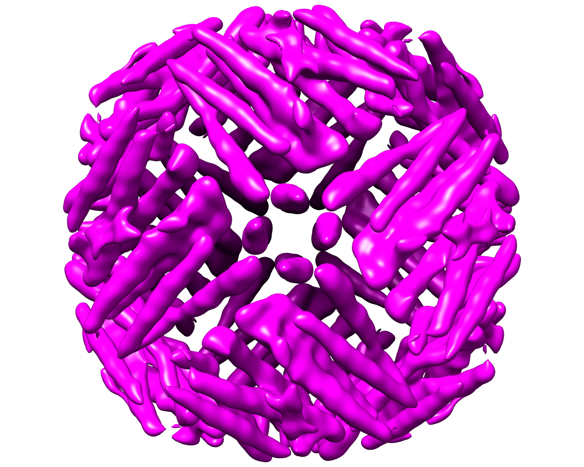
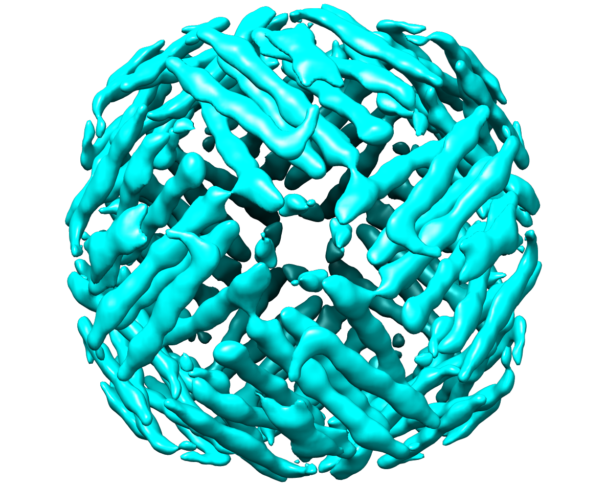
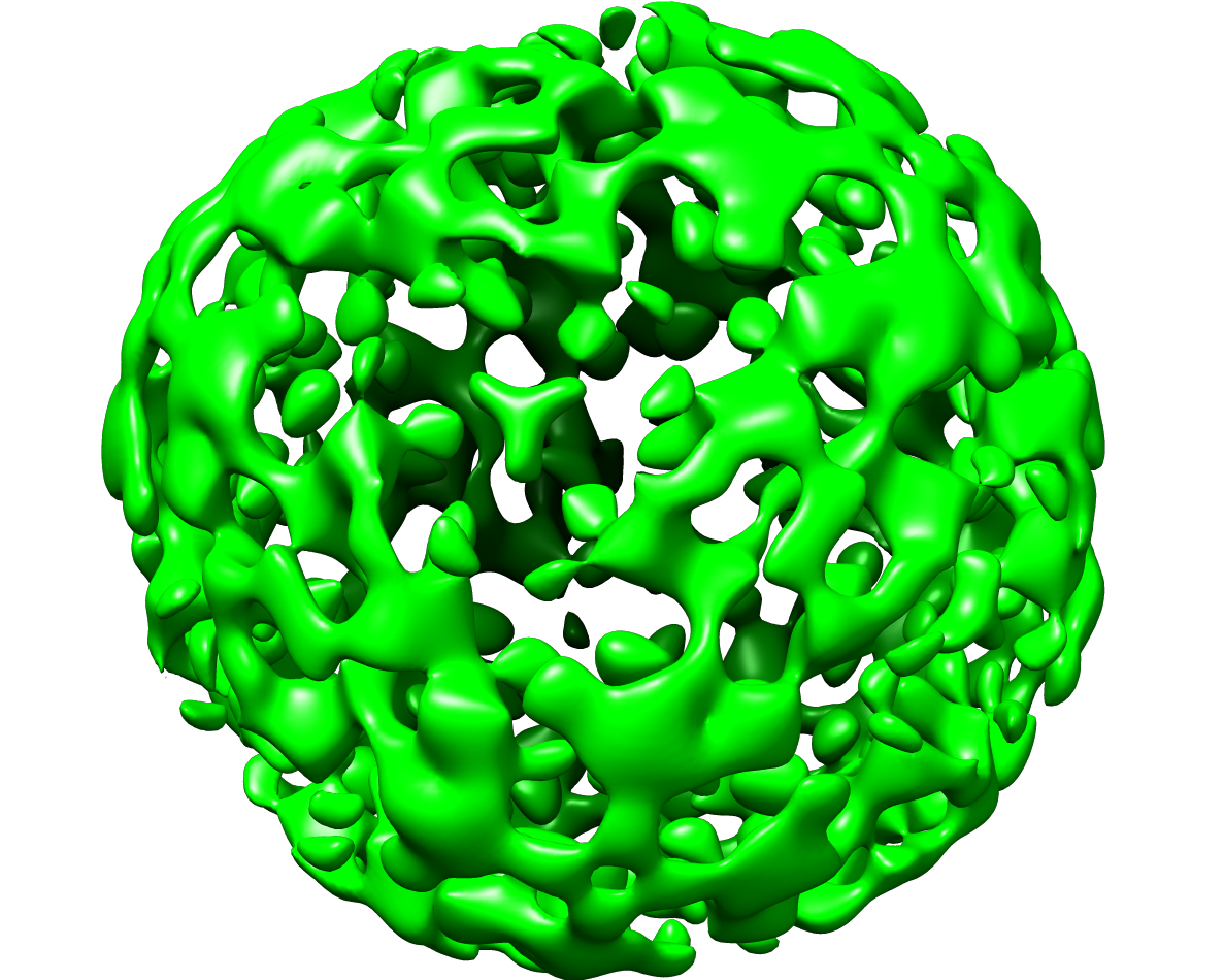
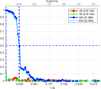
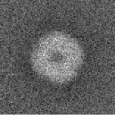
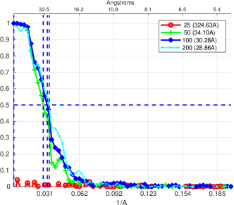
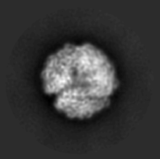
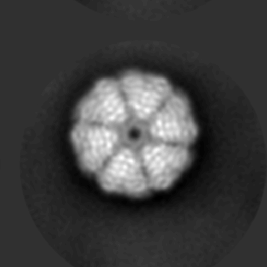
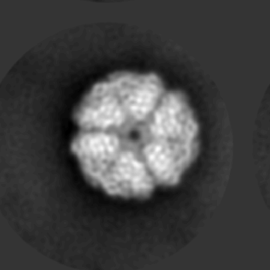
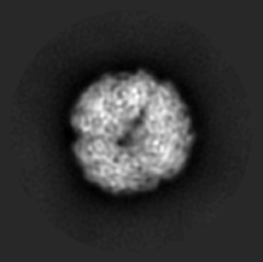
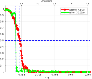
Next, we tested our algorithm on the EMPIAR-10389 data set, which has symmetry. The EMPIAR-10389 data set consists of 4,313 dose-weighted micrographs with pixel size of 0.639 Å/pixel. Automatic particle picking was done using the KLT picker [4], resulting in 164,183 particles of size 512 512 pixels. (We note that for the EMPIAR-10272 data set discussed above, we used Relion’s particle picker, as it gave superior results.) The particles were then imported into Relion [26], and were subjected to 5 rounds of 2D classification, until 63,057 particles remained in 30 classes. These classes were used as the input to our algorithm, and are shown in Fig. 11. The resolution of the resulting ab-initio model compared to the ground-truth density map EMD-10835 [14] is 7.31 Å. Using Relion’s initial model algorithm on the particles of these 30 classes resulted in a resolution of 10 Å (also compared to the ground-truth density map EMD-10835). The Fourier shell correlation curves for the initial models generated by our algorithm and by Relion are shown in Fig. 12. As before, we show in Fig. 13 two-dimensional views of the ground-truth volume EMD-10835, the volume reconstructed by our algorithm, and the volume reconstructed using Relion.
6 Future work
In this work, we proposed a method for estimating the orientations corresponding to a given set of projection-images of a molecule with tetrahedral or octahedral symmetry. The method relies on the observation that the elements of the tetrahedral and octahedral symmetry groups may be represented as rotation matrices with exactly one nonzero entry in each row and each column which is equal to either 1 or -1.
A future extension of this work would be to generalize it to molecules with icosahedral symmetry denoted by . Since the elements of the icosahedral symmetry group cannot be represented as rotation matrices with exactly one nonzero entry in each row and each column which is equal to either 1 or -1, the method suggested in this work is not applicable to this symmetry.
Acknowledgments
This research was supported by the European Research Council (ERC) under the European Union’s Horizon 2020 research and innovation programme (grant agreement 723991 - CRYOMATH) and by the NIH/NIGMS Award R01GM136780-01.
Appendix A Symmetry group elements
A.1 Tetrahedral group
| element | matrix | axis | angle | single-entry sum | one-line notation |
| any | 0 | ||||
| [1,1,1] | |||||
| [1,1,1] | |||||
| [-1,-1,1] | |||||
| [-1,-1,1] | |||||
| [1,-1,-1] | |||||
| [1,-1,-1] | |||||
| [-1,1,-1] | |||||
| [-1,1,-1] | |||||
| [1,0,0] | |||||
| [0,1,0] | |||||
| [0,0,1] |
A.2 Octahedral group
| element | matrix | axis | angle | single-entry sum | one-line notation |
| any | 0 | ||||
| [0,0,1] | |||||
| [0,0,1] | |||||
| [1,0,0] | |||||
| [1,0,0] | |||||
| [1,-1,1] | |||||
| [1,-1,1] | |||||
| [-1,1,1] | |||||
| [-1,1,1] | |||||
| [-1,-1,-1] | |||||
| [-1,-1,-1] | |||||
| [0,1,0] | |||||
| [0,1,0] | |||||
| [1,1,-1] | |||||
| [1,1,-1] | |||||
| [0,0,1] | |||||
| [0,1,-1] | |||||
| [1,0,0] | |||||
| [1,-1,0] | |||||
| [0,1,0] | |||||
| [1,1,0] | |||||
| [0,1,1] | |||||
| [1,0,1] | |||||
| [1,0,-1] |
Appendix B Proof of Lemma 7
Proof.
First, note that for the matrices and defined in Definition 4, it holds that
| (55) |
In addition, for any single entry matrix defined in Definition 4, it follows by a direct calculation that . By expressing and using Lemma 6, we have
For (36), we have that for
where the last equality follows by (55). For (37), we use (36) and obtain
For (38),
where the last equality follows by (55), and thus
Appendix C Constructing
We denote by the finite subset of rotations for the symmetry group on which we search for the optimum of the score function of (23). A naive choice for would be an almost equally spaced grid of rotations from , denoted as and defined below. However, the symmetry of allows us to significantly reduce the number of rotations in this naive set while maintaining the same accuracy of our algorithm. Note that for any and , it holds that , and so the set of local coordinates is equal to the set of local coordinates . Thus, keeping both and in is redundant. Consequently, our objective is to find all pairs of rotations for which there exists such that , and filter either or from . The resulting set would be .
Since is finite, an exact equality between and is unlikely. Therefore, the proximity between and is determined up to pre-defined thresholds, based on their representation using viewing direction and in-plane rotation (see [18]) as follows. The viewing directions of and are given by their third columns and , respectively. If and are two rotations with the same viewing direction, i.e., , then the rotation matrix is an in-plane rotation matrix which has the form
| (56) |
where is the in-plane rotation angle (see [18]). If , then , and so . Hence, we define two thresholds; the viewing direction threshold , and the in-plane rotation angle threshold . For the viewing direction threshold, we define along with the condition
| (57) |
Satisfying condition (57) implies that the rotations and have nearby viewing directions, and so it is reasonable to assume that the angle
| (58) |
approximates the in-plane rotation angle of (56). We therefore define along with the condition
| (59) |
Once both conditions (57) and (59) hold, the proximity between and is sufficient to remove either or from .
Of course, it is possible to replace the proximity measure we have used above with any other proximity measure. The advantage of the measure we use is its simple geometric interpretation, which allows to easily set and interpret its thresholds.
It remain to show how to construct the set , which is the input of the above pruning procedure. To that end, we let be a positive integer, and let denote Euler angles. We construct by sampling the Euler angles in equally spaced increments as follows. First, we sample at points. Then, for each , we sample at points. Finally, for each pair , we sample at points. For each on this grid, we compute a corresponding rotation matrix by
where
Appendix D and
Proof.
A classification of the closed subgroups of is given in [6], stating that every closed subgroup of is conjugate to one of , , , , , , , (the icosahedral symmetry), (the trivial group). Moreover, and are closed subgroups of . Since for topological groups the normalizer of a closed subgroup is closed (Lemma 10 below) and since is indeed a topological group, the normalizers of the closed subgroups and in , i.e. and , are also closed subgroups, thus conjugate to one of the closed subgroups of .
By definition of the normalizer, , which precludes , , , and from being the normalizers of or , since each has at most one symmetry axis of order larger than 2, while both and have more than one such axis. In addition, and are simple groups [21, 2], and so have no non-trivial normal subgroups. By definition of the normalizer, is a normal subgroup of . Thus, since and have no non-trivial normal subgroups, neither nor are normal subgroups of or , which precludes and from being the normalizers of or . Since is normal in [2], we have that and thus it must hold that and .
Lemma 10.
Suppose is a topological group. Then, the normalizer of a closed subgroup of
is a closed subgroup.
Proof.
Fix and define the map by . Since is a topological group, is continuous as the composition of multiplication and inversion maps. Thus, the preimage of the closed subgroup under , defined by , is closed. As any intersection of closed sets is closed, the intersection
is closed.
References
- [1] ASPIRE - algorithms for single particle reconstruction. http://spr.math.princeton.edu/.
- [2] M. Artin. Algebra. Pearson, 2nd edition, 2010.
- [3] J. M. de la Rosa-Trevín, J. Otón, R. Marabini, A. Zaldívar, J. Vargas, J. M. Carazo, and C. O. S Sorzano. Xmipp 3.0: an improved software suite for image processing in electron microscopy. Journal of structural biology, 184(2):321–328, 2013.
- [4] A. Eldar, B. Landa, and Y. Shkolnisky. KLT picker: Particle picking using data-driven optimal templates. Journal of structural biology, 210(2):107473, 2020.
- [5] Frank, J. Three-Dimensional Electron Microscopy of Macromolecular Assemblies: Visualization of Biological Molecules in Their Native State. Oxford, 2006.
- [6] M. Golubitsky, I. Stewart, and D. G. Schaeffer. Singularities and groups in bifurcation theory: Volume II, volume 69 of Applied Mathematical Sciences. Springer, 1988.
- [7] I. Greenberg and Y. Shkolnisky. Common lines modeling for reference free ab-initio reconstruction in cryo-EM. Journal of structural biology, 200(2):106–117, 2017.
- [8] A. Iudin, P. K. Korir, J. Salavert-Torres, G. J. Kleywegt, and A. Patwardhan. EMPIAR: a public archive for raw electron microscopy image data. Nature methods, 13(5):387–388, 2016.
- [9] F. Natterer. The Mathematics of Computerized Tomography. Classics in Applied Mathematics. SIAM, 2001.
- [10] K. Naydenova, M. J. Peet, and C. J. Russo. Multifunctional graphene supports for electron cryomicroscopy. Proceedings of the National Academy of Sciences of the United States of America, 116(24):11718–11724, June 2019.
- [11] G. Pragier, I. Greenberg, X. Cheng, and Y. Shkolnisky. A graph partitioning approach to simultaneous angular reconstitution. IEEE transactions on computational imaging, 2(3):323–334, 2016.
- [12] G. Pragier and Y. Shkolnisky. A common lines approach for ab initio modeling of cyclically symmetric molecules. Inverse Problems, 35, 2019.
- [13] A. Punjani, J. L. Rubinstein, D. J. Fleet, and M. A. Brubaker. cryoSPARC: algorithms for rapid unsupervised cryo-EM structure determination. Nature Methods, 14:290–296, 2017.
- [14] R. D. Righetto, L. Anton, R. Adaixo, R. P. Jakob, J. Zivanov, M.-A. Mahi, P. Ringler, T. Schwede, T. Maier, and H. Stahlberg. High-resolution cryo-em structure of urease from the pathogen yersinia enterocolitica. Nature communications, 11(1):5101, October 2020.
- [15] A. Rohou and N. Grigorieff. CTFFIND4: Fast and accurate defocus estimation from electron micrographs. Journal of Structural Biology, 192(2):216–221, 2015.
- [16] E. Rosen and Y. Shkolnisky. Common lines ab initio reconstruction of -symmetric molecules in cryo-electron microscopy. SIAM Journal on Imaging Sciences, 13(4):1898–1944, 2020.
- [17] Y. Shkolnisky and A. Singer. Viewing direction estimation in Cryo-EM using synchronization. SIAM Journal on Imaging Sciences, 5(3):1088–1110, 2012.
- [18] A. Singer. Viewing angle classification of cryo-electron microscopy images using eigenvectors. SIAM Journal on Imaging Sciences, pages 723–759, 2011.
- [19] A. Singer, R. R. Coifman, F. J. Sigworth, D. W. Chester, and Y. Shkolnisky. Detecting consistent common lines in cryo-EM by voting. Journal of Structural Biology, 169(3):312–322, 2010.
- [20] A. Singer and Y. Shkolnisky. Modeling Nanoscale Imaging in Electron Microscopy, chapter Center of Mass operators for CryoEM - Theory and implementation, pages 147–177. Nanostructure Science and Technology. Springer, New York, 2012.
- [21] J. StillWell. Naive Lie Theory. Undergraduate Texts in Mathematics. Springer, 2008.
- [22] G. Tang, L. Peng, P. R. Baldwin, D. S. Mann, W. Jiang, I. Rees, and S. J. Ludtke. EMAN2: an extensible image processing suite for electron microscopy. Journal of Structural Biology, 157(1):38–46, 2007.
- [23] M. Van Heel. Angular reconstitution: a posteriori assignment of projection directions for 3D reconstruction. Ultramicroscopy, 21(2):111–123, 1987.
- [24] M. Van Heel and M. Schatz. Fourier shell correlation threshold criteria. J. Struct. Biol., 151(3):250–262, 2005.
- [25] S. Zheng, E. Palovcak, J. P. Armache, K. Verba, Y. Cheng, and D. Agard. MotionCor2: anisotropic correction of beam-induced motion for improved cryo-electron microscopy. Nature methods, 14(4):331–332, 2017.
- [26] J. Zivanov, T. Nakane, B. O. Forsberg, D. Kimanius, W. J. Hagen, E. Lindahl, and S. H. Scheres. New tools for automated high-resolution cryo-EM structure determination in RELION-3. Elife, 7:e42166, 2018.