On the Influence of Enforcing Model Identifiability on Learning dynamics of Gaussian Mixture Models

Abstract

A common way to learn and analyze statistical models is to consider operations in the model parameter space. But what happens if we optimize in the parameter space and there is no one-to-one mapping between the parameter space and the underlying statistical model space? Such cases frequently occur for hierarchical models which include statistical mixtures or stochastic neural networks, and these models are said to be singular. Singular models reveal several important and well-studied problems in machine learning like the decrease in convergence speed of learning trajectories due to attractor behaviors. In this work, we propose a relative reparameterization technique of the parameter space, which yields a general method for extracting regular submodels from singular models. Our method enforces model identifiability during training and we study the learning dynamics for gradient descent and expectation maximization for Gaussian Mixture Models (GMMs) under relative parameterization, showing faster experimental convergence and a improved manifold shape of the dynamics around the singularity. Extending the analysis beyond GMMs, we furthermore analyze the Fisher information matrix under relative reparameterization and its influence on the generalization error, and show how the method can be applied to more complex models like deep neural networks.

1 Introduction

While a central focus of current research aims to understand the behavior of a model in the parameter space, for example, by studying optimizers and what local optima they converge to, most research does not include the interdependence of the parameters and the underlying probability space that the model lays in. This interdependence becomes especially interesting if the map from the parameter space to the probability distribution is not one-to-one resulting in the Fisher Information Matrix (FIM) to not being positive definite but only positive semi-definite [Wat09]. In information science such a parametric model is called singular. More formally, a model $\{m_{\theta}(x)\ :\theta\in\Theta\}$ is said to be identifiable iff the mapping $\theta\mapsto m_{\theta}(x)$ is one-to-one. Furthermore a model is said regular if it is both identifiable and $\partial_{1}m_{\theta}(x),\ldots,\partial_{D}m_{\theta}(x)$ are linearly independent. A regular model allows to define a manifold with tangent planes at $m_{\theta}$ using the basis $\{\partial_{i}m_{\theta}(x)\}$. In the vanilla case, a parametric statistical model is regular and identifiable, but even very simple examples violate this assumption. Consider, for example, a gaussian model is regular but a mixture model thereof is not identifiable. An exponential family with non-minimal sufficient statistics is not regular (the tangent vectors $\partial_{i}m_{\theta}(x)$ are not linearly independent).

The study of singular models is a very relevant setting in practice as a lot of statistical models used in practice, such as artificial neural networks [VDM86], reduced rank regressions [VRW86], normal or binomial mixtures, hidden Markov models [BP66], stochastic context-free grammars [Cho56, ED94] and Bayesian networks are singular models. For all those singular models, we consider two main problems: firstly one can easily observe that all standard information criteria (see e.g. Bayesian information criterion (BAC) [Sch78] or Akaike information criterion (AIC)[Aka74]) do no longer hold in this setting. Secondly it can be observed that singular points in the parameter space induce attractor behavior of the learning trajectories [Wei+08, Ama+18, APO06].

In this paper we introduce and analyze the idea of enforcing model identifiability during training by relative reparameterization to improve the behaviour of the learning dynamics near the singularities. The fundamental idea of the proposed reparameterization is to fix a arbitrary reference parameter and define all other parameters relative to it. While the idea of parameter ordering is used during the theoretical analysis of singular model the important difference is that we consider the influence of enforcing this setting also during training on the learning dynamics. As illustrated in Eq. 1 this allows us to construct a new parameter space that has a bijection to the model probability space.

Contributions. (1) We introduce a relative reparameterization of the parameter space that presents a general way to extract identifiable models from singular ones. (2) For Gaussian mixture models (GMMs) with two components, we illustrate the change of expected gradient decent dynamics around the singularity under reparameterization as well as the a new version of Expectation Conditional Maximization (ECM) algorithm for the reparameterized setting. (3) Finally building a foundation for a deeper future analysis we show first theoretical properties related to the Fisher information and generalization error from a learning theoretical perspective, and illustrate how relative reparameterization can easily be applied to more complex models like neural networks.

2 Singular Models and Relative Reparameterization

We start with formalizing the above notion of singularities and relative reparameterization. Let a parametric regular statistical model $\mathcal{P}$ be a family of probability distributions $\mathcal{P}=\{p_{\theta}\ :\ \theta\in\bm{\Theta}\}$ where $p_{\theta}$ is a function parameterized by $\theta$, an open subset of $\mathbb{R}^{K}$. A statistical model is said identifiable iff

$$p_{\theta}=p_{\theta^{\prime}}\quad\Leftrightarrow\quad\theta=\theta^{\prime}.$$

Consider two functions $f(\bm{X}|\bm{\Phi})$ and $g(\bm{X}|\bm{\Theta},\bm{\Phi})$ parameterized by $\bm{\Theta}=\{\theta_{1},\cdots,\theta_{K}\}$ and $\bm{\Phi}=\{\phi_{1},\cdots\phi_{M}\}$ and let $\bm{X}=\{\bm{x}_{1}^{\top},\cdots,\bm{x}_{N}^{\top}\},~{}{\bm{x}}_{i}^{\top}\in{\mathbb{R}}^{D}$ be the input data. While there is a variety of constructions that can induce singularities (see e.g. [Wat09]) the two main cases that lead to a model being not identifiable are:

1. Elimination singularity: considers the following relation between $g(\cdot)$ and $f(\cdot)$, $g(\bm{X}|\theta_{1},\bm{\Phi}):=\theta_{1}f(\bm{X}|\bm{\Phi})$ where we see that the parameter $\bm{\Phi}$ is no longer identifiable if $\theta_{1}=0$. Informally if a function is multiplied with zero the parameters of this function can not be identified. Further note that elimination singularity is a kind of avoiding model selection (in mixtures when some weights are zero).

2. Overlap singularity considers a setting where $g(\cdot)$ is defined as a weighted sum of $f(\cdot)$ such that $g(\bm{X}|\bm{\Theta},\bm{\Phi}):=\sum_{k=1}^{K}\theta_{k}f(\bm{X}|\phi_{k})$. One can observe that if $\theta_{i}=\theta_{j}$ we cannot identify the parameters $\phi_{i},\phi_{j}$. This gets clear by considering $g(\bm{X}|\Theta,\Phi)=\theta_{i}f(\bm{X}|\phi_{i})+\theta_{j}f(\bm{X}|\phi_{j})+\sum_{k\neq i,j}\theta_{k}f(\bm{X}|\phi_{k})$. Informally this means that if we consider a linear combination of functions and the combination weights coincide then the parameters of the functions become unidentifiable.

Both of the settings can be found for example, in mixture models or neural networks. We can now construct a reparameterization of the parameter space that allows us to avoid the above singularities by defining it in terms of a quotient space [AMS08, Wil70]. Let $\bm{\Theta}$ be a parameter space equipped with an equivalence relation $\sim$, such that reflexivity, symmetry and transitivity hold. Given some parameter $\theta_{i}$, $[\theta_{i}]:=\{\theta_{j}\in\bm{\Theta}:\theta_{i}\sim\theta_{j}\}$ gives the parameters, that map to the same distribution. Furthermore $\bm{\Theta}/\sim:=\{[\theta_{i}]:\theta_{i}\in\bm{\Theta}\}$ gives the set of all parmeterizations for statistical models that can be modeled by $\theta_{i}\in\bm{\Theta}$. Now we use $\xi(\theta)$ to denote $[\theta]$, which is a point on the quotient and $[\theta]=\xi^{-1}(\xi(\theta))$ as a subset of $\bm{\Theta}$. Clearly $\xi(\theta)=\xi(\theta^{\prime})$ iff $\theta\sim\theta^{\prime}$. A function $p$ on $\bm{\Theta}$ is invariant under $\sim$ if $p_{\theta}=p_{\theta^{\prime}}$ whenever $\theta\sim\theta^{\prime}$ in which case the function $p$ induces a unique function $\overline{p}$ on, where $\bm{\Theta}/\sim$ is the projection on $p$ s.t. $p:=\overline{p}\circ\xi$

(1)

The smoothness of $\overline{p}$ can be checked by $\bm{\Theta}/\sim$ being a quotient manifold, and let $\overline{p}$ be a function on $\bm{\Theta}/\sim$. Then $\overline{p}$ is smooth iff $p:=\overline{p}\circ\xi$ is a smooth function on ${\mathcal{P}}$. To ensure that there are no parameters in an equivalence relation we impose the following constraint:

$$\forall i,j\in\{1,\cdots,K\},i\neq j~{}\exists l:~{}|\bm{\theta}_{i}^{l}-\bm{\theta}_{r}^{l}|\not=|\bm{\theta}_{j}^{l}-\bm{\theta}_{r}^{l}|$$

where we set $\bm{\theta}_{r}^{l}$ to be a reference parameter used to construct an ordering. In the high dimensional case we denote the $l$-th component of $\bm{\theta}_{i}$ as $\bm{\theta}_{i}^{l}$. Referring back to the probability space we can now use this parameter subspace to define an identifiable submodel. Now let $\mathcal{P}=\{p_{\theta}\ :\ \theta\in\bm{\Theta}\}$, then a submodel as $\mathcal{S}\subset\mathcal{P}$ can be defined over a subset of the parameterspace: $\mathcal{S}=\{p_{\theta}^{\prime}\ :\ \theta^{\prime}\in\bm{\Lambda}|\bm{\Lambda}\subseteq\bm{\Theta}\}$. Having defined the properties of the new parameter space we can now define a procedure to construct such a space from the original parameter space.

Relative Reparameterization. Consider an overlap singularity where we can not identify $\bm{\phi}_{i},\bm{\phi}_{j}$ iff $\bm{\theta}_{i}=\bm{\theta}_{j}$. Now starting from a parameterization $\bm{\Theta}=\left\{\bm{\theta}_{1},\cdots\bm{\theta}_{K}\right\}$ and want to ensure an ordering of the form $\exists l\quad\bm{\theta}_{\sigma(1)}^{l}<\bm{\theta}_{\sigma(2)}^{l}<\cdots<\bm{\theta}_{\sigma(K)}^{l}$ where $\sigma(\cdot)$ is a permutation that describes the parameter ordering after initialization. Wlog. let $\bm{\theta}_{\sigma(1)}$ be the reference parameter. To enforce this define a set of relative parameters over the difference $\{\Delta_{i}\}_{i=1}^{K-1}$ such that for any consecutive two parameters with $k\in\{2,\cdots,K\}$

$$\xi:\exists l\quad\bm{\theta}^{l}_{\sigma(k)}\stackrel{{\scriptstyle\text{rep.}}}{{\longrightarrow}}\bm{\theta}^{l}_{\sigma(k-1)}+\Delta_{k-1}\qquad\Rightarrow\qquad\exists l\quad\bm{\theta}_{\sigma(1)}^{l}\leq\bm{\theta}_{\sigma(2)}^{l}\leq\cdots\leq\bm{\theta}_{\sigma(K)}^{l}$$

holds and therefore the set of parameters changes from $\bm{\Theta}:=\left\{\bm{\theta}_{1},\cdots\bm{\theta}_{K}\right\}$ to $\bm{\Lambda}:=\left\{\bm{\theta}_{1},\Delta_{1}\cdots\Delta_{K-1}\right\}$. To preserve the ordering during optimization we have to ensure that $\Delta_{i}>0$. We can consider two ways to approach this:

1. Use constraint optimization with $\Delta_{i}>0$.

2. Optimize on $\Delta_{i}^{2}$ instead of $\Delta_{i}$, ensuring $\Delta_{i}\geq 0$ and add a clearance threshold $\xi>0$ such that $\Delta_{i}+\xi>0$.

Clearance Threshold. We can now extend the above to further address elimination singularities by adding a clearance threshold:

$$g(\bm{X}|\bm{\theta}_{1},\bm{\Phi},\lambda)=(\bm{\theta}_{1}+\lambda)f(\bm{X}|\bm{\Phi}),\quad\lambda\in{\mathbb{R}}_{+}$$

Therefore $\lambda$ changes how close the parameters can be to the singularity, which is now given by $\Delta=0$ instead of $\bm{\theta}_{i}=\bm{\theta}_{j}$ in the initial parameterization. Note that for the extend of this paper we focus on the influence of relative reparameterization and treat $\lambda$ as a hyperparameter for defining strong identifiability and therefore not include it in the set of parameters that are optimized. Thus by varying $\lambda$, we can get a filtration of regular models an in the limit $\lambda=0$ the singular model.

3 Dynamics of Gradient Descent Learning under Reparameterization

To illustrate the influence of the above introduced reparmeterization we look at the well established problem of learning Gaussian mixtures. Considering a normal distribution $\mathcal{N}\left(\bm{X}|\mu_{k},\sigma_{k}\right)$ parameterized by the mean $\mu_{k}$ and standard deviation $\sigma_{k}$. Then the mixture of $K$ components $p\left(\bm{X}|\left\{\bm{\pi}_{k},\bm{\mu}_{k},\bm{\sigma}_{k}\right\}_{K}\right)=\sum_{k=1}^{K}\pi_{k}\mathcal{N}\left(\bm{X}|\mu_{k},\sigma_{k}\right)$ under the constraint that the mixture components, $\{\pi_{k}\}$ lay on the probability simplex, such that $\sum_{k=1}^{K}\pi_{k}=1\text{ and }\pi_{k}\geq 0\quad\forall k\in\{1,\cdots K\}$ [BV04]. Given data sampled from the mixture the goal is now to recover the parameters $(\left\{\bm{\pi}_{k},\bm{\mu}_{k},\bm{\sigma}_{k}\right\}_{K})$.

3.1 Dynamics around Singularity

Singularities and Reparameterization. For easier analysis and illustration consider the specific case of $K=2$ (arguments directly extend to higher dimensions as well) such that the $2$-GMM is given by: $p(\bm{X}|\bm{\Theta})=\pi_{1}\mathcal{N}\left(\bm{X}|\mu_{1},\sigma_{1}\right)+(1-\pi_{1})\mathcal{N}\left(\bm{X}|\mu_{2},\sigma_{2}\right).$ We can now describe the singularities as defined in Section 2 with respect to the different components. (1) Mixture component: If we consider $\pi_{1}=\{0,1\}$, since $\pi_{2}=1-\pi_{1}$ we get $\pi_{2}=\{1,0\}$, and can no longer identify the parameters $\{\mu_{1},\mu_{2}\}$ as well as $\{\sigma_{1},\sigma_{2}\}$. (2) Mean: if we consider $\mu_{1}=\mu_{2}$ the parameter for the mixture, $\{\pi_{1},\pi_{2}\}$ and $\sigma_{1}=\sigma_{2}$ are unidentifiable. (3) Standard deviation: similarly if we consider $\sigma_{1}=\sigma_{2}$ for the standard deviation the parameter for the mixture, $\{\pi_{1},\pi_{2}\}$ and $\mu_{1}=\mu_{2}$ are unidentifiable.

From there we define the relative reparemeterization as $\bm{\Theta}=\{\mu_{1},\mu_{2},\sigma_{1},\sigma_{2},\pi_{1}\}\stackrel{{\scriptstyle\text{rep.}}}{{\longrightarrow}}$ $\{\mu_{1},\Delta_{\mu},\sigma_{1},$ $\Delta_{\sigma},\pi_{1}\}=\bm{\Lambda}$ which give an ordering for $\mu_{2}=\mu_{1}+\Delta_{\mu}\Rightarrow\mu_{1}<\mu_{2}$ and $\sigma_{2}=\sigma_{1}+\Delta_{\sigma}\Rightarrow\sigma_{1}<\sigma_{2}$ where $\Delta_{\mu},\Delta_{\sigma}>0$. Note that while this provides the full reparameterization we focus on fixing all but one parameter in the following and only look at the singularity with respect to this parameter.

Learning Dynamics. To analyze the model we can now consider the setting of learning the parameters with a gradient decent by minimizing the following objective function: ${L}_{\Theta}({\bm{X}})=\frac{1}{n}\sum_{i=1}^{n}l(x;\theta)$ where $l(x;\theta)$ is the log likelihood. Then the standard GD update is defined as $\theta_{t+1}=\theta_{t}+\eta\nabla L_{\Theta}({\bm{X}})$. For the analysis of the dynamics around the singularity we consider the general approach by [PO09] and extend it to the reparameterized setting. See supplementary material for further details and derivations. For this analysis consider two Gaussian components with unit variance and we furthermore define:

$$u =\mu_{1}-\mu_{2}\qquad u^{\prime} =\Delta$$

$$w =\pi\mu_{1}+(1-\pi)\mu_{2}\qquad w^{\prime} =\pi\mu_{1}+(1-\pi)(\mu_{1}+\Delta)$$

For the following analysis we assume that the number of data $N$ is sufficiently large and hence we use the expectation with respect to the true distribution $L(\theta)=\mathbb{E}\left[l(x;\theta)\right]$ we can obtain the average learning equation as the form of differential equations by assuming $\eta\rightarrow 0$ such that $\frac{\mathrm{d}\theta}{\mathrm{d}t}=\eta\nabla L(\theta)=\eta\ \mathbb{E}\left[\frac{\partial l}{\partial\theta}\right]$ and we analyze the dynamics of the simple Gaussian mixture model using the average learning equations, which is given by

$$\begin{aligned} \frac{\mathrm{d}v}{\mathrm{~{}d}t}&=\eta\mathbb{E}\left[\frac{\partial l}{\partial v}\right]\quad\text{and}\quad\frac{\mathrm{d}\mu_{i}}{\mathrm{~{}d}t}&=\eta\mathbb{E}\left[\frac{\partial l}{\partial\mu_{i}}\right]\ \forall i\in[K].\end{aligned}$$ (2)

Using a change of variables we can derive the averaged learning equations for the new parameters as $\mathbb{E}\left[\frac{\mathrm{d}v}{\mathrm{~{}d}t}\right],\mathbb{E}\left[\frac{\mathrm{d}u}{\mathrm{~{}d}t}\right]$ and $\mathbb{E}\left[\frac{\mathrm{d}w}{\mathrm{~{}d}t}\right]$, and similarly for the reparameterization as given in Eq. 2. As the exact expressions of the expectations blow up and do not give direct insight into the comparison of the dynamics we deffer it to the appendix. While the dynamics can be shown to slow down close to the singularity [PO09] an analytical comparison to the reparameterization is difficult. To better show this difference we consider the visualization in Figure 1 where we plot the dynamics in the $\mu_{1},\mu_{2}$ space while fixing $\pi=0.5$ and wlog. assume $\eta=1$. Here Figure 1 tow two rows, shows the dynamics around zero and we can observe that by considering relative reparmeterization (1) the magnitude of the gradients increase which indicates faster convergence with appropriate learning rates and more importantly (2) the reparameterization reduced valleys that can form in the landscape (see Figure 1, bottom two rows, middle column).

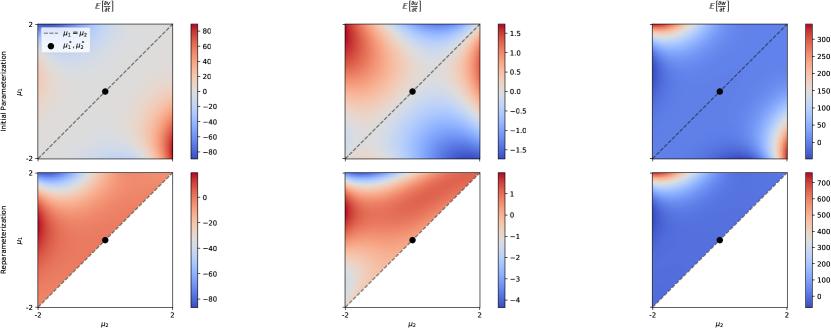
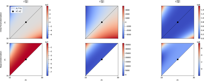
Figure 1: Average learning dynamics for initial and re-parameterization. For each plot the top row shows the dynamics for the initial parameterization plotted in the $\mu_{1},\mu_{2}$ space and the bottom row the dynamics for the reparameterization. (top two rows) $\mu_{1},\mu_{2}\in\{-2,2\}$ and $\{\mu_{1}^{*},\mu_{2}^{*}\}=\{0,0\}$ (bottom two rows)$\mu_{1},\mu_{2}\in\{10,30\}$ and $\{\mu_{1}^{*},\mu_{2}^{*}\}=\{20,20\}$.

4 Dynamics of Expectation Maximisation (EM)

After analyzing the learning dynamics under gradient decent we can now extend our analysis to EM algorithms. We start with a short recap of the standard EM for GMMs and then derive the update steps for under reparameterization for $2$-GMMs.

4.1 Expectation Maximisation Setup

The EM algorithm [New86, DLR77] has been applied widely on the maximum likelihood problem in mixture models as it has provable convergence to a critical point [Wu83]. The goal is to maximise the log likelihood $\ln\mathcal{L}(\bm{\Theta};\bm{X})$, which in the case of a GMM we can define as: $\ln p(\bm{X}|\bm{\pi},\bm{\mu},\bm{\Sigma})=\sum^{N}_{n=1}\ln\sum_{k=1}^{K}\pi_{k}\mathcal{N}(\bm{x}|\bm{\mu}_{k},\bm{\Sigma}_{k})$. We can find a local minima by iterative algorithms which consists of two steps: first calculate the expectation of the posterior $\gamma(z_{k})$ and then maximize for the parameters $\bm{\pi},\bm{\mu},\bm{\Sigma}$. We can formulate both steps as follows.

E-Step. Define $Q\left(\bm{\Theta}|\bm{\Theta}^{(t)}\right)$ as the expected value of the likelihood function of $\bm{\Theta}$, with respect to the current conditional distribution of $\bm{Z}$ given $\bm{X}$ and the current parameter estimate $\bm{\Theta}^{(t)}$ for time-step $t$: $Q\big{(}\bm{\theta}|\bm{\theta}^{(t)}\big{)}=\mathbb{E}_{\mathbf{Z}|\mathbf{X},\bm{\theta}^{(t)}}\left[\ln\mathcal{L}(\bm{\theta};\mathbf{X},\mathbf{Z})\right].$

M-Step. After we calculate the soft class assignment we want to find the parameters that maximize: $\bm{\theta}^{(t+1)}={\arg\max}_{\bm{\theta}}\quad Q\big{(}\bm{\theta}|\bm{\theta}^{(t)}\big{)}.$ Defining $N_{k}:=\frac{1}{N}\sum_{n=1}^{N}\gamma\left(z_{nk}\right)$, this give us the update for the mean as: $\bm{\mu}_{k}=\frac{1}{N_{k}}\sum_{n=1}^{N}\gamma\left(z_{nk}\right)\bm{x}_{n}$, for the $\pi_{k}=\frac{N_{k}}{N}$ for the mixture component and for covariance matrix $\mathbf{\Sigma}_{k}=\frac{1}{N_{k}}\sum_{n=1}^{N}\gamma\left(z_{nk}\right)\left(\bm{x}_{n}-\bm{\mu}_{k}\right)\left(\bm{x}_{n}-\bm{\mu}_{k}\right)^{\top}$.

4.2 EM for Reparamterization $\mu_{1},\mu_{2}\stackrel{{\scriptstyle\text{rep.}}}{{\longrightarrow}}\mu_{1},\Delta$

For simplicity of analysis and to be able to plot the learning trajectories and visualize the parameter space for the 2-GMM we fix $\bm{\pi}=0.5,\sigma_{1}=1,\sigma_{2}=1$ and optimize $\mu_{1},\mu_{2}$. Therefore the 2-GMM simplifies to $p(\bm{X}|\mu_{1},\mu_{2})=0.5\mathcal{N}\left(\bm{X}|\mu_{1},1\right)+0.5\mathcal{N}\left(\bm{X}|\mu_{2},1\right)$.

Now this model only considers learning the means, $\mu_{1},\mu_{2}$ and we note that the other parameters of the model are not identifiable — we can not identify if the value for a variance can be attributed to the first or second mixture component — in the case of $\mu_{1}=\mu_{2}$. To avoid this we consider the reparameterisation $\{\mu_{1},\mu_{2}\}\stackrel{{\scriptstyle\text{rep.}}}{{\longrightarrow}}\{\mu_{1},\Delta\}$.

Starting from the above definitions of the EM algorithm we have to consider a slight change in the update rule as $\Delta$ is part of the update rule for $\mu_{1}$ and vice versa. Therefore we consider Expectation Conditional Maximization (ECM) [MR93]. Here, while the E-Step stays the same, the M-step is replaced with a sequence of conditional maximization (CM). Here each parameter is maximized individually, conditionally on the other parameters remaining fixed. We can explicitly write out the updates as shown in Algorithm 2 for the specific $2$-GMM case introduce above.

Algorithm 1 Relative Reparamterization Expectation Conditional Maximization

1:Define log likelihood: $\ln p(\bm{X}|\pi,\bm{\mu},\bm{\sigma})=\sum^{N}_{n=1}\ln\sum_{k=1}^{2}\pi_{k}\mathcal{N}(\bm{x}|\bm{\mu}_{k},\bm{\sigma}_{k})$

2:Define $\{\mu_{1},\mu_{2}\}\stackrel{{\scriptstyle\text{rep.}}}{{\longrightarrow}}\{\mu_{1},\Delta\}$

3:Fix $\sigma,\pi$

4:while $\left\lVert\ln\mathcal{L}(\bm{\Theta}^{(t-1)};\bm{X})-\ln\mathcal{L}(\bm{\Theta}^{(t)};\bm{X})\right\rVert>\varepsilon$ do

5:     E-Step. Compute: $Q\big{(}\bm{\theta}|\bm{\theta}^{(t)}\big{)}=\mathbb{E}_{\mathbf{Z}|\mathbf{X},\bm{\theta}^{(t)}}\left[\ln p(\bm{X}|\pi,\bm{\mu},\bm{\sigma})\right].$

6:     M-Step. Reference mean: $\mu_{1}=\frac{\sum^{N}_{n}z_{n1}\bm{x}_{n}\Delta\sum^{N}_{n}z_{n1}+\sum^{N}_{n}z_{n2}\bm{x}_{n}}{\sum^{N}_{n}z_{n1}+\sum^{N}_{n}z_{n2}}$

7:     M-Step. Relative Parameter: $\Delta=\frac{\sum^{N}_{n}z_{n2}\bm{x}_{n}-\mu_{1}\sum^{N}_{n}z_{n2}}{\sum^{N}_{n}z_{n2}}$

8:end while

We now illustrate the influence of the new update rule by plotting learning dynamics. Consider the following setup: we set the true parameters, $\bm{\Theta}^{*}$, of the data to be near the singularity, which means that $\mu_{1}\approx\mu_{2}$. We then initialize $\mu_{1},\mu_{2}$ away from the singularity and observe the learning trajectory in ${\mathbb{R}}^{2}$ in the initial and reparameterized parameter space. As shown in Figure 2, we can see the attractor-like behavior of the initial parameterization plotted in red when the parameters get closer to the singularity. This behavior can not be observed when looking at the learning trajectory for the relative reparameterization, plotted in blue. Both parameterizations have fast convergence of the log-likelihood, while the distance of the parameters to the true parameterization decrease faster for the relative reparameterization (Figure 2).

We can now note that this change in behavior is in line with the change of the gradients under reparameterization as shown in Figure 1

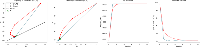
Figure 2: a) learning trajectory in the original coordinate system $\{\mu_{1},\mu_{2}\}$. Plotted is the trajectory under the original parameterization in red and for the reparameterization in blue. The true parameterization of the data is marked by a green cross. Furthermore the singularity, $\mu_{1}=\mu_{2}$ is shown by the dotted black line. b) Same setting as in the left plot but now the learning trajectories are plotted in the $\{\mu_{1},\Delta\}$ coordinate system. c) log likelihood for both parameterizations, d) euclidean distance between current and optimal parameterization

5 Properties of the Reparameterization

In previous sections we discussed the convergence properties under reparameterization and saw changes in the general landscape of the update gradients. While this paper provides an initial analysis of the idea and findings on convergence we now probe into further directions of analysis. As a central quantity in information geometry we first illustrate aspects of the FIM under reparameterization and then looking into the direction of classical learning theory characterize the generalization properties under reparameterization.

5.1 Fisher Information Matrix

The FIM is a way of measuring the amount of information that an observable random variable $x$ carries about an unknown parameter $\theta$ of a distribution that models the samples $\bm{X}$. Formally the FIM for a family of parametric statistical models $\{p(x;\bm{\Theta})\}_{\bm{\Theta}}$ where we now define the FIM, $\mathcal{I}(\bm{\Theta})$ as: ${\mathcal{I}}_{ij}(\bm{\Theta}):=\mathbb{E}_{p(x;\bm{\Theta})}\left[\frac{\partial}{\partial\theta_{i}}\ln\mathcal{L}(x;\bm{\Theta})\frac{\partial}{\partial\theta_{j}}\ln\mathcal{L}(x;\bm{\Theta})\right]$ resulting in a $K\times K$ positive semi-definite matrix. There are several applications in statistics, one of the most important being the Cramer-Rao bound [Cra46, Nie13] and in the context of machine learning to define natural gradient decent [Ama98] extending Gradient decent as $\bm{\Theta}^{(t+1)}=\bm{\Theta}^{(t)}-\vartheta\mathcal{I}_{\theta}(\bm{\theta})^{-1}\nabla{\mathcal{L}}(\bm{\Theta}^{(t)})$. We now take a closer look at the properties of the FIM under the reparameterization. We see that the FIM is not invariant under reparameterization. Only its length element is invariant, whereas the FIM itself is covariant.

Covariant aspect under reparameterization:

In information geometry, the reparameterization is seen as a change of coordinates on a Riemannian manifold (assuming the model is not singular), and the intrinsic properties of curvature are unchanged under different parametrization. In general, the Fisher information matrix provides a Riemannian metric. This also relates back to the fact that the FIM degenerates at the singularity as the parameter space is no longer a Riemannian manifold at this point. More formally assume a function $f$, parameterized by $\theta$ and a second function $g$, with parameters $\eta$. Furthermore there is a reparameterization function $\xi(\theta)=\eta$. From there the reparameterization of the FIM is given by:

$${\mathcal{I}}_{ij}^{\theta}(\theta) =\mathbb{E}\left[\left(\frac{\partial\log f(x|\theta)}{\partial\theta_{i}}\right)\left(\frac{\partial\log f(x|\theta)}{\partial\theta_{j}}\right)\right]=\mathbb{E}\left[\left(\frac{\partial\log g(x|\xi(\theta))}{\partial\theta_{i}}\right)\left(\frac{\partial\log g(x|\xi(\theta))}{\partial\theta_{j}}\right)\right]$$

$$=\mathbb{E}\left[\left(\sum_{k}\frac{\partial}{\partial\eta_{k}}\log(x|\eta)\frac{\partial\eta_{k}}{\partial\theta_{i}}\right)\left(\sum_{l}\frac{\partial}{\partial\eta_{l}}\log g(x|\eta)\frac{\partial\eta_{l}}{\partial\theta_{j}}\right)\right]$$

therefore ${\mathcal{I}}^{\theta}(\theta)=J_{\theta}^{\eta_{\mathrm{T}}}{\mathcal{I}}^{\eta}(\eta)J_{\theta}^{\eta}$ In the vector case, suppose ${\bm{\theta}}$ and ${\bm{\eta}}$ are k-vectors which parameterizes an estimation problem, and suppose that ${\bm{\theta}}$ is a continuously differentiable function of ${\bm{\eta}}$ , then,

$$\mathcal{I}_{\eta}(\bm{\eta})=\bm{J}^{\mathrm{T}}\mathcal{I}_{\theta}(\bm{\theta}(\bm{\eta}))\bm{J}$$

where the $(i,j)$-th element of the $k\times k$ Jacobian matrix $\bm{J}$ is defined by: $J_{ij}=\frac{\partial\theta_{i}}{\partial\eta_{j}}$ [LC98].

Invariant aspect under reparameterization:

On the other hand length elements, $\mathrm{ds}^{2}$ of the FIM coincide under reparameterization. This means for $\theta$- or $\eta$-coordinate system the following holds:

$$\mathrm{ds}^{2}(\theta)=\Delta\theta\nabla^{2}F(\theta)\Delta\theta~{}=~{}\Delta\eta\nabla^{2}F^{2}(\eta)\Delta\eta=\mathrm{ds}^{2}(\eta).$$

We see this directly by considerin the following. Let $F(\theta)$ be the log-normalizer of an exponential family, and $F^{*}(\eta)$ the negentropy convex conjugate. The Fisher information matrix can be expressed either in the $\theta$- or $\eta$-coordinate system:

$$\mathcal{I}_{\theta}(\theta)=\nabla^{2}F(\theta),\quad\mathcal{I}_{\eta}(\eta)=\nabla^{2}F^{*}(\eta).$$

The FIM is not invariant, it is covariant: That is, $\mathcal{I}_{\eta}(\theta(\eta))\not=\mathcal{I}_{\eta}(\eta)$ since $\theta(\eta)=\nabla F^{*}(\eta)$. However, the Riemannian length elements $\mathrm{ds}^{2}(\theta)=\Delta\theta\nabla^{2}F(\theta)\Delta\theta$ and $\mathrm{ds}^{2}(\eta)=\Delta\eta\nabla^{2}F^{2}(\eta)\Delta\eta$ coincide: The length element is invariant by reparameterization. Indeed, we have $\Delta\theta=\nabla^{2}F^{*}(\eta)\Delta\eta$ ($\theta$ is a contravariant vector and $\eta$ is a covariant vector, and we use the metric tensor to raise/lower indices). Thus, we have

$$\mathrm{ds}^{2}(\theta)=\Delta\eta^{\top}\nabla^{2}F^{*}(\eta)\nabla^{2}F(\theta)\nabla^{2}F^{*}(\eta)\Delta\eta$$

Since $\nabla^{2}F^{*}(\eta)\nabla^{2}F(\theta)=\mathcal{I}$ (Crouzeix identity), we have $\mathrm{ds}^{2}(\theta)=\Delta\eta\nabla^{2}F^{*}(\eta)\Delta\eta=\mathrm{ds}^{2}(\eta)$.

5.2 Discussion on the Generalisation Error Bounds

In above sections we focused on the influence of relative reparameterization on learning trajectories another major quantity to analyze of any machine learning model is the generalization error. In the following we note some preliminary observation that opens up a significant line of future work.

Consider classical learning theoretical bounds of the form ${\mathcal{L}}_{test}\leq{\mathcal{L}}_{train}+\mathrm{complexity}$ then for the setting of general worst case generalization error bounds like VC-Dimension [Vap82, Vap98] or average case bounds like Radamacher complexity [SSBD14] , by construction, there always exists a setting such that the complexity measures for both initializations coincide. In this context it is important to note that a more fine-grained analysis of a specific model can also show that under reparameterization the bound might be tighter. Often standard complexity bounds depend on specific norms of the parameters [SSBD14]. Therefore $\bm{\Lambda}\subseteq\bm{\Theta}\Rightarrow\left\lVert\bm{\Lambda}\right\rVert\leq\left\lVert\bm{\Theta}\right\rVert$. While this is mostly an artifact of proof techniques it might help to account for the looseness of such bound in the overparameterized case.

Important to note here is that if we consider other ways to formalize generalization, for example with a focus on expectation of the optimization algorithm, the deviation between parameterizations might be significant. We already saw in the previous section that reparmeterization can change the learning trajectories and therefore also possible local optima that the algorithm might converge to.

6 Relative Reparameterization for other Neural Networks

After having an in-depth look at GMMs we shortly take a look at neural networks. While we keep a further analysis of the learning trajectories for future work we demonstrate how the idea of singularities and relative reparameterization can be extended to neural networks. Consider the standard setup for feed-forward neural networks [GBC16, RHW86, VDM86]: Let $\psi:\mathbb{R}\rightarrow\mathbb{R}$ be a non-linear point-wise activation function and $f_{k}(\cdot)$ the layer-wise propagation rule for layer $k\in[L]$ given by $f_{k}({\bm{H}}):=\psi\left({\bm{H}}{\bm{W}}_{k}+{\bm{b}}_{k}\right)$ and $f_{0}({\bm{H}}):={\bm{X}}$ where ${\bm{W}}_{k}$ is the weight matrix and ${\bm{b}}_{k}$ the bias. In addition we assume the last layer to be linear. Furthermore let $w^{(h)}_{ij}$ be the $i,j$-th element ${\bm{W}}_{h}$.

We now want to write out the singularities introduced in the Section 2 for a MLP. As defined in [Wei+08, SS95, OP18, APO01, APO06] let $\bm{V}$ be the incoming weights to a unit, then the singularties are given as follows. Elimination singularity. For MLPs the term $\phi\left(\mathbf{x},\mathbf{V}_{i}\right)$ vanishes for $w_{i}\bm{V}_{i}=0$ and we can denote the singularity as $\{\bm{\theta}|w_{i}\bm{V}_{i}=0\}$. The overlap singularity can be defined as $\{\bm{\theta}|\bm{V}_{i}=\pm\bm{V}_{j}\}$. This holds if $\bm{V}_{i}=\pm\bm{V}_{j}$, $f(\bm{x},\bm{\theta})$ reduces to $w_{i}\phi\left(\mathbf{x},\mathbf{V}_{i}\right)+w_{j}\phi\left(\mathbf{x},\mathbf{V}_{j}\right)=\left(w_{i}+w_{j}\right)\phi\left(\mathbf{x},\mathbf{V}_{i}\right)$. But this means that for $w_{i}+x_{j}=c$ for $c$ constant, we can not identify the values for $w_{i}$ and $w_{j}$. In addition to the overlab and elimination singularity [OP18, MSMG13] introduces linear dependence singularity which can be written as $\{\bm{\theta}|\alpha\bm{V}_{i}+\beta\bm{V}_{j}-\bm{V}_{k}=0\}$. Important to note here is that linear dependence singularities can arise exactly only in linear networks, whereas the elimination and overlap singularities can arise in non-linear networks as well [MSMG13].

Having defined the above we can now write the reparameterization of the weight matrix as follows: Considering the same general idea of the reparameterization of the $2$-GMM but extend it to the setting where our parameters are given in matrix form. To ensure an absolute ordering we additionally introduce a clearance threshold such that $\Delta_{i}+\lambda>0$ which gives us the final reparameterization $w^{(h)}_{1i}\stackrel{{\scriptstyle\text{rep.}}}{{\longrightarrow}}w^{(h)}_{1(i-1)}+\Delta_{(i-1)}^{2}+\lambda.$ While an additional analysis of this reparameterization is beyond the scope of this paper we note that the general way we analyzed GMMs following [PO09] can similarly be applied to neural networks based on [Guo+18].

7 Discussion on Related Work and Future Research Directions

Convergence speed and learning trajectories. To analyze the setting of relative reparameterization, we focus on the implications on the convergence speed and learning trajectories — the question of how fast the model converges to the true parameterization. As the Hessian of the loss function becomes singular when the parameters space is singular, also called degenerate or higher-order saddles [AG16], we observe potential slower convergence of the model due to the singularities [Wat09] acting as attractors [Mil85]. In the this context, we are interested in how the model parameters are updated in the parameter space. Here previous work analyzes the influence of singularities on the learning trajectories [Wei+08, Ama+18, APO06]. We extend this analyse to the reparameterized setting.

While there are more fin-grained ways to analyze the convergence of GMMs (e.g. [Dwi+18, XJ96]) those settings often relay on separability assumptions which exclude exactly the setting near the singularity we are interested in. We leave extending such analysis for future work. Therefore we consider on a more basic analysis in line of [PO09, Guo+18] which allows us to characterize the gradients reparameterization.

Parameter ordering in statistical models. Parameter ordering itself is not a new idea. An important example would be using Markov Chain Monte Carlo [MU49] for GMM [MP00] but there are contradictory results on the influence of enforcing the ordering [CHR00, RG02, Ste99, Wes97]. For other approaches like applying EM on GMM the ordering is usually (implicitly) assumed but not enforced in the optimization [MP00, AR85]. Here the main difference in our use of parameter ordering comes into play. Previously the ordering was considered, for example, in the context of proofing that an algorithm converges but not its implications on the learning dynamics.

Optimization. As relative parameter ordering introduces constraints we consider work on constraint optimization for expectation maximization [MR93, CH13], using projections onto a constrained space [Tak12, XJ96]. Further notable extensions to vanilla EM are [FM07, AC21]. In future work we can further consider extensions to vanilla first-order gradient-based optimization as discussed in Section 3 like [KB14, TH12, DHS11] or optimizations that take the parameter surface into account [Bon13, Tri+18].

Other approaches for handling singular learning models. Finally we give an overview over some other general approaches to handle singular models. In the context of information criteria [Wat10, Wat09, Wat13] introduces extensions to singular models by blowing the space up into higher dimensions. Keeping the parameter dimension the same, [EN21] proposes to consider smooth manifold approximations of the singular space to handle singularities. Finally taking advantage of the fact that even in singular spaces a majority of the space is still smooth [SN19, Lin+21] proposes local analysis of the FIM.

8 Conclusion

While current research in optimizing machine learning models focuses on giving guarantees on obtained solutions, improving gradient decent approaches or the optimal initialization of the parameter space we consider the idea to improve convergence speed by restricting the parameter space to a subspace that guarantees model identifiability and avoids singular points. In this work we demonstrate that for simple models like $2$-GMMs relative reparameterization can help avoid attractor behavior caused by the singularity by changing the general landscape of the expectation gradient updates. This is a first step towards a more general viewpoint on the influence of constructing the optimal parameter space for a given learning problem. An initial analysis of the properties of relative reparameterization and generalization error in combination with an easy extension to most machine learning models, as demonstrated on neural networks, makes this a promising future research direction.

Appendix A Further Illustrations

In the following we provide some further illustrations for the above presented concepts:

1. Figure 3 illustrates the singular probability space together with the initial parameterization as well as the reparameterized space.

2. Figure 4 illustrates the different types of singularities in neural networks.

3. Figure 5 shows the $\mu_{1},\mu_{2}$ parameter space of a $2$-GMM in the initial and the reparameterization.

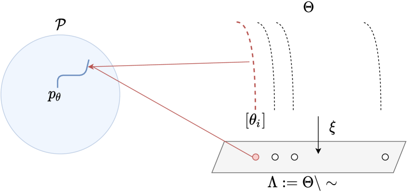
Figure 3: Consider a singular parameter space, $\bm{\Theta}$, where a set of parameters, $[\theta_{i}]$, maps onto the same point on a function $p_{\theta}$ in the probability space ${\mathcal{P}}$. We propose a reparameterization $\xi$ that maps each set of such singular parameters onto a single point in a regular space $\bm{\Lambda}$ that maps onto the same point in the distribution space as the corresponding parameter set in the singular space.

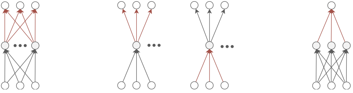
Figure 4: [OP18] (left) we get the overlap singularity directly from equations of the form $g(x|\Theta,\Phi)=\sum_{i}\theta_{i}f(x|\phi_{i})$ which also corresponds to the output of a network layer. (middle) as also described in the introduction we get this from equations of the form $g(x|\theta_{1},\bm{\Phi})=\theta_{1}f(x|\bm{\Phi})$, which we in this case get if the weight matrix becomes zero. (right) for completeness we lastly consider a linear singularity where we show here the setting for $\{\bm{\theta}|\alpha\bm{V}_{1}+\beta\bm{V}_{2}-\bm{V}_{3}=0\}$, where $\alpha,\beta$ are scalars.

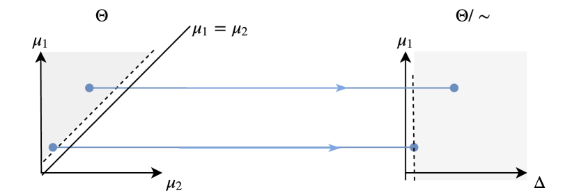
Figure 5: Illustration of the reparameterization of 2-GMM. We see the mapping from the $\{\mu_{1}\neq\mu_{2}\}$ onto $\{\mu_{1},\Delta\}$ and the mapping from $\{\mu_{1}=\mu_{2}+\epsilon\}$ onto $\{\mu_{1},\epsilon\}$. Note that in this description, we exclude mappings from $\mu_{1}=\mu_{2}$ in the figure on the left side, which is equivalent to having a strict $\Delta>0$ on the right-hand side.

Appendix B EM under reparameterization

The following gives the derivation for the $\mu_{1},\Delta$ updates for the M-Step under reparameterization.

Using the reparameterization the 2-GMM can be rewritten as $p(\bm{X}|\eta)=\frac{1}{2}\mathcal{N}\left(\bm{X}|\mu_{1},1\right)+\frac{1}{2}\mathcal{N}\left(\bm{X}|\mu_{1}+\Delta,1\right)$. We want to update $\mu_{1},\Delta$ and therefore consider a constraint optimization under $\Delta>0$. In general terms the setup is as follows: maximize $f(x,y)$ subject to $g(x,y)\leq b$, $b=0$ such that the Lagrangian function [KT51] is $L(x,y,\lambda)=f(x,y)-\lambda[g(x,y)-b]$. If applied to the problem of optimizing the reparameteised mixture we get: $\mathcal{L}(\mu_{1},\Delta,\lambda)=\sum^{N}_{n}z_{n1}(\bm{x}_{n}-\mu_{1})^{2}+z_{n2}(\bm{x}_{n}-(\mu_{1}+\Delta))^{2}-\lambda(-\Delta-0)$ with $f(\mu_{1},\Delta)=\sum^{N}_{n}z_{n1}(\bm{x}_{n}-\mu_{1})^{2}+z_{n2}(\bm{x}_{n}-(\mu_{1}+\Delta))^{2}$ and $g(\mu_{1},\Delta)=-\Delta$ the derivertives $\frac{d}{d\bm{\mu}_{1}}=\sum^{N}_{n}(2\mu_{1}-2\bm{x}_{n})z_{n1}+(2\Delta+2\mu_{1}-2\bm{x}_{n})z_{n2}=0$ and $\frac{d}{d\Delta}=\sum^{N}_{n}(2\Delta+2\mu_{1}-2\bm{x}_{n})z_{n2}+\lambda=0$ and the conditions on the constraints $\lambda(-\Delta-0)=0$, $\lambda\geq 0$ and finally $-\Delta\leq 0$. which gives us the M-Step update:

$$\mu_{1}= \frac{\sum^{N}_{n}z_{n1}\bm{x}_{n}\Delta\sum^{N}_{n}z_{n1}+\sum^{N}_{n}z_{n2}\bm{x}_{n}}{\sum^{N}_{n}z_{n1}+\sum^{N}_{n}z_{n2}}$$

$$\Delta= \frac{\sum^{N}_{n}z_{n2}\bm{x}_{n}-\mu_{1}\sum^{N}_{n}z_{n2}}{\sum^{N}_{n}z_{n2}}$$

Appendix C General ERC under Relative Reparameterization

We can summarize the more general EM algorithm under reparameterization in Algorithm 2.

The E-Step stays the same and in the CM-step in line six, we now consider the update of the reparameterized model.

For this implementation, we consider break criteria in line two of the change in log-likelihood being below a threshold $\varepsilon$. Note that in practice, we only have to define the reparameterization once in the beginning and not go back and forth between the reparameterizations in each iteration. We only include this here to illustrate which parts of the algorithm effectively do not change under the reparameterization.

Algorithm 2 ECM under Relative Reparamterization

Define log likelihood: $\ln\mathcal{L}(\bm{\Theta};\bm{X})$

while $\left\lVert\ln\mathcal{L}(\bm{\Theta}^{(t-1)};\bm{X})-\ln\mathcal{L}(\bm{\Theta}^{(t)};\bm{X})\right\rVert>\varepsilon$ do

     $Q\left(\bm{\theta}|\bm{\theta}^{(t)}\right)=\mathbb{E}_{\mathbf{Z}|\mathbf{X},\bm{\theta}^{(t)}}\left[\ln\mathcal{L}(\bm{\theta};\mathbf{X},\mathbf{Z})\right]$

     $\bm{\theta}^{(t+1)}=\arg\max_{\bm{\theta}}\quad Q\left(\bm{\theta}|\bm{\theta}^{(t)}\right)$

     $\bm{\theta}\stackrel{{\scriptstyle\text{rep.}}}{{\longrightarrow}}\bm{\Lambda}$

     $\bm{\theta}_{1}^{(t+1)}={\arg\max}_{\theta_{1}}\quad Q\left(\bm{\Lambda}|\bm{\Lambda}^{(t)}\right)$

     $\bm{\Delta}^{(t+1)}={\arg\max}_{\bm{\Delta}}\quad Q\left(\bm{\Lambda}|\bm{\Lambda}^{(t)}\right)$

     $\bm{\Lambda}\stackrel{{\scriptstyle\text{rep.}}}{{\longrightarrow}}\bm{\theta}$

end while

Appendix D Derivation of averaged learning dynamcis

In this section we give the full derivation for Section 3.1.

Consider the setting as given in [PO09]. Since the derivation directly follows [PO09] we do not restate the full derivation but only the critical points that change.

Starting from Eq.17, [PO09]

$${\bm{J}} =\begin{bmatrix}1&0&0\\ 0&1&-1\\ u&v&1-v\end{bmatrix}$$

$${\bm{J}}{\bm{J}}^{T} =\begin{bmatrix}1&0&u\\ 0&2&2v-1\\ u&2v-1&2v^{2}-2v+u^{2}+1\end{bmatrix}$$

And under reparametarization we obtain the Jacobian as

$${\bm{J}} =\begin{bmatrix}1&0&0\\ 0&0&1\\ \mu_{1}-\Delta&v+1-\Delta&1-v-\mu_{1}\end{bmatrix}$$

$${\bm{J}}{\bm{J}}^{T} =\begin{bmatrix}1&0&\mu_{1}+\Delta\\ 0&1&1-\Delta-v\\ \mu_{1}+\Delta&v+1-\Delta&3\Delta^{3}+2\mu_{1}\Delta-4\Delta+\mu_{1}^{2}+2v^{2}+2\end{bmatrix}$$

Using a change of variables we can derive the averaged learning equations for the new parameters. This generally corresponds to Eq. 20 - 22 [PO09] but we here compute the exact expressions instead of considering the Taylor approximation. This now gives:

$$\begin{aligned} \mathbb{E}\left[\frac{\mathrm{d}v}{\mathrm{~{}d}t}\right]=&\eta\left(\mathbb{E}\left[\frac{\partial\tilde{l}}{\partial v}\right]+u\mathbb{E}\left[\frac{\partial\tilde{l}}{\partial w}\right]\right)\\ =&-\frac{1}{2}u^{2}(2v-1)\left(w^{2}-2wx+x^{2}-1\right)\\ &-\frac{1}{2}\left(u^{3}\left(6v^{2}-6v+1\right)\left(w^{3}-3w^{2}x+3w\left(x^{2}-1\right)-x\left(x^{2}-3\right)\right)\right)\\ &+u\left(x-w+u^{2}(1-v)v(w-x)-\frac{3}{2}\left(u^{3}v\left(2v^{2}-3v+1\right)\left(w^{2}-2wx+x^{2}-1\right)\right)\right)\\ \mathbb{E}\left[\frac{\mathrm{d}u}{\mathrm{~{}d}t}\right]=&\eta\left(2\mathbb{E}\left[\frac{\partial\tilde{l}}{\partial u}\right]-(1-2v)\mathbb{E}\left[\frac{\partial\tilde{l}}{\partial w}\right]\right)\\ =&2\left(u(1-v)v\left(w^{2}-2wx+x^{2}-1\right)+\frac{3}{2}u^{2}v\left(2v^{2}-3v+1\right)\left((x-w)^{3}+3(w-x)\right)\right)\\ &-(1-2v)\left(-\frac{1}{2}u^{2}(2v-1)\left(w^{2}-2wx+x^{2}-1\right)\right.\\ &-\left.\frac{1}{2}\left(u^{3}\left(6v^{2}-6v+1\right)\left(w^{3}-3w^{2}x+3w\left(x^{2}-1\right)-x\left(x^{2}-3\right)\right)\right)\right)\\ \mathbb{E}\left[\frac{\mathrm{d}w}{\mathrm{~{}d}t}\right]=&\eta\left(u\mathbb{E}\left[\frac{\partial\tilde{l}}{\partial v}\right]-(1-2v)\mathbb{E}\left[\frac{\partial\tilde{l}}{\partial u}\right]+\left(u^{2}+v^{2}+(1-v)^{2}\right)\mathbb{E}\left[\frac{\partial\tilde{l}}{\partial w}\right]\right)\\ =&u\left(-\frac{1}{2}u^{2}(2v-1)\left(w^{2}-2wx+x^{2}-1\right)\right.\\ &\left.-\frac{1}{2}\left(u^{3}\left(6v^{2}-6v+1\right)\left(w^{3}-3w^{2}x+3w\left(x^{2}-1\right)-x\left(x^{2}-3\right)\right)\right)\right)\\ &-(1-2v)\left(-\frac{1}{2}u^{2}(2v-1)\left(w^{2}-2wx+x^{2}-1\right)\right.\\ &-\left.\frac{1}{2}\left(u^{3}\left(6v^{2}-6v+1\right)\left(w^{3}-3w^{2}x+3w\left(x^{2}-1\right)-x\left(x^{2}-3\right)\right)\right)\right)\\ &+\left(u^{2}+v^{2}+(1-v)^{2}\right)\\ &\quad\times\left(x-w+u^{2}(1-v)v(w-x)-\frac{3}{2}\left(u^{3}v\left(2v^{2}-3v+1\right)\left(w^{2}-2wx+x^{2}-1\right)\right)\right)\end{aligned}$$

and similarly under reparameterization (prime notation dropped for readablity).

$$\begin{aligned} \mathbb{E}\left[\frac{\mathrm{d}v}{\mathrm{~{}d}t}\right]&=\eta\left(\mathbb{E}\left[\frac{\partial\tilde{l}}{\partial v}\right]+(\mu_{1}+\Delta)\mathbb{E}\left[\frac{\partial\tilde{l}}{\partial w}\right]\right)\\ =&-\frac{1}{2}u^{2}(2v-1)\left(w^{2}-2wx+x^{2}-1\right)\\ &-\frac{1}{2}\left(u^{3}\left(6v^{2}-6v+1\right)\left(w^{3}-3w^{2}x+3w\left(x^{2}-1\right)-x\left(x^{2}-3\right)\right)\right)\\ &+(\mu_{1}+\Delta)\left(x-w+u^{2}(1-v)v(w-x)-\frac{3}{2}\left(u^{3}v\left(2v^{2}-3v+1\right)\left(w^{2}-2wx+x^{2}-1\right)\right)\right)\\ \mathbb{E}\left[\frac{\mathrm{d}u}{\mathrm{~{}d}t}\right]&=\eta\left(\mathbb{E}\left[\frac{\partial\tilde{l}}{\partial u}\right]-(-v+1-\Delta)\mathbb{E}\left[\frac{\partial\tilde{l}}{\partial w}\right]\right)\\ =&\left(u(1-v)v\left(w^{2}-2wx+x^{2}-1\right)+\frac{3}{2}u^{2}v\left(2v^{2}-3v+1\right)\left((x-w)^{3}+3(w-x)\right)\right)\\ &-(-v+1-\Delta)\left(-\frac{1}{2}u^{2}(2v-1)\left(w^{2}-2wx+x^{2}-1\right)\right.\\ &-\left.\frac{1}{2}\left(u^{3}\left(6v^{2}-6v+1\right)\left(w^{3}-3w^{2}x+3w\left(x^{2}-1\right)-x\left(x^{2}-3\right)\right)\right)\right)\\ \mathbb{E}\left[\frac{\mathrm{d}w}{\mathrm{~{}d}t}\right]&=\eta\left((\mu_{1}+\Delta)\mathbb{E}\left[\frac{\partial\tilde{l}}{\partial v}\right]-(-v+1-\Delta)\mathbb{E}\left[\frac{\partial\tilde{l}}{\partial u}\right]\right.\\ &\ \quad\left.+\left(\mu_{1}^{2}+2\Delta\mu_{1}+3\Delta^{2}+2v^{2}+2-4\Delta\right)\mathbb{E}\left[\frac{\partial\tilde{l}}{\partial w}\right]\right).\\ =&(\mu_{1}+\Delta)\left(-\frac{1}{2}u^{2}(2v-1)\left(w^{2}-2wx+x^{2}-1\right)\right.\\ &\left.-\frac{1}{2}\left(u^{3}\left(6v^{2}-6v+1\right)\left(w^{3}-3w^{2}x+3w\left(x^{2}-1\right)-x\left(x^{2}-3\right)\right)\right)\right)\\ &-(-v+1-\Delta)\left(-\frac{1}{2}u^{2}(2v-1)\left(w^{2}-2wx+x^{2}-1\right)\right.\\ &-\left.\frac{1}{2}\left(u^{3}\left(6v^{2}-6v+1\right)\left(w^{3}-3w^{2}x+3w\left(x^{2}-1\right)-x\left(x^{2}-3\right)\right)\right)\right)\\ &+\left(\mu_{1}^{2}+2\Delta\mu_{1}+3\Delta^{2}+2v^{2}+2-4\Delta\right)\\ &\quad\times\left(x-w+u^{2}(1-v)v(w-x)-\frac{3}{2}\left(u^{3}v\left(2v^{2}-3v+1\right)\left(w^{2}-2wx+x^{2}-1\right)\right)\right)\end{aligned}$$

The above is used to plot Figure LABEL:fig:dynamics_around_0 and Figure LABEL:fig:dynamics_away_from_0.

References

- [AC21] Stéphanie Allassonnière and Juliette Chevallier “A new class of stochastic EM algorithms. Escaping local maxima and handling intractable sampling” In Computational Statistics & Data Analysis, 2021
- [AG16] Anima Anandkumar and Rong Ge “Efficient approaches for escaping higher order saddle points in non-convex optimization” In Journal of Machine Learning Research, 2016
- [Aka74] H. Akaike “A new look at the statistical model identification” In IEEE Transactions on Automatic Control, 1974
- [Ama+18] Shun-ichi Amari, Tomoko Ozeki, Ryo Karakida, Yuki Yoshida and Masato Okada “Dynamics of Learning in Mlp: Natural Gradient and Singularity Revisited” In Neural Computation, 2018
- [Ama98] Shun-Ichi Amari “Natural Gradient Works Efficiently in Learning” In Neural Computation, 1998
- [AMS08] P.-A. Absil, R. Mahony and R. Sepulchre “Optimization Algorithms on Matrix Manifolds” Princeton University Press, 2008
- [APO01] Shun-ichi Amari, Hyeyoung Park and Tomoko Ozeki “Geometrical Singularities in the Neuromanifold of Multilayer Perceptrons” In Proceedings of the 14th International Conference on Neural Information Processing Systems: Natural and Synthetic, 2001
- [APO06] Shun-ichi Amari, Hyeyoung Park and Tomoko Ozeki “Singularities Affect Dynamics of Learning in Neuromanifolds” In Neural Computation, 2006
- [AR85] Murray Aitkin and Donald B. Rubin “Estimation and Hypothesis Testing in Finite Mixture Models” Journal of the Royal Statistical Society, 1985
- [Bon13] Silvere Bonnabel “Stochastic Gradient Descent on Riemannian Manifolds” In IEEE Transactions on Automatic Control, 2013
- [BP66] Leonard E. Baum and Ted Petrie “Statistical Inference for Probabilistic Functions of Finite State Markov Chains” In The Annals of Mathematical Statistics, 1966
- [BV04] Stephen Boyd and Lieven Vandenberghe “Convex Optimization” Cambridge University Press, 2004
- [CH13] Didier Chauveau and David R. Hunter “ECM and MM algorithms for normal mixtures with constrained parameters”, 2013
- [Cho56] Noam Chomsky “Three models for the description of language” In IRE Transactions on Information Theory, 1956
- [CHR00] Gilles Celeux, Merrilee Hurn and Christian P. Robert “Computational and Inferential Difficulties with Mixture Posterior Distributions” In Journal of the American Statistical Association, 2000
- [Cra46] Harald Cramer “Mathematical methods of statistics / by Harald Cramer” Princeton University Press Princeton, 1946
- [DHS11] John Duchi, Elad Hazan and Yoram Singer “Adaptive Subgradient Methods for Online Learning and Stochastic Optimization” In Journal of Machine Learning Research, 2011
- [DLR77] A. P. Dempster, N. M. Laird and D. B. Rubin “Maximum Likelihood from Incomplete Data via the EM Algorithm” In Journal of the Royal Statistical Society. Series B (Methodological), 1977
- [Dwi+18] Raaz Dwivedi, Nhat Ho, Koulik Khamaru, Michael I. Jordan, Martin J. Wainwright and Bin Yu “Singularity, Misspecification, and the Convergence Rate of EM”, 2018
- [ED94] Sean R. Eddy and Richard Durbin “RNA sequence analysis using covariance models” In Nucleic Acids Research, 1994
- [EN21] Pascal Mattia Esser and Frank Nielsen “Towards Modeling and Resolving Singular Parameter Spaces using Stratifolds” In Annual Workshop on Optimization for Machine Learning, 2021
- [FM07] Yu Fujimoto and Noboru Murata “A modified EM algorithm for mixture models based on Bregman divergence” In Annals of the Institute of Statistical Mathematics, 2007
- [GBC16] Ian Goodfellow, Yoshua Bengio and Aaron Courville “Deep Learning” MIT Press, 2016
- [Guo+18] Weili Guo, Yuan Yang, Yingjiang Zhou, Yushun Tan, Haikun Wei, Aiguo Song and Guochen Pang “Influence Area of Overlap Singularity in Multilayer Perceptrons” In IEEE Access, 2018
- [KB14] Diederik Kingma and Jimmy Ba “Adam: A Method for Stochastic Optimization” In International Conference on Learning Representations, 2014
- [KT51] H. W. Kuhn and A. W. Tucker “Nonlinear Programming” In Proceedings of the Second Berkeley Symposium on Mathematical Statistics and Probability Berkeley, Calif.: University of California Press, 1951
- [LC98] Erich L. Lehmann and George Casella “Theory of Point Estimation” Springer-Verlag, 1998
- [Lin+21] Wu Lin, Frank Nielsen, Mohammad Emtiyaz Khan and Mark Schmidt “Tractable structured natural gradient descent using local parameterizations” In International Conference on Machine Learning, 2021
- [Mil85] John Milnor “On the concept of attractor” In Communications in Mathematical Physics, 1985
- [MP00] Geoffrey J. McLachlan and David Peel “Finite mixture models”, 2000
- [MR93] Xiao-Li Meng and Donald B. Rubin “Maximum likelihood estimation via the ECM algorithm: A general framework” In Biometrika, 1993
- [MSMG13] Andrew M. Saxe, James Mcclelland and Surya Ganguli “Exact solutions to the nonlinear dynamics of learning in deep linear neural networks” In International Conference on Learning Representations, 2013
- [MU49] Nicholas Metropolis and S. Ulam “The Monte Carlo Method” In Journal of the American Statistical Association, 1949
- [New86] Simon Newcomb “A Generalized Theory of the Combination of Observations so as to Obtain the Best Result” In American Journal of Mathematics, 1886
- [Nie13] Frank Nielsen “Cramer-Rao Lower Bound and Information Geometry” In Texts and Readings In Mathematics, 2013
- [OP18] Emin Orhan and Xaq Pitkow “Skip Connections Eliminate Singularities” In International Conference on Learning Representations, 2018
- [PO09] Hyeyoung Park and Tomoko Ozeki “Singularity and Slow Convergence of the EM algorithm for Gaussian Mixtures” In Neural Processing Letters, 2009
- [RG02] Sylvia Richardson and P. Green “On Bayesian Analysis of Mixtures With an Unknown Number of Components” In Journal of the Royal Statistical Society: Series B (Statistical Methodology), 2002
- [RHW86] D. E. Rumelhart, G. E. Hinton and R. J. Williams “Parallel Distributed Processing: Explorations in the Microstructure of Cognition, Vol. 1”, 1986
- [Sch78] Gideon Schwarz “Estimating the Dimension of a Model”, 1978
- [SN19] Ke Sun and Frank Nielsen “Lightlike Neuromanifolds, Occam’s Razor and Deep Learning” In CoRR, 2019
- [SS95] David Saad and Sara A. Solla “On-line learning in soft committee machines” In Physical Review E, 1995
- [SSBD14] Shai Shalev-Shwartz and Shai Ben-David “Understanding Machine Learning: From Theory to Algorithms” Cambridge University Press, 2014
- [Ste99] Matthew Stephens “Dealing with Multimodal Posteriors and Non-Identifiability in Mixture Models” In Journal of the Royal Statistical Society, 1999
- [Tak12] Keiji Takai “Constrained EM algorithm with projection method” In Computational Statistics, 2012
- [TH12] T. Tieleman and G. Hinton “Lecture 6.5—RmsProp: Divide the gradient by a running average of its recent magnitude”, COURSERA: Neural Networks for Machine Learning, 2012
- [Tri+18] Nilesh Tripuraneni, Nicolas Flammarion, Francis Bach and Michael I. Jordan “Averaging Stochastic Gradient Descent on Riemannian Manifolds” In Conference On Learning Theory, 2018
- [Vap82] Vladimir Vapnik “Estimation of Dependences Based on Empirical Data” In Springer Series in Statistics, 1982
- [Vap98] V.N. Vapnik “Statistical Learning Theory” In A Wiley-Interscience publication, 1998
- [VDM86] C. Van Der Malsburg “Frank Rosenblatt: Principles of Neurodynamics: Perceptrons and the Theory of Brain Mechanisms” In Brain Theory, 1986
- [VRW86] Raja P. Velu, Gregory C. Reinsel and Dean W. Wichern “Reduced rank models for multiple time series” In Biometrika, 1986
- [Wat09] Sumio Watanabe “Algebraic Geometry and Statistical Learning Theory” Cambridge University Press, 2009
- [Wat10] Sumio Watanabe “Asymptotic Equivalence of Bayes Cross Validation and Widely Applicable Information Criterion in Singular Learning Theory” In Journal of Machine Learning Research, 2010
- [Wat13] Sumio Watanabe “A Widely Applicable Bayesian Information Criterion” In Journal of Machine Learning Research, 2013
- [Wei+08] Haikun Wei, Jun Zhang, Florent Cousseau, Tomoko Ozeki and Shun Amari “Dynamics of Learning Near Singularities in Layered Networks” In Neural Computation, 2008
- [Wes97] Mike West “Hierarchical Mixture Models in Neurological Transmission Analysis” In Journal of the American Statistical Association, 1997
- [Wil70] Stephen Willard “General topology” Reading, Mass. : Addison-Wesley Pub. Co., 1970
- [Wu83] C. F. Jeff Wu “On the Convergence Properties of the EM Algorithm” In The Annals of Statistics, 1983
- [XJ96] Lei Xu and Michael I. Jordan “On Convergence Properties of the Em Algorithm for Gaussian Mixtures” In Neural Computation, 1996