Inelastic nuclear scattering from neutrinos and dark matter

Abstract

Neutrinos with energy of order 10 MeV, such as from pion decay-at-rest sources, are an invaluable tool for studying low-energy neutrino interactions with nuclei – previously enabling the first measurement of coherent elastic neutrino-nucleus scattering. Beyond elastic scattering, neutrinos and dark matter in this energy range also excite nuclei to its low-lying nuclear states, providing an additional physics channel. Here, we consider neutral-current inelastic neutrino-nucleus and dark matter(DM)-nucleus scattering off ⁴⁰Ar, ¹³³Cs, and ¹²⁷I nuclei that are relevant to a number of low-threshold neutrino experiments at pion decay-at-rest facilities. We carry out large scale nuclear shell model calculations of the inelastic cross sections considering the full set of electroweak multipole operators. Our results demonstrate that Gamow-Teller transitions provide the dominant contribution to the cross section and that the long-wavelength limit provides a reasonable approximation to the total cross section for neutrino sources. We show that future experiments will be sensitive to this channel and thus these results provide additional neutrino and DM scattering channels to explore at pion decay-at-rest facilities.

I Introduction

The large flux of neutrinos produced as a by-product at spallation neutron sources has enabled new tests of the Standard Model of particle physics. Most notably, the first measurement of coherent elastic neutrino nucleus scattering (CE$\nu$NS) by the COHERENT collaboration at the Spallation Neutron Source (SNS) in 2017 [1]. Several other CE$\nu$NS experiments have been completed or are in operation, such as Coherent CAPTAIN-Mills (CCM) at Los Alamos National Laboratory (LANL) [2]. Additional measurements have improved in precision and thus far they are in agreement with the Standard Model (SM) predictions [3]. Further improvements in precision will allow these experiments to probe physics beyond the SM, e.g. non-standard neutrino interactions [4, 5, 6, 7, 8, 9, 10, 11, 12, 13, 14, 15, 16] and dark matter [17, 18, 19, 20, 21, 22, 23, 24].

Other SM signals that could be observable at these experiments include inelastic neutrino-nucleus scattering, where the nucleus is left in an excited state. Neutrinos with energies of tens of MeV can excite many states in the various target nuclei used for these experiments. While the cross section for inelastic scattering is much smaller than the coherently enhanced elastic scattering, these processes could provide unique tests of new physics and/or important backgrounds to new physics searches. Additionally, understanding inelastic neutrino-nucleus scattering is also vital for the detection of core-collapse supernova signals by the next generation neutrino experiments, such as DUNE [25] and Hyper-K [26]. At present there are very few existing measurements of inelastic neutrino-nucleus cross sections in this energy regime, leaving them poorly understood. The measurements that exist are primarily for carbon and iron targets performed by the KARMEN [27] and LSND [28] collaborations, none at better than the 10% uncertainty level. Presently no measurement has been made for scattering on the argon nucleus. Theoretical understanding of these processes is also relatively poor, due to strong dependence of the interaction rates on the specific initial- and final-state nuclear wavefunctions and require cumbersome computation to account for underlying complex nuclear structure. It is therefore important to have good theoretical estimates of their rates employing fast and efficient computational methods.

A number of theoretical approaches have been used in the past to calculate inelastic neutrino-nucleus scattering [29, 30, 31, 32, 33, 34, 35, 36, 37, 38, 39] although with more attention paid to the charged current processes. Additionally, not much attention has been paid to nuclei that are relevant to the current low-energy neutrino experiments, e.g., argon and cesium. More recent studies of neutral current inelastic processes have been presented, e.g., within the continuum Random Phase Approximation (CRPA) method [40, 41], the deformed shell model mixed with the free nucleon approximation [42], and merely free nucleon approximation [43]. The CRPA model employs long-range correlations among nucleons on top of a Hartree-Fock picture of the nucleus and predicts cross sections above the nucleon emission threshold utilizing a multipole expansion [44, 45]. This method to date provides predictions of inclusive cross sections, not cross sections for specific final states which are required for predicting detailed experimental signatures. The free nucleon approximation is particularly inaccurate in the calculation of inelastic scattering in this energy range since it ignores nuclear structure. While Ref. [42] does employ the deformed shell model to include nuclear structure effects, their results only consider the first excited state. In this work we provide the first comprehensive calculation of neutral current (NC) inelastic neutrino-nucleus scattering using electroweak theory and the nuclear shell model, and extend it to describe inelastic DM-nucleus scattering in a consistent manner.

Low-energy beam based neutrino experiments (CCM, COHERENT, etc.) provide a great opportunity to probe well-motivated light dark matter via light mediators, where the timing information is utilized to control the SM neutrino background. The high-intensity proton beam impacts a target producing a high-intensity flux of photons from cascades, meson decays and pion absorption [46]. These photons can then produce light vector mediators via kinetic mixing, while scalar mediators can be produced from three-body decays of charged pions [47]. The light mediators decay promptly into a pair of DM particles which can then produce signals via nuclear recoils in the detector. For proton beams with $E_{p}\sim 1$ GeV the resulting energy of light DM particles is $\sim$ $\mathrm{O}$(50-100) MeV. Like the neutrinos, the DM particles will also initiate inelastic DM-nucleus scattering. Here, the inelastic scatters involve relativistic DM unlike the non-relativistic DM-nucleus scattering in direct detection experiments, previously explored in [48, 49]. In this paper we evaluate these cross sections fully relativistically using electroweak multipole operators, with special attention to the long-wavelength limit Gamow Teller operator.

The DM-nucleus inelastic scattering process is mediated by a neutral dark photon only and thus the NC neutrino-nucleus scattering process will be an important and irreducible background for any accelerator based DM searches using this channel.

The paper is organized as follows, in section II we describe neutrino-nucleus scattering within the electroweak multipole framework, in section III we extend this to the case of DM-nucleus scattering, in section IV we present the shell-model calculation results for the cross sections, in section V, we discuss scattering rates and experimental signatures and lastly, in section VI we conclude.

II Neutrino-nucleus scattering

II.1 Electroweak multipole operators

At sufficiently small momentum transfer (where $q<100$ MeV), neutrinos coherently scatter from nuclei which, in the case of elastic scattering, greatly enhances the cross section. As shown in Fig. 1, the scattering process involves the exchange of a $Z$ boson, where the outgoing nucleus $N^{*}$ could be in the ground state (for elastic scattering) or an excited state (for inelastic scattering). Inelastic scattering can also proceed via a charged current interaction, in which case the outgoing nucleus will have a different atomic number. In this work we will only consider neutral current scattering.

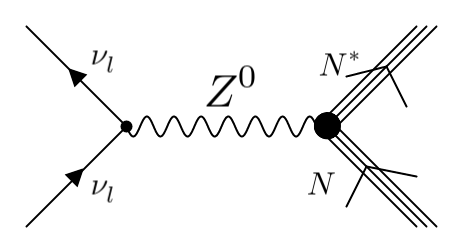
Figure 1: The inelastic neutral current neutrino-nucleus scattering process where a $Z^{0}$ boson is exchanged between neutrino ($\nu_{l}$) and the target nucleus ($N$).

The differential cross section for the CE$\nu$NS process is conventionally calculated assuming that the protons and neutrons are distributed equally within the nucleus, it then takes the form:

$$\frac{d\sigma^{\nu}_{\rm el}}{dE_{r}} = \frac{G_{F}^{2}}{4\pi}m_{N}\left(1-\frac{E_{r}}{E_{\nu}}-\frac{m_{N}E_{r}}{2E_{\nu}^{2}}\right)$$ (1)

$$\times\left[(1-4\sin^{2}\theta_{W})Z-N\right]^{2}F_{W}^{2}(q^{2})$$

where $m_{N}$ is the target nucleus mass, $E_{\nu}$ is the incoming neutrino energy, $E_{r}$ is the nuclear recoil energy, $Z$ ($N$) is the target’s atomic (neutron) number, $F_{W}(q^{2})$ is the weak form factor of the nucleus, and $\theta_{W}$ is the Weinberg angle. A common parameterization for the form factor is the Helm form [50]. Given the value of $\sin^{2}\theta_{W}\approx 0.23$, the CE$\nu$NS cross section scales approximately as the number of neutrons squared in the target nucleus, and (not including small radiative corrections) is independent of the neutrino flavor. Efforts to improve the CE$\nu$NS cross section calculation through a more detailed treatment of the hadronic current which allows for sub-leading nuclear structure effects was included in Ref. [51] while radiative corrections were added in Ref. [52].

In the context of low-energy CE$\nu$NS experiments, the inelastic scattering of neutrinos has not received much attention - potentially owing to its smaller cross section which is not coherently enhanced. Previous attempts to estimate the inelastic neutrino-nucleus scattering rates have not used detailed nuclear calculations [43] or only explored the lowest lying states [42]. In this work we apply the formalism of semi-leptonic electroweak theory as developed in [53, 54, 55] to the calculation of inelastic neutrino-nucleus scattering. In this formalism the relevant hadronic current is spherically decomposed and expanded in multipoles to obtain irreducible tensor operators which act on single particle states, which can generically be expressed as an expansion of harmonic oscillator states [55]. This is a convenient basis to work in, since it results in single-particle matrix elements that are polynomials of the momentum transfer. Following [56], in the extreme relativistic limit the total cross section can be written as:

$$\left(d\sigma\over d\Omega\right)_{\nu,\bar{\nu}} =\frac{2G_{F}^{2}}{\pi(2J_{i}+1)}E_{f}^{2}\,\cos^{2}{{\theta\over 2}}\Bigg{\{}\sum_{J=0}^{\infty}|\langle J_{f}||\hat{\mathcal{M}}_{J}+\frac{q_{0}}{q}\hat{\mathcal{L}}_{J}||J_{i}\rangle|^{2}$$

$$+\left[-{q_{\mu}^{2}\over 2q^{2}}+\tan^{2}{{\theta\over 2}}\right]\sum_{J=1}^{\infty}\left[|\langle J_{f}||\hat{\mathcal{T}}_{J}^{el}||J_{i}\rangle|^{2}+|\langle J_{f}||\hat{\mathcal{T}}_{J}^{mag}||J_{i}\rangle|^{2}\right]$$

$$\mp 2\tan{{\theta\over 2}}\left[-{q_{\mu}^{2}\over q^{2}}+\tan^{2}{{\theta\over 2}}\right]^{1/2}\sum_{J=1}^{\infty}{\rm Re}\left(\langle J_{f}||\hat{\mathcal{T}}_{J}^{mag}||J_{i}\rangle\langle J_{f}||\hat{\mathcal{T}}_{J}^{el}||J_{i}\rangle^{*}\right)\Biggr{\}}$$ (2)

where $J_{i/f}$ is the initial/final nuclear spin, $E_{f}=E_{\nu}-\omega$ is the outgoing neutrino energy, $\theta$ is the scattering angle, $\omega=\Delta E+E_{r}\approx\Delta E$(excitation energy), $q^{\mu}=(q_{0},\textbf{q})$ is the 4-momentum transfer with $q_{0}=E_{\nu}-E_{f}$ and $q=|\textbf{q}|=\sqrt{2m_{N}E_{r}}$ (for a nuclear recoil energy of $E_{r}$). The electroweak multipole operators are projections of the weak hadronic current, $\hat{\mathcal{J}}$, such that they can act on nuclear states with good angular momentum and parity, they are defined by

$$\hat{\mathcal{M}}_{JM} = \hat{M}_{JM}+\hat{M}^{5}_{JM}$$

$$= \int d^{3}x[j_{J}(qx)Y_{JM}(\Omega_{x})]\hat{\mathcal{J}}_{0}(x)$$

$$\hat{\mathcal{L}}_{JM} = \hat{L}_{JM}+\hat{L}_{JM}^{5}$$

$$= \frac{i}{q}\int d^{3}x\left[\nabla[j_{J}(qx)Y_{JM}(\Omega_{x})]\right]\cdot\hat{\mathcal{J}}(x)$$

$$\hat{\mathcal{T}}_{JM}^{\rm el} = \hat{T}^{\rm el}_{JM}+\hat{T}_{JM}^{\rm el5}$$

$$= \frac{1}{q}\int d^{3}x[\nabla\times j_{J}(qx)\textbf{Y}^{M}_{JJ1}(\Omega_{x})]\cdot\hat{\mathcal{J}}(x)$$

$$\hat{\mathcal{T}}_{JM}^{\rm mag} = \hat{T}_{JM}^{\rm mag}+\hat{T}_{JM}^{\rm mag5}$$ (3)

$$= \int d^{3}x[j_{J}(qx)\textbf{Y}^{M}_{JJ1}(\Omega_{x})]\cdot\hat{\mathcal{J}}(x)$$

where $j_{J}(qx)$ are Bessel functions, $Y_{JM}(\Omega_{x})$ are spherical harmonics and $\textbf{Y}^{M}_{JJ1}(\Omega_{x})$ are vector spherical harmonics. The weak hadronic current has V-A structure $\hat{\mathcal{J}}_{\mu}=\hat{J}_{\mu}+\hat{J}_{\mu}^{5}$, allowing the operators to be split into components of normal and abnormal parity. The normal parity operators: $M_{JM},L_{JM},T^{el}_{JM},$ and $T_{JM}^{mag5}$ can only contribute to transitions with $\Delta\pi=(-1)^{J}$. Similarly only $M^{5}_{JM},L^{5}_{JM},T^{el5}_{JM},$ and $T_{JM}^{mag}$ can contribute to abnormal parity transitions $\Delta\pi=(-1)^{J+1}$. At the one-body level, the vector and axial multipole operators can be expressed in terms of the 7 single-particle operators and nucleon form factors (see [57] for further details):

$$M_{JM} = F_{1}^{N}(q_{\mu}^{2})M_{J}^{M}$$

$$L_{JM} = \frac{q_{0}}{q}M_{JM}$$

$$T^{\rm el}_{JM} = {q\over m_{n}}(F_{1}^{N}(q_{\mu}^{2})\Delta^{{}^{\prime}M}_{J}+{\textstyle{1\over 2}}\mu^{N}(q_{\mu}^{2})\Sigma^{M}_{J})$$

$$T^{\rm mag}_{JM} = -{iq\over m_{n}}(F_{1}^{N}(q_{\mu}^{2})\Delta_{J}^{M}-{\textstyle{1\over 2}}\mu^{N}(q_{\mu}^{2})\Sigma_{J}^{{}^{\prime}M})$$

$$M^{5}_{JM} = {iq\over m_{n}}(G_{A}^{N}(q_{\mu}^{2})\Omega_{J}^{{}^{\prime}M}+{\textstyle{1\over 2}}q_{0}G_{P}^{N}(q_{\mu}^{2})\Sigma^{{}^{\prime\prime}M}_{J})$$

$$L_{JM}^{5} = i\left(G_{A}^{N}(q_{\mu}^{2})-{q^{2}\over 2m_{n}}G_{P}^{N}(q_{\mu}^{2})\right)\Sigma^{{}^{\prime\prime}M}_{J}$$

$$T_{JM}^{\rm el5} = iG_{A}^{N}(q_{\mu}^{2})\Sigma^{{}^{\prime}M}_{J}$$

$$T_{JM}^{\rm mag5} = G_{A}^{N}(q_{\mu}^{2})\Sigma^{M}_{J}$$ (4)

where $m_{n}$ is the nucleon mass, $\mu^{N}(q_{\mu}^{2})=F_{1}^{N}(q_{\mu}^{2})+2m_{n}F_{2}^{N}(q_{\mu}^{2})$ is the magnetic moment, and $F_{1}(q_{\mu}^{2})$, $F_{2}(q_{\mu}^{2})$, $G_{A}(q_{\mu}^{2})$ and $G_{P}(q_{\mu}^{2})$ are the Dirac, Pauli, axial and pseudoscalar neutral current nucleon form factors. In the low recoil-energy limit, these become [51]:

$$F_{1}^{n}(0)= 0\;\;\;\; F_{1}^{p}(0)=1$$

$$F_{2}^{n}(0)= -1.91\;\;\;\; F_{2}^{p}(0)=1.79$$

$$G_{A}^{n}(0)= -g_{A}/2\;\;\;\; G_{A}^{p}(0)=g_{A}/2$$

$$G_{P}^{n}(0)= {2m_{n}G_{A}^{n}(0)\over m_{\pi}^{2}}\;\;\;\; G_{P}^{p}(0)={2m_{n}G_{A}^{p}(0)\over m_{\pi}^{2}}$$

The energy dependence of the axial form factor $G_{A}$ is conventionally taken to have a dipole form [58],

$$G_{A}(q^{2})=\frac{g_{A}}{(1+\,q^{2}/\Lambda_{A}^{2})^{2}}$$ (5)

where $g_{A}=1.27$ and the axial mass is $\Lambda_{A}\approx 1040$ MeV. In this work the scattering processes we consider have low momentum transfer, $q^{2}\ll\Lambda_{A}^{2}$, and thus the $q^{2}$ dependence of $F_{A}$ can be neglected.

The results of the the single particle operators acting on harmonic oscillator basis states have been tabulated in [59]. In this work we use the SevenOperators code to evaluate and simplify the relevant matrix elements [57]. Sometimes it is desirable to have the differential cross section in Eq. (2) written in terms of recoil energy, i.e. $\frac{d\sigma}{dE_{r}}=\frac{d\sigma}{d\Omega}\frac{d\Omega}{dE_{r}}=2\pi\frac{d\sigma}{d\Omega}\frac{m_{N}}{E_{i}E_{f}}$.

In this analysis we consider only one-body currents, however, there are likely significant contributions from two-body currents [51].

II.2 Gamow–Teller transitions

For small momentum transfers, when a Gamow-Teller (GT) transition is kinematically accessible, the inelastic cross section will be dominated by such allowed GT transitions. We can see this by looking at Eq. (3) in the long-wavelength limit. The only surviving multipoles are $\hat{\mathcal{M}}_{00}$, $\hat{\mathcal{T}}^{el}_{1M}$ and $\hat{\mathcal{L}}_{1M}$. With $\hat{\mathcal{L}}$ further suppressed by $q$ in the cross section (see Eq. (2)), we need only consider the first two operators. The $\hat{\mathcal{M}}_{00}$ and $\hat{\mathcal{T}}^{el}_{1M}$ operators are associated with Fermi operator, $\hat{\tau_{0}}$, and GT operator, $\frac{1}{2}\hat{\sigma_{i}}\hat{\tau_{0}}$, respectively:

$$\hat{\mathcal{M}}_{00} = \frac{1}{\sqrt{4\pi}}F_{1}\,\,\sum_{i=1}^{A}\hat{FT}$$ (6)

$$\hat{\mathcal{T}}^{el}_{1M} = \sqrt{2}\hat{\mathcal{L}}_{1M}=\frac{i}{\sqrt{6\pi}}G_{A}\,\,\sum_{i=1}^{A}\hat{GT}.$$ (7)

In the long-wavelength limit the GT operator allows transitions with $|\Delta J|=1$, while the Fermi operator allows $\Delta J=0$ transitions. For inelastic scattering, $\Delta J=0$ transitions are possible only if a nucleon can be excited to a state of the same $l$ but higher $n$ (since conserving $J$ but changing $l$ by 1 is disallowed by parity conservation). For the model spaces we consider such a transition does not exist. So while such a possibility is allowed by our multipole calculation, it does not contribute here.

Therefore, considering the GT operator alone in the long wavelength limit can provide an efficient way to approximate the scattering cross section. In the multipole operator analysis the GT operator is contained within $\hat{T}_{J}^{el5}$. The relevant part of the cross section in Eq. (2) is:

$${{d\sigma^{\rm GT}\over d\Omega}} =\frac{2G_{F}^{2}}{\pi(2J+1)}E_{f}^{2}\,\cos^{2}{{\theta\over 2}}$$

$$\times\left(-{q_{\mu}^{2}\over 2q^{2}}+\tan^{2}{{\theta\over 2}}\right)\sum_{J=1}^{\infty}|\langle J_{f}||\hat{T}_{J}^{el5}||J_{i}\rangle|^{2}.$$ (8)

Taking the long–wavelength limit ($q\rightarrow 0$, or equivalently $E_{r}\rightarrow 0$) gives $G_{A}\approx g_{A}$ and ignores the momentum dependence of the nuclear form factor, the amplitude can then be simplified to:

$$\bigl{|}\langle J_{f}||\sum_{J=1}^{\infty}\hat{T}_{J}^{el5}||J_{i}\rangle\bigr{|}^{2}\approx\frac{g_{A}^{2}}{6\pi}\bigl{|}\langle J_{f}||\sum_{i=1}^{A}\frac{1}{2}\hat{\sigma_{i}}\hat{\tau_{0}}||J_{i}\rangle\bigr{|}^{2}.$$ (9)

Substituting this into Eq. (II.2) allows us to write the cross section as

$${d\sigma^{\rm GT}\over\ d\cos\theta} \approx\frac{G_{F}^{2}g_{A}^{2}}{2\pi(2J+1)}(E_{\nu}-\Delta E)^{2}\left(1-\frac{1}{3}\,\cos\theta\right)$$ (10)

$$\times|\langle J_{f}||\sum_{i=1}^{A}\frac{1}{2}\hat{\sigma_{i}}\hat{\tau_{0}}||J_{i}\rangle|^{2}$$

where we have written the final neutrino energy in terms of the incoming neutrino energy, $E_{\nu}$, and the final state excitation energy, $\Delta E$, which is assumed to be small in this approximation. We can then make connection with the common form of the cross section for neutral current GT transitions by integrating Eq. (10) to find the total cross section:

$$\sigma^{GT}_{\nu}\approx\frac{G_{f}^{2}g_{A}^{2}}{\pi(2J+1)}(E_{\nu}-\Delta E)^{2}|\langle J_{f}||\sum_{i=1}^{A}\frac{1}{2}\hat{\sigma_{i}}\hat{\tau_{0}}||J_{i}\rangle|^{2}.$$ (11)

This form of the cross section is in agreement with others found in the literature [60, 61]. We will see in a later section that using Eq. (11) to calculate the cross section will allow for an important simplification of the numerical many-body problem while providing an adequate estimation of the transition matrix elements in the long wavelength limit.

III Dark matter-nucleus scattering

In this section we apply the formalism discussed in the preceding section to the inelastic scattering of dark matter (DM) on nuclei. Previous analyses considered the scattering of nonrelativistic dark matter [42, 62, 63], which greatly restricts the excited states that are accessible. Astrophysically, dark matter can be boosted via several mechanisms, however the flux will be subdominant compared to the non-relativistic component. Larger fluxes of boosted dark matter could be produced in the decay of particles produced in collider experiments such as [1, 2].

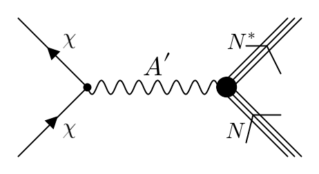
Figure 2: Scattering of a DM particle, $\chi$, from a nucleus, $N$, mediated via a dark photon, $A^{\prime}$.

Low-energy beam dump experiments can investigate light dark matter where the light dark matter interacts with the SM particle via light mediators. In these experiments neutrinos are produced as a product of stopped-pion decay, but they are also high-intensity sources of photons emerging from meson decays and cascades which could produce exotic light vector mediators via kinetic mixing. The light vector mediators can then promptly decay into a pair of dark matter particles ($\chi,\bar{\chi}$) which are semirelativistic. There exist many well motivated models where this scenario is possible [64, 65, 66, 67, 18, 68, 69, 70, 71, 72]. As a benchmark example we will consider a dark photon A-prime ($A^{\prime}$) model where the $A^{\prime}$ undergoes kinetic mixing with the SM photon. The model is described by the Lagrangian:

$$\mathcal{L}\supset g_{D}A^{\prime}_{\mu}\bar{\chi}\gamma^{\mu}\chi+e\epsilon Q_{q}A^{\prime}_{\mu}\bar{q}\gamma^{\mu}q$$ (12)

where $g_{D}$ is the dark coupling constant, $\epsilon$ is the mixing parameter, $Q_{q}$ is quark’s electric charge. The dark photon will be produced in the processes of pion capture, pion decay and the photons emerging from the cascades:

$$\pi^{-}+p \rightarrow n+A^{\prime}$$ (13)

$$\pi^{+}+n \rightarrow p+A^{\prime}$$ (14)

$$\pi^{0} \rightarrow \gamma+A^{\prime}$$ (15)

Via these processes the SNS, for example, produces dark photons at a rate of $\epsilon^{2}\times 0.23\times 10^{20}$ per day, mostly from $\pi^{0}$ decay. The dark photons then decay to DM: $A^{\prime}\rightarrow\chi\bar{\chi}$. Previous analyses looked at the elastic scattering of such DM from nuclei in the COHERENT detectors [46], here we extend upon this to include inelastic scattering.

The scattering of DM from nuclei proceeds via the exchange of a dark photon, as depicted in Fig. 2. The cross section of elastic DM-nucleus scattering is given by [73]:

$$\frac{d\sigma^{DM}_{\rm el}}{dE_{r}} =\frac{e^{2}\epsilon^{2}g_{D}^{2}Z^{2}}{4\pi(E_{\chi}^{2}-m_{\chi}^{2})(2m_{N}E_{r}+m_{A^{\prime}}^{2})^{2}}F^{2}(q^{2})$$

$$\times \left[2E_{\chi}^{2}m_{N}\left(1-\frac{E_{r}}{E_{\chi}}-\frac{m_{N}E_{r}}{2E_{\chi}^{2}}\right)+E_{r}^{2}m_{N}\right]$$ (16)

where $E_{\chi}/p_{\chi}$ is the energy/momentum of the incoming DM, and $F(q^{2})$ denotes the nuclear form factor. We assume the $A^{\prime}$ decays promptly into a pair of DM particles in this work.

Following the multipole formalism discussed in the previous section, the inelastic cross section is found to be

$$\begin{split}\frac{d\sigma^{DM}_{\rm inel}}{dE_{r}}&=\frac{2e^{2}\epsilon^{2}g_{D}^{2}{E^{\prime}}_{\chi}^{2}}{p_{\chi}{p^{\prime}}_{\chi}(2m_{N}E_{r}+m_{A^{\prime}}^{2})^{2}}\frac{m_{N}}{2\pi}\frac{4\pi}{2J+1}\Bigg{\{}\sum_{J\geqslant 1,spin}\left[\frac{1}{2}(\vec{l}\cdot\vec{l}^{*}-l_{3}l_{3}^{*})\left(\bigl{|}\langle J_{f}||\hat{\mathcal{T}}_{J}^{mag}||J_{i}\rangle\bigr{|}^{2}+\bigl{|}\langle J_{f}||\hat{\mathcal{T}}_{J}^{el}||J_{i}\rangle\bigr{|}^{2}\right)\right]\\ &+\sum_{J\geqslant 0,spin}\left[l_{0}l_{0}^{*}\,\bigl{|}\langle J_{f}||\hat{\mathcal{M}}_{J}||J_{i}\rangle\bigr{|}^{2}+l_{3}l_{3}^{*}\,\bigl{|}\langle J_{f}||\hat{\mathcal{L}}_{J}||J_{i}\rangle\bigr{|}^{2}-2\,l_{3}l_{0}^{*}Re\left(\,\langle J_{f}||\hat{\mathcal{L}}_{J}||J_{i}\rangle\langle J_{f}||\hat{\mathcal{M}}_{J}||J_{i}\rangle^{*}\right)\right]\Bigg{\}}\end{split}$$ (17)

where $E_{\chi}^{\prime}$ and $p_{\chi}^{\prime}$ are the outgoing DM energy and momentum. While the neutrino current contained an axial component, the DM current is purely vector: $l_{\mu}=\bar{\chi}\gamma^{\mu}\chi$. The dark matter current terms $\sum\limits_{s_{i},s_{f}}l_{\mu}l_{\nu}^{*}$ of Eq. (17) evaluate to:

$$\sum\limits_{s_{i},s_{f}}l_{0}l_{0}^{*}=1+\frac{1}{4E_{\chi}{E^{\prime}}_{\chi}}\left(2p_{\chi}^{2}+2{p^{\prime}}_{\chi}^{2}-4m_{N}E_{r}+m_{\chi}^{2}\right)$$

$$\sum\limits_{s_{i},s_{f}}l_{3}l_{3}^{*}=1+\frac{1}{E_{\chi}{E^{\prime}}_{\chi}}\left[-{3\over 2}\left(p_{\chi}^{2}+{p^{\prime}}_{\chi}^{2}\right)+3m_{N}E_{r}-{m_{\chi}^{2}\over 4}\right]$$

$$\sum\limits_{s_{i},s_{f}}l_{3}l_{0}^{*}=-\left({p_{\chi}^{2}+{p^{\prime}}_{\chi}^{2}-2m_{N}E_{r}\over 2p_{\chi}E_{\chi}}+{p_{\chi}\over E_{\chi}}\right)$$

$$\sum\limits_{s_{i},s_{f}}\vec{l}\cdot\vec{l}^{*}=3-{1\over E_{\chi}{E^{\prime}}_{\chi}}\left[{1\over 2}\left(p_{\chi}^{2}+{p^{\prime}}_{\chi}^{2}-2m_{N}E_{r}\right)+{3m_{\chi}^{2}\over 4}\right]$$

$$\sum\limits_{s_{i},s_{f}}(\vec{l}\times\vec{l}^{*})_{3}=0$$ (18)

Further details of the current calculation is given in appendix A.

As in the case of neutrino-nucleus scattering, the elastic cross section receives a coherent enhancement, in this case by a factor of $Z^{2}$ because the dark photon couples to the electromagnetic current. Therefore, the ratio of elastic to inelastic events will be larger in light nuclei (e.g. Ar) and smaller in heavy nuclei (e.g. Cs and I). This is the reverse of the neutrino case (which dominantly couple to neutrons); a feature that could aid in differentiating a dark matter signal from the neutrino background.

Similar to neutrino scattering, we can write down the differential cross section for inelastic DM scattering via the GT operator:

$$\frac{d\sigma^{GT}_{DM}}{dE_{r}} =\frac{2e^{2}\epsilon^{2}g_{D}^{2}{E^{\prime}}_{\chi}^{2}}{p_{\chi}p_{\chi}^{\prime}(2m_{N}E_{r}+m_{A^{\prime}}^{2})^{2}}\frac{m_{N}}{2\pi}\frac{4\pi}{2J+1}$$ (19)

$$\times\biggl{[}\frac{(\vec{l}\cdot\vec{l}^{*}-l_{3}l_{3}^{*})}{2}|\langle J_{f}||\hat{\mathcal{T}}_{J}^{el5}||J_{i}\rangle|^{2}$$

$$+l_{3}l_{3}^{*}\,\bigl{|}\langle J_{f}||\hat{\mathcal{L}}_{J}||J_{i}\rangle\bigr{|}^{2}\biggr{]}.$$

Combining Eq. (7) and Eq. (19) then gives:

$$\frac{d\sigma^{GT}_{DM}}{dE_{r}} =\frac{2e^{2}\epsilon^{2}g_{D}^{2}{E^{\prime}}_{\chi}^{2}}{p_{\chi}p_{\chi}^{\prime}(2m_{N}E_{r}+m_{A^{\prime}}^{2})^{2}}\frac{m_{N}}{2\pi}\frac{4\pi}{2J+1}$$ (20)

$$\times\frac{\vec{l}\cdot\vec{l}^{*}}{2}\frac{g_{A}^{2}}{6\pi}|\langle J_{f}||\sum_{i=1}^{A}\frac{1}{2}\hat{\sigma_{i}}\hat{\tau_{0}}||J_{i}\rangle|^{2}.$$

In principle one can integrate the differential cross section over $E_{r}$ to get the total cross section, however, in this case a closed form expression of Eq. (17) could not be obtained.

IV Shell model calculations

IV.1 Computational details

We compute the cross sections of inelastic neutrino/DM-nucleus scattering for ⁴⁰Ar, ¹³³Cs, and ¹²⁷I nuclei since these nuclear targets are utilized at the ongoing COHERENT and CCM experiments. Two approaches to the calculation are taken: the full multipole operator analysis and the GT transition in the long wavelength limit. For both approaches we use the nuclear shell model code BIGSTICK [74, 75] to solve the many-body problem. In general BIGSTICK supports computing not only low-lying states and their density matrices, but also the strength of arbitrary operators with a well-defined basis, e.g. the GT operator. To evaluate the cross sections using the multipole analysis the full nuclear one-body density matrix is required, which BIGSTICK can generate for converged eigenstates. We use one-body density matrices as defined in BIGSTICK:

$$\rho^{fi}_{K}(a^{\dagger}b)={1\over 2K+1}\langle J_{f}||(a^{\dagger}b)_{K}||J_{i}\rangle$$ (21)

where, following Edmonds and Sakurai, the reduced matrix elements are defined as:

$$\langle J_{f}||O_{K}||J_{i}\rangle={\langle J_{f}M_{f},KM|J_{i}M_{i}\rangle^{-1}\over 2J_{f}+1}\langle J_{f}M_{f}|O_{K}M|J_{i}M_{i}\rangle.$$ (22)

The multipole operator matrix elements can then be computed with the aid of the Mathematica package SevenOperators [57]. Because this approach requires converged eigenstates, it is time and memory consuming if one is interested in many final states. For the restricted case of the GT transition one can use the simpler and more efficient Lanczos strength function [76, 77, 78], which is directly incorporated into BIGSTICK. After $n$ iterations this method can accurately estimate the $n^{th}$ moment of the distribution. Since we do not require the full convergence of the Lanczos algorithm, only convergence of the integrals over the strengths (i.e. $\int S(E)dE=\sum_{J_{f}}|\langle J_{f}||\hat{O}||J_{i}\rangle|^{2}$) this method is highly efficient.

While computing the full density matrix will give more accurate results (including contributions for all operators), we find that the GT strength is sufficiently precise for our purposes. Importantly, when dealing with a large number of final states, it makes the calculation a tractable computational task. While one can perform the strength function calculation for any well-defined operator, we limit ourselves to considering the GT operator which is dominant in the long-wavelength limit. Moreover, it is challenging to explicitly find the basis $\langle a|\hat{O}|b\rangle$ for the other multipole operators.

When computing density matrices we are able to calculate the transition from the ground state to the, for example, $N=2{\,\text{-}\,}16$ excited states of ⁴⁰Ar, which should align well with the lowest lying experimental nuclear energy levels. In comparison, when computing the GT transition with the strength function method, we are able to calculate the strengths of up to $N=500$ states (including states with zero strength). However, since this method doesn’t have fully converged states, these states are drawn from a wider range of energies.

For ¹³³Cs and ¹²⁷I, the nucleons are in the orbits $0g_{7/2}$, $1d_{5/2}$, $0h_{11/2}$, $1d_{3/2}$, $2s_{1/2}$ and we use jj55pna interaction [79]. ⁴⁰Ar has a more challenging nucleon configuration; the protons (10) are in $sd$ orbits ($0d_{5/2}$, $1s_{1/2}$, $0d_{3/2}$), while the neutrons (14) are in $pf$ orbits ($0f_{7/2}$, $1p_{3/2}$, $0f_{5/2}$, $1p_{1/2}$). In that case we consider the nucleons are in $sdpf$ orbits, then perform a truncation to reduce the computational workload. For this model space we apply the SDPF-NR interaction [80, 81, 82]. The truncation applied gives higher levels more weight for protons across the $sdpf$ orbits, and limits the maximum number of excited protons which jump to the $pf$ orbits to 4. Neutrons are restricted to the $pf$ orbits.

IV.2 Neutrino-nucleus cross sections

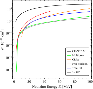
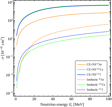
Figure 3: Top: elastic and NC inelastic $\nu$-⁴⁰Ar cross sections as a function of the incoming neutrino energy. For comparison our calculations (Multipole, Total GT and 1st GT) are compared with the CRPA [41] and free nucleon [43] predictions. Bottom: total elastic and NC inelastic neutrino-nucleus scattering cross sections for ⁴⁰Ar, ¹³³Cs, and ¹²⁷I nuclei.

In Fig. 3, we compare the inelastic cross section result of our two calculations, multipole and GT, with the CE$\nu$NS cross section and with two other inelastic results from the literature. While different calculations show some agreement at lower energies but diverge at higher energy. Our calculation of the total inelastic cross section (given as the sum over all GT transitions) is around an order of magnitude lower than that of Refs. [43] and more closely follows that of [41] until around $E_{\nu}=40$ MeV. The former used the free nucleon approximation to calculate just one excited state and so agreement is only expected for very small neutrino energies when few states are kinematically accessible. The latter calculates the inclusive inelastic cross section, above nucleon emission threshold, for low-lying states through the Continuum Random Phase Approximation (CRPA). Working with a limited spectrum of excited states, our multipole results can only include transitions to the first 15 excited states and thus it is unable to capture all accessible transitions and therefore is not an accurate estimate of the total cross section above $E_{\nu}\gtrsim 10$ MeV. However, we can use it to assess the contribution of non-GT transitions since the limited spectrum contains one $J=1$ state ($N=9$) that is accessible via a GT transition. For comparison we have plotted the GT cross section, Eq. (11), for the lowest lying $J=1$ state (gray curve in Fig. 3 top). This confirms that the GT transitions provide the dominant contribution to the inelastic cross section. Additionally we show the differential cross section as a function of angle and the recoil energy in appendix B.

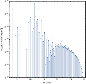
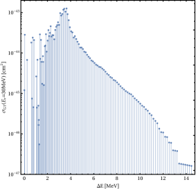
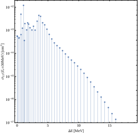
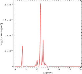
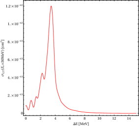
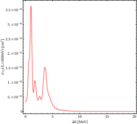
Figure 4: The GT transition cross section for each state vs. the excitation energy in ⁴⁰Ar (left), ¹³³Cs (center) and ¹²⁷I (right), for incident neutrinos with $E_{\nu}=30$ MeV. The top row shows the cross sections for each discrete energy level, while the bottom row shows these levels convolved with a Gaussian of width 150 keV.

Additional terms in the multipole expansion do contribute and are required for a precise calculation of the cross section for any specific transition. However, when estimating the total cross section, based on the limitations of our calculation, it is much more accurate to ensure that all accessible GT transitions are included. For the same number of states, the GT analysis generally consumes much less computational resources than the multipole analysis. For this reason and the aforementioned improvement in accuracy we use the GT analysis for our results in the following sections.

The total elastic and inelastic cross-sections for the ¹³³Cs and ¹²⁷I targets are shown in Fig. 3, where we have included GT transitions to 300 and 100 states (including the states with zero strength) for ¹³³Cs and ¹²⁷I, respectively. The elastic cross sections of both nuclei are virtually the same as they have a similar number of neutrons. In contrast, ¹²⁷I has slight higher inelastic cross section since it has a higher total GT strength than ¹³³Cs, as shown in Fig. 4.

Experimentally the signature of an inelastic collision will be dominated by the deexcitation energy of the nucleus. The excited nucleus falls back to the ground state very quickly through the emission of photons and (if energetically allowed) neutrons. Previous studies focused on the nuclear recoil energy, which is small in comparison, but could in principle be measured (recoil spectra are provided in appendix B). While a full calculation of the observational signatures is beyond the scope of this work, we can use the cross section to each excited state to visualize the relative strength of the energy depositions for each of the allowed transitions. In Fig. 4 we plot the cross section for each transition vs. the excitation energy for ⁴⁰Ar, ¹³³Cs and ¹²⁷I for a incoming neutrino energy of 30 MeV.

IV.3 DM-nucleus cross sections

Following the method of the previous section we computed the total cross section for dark matter inelastic scattering using the GT operator in the long wavelength limit. Similar to the neutrino case, we find that GT transitions also dominate the total cross section, as shown in Fig. 9

In Fig. 5, we show the elastic and inelastic cross section for dark matter scattering on the target nuclei ⁴⁰Ar, ¹³³Cs and ¹²⁷I assuming $m_{\chi}=30$ MeV, $m_{A^{\prime}}=90$ MeV, $\epsilon=10^{-4}$ and $g_{D}=\sqrt{2\pi}$ (this parameter space is allowed by the current experimental data [21]). Since the dark matter is not massless, $E_{\chi}$ has a threshold of 30 MeV, as shown in Fig. 6 and Fig. 5. The cross section $\sigma$ is proportional to the couplings constant $\epsilon^{2}$, so one can scale this plot by changing $\epsilon$. As expected we find that ¹³³Cs and ¹²⁷I have a higher elastic cross section than ⁴⁰Ar since $\sigma_{\rm el}$ has explicit $Z^{2}$ (atomic number) dependence, but have a lower inelastic cross section where $\sigma_{\rm inel}$ is determined by the GT strength, as shown in Fig. 4. The GT transition cross section is the largest for ⁴⁰Ar and is the lowest for ¹³³Cs. There is a plateau for $\chi-^{40}$Ar in Fig. 5, but not in ¹³³Cs or ¹²⁷I. This is because there are fewer low lying states in ⁴⁰Ar than ¹³³Cs or ¹²⁷I. We also observe a small plateau in $\nu-^{40}$Ar in Fig. 3, but this is not as noticeable as with DM scattering since the neutrino is massless. We also calculate the recoil energy spectrum for dark matter scattering in appendix B.

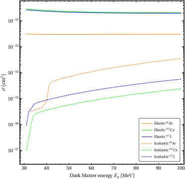
Figure 5: Total elastic and inelastic DM-nucleus scattering cross section for ⁴⁰Ar, ¹³³Cs, and ¹²⁷I nuclei with $m_{\chi}=30$ MeV.

V Scattering rates and experimental signatures

Table 1: Specifications of the experiments and detectors. Both experiments use a proton beam, and the POT values are expected spills for 5,000 hours of operation per year.

Experiment	$E_{\rm beam}$	POT	Target	Detector:
	[GeV]	[yr-1]		target	mass	distance	angle	$E_{r}^{\rm th}$
COHERENT	1	$1.5\times 10^{23}$	Hg	CsI[Na]	14.6 kg	19.3 m	90∘	6.5 keV
[1, 22, 83]				Ar	24.4 kg	28.4 m	137∘	20 keV
CCM [2, 24]	0.8	$1.0\times 10^{22}$	W	Ar	7 t	20 m	90∘	25 keV

Using the results of the previous section we compute the rates for neutrino and DM scattering off ⁴⁰Ar, ¹³³Cs, and ¹²⁷I nuclei. For a source of neutrinos or DM with flux $\Phi$ [cm^-2 s^-1], the number of events expected, $N$, is given by

$$N ={\mathrm{exposure}}\times\frac{1}{m_{T}}\times\Phi\int\sigma(E)\frac{dP}{dE}dE$$

where the exposure has dimensions of mass$\times$time, $m_{T}$ is the target mass, $E$ is the energy of incident particle ($\nu$ or DM) and $\frac{dP}{dE}$ is the corresponding normalized energy distribution (i.e. $\int\frac{dP}{dE}dE=1$). For neutrinos, we consider pion decay at rest sources, and for DM we simulate the energy spectra in both COHERENT and CCM. For the dark matter spectrum we need to determine the production rates of relevant mesons. We use the results from Ref. [46] which uses GEANT4 to determine these production rates at CCM and COHERENT. In addition to $\pi^{0}$ decays and $\pi^{-}$ absorption, $e^{\pm}$ induced cascades photons are important to produce dark photons for the DM production. We show the DM energy spectrum for CCM (which uses an 800 MeV proton beam), along with the neutrino energy spectra at COHERENT (which uses a 1 GeV proton beam) in Fig. 6 with $m_{\chi}=30$ MeV.

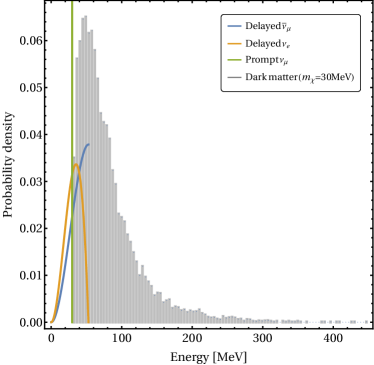
Figure 6: Energy spectra of $\pi$-DAR neutrinos and a sample DM spectrum (in CCM) assuming $m_{A^{\prime}}=3m_{\chi}=90$ MeV.

Table 1 summarizes the key specifications of the experiments we consider, we additionally assume a detection efficiency of 100% and that all energy depositions are above threshold. As an example we take the DM mass to be $m_{\chi}=30$ MeV, dark photon mass $m_{A^{\prime}}=90$ MeV with coupling constants $\epsilon=10^{-4}$ and $g_{D}=\sqrt{2\pi}$. We assume that CCM will operate continuously for 3 years with $3\times 10^{22}$ POT, while COHERENT has already ran for $\sim 1.61$ years with their CsI detector ($m_{T}=14.6$ kg) with $3.20\times 10^{23}$ POT and approximately 0.6 years with their LAr detector ($m_{T}=24.4$ kg) with $1.34\times 10^{23}$ POT. Table 2 shows the estimated number of events for the two experiments under these assumptions. The DM energy spectrum has a broader energy range extending up to hundreds of MeV, much higher than the neutrino spectrum. The high energy tail causes DM to induce a higher rate of inelastic events compared to neutrinos. Therefore, the elastic to inelastic event ratios for DM are lower in all detectors.

Table 2: Number of elastic and NC inelastic neutrino-nucleus, and elastic and inelastic DM-nucleus scattering events ($m_{\chi}=30$ MeV) for different experimental configurations given in table 1.

Scattering	Experiment	Elastic	Inelastic	Ratio
$\nu$-40Ar	COHERENT	$2.27\times 10^{2}$	$3.15$	$7.21\times 10$
$\nu$-40Ar	CCM	$1.91\times 10^{4}$	$2.65\times 10^{2}$	$7.21\times 10$
$\nu$-133Cs	COHERENT	$1.16\times 10^{3}$	$1.52\times 10^{-2}$	$7.65\times 10^{3}$
$\nu$-127I	COHERENT	$1.06\times 10^{3}$	$3.75\times 10^{-1}$	$2.81\times 10^{3}$
$\chi$-40Ar	COHERENT	$1.18$	$1.13\times 10^{-1}$	$1.04\times 10$
$\chi$-40Ar	CCM	$9.92\times 10$	$9.52$	$1.04\times 10$
$\chi$-133Cs	COHERENT	$4.11$	$4.91\times 10^{-3}$	$8.38\times 10^{2}$
$\chi$-127I	COHERENT	$3.87$	$1.16\times 10^{-2}$	$3.33\times 10^{2}$

VI Conclusion

We have applied the nuclear shell model to calculate cross sections of neutrino-nucleus and DM-nucleus scattering. The DM particles are produced from the light vector mediator and this mediator is produced from the kinetic mixing with photons in the stopped-pion experiments (with $\sim 1$ GeV proton beam) we are considering. The number of states we calculated is large enough to include all non-trivial contributions such that the outcome is reliable. In particular we focus on argon, caesium, and iodine nuclei. We computed the cross section in two formalisms: a multipole analysis and the Gamow–Teller operator alone in the long-wavelength limit. We found that Gamow–Teller transitions dominate all other transitions for both neutrino and DM inelastic scattering. Using the Gamow-Teller operator, our calculations show that the inelastic cross section is a few orders of magnitude smaller than the elastic cross section for both neutrino and dark matter scattering. We also computed rates for two experimental setups based on the computed cross section. The inelastic scattering rate is much smaller than the elastic rate, but it will produce a much larger energy deposition that is potentially easier to observe. In the setup we consider, since dark matter spectrum has a higher energy tail than neutrinos, the inelastic contribution is higher and the ratio of the inelastic to the elastic rate can be as large as 0.1 for argon targets. The inelastic neutrino and DM scattering results presented here can be measured in currently running stopped-pion experiments, such as at CCM and COHERENT, and provide additional channels to explore beyond the elastic scattering channel for which they were initially conceived.

Appendix A DM current derivation

Some useful kinematics identities

$$\cos\theta = {\vec{p_{i}}^{2}+\vec{p_{f}}^{2}-2ME_{r}\over 2\,p_{i}\,p_{f}}$$ (23)

$$\vec{p_{i}}\cdot\vec{p_{f}} = {1\over 2}(\vec{p_{i}}^{2}+\vec{p_{f}}^{2}-2ME_{r})$$ (24)

where $\vec{p_{i}}/\vec{p_{f}}$ is the incoming/outgoing DM momentum, $M$ is the nucleus mass and $E_{r}$ is the nuclear recoil energy. In the follows we derive the DM currents of Eq. (17) in more detail, the DM mass is taken to be $m$:

$$\sum\limits_{s_{i},s_{f}}l_{\mu}l_{\nu}^{*} =Tr\left(\frac{\cancel{p_{f}}+m}{2E_{f}}\,\gamma^{\mu}\,\frac{\cancel{p_{i}}+m}{2E_{i}}\gamma^{\nu}\right)$$

$$=\frac{1}{4E_{f}E_{i}}\left[Tr\left(\cancel{p_{f}}\,\gamma^{\mu}\,\cancel{p_{i}}\,\gamma^{\nu}+m^{2}\gamma^{\mu}\gamma^{\nu}\right)\right]$$

where $Tr$ means trace of the matrix. Insert numbers to $\mu$ and $\nu$,

$$\sum\limits_{s_{i},s_{f}}l_{0}l_{0}^{*} =\frac{1}{4E_{f}E_{i}}\left[Tr\left(p_{f}^{\alpha}\,\gamma^{\alpha}\,\gamma^{0}\,p_{i}^{\beta}\,\gamma^{\beta}\,\gamma^{0}+m^{2}\gamma^{0}\gamma^{0}\right)\right]$$

$$=\frac{1}{4E_{i}E_{f}}\left[4p_{f}^{\alpha}p_{i}^{\beta}(g^{\alpha 0}g^{\beta 0}-g^{\alpha\beta}g^{00}+g^{\alpha 0}g^{\beta 0})+m^{2}g^{00}\right]$$

$$=\frac{1}{E_{i}E_{f}}\left(2p_{f}^{0}p_{i}^{0}-p_{i}\cdot p_{f}+\frac{m^{2}}{4}\right)$$

$$=\frac{1}{E_{i}E_{f}}\left(p_{f}^{0}p_{i}^{0}+\vec{p_{i}}\cdot\vec{p_{f}}+\frac{m^{2}}{4}\right)$$

$$=1+\frac{\vec{p_{i}}\cdot\vec{p_{f}}}{E_{i}E_{f}}+\frac{m^{2}}{4E_{i}E_{f}}$$

$$=1+\frac{\vec{p_{i}}^{2}+\vec{p_{f}}^{2}-2ME_{r}}{2E_{i}E_{f}}+\frac{m^{2}}{4E_{i}E_{f}}$$

$$=1+\frac{1}{4E_{i}E_{f}}\left(2\vec{p_{i}}^{2}+2\vec{p_{f}}^{2}-4ME_{r}+m^{2}\right)$$

$$\sum\limits_{s_{i},s_{f}}l_{3}l_{3}^{*} =\frac{1}{4E_{f}E_{i}}\left[Tr\left(p_{f}^{\alpha}\,\gamma^{\alpha}\,\gamma^{3}\,p_{i}^{\beta}\,\gamma^{\beta}\,\gamma^{3}+m^{2}\gamma^{3}\gamma^{3}\right)\right]$$

$$=\frac{1}{E_{i}E_{f}}\left(-2p_{f}^{3}p_{i}^{3}+p_{i}\cdot p_{f}-\frac{m^{2}}{4}\right)$$

$$=\frac{1}{E_{i}E_{f}}\Big{[}-2p_{i}p_{f}\cos\theta+\Big{(}E_{i}E_{f}-{1\over 2}(\vec{p_{i}}^{2}$$

$$+\vec{p_{f}}^{2}-2ME_{r})\Big{)}-{m^{2}\over 4}\Big{]}$$

$$=1+\frac{1}{E_{i}E_{f}}\left[-{3\over 2}\left(\vec{p_{i}}^{2}+\vec{p_{f}}^{2}\right)+3ME_{r}-{m^{2}\over 4}\right]$$

$$\sum\limits_{s_{i},s_{f}}l_{3}l_{0}^{*} =\frac{1}{4E_{f}E_{i}}\left[Tr\left(p_{f}^{\alpha}\,\gamma^{\alpha}\,\gamma^{3}\,p_{i}^{\beta}\,\gamma^{\beta}\,\gamma^{0}+m^{2}\gamma^{3}\gamma^{0}\right)\right]$$

$$=\frac{p_{f}^{\alpha}p_{i}^{\beta}}{E_{i}E_{f}}\left(g^{\alpha 3}g^{\beta 0}-g^{\alpha\beta}g^{30}+g^{\alpha 0}g^{3\beta}\right)$$

$$=-\frac{1}{E_{i}E_{f}}\left(p_{f}^{3}p_{i}^{0}+p_{f}^{0}p_{i}^{3}\right)$$

$$=-\left(\frac{p_{f}^{3}}{E_{f}}+\frac{p_{i}^{3}}{E_{i}}\right)$$

$$=-\left({\vec{p_{i}}^{2}+\vec{p_{f}}^{2}-2ME_{r}\over 2p_{i}E_{f}}+{p_{i}\over E_{i}}\right)$$

Summing over $k=1,2,3$

$$\sum\limits_{s_{i},s_{f}}l_{k}l_{k}^{*} =\frac{1}{4E_{f}E_{i}}\left[Tr\left(p_{f}^{\alpha}\,\gamma^{\alpha}\,\gamma^{k}\,p_{i}^{\beta}\,\gamma^{\beta}\,\gamma^{k}+m^{2}\gamma^{k}\gamma^{k}\right)\right]$$

$$=\frac{1}{E_{i}E_{f}}\left[p_{f}^{\alpha}p_{i}^{\beta}\left(g^{\alpha k}g^{\beta k}-g^{\alpha\beta}g^{kk}+g^{\alpha k}g^{\beta k}\right)+\frac{m^{2}}{4}g^{kk}\right]$$

$$=\frac{1}{E_{i}E_{f}}\left[p_{f}^{\alpha}p_{i}^{\beta}\left(2g^{\alpha k}g^{\beta k}+3g^{\alpha\beta}\right)-\frac{3}{4}m^{2}\right]$$

$$=\frac{1}{E_{i}E_{f}}\left(3E_{i}E_{f}-\vec{p_{i}}\cdot\vec{p_{f}}-\frac{3}{4}m^{2}\right)$$

$$=3-{1\over E_{i}E_{f}}\left[{1\over 2}\left(\vec{p_{i}}^{2}+\vec{p_{f}}^{2}-2ME_{r}\right)+{3m^{2}\over 4}\right]$$

$$\sum\limits_{s_{i},s_{f}} (\vec{l}\times\vec{l}^{*})_{3}=\sum\limits_{s_{i},s_{f}}l_{1}l_{2}^{*}-\sum\limits_{s_{i},s_{f}}l_{2}l_{1}^{*}$$

$$=\frac{1}{4E_{i}E_{f}}\left[Tr\left(p_{f}^{\alpha}\gamma^{\alpha}\gamma^{1}p_{i}^{\beta}\gamma^{\beta}\gamma^{2}\right)-Tr\left(p_{f}^{\alpha}\gamma^{\alpha}\gamma^{2}p_{i}^{\beta}\gamma^{\beta}\gamma^{1}\right)\right]$$

$$=\frac{p_{f}^{\alpha}p_{i}^{\beta}}{E_{i}E_{f}}[(g^{\alpha 1}g^{\beta 2}-g^{\alpha\beta}g^{12}+g^{\alpha 2}g^{1\beta})$$

$$-(g^{\alpha 2}g^{\beta 1}-g^{\alpha\beta}g^{12}+g^{\alpha 1}g^{2\beta})]$$

$$=0$$

Appendix B Shell model results

For a more detailed comparison in Fig. 7 we show the differential neutrino-nucleus cross section as a function of $\cos{\theta}$ for the multipole analysis (including the first 15 transitions) and the GT analysis involving the first transition for a given incoming neutrino energy $E_{\nu}=30$ MeV. Again we see that the $N=9$ transition, the lowest lying GT transition, dominates the inelastic cross section. Fig. 8 shows Gamow-Teller cross section in recoil energy $E_{r}$.

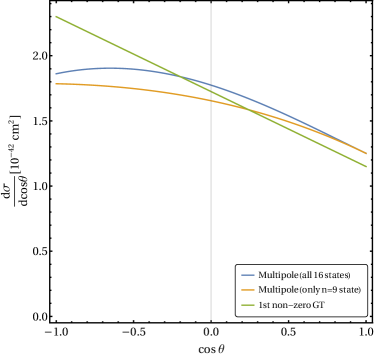
Figure 7: The differential cross section as a function of scattering angle, for NC inelastic $\nu$-⁴⁰Ar scattering with $E_{\nu}=30$ MeV. The blue and orange curves are calculated using the full cross section formula Eq. (2), while the green curve is calculated in the long wavelength limit using Eq. (10).

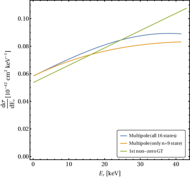
Figure 8: Similar to Fig. 7, but differential cross section $\frac{d\sigma}{dE_{r}}$ plotted as a function of recoil energy $E_{r}$.

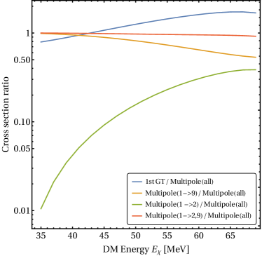
Figure 9: Multipole and GT cross section ratios of $\chi-^{40}$Ar scattering with $m_{\chi}=30$ MeV.

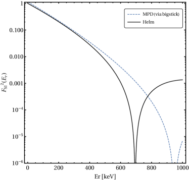
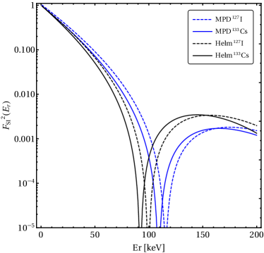
Figure 10: Elastic scattering form factors: the Helm parametrization compared with the ground state to ground state transition found via our shell model calculation for ⁴⁰Ar (left) and ¹³³Cs and ¹²⁷I (right).

Fig. 9 shows multipoles and GT ratios of $\chi-^{40}$Ar scattering cross section. In which Multipole (all) is the sum of all the transitions $1\rightarrow 2..16$, dominated by $1\rightarrow 2$ and $1\rightarrow 9$ transitions. Similar to neutrino case, sum of all the multipole is roughly equivalent to the first GT transition ($1\rightarrow 9$). Nevertheless, both $\nu$ and DM match better in low $E_{r}$/$E_{\chi}$, while they become less consistent with the long-wave length limit in the relatively higher $E_{r}$/$E_{\chi}$ due to the kinematics.

In Fig. 10 we plot the shell model ground state to ground state transition compared to the Helm form factor to benchmark the shell-model accuracy and consistency. The difference between our multipole decomposition (MPD) and the Helm form factors is greater than that obtained for the Xe nucleus in [49] where the GCN5082 interaction was used (note their form factors are plotted as functions of dimensionless $u\equiv q^{2}b^{2}/2$ instead of $E_{r}$ in Fig. 10). The harmonic oscillator parameter is taken to be $b=\sqrt{41.467/(45A^{-1/3}-25A^{-2/3})}\mathrm{fm}$, which is $\sim 2.3$fm for Cs and I. We note that the agreement is good at low momentum transfer, which is most relevant to this work. That said, investigating this discrepancy is a potential line for future work.

Table 3: Nuclear magnetic moments $\mu$ (nm), energy level $E_{x}$ [keV] and $J^{\pi}$ spin partiy for the nuclear states of ⁴⁰Ar, ¹²⁷I, and ¹³³Cs. Here we label the excited states with $i$, where $i=1$ is the ground state.

Nucleus	$i$	$J^{\pi}$	Expt.	$\mu$	Expt.	$E_{x}$	Expt.
127I	1	$5/2^{+}$	$5/2^{+}$	3.851	2.813	0	0
	2	$7/2^{+}$	$7/2^{+}$	3.007	2.54	37.44	57.61
	3	$3/2^{+}$	$3/2^{+}$	0.9155	0.97	285.9	202.86
133Cs	1	$7/2^{+}$	$7/2^{+}$	3.007	2.582	0	0
	2	$5/2^{+}$	$5/2^{+}$	3.851	3.45	36.37	80.9979
	3	$5/2^{+}$	$5/2^{+}$	2.5849	2.0	235.36	160.6101
40Ar	1	$0^{+}$	$0^{+}$	0		0	0
	2	$2^{+}$	$2^{+}$	0	-0.04	1118.33	1460.85
	3	$2^{+}$	$0^{+}$			2054.05	2120.83
	4	$4^{+}$	$2^{+}$			2346.64	2524.12
	5	$0^{+}$	$4^{+}$			2485.19	2892.61

Figure 11: Energy levels and spins of ⁴⁰Ar

Figure 12: Energy levels and spins of ¹³³Cs and ¹²⁷I

Table 3 gives the nuclear magnetic moments $\mu$ (nm) and excitation energies $E_{x}$ (keV) of the first few states from our shell model calculation, which compare reasonably well with the experimental values [42, 84]. Our shell model predicts that the first excited state of ⁴⁰Ar has 2 protons moved from 0d_3/2 (ground state) to 0f_7/2, so every nucleon is paired, which implies $\mu=0$.

References

- [1] COHERENT Collaboration, D. Akimov et al., Observation of Coherent Elastic Neutrino-Nucleus Scattering, Science 357 (2017) 1123 [1708.01294].
- [2] R. van de Water and Coherent-Mills Experiment Team, Searching for Sterile Neutrinos with the Coherent CAPTAIN-Mills Detector at the Los Alamos Neutron Science Center, in APS April Meeting Abstracts, vol. 2019 of APS Meeting Abstracts, p. Z14.009, Jan., 2019.
- [3] D. Akimov et al., Measurement of the Coherent Elastic Neutrino-Nucleus Scattering Cross Section on CsI by COHERENT, 2110.07730.
- [4] T. Ohlsson, Status of non-standard neutrino interactions, Rept. Prog. Phys. 76 (2013) 044201 [1209.2710].
- [5] O. G. Miranda and H. Nunokawa, Non standard neutrino interactions: current status and future prospects, New J. Phys. 17 (2015) 095002 [1505.06254].
- [6] J. B. Dent, B. Dutta, S. Liao, J. L. Newstead, L. E. Strigari and J. W. Walker, Accelerator and reactor complementarity in coherent neutrino-nucleus scattering, Phys. Rev. D 97 (2018) 035009 [1711.03521].
- [7] J. Liao and D. Marfatia, COHERENT constraints on nonstandard neutrino interactions, Phys. Lett. B 775 (2017) 54 [1708.04255].
- [8] P. B. Denton, Y. Farzan and I. M. Shoemaker, Testing large non-standard neutrino interactions with arbitrary mediator mass after COHERENT data, JHEP 07 (2018) 037 [1804.03660].
- [9] J. Billard, J. Johnston and B. J. Kavanagh, Prospects for exploring New Physics in Coherent Elastic Neutrino-Nucleus Scattering, JCAP 11 (2018) 016 [1805.01798].
- [10] W. Altmannshofer, M. Tammaro and J. Zupan, Non-standard neutrino interactions and low energy experiments, JHEP 09 (2019) 083 [1812.02778]. [Erratum: JHEP 11, 113 (2021)].
- [11] B. Dutta, S. Liao, S. Sinha and L. E. Strigari, Searching for Beyond the Standard Model Physics with COHERENT Energy and Timing Data, Phys. Rev. Lett. 123 (2019) 061801 [1903.10666].
- [12] B. C. Canas, E. A. Garces, O. G. Miranda, A. Parada and G. Sanchez Garcia, Interplay between nonstandard and nuclear constraints in coherent elastic neutrino-nucleus scattering experiments, Phys. Rev. D 101 (2020) 035012 [1911.09831].
- [13] A. N. Khan and W. Rodejohann, New physics from COHERENT data with an improved quenching factor, Phys. Rev. D 100 (2019) 113003 [1907.12444].
- [14] P. Coloma, I. Esteban, M. C. Gonzalez-Garcia and J. Menendez, Determining the nuclear neutron distribution from Coherent Elastic neutrino-Nucleus Scattering: current results and future prospects, JHEP 08 (2020) 030 [2006.08624].
- [15] P. B. Denton and J. Gehrlein, A Statistical Analysis of the COHERENT Data and Applications to New Physics, JHEP 04 (2021) 266 [2008.06062].
- [16] B. Dutta, R. F. Lang, S. Liao, S. Sinha, L. Strigari and A. Thompson, A global analysis strategy to resolve neutrino NSI degeneracies with scattering and oscillation data, JHEP 09 (2020) 106 [2002.03066].
- [17] P. deNiverville, M. Pospelov and A. Ritz, Observing a light dark matter beam with neutrino experiments, Phys. Rev. D 84 (2011) 075020 [1107.4580].
- [18] P. deNiverville, M. Pospelov and A. Ritz, Light new physics in coherent neutrino-nucleus scattering experiments, Phys. Rev. D92 (2015) 095005 [1505.07805].
- [19] S.-F. Ge and I. M. Shoemaker, Constraining Photon Portal Dark Matter with Texono and Coherent Data, JHEP 11 (2018) 066 [1710.10889].
- [20] B. Dutta, D. Kim, S. Liao, J.-C. Park, S. Shin and L. E. Strigari, Dark matter signals from timing spectra at neutrino experiments, Phys. Rev. Lett. 124 (2020) 121802.
- [21] COHERENT Collaboration, D. Akimov et al., First Probe of Sub-GeV Dark Matter Beyond the Cosmological Expectation with the COHERENT CsI Detector at the SNS, 2110.11453.
- [22] COHERENT Collaboration, D. Akimov et al., Sensitivity of the COHERENT Experiment to Accelerator-Produced Dark Matter, Phys. Rev. D 102 (2020) 052007 [1911.06422].
- [23] A. A. Aguilar-Arevalo et al., First Leptophobic Dark Matter Search from Coherent CAPTAIN-Mills, 2109.14146.
- [24] CCM Collaboration, A. A. Aguilar-Arevalo et al., First Dark Matter Search Results From Coherent CAPTAIN-Mills, 2105.14020.
- [25] DUNE Collaboration, B. Abi et al., Supernova neutrino burst detection with the Deep Underground Neutrino Experiment, Eur. Phys. J. C 81 (2021) 423 [2008.06647].
- [26] Hyper-Kamiokande Collaboration, K. Abe et al., Physics potentials with the second Hyper-Kamiokande detector in Korea, PTEP 2018 (2018) 063C01 [1611.06118].
- [27] KARMEN Collaboration, R. Maschuw, Neutrino spectroscopy with KARMEN, Prog. Part. Nucl. Phys. 40 (1998) 183.
- [28] LSND Collaboration, L. B. Auerbach et al., Measurements of charged current reactions of nu(e) on 12-C, Phys. Rev. C 64 (2001) 065501 [hep-ex/0105068].
- [29] W. C. Haxton, The Nuclear Response of Water Cherenkov Detectors to Supernova and Solar Neutrinos, Phys. Rev. D 36 (1987) 2283.
- [30] E. Kolbe, K. Langanke, S. Krewald and F. K. Thielemann, Inelastic neutrino scattering on C-12 and O-16 above the particle emission threshold, Nucl. Phys. A 540 (1992) 599.
- [31] W. E. Ormand, P. M. Pizzochero, P. F. Bortignon and R. A. Broglia, Neutrino capture cross-sections for Ar-40 and Beta decay of Ti-40, Phys. Lett. B 345 (1995) 343 [nucl-th/9405007].
- [32] E. Kolbe, K. Langanke and G. Martinez-Pinedo, The Inclusive Fe-56 (electron neutrino, e-) Co-56 cross-section, Phys. Rev. C 60 (1999) 052801 [nucl-th/9905001].
- [33] A. C. Hayes and I. S. Towner, Shell model calculations of neutrino scattering from C-12, Phys. Rev. C 61 (2000) 044603 [nucl-th/9907049].
- [34] C. Volpe, N. Auerbach, G. Colo, T. Suzuki and N. Van Giai, Microscopic theories of neutrino C-12 reactions, Phys. Rev. C 62 (2000) 015501 [nucl-th/0001050].
- [35] J. Engel, G. C. McLaughlin and C. Volpe, What can be learned with a lead based supernova neutrino detector?, Phys. Rev. D 67 (2003) 013005 [hep-ph/0209267].
- [36] T. Suzuki, S. Chiba, T. Yoshida, T. Kajino and T. Otsuka, Neutrino nucleus reactions based on new shell model Hamiltonians, Phys. Rev. C 74 (2006) 034307 [nucl-th/0608056].
- [37] T. Suzuki, M. Honma, K. Higashiyama, T. Yoshida, T. Kajino, T. Otsuka, H. Umeda and K. Nomoto, Neutrino-induced reactions on Fe-56 and Ni-56, and production of Mn-55 in population III stars, Phys. Rev. C 79 (2009) 061603.
- [38] M.-K. Cheoun, E. Ha, T. Hayakawa, S. Chiba, K. Nakamura, T. Kajino and G. J. Mathews, Neutrino induced reactions related to the -process nucleosynthesis of 92Nb and 98Tc, Phys. Rev. C 85 (2012) 065807 [1108.4229].
- [39] J. Kostensalo, J. Suhonen and K. Zuber, Shell-model computed cross sections for charged-current scattering of astrophysical neutrinos off 40Ar, Phys. Rev. C 97 (2018) 034309.
- [40] N. Van Dessel, N. Jachowicz and A. Nikolakopoulos, Forbidden transitions in neutral and charged current interactions between low-energy neutrinos and Argon, Phys. Rev. C 100 (2019) 055503 [1903.07726].
- [41] N. Van Dessel, V. Pandey, H. Ray and N. Jachowicz, Nuclear Structure Physics in Coherent Elastic Neutrino-Nucleus Scattering, 2007.03658.
- [42] R. Sahu, D. K. Papoulias, V. K. B. Kota and T. S. Kosmas, Elastic and inelastic scattering of neutrinos and weakly interacting massive particles on nuclei, Phys. Rev. C 102 (2020) 035501 [2004.04055].
- [43] V. A. Bednyakov and D. V. Naumov, Coherency and incoherency in neutrino-nucleus elastic and inelastic scattering, Phys. Rev. D 98 (2018) 053004.
- [44] A. Nikolakopoulos, V. Pandey, J. Spitz and N. Jachowicz, Modeling quasielastic interactions of monoenergetic kaon decay-at-rest neutrinos, Phys. Rev. C 103 (2021) 064603 [2010.05794].
- [45] V. Pandey, N. Jachowicz, T. Van Cuyck, J. Ryckebusch and M. Martini, Low-energy excitations and quasielastic contribution to electron-nucleus and neutrino-nucleus scattering in the continuum random-phase approximation, Phys. Rev. C 92 (2015) 024606 [1412.4624].
- [46] B. Dutta, D. Kim, S. Liao, J.-C. Park, S. Shin, L. E. Strigari and A. Thompson, Searching for dark matter signals in timing spectra at neutrino experiments, JHEP 01 (2022) 144 [2006.09386].
- [47] B. Dutta, D. Kim, A. Thompson, R. T. Thornton and R. G. Van de Water, Solutions to the MiniBooNE Anomaly from New Physics in Charged Meson Decays, 2110.11944.
- [48] L. Baudis, G. Kessler, P. Klos, R. F. Lang, J. Menéndez, S. Reichard and A. Schwenk, Signatures of Dark Matter Scattering Inelastically Off Nuclei, Phys. Rev. D 88 (2013) 115014 [1309.0825].
- [49] L. Vietze, P. Klos, J. Menéndez, W. C. Haxton and A. Schwenk, Nuclear structure aspects of spin-independent WIMP scattering off xenon, Phys. Rev. D 91 (2015) 043520 [1412.6091].
- [50] R. H. Helm, Inelastic and Elastic Scattering of 187-Mev Electrons from Selected Even-Even Nuclei, Phys. Rev. 104 (1956) 1466.
- [51] M. Hoferichter, J. Menéndez and A. Schwenk, Coherent elastic neutrino-nucleus scattering: EFT analysis and nuclear responses, Phys. Rev. D 102 (2020) 074018 [2007.08529].
- [52] O. Tomalak, P. Machado, V. Pandey and R. Plestid, Flavor-dependent radiative corrections in coherent elastic neutrino-nucleus scattering, JHEP 02 (2021) 097 [2011.05960].
- [53] T. De Forest, Jr. and J. D. Walecka, Electron scattering and nuclear structure, Adv. Phys. 15 (1966) 1.
- [54] B. D. Serot, Semileptonic Weak and Electromagnetic Interactions with Nuclei: Nuclear Current Operators Through Order (v/c)**2 (Nucleon), Nucl. Phys. A 308 (1978) 457.
- [55] T. W. Donnelly and W. C. Haxton, Multipole operators in semileptonic weak and electromagnetic interactions with nuclei, Atom. Data Nucl. Data Tabl. 23 (1979) 103.
- [56] J. Walecka, Theoretical Nuclear and Subnuclear Physics, Theoretical Nuclear and Subnuclear Physics. Imperial College Press, 2004.
- [57] W. Haxton and C. Lunardini, A Mathematica script for harmonic oscillator nuclear matrix elements arising in semileptonic electroweak interactions, Comput. Phys. Commun. 179 (2008) 345 [0706.2210].
- [58] V. Bernard, L. Elouadrhiri and U.-G. Meißner, Axial structure of the nucleon, Journal of Physics G: Nuclear and Particle Physics 28 (2001) R1.
- [59] T. W. Donnelly and W. C. Haxton, Multipole operators in semileptonic weak and electromagnetic interactions with nuclei, Atom. Data Nucl. Data Tabl. 25 (1980) 1.
- [60] V. Tsakstara and T. Kosmas, Nuclear responses to astrophysical neutrinos through the neutral gamow-teller strength, HNPS Advances in Nuclear Physics 20 (2012) 96.
- [61] S. Gardiner, Nuclear de-excitations in low-energy charged-current scattering on , Phys. Rev. C 103 (2021) 044604.
- [62] P. Klos, J. Menéndez, D. Gazit and A. Schwenk, Large-scale nuclear structure calculations for spin-dependent wimp scattering with chiral effective field theory currents, Phys. Rev. D 88 (2013) 083516.
- [63] G. Arcadi, C. Döring, C. Hasterok and S. Vogl, Inelastic dark matter nucleus scattering, JCAP 12 (2019) 053 [1906.10466].
- [64] J.-H. Huh, J. E. Kim, J.-C. Park and S. C. Park, Galactic 511 keV line from MeV milli-charged dark matter, Phys. Rev. D77 (2008) 123503 [0711.3528].
- [65] M. Pospelov, A. Ritz and M. B. Voloshin, Secluded WIMP Dark Matter, Phys. Lett. B662 (2008) 53 [0711.4866].
- [66] E. J. Chun, J.-C. Park and S. Scopel, Dark matter and a new gauge boson through kinetic mixing, JHEP 02 (2011) 100 [1011.3300].
- [67] B. Batell, P. deNiverville, D. McKeen, M. Pospelov and A. Ritz, Leptophobic Dark Matter at Neutrino Factories, Phys. Rev. D 90 (2014) 115014 [1405.7049].
- [68] D. E. Kaplan, M. A. Luty and K. M. Zurek, Asymmetric Dark Matter, Phys. Rev. D 79 (2009) 115016 [0901.4117].
- [69] X.-J. Bi, X.-G. He and Q. Yuan, Parameters in a class of leptophilic models from PAMELA, ATIC and FERMI, Phys. Lett. B 678 (2009) 168 [0903.0122].
- [70] J.-C. Park, J. Kim and S. C. Park, Galactic center GeV gamma-ray excess from dark matter with gauged lepton numbers, Phys. Lett. B 752 (2016) 59 [1505.04620].
- [71] P. Foldenauer, Light dark matter in a gauged model, Phys. Rev. D 99 (2019) 035007 [1808.03647].
- [72] B. Dutta, S. Ghosh and J. Kumar, A sub-GeV dark matter model, 1905.02692.
- [73] B. Dutta, D. Kim, S. Liao, J.-C. Park, S. Shin and L. E. Strigari, Dark matter signals from timing spectra at neutrino experiments, Phys. Rev. Lett. 124 (2020) 121802.
- [74] C. W. Johnson, W. E. Ormand, K. S. McElvain and H. Shan, BIGSTICK: A flexible configuration-interaction shell-model code, 1801.08432.
- [75] C. W. Johnson, W. E. Ormand and P. G. Krastev, Factorization in large-scale many-body calculations, Comput. Phys. Commun. 184 (2013) 2761 [1303.0905].
- [76] E. Caurier, G. Martinez-Pinedo, F. Nowacki, A. Poves and A. P. Zuker, The shell model as a unified view of nuclear structure, Reviews of Modern Physics 77 (2005) 427.
- [77] S. Bloom, Gamow-teller strength functions with the lanczos algorithm, Progress in Particle and Nuclear Physics 11 (1984) 505.
- [78] S. D. Bloom and G. M. Fuller, Gamow-Teller electron capture strength distributions in stars: Unblocked iron and nickel isotopes, Nucl. Phys. A. 440 (1985) 511.
- [79] B. A. Brown, N. J. Stone, J. R. Stone, I. S. Towner and M. Hjorth-Jensen, Magnetic moments of the states around , Phys. Rev. C 71 (2005) 044317.
- [80] F. M. Prados Estévez, A. M. Bruce, M. J. Taylor, H. Amro, C. W. Beausang, R. F. Casten, J. J. Ressler, C. J. Barton, C. Chandler and G. Hammond, Isospin purity of states in the nuclei studied via lifetime measurements in , Phys. Rev. C 75 (2007) 014309.
- [81] F. Nowacki and A. Poves, New effective interaction for shell-model calculations in the valence space, Phys. Rev. C 79 (2009) 014310.
- [82] S. Nummela, P. Baumann, E. Caurier, P. Dessagne, A. Jokinen, A. Knipper, G. Le Scornet, C. Miehé, F. Nowacki, M. Oinonen, Z. Radivojevic, M. Ramdhane, G. Walter and J. Äystö, Spectroscopy of by decay: shell gap and single-particle states, Phys. Rev. C 63 (2001) 044316.
- [83] D. Akimov et al., Coherent 2018 at the spallation neutron source, 2018. 10.48550/ARXIV.1803.09183.
- [84] Live chart of nuclides. nuclear structure and decay data, 2022. https://www-nds.iaea.org/relnsd/vcharthtml/VChartHTML.html.