DFG-NAS: Deep and Flexible Graph Neural Architecture Search

Abstract

Graph neural networks (GNNs) have been intensively applied to various graph-based applications. Despite their success, manually designing the well-behaved GNNs requires immense human expertise. And thus it is inefficient to discover the potentially optimal data-specific GNN architecture. This paper proposes DFG-NAS, a new neural architecture search (NAS) method that enables the automatic search of very deep and flexible GNN architectures. Unlike most existing methods that focus on micro-architectures, DFG-NAS highlights another level of design: the search for macro-architectures on how atomic propagation (P) and transformation (T) operations are integrated and organized into a GNN. To this end, DFG-NAS proposes a novel search space for P-T permutations and combinations based on message-passing dis-aggregation, defines four custom-designed macro-architecture mutations, and employs the evolutionary algorithm to conduct an efficient and effective search. Empirical studies on four node classification tasks demonstrate that DFG-NAS outperforms state-of-the-art manual designs and NAS methods of GNNs.

1 Introduction

Graph Neural Networks (GNNs) are a set of message passing algorithms, whose intuition is to smooth the node embedding across the edges of a graph. By staking multiple GNN layers, each node can enhance its node embedding with distant neighborhood nodes. Recently, GNNs have been applied in various domains such as social network analysis (Zhang et al., 2020; Huang et al., 2021), chemistry and biology (Dai et al., 2019; Bradshaw et al., 2019), recommendation (Jiang et al., 2022; Wu et al., 2020), natural language processing (Wu et al., 2021; Vashishth et al., 2020), and computer vision (Shi et al., 2019; Sarlin et al., 2020). Despite a broad spectrum of applications, designing GNN architectures manually is a knowledge-intensive and labor-intensive process. Existing literature (Huan et al., 2021) suggests that handcrafted architectures (e.g., GCN (Kipf & Welling, 2017), GraphSAGE (Hamilton et al., 2017), and GAT (Velickovic et al., 2018)) can not behave well in all scenarios. Therefore, there is an ever-increasing demand for automated architecture exploration to obtain the optimal data-specific GNN architectures.

Motivated by the success of neural architecture search (NAS) in other established areas, e.g., computer vision, several recent graph neural architecture search (G-NAS) methods are proposed to effectively tackle the architecture challenge in GNNs, including GraphNAS (Gao et al., 2020a), Auto-GNN (Zhou et al., 2019), and GraphGym (You et al., 2020). These G-NAS methods assume GNNs consist of several repetitive message passing layers, and focus more on the intra-layer design such as aggregation function and nonlinear activation function. Despite their effectiveness, they suffer from two limitations:

Fixed Pipeline Pattern. To generate GNNs, existing methods adopt a fixed message-passing pipeline to organize two types of atomic operations: propagating (P) representations of its neighbors and applying transformation (T) on the representations. In particular, most G-NAS methods adopt the tight entanglement of applying transformation after propagation in each layer (e.g., P-T-P-T). Several handcrafted architectures include a certain degree of entanglement by only retaining the first transformation or propagation, e.g., T-P-P-P (Klicpera et al., 2019; Liu et al., 2020) or P-P-P-T  (Wu et al., 2019; Rossi et al., 2020; Zhang et al., 2021c). However, these specific P-T permutations and combinations are still fixed pipeline designs, limiting the expressive power of macro-architecture search space. It remains to be seen whether more general and flexible pipelines can further improve the performance.

Restricted Pipeline Depth. A common practice to increase the expressive power is to directly stack multiple GNN layers (Kipf & Welling, 2017). However, when the layers become deeper, the performance decreases as the node embedding becomes indistinguishable with too many P operations, which we refer to as the over-smoothing issue (Li et al., 2018; Miao et al., 2021b). Therefore, the existing G-NAS methods fix the number of layers to a small constant. For example, both AutoGNN and GraphNAS pre-define a very restricted GNN layer number (e.g., $\leq 3$). How to increase the pipeline depth is another critical problem to conduct effective G-NAS.

This paper proposes DFG-NAS, a new method for automatic search of deep and flexible GNN architectures. Our key insight is that propagation P and transformation T operation correspond to enforcing and mitigating the effect of smoothing. Inspired by this insight, we propose to search for the best P-T permutations and combinations (i.e., pipeline) to tune suitable smoothness level and thus obtain well-behaved data-specific GNN architectures. Instead of the micro-architecture in intra-layer design, we explore another level of design—pipeline search in the GNN macro-architecture.

Specifically, DFG-NAS greatly increases the capabilities of GNN macro-architecture search in two dimensions: the pipeline pattern and depth of GNN generation. We accomplish this by dis-aggregate the P and T operations in our search space and define four effective mutation designs to explore P-T permutations and combinations. To solve the over-smoothing problem, we propose a gating mechanism between different P operations so that node-adaptive propagation can be achieved. Furthermore, the skip-connection mechanism is used to T operations to avoid model degradation (He et al., 2016; Zhang et al., 2021a). Besides the pipeline and mutation designs, an evolutionary algorithm is applied to search for well-behaved GNN architectures.

The contribution of the paper is summarized as follows: (1) By decoupling the P and T operations, DFG-NAS suggests a transition from studying specific fixed GNN pipelines to studying the GNN pipeline design space. (2) By further adding gating and skip-connection mechanisms, DFG-NAS could support both deep propagation and transformation, which has the ability to explore the best architecture design to push forward the GNN performance boundary. (3) We search for the flexible pipeline using a custom-designed genetic algorithm so that the final searched GNN architecture represents the result of joint optimization over the pattern and depth of pipelines. (4) Empirical results demonstrate that DFG-NAS achieves an accuracy improvement of up to 0.9% over state-of-the-art manual designs and brings up to 15.96x speedups over existing G-NAS methods.

2 Preliminary

2.1 Problem Formulation

Given a graph $\mathcal{G}$ = ($\mathcal{V}$, $\mathcal{E}$) with $|\mathcal{V}|=N$ nodes and $|\mathcal{E}|=M$ edges, feature matrix $\mathbf{X}=\{\bm{x_{1}},\bm{x_{2}}...,\bm{x_{N}}\}$ in which $\bm{x_{i}}\in\mathbb{R}^{d}$ is the feature vector of node $v_{i}$, the node set $\mathcal{V}$ is partitioned into training set $\mathcal{V}_{train}$ (including both the labeled set $\mathcal{V}_{l}$ and unlabeled set $\mathcal{V}_{u}$), validation set $\mathcal{V}_{val}$ and test set $\mathcal{V}_{test}$. Suppose $c$ is the number of label classes, the one-hot vector $\bm{y}_{i}\in\mathbb{R}^{c}$ is the ground-truth label for node $v_{i}$, $M$ is the performance evaluation metric of a design in any given graph analysis task, e.g., F1 score or accuracy in the node classification task. Specifically, let $\mathcal{F}$ be the search space (finite or infinite) of graph neural architecture. Graph neural architecture search (G-NAS) aims to find the optimal design $f\in\mathcal{F}$, so that the model can be trained to achieve the best performance in terms of the evaluation metric $M$ on the validation set. Formally, it can be defined as the following bi-level optimization problem:

$$\mathop{\arg\max}_{f\in\mathcal{F}}\mathbb{E}_{v_{i}\in\mathcal{V}_{val}}\left[M\left(\bm{y}_{i},P(\hat{\bm{y}}_{i}|f(\theta^{*}))\right)\right],$$ (1)

$$\mathbf{s.t.}\ :\theta^{*}=\mathop{\arg\min}_{\theta}\ell(f(\theta^{*}),\mathcal{V}_{train}),$$

where $P(\hat{\bm{y}}_{i}|f(\theta^{*}))$ is the predicted label distribution of node $v_{i}$, $\ell$ is the loss function and $\theta^{*}$ is the optimized weights of model design $f$. For each design $f$, G-NAS first trains the corresponding model weight $\theta$ on the training set $\mathcal{V}_{train}$. Then, it evaluates the trained model $f(\theta^{*})$ on the validation set $\mathcal{V}_{val}$ to obtain the final evaluation result.

2.2 Graph Neural Networks

Based on the intuitive assumption that locally connected nodes are likely to have the same label, most GNNs iteratively propagate the information of each node to its adjacent nodes, and then transform the information with non-linear transformation. We refer to the propagation and transformation operations as P and T, respectively. At timestep $t$, a message vector $\mathbf{m}^{t}_{v}$ for node $v\in\mathcal{V}$ is computed with the representations of its neighbors $\mathcal{N}_{v}$ using the P operation, which is $\mathbf{m}^{t}_{v}\leftarrow\textbf{{P}}\left(\left\{\mathbf{h}^{t-1}_{u}|{u\in\mathcal{N}_{v}}\right\}\right)$. Then, $\mathbf{m}^{t}_{v}$ is then updated according to $\mathbf{h}^{t}_{v}\leftarrow\textbf{{T}}(\mathbf{m}^{t}_{v})$ via the T operation, where T is usually a dense layer.

Take the vanilla GCN (Kipf & Welling, 2017) as an example, a message passing layer can be formulated as:

$$\textbf{{P}}:\quad\quad\mathbf{M}^{t}=\hat{\mathbf{A}}\mathbf{H}^{t-1},$$ (2)

$$\textbf{{T}}:\quad\quad\mathbf{H}^{t}=\delta(\mathbf{M}^{t}\mathbf{W}^{t}),$$

where $\hat{\mathbf{A}}$ is the normalized adjacent matrix, $\mathbf{W}^{t}$ is the training parameters of the $t$-th layer, $\mathbf{M}^{t}$ and $\mathbf{H}^{t}$ are matrices formed by $\mathbf{m}^{t}_{v}$ and $\mathbf{h}^{t}_{v}$, respectively. By stacking $k$ layers, each node in GCN can utilize the information from its $k$-hop neighborhood. Therefore, the model performance is expected to be improved when more distant neighborhood nodes get involved in the training process.

2.3 Graph Neural Architecture Search

As the basic operations of GNNs, the search of P and T operations has been widely discussed. Specifically, the existing G-NAS methods can be classified into micro-architecture search and macro-architecture search.

Micro-architecture search. Micro-architecture corresponds to the design of graph convolution layers, especially the details for P and T operations. Specifically, the P operation determines how to exchange messages among different nodes in each graph convolution layer. Many GNNs (Kipf & Welling, 2017; Wu et al., 2019; Klicpera et al., 2019) adopt the normalized adjacency matrix for neighbor propagation, and several attention mechanisms (Velickovic et al., 2018; Wang et al., 2021) are also proposed for more effective propagation. In addition, how to combine the propagated node embeddings is also important in P (e.g., MEAN, MAX, etc). Unlike P, which is closely related to the graph structure, T focuses on the non-linear transformation in the neural network, including the choices of hidden size and activation function. Several G-NAS frameworks (Gao et al., 2020b; Zhou et al., 2019; Cai et al., 2021; Li et al., 2021b) have been proposed to search for the best P and T operations from a pool of various implementations. Different from these works, we focus on macro-architecture.

Macro-architecture search. Different from the micro-architecture that highlights the details in each GNN layer, the macro-architecture search focuses on the interaction between different layers. Concretely, macro-architecture search involves the design of network topology, including the choices of layer depth and the inter-layer skip connections. Similar to residual connections and dense connections in CNNs (He et al., 2016; Huang et al., 2017), node representations in one GNN layer do not necessarily solely depend on the immediate previous layer (Xu et al., 2018; Li et al., 2019; Miao et al., 2021a). Take the representative GraphGym (You et al., 2020) as an example, the search space for macro-architecture includes the choice of graph convolutional layer depth, the pre-processing and post-processing layer depth, and the skip-connections. The main difference between our method and previous work is that we open up new design opportunities for macro-architecture search in GNNs. Specifically, we disentangle the P and T operations in GNN layers, and thus allow exploring P-T permutations and combinations in designing GNN architectures.

3 How do P and T influence GNNs?

3.1 Entanglement of GNNs

Entangled GNNs. The pattern of Entangled Propagation and Transformation is widely adopted by mainstream GNNs, e.g., GCN (Kipf & Welling, 2017), GraphSAGE (Hamilton et al., 2017), GAT (Velickovic et al., 2018), GraphSAINT (Zeng et al., 2020). Similar to GCN shown in Figure 1, entangled GNNs pass the input signals through a set of filters to propagate the information, which is further followed by a non-linear transformation. The propagation operation P and transformation operation T are intertwined and executed alternately in entangled GNNs. Therefore, the entangled GNNs share a strict restriction that $D_{p}=D_{t}$, where $D_{p}$ and $D_{t}$ are the number of propagation and transformation operations, respectively.

Disentangled GNNs. Recently, some researches show that the entanglement of P and T could compromise performance on a range of benchmark tasks (Wu et al., 2019; He et al., 2020; Liu et al., 2020; Frasca et al., 2020; Klicpera et al., 2019). They also argue that the true effectiveness of GNNs lies in the propagation operation P rather than the T operation inside the graph convolution. In this way, some disentangled GNNs are proposed to separate P and T. Following SGC (Wu et al., 2019) as shown in Figure 1, several methods (He et al., 2020; Frasca et al., 2020) execute P operations in advance, and then feed the propagated features into multiple T operations. On the contrary, several methods first transform the node features and then propagate the node information to distant neighbors, e.g., APPNP (Klicpera et al., 2019), DAGNN (Liu et al., 2020), etc.

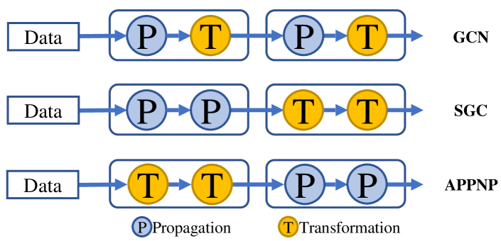
Figure 1: Entanglement of GNNs.

3.2 Pipeline Pattern and Depth

The number of P and T operations plays a very important role in GNN learning.. As introduced in previous studies (Wu et al., 2019; Liu et al., 2020; Miao et al., 2021a), more P operations are required to enhance the information propagation when the edges, labels or features are sparse. In addition, it is widely recognized that more training parameters and T operations should be used to increase the expressive power of neural networks when the size of dataset (i.e., the number of nodes in a graph) is large.

Besides the number of P and T operations, the pipeline pattern (i.e., permutations and combinations) of P and T operations also matters. To verify this, we fix the depths of P and T operations to 2 and only change the pipeline pattern. We evaluate the three architectures in Figure 1, and report their test accuracy on three citation networks. The experimental results in Table 1 show that the test accuracy varies a lot in the pipeline pattern. Concretely, the TTPP architecture achieves the best performance on PubMed, while it is less competitive than the PPTT architecture on Cora and Citeseer. Since the pipeline pattern highly influences the architecture performance and the optimal pipeline pattern varies across different graph datasets, it is necessary to consider the pipeline pattern given a specific dataset/task.

3.3 Influence on smoothness

It is widely recognized that the propagation operation in GNN is a Laplacian smoothing, which may lead to indistinguishable node representations  (Li et al., 2018). In other words, the representations for all nodes will converge to the same value when GNNs go deeper, which is also called over-smoothing. In fact, most entangled GNNs (e.g., GCN and GAT) face the over-smoothing problem and suffer from performance degradation when stacking too many GNN layers. To better measure the influence of P and T operations on smoothness, we analyze the change of smoothness when adding a single P or T operation each time.

Table 1: Test accuracy of GNNs with different PT orders.

Methods	Cora	Citeseer	PubMed
PPTT	83.4$\pm$0.3	72.2$\pm$0.4	78.5$\pm$0.5
TTPP	82.8$\pm$0.2	71.8$\pm$0.3	79.8$\pm$0.3
PTPT	81.2$\pm$0.6	71.2$\pm$0.4	79.1$\pm$0.2

We measure the smoothness by calculating the average similarity (Liu et al., 2020) between two different node embeddings after a P or T operation. Concretely, the node smoothness is defined as follows,

$$\small S^{t}_{i}=1-\frac{1}{2N-2}\sum_{j\in\mathcal{V},j\neq i}\left\|\frac{\mathbf{e}^{t}_{i}}{||\mathbf{e}^{t}_{i}||}-\frac{\mathbf{e}^{t}_{j}}{||\mathbf{e}^{t}_{j}||}\right\|,$$ (3)

where $\mathbf{e}^{t}_{i}$ is the $i$-th node embedding of the $t$-th GNN layer, and $S^{t}_{i}$ measures the similarity of $\mathbf{e}^{t}_{i}$ to the entire graph. Larger $\mathbf{e}^{t}_{i}$ means node $i$ faces higher risk of over-smoothing issue, and $S^{t}_{i}$ ranges in $[0,1]$ since we adopt the normalized node embedding to compute their Euclidean distance. Based on the node smoothness $S^{t}_{i}$, we further measure the average similarities between all the node pairs and define the smoothness of the whole graph $\mathcal{G}$ as:

$$\small S^{t}=\frac{1}{N}\sum_{i\in\mathcal{V}}S^{t}_{i},$$ (4)

where $S^{t}$ is the graph smoothness of the $t$-th GNN layer.

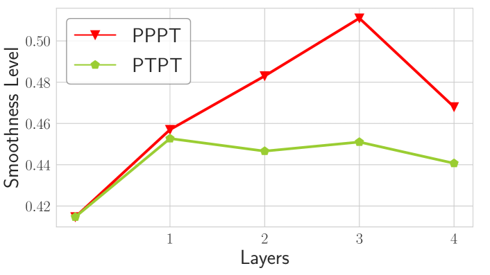
Figure 2: Smoothness of different PT orders.

Unlike previous G-NAS methods that treat the combination of P T as one GNN layer, we treat each P or T here as an individual layer. We change different permutations and combinations of P and T, and report the corresponding output smoothness of each layer in SGC and GCN on Cora. As shown in Figure 2, the results show that 1) the smoothness increases, i.e., the node embedding becomes similar, by applying the P operation; 2) the smoothness decreases by applying the T operation, which implies that the T operation has the ability to alleviate the over-smoothing issue. While over-smoothing leads to indistinguishable node embedding, under-smoothing cannot unleash the full potential of the graph structure. Therefore, how to carefully control the smoothness with P or T in GNNs is also an open question.

4 The Proposed Method

Based on the message passing dis-aggregation, we propose a general design space for GNN pipeline search, which includes the crucial aspects of the number, and the permutations and combinations of P and T operations. Then we provides a custom-designed genetic algorithm to search the space of pipeline pattern and depth.

4.1 Pipeline Search Space

Our general search space of GNNs pipeline includes P-T permutations and combinations, and the number of P-T operations. Besides, we further add connections among each type of operation to enable deep propagation and transformation in DFG-NAS. Suppose a single P or T operation is one GNN layer in DFG-NAS, $\mathbf{o}^{(l)}_{v}$ is the output of node $v$ in the $l$-th layer, $L_{P}$ and $L_{T}$ are two sets that include the layer index of all P operations and T operations, respectively. The layer connections between different layers is as follows.

Propagation Connection. As introduced in Section 3.3, GNNs may suffer from the over-smoothing or under-smoothing issue if we execute too many or too few propagation operations. In addition, a previous study (Zhang et al., 2021b) shows that the nodes with different local structures have different smoothing speeds. Therefore, how to control the smoothness of different nodes in a node-adaptive way is essential in GNN architecture design.

To allow deep propagation and provide suitable smoothness for different nodes, we adopt a gating mechanism upon P operations. The output of the $l$-th P operation is the propagated node embedding of $\mathbf{o}^{(l-1)}$ if its next operation is P. As shown in Figure 3, if the next operation is T, we assign a node-adaptive combination weight for the node embeddings propagated by all previous P operations. The above process can be formulated as,

$$\mathbf{z}^{(l)}_{v} =\textbf{{P}}(\mathbf{o}^{(l-1)}_{v}),$$ (5)

$$\mathbf{o}^{(l)}_{v} =\left\{\begin{aligned} &\mathbf{z}^{(l)}_{v},&\text{Followed by}\ \textbf{{P}}\\ &\sum_{i\in L_{P},i\leq l}\text{Softmax}(\alpha_{i})\mathbf{z}_{v}^{(i)},&\text{Followed by}\ \textbf{{T}}\\ \end{aligned}\right.,$$

where $\alpha_{i}=\sigma(\mathbf{s}\cdot\mathbf{o}_{v}^{i})$ is the weight for $i$-th layer output of node $v$. $\mathbf{s}$ is the trainable vector shared by all nodes , and $\sigma$ denotes the Sigmoid function We adopt the Softmax function to scale the sum of gating scores to 1.

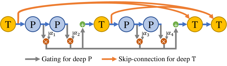
Figure 3: GNN pipeline example in the search space of DFG-NAS.

Transformation Connection. GNNs require more training parameters and non-linear transformation operations to enhance their expressive power on larger graphs. However, it is widely acknowledged that too many transformation operations will lead to the model degradation issue (He et al., 2016), i.e., both the training and test accuracies decrease along with the increased transformation steps.

To allow deeper transformation and meanwhile alleviate the model degradation issue, we introduce the skip-connection mechanism into T operations. As shown in Figure 3, the input of each T operation is the sum of the output of the last layer and the outputs of all previous T operations before the last layer. Concretely, the input and output of the $l$-th T operation can be defined as follows:

$$\small\mathbf{z}^{(l)}_{v} =\mathbf{o}^{(l-1)}_{v}+\sum_{i\in L_{T},i<m(l)}\mathbf{o}^{(i)}_{v},$$ (6)

$$\mathbf{o}^{(l)}_{v} =\sigma\left(\textbf{z}^{(l)}_{v}\mathbf{W}^{(l)}\right),$$

where $m(l)$ is the index of the last T operation before the $l$-th layer, and $\mathbf{W}^{(l)}$ is the learnable parameter in the $l$-th T operation. Specifically, the first layer in our search space is a T operation, and $\mathbf{z}^{(1)}$ refers to the original node features.

4.2 Search via Genetic Algorithm

Genetic algorithm (GA) aims to evolve and improve an entire population of individuals via nature-inspired mechanisms such as mutations. In DFG-NAS, an individual’s chromosome represents a GNN pipeline. To create a new generation of individuals, we perform the following mutations on the chromosomes of the current generation.

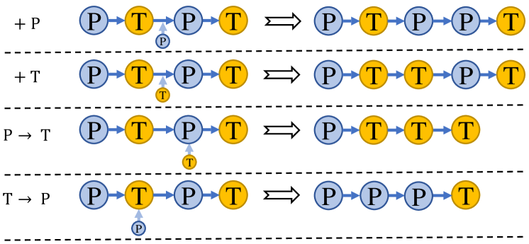
Figure 4: Overview of four different mutations.

Mutation Designs.   Evolutionary algorithms are a class of optimization algorithms inspired by biological evolution. Specifically, they apply mutations on a population of designs, i.e., the set of different GNN architectures. In DFG-NAS, each GNN architecture is encoded as a sequence consisting of the P and T operations. As shown in Figure 4, we design four mutations, which are as follows,

Case 1 + P: Add a propagation operation.

Case 2 + T: Add a transformation operation.

Case 3 P $\rightarrow$ T: Replace a propagation operation by a transformation operation.

Case 4 T $\rightarrow$ P: Replace a transformation operation by a propagation operation.

The above four mutations take place at a random position of the sequence. For example, we can add a propagation operation after or before any other operations. These four specific mutations are proposed for their similarity to the actions that a human designer may take when improving the GNN architecture.

Evolutionary Algorithm.  To perform an efficient and effective search on our search space, we adopt the evolutionary algorithm as the searching method, which is a class of optimization algorithms inspired by biological evolution. The concrete searching pipeline is summarized in Algorithm 1.

We randomly generate $k$ different GNN architectures as initial individuals in a population set $\mathbf{Q}$ (line 1), and then evaluate these GNNs on the validation set (line 2). Next, we randomly sample $m$ ($m<k$) individuals from the population (line 4) and select the architecture with the best validation performance as parent $A$ (line 5). After that, the child GNN architecture $B$ is generated by randomly picking one of the four mutations (i.e., + P, + T, P $\rightarrow$ T, or T $\rightarrow$ P) introduced in Section 4.2. At last, $B$ is evaluated and added to the population (line 7), and then the oldest individual in $\mathbf{Q}$ is removed (line 8). The above process is repeated for $T$ generations and finally returns the architecture with the best observed evaluation performance (line 9).

Input: The population set $\mathbf{Q}$, the maximum generation times $T$, the generation number $t=1$.

Output: The best GNN architecture.

Algorithm 1 Searching method.

Initialize the population set $\mathbf{Q}$ with $|\mathbf{Q}|=k$;

Evaluating $k$ different GNN architectures in $\mathbf{Q}$;

for $1\leq t\leq T$ do

2       Randomly sample $m$ individuals from $\mathbf{Q}$; Select the parent $A$ with best evaluation performance from the $m$ individuals; Randomly mutate $A$ with the mutation designs, and get the mutated individual $B$; Evaluate $B$ and adding it to $\mathbf{Q}$; Remove the oldest individual in $\mathbf{Q}$;

return the individual with best evaluation performance.

4.3 Relationship with Existing Literature

The proposed DFG-NAS differs from existing G-NAS methods in both the pipeline pattern and pipeline depth of the searched architectures.

Fixed vs. Flexible. The existing G-NAS methods treat the combination of propagation and transformation as one GNN layer, which leads to a fixed pipeline pattern. Instead, DFG-NAS disentangles the propagation and transformation operations and thus enjoys better flexibility.

Shallow vs. Deep. The over-smoothing issue in deep GNNs has not been well studied and considered in the search space of the existing methods. For example, both GraphNAS and AutoGNN adopt a search space that applies a fixed three-layer GNN as the macro-architecture. DFG-NAS enables both deep P and T with the gating mechanism and skip-connection mechanism, respectively.

Note that DFG-NAS mainly focuses on GNN macro-architecture search, so it is orthogonal to and compatible with the GNN micro-architecture search space (e.g, aggregation/activation functions, batch normalization, etc.) used by existing G-NAS methods.

5 Experiments and Results

To evaluate DFG-NAS, we apply it on four public graph datasets. Compared with the state-of-the-art baselines, we list three main insights that we will investigate as follows,

• DFG-NAS generates more powerful architectures than state-of-the-art manual designs.

• DFG-NAS works more efficiently than other NAS methods for GNN. It reaches similar performance to other methods while spending less search time.

• DFG-NAS is able to tackle the two limitations as mentioned in Section 1. Concretely, the Gate operation helps avoid over-smoothing while the disentanglement of P and T increases architecture flexibility.

5.1 Experimental Setup

Baselines.   We compare our proposed method DFG-NAS with nine manual GNN architectures and three NAS methods for GNN. The manual designs include the following three types of GNNs according to their pipeline pattern of propagation (P) and transformation (T) operations.

• Alternate P and T: GCN  (Kipf & Welling, 2017), GraphSAGE  (Hamilton et al., 2017), and GAT  (Veličković et al., 2017). The propagation operation P and transformation operation T are intertwined and executed alternately in these entangled GNNs.

• T before P: APPNP (Klicpera et al., 2019), AP-GCN (Spinelli et al., 2021), and DAGNN (Liu et al., 2020). These disentangled GNNs firstly transform the node features with T operations, and then propagate the outputs with multiple P operations.

• P before T: SGC (Wu et al., 2019) , SIGN (Rossi et al., 2020), and S²GC (Zhu & Koniusz, 2021). On contrary to APPNP, these disentangled GNNs execute multiple P operations in advance, and then transform propagated features with T operations.

More details of the above manual methods are provided in Appendix A.3. Besides, the compared G-NAS methods include: (1) Auto-GNN (Zhou et al., 2019): a reinforced conservative search strategy by adopting both RNNs and evolutionary algorithms in the controller; (2) GraphNAS (Gao et al., 2020a): a reinforcement learning-based method that uses an RNN controller to sample from the multiple architectures sequentially; (3) GraphGym (You et al., 2020): a variant of random search on a general GNN search space that considers intra-layer design, inter-layer design, and training configurations.

Datasets.   We conduct the experiments on four public graph datasets: three citation graphs (Cora, Citeseer and PubMed) (Kipf & Welling, 2017), and one large OGB graph (ogbn-arxiv) (Hu et al., 2020). We follow the public training/validation/test split for three citation networks and adopt the official split in the OGB graph. The statistics of these datasets are summarized in Appendix A.1.

Experimental Settings.   For a fair end-to-end comparison on each task, we run DFG-NAS for 500 iterations, and set the time cost as the budget for other G-NAS baselines. Then we report the average best observed test accuracy of the searched architecture. Specifically, we re-training each searched architecture ten times to avoid randomness. These baselines are implemented based on their open-sourced version. Since AutoGNN is not publicly available, we only report its performance on citation graphs following its paper. The details of hyperparameters and reproduction instructions are provided in Appendix A.2 and A.5.

Table 2: Test accuracy on the node classification task.

Methods	Cora	Citeseer	PubMed	ogbn-arxiv
Alternate P and T
GCN	81.3$\pm$0.6	71.1$\pm$0.1	78.8$\pm$0.4	71.7$\pm$0.3
GAT	82.9$\pm$0.2	70.8$\pm$0.5	79.1$\pm$0.1	71.9$\pm$0.2
GraphSAGE	79.2$\pm$0.6	71.6$\pm$0.5	77.4$\pm$0.5	71.5$\pm$0.3
T before P
APPNP	83.1$\pm$0.5	71.8$\pm$0.4	80.1$\pm$0.2	72.0$\pm$0.1
AP-GCN	83.4$\pm$0.3	71.3$\pm$0.5	79.7$\pm$0.3	71.9$\pm$0.2
DAGNN	84.3$\pm$0.2	73.3$\pm$0.6	80.5$\pm$0.5	72.0$\pm$0.3
P before T
SGC	81.7$\pm$0.2	71.3$\pm$0.2	78.8$\pm$0.1	71.6$\pm$0.3
SIGN	82.1$\pm$0.3	72.4$\pm$0.8	79.5$\pm$0.5	71.9$\pm$0.1
S2GC	82.7$\pm$0.3	73.0$\pm$0.2	79.9$\pm$0.3	71.8$\pm$0.3
G-NAS Methods
GraphNAS	83.7$\pm$0.4	73.5$\pm$0.3	80.5$\pm$0.3	71.7$\pm$0.2
AutoGNN	83.6$\pm$0.3	73.8$\pm$0.7	79.7$\pm$0.4	/
GraphGym	83.5$\pm$0.2	73.4$\pm$0.3	80.3$\pm$0.2	71.6$\pm$0.3
DFG-NAS	85.2$\pm$0.2	74.1$\pm$0.4	81.1$\pm$0.3	72.3$\pm$0.2

5.2 Comparison with Existing GNNs

We first compare the architectures obtained by DFG-NAS with state-of-the-art manual designs on four datasets in Table 2. The structures of the searched architectures are provided in Appendix A.6. Among the manual designs, DAGNN achieves stable and competitive performance on four datasets. The reason is that it applies a single Gate operation to combine all propagation outputs, and in this way, it allows a deeper propagation than other manual designs. However, DAGNN employs the straight-forward MLP for transformation, which may lead to the model degradation issue when transformation goes deeper. In addition, as all the compared manual designs follow a specific pipeline pattern of P and T, their performance can not be further improved due to their restricted flexibility. As a result, DFG-NAS obtains the deepest architectures with high expressive power and achieves the best performance on all four datasets. Remarkably, the architecture searched by DFG-NAS on the large-scale ogbn-arxiv dataset contains 27 P and 16 T operations, and it outperforms the best manual design DAGNN by a margin of 0.3% on test accuracy.

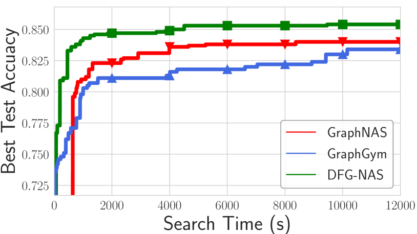
(a) Cora

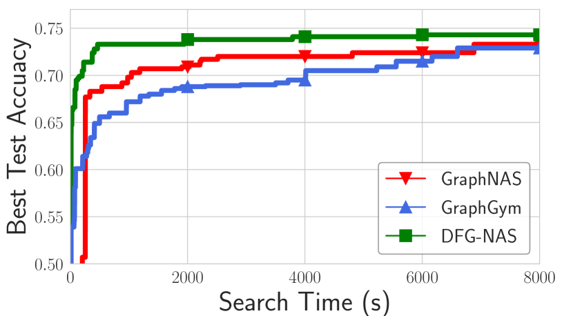
(b) Citeseer

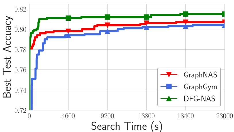
(c) Pubmed

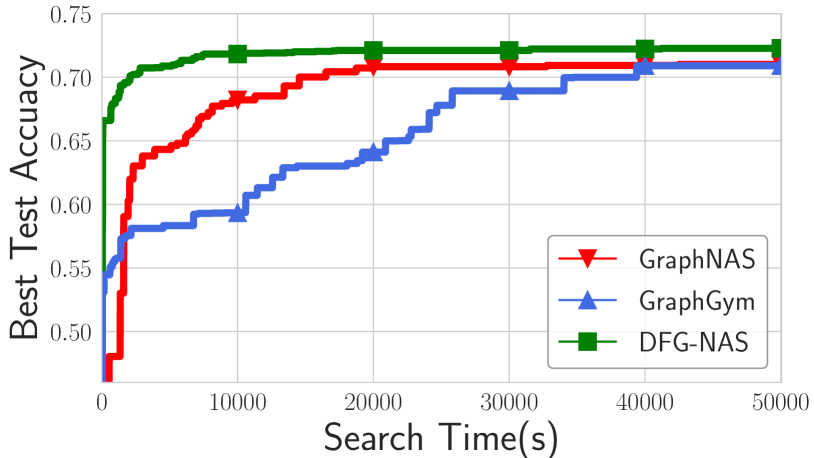
(d) ogbn-arxiv

Figure 5: Test results during neural architecture search on four datasets.

Table 3: Ablation study on Gate operations.

Methods	Cora	Citeseer	PubMed	ogbn-arxiv
A w/o Gate	82.0$\pm$0.3	70.8$\pm$0.5	78.1$\pm$0.1	68.5$\pm$0.6
S w/o Gate	83.6$\pm$0.2	72.6$\pm$0.2	79.3$\pm$0.3	71.5$\pm$0.4
DFG-NAS	85.2$\pm$0.2	74.1$\pm$0.4	81.1$\pm$0.3	72.3$\pm$0.2

5.3 Comparison with NAS methods

Figure 5 and Table 2 demonstrate the performance of DFG-NAS compared with existing NAS methods for GNN. Since AutoGNN is not open-sourced, we only report the results on three datasets from its paper. From Figure 5, we observe that DFG-NAS consistently outperforms the compared NAS methods. The main reason is that the existing NAS methods only consider a fixed pipeline pattern of propagation and transformation operations in their architecture design, which may not be the optimal order as introduced in Section 3.2. When the search budget exhausts, DFG-NAS outperforms the second-best baseline by a margin of 0.3-1.5% on test accuracy. Compared with the second-best baseline GraphNAS, DFG-NAS achieves 6.97-15.96x speedups when achieving the same test accuracy on four datasets, which indicates the superior efficiency of our proposed method.

5.4 Ablation Study

In this part, we present an ablation study to show the effectiveness of three designs in DFG-NAS, which are 1) the Gate operation; 2) the disentanglement of architectures and 3) the skip-connection operation.

In Table 3, we compare DFG-NAS with two baselines: 1) A w/o Gate: the resulting architecture with the Gate operation disabled and 2) S w/o Gate: the searched results over a reduced space without the Gate operation in architecture design. We observe that the accuracy declines on all datasets. Remarkably, the accuracy drops by 3.0-3.8% for architectures without Gate. The reason is that without the Gate operation, the transformation steps only take the last output of the propagation steps as inputs, which may suffer from a risk of over-smoothing. The Gate operation dynamically aggregates the information from all propagation steps and thus controls the smoothness of different nodes in a node-adaptive way. In addition, when the Gate operation is removed from the architecture space, the accuracy drops by 0.8-1.8%. In this setting, the searched architectures tend to have shallow propagation (i.e., only 3-5 steps) on all datasets, which is not enough to capture sufficient neighborhood information for each node. These ablation results demonstrate the importance of the gating mechanism on GNN architecture design.

Table 4: Ablation study on pipeline pattern.

Methods	Cora	Citeseer	PubMed	ogbn-arxiv
P before T	83.2$\pm$0.3	72.7$\pm$0.2	80.0$\pm$0.4	69.4$\pm$0.1
T before P	83.6$\pm$0.5	71.8$\pm$0.3	79.0$\pm$0.5	70.0$\pm$0.1
Alternate P and T	82.5$\pm$0.4	69.9$\pm$0.6	78.1$\pm$0.3	68.1$\pm$0.4
DFG-NAS	85.2$\pm$0.2	74.1$\pm$0.4	81.1$\pm$0.3	72.3$\pm$0.2

Table 5: Ablation study on skip-connection.

Methods	Cora	Citeseer	PubMed
A w/o Skip	83.7$\pm$0.5	71.6$\pm$0.5	81.0$\pm$0.3
S w/o Skip	83.9$\pm$0.4	72.8$\pm$0.6	80.6$\pm$0.2
DFG-NAS	85.2$\pm$0.2	74.1$\pm$0.4	81.1$\pm$0.3

To show the flexibility of the search space in DFG-NAS, we consider the following search spaces inspired by existing designs of propagation (P) and transformation (T): (1) P before T, (2) T before P, and (3) alternate P and T. The depths of P and T range from 1 to 10, which leads to 100 unique architectures in (1) and (2), and ten unique architectures in (3). We exhaustively evaluate all possible architectures in the baseline search space, and Table 4 shows the best observed performance over each search space. Among the baselines, alternate P and T has the worst performance, which is consistent with the observations in previous studies (Liu et al., 2020). In addition, none of the three baselines dominate the others on all datasets, which indicates the necessity of a more flexible search on macro-architecture. Since the search space of DFG-NAS does not restrict the pipeline pattern of P and T, the space of DFG-NAS covers the compared baselines, and the architectures are more flexible than those from the baselines. As a result, DFG-NAS achieves an increase of 1.1% to 2.3% on all datasets.

To show the effectiveness of skip-connection. In Table 5, we compare DFG-NAS with two baselines: 1) A w/o Skip: the resulting architecture with the Skip-connection disabled and 2) S w/o Skip: the searched results over a reduced space without the skip-connection in architecture design. We observe that the accuracy declines on all datasets. And we also find when the skip-connection is removed from the search space, the architectures searched by our method will have less T operations.

To summarize, the searched architecture performance is improved by introducing the Gate operation in propagation steps, disentangling P and T in architecture designs, and the skip-connection in T operations. All of them may help unleash the full potential of GNNs and inspire more powerful manual designs.

5.5 Interpretability

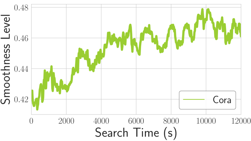
(a) Cora

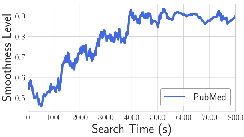
(b) Pubmed

Figure 6: Average smoothness over iterations on two datasets.

In Figure 6, we plot the average smoothness of the last layer outputs of architectures in the population during each iteration on two datasets. The definition of smoothness is provided in Equation 4. Though graph datasets differ in the requirement of smoothness, both two curves are generally saturating. In the first half of the search process, the smoothness quickly increases due to the frequent elimination of bad initial individuals. Then, the smoothness fluctuates around a certain level (0.46 for Cora and 0.90 for Pubmed), which implies that the search algorithm in DFG-NAS can ensure sufficient smoothness of inputs in the searched architectures, and meanwhile avoid over-smoothing.

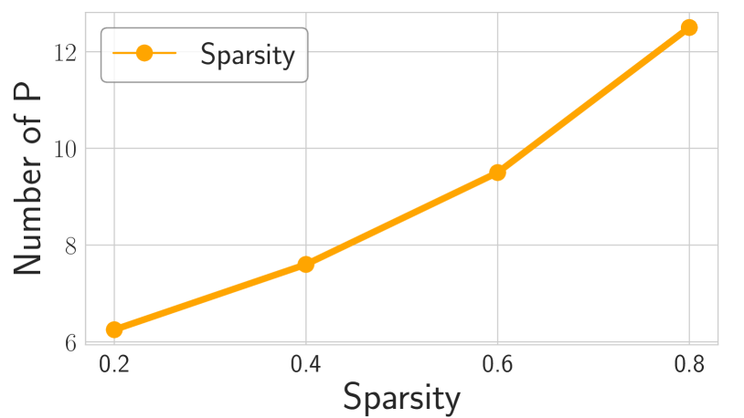
(a) Trend of P on sparsity

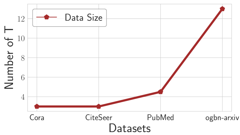
(b) Trend of T on data size

Figure 7: Left: Average number of P operations along with the increased sparsity on PubMed. Right: Average number of T operations along with the increased nodes of different datasets.

Finally, we study how the sparsity and size of datasets influence the number of P and T in the searched architectures, respectively. To simulate datasets with different sparsity, we randomly delete some of the edges in PubMed. Figure 7(a) shows that the average number of P in top-10 architectures increases when the dataset grows sparser. The reason is that, when the graph is sparse, the architecture should contain more propagation steps so that each node is able to capture sufficient neighborhood information for classification. On the other hand, when the size of datasets grows larger, the architecture should include more transformation steps to ensure the expressive power. As shown in Figure 7(b), the average number of T is similar in Core and Citeseer, which includes about 3k samples. The number further increases to 4.5 and 13.0 on larger datasets PubMed and ogbn-arxiv with 20k and 169k samples, respectively. The trend of P and T discovered by DFG-NAS may help guide the manual design of flexible GNN architectures, i.e., more propagation steps are required when the graph is sparse, while more transformation steps are needed for the large graph.

6 Conclusion

In this paper, we proposed DFG-NAS, a new method that allows both flexible and deep graph neural architecture search. The key idea of DFG-NAS is to dis-aggregate the design pipeline of GNN generation, allowing a flexible permutations and combinations of the two basic operations in GNNs: propagation and transformation. In addition, we also analyzed how both operations influence the smoothness. Based on the observation, we adopted the gating mechanism and skip-connection mechanisms to support very deep GNN pipelines. We provided the genetic algorithm to search for a good permutations and combinations in GNNs. The experimental results on four different graph datasets showed that DFG-NAS achieves an accuracy improvement of up to 0.9% over state-of-the-art manual designs and brings up to 15.96x speedups over existing G-NAS methods.

Appendix A Outline

The appendix is organized as follows:

A.1

Datasets Description.

A.2

Hyper-parameters Setting.

A.3

Compared Baselines.

A.4

Efficiency Analysis.

A.5

Reproduction Instructions.

A.6

The Best Architecture Searched by DFG-NAS.

A.1 Dataset Description

Cora, Citeseer, and Pubmed are three popular citation network datasets, and we follow the public training/validation/test split in GCN  (Kipf & Welling, 2017). In these three networks, papers from different topics are considered as nodes, and the edges are citations among the papers. The node attributes are binary word vectors, and class labels are the topics papers belong to.

ogbn-arxiv is a directed graph, representing the citation network among all Computer Science (CS) arXiv papers indexed by MAG. The training/validation/test split in our experiment is the same as the public version. The public version provided by OGBis used in our paper.

A.2 Hyper-parameters Setting

For the architecture search, the number of the population set $k$ and the maximum generation times $T$ in Algorithm 1 are 20 and 500 for all datasets. For the training of GNN architectures, we follow the same hyper-parameter in their original paper and tune it with OpenBox (Li et al., 2021a). The training budget of each searched GNN architecture in DFG-NAS is 200 epochs for three citation networks and 500 epochs for the ogbn-arxiv dataset. Specifically, we train them using Adam optimizer with a learning rate of 0.02 for Cora, 0.03 for Citeseer, 0.1 for PubMed, and 0.001 for ogbn-arxiv. The regularization factor is 5e-4 for all datasets. We apply dropout to all feature vectors with rates of 0.5 for Cora and Citeseer, and 0.3 for PubMed and ogbn-arxiv. Besides, the dropout between different GNN layers is 0.8 for Cora and Citeseer, and 0.5 for PubMed and ogbn-arxiv. At last, the hidden size of each GNN layer is 128 for Cora and ogbn-arxiv, 256 for Citeseer, and 512 for ogbn-arxiv.

Table 6: Overview of the Four Datasets.

Dataset	#Nodes	#Features	#Edges	#Classes	#Train/Val/Test
Cora	2,708	1,433	5,429	7	1,208/500/1,000
Citeseer	3,327	3,703	4,732	6	1,827/500/1,000
Pubmed	19,717	500	44,338	3	18,217/500/1,000
ogbn-arxiv	169,343	128	1,166,243	40	90,941/29,799/48,603

Table 7: The searched GNN architecture in different datasets.

Datasets	Searched Architectures (in sequence)
Cora	[T, P, P, P, P, P, T, P, P, T]
Citeseer	[T, P, P, P, P, P, P, P, P, P, P, P, T, P, T]
PubMed	[T, P, P, P, P, P, P, P, P, P, P, P, P, P, P, P, P, P, P, P, P, P, P, T]
ogbn-arxiv	[T, P, P, P, P, P, P, P, P, P, P, T, T, P, P, P, T, P, T, P, P, T, T, P, P, T, T, T, P, T, P, P, P, T, T, P, T, P, T, P, P, T, P, T, T]

A.3 Compared Baselines.

For existing manual GNNs, we summarize the existing baselines according to the pipeline pattern of propagation (P) and transformation (T) operations. Specifically, they can be classified into the following three types.

(1) Alternate P and T:

• Graph Convolutional Network(GCN)  (Kipf & Welling, 2017): GCN adopts an efficient layer-wise propagation rule that is based on a first-order approx- imation of spectral convolutions on graphs.

• Graph Attention Networks(GAT)  (Veličković et al., 2017): GAT leverages masked self-attention layers to specify different weights to different nodes in a neighborhood, thus better represent graph information.

• GraphSAGE  (Hamilton et al., 2017): GraphSAGE is an inductive framework that leverages node attribute information to efficiently generate representations on previously unseen data.

(2) P before T:

• Simplified GCN (SGC)  (Wu et al., 2019): SGC simplifies GCN by removing nonlinearities and collapsing weight matrices between consecutive layers.

• Scalable Inception Graph Neural Networks (SIGN)  (Rossi et al., 2020): SIGN is an efficient and scalable graph embedding method that sidesteps graph sampling in GCN and uses different local graph operators to support different tasks.

• Simple Spectral Graph Convolution (S²GC) (Zhu & Koniusz, 2021): S²GC is a trade-off of low- and high-pass filter bands which capture the global and local contexts of each node

(3) T before P

• APPNP  (Klicpera et al., 2019): APPNP has the ability to use the relationship between graph convolution networks (GCN) and PageRank to derive improved node representations.

• Adaptive Propagation Graph Convolution Network (AP-GCN)  (Spinelli et al., 2021): AP-GCN uses a halting unit to decide a receptive range of a given node.

• Deep Adaptive Graph Neural Network (DAGNN): DAGNN decouples the propagation and transformation operations, and it can adaptively incorporate information from large receptive fields.

For G-NAS methods, the compared baselines are as follows:

• Auto-GNN (Zhou et al., 2019): Auto-GNN is a reinforced conservative search strategy by adopting both RNNs and evolutionary algorithms in the controller.

• GraphNAS (Gao et al., 2020a): GraphNAS is a reinforcement learning-based method that uses an RNN controller to sample from the multiple architectures sequentially.

• GraphGym (You et al., 2020): GraphGym is a variant of random search on a general GNN search space that considers intra-layer design, inter-layer design, and training configurations.

Note that we implement GraphNAS  and GraphGym  according to their open-sourced version.

A.4 Efficiency Analysis

The time complexity of the EA method is $O(m)$, where $m$ is the population size. In other words, the method is independent of the number of evaluations, and runs as fast as random search. While P or T can be added infinitely, previous methods for finite spaces can not be directly applied to our design space. And thus we perform the end-to-end comparisons in our paper. Figure 5 shows that DFG-NAS achieves similar performance to other methods with less search time. As our searching algorithm is relatively simple, we attribute this gain to the design of our search space, i.e., the well-designed architecture in our search space outperforms the precious ones.

A.5 Reproduction Instructions

The experiments are conducted on a machine with Intel(R) Xeon(R) Gold 5120 CPU @ 2.20GHz, and a single NVIDIA TITAN RTX GPU with 24GB GPU memory. The operating system of the machine is Ubuntu 16.04. For software versions, we use Python 3.6, Pytorch 1.7.1, and CUDA 10.1. Our code is available in the anonymized repository https://github.com/PKU-DAIR/DFG-NAS.

A.6 The Best Architecture Searched by DFG-NAS

The best GNN architecture searched by DFG-NAS on different graph datasets is summarized in Table 7. Note that each GNN architecture will begin with a T operation for dimension reduction and end with a T operation for getting the softmax outputs.

References

- Bradshaw et al. (2019) Bradshaw, J., Kusner, M. J., Paige, B., Segler, M. H. S., and Hernández-Lobato, J. M. A generative model for electron paths. In 7th International Conference on Learning Representations, ICLR 2019, New Orleans, LA, USA, May 6-9, 2019, 2019.
- Cai et al. (2021) Cai, S., Li, L., Deng, J., Zhang, B., Zha, Z.-J., Su, L., and Huang, Q. Rethinking graph neural architecture search from message-passing. In Proceedings of the IEEE/CVF Conference on Computer Vision and Pattern Recognition, pp. 6657–6666, 2021.
- Dai et al. (2019) Dai, H., Li, C., Coley, C. W., Dai, B., and Song, L. Retrosynthesis prediction with conditional graph logic network. In Advances in Neural Information Processing Systems 32: Annual Conference on Neural Information Processing Systems 2019, NeurIPS 2019, December 8-14, 2019, Vancouver, BC, Canada, pp. 8870–8880, 2019.
- Frasca et al. (2020) Frasca, F., Rossi, E., Eynard, D., Chamberlain, B., Bronstein, M., and Monti, F. Sign: Scalable inception graph neural networks. In ICML 2020 Workshop on Graph Representation Learning and Beyond, 2020.
- Gao et al. (2020a) Gao, Y., Yang, H., Zhang, P., Zhou, C., and Hu, Y. Graph neural architecture search. In Bessiere, C. (ed.), Proceedings of the Twenty-Ninth International Joint Conference on Artificial Intelligence, IJCAI 2020, pp. 1403–1409. ijcai.org, 2020a.
- Gao et al. (2020b) Gao, Y., Yang, H., Zhang, P., Zhou, C., and Hu, Y. Graph neural architecture search. In IJCAI, volume 20, pp. 1403–1409, 2020b.
- Hamilton et al. (2017) Hamilton, W., Ying, Z., and Leskovec, J. Inductive representation learning on large graphs. In NIPS, pp. 1024–1034, 2017.
- He et al. (2016) He, K., Zhang, X., Ren, S., and Sun, J. Deep residual learning for image recognition. In Proceedings of the IEEE conference on computer vision and pattern recognition, pp. 770–778, 2016.
- He et al. (2020) He, X., Deng, K., Wang, X., Li, Y., Zhang, Y., and Wang, M. Lightgcn: Simplifying and powering graph convolution network for recommendation. In Proceedings of the 43rd International ACM SIGIR conference on research and development in Information Retrieval, SIGIR 2020, Virtual Event, China, July 25-30, 2020, pp. 639–648, 2020.
- Hu et al. (2020) Hu, W., Fey, M., Zitnik, M., Dong, Y., Ren, H., Liu, B., Catasta, M., and Leskovec, J. Open graph benchmark: Datasets for machine learning on graphs. In Larochelle, H., Ranzato, M., Hadsell, R., Balcan, M., and Lin, H. (eds.), Advances in Neural Information Processing Systems 33: Annual Conference on Neural Information Processing Systems 2020, NeurIPS 2020, December 6-12, 2020, virtual, 2020.
- Huan et al. (2021) Huan, Z., Quanming, Y., and Weiwei, T. Search to aggregate neighborhood for graph neural network. In 2021 IEEE 37th International Conference on Data Engineering (ICDE), pp. 552–563. IEEE, 2021.
- Huang et al. (2021) Huang, C., Xu, H., Xu, Y., Dai, P., Xia, L., Lu, M., Bo, L., Xing, H., Lai, X., and Ye, Y. Knowledge-aware coupled graph neural network for social recommendation. In AAAI Conference on Artificial Intelligence (AAAI), 2021.
- Huang et al. (2017) Huang, G., Liu, Z., Van Der Maaten, L., and Weinberger, K. Q. Densely connected convolutional networks. In Proceedings of the IEEE conference on computer vision and pattern recognition, pp. 4700–4708, 2017.
- Jiang et al. (2022) Jiang, Y., Cheng, Y., Zhao, H., Zhang, W., Miao, X., He, Y., Wang, L., Yang, Z., and Cui, B. Zoomer: Boosting retrieval on web-scale graphs by regions of interest. arXiv preprint arXiv:2203.12596, 2022.
- Kipf & Welling (2017) Kipf, T. N. and Welling, M. Semi-supervised classification with graph convolutional networks. In ICLR, 2017.
- Klicpera et al. (2019) Klicpera, J., Bojchevski, A., and Günnemann, S. Predict then propagate: Graph neural networks meet personalized pagerank. In 7th International Conference on Learning Representations, ICLR 2019, New Orleans, LA, USA, May 6-9, 2019. OpenReview.net, 2019.
- Li et al. (2019) Li, G., Muller, M., Thabet, A., and Ghanem, B. Deepgcns: Can gcns go as deep as cnns? In Proceedings of the IEEE/CVF International Conference on Computer Vision, pp. 9267–9276, 2019.
- Li et al. (2018) Li, Q., Han, Z., and Wu, X.-M. Deeper insights into graph convolutional networks for semi-supervised learning. In Proceedings of the AAAI Conference on Artificial Intelligence, volume 32, 2018.
- Li et al. (2021a) Li, Y., Shen, Y., Zhang, W., Chen, Y., Jiang, H., Liu, M., Jiang, J., Gao, J., Wu, W., Yang, Z., et al. Openbox: A generalized black-box optimization service. arXiv preprint arXiv:2106.00421, 2021a.
- Li et al. (2021b) Li, Y., Wen, Z., Wang, Y., and Xu, C. One-shot graph neural architecture search with dynamic search space. In Proceedings of the AAAI Conference on Artificial Intelligence, volume 35, pp. 8510–8517, 2021b.
- Liu et al. (2020) Liu, M., Gao, H., and Ji, S. Towards deeper graph neural networks. In Proceedings of the 26th ACM SIGKDD International Conference on Knowledge Discovery & Data Mining, pp. 338–348, 2020.
- Miao et al. (2021a) Miao, X., Gürel, N. M., Zhang, W., Han, Z., Li, B., Min, W., Rao, S. X., Ren, H., Shan, Y., Shao, Y., et al. Degnn: Improving graph neural networks with graph decomposition. In Proceedings of the 27th ACM SIGKDD Conference on Knowledge Discovery & Data Mining, pp. 1223–1233, 2021a.
- Miao et al. (2021b) Miao, X., Zhang, W., Shao, Y., Cui, B., Chen, L., Zhang, C., and Jiang, J. Lasagne: A multi-layer graph convolutional network framework via node-aware deep architecture. IEEE Transactions on Knowledge and Data Engineering, 2021b.
- Rossi et al. (2020) Rossi, E., Frasca, F., Chamberlain, B., Eynard, D., Bronstein, M., and Monti, F. Sign: Scalable inception graph neural networks. arXiv preprint arXiv:2004.11198, 2020.
- Sarlin et al. (2020) Sarlin, P.-E., DeTone, D., Malisiewicz, T., and Rabinovich, A. Superglue: Learning feature matching with graph neural networks. In Proceedings of the IEEE/CVF conference on computer vision and pattern recognition, pp. 4938–4947, 2020.
- Shi et al. (2019) Shi, L., Zhang, Y., Cheng, J., and Lu, H. Skeleton-based action recognition with directed graph neural networks. In Proceedings of the IEEE/CVF Conference on Computer Vision and Pattern Recognition, pp. 7912–7921, 2019.
- Spinelli et al. (2021) Spinelli, I., Scardapane, S., and Uncini, A. Adaptive propagation graph convolutional network. IEEE Trans. Neural Networks Learn. Syst., 32(10):4755–4760, 2021.
- Vashishth et al. (2020) Vashishth, S., Yadati, N., and Talukdar, P. P. Graph-based deep learning in natural language processing. In Roy, R. S. (ed.), CoDS-COMAD 2020: 7th ACM IKDD CoDS and 25th COMAD, Hyderabad India, January 5-7, 2020, pp. 371–372. ACM, 2020.
- Veličković et al. (2017) Veličković, P., Cucurull, G., Casanova, A., Romero, A., Lio, P., and Bengio, Y. Graph attention networks. arXiv preprint arXiv:1710.10903, 2017.
- Velickovic et al. (2018) Velickovic, P., Cucurull, G., Casanova, A., Romero, A., Liò, P., and Bengio, Y. Graph attention networks. In 6th International Conference on Learning Representations, ICLR 2018, Vancouver, BC, Canada, April 30 - May 3, 2018, Conference Track Proceedings. OpenReview.net, 2018.
- Wang et al. (2021) Wang, G., Ying, R., Huang, J., and Leskovec, J. Multi-hop attention graph neural networks. In Zhou, Z. (ed.), Proceedings of the Thirtieth International Joint Conference on Artificial Intelligence, IJCAI 2021, Virtual Event / Montreal, Canada, 19-27 August 2021, pp. 3089–3096. ijcai.org, 2021.
- Wu et al. (2019) Wu, F., Souza, A., Zhang, T., Fifty, C., Yu, T., and Weinberger, K. Simplifying graph convolutional networks. In International conference on machine learning, pp. 6861–6871. PMLR, 2019.
- Wu et al. (2021) Wu, L., Chen, Y., Shen, K., Guo, X., Gao, H., Li, S., Pei, J., and Long, B. Graph neural networks for natural language processing: A survey. arXiv preprint arXiv:2106.06090, 2021.
- Wu et al. (2020) Wu, S., Sun, F., Zhang, W., Xie, X., and Cui, B. Graph neural networks in recommender systems: a survey. ACM Computing Surveys (CSUR), 2020.
- Xu et al. (2018) Xu, K., Li, C., Tian, Y., Sonobe, T., Kawarabayashi, K., and Jegelka, S. Representation learning on graphs with jumping knowledge networks. In ICML, pp. 5449–5458, 2018.
- You et al. (2020) You, J., Ying, Z., and Leskovec, J. Design space for graph neural networks. Advances in Neural Information Processing Systems, 33, 2020.
- Zeng et al. (2020) Zeng, H., Zhou, H., Srivastava, A., Kannan, R., and Prasanna, V. K. Graphsaint: Graph sampling based inductive learning method. In 8th International Conference on Learning Representations, ICLR 2020, Addis Ababa, Ethiopia, April 26-30, 2020. OpenReview.net, 2020.
- Zhang et al. (2020) Zhang, W., Miao, X., Shao, Y., Jiang, J., Chen, L., Ruas, O., and Cui, B. Reliable data distillation on graph convolutional network. In Proceedings of the 2020 ACM SIGMOD International Conference on Management of Data, pp. 1399–1414, 2020.
- Zhang et al. (2021a) Zhang, W., Sheng, Z., Jiang, Y., Xia, Y., Gao, J., Yang, Z., and Cui, B. Evaluating deep graph neural networks. arXiv preprint arXiv:2108.00955, 2021a.
- Zhang et al. (2021b) Zhang, W., Yang, M., Sheng, Z., Li, Y., Ouyang, W., Tao, Y., Yang, Z., and Cui, B. Node dependent local smoothing for scalable graph learning. Advances in Neural Information Processing Systems, 34, 2021b.
- Zhang et al. (2021c) Zhang, W., Yin, Z., Sheng, Z., Ouyang, W., Li, X., Tao, Y., Yang, Z., and Cui, B. Graph attention multi-layer perceptron. arXiv preprint arXiv:2108.10097, 2021c.
- Zhou et al. (2019) Zhou, K., Song, Q., Huang, X., and Hu, X. Auto-gnn: Neural architecture search of graph neural networks. arXiv preprint arXiv:1909.03184, 2019.
- Zhu & Koniusz (2021) Zhu, H. and Koniusz, P. Simple spectral graph convolution. In International Conference on Learning Representations, 2021.