Query-Efficient and Scalable Black-Box Adversarial Attacks on
Discrete Sequential Data via Bayesian Optimization

Abstract

We focus on the problem of adversarial attacks against models on discrete sequential data in the black-box setting where the attacker aims to craft adversarial examples with limited query access to the victim model. Existing black-box attacks, mostly based on greedy algorithms, find adversarial examples using pre-computed key positions to perturb, which severely limits the search space and might result in suboptimal solutions. To this end, we propose a query-efficient black-box attack using Bayesian optimization, which dynamically computes important positions using an automatic relevance determination (ARD) categorical kernel. We introduce block decomposition and history subsampling techniques to improve the scalability of Bayesian optimization when an input sequence becomes long. Moreover, we develop a post-optimization algorithm that finds adversarial examples with smaller perturbation size. Experiments on natural language and protein classification tasks demonstrate that our method consistently achieves higher attack success rate with significant reduction in query count and modification rate compared to the previous state-of-the-art methods.

1 Introduction

In recent years, deep neural networks on discrete sequential data have achieved remarkable success in various domains including natural language processing and protein structure prediction, with the advent of large-scale sequence models such as BERT and XLNet (BERT; XLNet). However, these networks have exhibited vulnerability against adversarial examples that are artificially crafted to raise network malfunction by adding perturbations imperceptible to humans (papernot2016crafting; TextFooler). Recent works have focused on developing adversarial attacks in the black-box setting, where the adversary can only observe the predicted class probabilities on inputs with a limited number of queries to the network (GA; PWWS). This is a more realistic scenario since, for many commercial systems (google; amazon), the adversary can only query input sequences and receive their prediction scores with restricted resources such as time and cost.

While a large body of works has proposed successful black-box attacks in the image domain with continuous attack spaces (ilyas2018black; andriushchenko2020square), developing a query-efficient black-box attack on discrete sequential data is quite challenging due to the discrete nature of their attack spaces. Some prior works employ evolutionary algorithms for the attack, but these methods require a large number of queries in practice (GA; PSO). Most of the recent works are based on greedy algorithms which first rank the elements in an input sequence by their importance score and then greedily perturb the elements according to the pre-computed ranking for query efficiency (PWWS; TextFooler; LSH). However, these algorithms have an inherent limitation in that each location is modified at most once and the search space is severely restricted (yoo2020searching).

To this end, we propose a Blockwise Bayesian Attack (BBA) framework, a query-efficient black-box attack based on Bayesian Optimization. We first introduce a categorical kernel with automatic relevance determination (ARD), suited for dynamically learning the importance score for each categorical variable in an input sequence based on the query history. To make our algorithm scalable to a high-dimensional search space, which occurs when an input sequence is long, we devise block decomposition and history subsampling techniques that successfully improve the query and computation efficiency without compromising the attack success rate. Moreover, we propose a post-optimization algorithm that reduces the perturbation size.

We validate the effectiveness of BBA in a variety of datasets from different domains, including text classification, textual entailment, and protein classification. Our extensive experiments on various victim models, ranging from classical LSTM to more recent Transformer-based models (LSTM; BERT), demonstrate state-of-the-art attack performance in comparison to the recent baseline methods. Notably, BBA achieves higher attack success rate with considerably less modification rate and fewer required queries on all experiments we consider.

2 Related Works

2.1 Black-Box Attacks on Discrete Sequential Data

Black-box adversarial attacks on discrete sequential data have been primarily studied in natural language processing (NLP) domain, where an input text is manipulated at word levels by substitution (GA). A line of research exploits greedy algorithms for finding adversarial examples, which defines the word replacement order at the initial stage and greedily replaces each word under this order by its synonym chosen from a word substitution method (PWWS; TextFooler; LSH; BAE; BERTAttack). PWWS determine the priority of words based on word saliency and construct the synonym sets using WordNet (WordNet). TextFooler construct the word importance ranking by measuring the prediction change after deleting each word and utilize the word embedding space from mrkvsic2016counter to identify the synonym sets. The follow-up work of LSH proposes a query-efficient word ranking algorithm that leverages attention mechanism and locality-sensitive hashing. Another research direction is to employ combinatorial optimizations for crafting adversarial examples (GA; PSO). GA generate adversarial examples via genetic algorithms. PSO propose a particle swarm optimization-based attack (PSO) with a word substitution method based on sememes using HowNet (HowNet).

2.2 Bayesian Optimization

While Bayesian optimization has been proven to be remarkably successful for optimizing black-box functions, its application to high-dimensional spaces is known to be notoriously challenging due to its high query complexity. There has been a large body of research that improves the query efficiency of high-dimensional Bayesian optimization. One major approach is to reduce the effective dimensionality of the objective function using a sparsity-inducing prior for the scale parameters in the kernel (COMBO; SAAS). Several methods address the problem by assuming an additive structure of the objective function and decomposing it into a sum of functions in lower-dimensional disjoint subspaces (kandasamy2015high; wang2018batched). Additionally, a line of works proposes methods that perform multiple evaluation queries in parallel, also referred to as batched Bayesian optimization, to further accelerate the optimization (azimi2010batch; HDBBO).

Another challenge in Bayesian optimization with Gaussian processes (GPs) is its high computational complexity of fitting surrogate models on the evaluation history. A common approach to this problem is to use a subset of the history to train GP models (seeger2003fast; SOD). seeger2003fast greedily select a training point from the history that maximizes the information gain. SOD choose a subset of the history using Farthest Point Clustering heuristic (gonzalez1985clustering).

Many Bayesian optimization methods have focused on problem domains with continuous variables. Recently, Bayesian optimization on categorical variables has attained growing attention due to its broad potential applications to machine learning. baptista2018bayesian use Bayesian linear regression as surrogate models for black-box functions over combinatorial structures. COMBO propose a Bayesian optimization method for combinatorial search spaces using GPs with a discrete diffusion kernel.

2.3 Adversarial Attacks via Bayesian Optimization

Several works have proposed query-efficient adversarial attacks using Bayesian optimization in image and graph domains, but its applicability to discrete sequential data has not yet been explored. Kolter; BayesOpt leverage Bayesian optimization to attack image classifiers in a low query regime. Kolter introduce a noise upsampling technique to reduce the input dimensions of image spaces for the scalability of Bayesian optimization. A concurrent work of BayesOpt proposes a new upsampling method, whose resize factor is automatically determined by the Bayesian model selection technique, and adopts an additive GP as a surrogate model to further reduce the dimensionality. Recently, GRABNEL propose a query-efficient attack algorithm against graph classification models using Bayesian optimization with a sparse Bayesian linear regression surrogate. While these Bayesian optimization-based methods find adversarial examples with any perturbation size below a pre-defined threshold, we further consider minimizing the perturbation size, following the practice in the prior works in NLP (PWWS; TextFooler; PSO; LSH).

3 Preliminaries

3.1 Problem Formulation

To start, we introduce the definition of adversarial attacks on discrete sequential data. Suppose we are given a target classifier $f_{\theta}:\mathcal{X}^{l}\to\mathbb{R}^{|\mathcal{Y}|}$, which takes an input sequence of $l$ elements $s=[w_{0},\ldots,w_{l-1}]\in\mathcal{X}^{l}$ and outputs a logit vector used to predict its ground-truth label $y\in\mathcal{Y}$. For NLP tasks, $s$ is a text consisting of words $w_{i}$ from a dictionary $\mathcal{X}$. Our objective is to craft an adversarial sequence $s_{\text{adv}}$ that misleads $f_{\theta}$ to produce an incorrect prediction by replacing as few elements in the input sequence $s$ as possible. Formally, this can be written as the following optimization problem:

$$\operatorname*{minimize}_{s^{\prime}\in\mathcal{X}^{l}}~{}d(s,s^{\prime})$$

$$~{}\mathrm{subject~{}to}~{}~{}\mathcal{L}(f_{\theta}(s^{\prime}),y)\geq 0,$$ (1)

where $d$ is a distance metric that quantifies the amount of perturbation between two sequences (e.g., Hamming distance) and $\mathcal{L}(f_{\theta}(s),y)\triangleq\max_{y^{\prime}\in\mathcal{Y},y^{\prime}\neq y}f_{\theta}(s)_{y^{\prime}}-f_{\theta}(s)_{y}$ denotes the attack criterion. In this paper, we consider the score-based black-box attack setting, where an adversary has access to the model prediction logits with a limited query budget, but not the model configurations such as network architectures and parameters.

To make the adversarial perturbation imperceptible to humans, the modified sequence should be semantically similar to the original sequence and the perturbation size should be sufficiently small (PWWS). However, minimizing only the perturbation size does not always ensure the semantic similarity between the two sequences. For example, in the NLP domain, even a single word replacement can completely change the meaning of the original text due to the characteristics of natural languages. To address this, we replace elements with ones that are semantically similar to generate an adversarial example, which is a standard practice in the prior works in NLP. Concretely, we first define a set of semantically similar candidates $\mathcal{C}(w_{i})\subseteq\mathcal{X}$ for each $i$-th element $w_{i}$ in the original sequence. In the NLP domain, this can be found by existing word substitution methods (PWWS; TextFooler; PSO). Then, we find an adversarial sequence in their product space $\prod_{i=0}^{l-1}\mathcal{C}(w_{i})\subseteq\mathcal{X}^{l}$.

We emphasize that the greedy-based attack methods have the restricted search spaces of size $\sum_{i=0}^{l-1}|\mathcal{C}(w_{i})|-l+1$. In contrast, our search space is of cardinality $|\prod_{i=0}^{l-1}\mathcal{C}(w_{i})|$, which is always larger than the greedy methods.

3.2 Bayesian Optimization

Bayesian optimization is one of the most powerful approaches for maximizing a black-box function $g:A\to\mathbb{R}$ (snoek2012practical; frazier2018tutorial). It constructs a probabilistic model that approximates the true function $g$, also referred to as a surrogate model, which can be evaluated relatively cheaply. The surrogate model assigns a prior distribution to $g$ and updates the prior with the evaluation history to get a posterior distribution that better approximates $g$. Gaussian processes (GPs) are common choices for the surrogate model due to their flexibility and theoretical properties (osborne2009gaussian). A GP prior assumes that the values of $g$ on any finite collection of points $X\subseteq A$ are normally distributed, i.e., $g(X)\sim\mathcal{N}(\mu(X),K(X,X)+\sigma_{n}^{2}I)$, where $\mu:A\to\mathbb{R}$ and $K:A\times A\to\mathbb{R}$ are the mean and kernel functions, respectively, and $\sigma_{n}^{2}$ is the noise variance. Given the evaluation history $\mathcal{D}=\{(\hat{x}_{j},\hat{y}_{j}=g(\hat{x}_{j}))\}_{j=0}^{n-1}$, the posterior distribution of $g$ on a finite candidate points $X$ can also be expressed as a Gaussian distribution with the predictive mean and variance as follows:

$$\mathrm{E}[g(X)\mid X,\mathcal{D}]$$

$$~{}~{}~{}~{}=K(X,\hat{X})[K(\hat{X},\hat{X})+\sigma_{n}^{2}I]^{-1}(\hat{Y}-\mu(\hat{X}))+\mu(X)$$

$$\mathrm{Var}[g(X)\mid X,\mathcal{D}]$$

$$~{}~{}~{}~{}=K(X,X)-K(X,\hat{X})[K(\hat{X},\hat{X})+\sigma_{n}^{2}I]^{-1}K(\hat{X},X),$$

where $\hat{X}$ and $\hat{Y}$ are the concatenations of $\hat{x}_{j}$’s and $\hat{y}_{j}$’s, respectively.

Based on the current posterior distribution, an acquisition function quantifies the utility of querying $g$ at each point for the purpose of finding the maximizer. Bayesian optimization proceeds by maximizing the acquisition function to determine the next point $x_{n}$ to evaluate and updating the posterior distribution with the new evaluation history $\mathcal{D}\cup\{(\hat{x}_{n},g(\hat{x}_{n}))\}$. After a fixed number of function evaluations, the point evaluated with the largest $g(x)$ is returned as the solution.

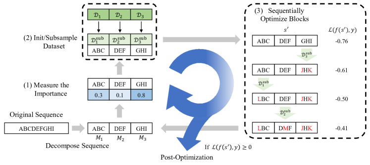
Figure 1: The overall process of BBA. A green arrow with a dataset $\mathcal{D}_{k}^{\text{sub}}$ denotes the Bayesian optimization step for the block $M_{k}$ using $D_{k}^{\text{sub}}$ as the initial dataset.

4 Methods

In this section, we introduce the proposed Blockwise Bayesian Attack (BBA) framework. Instead of optimizing Section 3.1 directly, we divide the optimization into two steps. First, we conduct Bayesian optimization to maximize the black-box function $\mathcal{L}(f_{\theta}(\cdot),y)$ on the attack space $\mathcal{S}\triangleq\prod_{i=0}^{l-1}\mathcal{C}(w_{i})$ until finding an adversarial sequence $s_{\text{adv}}$, which is a feasible solution of Section 3.1. This step can be formulated as

$$\mathop{\mathrm{maximize}}_{s^{\prime}\in\mathcal{S}}~{}\mathcal{L}(f_{\theta}(s^{\prime}),y).$$ (2)

Second, after finding a valid adversarial sequence $s_{\text{adv}}$ that satisfies the attack criterion $\mathcal{L}(f_{\theta}(s_{\text{adv}}),y)\geq 0$, we seek to reduce the Hamming distance of the perturbed sequence from the original input while maintaining the constant feasibility.

Note that Equation 2 is a high-dimensional Bayesian optimization problem on combinatorial search space, especially for datasets consisting of long sequences. However, the number of queries required to obtain good coverage of the input space, which is necessary to find the optimal solution, increases exponentially with respect to the input dimensions due to the curse of dimensionality (shahriari2015taking). This high query complexity is prohibitive for query-efficient adversarial attacks. Furthermore, even in a low-dimensional space, the high computational complexity of training GP models in Bayesian optimization can drastically slow down the runtime of the algorithm as the evaluation history becomes larger. Fitting the GP model requires the matrix inversion of the covariance matrix $K(\hat{X},\hat{X})$, whose computational complexity is $\mathcal{O}(n^{3})$, where $n$ is the number of evaluations so far.

To this end, we first introduce the surrogate model and the parameter fitting method which are suitable for our high-dimensional combinatorial search space. Next, we propose two techniques to deal with the scalability issues that arise from the high query and computational complexity of Bayesian optimization. Lastly, we introduce a post-optimization technique that effectively minimizes the perturbation size of an adversarial sequence.

4.1 Surrogate Model and GP Parameter Fitting

Choosing an appropriate kernel that captures the structure of the high-dimensional combinatorial search space is the key to the success of our GP-based surrogate model. We use a categorical kernel with automatic relevance determination (ARD) to automatically determine the degree to which each input dimension is important (mackay1992bayesian). The kernel has the following form:

$$K^{\text{cate}}(s^{(1)},s^{(2)})=\sigma_{f}^{2}\prod_{i=0}^{l-1}\exp\left(-\frac{\mathbf{1}[w_{i}^{(1)}\neq w_{i}^{(2)}]}{\beta_{i}}\right),$$

where $\sigma_{f}^{2}$ is a signal variance, $\beta_{i}$ is a length-scale parameter corresponding to the relevance of $i$-th element position. This implies that the kernel regards a sequence pair sharing a larger number of elements as a more similar pair. The GP parameter $\beta_{i}$ is estimated by maximizing the posterior probability of the evaluation history under a prior using the gradient descent with Adam optimizer (Adam). More details can be found in LABEL:app:GP.

4.2 Techniques for Scalability

To achieve a scalable Bayesian optimization algorithm, we decompose an input sequence into disjoint blocks of element positions and optimize each block in a sequential fashion for several iterations using data subsampled from the evaluation history corresponding to the block.

4.2.1 Block Decomposition

We divide an input sequence of length $l$ into $\lceil l/m\rceil$ disjoint blocks of length $m$. Each $k$-th block $M_{k}$ consists of consecutive indices $[km,\ldots,(k+1)m-1]$. We sequentially optimize each block for $R$ iterations, rather than updating all element positions concurrently. For each iteration, we set the maximum query budget to $N_{k}$ when optimizing the block $M_{k}$. While the dimension of the attack space $\prod_{i=0}^{l-1}\mathcal{C}(w_{i})$ grows exponentially as $l$ increases, the block decomposition makes the dimension of the search space of each Bayesian optimization step independent of $l$ and upper bounded by $(C_{\text{max}})^{m}$, where $C_{\text{max}}\triangleq\max_{i\in[l]}|\mathcal{C}_{i}|$ is the size of the largest synonym set.

At the start of each iteration, we assign an importance score to each block, which measures how much each block contributes to the objective function value. Then, we sequentially optimize blocks in order of highest importance score for query efficiency. For the first iteration, we set the importance score of each block to the change in the objective function value after deleting the block. For the remaining iterations, we reassign the importance score to each block $M_{k}$ by summing the inverses of the length-scale parameters that correspond to the element positions in $M_{k}$, i.e., $\sum_{i\in M_{k}}1/\beta_{i}$.

Algorithm 1 SoD$(\mathcal{D},N)$, Subset of Data method

1:  Input: The evaluation history $\mathcal{D}$, the size of subsamples $N$.

2:  if $|\mathcal{D}|<N$ then

3:     Return $\mathcal{D}$.

4:  end if

5:  Initialize the dataset $\mathcal{D}_{\text{sub}}\leftarrow\{s_{0}\}$ where $s_{0}$ is randomly sampled from $\mathcal{D}$.

6:  while $|\mathcal{D}_{\text{sub}}|<N$ do

7:     Select the farthest sequence. $s_{\text{far}}\leftarrow\mathop{\rm argmax}_{s\in\mathcal{D}\setminus\mathcal{D}_{\text{sub}}}[\min_{s^{\prime}\in\mathcal{D}_{\text{sub}}}d(s,s^{\prime})]$

8:     Update the dataset $\mathcal{D}_{\text{sub}}\leftarrow\mathcal{D}_{\text{sub}}\cup\{s_{\text{far}}\}$.

9:  end while

10:  Return $\mathcal{D}_{\text{sub}}$.

Algorithm 2 PostOpt$(s,s_{\text{adv}},\mathcal{D}_{\text{sub}},N_{\text{post}},N_{b})$

1:  Input: The original sequence $s$, an adversarial sequence $s_{\text{adv}}$, the evaluation dataset $\mathcal{D}_{\text{sub}}$ subsampled from the evaluation history, the query budget $N_{\text{post}}$, and the batch size $N_{b}$.

2:  Initialize $N_{r}\leftarrow N_{\text{post}}$.

3:  while $N_{r}>0$ do

4:     Fit GP parameters to maximize the posterior probability distribution on $\mathcal{D}_{\text{sub}}$.

5:     Select a batch $B$ of the size $\min(N_{b},N_{r})$ from $\mathcal{B}_{H}(s,d_{H}(s,s_{\text{adv}})-1)\cap\mathcal{B}_{H}(s_{\text{adv}},r)$ according to the acquisition function and the DPP.

6:     Evaluate the batch $\mathcal{D}_{\text{batch}}=\{(s^{\prime},\mathcal{L}(f_{\theta}(s^{\prime}),y)\}_{s^{\prime}\in B}$.

7:     Update the dataset $\mathcal{D}_{\text{sub}}\leftarrow\mathcal{D}_{\text{sub}}\cup\mathcal{D}_{\text{batch}}$.

8:     $N_{r}\leftarrow N_{r}-|\mathcal{D}_{\text{batch}}|$.

9:     if $B$ has an adversarial sequence then

10:        Update $s_{\text{adv}}$ to the best adversarial sequence in $B$.

11:        $N_{r}\leftarrow N_{\text{post}}$.

12:     end if

13:  end while

14:  Return $s_{\text{adv}}$.

4.2.2 History Subsampling

Here, we propose a data subsampling strategy suitable for our block decomposition method. When we optimize a block $M_{k}$, only the elements in $M_{k}$ are updated while the remaining elements are unchanged. Thus, in terms of the block $M_{k}$, all sequences evaluated during the optimization steps for blocks other than $M_{k}$ share the same elements, which do not provide any information on how much $M_{k}$ affects the objective function value. To avoid this redundancy, we consider utilizing only the sequences collected from the previous optimization steps for $M_{k}$ as the evaluation history, denoted by $\mathcal{D}_{k}$, when optimizing $M_{k}$.

On top of the strategy above, we further reduce the computational complexity of Bayesian optimization by subsampling a dataset from the evaluation history and training the GP surrogate model with the reduced dataset. We adopt the Subset of Data (SoD) method with Farthest Point Clustering (FPC) (SOD), a simple and efficient subsampling method widely used in the GP literature. Concretely, we randomly sample an initial sequence from the evaluation history and sequentially select the farthest sequence that maximizes the Hamming distance to the nearest of all sequences picked so far. The overall procedure is shown in Algorithm 1. When optimizing a block $M_{k}$ at each iteration, we select a subset $\mathcal{D}_{k}^{\text{sub}}$ from the evaluation history $\mathcal{D}_{k}$ via the subsampling algorithm above and proceed with the Bayesian optimization step for $M_{k}$ using $\mathcal{D}_{k}^{\text{sub}}$ as the initial dataset for the GP model training.

Here, we simply set the initial subset size to $N_{k}$, which is the same as the maximum query budget when optimizing the block $M_{k}$. Thus, the size of the dataset $\mathcal{D}_{k}^{\text{sub}}$ during a single block optimization step is upper bounded by $\mathcal{O}(N_{k})$. Therefore, we can write the complexity of the GP model fitting step when optimizing a block by $\mathcal{O}((\max_{k}{N_{k}})^{3})$, which is independent of the total number of evaluations, $n$. More details containing the runtime analysis of the overall process can be found in LABEL:app:exp and LABEL:app:RA.

Table 1: Attack results for XLNet-base, BERT-base, and LSTM models on sentence-level classification datasets.

(a) WordNet

Dataset Model Method ASR (%) MR (%) Qrs AG BERT-base PWWS 57.1 18.3 367 BBA 77.4 17.8 217 LSTM PWWS 78.3 16.4 336 BBA 83.2 15.4 190 MR XLNet-base PWWS 83.9 14.4 143 BBA 87.8 14.4 77 BERT-base PWWS 82.0 15.0 143 BBA 88.3 14.6 94 LSTM PWWS 94.2 13.3 132 BBA 94.2 13.0 67

(b) Embedding

Dataset Model Method ASR (%) MR (%) Qrs AG BERT-base TF 84.7 24.9 346 BBA 96.0 18.9 154 LSTM TF 94.9 17.3 228 BBA 98.5 16.6 142 MR XLNet-base TF 95.0 18.0 101 BBA 96.3 16.2 68 BERT-base TF 89.2 20.0 115 BBA 95.7 16.9 67 LSTM TF 98.2 13.6 72 BBA 98.2 13.1 54

(c) HowNet

Dataset Model Method ASR (%) MR (%) Qrs AG BERT-base PSO 67.2 21.2 65860 BBA 70.8 15.5 5176 LSTM PSO 71.0 19.7 44956 BBA 71.9 13.7 3278 MR XLNet-base PSO 91.3 18.6 4504 BBA 91.3 11.7 321 BERT-base PSO 90.9 17.3 6299 BBA 90.9 12.4 403 LSTM PSO 94.4 15.3 2030 BBA 94.4 11.2 138

Table 2: Attack results for BERT-base models on document-level classification datasets.

(a) WordNet

Dataset Method ASR (%) MR (%) Qrs IMDB PWWS 97.6 4.5 1672 BBA 99.6 4.1 449 LSH 96.3 5.3 557 BBA 98.9 4.8 372 Yelp PWWS 94.3 7.6 1036 BBA 99.2 7.4 486 LSH 92.6 9.5 389 BBA 98.8 8.8 271

(b) Embedding

Dataset Method ASR (%) MR (%) Qrs IMDB TF 99.1 8.6 712 BBA 99.6 6.1 339 LSH 98.5 5.0 770 BBA 99.8 4.9 413 Yelp TF 93.5 11.1 461 BBA 99.8 9.6 319 LSH 94.7 8.9 550 BBA 99.8 8.6 403

(c) HowNet

Dataset Method ASR (%) MR (%) Qrs IMDB PSO 100.0 3.8 113343 BBA 100.0 3.3 352 LSH 98.7 3.2 640 BBA 99.8 3.0 411 Yelp PSO 98.8 10.6 86611 BBA 98.8 8.2 283 LSH 93.9 8.0 533 BBA 98.2 7.4 353

4.2.3 Acquisition Maximization Considering Batch Diversity via Determinantal Point Process

We utilize expected improvement as the acquisition function, which is defined as $\mathrm{EI}(x)=\mathrm{E}[\max(g(s)-g^{*}_{\mathcal{D}},0)]$, where $g^{*}_{\mathcal{D}}=\max_{\hat{y}\in\hat{Y}}\hat{y}$ is the largest value evaluated so far.

To further enhance the runtime of the Bayesian optimization algorithm, we evaluate a batch of sequences parallelly in a single round, following the practice in HDBBO. We sample an evaluation batch $B$ via a Determinantal Point Process (DPP), which promotes batch diversity by maximizing the determinant of its posterior variance matrix $\mathrm{Var}(g(B)\mid\mathcal{D})$ (kulesza2012determinantal). Concretely, we first select sequences with top-$T$ acquisition values in the 1-Hamming distance ball $\mathcal{B}_{H}(s^{*}_{\mathcal{D}},1)$ of the best sequence $s^{*}_{\mathcal{D}}$ evaluated so far. Then, we greedily choose $N_{b}$ sequences among the top-$T$ sequences that maximize the determinant. More details can be found in LABEL:app:exp.

4.3 Post-Optimization for Perturbation Reduction

Since we do not consider the perturbation size during the first step of BBA, we conduct a post-optimization step to reduce the perturbation size. To this end, we optimize for a sequence near the current adversarial sequence $s_{\text{adv}}$ that stays adversarial and has a smaller perturbation than $s_{\text{adv}}$. To achieve this, we search an adversarial sequence in a reduced search space $\mathcal{B}_{H}(s,d_{H}(s,s_{\text{adv}})-1)\cap\mathcal{B}_{H}(s_{\text{adv}},r)$, where $r$ controls the exploration size. We also conduct Bayesian optimization for the post-optimization step. We leverage the evaluation history collected during the first step of BBA and subsample an initial dataset for the GP model training from the history. If we find a new adversarial sequence during this step, we replace the current adversarial sequence with the new sequence and repeat the step above until we cannot find a new adversarial sequence using the query budget $N_{\text{post}}$ after the most recent update. The overall post-optimization procedure is summarized in Algorithm 2.

Figure 1 illustrates the overall process of BBA. Please refer to LABEL:alg:main in LABEL:app:mainalg for the more detailed overall algorithm of BBA.

5 Experiments

We evaluate the performance of BBA on text classification, textual entailment, and protein classification tasks. We first provide a brief description of the datasets, victim models, and baseline methods used in the experiments. Then, we report the performance of BBA compared to the baselines. Our implementation is available at https://github.com/snu-mllab/DiscreteBlockBayesAttack.

Figure 2: The cumulative distribution of the number of queries required for the attack methods against a BERT-base model on the Yelp dataset. We use the HowNet based word substitution when comparing our method against LSH.

5.1 Datasets and Victim Models

To demonstrate the wide applicability and effectiveness of BBA, we conduct experiments on various datasets in the NLP and protein domain. In the NLP domain, we use sentence-level text classification datasets (AG’s News, Movie Review), document-level classification datasets (IMDB, Yelp), and textual entailment datasets (MNLI, QNLI) (Yelp_and_AG; MR; IMDB; MNLI; QNLI). In the protein domain, we use an enzyme classification dataset (EC) with 3-level hierarchical multi-labels (EC50). Note that a protein is a sequence of amino acids, each of which is a discrete categorical variable.

We consider multiple types of victim models to attack, including bi-directional word LSTM, ASGD Weight-Dropped LSTM, fine-tuned BERT-base and BERT-large, and fine-tuned XLNet-base and XLNet-large (LSTM; AWD-LSTM; BERT; XLNet). More details on datasets and victim models can be found in LABEL:app:datasets and LABEL:app:models, respectively.

5.2 Baseline Methods

In the NLP domain, we compare the performance of BBA against the state-of-the-art methods such as PWWS, TextFooler, LSH, BAE, and PSO, the first four of which are greedy-based algorithms (PWWS; TextFooler; LSH; BAE; PSO). Note that PWWS, TextFooler, BAE, and PSO have different attack search spaces since they utilize different word substitution methods (WordNet, Embedding, BERT masked language model, and HowNet, respectively) (WordNet; mrkvsic2016counter; HowNet). For a fair comparison, we follow the practice in LSH and compare BBA against each baseline individually under the same attack setting (e.g., word substitution method, query budget) as used in the baseline. We also note that LSH leverages additional attention models, each of which is pre-trained on a different classification dataset. Please refer to LABEL:app:spaces for more details.

For the protein classification task, we compare BBA with TextFooler. To define its attack space, we exploit the experimental exchangeability of amino acids (ExEx), which quantifies the mean effect of exchanging one amino acid to a different amino acid on protein activity, as the measure of semantic similarity. Then, we define a synonym set for each amino acid by thresholding amino acids with the experimental exchangeability and set the attack space to the product of the synonym sets. As in the NLP domain, we compare BBA with the baseline under the same experimental setting as used in the baseline.

5.3 Attack Performance

We quantify the attack performance in terms of three main metrics: attack success rate (ASR), modification rate (MR), and the average number of queries (Qrs). The attack success rate is defined as the rate of successfully finding misclassified sequences from the original sequences that are correctly classified, which directly measures the effectiveness of the attack method. The modification rate is defined as the percentage of modified elements after the attack, averaged over successfully fooled sequences. This rate is formally written by $\mathrm{E}[d_{H}(s,s_{\text{adv}})/\mathrm{len}(s)]$, which quantifies the distortion of the perturbed sequences from the original. The average number of queries, computed over all sequences being attacked, represents the query efficiency of the attack methods.

The main attack results on text classification tasks are summarized in Tables 1(a) and 2(a). The results show that BBA significantly outperforms all the baseline methods in all the evaluation metrics for all datasets and victim models we consider. Figure 2 shows the cumulative distribution of the number of queries required for the attack methods against a BERT-base model on the Yelp dataset. The results show that BBA finds successful adversarial texts using fewer queries than the baseline methods. More experimental results on other target models (BERT-large, XLNet-large), baseline method (BAE), and datasets (MNLI, QNLI) can be found in LABEL:app:add.

Moreover, Table 3 shows that BBA outperforms the baseline method by a large margin for the protein classification task, which shows the general applicability and effectiveness of BBA on multiple domains.

Table 3: Attack results against AWD-LSTM models on the protein classification dataset EC50 level 0, 1, and 2.

Level 0 Level 1 Level 2 Method ASR MR Qrs ASR MR Qrs ASR MR Qrs TF 83.8 3.2 619 85.8 3.0 584 89.6 2.5 538 BBA 99.8 2.9 285 99.8 2.3 293 100.0 2.0 231

For a direct comparison with a baseline, one can compute the MR and Qrs over the texts that both BBA and the baseline method are successful on. Table 4 shows that BBA outperforms PWWS in MR and Qrs on samples that both methods successfully fooled by a larger margin.

Table 4: Attack results on the AG’s News. MR and Qrs of ‘both success’ are averaged over the texts that both PWWS and BBA successfully fooled.

Both success Model Method ASR (%) MR (%) Qrs MR (%) Qrs BERT-base PWWS 57.1 18.3 367 17.8 311 BBA 77.4 17.8 217 14.0 154 LSTM PWWS 78.3 16.4 336 16.1 311 BBA 83.2 15.4 190 14.4 163

5.4 Ablation Studies

5.4.1 The Effect of DPP in Batch Update

To validate the effectiveness of the DPP-based batch update technique, we compare BBA with the greedy-style batch update which chooses the sequences of top-$N_{b}$ acquisition values for the next evaluations. We do not utilize the post-optimization process to isolate the effect of the batch update. Table 5 shows that the batch update with DPP consistently achieves higher attack success rate using fewer queries compared to the greedy-style batch update. Surprisingly, the batch update with DPP achieves higher attack success rate using fewer queries compared to ‘without batch update’ in AG’s News dataset.

Table 5: Attack results of BBA with and without batch update using the WordNet-based word substitution against BERT-base and LSTM models on the sentence-level classification datasets. ‘Top-$N_{b}$’ denotes the greedy-style batch update that chooses sequences of top-$N_{b}$ acquisition values.

BERT-base LSTM Dataset Method ASR (%) Qrs ASR (%) Qrs AG w/o batch 76.1 126 73.5 127 w/ batch, Top-$N_{b}$ 75.9 133 74.3 127 w/ batch, DPP 77.4 124 83.2 86 MR w/o batch 88.5 26 93.9 18 w/ batch, Top-$N_{b}$ 87.1 28 93.6 20 w/ batch, DPP 88.3 25 94.2 17

Table 6: Examples of the original and their adversarial sequences from Yelp and EC50 against BERT-base models.