How You Start Matters for Generalization

Abstract

Characterizing the remarkable generalization properties of over-parameterized neural networks remains an open problem. In this paper, we promote a shift of focus towards initialization rather than neural architecture or (stochastic) gradient descent to explain this implicit regularization. Through a Fourier lens, we derive a general result for the spectral bias of neural networks and show that the generalization of neural networks is heavily tied to their initialization. Further, we empirically solidify the developed theoretical insights using practical, deep networks. Finally, we make a case against the controversial flat-minima conjecture and show that Fourier analysis grants a more reliable framework for understanding the generalization of neural networks.

1 Introduction

Neural networks are often used in the over-parameterized regime, and therefore, have the capacity to converge to many global minima that achieve zero training error. However, converging to such solutions is a non-convex, high-dimensional problem, which is typically intractable to solve. Furthermore, each of these minima may have unique properties that can lead to varying generalization performance, making some solutions preferred than others. Surprisingly, however, it is widely established that when neural networks are trained with gradient-based optimization techniques, they not only converge towards a global minimum, but also are biased towards solutions that exhibit good generalization even without explicit regularization. This mysterious behavior is flagged as the “implicit regularization” of neural networks and remains an open research problem.

To understand implicit regularization, numerous studies have considered simplified settings with restrictive assumptions such as linear networks (Jacot et al., 2018a; Soudry et al., 2018; Wei et al., 2019; Yun et al., 2020; gunasekar2018implicit; Wu et al., 2019), shallow networks (Gunasekar et al., 2018; Ji and Telgarsky, 2019; Ali et al., 2020), wide networks (Jacot et al., 2018b; Mei et al., 2019; Chizat and Bach, 2020; Oymak and Soltanolkotabi, 2019), vanishing initialization (Chizat et al., 2019; Gunasekar et al., 2017; Arora et al., 2019), or infinitesimal learning rates (Ma et al., 2018; Li et al., 2018; Ji and Telgarsky, 2018; Moroshko et al., 2020). Despite different assumptions, most of these works primarily focus on the effect of optimization procedure over the other factors and, at a high level, conclude that gradient-based optimizations guides neural networks toward max-margin solutions for separable data or minimize a notion of weight-norm in regression. While the aforementioned studies yield powerful insights, they lead to rather disconnected views that do not take important factors such as initialization or practical architectures into consideration. As a result, faithful extrapolation of these theoretical conclusions to practical settings becomes problematic.

Our work is an attempt to fill this void. To this end, we show substantial evidence that initialization plays a decisive role in determining the generalization of a neural network. In particular, we demonstrate that even with gradient-based optimization and a deep architecture – networks can converge to solutions with extremely poor generalization properties. We further demonstrate that this result depends on the Fourier spectrum at initialization. It should be noted that our result is not a recapitulation of the well-known observation that bad initialization hampers the convergence of neural networks. Rather, we show that initializing networks such that they have higher energies for higher frequencies leads to solutions that achieve perfect training accuracy, yet succumb to inferior test accuracy. We further reveal that this is a generic property that holds in both classification and regression settings across various architectures.

The roots of our analysis extend to the “spectral bias” (also known as the frequency principle) of neural networks (Xu et al., 2019; Rahaman et al., 2019). Spectral bias is an interesting phenomenon that implies networks tend to learn low frequencies faster, and consequently, tend to fit training data with low frequency functions. However, still there are some critical concerns entailed with existing research. First, studying spectral bias has so far been restricted to neural architectures with traditional activations such as ReLU (Rahaman et al., 2019; Xu et al., 2019), sigmoid (Luo et al., 2019), or tanh (Xu, 2018). Thus, it is intriguing to investigate whether the spectral bias is a universal property that holds across various neural architectures and activation functions. This is important, as it enables the machine learning community to use spectral bias as a tool for investigating implicit regularization more systematically. Second, the question remains whether the spectral bias of a network is a sufficient condition for good generalization. We posit that the answers to these questions can potentially broaden the understanding of implicit regularization of neural networks.

The central objective of this paper aims to shed light on the above questions. To this end, we utilize recently popularized implicit neural networks (Tancik et al., 2020; Ramasinghe and Lucey, 2021) (also referred to as coordinate-based networks) as an initial test-bed. Implicit neural networks are architecturally modified fully-connected networks – using non traditional activations such as Gaussians/sinusoids or positional embedding layers – that can learn high-frequency functions rapidly. In particular, we first demonstrate that implicit neural networks do not always converge to smooth solutions, contradicting mainstream expectations. In resolving this controversial observation, first, we invoke a compact data manifold hypothesis to show that spectral bias is both architecture- and loss-agnostic in a general sense. To our knowledge, this is the most general proof of spectral bias to date in literature. With this in hand, we affirm that the poor generalization of implicit neural networks is linked to the presence of high frequencies at initialization. Similarly, we further show that the implicit regularization of neural networks requires an initial spectrum that is biased towards lower frequencies. We postulate that the remarkable generalization properties of modern neural architectures can be partly attributed to the employment of non-linearities (such as ReLU) that exhibit such spectra upon random initialization. Extending the above analysis, we depict that even ReLU networks, when initialized with a higher frequencies, fail to converge to minima with good generalization properties.

Finally, we investigate the “flat minima conjecture" (that the generalisation capacity of a neural network is determined by the flatness of the minimum to which training has converged) for multiple architectures. We find that the consistency of the conjecture with experiment is architecture-dependent, while the predictions made using a spectral bias approach are consistent across all examined architectures and problems.

Our main contributions are listed below:

• We offer, to our knowledge, the simplest and most general proof of the spectral bias phenomenon in literature. Our result applies to all presently-used neural network architectures (along with a vast space of parameterised models that are not neural networks) in problems satisfying the compact data manifold hypothesis.

• We show that initialization plays a crucial role in governing the implicit regularization of neural networks. Our results advocate for a shift of focus towards initialization in understanding the generalization paradox, which currently revolves around the optimization procedure.

• We conduct experiments in both classification and regression settings. We show that the developed insights are generic across different architectures, non-linearities, and initialization schemes. Our experiments include practical, deep networks, in contrast to many existing related works.

• We present (empirical) counter-evidence against the flat minima conjecture and show that 1) SGD is not always biased towards flat minima and 2) flat minima do not always correlate with better generalization.

2 Related Works

Implicit regularization

Mathematically characterizing implicit regularization of neural networks is at the heart of understanding deep learning. This intriguing phenomenon received increasing attention from the machine learning community after the seminal work by Zhang et al. (2016), in which they showed that deep models, despite having the capacity to fit even random data, demonstrate remarkable generalization properties. Since then, an extensive body of works have tried to characterize implicit regularization through various lenses including training dynamics (Advani et al., 2020; Gidel et al., 2019; Lampinen and Ganguli, 2018; Goldt et al., 2019; Arora et al., 2019), flat minima conjecture (Keskar et al., 2016; Jastrzębski et al., 2017; Wu et al., 2018; Simsekli et al., 2019; Mulayoff and Michaeli, 2020), statistical properties of data (Brutzkus and Globerson, 2020), architectural aspects such as skip connections He et al. (2020); Huang et al. (2020), and matrix factorization Gunasekar et al. (2017); Arora et al. (2019); Razin et al. (2021). At a high-level, these works show that deep models implicitly minimize a form of weight norms, regularize derivatives of the outputs, or analogously, maximize a notion of margin between output classes. However, the center of attention of (almost all) these works is the bias induced by the optimization (SGD) methods. In contrast, we show that while SGD induces a crucial bias, (less highlighted) initialization also plays an important role. Notably, Min et al. (2021) recently discussed the role of initialization in the convergence and implicit bias of neural networks. They showed that the rate of convergence of a neural network depends on the level of imbalance of the initialization. Their setting, however, only considered single-hidden-layer linear networks under the square loss. In contrast, we offer richer insights and consider a broader and more practical setting in our work by using deeper, practical networks.

Spectral bias

Neural networks tend to learn low frequencies faster. To the best of our knowledge, this peculiar behavior was first systematically demonstrated on ReLU networks by Xu et al. (2019) and Rahaman et al. (2019) in independent studies, and a subsequent theoretical work showed that shallow networks with Tanh activations (Xu, 2018) also admit the same bias. Several recent works have also attempted to characterize the spectral bias of neural networks in different training phases and under various (relatively restrictive) architectural assumptions Luo et al. (2019); Zhang et al. (2019); Luo et al. (2020). Perhaps, the insights developed by Zhang et al. (2019) and Luo et al. (2020) are more closely aligned with some of the conclusions of our work, in which they showed that shallow ReLU networks with infinite width converge to solutions by minimally changing the initial Fourier spectrum.

Implicit neural networks

Implicit neural networks are a class of fully connected networks that were recently popularized by the seminal work of Mildenhall et al. (2020). Implicit neural networks either use non-traditional activation functions (Gaussian (Ramasinghe and Lucey, 2021) or Sinusoid (Sitzmann et al., 2020)) or positional embedding layers (Tancik et al., 2020; Zheng et al., 2021). The key difference between implicit neural networks and conventional fully connected networks is that the former can learn high frequency functions more effectively and, thus, can encode natural signals with higher fidelity. Owing to this unique ability, implicit neural networks have penetrated many tasks in computer vision such as texture generation (Henzler et al., 2020; Oechsle et al., 2019; Henzler et al., 2020; Xiang et al., 2021), shape representation (Chen and Zhang, 2019; Deng et al., 2020; Tiwari et al., 2021; Genova et al., 2020; Basher et al., 2021; Mu et al., 2021; Park et al., 2019), and novel view synthesis (Mildenhall et al., 2020; Niemeyer et al., 2020; Saito et al., 2019; Sitzmann et al., 2019; Yu et al., 2021; Pumarola et al., 2021; Rebain et al., 2021; Martin-Brualla et al., 2021; Wang et al., 2021; Park et al., 2021).

3 Generalization and Fourier spectrum of neural networks

Generalization of neural networks

Consider a set of training data $\{\mathbf{x}_{i},\mathbf{y}_{i}\}_{i=1}^{N}$ sampled from a distribution $\mathbb{D}$. Given a new set $\{\bar{\mathbf{x}},\bar{\mathbf{y}}\}\sim\mathbb{D}$, where a neural network $f$ only observes $\{\bar{\mathbf{x}}\}$, the goal is to learn a function such that $f(\bar{\mathbf{x}})\approx\bar{\mathbf{y}}$. Since $\mathbb{D}$ is unknown, the network tries to learn a function that minimizes an expected cost $\mathbb{E}[\mathcal{L}(f(\mathbf{x}_{i}),\mathbf{y}_{i})]$ over the training data, where $\mathcal{L}$ is a suitable loss function. After training, if the network acts as a good estimator $f:\bar{\mathbf{x}}\to\bar{\mathbf{y}}$, we say that $f$ generalizes well. In classification, usually, a variant of the cross-entropy loss is chosen as $\mathcal{L}$, and in regression, $\ell_{1}$ or $\ell_{2}$ loss is chosen. It should be noted that generalization is entirely a function of $\mathbb{D}$ and thus, cannot be measured without priors on $\mathbb{D}$. In image classification, for instance, a held-out set of validation/testing data is used to as prior on $\mathbb{D}$ to measure the generalization performance. In regression, due to the infinite sampling precision of both input and output spaces, the use of such held-out data becomes less meaningful. Thus, a more practical method of measuring the generalization in a regression setting, at least in an engineering sense, is to measure the “smoothness” of interpolation between training data. That is, we say that a network generalizes well if its output is smooth while fitting the training data.

Smooth interpolations and the Fourier spectrum

In machine learning and statistics, a “smooth” signal is typically considered a signal with bounded higher-order derivatives. This interpretation stems from the fact that, in practice, noise causes large derivatives and, thus, suppressing higher-order derivatives is equivalent to suppressing noise in a signal, leading to better generalization. A widely used approach to obtain a smooth output signal is regularizing the second-order derivatives. For instance, in spline regression, a weighted sum of second-order derivatives and the square loss is minimized to achieve better generalization (Reinsch, 1967; Craven and Wahba, 1978; Kimeldorf and Wahba, 1970). Interestingly, Heiss et al. (2019), showed that shallow ReLU networks, when initialized randomly, implicitly regularize the second-order derivatives of the output over a broad class of loss functional, leading to better generalization. Next we show that minimizing the second-order derivatives of a signal is equivalent to minimizing the power of higher frequencies of that particular signal. Consider an absolutely integrable function $g(x)$ and its Fourier transform $\hat{g}(x)$. Then,

$$g(x)-\int_{-\infty}^{\infty}\hat{g}(k)e^{2\pi jkx}dk$$

$$\bigg{|}\frac{d^{2}g(x)}{dx^{2}}\bigg{|}=\lvert 4\pi^{2}\int_{-\infty}^{\infty}k^{2}\hat{g}(k)e^{2\pi jkx}dk\rvert\leq|4\pi^{2}|\int_{-\infty}^{\infty}|k^{2}\hat{g}(k)|dk$$

Therefore, suppressing the higher frequencies of the Fourier spectrum $\hat{g}(k)$ of a signal reduces the upperbound on the magnitude of the second-order derivatives of that particular signal.

Fourier spectrum of a neural network

To any integrable function $f:\mathbb{R}^{d}\rightarrow\mathbb{R}$ is associated its Fourier transform, given by the formula $\mathcal{F}[f](\mathbf{k}):=\int e^{-i\mathbf{k}\cdot\mathbf{x}}f(\mathbf{x})\,d\mathbf{x}$ Grafakos (2008). In particular, a scalar-valued neural network defines a function $f_{\theta}:\mathbb{R}^{d}\rightarrow\mathbb{R}$, whose Fourier transform makes sense provided $f_{\theta}$ is integrable. We will mollify (set to zero outside of some set) $f_{\theta}$ to take into account data locality, which guarantees integrability. The Fourier transform of a vector-valued network is defined by taking the Fourier transform of each of its component functions.

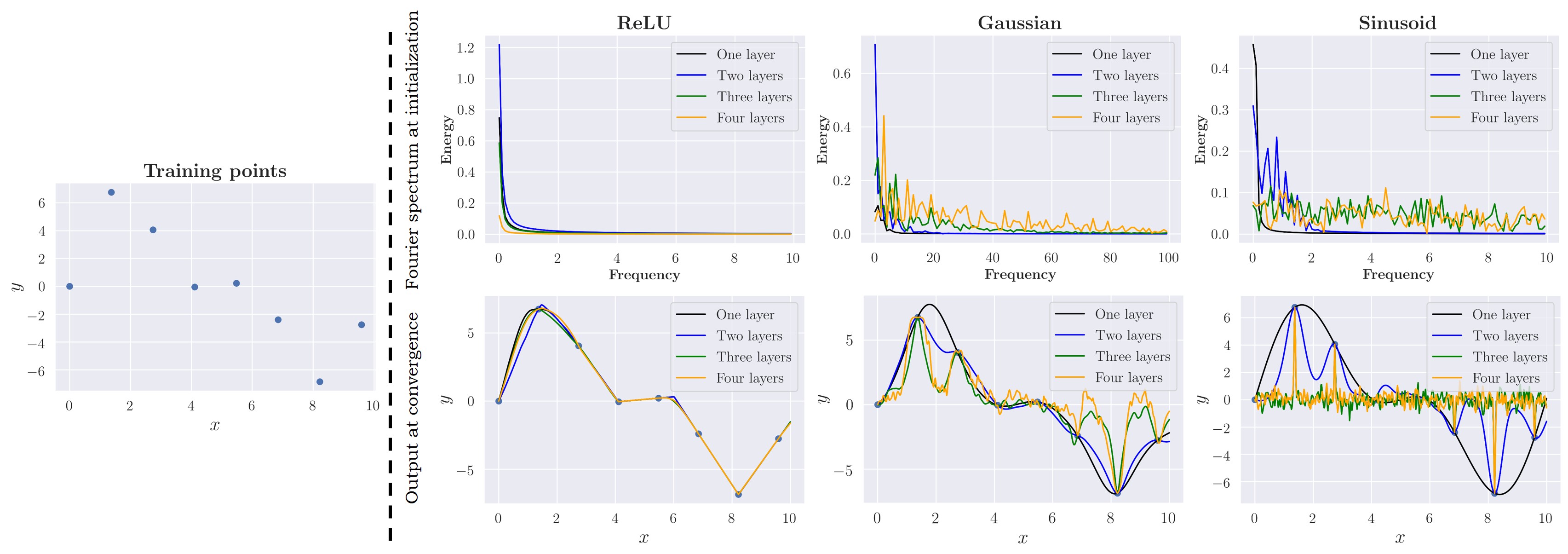
Figure 1: Implicit neural networks are not implicitly regularized. The ReLU network keeps converging to smooth solutions despite the increasing depth. In contrast, Gaussian and sinusoidal networks converge to increasingly erratic solutions as the depth is increased. Interestingly, note that the Gaussian and sinusoidal networks add higher frequencies to the spectrum at initialization as the depth is increased, in contrast to the ReLU network.

4 Implicit neural networks do not always generalize well

In this section, we compare implicit neural networks against conventional ReLU networks in regression, and show that the former do not always generalize well. The experiments are described in detail below.

Experiment 1:

We utilize fully-connected networks with three types of activation functions: 1) ReLU, 2) Gaussian, and 3) Sinusoidal. We sample $8$ sparse points from the signal $3\mathrm{sin}(0.4\pi x)+5\mathrm{sin}(0.2\pi x)$ and regress them using networks across varying depths. As depicted in Fig. 1, when more capacity is added to the ReLU network via hidden layers, the network keeps converging to a smooth solution as expected. In contrast, Gaussian and Sinusoidal networks showcase worsening interpolations, contradicting the mainstream expectations of implicit regularization. Interestingly, it can be observed that sinusoidal and Gaussian networks add more energy to higher frequencies at initialization as more layers are added. In contrast, ReLU networks tend to have a highly biased spectrum towards lower frequencies irrespective of the depth. All the networks are randomly initialized using Xavier initialization (Glorot and Bengio, 2010). We use SGD to optimize the networks with a learning rate of $1\times 10^{-4}$. The networks consist of $256$ neurons in each hidden layer.

Experiment 1 concludes that even with SGD as the optimization algorithm, not all types of networks are implicitly regularized. Instead, the results hint that the initial Fourier spectrum impacts the generalization performance of a neural network, and the network architecture (activation) plays a crucial role in determining the spectrum. In the upcoming sections, we dig deeper into these insights.

5 The universality of spectral bias

Sec. 4 showed that networks with higher frequencies at initialization tend to exhibit poor generalization. However, it is worth investigating if there is indeed a causal link between the two. Intuitively, spectral bias allows us to speculate such a link. That is, one can speculate that the non-smooth interpolations are a result of unwanted residual frequencies after the convergence of lower frequencies. Continuing this line of thought, we present a general proof of the spectral bias, and show that spectral bias is a universal phenomenon that exists in any parameterized function (which includes the class of all neural networks), given that they are trained with gradient-based optimization methods.

Let $f:\mathbb{R}^{p}\times\mathbb{R}^{d}\rightarrow\mathbb{R}$ be a parameterised family $\theta\mapsto f_{\theta}$ of continuous functions $\mathbb{R}^{d}\rightarrow\mathbb{R}$. We assume that the map $(\theta,x)\mapsto f_{\theta}(x)$ is differentiable almost everywhere, and that the restriction of the (almost everywhere-defined) map $x\mapsto D_{\theta}f_{\theta}(x)$ is bounded over any compact set. This setting includes all presently used neural network architectures, with activation functions constrained only to be differentiable almost everywhere.

We care only about the behaviour of $f_{\theta}$ in a neighbourhood of the data. We invoke the compact data manifold hypothesis: that the entire data manifold is contained in some compact neighbourhood $K$. Let $g_{\theta}$ be the extension by zero of $f_{\theta}$ outside of $K$, i.e.

$$g_{\theta}(x):=\begin{cases}f_{\theta}(x)&\text{ if $x\in K$},\\ 0&\text{ otherwise}\end{cases}$$ (1)

Thus $g_{\theta}$ has compact support $K$ and is continuous on $K$ since $f_{\theta}$ is continuous globally. It follows that $g_{\theta}$ is in $L^{1}(\mathbb{R}^{d})$. It follows from the Riemann-Lebesgue lemma (Grafakos, 2008, Proposition 2.2.17) that the Fourier transform $\mathcal{F}[g_{\theta}]$ of $g_{\theta}$ vanishes at infinity. The next theorem shows that the same is true of the change $\frac{d}{dt}[g_{\theta(t)}]$ during training, yielding the first completely general proof of the spectral bias.

Theorem 5.1 (The spectral bias of differentiably parameterised models).

Let $c:\mathbb{R}\times\mathbb{R}\rightarrow\mathbb{R}$ be any differentiable cost function, and let $\{x_{i}\}_{i=1}^{n}$ be a training set drawn from the data manifold, with corresponding target values $\{y_{i}\}_{i=1}^{n}$. Assume that the parameterised function $\theta\mapsto g_{\theta}$ is trained according to almost-everywhere-defined gradient flow:

$$\frac{d}{dt}g_{\theta(t)}(x)=-\frac{1}{n}\sum_{i=1}^{n}\mathcal{K}(\theta(t),x,x_{i})\nabla c(g_{\theta(t)}(x_{i}),y_{i}),$$ (2)

where

$$\mathcal{K}(\theta,x,x^{\prime}):=D_{\theta}g_{\theta}(x)\,D_{\theta}g_{\theta}(x^{\prime})^{T}$$ (3)

is the tangent kernel Jacot et al. (2018a) defined by $g_{\theta}$. Then the Fourier transform $\mathcal{F}[g_{\theta(t)}]$ evolves according to the differential equation

$$\frac{d}{dt}\mathcal{F}[g_{\theta(t)}](\xi)=-\frac{1}{n}\sum_{i=1}^{n}\int_{x\in\mathbb{R}^{d}}e^{-ix\cdot\xi}\mathcal{K}(\theta(t),x,x_{i})\nabla c(g_{\theta(t)}(x_{i}),y_{i})\,dx.$$ (4)

Moreover, $\frac{d}{dt}\mathcal{F}[g_{\theta(t)}]$ vanishes at infinity: $\big{|}\frac{d}{dt}\mathcal{F}[g_{\theta(t)}](\xi)\big{|}\rightarrow 0$ as $\|\xi\|\rightarrow\infty$.

Two remarks are in order regarding the antecedents of Theorem 5.1.

Remark 5.2.

Our use of the tangent kernel in characterising the dynamics of gradient flow are inspired by the seminal work of Jacot et al. (2018a), which is well-known for hypothesising infinite width for several of its results. In fact, the tangent kernel governs gradient flow dynamics independently of any architectural assumptions (beyond the stated differentiability assumption), and in particular, Theorem 5.1 does not require an assumption of infinite width in order to use the tangent kernel. The infinite width hypothesis is invoked in Jacot et al. (2018a) specifically to give a simple proof of evolution towards a global minimum. We do not attempt any such proof and so do not require the infinite width hypothesis.

Remark 5.3.

Our second remark concerns previous proofs of the frequency principle (Zhang et al., 2019; Luo et al., 2020), wherein it was deemed necessary to make simplifying assumptions such as limited depth and infinite width. With these assumptions the authors are able to analytically compute decay rates for the spectral bias. These works also do not take into account the structure of the data. An alternative, more general approach using Sobolev space theory is taken in Luo et al. (2019), wherein the data distribution is accounted for. While Luo et al. (2019) also gives explicit decay rates, the proofs are relatively involved and are only given for chain network architectures. In contrast, we abstract away all detail concerning model architecture beyond minimal regularity assumptions that hold for all presently used neural network models, thereby exhibiting the spectral bias to hold generically for parameterised models, greatly simplifying its proof.

Experiement 2: The goal of this experiment is to (partially) empirically validate the above theoretical conclusions. To this end, we use ReLU, Gaussian, and sinusoid networks. We train the networks on densely sampled points from $g(x)=\sum_{n=1}^{6}\mathrm{sin}(10\pi nx)$. While training, we visualize the convergence of frequency indices of all the networks (Fig. 2). As Theorem 5.1 predicted, all three types of networks exhibit spectral bias. Note that the convergence-decay rates differ across network-types and initialization schemes, which also has an impact on generalization (see Appendix).

In the next section, we show that the initialization plays a key role in generalization and the widely-observed good generalization properties of ReLU networks are merely a consequence of them having biased initial spectra (towards lower frequencies), upon random initialization.

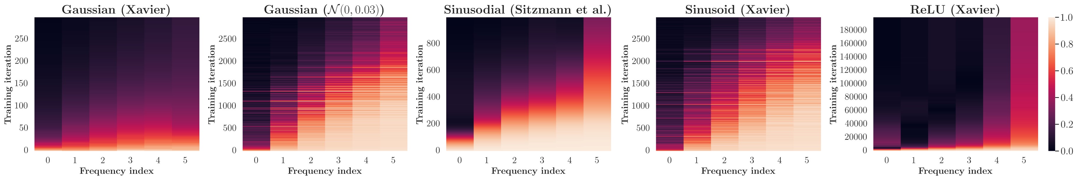
Figure 2: Spectral bias applies to different network types and initialization schemes. We measure the convergence of each frequency index as the training progresses. The colors indicate the difference between the ground truth and the predicted frequencies at each index. Xavier and Sitzmann are the initialization schemes proposed by Glorot and Bengio (2010) and Sitzmann et al. (2020), respectively. Note that the convergence-decay rates of frequencies varies across network types and initialization schemes.

6 ReLU networks do not always generalize well

In this section, we show that the initial Fourier spectrum plays a decisive role in governing the implicit regularization of a neural network. Notably, we show that even ReLU networks (which are commonly expected to regularize well) do not always converge to smooth solutions despite training with SGD.

Experiment 3a:

We investigate and analyze the effect of the initial Fourier spectrum on generalization. First, we sample a signal $\mathrm{sin}(\pi x)$ with a step size of $1$. Thus, the lowest frequency signal that can fit this set of training points is $\mathrm{sin}(\pi x)$ (Nyquist-Shannon sampling theorem). Then, we randomly initialize a ReLU network using Xavier initialization, so that its initial Fourier spectrum does not contain significant energies above the frequency index $k=0.5$ (which corresponds to the lowest frequency solution). After training the network over the training points, the network converges to the lowest frequency solution, i.e., $\mathrm{sin}(\pi x)$.

Experiment 3b:

We utilize the same training points used in Experiment 4a. However, in this instance, we pre-train the ReLU network on a signal $\mathrm{sin}(10\pi x)$. Note that at this instance, the Fourier spectrum of the network has a spike at $k=5$, which is above $k=0.5$. Then, starting from these pre-trained weights, we train the network on the training points.

Experiment 3c:

We initialize a Gaussian network with Xavier initialization, so that it contains frequencies above $k=0.5$. Then, starting from these weights, we train the model on the above training points.

Experiment 3d:

We initialize a Gaussian network with a random weight distribution $\mathcal{N}(0,0.03)$ such that it does not contain frequencies above $k=0.5$. Then, starting from these weights, we train the model on the training points used in the above experiments.

Fig. 3 visualizes the results. As illustrated, when the spectrum of the ReLU network does not contain frequencies higher than $k=0.5$, the final spectrum of the network matches with the lowest frequency solution. In contrast, when the initial spectrum of the ReLU network contains frequencies higher than $k=0.5$, the network adds a spike at $k=0.5$, but leaves the high-frequency spike untouched as the network has already reached zero train error. This results in a non-smooth (poorly generalized) solution. Interestingly, observe that Gaussian networks also can generalize well if the initial spectrum does not contain higher frequencies. It is vital to note that, however, the convergence-decay rates of frequencies also play an important role. For instance, if the convergence-decay rate is low, higher frequencies begin to get affected before the lower frequencies are converged, which can lead to non-smooth solutions (see Appendix). In the next section, we investigate the effect of having high bandwidth spectra at initialization in classification, using popular deep networks.

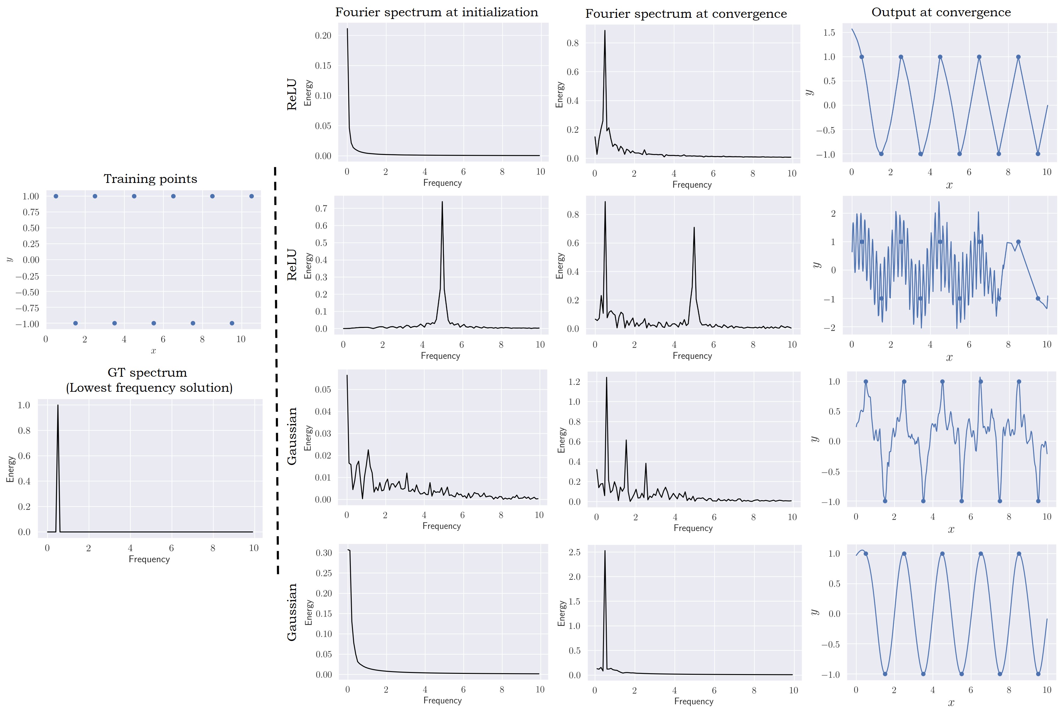
Figure 3: Left block shows sparsely sampled training points from $\mathrm{sin}(\pi x)$ and the corresponding lowest frequency solution that fits the training data. Right block compares generalization corresponding to different networks and initializations. Top row: The ReLU network tries to converge to a solution by changing low frequencies at a faster rate due to spectral bias. Consequently, when initialized with no high frequencies, the network ends up converging to the lowest frequency (hence smooth) solution for the training points. Second row: ReLU networks do not always generalize well. If higher frequencies (than the lowest frequency solution) exist at initialization, ReLU networks reach a solution manipulating only the lower frequencies, resulting in bad interpolations. Third row: Same behavior is demonstrated with a Gaussian network. Fourth row: Gaussian networks can generalize well if initialized properly. Since the network does not contain high frequencies at initialization, it is possible for the network to converge to the lowest frequency solution.

7 Generalization of deep networks in classification

Sec. 5 affirmed that the spectral bias holds for any parameterized model trained using gradient descent. Thus, it is intriguing to explore whether the practical insights we developed thus far extrapolate to popular deep networks that are ubiquitously used. However, for deep networks with high-dimensional inputs (e.g., images), high-bandwidth initialization becomes less straightforward. For instance, consider a network that consumes high dimensional inputs $\mathbf{x}=(x_{1},x_{2},\dots,x_{n})$. Then, one can hope to directly extend the one dimensional technique we used and train the network on the supervisory signal $\mathrm{sin}(wx_{1})\times\mathrm{sin}(wx_{2})\times\dots\times\mathrm{sin}(wx_{n})$. Nevertheless, it is easy to show that in this case, as the dimension of the input grows, the target signal converges to zero. Therefore, we opt for an alternative method and pre-train the models on random labels to obtain higher bandwidths (see Appendix for a discussion).

Experiment 4

We use $9$ popular models for this experiment: VGG16, VGG11, AlexNet, EfficientNet, DenseNet, ResNet-50, ResNet-18, SENet, and ConvMixer. In the first setting, we initialize the models with random weights, train them on the train splits of the datasets, and measure the test accuracy on the test splits. In the next setting, we first pre-train the models on the train split with randomly shuffled labels. Then, starting from the pre-trained weights, we train the models on the train splits of datasets with correct labels and compute the test accuracy on the test splits. The results are depicted in Table 1.

Recall that the pre-trained models on random labels yield higher initial bandwidths compared to randomly initialized models. As evident from the results, starting from a higher bandwidth hinders good generalization, validating our previous conclusions. The test accuracies of some models under random weight initialization (Table 1) are slightly lower than the benchmark results reported in the literature. This is because, following Zhang et al. (2016), we treat data augmentation as an explicit regularization technique and do not use it. In contrast to Zhang et al. (2016), however, we consider dropout and batch normalization as architectural aspects and keep them.

CIFAR10
Model	Random initialization		High B/W initialization
	Train accuracy	Test accuracy	Train accuracy	Test accuracy
VGG11 (Simonyan and Zisserman, 2014)	$100\%$	$84.33\pm 0.49\%$	$100\%$	$71.94\pm 0.71\%$
VGG16 (Simonyan and Zisserman, 2014)	$100\%$	$88.24\pm 0.12\%$	$100\%$	$71.55\pm 0.79$%
AlexNet (Krizhevsky, 2014)	$100\%$	$80.11\pm 1.13\%$	$100\%$	$51.31\pm 0.61\%$
EfficientNet (Tan and Le, 2019)	$100\%$	$76.78\pm 0.57\%$	$100\%$	$61.38\pm 0.46\%$
DenseNet (Huang et al., 2017)	$100\%$	$86.69\pm 0.02\%$	$100\%$	$80.86\pm 0.01\%$
ResNet-18 He et al. (2016)	$100\%$	$82.44\pm 0.15\%$	$100\%$	$68.99\pm 0.62\%$
ResNet-50 He et al. (2016)	$100\%$	$87.18\pm 0.21\%$	$100\%$	$62.72\pm 0.47\%$
SENet (Hu et al., 2018)	$100\%$	$86.31\pm 0.30\%$	$100\%$	$71.20\pm 0.35\%$
ConvMixer (Trockman and Kolter, 2022)	$100\%$	$86.72\pm 0.97\%$	$100\%$	$49.33\pm 0.78\%$
CIFAR100
Model	Random initialization		High B/W initialization
	Train accuracy	Test accuracy	Train accuracy	Test accuracy
VGG11	$100\%$	$54.03\pm 0.71\%$	$100\%$	$41.88\pm 0.94\%$
VGG16	$100\%$	$56.86\pm 0.68\%$	$100\%$	$36.27\pm 1.92\%$
AlexNet	$100\%$	$53.12\pm 1.01\%$	$100\%$	$41.44\pm 1.21\%$
EfficientNet	$100\%$	$43.15\pm 0.58\%$	$100\%$	$26.83\pm 0.89\%$
DenseNet.	$100\%$	$57.76\pm 0.24\%$	$100\%$	$46.56\pm 0.41\%$
ResNet-18	$100\%$	$52.14\pm 0.61\%$	$100\%$	$41.98\pm 0.59\%$
ResNet-50	$100\%$	$54.42\pm 0.78\%$	$100\%$	$30.56\pm 0.58\%$
SENet	$100\%$	$58.64\pm 0.25\%$	$100\%$	$51.56\pm 0.77\%$
ConvMixer	$100\%$	$61.20\pm 0.24\%$	$100\%$	$26.35\pm 0.99\%$
Tiny ImageNet
Model	Random initialization		High B/W initialization
	Train accuracy	Test accuracy	Train accuracy	Test accuracy
VGG11	$100\%$	$38.87\pm 0.41\%$	$100\%$	$27.99\pm 0.73\%$
VGG16	$100\%$	$40.95\pm 0.61\%$	$100\%$	$21.77\pm 0.85\%$
AlexNet	$100\%$	$35.56\pm 0.55\%$	$100\%$	$21.94\pm 1.66\%$
EfficientNet	$100\%$	$33.39\pm 0.42\%$	$100\%$	$18.19\pm 0.92\%$
DenseNet	$100\%$	$48.86\pm 0.35\%$	$100\%$	$28.23\pm 0.27\%$
ResNet-18	$100\%$	$43.58\pm 1.21\%$	$100\%$	$26.73\pm 0.63\%$
ResNet-50	$100\%$	$43.33\pm 1.43\%$	$100\%$	$28.08\pm 0.61\%$
SENet	$100\%$	$28.27\pm 1.33\%$	$100\%$	$24.03\pm 0.29\%$
ConvMixer	$100\%$	$45.38\pm 0.88\%$	$100\%$	$27.77\pm 0.28\%$

Table 1: Generalization of deep networks in classification (accuracy $\pm$ std.). When the models are initialized with higher bandwidths (pre-trained on random labels), the test accuracy drops. This pattern is consistent across various architectures and datasets. We do not use data augmentation in these experiments and each model is run for five times in each setting.

8 A case against the flat minima conjecture

The flat minima conjecture speculates that the generalisation capacity of a network is related to loss landscape geometry. Simply put, the flat minima conjecture postulates that – for some definition of the flatness of the loss landscape – flat minima lead to better generalization (but not vice-versa (Dinh, 2017)). Next, we show that while this conjecture is consistent with the evidence for ReLU networks, it is falsified by Gaussian networks.

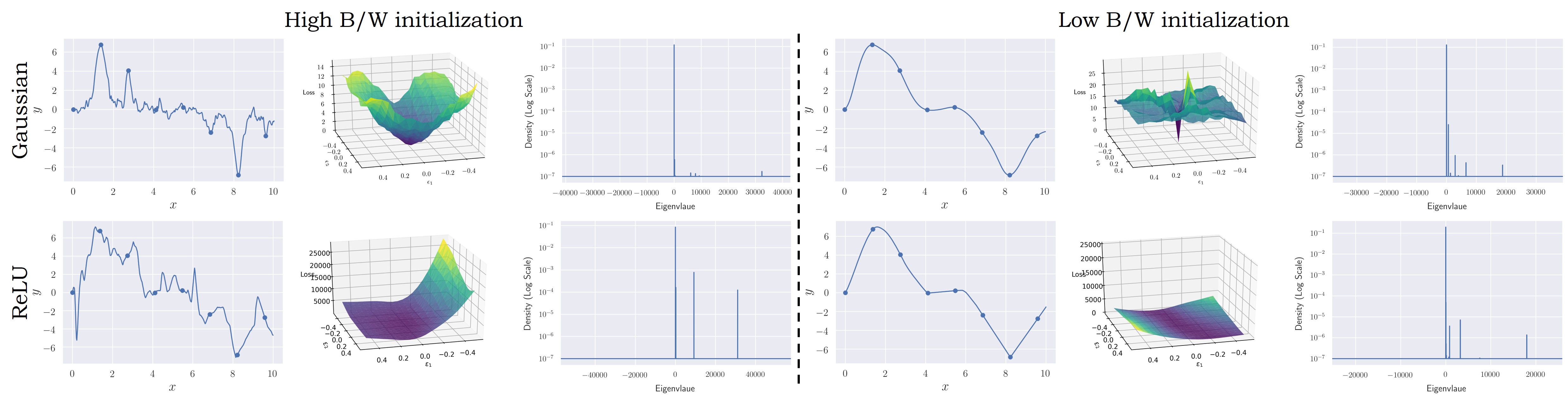
Figure 4: Flat minima conjecture does not always hold. The left block and the right block correspond to high bandwidth and low bandwidth initializations, respectively. In each block, from the left column, the interpolations, loss landscapes, and the eigenvalue distribution of the loss-Hessian are illustrated. The loss landscapes are plotted along with the directions of the two largest eigenvalues. As depicted, while our results for the ReLU network are consistent with the conjecture, the Gaussian network behaves in the opposite manner. For more detailed quantitative results, see Table 2.

Experiment 5

We sample four random variables $w_{1},w_{2}\sim U(0.01,1),a_{1},a_{2}\sim U(1,10)$ and define $20$ signals using the sampled variables as $a_{1}\mathrm{sin}(2\pi w_{1}x)+a_{2}\mathrm{sin}(2\pi w_{2}x)$. Then, we sample $8$ equidistant samples between $0$ and $10$, and use them as the training points to train models. We use Gaussian and ReLU networks for this experiment in two settings. In the first setting, we initialize the ReLU network using Xavier initialization and the Gaussian networks with $\mathcal{N}(0,0.03)$. In this setting, both the networks are able to interpolate the points smoothly. In the other setting, we initialize the ReLU network by pre-training it on $\mathrm{sin}(6\pi x)$ and the Gaussian network with Xavier initialization. In this scenario, both networks demonstrate non-smooth interpolations due to initial high bandwidth. At convergence, we compute the hessian of the loss with respect to the parameters and then compute the eigenvalues and the trace of the hessian. The results are shown in Fig. 4 and Table 2. As evident, the behavior of the Gaussian network is not consistent with the flat minima conjecture. Thus, we advocate that the spectral bias provides a more reliable framework for investigating the generalization of neural networks.

Model	Initialization	Hessian trace	$\mathbb{E}[\epsilon]$	Spectral norm
ReLU	High B/W	$134213.36$	$0.95$	$257875.23$
ReLU	Low B/W	$31110.73$	$0.04$	$49781.58$
Gaussian	High B/W	$40478.82$	$0.21$	$12596.89$
Gaussian	Low B/W	$59447.46$	$0.32$	$26519.66$

Table 2: The trace, expected eigenvalue ($\mathbb{E}[\epsilon)$], and the spectral norm of the loss-Hessian are shown (averaged over $20$ signals). Higher values indicate a sharper minimum. As illustrated, while the ReLU network obeys the flat minima conjecture, the Gaussian network behaves oppositely.

9 Conclusion

In this paper, we focus on the effect of initialization on the implicit generalization of neural networks. In particular, we reveal that the Fourier spectrum of the network at initialization has a significant impact on the generalization gap. Moreover, we offer evidence against the flat minima conjecture and show that the correlation between the flatness of the minima and the generalization can be architecture-dependent. We empirically validate the generality of our insights across diverse, practical settings.

Checklist

1. For all authors…

   1. Do the main claims made in the abstract and introduction accurately reflect the paper’s contributions and scope? [Yes]

   2. Did you describe the limitations of your work? [Yes]

   3. Did you discuss any potential negative societal impacts of your work? [N/A]

   4. Have you read the ethics review guidelines and ensured that your paper conforms to them? [Yes]

2. If you are including theoretical results…

   1. Did you state the full set of assumptions of all theoretical results? [Yes]

   2. Did you include complete proofs of all theoretical results? [Yes]

3. If you ran experiments…

   1. Did you include the code, data, and instructions needed to reproduce the main experimental results (either in the supplemental material or as a URL)? [No]

   2. Did you specify all the training details (e.g., data splits, hyperparameters, how they were chosen)? [Yes]

   3. Did you report error bars (e.g., with respect to the random seed after running experiments multiple times)? [N/A]

   4. Did you include the total amount of compute and the type of resources used (e.g., type of GPUs, internal cluster, or cloud provider)? [No]

4. If you are using existing assets (e.g., code, data, models) or curating/releasing new assets…

   1. If your work uses existing assets, did you cite the creators? [Yes]

   2. Did you mention the license of the assets? [N/A]

   3. Did you include any new assets either in the supplemental material or as a URL? [N/A]

   4. Did you discuss whether and how consent was obtained from people whose data you’re using/curating? [N/A]

   5. Did you discuss whether the data you are using/curating contains personally identifiable information or offensive content? [N/A]

5. If you used crowdsourcing or conducted research with human subjects…

   1. Did you include the full text of instructions given to participants and screenshots, if applicable? [N/A]

   2. Did you describe any potential participant risks, with links to Institutional Review Board (IRB) approvals, if applicable? [N/A]

   3. Did you include the estimated hourly wage paid to participants and the total amount spent on participant compensation? [N/A]

Appendix A Appendix

A.1 Proof of Theorem 5.1

Proof.

The evolution equation for $\mathcal{F}[g_{\theta(t)}]$ follows easily from the Liebniz integral rule:

$$\frac{d}{dt}\mathcal{F}[g_{\theta(t)}]=\mathcal{F}\bigg{[}\frac{d}{dt}g_{\theta(t)}\bigg{]}.$$

Now, $\mathcal{K}$ is nothing other than the extension of the tangent kernel associated to $f_{\theta}$ by zero outside of the compact neighbourhood $K$ of the data manifold, i.e.

$$\mathcal{K}(\theta,x,x^{\prime})=\begin{cases}D_{\theta}f_{\theta}(x)\,D_{\theta}f_{\theta}(x^{\prime})^{T},&\text{ if $x,x^{\prime}\in K$}\\ 0,&\text{ otherwise.}\end{cases}$$

By hypothesis on $f_{\theta}$, one has that $\frac{d}{dt}g_{\theta(t)}$ is an $L^{1}$ function, so that by the Riemann-Lebesgue lemma its Fourier transform vanishes at infinity as stated. ∎

A.2 Initializing deep networks with higher bandwidths

Initializing deep classification networks – that consume high dimensional inputs such as images – such that they have higher bandwidths is not straightforward. Therefore, we explore alternative ways to initialize networks with higher bandwidths in low-dimensional settings, and extrapolate the learned insights to higher dimensions.

For all the experiments, we consider a fully connected 4-layer ReLU network with 1-dimensional inputs. First, we sample a set of values from white Gaussian noise, and train the network with these target values using MSE loss. In the second experiment, we threshold the sampled values to obtain a set of binary labels, and then train the network with binary cross-entropy loss. For the third experiment, we use a network with four outputs. Then, we separate the sampled values into four bins, and obtain four labels. Then, we train the network with cross-entropy loss. We compute the Fourier spectra of each of the trained networks after convergence. The results are shown in Fig.5.

As depicted, we can use mean squared error (MSE) or cross-entropy (CE) loss along with random labels to initialize the networks with higher bandwidth. However, we observed that, in practice, deep networks take an infeasible amount of time to converge with the MSE loss. Therefore, we use cross-entropy loss with random labels to initialize the networks in image classification settings.

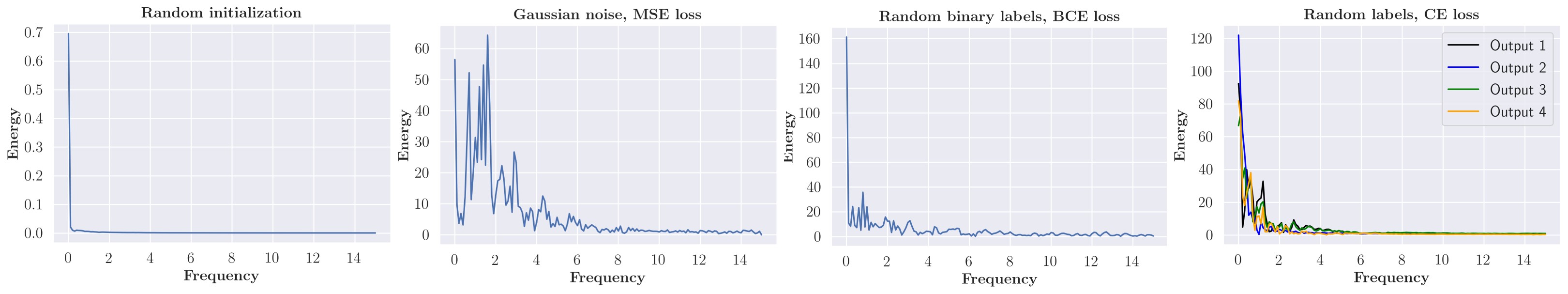
Figure 5: We visualize the spectra of networks after training them with different loss functions and label sampling schemes (the rightmost three plots). All shown methods are able to obtain higher bandwidths than random initialization (leftmost plot). Note that the scale in the $y-$axis is different for each plot. However, in practice, deep classification networks take an infeasible amount of time to converge with MSE loss. Hence, we chose random labels with cross-entropy loss to initialize the deep classification networks with higher bandwidths.

In order to verify that training with random labels indeed induces higher bandwidths on deep classification networks, we visualize the histograms of their first order gradients of the averaged outputs w.r.t. the inputs. It is straightforward to show that (similar to second-order gradients) higher first-order gradients lead to higher bandwidth. For simplicity, consider a function $f:\mathbb{R}\to\mathbb{R}$. Then,

$$f(x)=\int_{\infty}^{\infty}\hat{f}(k)e^{2\pi ikx}dk$$

It follows that,

$$|\frac{df(x)}{dx}| =|2\pi i\int_{\infty}^{\infty}k\hat{f}(k)e^{2\pi ikx}dk|$$ (5)

$$\leq|2\pi|\int_{\infty}^{\infty}|k\hat{f}(k)|dk.$$ (6)

Therefore,

$$\max_{x\in\epsilon}|\frac{df(x)}{dx}|\leq|2\pi|\int_{\infty}^{\infty}|k\hat{f}(k)|dk.$$ (7)

This conclusion can be directly extrapolated to higher-dimensional inputs, where the Fourier transform is also high dimensional. Hence, we feed a batch of images to the networks, and calculate the gradients of the averaged output layer with respect to the input image pixels. Then, we plot the histograms of the gradients (Fig. 6). As illustrated, training with random labels induces higher gradients, and thus, higher bandwidth. Table. 3 compares generalization of deep networks on ImageNet.

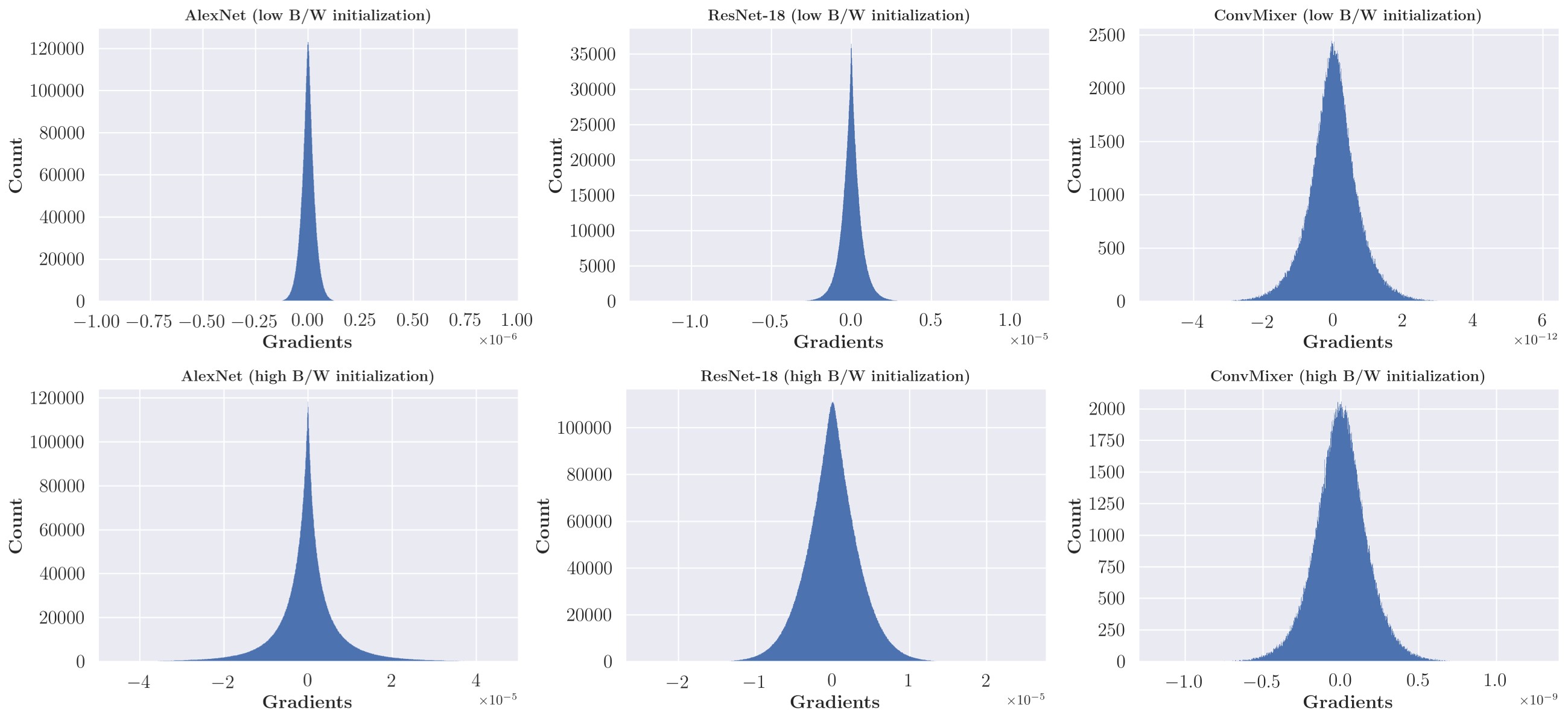
Figure 6: The histograms of the first-order gradients of the outputs with respect to the inputs (a batch of training images) are shown. Low and high bandwidth initializations correspond to Xavier initialization and pre-training with random labels, respectively. Not that the $x-$axis scales are different in each plot. As depicted, training with random labels leads to higher gradients, validating that it indeed leads to higher bandwidths.

ImageNet
Model	Random initialization		High B/W initialization
	Train accuracy	Test accuracy	Train accuracy	Test accuracy
VGG16	$100\%$	$68.19\%$	$100\%$	$55.48$%
ResNet-18	$100\%$	$66.93\%$	$100\%$	$49.17\%$
ConvMixer	$100\%$	$74.19\%$	$100\%$	$45.68\%$

Table 3: Generalization of deep networks in classification over ImageNet. When the models are initialized with higher bandwidths (pre-trained on random labels), the test accuracy drops. We do not use data augmentation in these experiments. We only use three models for this experiment due to the extensive resource usage when training on random labels over ImageNet.

A.3 Convergence-decay rates of frequencies matter for generalization

Earlier, we showed that although all neural networks admit spectral bias, the convergence-decay rates of frequencies change across network types and initialization schemes. Below, we show that these decay rates play an essential role in generalization.

We use a Gaussian network for this experiment. We initialize two instances of the network by 1) using a weight distribution $\mathcal{N}(0,0.03)$, and 2) pre-training the network on a DC signal. In both instances, the network has low bandwidth. Then, we train the network on sparse training data sampled from $3\mathrm{sin}(0.4\pi x)+5\mathrm{sin}(0.2\pi x)$. The results are shown in Fig. 7. Observe that although both networks start from low bandwidth, they exhibit different generalization properties. This is because, having a lower convergence-decay hinders smooth interpolations even in cases where the networks have low initial bandwidth. This is expected, since then, the optimization will begin to affect the higher frequencies before the lower frequencies are converged.

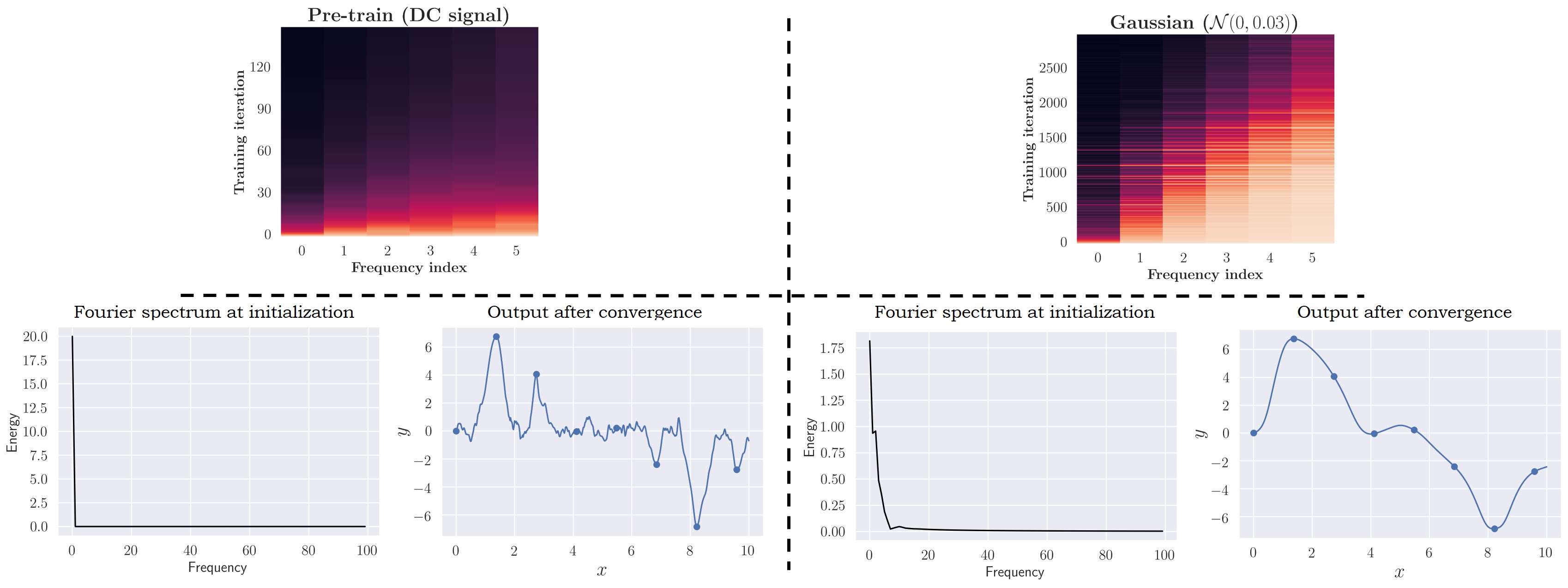
Figure 7: The effect of convergence-decay rate of frequencies on generalization. Left block: We pre-train a Gaussian network on a DC signal to obtain low initial bandwidth. Nevertheless, the network still converges to a non-smooth solution. Right block: The Gaussian network is initialized using a random Gaussian distribution ($\mathcal{N}(0,0.03)$). This method also leads to lower bandwidth. However, in this scenario, the network is able to converge to a smooth solution. At the top, the convergence of frequency components – starting from the corresponding initialization – is shown when training on a signal $g(x)=\sum_{n=1}^{6}\mathrm{sin}(10\pi nx)$. Note that a lower convergence decay rate leads to bad generalization.

To further verify this, we conduct another experiment; see Fig. 8.

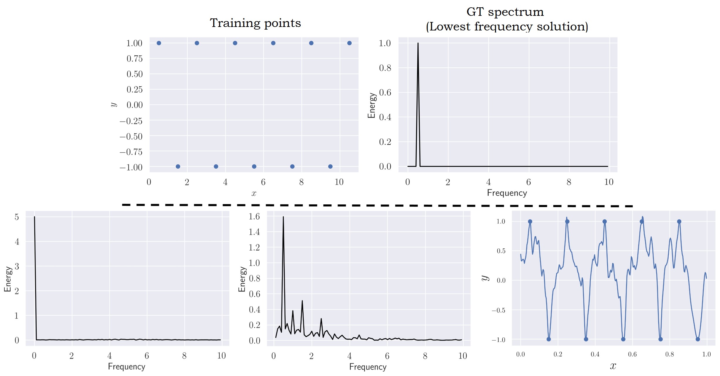
Figure 8: The top block shows sparsely sampled training points from $\mathrm{sin}(\pi x)$ and the corresponding lowest frequency solution that fits the training data. The bottom block shows the spectra of a Gaussian network initialized by pre-training on a DC signal. Even though the network adds a spike at the lowest frequency solution, higher frequencies are also added to the spectrum due to the low convergence-decay rate. This results in a non-smooth interpolation.

A.4 Analyzing the loss landscapes

The flat minima conjecture has been studied since the early work of Hochreiter and Schmidhuber [1994] and Hochreiter and Schmidhuber [1997]. More recently, empirical works showed that the generalization of deep networks is related to the flatness of the minima it is converged to during training [Chaudhari et al., 2019, Keskar et al., 2016]. In order to measure the flatness of loss landscapes, different metrics have been proposed [Tsuzuku et al., 2020, Rangamani et al., 2019, Hochreiter and Schmidhuber, 1994, 1997]. In particular, Chaudhari et al. [2019] and Keskar et al. [2016] showed that minima with low Hessian spectral norm generalize better. In this paper also, we use Hessian-related metrics to measure the flatness. Since the spectral norm alone is not ideal for analyzing the loss landscape of models with a large number of parameters, we also compute the trace and the expected eigenvalue of the Hessian. For computing the Hessian, we use the library provided by Yao et al. [2020]. Fig 9 and Table 4 depict a comparison of loss landscapes in several deep models. Note that our proposed high B/W initialization scheme provides an ideal platform to compare the loss landscapes with different generalization properties.

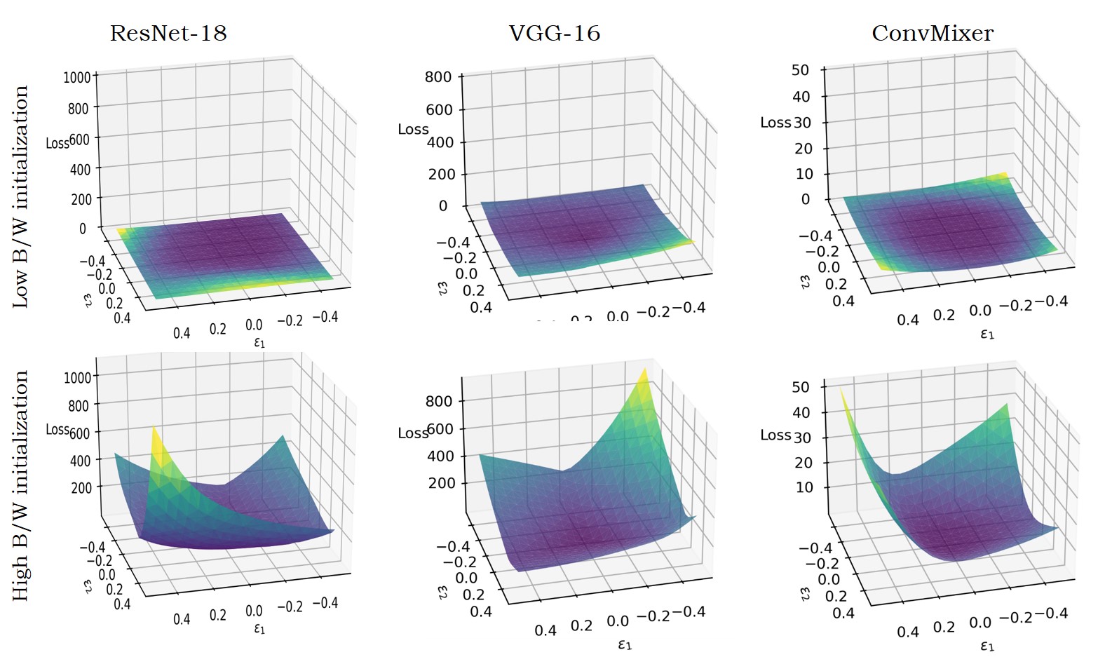
Figure 9: Loss landscapes of deep networks trained on CIFAR10. The proposed high B/W initialization scheme provides an ideal platform to compare the flatness of minima with different generalization properties. Note that ReLU networks exhibit behaviour consistent with the flat minima conjecture.

Model	Hessian-trace	Spectral norm
ResNet-18 (low B/W)	$13560.76$	$2805.47$
ResNet-18 (high B/W)	$28614.19$	$4121.36$
VGG-16 (low B/W)	$10102.51$	$1112.07$
VGG-16 (high B/W)	$14483.90$	$3214.57$
ConvMixer (low B/W)	$0.3242$	$0.028$
ConvMixer (high B/W)	$3.49$	$0.445$

Table 4: Quantitative comparison of the flatness of minima in deep networks. Note that Note that ReLU networks exhibit behaviour consistent with the flat minima conjecture.

References

- Advani et al. [2020] Madhu S Advani, Andrew M Saxe, and Haim Sompolinsky. High-dimensional dynamics of generalization error in neural networks. Neural Networks, 132:428–446, 2020.
- Ali et al. [2020] Alnur Ali, Edgar Dobriban, and Ryan Tibshirani. The implicit regularization of stochastic gradient flow for least squares. In International conference on machine learning, pages 233–244. PMLR, 2020.
- Arora et al. [2019] Sanjeev Arora, Nadav Cohen, Wei Hu, and Yuping Luo. Implicit regularization in deep matrix factorization. Advances in Neural Information Processing Systems, 32, 2019.
- Basher et al. [2021] Abol Basher, Muhammad Sarmad, and Jani Boutellier. Lightsal: Lightweight sign agnostic learning for implicit surface representation. arXiv preprint arXiv:2103.14273, 2021.
- Brutzkus and Globerson [2020] Alon Brutzkus and Amir Globerson. On the inductive bias of a cnn for orthogonal patterns distributions. arXiv e-prints, pages arXiv–2002, 2020.
- Chaudhari et al. [2019] Pratik Chaudhari, Anna Choromanska, Stefano Soatto, Yann LeCun, Carlo Baldassi, Christian Borgs, Jennifer Chayes, Levent Sagun, and Riccardo Zecchina. Entropy-sgd: Biasing gradient descent into wide valleys. Journal of Statistical Mechanics: Theory and Experiment, 2019(12):124018, 2019.
- Chen and Zhang [2019] Zhiqin Chen and Hao Zhang. Learning implicit fields for generative shape modeling. In Proceedings of the IEEE/CVF Conference on Computer Vision and Pattern Recognition, pages 5939–5948, 2019.
- Chizat and Bach [2020] Lenaic Chizat and Francis Bach. Implicit bias of gradient descent for wide two-layer neural networks trained with the logistic loss. In Conference on Learning Theory, pages 1305–1338. PMLR, 2020.
- Chizat et al. [2019] Lenaic Chizat, Edouard Oyallon, and Francis Bach. On lazy training in differentiable programming. Advances in Neural Information Processing Systems, 32, 2019.
- Craven and Wahba [1978] Peter Craven and Grace Wahba. Smoothing noisy data with spline functions. Numerische mathematik, 31(4):377–403, 1978.
- Deng et al. [2020] Boyang Deng, John P Lewis, Timothy Jeruzalski, Gerard Pons-Moll, Geoffrey Hinton, Mohammad Norouzi, and Andrea Tagliasacchi. Nasa neural articulated shape approximation. In Computer Vision–ECCV 2020: 16th European Conference, Glasgow, UK, August 23–28, 2020, Proceedings, Part VII 16, pages 612–628. Springer, 2020.
- Dinh [2017] Laurent and Pascanu, Razvan and Bengio, Samy and Bengio, Yoshua Dinh. Sharp Minima Can Generalize for Deep Nets. ICML, 2017.
- Genova et al. [2020] Kyle Genova, Forrester Cole, Avneesh Sud, Aaron Sarna, and Thomas Funkhouser. Local deep implicit functions for 3d shape. In Proceedings of the IEEE/CVF Conference on Computer Vision and Pattern Recognition, pages 4857–4866, 2020.
- Gidel et al. [2019] Gauthier Gidel, Francis Bach, and Simon Lacoste-Julien. Implicit regularization of discrete gradient dynamics in linear neural networks. arXiv preprint arXiv:1904.13262, 2019.
- Glorot and Bengio [2010] Xavier Glorot and Yoshua Bengio. Understanding the difficulty of training deep feedforward neural networks. In Proceedings of the thirteenth international conference on artificial intelligence and statistics, pages 249–256. JMLR Workshop and Conference Proceedings, 2010.
- Goldt et al. [2019] Sebastian Goldt, Madhu Advani, Andrew M Saxe, Florent Krzakala, and Lenka Zdeborová. Dynamics of stochastic gradient descent for two-layer neural networks in the teacher-student setup. Advances in neural information processing systems, 32, 2019.
- Grafakos [2008] L. Grafakos. Classical Fourier Analysis. Number 249 in Graduate Texts in Mathematics. Springer, Second Edition edition, 2008.
- Gunasekar et al. [2017] Suriya Gunasekar, Blake E Woodworth, Srinadh Bhojanapalli, Behnam Neyshabur, and Nati Srebro. Implicit regularization in matrix factorization. Advances in Neural Information Processing Systems, 30, 2017.
- Gunasekar et al. [2018] Suriya Gunasekar, Jason Lee, Daniel Soudry, and Nathan Srebro. Characterizing implicit bias in terms of optimization geometry. In International Conference on Machine Learning, pages 1832–1841. PMLR, 2018.
- He et al. [2020] Fengxiang He, Tongliang Liu, and Dacheng Tao. Why resnet works? residuals generalize. IEEE transactions on neural networks and learning systems, 31(12):5349–5362, 2020.
- He et al. [2016] Kaiming He, Xiangyu Zhang, Shaoqing Ren, and Jian Sun. Deep residual learning for image recognition. In Proceedings of the IEEE conference on computer vision and pattern recognition, pages 770–778, 2016.
- Heiss et al. [2019] Jakob Heiss, Josef Teichmann, and Hanna Wutte. How implicit regularization of neural networks affects the learned function–part i. arXiv, pages 1911–02903, 2019.
- Henzler et al. [2020] Philipp Henzler, Niloy J Mitra, and Tobias Ritschel. Learning a neural 3d texture space from 2d exemplars. In Proceedings of the IEEE/CVF Conference on Computer Vision and Pattern Recognition, pages 8356–8364, 2020.
- Hochreiter and Schmidhuber [1994] Sepp Hochreiter and Jürgen Schmidhuber. Simplifying neural nets by discovering flat minima. Advances in neural information processing systems, 7, 1994.
- Hochreiter and Schmidhuber [1997] Sepp Hochreiter and Jürgen Schmidhuber. Flat minima. Neural computation, 9(1):1–42, 1997.
- Hu et al. [2018] Jie Hu, Li Shen, and Gang Sun. Squeeze-and-excitation networks. In Proceedings of the IEEE conference on computer vision and pattern recognition, pages 7132–7141, 2018.
- Huang et al. [2017] Gao Huang, Zhuang Liu, Laurens Van Der Maaten, and Kilian Q Weinberger. Densely connected convolutional networks. In Proceedings of the IEEE conference on computer vision and pattern recognition, pages 4700–4708, 2017.
- Huang et al. [2020] Kaixuan Huang, Yuqing Wang, Molei Tao, and Tuo Zhao. Why do deep residual networks generalize better than deep feedforward networks?—a neural tangent kernel perspective. Advances in neural information processing systems, 33:2698–2709, 2020.
- Jacot et al. [2018a] A. Jacot, F. Gabriel, and C. Hongler. Neural Tangent Kernel: Convergence and Generalization in Neural Networks. NeurIPS, 2018a.
- Jacot et al. [2018b] Arthur Jacot, Franck Gabriel, and Clément Hongler. Neural tangent kernel: Convergence and generalization in neural networks. arXiv preprint arXiv:1806.07572, 2018b.
- Jastrzębski et al. [2017] Stanisław Jastrzębski, Zachary Kenton, Devansh Arpit, Nicolas Ballas, Asja Fischer, Yoshua Bengio, and Amos Storkey. Three factors influencing minima in sgd. arXiv preprint arXiv:1711.04623, 2017.
- Ji and Telgarsky [2018] Ziwei Ji and Matus Telgarsky. Gradient descent aligns the layers of deep linear networks. arXiv preprint arXiv:1810.02032, 2018.
- Ji and Telgarsky [2019] Ziwei Ji and Matus Telgarsky. The implicit bias of gradient descent on nonseparable data. In Conference on Learning Theory, pages 1772–1798. PMLR, 2019.
- Keskar et al. [2016] Nitish Shirish Keskar, Dheevatsa Mudigere, Jorge Nocedal, Mikhail Smelyanskiy, and Ping Tak Peter Tang. On large-batch training for deep learning: Generalization gap and sharp minima. arXiv preprint arXiv:1609.04836, 2016.
- Kimeldorf and Wahba [1970] George S Kimeldorf and Grace Wahba. A correspondence between bayesian estimation on stochastic processes and smoothing by splines. The Annals of Mathematical Statistics, 41(2):495–502, 1970.
- Krizhevsky [2014] Alex Krizhevsky. One weird trick for parallelizing convolutional neural networks. arXiv preprint arXiv:1404.5997, 2014.
- Lampinen and Ganguli [2018] Andrew K Lampinen and Surya Ganguli. An analytic theory of generalization dynamics and transfer learning in deep linear networks. arXiv preprint arXiv:1809.10374, 2018.
- Li et al. [2018] Yuanzhi Li, Tengyu Ma, and Hongyang Zhang. Algorithmic regularization in over-parameterized matrix sensing and neural networks with quadratic activations. In Conference On Learning Theory, pages 2–47. PMLR, 2018.
- Luo et al. [2019] Tao Luo, Zheng Ma, Zhi-Qin John Xu, and Yaoyu Zhang. Theory of the frequency principle for general deep neural networks. arXiv preprint arXiv:1906.09235, 2019.
- Luo et al. [2020] Tao Luo, Zheng Ma, Zhi-Qin John Xu, and Yaoyu Zhang. On the exact computation of linear frequency principle dynamics and its generalization. arXiv preprint arXiv:2010.08153, 2020.
- Ma et al. [2018] Cong Ma, Kaizheng Wang, Yuejie Chi, and Yuxin Chen. Implicit regularization in nonconvex statistical estimation: Gradient descent converges linearly for phase retrieval and matrix completion. In International Conference on Machine Learning, pages 3345–3354. PMLR, 2018.
- Martin-Brualla et al. [2021] Ricardo Martin-Brualla, Noha Radwan, Mehdi SM Sajjadi, Jonathan T Barron, Alexey Dosovitskiy, and Daniel Duckworth. Nerf in the wild: Neural radiance fields for unconstrained photo collections. In Proceedings of the IEEE/CVF Conference on Computer Vision and Pattern Recognition, pages 7210–7219, 2021.
- Mei et al. [2019] Song Mei, Theodor Misiakiewicz, and Andrea Montanari. Mean-field theory of two-layers neural networks: dimension-free bounds and kernel limit. In Conference on Learning Theory, pages 2388–2464. PMLR, 2019.
- Mildenhall et al. [2020] Ben Mildenhall, Pratul P Srinivasan, Matthew Tancik, Jonathan T Barron, Ravi Ramamoorthi, and Ren Ng. Nerf: Representing scenes as neural radiance fields for view synthesis. In European Conference on Computer Vision, pages 405–421. Springer, 2020.
- Min et al. [2021] Hancheng Min, Salma Tarmoun, René Vidal, and Enrique Mallada. On the explicit role of initialization on the convergence and implicit bias of overparametrized linear networks. In International Conference on Machine Learning, pages 7760–7768. PMLR, 2021.
- Moroshko et al. [2020] Edward Moroshko, Blake E Woodworth, Suriya Gunasekar, Jason D Lee, Nati Srebro, and Daniel Soudry. Implicit bias in deep linear classification: Initialization scale vs training accuracy. Advances in neural information processing systems, 33:22182–22193, 2020.
- Mu et al. [2021] Jiteng Mu, Weichao Qiu, Adam Kortylewski, Alan Yuille, Nuno Vasconcelos, and Xiaolong Wang. A-sdf: Learning disentangled signed distance functions for articulated shape representation. arXiv preprint arXiv:2104.07645, 2021.
- Mulayoff and Michaeli [2020] Rotem Mulayoff and Tomer Michaeli. Unique properties of flat minima in deep networks. In International Conference on Machine Learning, pages 7108–7118. PMLR, 2020.
- Niemeyer et al. [2020] Michael Niemeyer, Lars Mescheder, Michael Oechsle, and Andreas Geiger. Differentiable volumetric rendering: Learning implicit 3d representations without 3d supervision. In Proceedings of the IEEE/CVF Conference on Computer Vision and Pattern Recognition, pages 3504–3515, 2020.
- Oechsle et al. [2019] Michael Oechsle, Lars Mescheder, Michael Niemeyer, Thilo Strauss, and Andreas Geiger. Texture fields: Learning texture representations in function space. In Proceedings of the IEEE/CVF International Conference on Computer Vision, pages 4531–4540, 2019.
- Oymak and Soltanolkotabi [2019] Samet Oymak and Mahdi Soltanolkotabi. Overparameterized nonlinear learning: Gradient descent takes the shortest path? In International Conference on Machine Learning, pages 4951–4960. PMLR, 2019.
- Park et al. [2019] Jeong Joon Park, Peter Florence, Julian Straub, Richard Newcombe, and Steven Lovegrove. Deepsdf: Learning continuous signed distance functions for shape representation. In Proceedings of the IEEE/CVF Conference on Computer Vision and Pattern Recognition, pages 165–174, 2019.
- Park et al. [2021] Keunhong Park, Utkarsh Sinha, Jonathan T Barron, Sofien Bouaziz, Dan B Goldman, Steven M Seitz, and Ricardo Martin-Brualla. Nerfies: Deformable neural radiance fields. In Proceedings of the IEEE/CVF International Conference on Computer Vision, pages 5865–5874, 2021.
- Pumarola et al. [2021] Albert Pumarola, Enric Corona, Gerard Pons-Moll, and Francesc Moreno-Noguer. D-nerf: Neural radiance fields for dynamic scenes. In Proceedings of the IEEE/CVF Conference on Computer Vision and Pattern Recognition, pages 10318–10327, 2021.
- Rahaman et al. [2019] Nasim Rahaman, Aristide Baratin, Devansh Arpit, Felix Draxler, Min Lin, Fred Hamprecht, Yoshua Bengio, and Aaron Courville. On the spectral bias of neural networks. In International Conference on Machine Learning, pages 5301–5310. PMLR, 2019.
- Ramasinghe and Lucey [2021] Sameera Ramasinghe and Simon Lucey. Beyond periodicity: Towards a unifying framework for activations in coordinate-mlps. arXiv preprint arXiv:2111.15135, 2021.
- Rangamani et al. [2019] Akshay Rangamani, Nam H Nguyen, Abhishek Kumar, Dzung Phan, Sang H Chin, and Trac D Tran. A scale invariant flatness measure for deep network minima. arXiv preprint arXiv:1902.02434, 2019.
- Razin et al. [2021] Noam Razin, Asaf Maman, and Nadav Cohen. Implicit regularization in tensor factorization. In International Conference on Machine Learning, pages 8913–8924. PMLR, 2021.
- Rebain et al. [2021] Daniel Rebain, Wei Jiang, Soroosh Yazdani, Ke Li, Kwang Moo Yi, and Andrea Tagliasacchi. Derf: Decomposed radiance fields. In Proceedings of the IEEE/CVF Conference on Computer Vision and Pattern Recognition, pages 14153–14161, 2021.
- Reinsch [1967] Christian H Reinsch. Smoothing by spline functions. Numerische mathematik, 10(3):177–183, 1967.
- Saito et al. [2019] Shunsuke Saito, Zeng Huang, Ryota Natsume, Shigeo Morishima, Angjoo Kanazawa, and Hao Li. Pifu: Pixel-aligned implicit function for high-resolution clothed human digitization. In Proceedings of the IEEE/CVF International Conference on Computer Vision, pages 2304–2314, 2019.
- Simonyan and Zisserman [2014] Karen Simonyan and Andrew Zisserman. Very deep convolutional networks for large-scale image recognition. arXiv preprint arXiv:1409.1556, 2014.
- Simsekli et al. [2019] Umut Simsekli, Levent Sagun, and Mert Gurbuzbalaban. A tail-index analysis of stochastic gradient noise in deep neural networks. In International Conference on Machine Learning, pages 5827–5837. PMLR, 2019.
- Sitzmann et al. [2019] Vincent Sitzmann, Michael Zollhöfer, and Gordon Wetzstein. Scene representation networks: Continuous 3d-structure-aware neural scene representations. arXiv preprint arXiv:1906.01618, 2019.
- Sitzmann et al. [2020] Vincent Sitzmann, Julien Martel, Alexander Bergman, David Lindell, and Gordon Wetzstein. Implicit neural representations with periodic activation functions. Advances in Neural Information Processing Systems, 33, 2020.
- Soudry et al. [2018] Daniel Soudry, Elad Hoffer, Mor Shpigel Nacson, Suriya Gunasekar, and Nathan Srebro. The implicit bias of gradient descent on separable data. The Journal of Machine Learning Research, 19(1):2822–2878, 2018.
- Tan and Le [2019] Mingxing Tan and Quoc Le. Efficientnet: Rethinking model scaling for convolutional neural networks. In International conference on machine learning, pages 6105–6114. PMLR, 2019.
- Tancik et al. [2020] Matthew Tancik, Pratul P Srinivasan, Ben Mildenhall, Sara Fridovich-Keil, Nithin Raghavan, Utkarsh Singhal, Ravi Ramamoorthi, Jonathan T Barron, and Ren Ng. Fourier features let networks learn high frequency functions in low dimensional domains. arXiv preprint arXiv:2006.10739, 2020.
- Tiwari et al. [2021] Garvita Tiwari, Nikolaos Sarafianos, Tony Tung, and Gerard Pons-Moll. Neural-gif: Neural generalized implicit functions for animating people in clothing. In Proceedings of the IEEE/CVF International Conference on Computer Vision, pages 11708–11718, 2021.
- Trockman and Kolter [2022] Asher Trockman and J Zico Kolter. Patches are all you need? arXiv preprint arXiv:2201.09792, 2022.
- Tsuzuku et al. [2020] Yusuke Tsuzuku, Issei Sato, and Masashi Sugiyama. Normalized flat minima: Exploring scale invariant definition of flat minima for neural networks using pac-bayesian analysis. In International Conference on Machine Learning, pages 9636–9647. PMLR, 2020.
- Wang et al. [2021] Zirui Wang, Shangzhe Wu, Weidi Xie, Min Chen, and Victor Adrian Prisacariu. Nerf–: Neural radiance fields without known camera parameters. arXiv preprint arXiv:2102.07064, 2021.
- Wei et al. [2019] Colin Wei, Jason D Lee, Qiang Liu, and Tengyu Ma. Regularization matters: Generalization and optimization of neural nets vs their induced kernel. Advances in Neural Information Processing Systems, 32, 2019.
- Wu et al. [2018] Lei Wu, Chao Ma, et al. How sgd selects the global minima in over-parameterized learning: A dynamical stability perspective. Advances in Neural Information Processing Systems, 31, 2018.
- Wu et al. [2019] Xiaoxia Wu, Edgar Dobriban, Tongzheng Ren, Shanshan Wu, Zhiyuan Li, Suriya Gunasekar, Rachel Ward, and Qiang Liu. Implicit regularization of normalization methods. arXiv preprint arXiv:1911.07956, 2019.
- Xiang et al. [2021] Fanbo Xiang, Zexiang Xu, Milos Hasan, Yannick Hold-Geoffroy, Kalyan Sunkavalli, and Hao Su. Neutex: Neural texture mapping for volumetric neural rendering. In Proceedings of the IEEE/CVF Conference on Computer Vision and Pattern Recognition, pages 7119–7128, 2021.
- Xu et al. [2019] Zhi-Qin John Xu, Yaoyu Zhang, and Yanyang Xiao. Training behavior of deep neural network in frequency domain. In International Conference on Neural Information Processing, pages 264–274. Springer, 2019.
- Xu [2018] Zhiqin John Xu. Understanding training and generalization in deep learning by fourier analysis. arXiv preprint arXiv:1808.04295, 2018.
- Yao et al. [2020] Zhewei Yao, Amir Gholami, Kurt Keutzer, and Michael W Mahoney. Pyhessian: Neural networks through the lens of the hessian. In 2020 IEEE international conference on big data (Big data), pages 581–590. IEEE, 2020.
- Yu et al. [2021] Alex Yu, Vickie Ye, Matthew Tancik, and Angjoo Kanazawa. pixelnerf: Neural radiance fields from one or few images. In Proceedings of the IEEE/CVF Conference on Computer Vision and Pattern Recognition, pages 4578–4587, 2021.
- Yun et al. [2020] Chulhee Yun, Shankar Krishnan, and Hossein Mobahi. A unifying view on implicit bias in training linear neural networks. arXiv preprint arXiv:2010.02501, 2020.
- Zhang et al. [2016] Chiyuan Zhang, Samy Bengio, Moritz Hardt, Benjamin Recht, and Oriol Vinyals. Understanding deep learning requires rethinking generalization. arXiv e-prints, pages arXiv–1611, 2016.
- Zhang et al. [2019] Yaoyu Zhang, Zhi-Qin John Xu, Tao Luo, and Zheng Ma. Explicitizing an implicit bias of the frequency principle in two-layer neural networks. arXiv preprint arXiv:1905.10264, 2019.
- Zheng et al. [2021] Jianqiao Zheng, Sameera Ramasinghe, and Simon Lucey. Rethinking positional encoding. arXiv preprint arXiv:2107.02561, 2021.