Low-latency Mini-batch GNN Inference on
CPU-FPGA Heterogeneous Platform

Abstract.

Mini-batch inference of Graph Neural Networks (GNNs) is a key problem in many real-world applications. Recently, a GNN design principle of model depth-receptive field decoupling has been proposed to address the well-known issue of neighborhood explosion. Decoupled GNN models achieve higher accuracy than original models and demonstrate excellent scalability for mini-batch inference.

We map Decoupled GNNs onto CPU-FPGA heterogeneous platforms to achieve low-latency mini-batch inference. On the FPGA platform, we design a novel GNN hardware accelerator with an adaptive datapath denoted Adaptive Computation Kernel (ACK) that can execute various computation kernels of GNNs with low-latency: (1) for dense computation kernels expressed as matrix multiplication, ACK works as a systolic array with fully localized connections, (2) for sparse computation kernels, ACK follows the scatter-gather paradigm and works as multiple parallel pipelines to support the irregular connectivity of graphs. The proposed task scheduling hides the CPU-FPGA data communication overhead to reduce the inference latency. We develop a fast design space exploration algorithm to generate a single accelerator for multiple target GNN models. We implement our accelerator on a state-of-the-art CPU-FPGA platform and evaluate the performance using three representative models (GCN, GraphSAGE, and GAT). Results show that our CPU-FPGA implementation achieves $21.4-50.8\times$, $2.9-21.6\times$, $4.7\times$ latency reduction compared with state-of-the-art implementations on CPU-only, CPU-GPU and CPU-FPGA platforms.

1. Introduction

Graph Neural Networks (GNNs) have become a revolutionary technique in graph-based machine learning. GNNs outperform traditional algorithms in various applications (Hu et al., 2020). Recently, many vendors have adopted GNNs in their commercial systems, such as recommendation systems (Yang, 2019), social media (Lerer et al., 2019), knowledge databases (Mernyei and Cangea, 2020), etc. In these systems, data are represented as graphs, where vertices correspond to entities and edges encode the relationship among entities. A fundamental task is mini-batch GNN inference: given a set of target vertices, infer the embeddings (vector representation) of the vertices with low-latency.

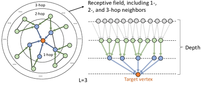
Figure 1. Recursive message passing of GNNs results in exponential computation and communication cost, and low computation-to-communication (C2C) ratio

There are two major challenges for mini-batch inference. (1) neighborhood explosion: the widely used GNNs, such as GCN (Kipf and Welling, 2016), GraphSAGE (Hamilton et al., 2017), GIN (Xu et al., 2018), GAT (Veličković et al., 2017), follow the message-passing paradigm that in a $L$-layer model, a vertex recursively aggregates information from its $L$-hop neighbors. The receptive field is defined as the set of neighbors passing messages to the target vertex. In the above example (Figure 1), the receptive field consists of all the vertices within $L$-hop. In a large graph, the size of the receptive field quickly explodes w.r.t. model depth $L$. Therefore, mini-batch GNN inference suffers from two issues. First, the computation and communication costs grow exponentially with the depth of GNN. This hinders the deployment of deeper GNNs on memory constrained accelerators. It has been proven (Gallicchio and Micheli, 2020; Li et al., 2021; Zeng et al., 2021) that deeper GNNs have higher accuracy than shallower ones. Second, the computation-to-communication (C2C) ratio is low, thus making it not suitable for hardware acceleration. (2) load imbalance: GNN computation involves various kinds of kernels, including dense computation kernels and sparse computation kernels. To support various kernels, previous work (Yan et al., 2020; Zeng and Prasanna, 2020; Zhang et al., 2021) designed hybrid accelerators that for each kernel, a dedicated hardware module is designed and initialized independently. For example, in GraphACT (Zeng and Prasanna, 2020), the Feature Aggregation Module executes the sparse kernel and Feature Transformation Module executes the dense kernel. However, it is challenging to achieve load balance among hardware modules in a hybrid accelerator. For example, the workload of feature aggregation is unpredictable and depends on the connectivity of the input graphs. The load imbalance leads to hardware under-utilization and extra latency.

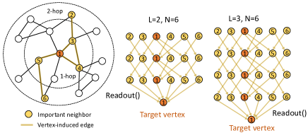
Figure 2. An example of Decoupled GNN model

Recently, model depth-receptive field decoupling (Zeng et al., 2021) is proposed to resolve the neighborhood explosion challenge. Under the decoupling principle, GNN depth is independent of receptive field. As shown in Figure 2, for a target vertex, it selects a small number of important neighbors as the receptive field $\mathcal{N}$, and then applies an arbitrary deep GNN upon such pre-defined $\mathcal{N}$. The key property of a Decoupled GNN is that the size of $\mathcal{N}$ remains fixed while the GNN becomes deeper, thus reducing the computation complexity from exponential to linear w.r.t. model depth. Each layer only propagate information within $\mathcal{N}$. Compared with original GNN models (Figure 1), the Decoupled GNN models theoretically lead to significantly less computation cost and memory bandwidth requirement and thus are well-suited for hardware acceleration.

While there have been many GNN accelerators (Yan et al., 2020; Geng et al., 2020; Zhang et al., 2021; Liang et al., 2020; Zeng and Prasanna, 2020; Lin et al., 2021) proposed, none of them is designed or optimized for low-latency mini-batch inference. Specifically, (Yan et al., 2020; Geng et al., 2020; Zhang et al., 2021; Liang et al., 2020) are for full-graph inference and (Zeng and Prasanna, 2020) is for mini-batch training. Full-graph GNN inference has very different computation characteristics from mini-batch inference. In full-graph inference, all vertices in the graph are target vertices. Through careful vertex reordering (Zhang et al., 2020; Geng et al., 2021) and graph partitioning (Yan et al., 2020; Zhang et al., 2021), full-graph execution can achieve high data reuse by exploiting common neighbors. However, in mini-batch inference, it is more challenging to improve data reuse since the target vertices rarely share common neighbors. In addition, GraphACT (Zeng and Prasanna, 2020) is built on specific training algorithm (Zeng et al., 2020) to improve computation-to-communication ratio only during training. While the computation pipeline of GraphACT can be adapted to inference, its performance may be sub-optimal due to load imbalance (challenge (2) above).

In this paper, we map the inference process of Decoupled models on CPU-FPGA platforms for low-latency mini-batch inference. To this end, we design a unified hardware accelerator consisting of (1) adaptive datapath that can execute various computation kernels of GNNs with low-latency, thus overcoming the load-imbalance challenge, (2) memory organization that can hide data communication overhead to further reduce the inference latency. Our main contributions are:

• By analyzing the computation and communication cost of mini-batch GNN inference, we identify “model depth-receptive field” decoupling as a key model design technique towards low-latency accelerator design.

• We propose a system design on CPU-FPGA platforms to achieve low-latency mini-batch inference:

  • We develop a novel hardware accelerator with two execution modes that can execute various GNN computation kernels (e.g., feature aggregation, feature transformation, attention) with low-latency.

  • We customize the memory organization to achieve low-latency data communication, and proposed double/triple buffering techniques to hide communication overhead.

  • We perform task scheduling to hide the CPU-FPGA data movement overhead.

• We develop a design space exploration algorithm that given 1) specification of the target FPGA device, and 2) a set of target GNN models with various depths and receptive field sizes, it generates a single hardware that achieves low-latency inference without reconfiguration.

• We implement our hardware accelerator on a state-of-the-art CPU-FPGA platform and evaluate the performance using three representative models (GCN, GraphSAGE, GAT). Experiments show that our CPU-FPGA implementation achieves $21.4-50.8\times$, $2.9-21.6\times$, $4.7\times$ speedup compared with state-of-the-art implementations on CPU-only, CPU-GPU and CPU-FPGA platforms.

2. background

2.1. Field Programmable Gate Array

Recently, Field Programmable Gate Array (FPGA) has been extensively studied for accelerating machine learning tasks (Geng et al., 2020; Zhang et al., 2021; Zeng and Prasanna, 2020). A FPGA device deployed in a cloud has significant hardware resources, including Lookup Tables (LUTs), Digital Signal Processing units (DSPs), on-chip memories (BRAMs, URAMs) and programmable interconnections. Programmability of FPGA allows users to exploit the fine-grained data parallelism in a computation task. An FPGA is more attractive for low-latency computation compared with GPU which has coarse-grained thread-level parallelism.

GNN acceleration on FPGA: As discussed in Section 1, previous GNN accelerators on FPGA such as GraphACT (Zeng and Prasanna, 2020), BoostGCN (Zhang et al., 2021), Deepburning-GL (Liang et al., 2020) , AWB-GCN (Lin et al., 2021), are not suitable for mini-batch GNN inference. In this work, we develop an optimized FPGA accelerator to achieve low-latency mini-batch GNN inference (Section 3).

Table 1. Notations

Notation Description Notation Description $\mathcal{G}(\mathcal{V},\mathcal{E})$ input graph $v_{i}$ $i^{\text{th}}$ vertex $\mathcal{V}$ set of vertices $e_{ij}$ edge from $v_{i}$ to $v_{j}$ $\mathcal{E}$ set of edges $L$ number of GNN layers $N$ # of vertices in the receptive field $\mathcal{N}_{L}(i)$ $L$-hop neighbors of $v_{i}$ $\bm{h}_{i}^{l}$ feature vector of $v_{i}$ at layer $l$ $\mathcal{N}$ receptive field $\bm{H}$ vertex feature matrix $\bm{W}^{l}$ weight matrix of layer $l$

2.2. Graph Neural Network

The related notations are defined in Table 1. Graph Neural Networks (GNNs) (Kipf and Welling, 2016; Hamilton et al., 2017) are proposed for representation learning on graphs. GNNs operate on the graph $\mathcal{G}(\mathcal{V},\mathcal{E})$ and follow the message-passing paradigm that vertices recursively aggregate information from the neighbors. As shown in Algorithm 1, $\bm{h}^{L}_{v}$ denotes the last-layer embedding of the target vertex $v$. The GNN output $\bm{h}^{L}_{v}$ can be used for many downstream tasks, such as node classification (Hamilton et al., 2017; Kipf and Welling, 2016), link prediction (Zhang and Chen, 2018), graph classification (Ying et al., 2018), etc.

Algorithm 1 Recursive message-passing paradigm of GNN

1:Input graph: $\mathcal{G}(\mathcal{V},\mathcal{E})$; Initial vertex features of input graph: $\left\{\bm{h}^{0}_{1},\bm{h}^{0}_{2},\bm{h}^{0}_{3},...,\bm{h}^{0}_{|\mathcal{V}|}\right\}$; Set of target vertices: $\{v_{1},v_{2},...,v_{m}\}$

2:Output embeddings: $\left\{\bm{h}^{L}_{v_{1}},\bm{h}^{L}_{v_{2}},\bm{h}^{L}_{v_{3}},...,\bm{h}^{L}_{v_{m}}\right\}$

3:for $v_{i}\in\{v_{1},v_{2},...,v_{m}\}$ do

4:    for $l=1$ to $L$  do

5:         for $v_{j}\in\mathcal{N}_{L-l}(i)$  do

6:             $\bm{z}_{j}^{l}=\text{aggregate}\left(\bm{h}_{k}^{l-1}:k\in\mathcal{N}_{1}(j)\bigcap\mathcal{N}_{L-l+1}(i)\right)$

7:             $\bm{h}_{j}^{l}=\text{update}\left(\bm{z}_{j}^{l},\bm{h}_{j}^{l-1},\bm{W}^{l}\right)$              

In an $L$-layer model, a target vertex $v$ aggregates information from the neighbors within $L$-hop. The neighbors within $L$-hop form the receptive field of $v$. The number of vertices $N$ in the receptive field grows exponentially with the depth $L$ of the model: $N\approx\mathcal{O}(d^{L})$, where $d$ is the average degree of the graph. We denote GNNs following such recursive message-passing paradigm as Coupled models since the size of receptive field $N$ depends on the model depth $L$. The GNN model weights includes the weight matrix $\bm{W}^{l}(1\leqslant l\leqslant L)$ of each layer and the size of weight matrices are independent of graph size.

Specification of a Coupled model: A Coupled GNN model is specified by: (1) number of layers $L$, (2) $\text{aggregate}()$ function that defines operator for aggregating the neighbor information (e.g., $\text{aggregate}()$ of GCN (Kipf and Welling, 2016): $\bm{z}_{j}^{l}=\text{Sum}\big{(}\frac{1}{\sqrt{D(j)\cdot D(i)}}\cdot\bm{h}_{i}^{l-1}:v_{i}\in\mathcal{N}_{1}(j)\cup\{j\}\big{)}$), (3) hidden dimension of each layer $f_{l}$ for $0\leqslant l\leqslant L$, (4) $\text{update}()$ function (e.g., $\bm{h}_{j}^{l}=ReLU(\bm{W}^{l}\bm{h}_{j}^{l-1})$) with weight matrix $\bm{W}^{l}\leavevmode\nobreak\ (1\leqslant l\leqslant L)$.

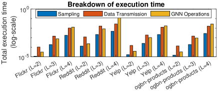
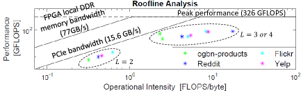
Figure 3. Experimental analysis of mini-batch inference using Coupled GraphSAGE (Kipf and Welling, 2016) model: (1) Breakdown of execution time, (2) Roofline analysis (vertical axis is in log-scale)

To understand the low C2C ratio of Coupled GNNs, we profile the execution of mini-batch inference of GraphSAGE (Hamilton et al., 2017) using a prior FPGA accelerator (GraphACT) (Zeng and Prasanna, 2020) using the CPU-FPGA platform (Baseline 3) described in Section 5.1. The graph is stored in the external memory of the host processor, since the sizes of realistic graphs are often much larger than the on-chip capacity of GPUs and FPGAs. We further perform vertex sampling on the $L$-hop neighborhood (following the recommended parameters (Hamilton et al., 2017)) to optimize performance. See descriptions of the four datasets in Section 4. As shown in Figure 3-(1), the data transmission between CPU and FPGA incurs significant execution time overhead because the number of neighbors grows exponentially with the depth of GNN model. The execution time also increases exponentially with the GNN depth. The roofline analysis (Figure 3) demonstrates that mini-batch inference of Coupled GNN model is memory-bound, and the overall performance is limited by the available PCIe bandwidth. Moreover, the hardware accelerator has low utilization $<30\%$ (computed by $\frac{\text{achieved performance}}{\text{peak performance}}\times 100\%$).

2.3. Model Depth-receptive Field Decoupling

Algorithm 2 Inference process of Decoupled GNN models

1:$\mathcal{G}(\mathcal{V},\mathcal{E},\bm{X}^{0})$; Number of layers $L$; Size of receptive field $N$; A batch of target vertices $\mathcal{V}_{t}$; GNN layer operators (aggregate(), update());

2:Node embeddings of target vertices: $\{h_{v}^{L}:v\in\mathcal{V}_{t}\}$

3:for $v\in\mathcal{V}_{t}$  do

4:    Identify $N$ important neighbors $\mathcal{N}_{imp}(v)$ for $v$.

5:    Build the vertex-induced subgraph $\mathcal{G}^{\prime}(v)$ using $\mathcal{N}_{imp}(v)\bigcup\{v\}$

6:    Extract the input vertex features $\mathcal{F}(v)=\{h_{u}^{0}:u\in\mathcal{G}^{\prime}(v)\}$.

7:    for $l\leftarrow 1$ to $L$  do

8:         Message passing within $\mathcal{G}^{\prime}(v)$ using the layer-$l$ operators     

9:    Obtain the node embedding of vertex $v$ through $\text{Readout}()$.

Recently, (Zeng et al., 2021) proposed a decoupling principle where the GNN depth $L$ and the receptive field size $N$ are specified independently. Decoupling is proposed based on the observation that in the Coupled GNN models, most neighbors involved in message-passing do not provide useful information. Therefore, the key is to identify the important neighbors of the target vertex before applying message passing. As shown in Algorithm 2, we first identify the important neighbors of the target $v$, denoted as $\mathcal{N}_{\text{imp}}(v)$. Then, we build a vertex-induced subgraph $\mathcal{G}^{\prime}(v)$ from $\mathcal{N}_{\text{imp}}(v)\bigcup\{v\}$. Next, the GNN message passing is performed within $\mathcal{G}^{\prime}(v)$ for $L$ layers using the GNN layer operators. The node embedding $\bm{h}_{v}^{\text{emb}}$ is generated via applying the $\text{Readout}()$ function (e.g., $\text{Max}()$) to the outputs of the last GNN layer. For example, $\bm{h}_{v}^{\text{emb}}=\text{Max}(\{\bm{h}_{u}^{L}:u\in\mathcal{N}_{i}(v)\bigcup\{v\}\}$). Figure 2 shows an example. Note that the decoupling principle can be applied to widely used models (e.g., GCN, GraphSAGE, GIN, GAT) since it does not change the GNN layer operators (e.g., aggregate and update). We define the GNNs constructed by the decoupling principle as the Decoupled models.

Specification of Decoupled model: A Decoupled model is specified by: (1) number of layers $L$, (2) number of important neighbors for the target vertex $N$ (i.e., size of the receptive field), (3) the sampling algorithm to obtain the important neighbors, (4) $\text{aggregate}()$ function, (5) hidden dimension of each layer $f_{l}$, $0\leqslant l\leqslant L$, (6) $\text{update}()$ function with weight matrix $\bm{W}^{l}$, $1\leqslant l\leqslant L$.

Accuracy of Decoupled model: When choosing appropriate neighbors $\mathcal{N}$ (see (Zeng et al., 2021)), a Decoupled model in general achieves higher accuracy than the original Coupled model. See (Zeng et al., 2021) for detailed theoretical and empirical evaluation.

3. PROPOSED Approach

3.1. Overview

The objective of our hardware design is to achieve low-latency mini-batch inference of Decoupled GNN models. We define the performance metric as latency per batch: given a batch of $C$ target vertices and a pre-trained Decoupled GNN, latency is the time duration from receiving the $C$ target vertex indices to obtaining the vertex embeddings.

To map Decoupled GNN models on CPU-FPGA platforms, we first identify and characterize the various computation kernels of GNNs (Section 4.1). Then, we design a novel unified architecture named Adaptive Computation Kernel (ACK, see Section 4.2), capable of executing both the sparse and dense computation without any runtime reconfiguration. Finally, we propose a design space exploration algorithm (Section 4.5) to generate a single hardware design point for various GNN models. Our design is thus advantageous compared with previous FPGA accelerators (e.g., BoostGCN (Zhang et al., 2021), Deepburning-GL (Liang et al., 2020) , HP-GNN (Lin et al., 2021)) which require regenerating a hardware design for each GNN model.

3.2. Analysis of Decoupled Models

Using the $L$-layer Coupled GNN model to generate embedding for a target vertex, the information in the $L$-hop neighborhood is needed. The average number of neighbors in the receptive field is $N\approx\mathcal{O}(d^{L})$, where $N$ depends on $L$ and $d$ is the average degree of the graph. In a Decoupled GNN model, since $N$ and $L$ are specified independently, it has the following benefits for hardware acceleration (To simplify the analysis, we assume $f_{i}=f$ $(i=0,1,...,L)$, and illustrate using the GraphSAGE (Hamilton et al., 2017) model):

• The computation cost of a Decoupled model is $\mathcal{O}(NLf^{2})$ which grows linearly with $L$. The data communication cost is $\mathcal{O}(Nf)$ which is small since the number of neighbors $N$ is small. In a Coupled model, the computation cost is $\mathcal{O}(d^{L}f^{2})$ and the communication cost is $\mathcal{O}(d^{L}f)$.

• Decoupled model ($L>1$) achieves higher computation-to-communication (C2C) ratio, $\mathcal{O}(Lf)$, since the data communication cost is fixed, and the computation cost grows linearly with $L$. For Coupled Model, the C2C ratio is only $\mathcal{O}(f)$.

• Since a Decoupled GNN model has small number of neighbors (100-200 neighbors) (Zeng et al., 2021), a small on-chip memory can store all the intermediate results. Coupled GNN model ($L\geqslant 3$) requires large data communication with external memory.

To summarize, Decoupled models achieve small computation and communication cost, high C2C ratio and require small on-chip memory, making them attractive for hardware acceleration.

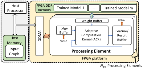
Figure 4. System design

Important Neighbor Identification (INI): INI (line 2 of Algorithm 2) is the key to achieve high accuracy with a Decoupled model. Following (Zeng et al., 2021), we use the Personalized PageRank (PPR) (Bahmani et al., 2010) score as the metric to indicate the importance of neighbor vertices w.r.t. a given target vertex. We use the local-push algorithm (Andersen et al., 2006) to compute approximate PPR scores. There are several benefits of using this approach: (1) As shown in (Zeng et al., 2021), PPR score is a good metric to reflect neighbor importance. Empirically, Decoupled models based on PPR achieve high accuracy with a small number of neighbor vertices (e.g., $100-200$ vertices) (Zeng et al., 2021). (2) The computation complexity of the local-push algorithm is low and remains low even when the input graph size grows (Aggarwal et al., 2021). (3) The local-push algorithm can be easily parallelized across multiple CPU cores.

3.3. System Design

Figure 4 depicts the proposed system for executing Algorithm 2.

Design Time: At design time, given the specification of the target FPGA platform and a set of Decoupled GNN models (see Section 4.5), we generate a single hardware accelerator and deploy it on the target FPGA platform. The overhead of generating the accelerator is a one-time cost. The trained GNN models are stored in the FPGA DDR memory. User can specify which model to use at runtime. On host platform, we develop the host program to run on the processor, which consists of three parts: (1) the subroutine for Important Neighbor Identification. (2) the subroutine (developed using Xilinx OpenCL (xil, [n.d.]a)) for allocating tasks on FPGA accelerator for a GNN model: it takes the specification of a GNN model and parameters (Section 4) of the accelerator as input, and performs task allocation on the accelerator. A task is a computation kernel (Section 4.1) of a GNN layer that will be executing by the accelerator. We develop a library for task allocation of the computation kernels in various GNN models. The subroutine searches for the library implementation based on the input GNN model at runtime. (3) the subroutine to perform data communication between CPU and FPGA.

Algorithm 3 Parallel Mini-batch Inference on CPU-FPGA

A batch of target vertices $\mathcal{V}_{t}$; A Decoupled GNN model specified by user (already trained and stored in FPGA DDR memory);

Node embeddings of target vertices: $\{\bm{h}_{v}^{L}:v\in\mathcal{V}_{t}\}$

while there is an idle CPU thread do $\triangleright$ CPU

    Pick a target vertex $v$ from $\mathcal{V}_{t}$ and remove $v$ from $\mathcal{V}_{t}$

    Extract important neighbors and build vertex-induced subgraph $\mathcal{G}^{\prime}(v)$

    Send vertex features and edges of $\mathcal{G}^{\prime}(v)$ to FPGA

while there is an idle PE do $\triangleright$ FPGA

    Load vertex features and edges of $\mathcal{G}^{\prime}(v)$ for a target vertex $v$

    for $l\leftarrow 1$ to $L$  do $\triangleright$ Inference using ACK

         for each $kernel$ from the $kernels$ of layer $l$  do

             Configure the execution mode of ACK for $kernel$

             Execute $kernel$ on ACK              

    Send embedding $\bm{h}_{v}^{L}$ back to CPU

Runtime: The overall execution process between CPU and FPGA is described in Algorithm 3. The input graph (including the edges and vertex features) is stored in the host memory. At runtime, the host processor receives the indices of a batch of target vertices and the GNN model specified by the user. On the host platform, the CPU runs the host program to perform important neighbor identification (line 2 of Algorithm 2) and constructs the vertex-induced subgraph for the target vertices. We use parallel threads on the CPU to execute the local-push algorithm (Aggarwal et al., 2021) for multiple target vertices concurrently. Then, the CPU extracts the features of input vertices and the edges of the subgraph, and sends them to the FPGA accelerator through the PCIe interconnection. The CPU also performs task allocation for the accelerator based on the specification of the GNN model. For example, for inferring a target vertex using a $L$-layer model with 2 kernels, the host program allocates $2L$ kernels for the accelerator to execute. On the FPGA platform, the input data from PCIe is directly sent to the accelerator through QDMA (xil, [n.d.]b). The FPGA accelerator consists of $N_{\text{pe}}$ parallel and independent processing elements (PEs), which can execute the forward propagation of $N_{\text{pe}}$ target vertices concurrently to obtain their embeddings. Adaptive Computation Kernel (ACK) executes the $L$-layer model layer-by-layer (see Algorithm 3). For each layer, the execution is performed kernel-by-kernel by ACK. To execute a kernel, the proper execution mode (see Section 4.2) of ACK is selected by setting the control bits of the hardware multiplexers in ACK. The overhead of such configuration is just one clock cycle.

4. Hardware Architecture

The proposed FPGA accelerator (Figure 4) consists of $N_{\text{pe}}$ parallel and independent processing elements (PEs). Each PE has an Adaptive Computation Kernel (ACK) to execute various computation kernels in GNNs, an Edge Buffer to store the edges, a Weight Buffer to store weight matrices, a Feature/Result Buffer to store the vertex features. The ACK of a PE contains 2-D mesh of ALUs (Section 4.2).

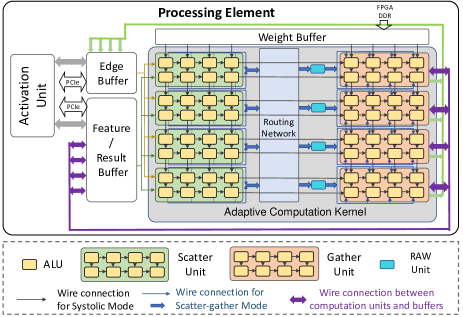
Figure 5. The details of a Processing Element

4.1. Computation Kernels of GNN

We summarize the various computation kernels in four widely used GNN models of the Decoupled version: GCN (Kipf and Welling, 2016), GraphSAGE (Hamilton et al., 2017), GIN (Xu et al., 2018), GAT (Veličković et al., 2017):

Feature Aggregation (FA): Feature Aggregation has two phases – Scatter phase and Gather phase. In Scatter phase, each vertex $v_{i}$ sends its features $\bm{h}_{i}$ through its outgoing edges in the vertex-induced subgraph to its neighbors. The vertex features are multiplied by the edge weight to generate the intermediate results. Then, in Gather phase, each vertex aggregates the incoming intermediate results through the $\text{aggregate}()$ function (e.g., element-wise Min, Max, Mean) to generate the aggregated features $\bm{z}_{i}$.

Feature Transformation (FT): After each vertex obtaining the aggregated feature vector $\bm{z}_{i}$, the aggregated features $\bm{z}_{i}$ are transformed through the $\text{update}()$ function. In the widely used GNN models (e.g. GCN, GraphSAGE, GIN, GAT), the $\text{update}()$ is a Multi-Layer Perceptron (MLP) with an element-wise activation function (e.g., ReLU, LeakyReLU).

Attention: Some GNN models (e.g., GAT) exploit the Attention mechanism to generate data-dependent edge weights. The weight of edge $e_{ij}$ is calculated based on ($\bm{h}_{i}$, $\bm{h}_{j}$, $\bm{W}_{\text{att}}$, $\bm{a}$). $\bm{W}_{\text{att}}$ is the attention weight matrix that is multiplied with $\bm{h}_{i}$ and $\bm{h}_{j}$. $\bm{a}$ is the vector that is multiplied with $\bm{W}_{\text{att}}\bm{h}_{i}||\bm{W}_{\text{att}}\bm{h}_{j}$ to get the edge weight $e_{ij}$.

While FT and Attention are dense computation kernels involving dense matrix multiplication, FA is the sparse computation kernel due to the sparsity and irregularity of the graphs. If we execute the different kernels using different hardware modules, the load imbalance can lead to hardware under-utilization and increased latency (See Section 4.3).

4.2. Hardware Modules

To address the load imbalance challenge, we propose Adaptive Computation Kernel (ACK) to execute various computation kernels of GNNs in a single hardware module.

Adaptive Computation Kernel (ACK): ACK contains an array of Arithmetic Logical Units (ALUs) of size $p_{\text{sys}}\times p_{\text{sys}}$. An ALU can execute various arithmetic operations including Multiplication, Addition, Multiply-Accumulation, Min, Max, etc. The proposed ACK has two execution modes – Systolic Mode and Scatter-Gather Mode – that can support FA, FT, Attention (Section 4.1).

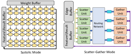
Figure 6. Two data paths realizing the dense (left) and sparse (right) execution modes of ACK

Systolic Mode: In Systolic Mode, the array of ALUs are organized as a two-dimension systolic array. Systolic array is an efficient architecture for dense matrix multiplication (Vucha and Rajawat, 2011), which has localized interconnections as shown in Figure 6. Systolic Mode supports dense matrix multiplication in FT and Attention.In Systolic Mode, ACK can execute the multiplication of weight matrix $\bm{W}$ and Feature matrix $\bm{H}_{\text{in}}$ (See Table 1, each row of $\bm{H}_{\text{in}}$ is a vertex feature vector $\bm{h}_{i}$) to obtain the output feature matrix $\bm{H}_{\text{out}}$. Weight Buffer streams the weight matrices of MLP (FT) or the attention weight matrix to the systolic array, and Feature/Result Buffer streams multiple vertex feature vectors into the systolic array. Systolic array of size $p_{\text{sys}}\times p_{\text{sys}}$ can execute $p_{\text{sys}}^{2}$ Multiply-Accumulation operations in each clock cycle. Both the Weight Buffer and the Feature Buffer have port width of $p_{\text{sys}}$ data, and can send $p_{\text{sys}}$ data to the systolic array in each clock cycle.

Scatter-Gather Mode: In Scatter-Gather Mode, the PE executes feature aggregation (FA) using Scatter-Gather paradigm (Algorithm 4). The array of ALUs is partitioned into multiple Scatter Units and Gather Units. In each Scatter Unit, the ALUs are organized as a vector multiplier that multiplies the vertex feature vector by the scalar edge weight. Similarly, in each Gather Unit, the ALUs execute the $\text{aggregate}()$ function. Suppose the feature vector has the format $\langle src,features\rangle$, where $src$ denotes the index of the source vertex and the $features$ is the feature vector of the source vertex. Edge has the format $\langle src,dst,weight\rangle$, where $src,dst,weight$ denote the source vertex index, destination vertex index, edge weight respectively. The generated intermediate results (updates) by the Scatter Units have the format $\langle dst,features\rangle$. For the vertex-induced subgraph containing $N$ vertices, the $N$ vertices are equally partitioned to the Gather Units. The routing network performs all-to-all interconnection between Scatter Units and Gather Units. It routes the immediate results $\langle dst,features\rangle$ generated by Scatter Units to the corresponding Gather Units based on the index $dst$. For example, suppose a Gather Unit is responsible for accumulating the results to vertices $v_{1}-v_{64}$. All immediate results that has $dst$ ranging from $1$ to $64$ will be routed to this Gather Unit. The routing network is implemented as a butterfly network (Choi et al., 2021) (See (Choi et al., 2021) for the details of the routing network).

Algorithm 4 Feature Aggregation using Scatter-Gather Paradigm

while not done do

    for each edge $e\langle src,dst,weight\rangle$  do $\triangleright$ Scatter Unit

         Produce update $u\leftarrow$Scatter($src.features,e.weight$)     

    for each update $u\langle dst,features\rangle$  do $\triangleright$ Gather Unit

         Update vertex $dst\leftarrow$ Gather($u.features$)     

To switch between the two execution modes, each ALU maintains multiplexers with control logic to select the input and output ports for an execution mode. When the execution of a kernel is completely finished, the ACK can start to execute the next kernel. In our design, there are $p_{\text{sg}}$ Scatter units and $p_{\text{sg}}$ Gather Units, where $p_{\text{sg}}$ is decided by $p_{\text{sg}}=p_{\text{sys}}/2$ . the Feature/Result Buffer have $p_{\text{sg}}$ banks. Each bank stores the feature vectors of the part of vertices in the vertex-induced subgraph (Algorithm 2). Each bank is connected to a Gather Unit. Each Scatter Unit or Gather Unit has $2p_{\text{sg}}$ ALUs. Note that read-after-write (RAW) data hazard may occur when accumulators in the Gather Unit read the old feature vertex vector from the Feature/Result Buffer. To resolve the RAW data hazard, we implement a RAW Unit before Gather Unit.

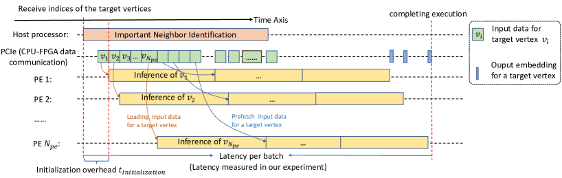
Figure 7. Task scheduling for mini-batch GNN inference on the CPU-FPGA platform

Activation Unit: The Activation Unit executes the element-wise activation function in FT and the Softmax function in Attention. These functions are implemented using Xilinx High-Level Synthesis (HLS) (O’Loughlin et al., 2014). For example, the Softmax function is implemented by using $\verb|hls::exp(x)|$ function as the building block.

Double/triple buffering: In a Processing Element, there are three Feature/Result Buffers for triple buffering. The first Buffer stores the vertex feature vectors of the current GNN layer. The second Buffer stores the vertex feature vectors of the next GNN layer. The third Buffer is used for prefetching the input vertex feature vectors of the next target vertex. Similarly, Edge Buffer is also designed with triple buffering. Weight buffer is implemented using double buffering, where one buffer is used for storing the weight matrix of the current layer, and the other buffer is used to store the weight matrix of the next layer. Through double/triple buffering, memory access and computation are overlapped to reduce the overall inference latency.

$\text{Readout}()$ function: the $\text{Readout}()$ function (Line 6 of Algorithm 2) has negligible computation complexity and it is executed by ACK in Scatter-Gather Mode.

4.3. Load Balance

The key benefit of our design is that we use a single hardware module (ACK) to execute various computation kernels with high efficiency. Therefore, we are able to assign all the on-chip computation resources to ACKs. In the hybrid accelerators (Yan et al., 2020; Zeng and Prasanna, 2020; Zhang et al., 2021), the computation resources are divided among different hardware modules to execute different computation kernels. Suppose for a single GCN layer, feature aggregatgion (FA) has the workload $\alpha_{1}$ $(\alpha_{1}>0)$ and feature transformation (FT) has the workload $\alpha_{2}$ $(\alpha_{2}>0)$, and the total computation resource is $\beta$. In our design, we use $\beta$ for ACKs. Therefore, the latency for executing this single GCN layer of our design is: $\frac{\alpha_{1}+\alpha_{2}}{\beta}$. In the hybrid accelerator, suppose the hardware module for FA uses $\beta_{1}$ resources and the hardware module for FT uses $\beta-\beta_{1}$ resources. The latency for executing this single GCN layer is $\max\left(\frac{\alpha_{1}}{\beta_{1}},\frac{\alpha_{2}}{\beta-\beta_{1}}\right)$. It can be proved that:

(1) $$\frac{\alpha_{1}+\alpha_{2}}{\beta}\leqslant\max\left(\frac{\alpha_{1}}{\beta_{1}},\frac{\alpha_{2}}{\beta-\beta_{1}}\right)\quad(\beta>0,\beta_{1}>0,\beta-\beta_{1}>0)$$

$\frac{\alpha_{1}+\alpha_{2}}{\beta}=\max\left(\frac{\alpha_{1}}{\beta_{1}},\frac{\alpha_{2}}{\beta-\beta_{1}}\right)$ when $\frac{\alpha_{1}}{\beta_{1}}=\frac{\alpha_{2}}{\beta-\beta_{1}}$. In the Decoupled GNN model, the workload of FA $\alpha_{1}$ is usually unpredictable because the number of edges in the receptive field depends on the connectivity of the input graph. Moreover, varying the receptive field size can vary the workload $\alpha_{1}$, $\alpha_{2}$ at different rate. Therefore, in a fixed hybrid accelerator, it is hard to keep load balance for various input graphs and Decoupled models with various receptive field sizes. The load imbalance incurs increased latency. To execute GNN models with more than two computation kernels (e.g., GAT), load imbalance can be more severe in hybrid accelerators.

4.4. Task Scheduling on CPU-FPGA

On the CPU-FPGA platform, the proposed task scheduling for performing inference on a batch of $C$ vertices using $N_{\text{pe}}$ parallel PEs ($C\gg N_{\text{pe}}$) is depicted in Figure 7. The scheduling is based on Algorithm 3. The host processor performs Important Neighbor Identification and builds a vertex-induced subgraph for each of the target vertices. If there is an idle PE, it loads the input vertex feature vectors of the vertex-induced subgraph for a target vertex. The PE also prefetches the input data for the next target vertex. After loading the input data, the PE executes the $L$-layer GNN forward propagation for the target vertex. Finally, the PE sends the embedding of the target vertex back to the host processor.

CPU-FPGA data communication: Using the proposed scheduling, the execution of the accelerator and the CPU-FPGA data movement are overlapped for all but the first vertex in a batch. Denote $t_{\text{initialization}}=t_{\text{load}}+t_{\text{INI}}$ as the initialization overhead of a batch, where $t_{\text{INI}}$ is the latency of runing INI for a vertex using a single CPU thread on the host processor. Suppose that the number of important vertices for the target vertex is $N$, the feature length is $f$, each vertex feature has $b_{\text{fe}}$ bits and each edge has $b_{\text{ed}}$ bits. The induced subgraph for a target vertex has at most $N(N-1)/2$ edges. This data communication overhead $t_{\text{load}}$ for loading the induced subgraph (vertex features; edges) for a target vertex can be approximated by:

(2) $$t_{\text{load}}\leq\frac{Nfb_{\text{fe}}+N(N-1)b_{\text{ed}}/2}{\text{PCIe Bandwidth}}+t_{\text{fixed}}$$

where $t_{\text{fixed}}$ is the fixed latency for initialing a data transfer through the PCIe interconnection which is usually $0.3-0.4\mu s$ (Neugebauer et al., 2018). In a Decoupled model, $N$ is small and is fixed. Thus, the above overhead is small. Note that $t_{\text{load}}$ does not increase with the depth of the GNN model. Compared with the computation complexity of the inference, the overhead of CPU-FPGA data communication is usually negligible (See Section 5.4). Thus, $t_{\text{initialization}}$ is negligible.

4.5. Design Space Exploration

We perform design space exploration (DSE) to determine the hardware parameters. The inputs to our DSE are (1) available hardware resources ($N_{\text{DSP}}$: number of DSPs) on FPGA, (2) arithmetic operations in the given set of Decoupled GNN models that needs to be supported. Given the inputs, the DSE determines the number of DSPs in a ALU $N_{\text{ALU}}$, the size of ACK in a PE $p_{\text{sys}}\times p_{\text{sys}}$, the number of PEs $N_{\text{pe}}$ in the accelerator. The proposed design has the following properties:

• The proposed accelerator can execute a GNN model as long as the ALU can support all the arithmetic operations (e.g., Min. Max, Add, Sub, etc) in this GNN model. $N_{\text{ALU}}$ is determined based on the arithmetic operations of a given Decoupled GNN model.

• The size of the ACK $p_{\text{sys}}\times p_{\text{sys}}$ in a PE determines the latency of inferring a single target vertex, and the number of PEs $N_{\text{pe}}$ decides how many target vertices can be inferred concurrently. Thus, the total on-chip computation resources should be exhausted by $N_{\text{pe}}\cdot p_{\text{sys}}^{2}$. The value of $N_{\text{pe}}$ depends on the batch size: for large batch sizes, both large and small $N_{\text{pe}}$ work well since sufficient parallelism is available across target vertices; for small batch sizes, it is desirable to set $N_{\text{pe}}$ as small in order to still achieve low latency per batch. Since batch sizes vary significantly in real-world applications, our DSE minimizes $N_{\text{pe}}$ by maximizing $p_{\text{sys}}\times p_{\text{sys}}$ in a PE.

• To efficiently implement Scatter Unit, Gather Unit and routing network in ACK on the target platform, the dimension of ACK $p_{\text{sys}}$ should be power of 2.

The above analysis leads to the following three-step DSE algorithm:

• Step 1: Determine $N_{\text{ALU}}$ based on all the arithmetic operations (given GNN models) to be supported.

• Step 2: Maximize the size of ALU array $p_{\text{sys}}$ in a PE: $p_{\text{sys}}=2^{\left\lfloor\log_{2}\sqrt{N_{\text{DSP}}/N_{\text{ALU}}}\right\rfloor}$

• Step 3: Determine the number of PEs: $N_{\text{pe}}=\left\lfloor\frac{N_{\text{DSP}}/N_{\text{ALU}}}{p_{\text{sys}}\times p_{\text{sys}}}\right\rfloor$

Many modern FPGAs have multiple Super Logic Regions (SLRs) with limited interconnection among SLRs. We perform the proposed three-step DSE for each Super Logic Region respectively. The proposed DSE has constant computation complexity and can be completed using a single CPU thread instantaneously. Note that the routing network has $p_{\text{sys}}/2$ input ports and $p_{\text{sys}}/2$ output ports with $(32\times p_{\text{sys}})$-bit data width. Its hardware cost is $\mathcal{O}(p_{\text{sys}}^{2}\log p_{\text{sys}})$ which also increases with $p_{\text{sys}}$. The step of maximizing $p_{\text{sys}}$ in our DSE may incur additional hardware overhead due to expanding the routing network. Fortunately, as shown in (Choi et al., 2021), even a large-scale 512-bit 32-input-32-output routing network only consumes less than 189$K$ LUTs, which is far smaller ($<18\%$) than the total LUTs of state-of-the-art FPGA boards. Since all computation is performed with ALU, as long as LUT consumption is $<100\%$ the latency won’t be affected. In the large-scale FPGA device, such as Alveo U200 and U250, $p_{\text{sys}}$ does not exceed 16. Therefore, the routing network is not the resource bottleneck in our design.

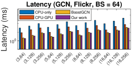
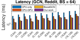
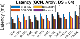
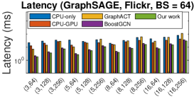
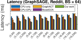
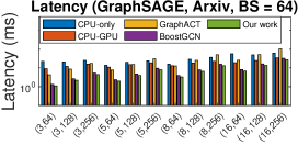
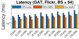
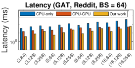
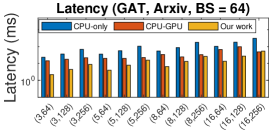
Figure 8. Comparison of inference latency (Batch size=64) for Decoupled GNN models with various depth and receptive field. Y-axis is in log-scale. X-axis denotes (number of layers $L$, size of receptive field $N$)

5. Experiments

5.1. Hardware Details and Baseline Platforms

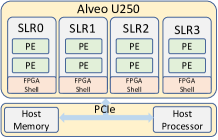
Figure 9. Proposed CPU-FPGA implementation with the accelerator design on a state-of-the-art FPGA board (Xilinx Alveo U250)

We use High-level Synthesis (HLS) to develop the hardware templates. The obtained hardware parameters through DSE are annotated into the developed hardware templates, and we use the vendor’s tool to synthesize the hardware design and generate the accelerator bitstream. Then, the bitstream is deployed on the target FPGA platform. We perform DSE to generate a hardware accelerator on a state-of-the-art FPGA platform (Xilinx Alveo U250) for three widely used GNN models (GCN, GraphSAGE, GAT). The FPGA is hosted by an Intel Xeon Gold 5120 CPU. Figure 9 depicts the generated system design (Figure 4) on the CPU-FPGA platform. Based on the arithmetic operation in the three GNN models, each ALU consumes 5 DSPs. The ACK in each PE has an ALU array of size $16\times 16$. In the ACK, there are 8 Scatter Units and 8 Gather Units. Each of the Scatter Units and Gather Units has an ALU array of size $2\times 8$. The routing network is a butterfly network of 8 input ports and 8 output ports. Each input/output port has 512-bit width. On Alveo U250, there are 8 PEs in four Super Logic Regions (SLRs) with each SLR having 2 PEs. The hardware synthesis and Place&Route are performed using Vitis 2021.1 (xil, [n.d.]c). The above accelerator on Alveo U250 consumes $762$K LUTs, $10854$ DSPs, $1853$ BRAMs and $1050$ URAMs. The resource utilization is reported after P&R. On the host processor, we use 8 threads to execute important neighbor identification. We deploy the host program on the host processor (Intel Xeon Gold 5120 CPU) and accelerator bitstream on the FPGA (Xilinx Alveo U250). The host processor and FPGA are connected through the PCIe $3.0\times 16$ which form our target CPU-FPGA platform. We execute the mini-batch inference on the target CPU-FPGA platform and measure the end-to-end latency using $\verb|chrono|$ library of C++.

Table 2. Specifications of platforms

Platforms CPU AMD Ryzen 3990x GPU Nvidia RTX3090 FPGA Alveo U250 Release Year 2020 2020 2018 Technology TSMC 7 nm TSMC 7 nm TSMC 16 nm Frequency 2.90 GHz 1.7 GHz 300 MHz Peak Performance 3.7 TFLOPS 36 TFLOPS 0.72 TFLOPS On-chip Memory 256 MB L3 cache 6 MB L2 cache 54 MB Memory Bandwidth 107 GB/s 15.6 GB/s (PCIe) 15.6 GB/s (PCIe)

Baseline Platforms: We compare the following platforms in our experiments: (1) Baseline 1: CPU-only platform (AMD Ryzen 3990x), (2) Baseline 2: CPU-GPU platform (Intel Xeon Gold 5120 CPU + Nvidia RTX3090), (3) Baseline 3: CPU-GraphACT (Intel Xeon Gold 5120 CPU + GraphACT (Zeng and Prasanna, 2020)), (4) Baseline 4: CPU-BoostGCN (Intel Xeon Gold 5120 CPU + BoostGCN (Zhang et al., 2021)), (5) Our work: CPU-FPGA (Intel Xeon Gold 5120 CPU + proposed accelerator). The specifications of various platforms are shown in Table 2 and Table 3. To execute mini-batch inference, the CPU-only platform uses Pytorch with Intel MKL as the backend and the CPU-GPU plaform uses the Pytoch library with CUDA as the backend. Note that GraphACT supports GraphSAGE only. BoostGCN can support GCN and GraphSAGE. However, BoostGCN needs to generate a separate FPGA bitstream for each GNN model.

Latency measurement: In the experiments, we measure the latency per batch defined in Section 3.1 and Figure 7. For all the baselines and our work, the measured latency per batch is the duration from the time when host processor receives the of indices of a batch of target vertices to the time when inference for all the vertices have been completed. The overhead of Important Neighbor Identification and the data movement between CPU and GPU/FPGA through PCIe are included in our measured latency.

Table 3. Platform specifications of GNN accelerators

GraphACT (Zeng and Prasanna, 2020) This paper BoostGCN (Zhang et al., 2021) Platform Xilinx Alveo U200 Xilinx Alveo U250 Intel Stratix 10 GX Frequency 300 MHz 300 MHz 250 MHz Data format Float32 Float32 Float32 Peak Performance 249.6 GFLOPS 614 GFLOPS 640 GFLOPS On-chip Memory 35.8 MB 45 MB 32 MB Memory Bandwidth 15.6 GB/s (PCIe) 15.6 GB/s (PCIe) 15.6 GB/s (PCIe)

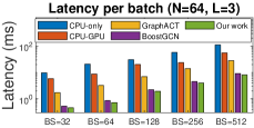
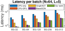
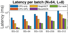
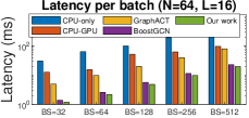
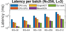
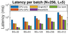
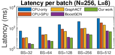
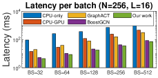
Figure 10. Latency under various batch sizes (BS) for GraphSAGE and Flickr dataset

5.2. Benchmarks

Table 4. Dataset Statistics

Dataset Vertices Edges Features $f_{\text{in}}$ Classes Degree Flickr (FL) (Zeng et al., 2020) 89,250 899,756 500 7 10 Reddit (RE) (Hamilton et al., 2017) 232,965 116,069,191 602 41 50 ogbn-arxiv (OA) (Hu et al., 2020) 169,343 1,166,243 128 7 40

We evaluate various Decoupled Models (GCN, GraphSAGE, GAT) that can achieve superior accuracy. As shown in (Zeng et al., 2021), the Decoupled Models ($N<200$ and $L=3$ or $5$) can already achieve higher accuracy than the original Coupled GNN models (GCN, GraphSAGE, GAT). The Decoupled Models can achieve higher accuracy when $L$ is increased. To evaluate Decoupled models with various $L$ and $N$, we set the hidden dimension of each GNN layer as $f_{l}=256,(1\leqslant l\leqslant L)$ following (Zeng et al., 2021). We set the number of layers $L$ as $3$, $5$, $8$, $16$ respectively. We specify the size of the receptive field $N$ as $64$, $128$, $256$. As shown in (Gupta et al., 2020), recommendation systems typically use batch size $64$, $128$, $256$. We evaluate our design using a wider range of batch sizes $32$, $64$, $128$, $256$, $512$. We use three representative graph datasets for evaluation as listed in Table 4.

5.3. Comparison with State-of-the-art

We show the comparison results (latency per batch) using various GNN models, $L$ and $N$ in Figure 8. Our CPU-FPGA implementation achieves $21.4-50.8\times$, $2.9-21.6\times$, $4.7\times$, $1.2\times$ speedup compared with CPU-only, CPU-GPU, CPU-GraphACT, and CPU-BoostGCN, respectively. Note that BoostGCN does not support GAT and needs to generate an accelerator for each GNN model.

On the CPU-only platform, the processor can directly (without PCIe overhead) access data from the host memory and the processor has large shared L3 cache. However, the feature aggregation of GNN results in irregular memory access pattern and low data reuse. The processor has limited L1 (32 KB) and L2 (512 KB) cache. The data exchange (vertex features;weight matrices;edges) among L1 cache, L2 cache, and L3 cache becomes the performance bottleneck and results in reduced sustained performance. For example, on multi-core platform, loading data from L3 cache incurs latency of $32$ns and loading data from L2 cache incurs latency of $5-12$ns. Compared with the CPU, the ACK in our accelerator can access data in one clock cycle during the inference execution.

For the CPU-GPU platform, although the GPU has higher peak performance, the GPU has higher latency than our CPU-FPGA platform because: (1) GPU has extra latency of loading data from host memory to GPU global memory and loading data from GPU global memory to GPU on-chip memory, while in our CPU-FPGA implementation, the FPGA accelerator can directly load data to the on-chip memory through QDMA from the host memory. (2) Similar to CPU, GPU has limited private L1 cache size (32 KB), therefore data exchange (vertex features;weight matrices;edges) between L2 cache and L1 cache becomes the performance bottleneck.

We compare our CPU-FPGA implementation with GraphACT (Baseline 3) and BoostGCN (Baseline 4) . GraphACT is optimized for subgraph-based mini-batch training which has similar computation pattern as the mini-batch inference of Decoupled GNN models. BoostGCN is the state-of-the-art FPGA accelerator for full-graph inference. Compared with CPU-GraphACT and CPU-BoostGCN, our CPU-FPGA implementation achieves lower latency because (1) our proposed ACK can efficiently execute various kernels in GNN. GraphACT and BoostGCN follow the hybrid design that two hardware modules are initialized for feature aggregation and feature transformation, respectively. The load imbalance of the two modules leads to hardware under-utilization on GraphACT and BoostGCN. (2) We adopt the Scatter-Gather paradigm to achieve massive computation parallelism for feature aggregation. GraphACT has limited computation parallelism in its Feature Aggregation Module.

Latency under various batch size: We compare the mini-batch inference latency with other platforms under various batch size. Figure 10 shows the experiment results using Flickr dataset. We use the GraphSAGE model. We only show these results due to the space limitation and the observation under other experimental settings is similar. Under various batch sizes, our CPU-FPGA implementations still achieve significantly lower latency than the CPU-only platform, CPU-GPU platform, CPU-GraphACT and CPU-BoostGCN.

5.4. Analysis of Execution Time

We perform a detailed analysis of the total execution time using the Xilinx Runtime (XRT) profiler to analyze the execution time of our CPU-FPGA implementation. Xilinx XRT can perform fine-grained profiling for the execution time of host program, data transfer between CPU and FPGA, and the execution time of the computation kernels on the FPGA.

Initialization overhead $t_{\text{initialization}}$: We measure the initialization overhead in our task scheduling (Figure 7). We use the results in Figure 11 for illustration since other experimental settings have similar results. The initialization overhead is $0.5\%-6\%$ of the total execution time, which is negligible.

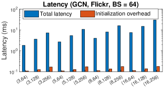
Figure 11. Comparison of the initialization overhead and total inference latency under various settings

Table 5. Average latency of loading the input data for a target vertex through PCIe interconnection

Flickr obgn-arxiv Reddit $N=64$ $12.6$ $\mu s$ $3.5$ $\mu s$ $15.1$ $\mu s$ $N=128$ $29.1$ $\mu s$ $7.7$ $\mu s$ $32.3$ $\mu s$ $N=256$ $72.5$ $\mu s$ $17.1$ $\mu s$ $72.7$ $\mu s$

Overhead of CPU-FPGA data communication: To perform inference on a target vertex, the feature vectors of its $N$ important neighbors and the edges in the induced subgraph are loaded from the host memory to the on-chip memory of a PE through PCIe. Note that the input data are directly sent to the on-chip memory through the QDMA. As shown in Table 5, we measure the average latency for loading the input data for a target vertex through PCIe. The above latency is hidden by our task scheduling for most target vertices (See Figure 7).

Table 6. Overhead of INI ($t_{\text{INI}}$)

Flickr ogbn-arxiv Reddit Time per vertex ($\mu s$) $96$ $37.6$ $87.1$

Overhead of INI ($t_{\text{INI}}$): On the host platform, we use 8 threads to execute INI. The measured overhead of INI $t_{\text{INI}}$ is shown in Table 6. Note that the measured overhead $t_{\text{INI}}$ is the time of INI for a vertex using single CPU thread on the host processor. The host processor can execute INI for 8 vertices concurrently. The average latency of INI is negligible compared with the total latency of mini-batch inference ($2-100$ ms). Moreover, The overhead $t_{\text{INI}}$ for most vertices is hidden by our task scheduling (See Figure 7).

6. Conclusion

In this paper, we proposed a novel hardware accelerator design to achieve low-latency mini-batch inference on CPU-FPGA heterogeneous platform. On various GNN models, we achieved load-balance and high hardware utilization via the novel Adaptive Computation Kernel design. As a result, our CPU-FPGA implementation with a single hardware accelerator (generated by our fast design space exploration algorithm) achieves significant latency reduction under various GNN models and batch sizes, compared with state-of-the-art CPU, CPU-GPU and CPU-FPGA implementations. In the future, we plan to extend our design to a model-architecture co-design framework, such that both accuracy and latency are optimized via jointly generating the configurations of model depth, receptive field size and hardware modules.

References

- (1)
- xil ([n.d.]a) [n.d.]a. Xilinx OpenCL Library. https://www.xilinx.com/html_docs/xilinx2017_4/sdaccel_doc/lyx1504034296578.html
- xil ([n.d.]b) [n.d.]b. Xilinx QDMA IP. https://www.xilinx.com/products/intellectual-property/pcie-qdma.html
- xil ([n.d.]c) [n.d.]c. Xilinx Vitis 2021.1. https://www.xilinx.com/support/documentation-navigation/design-hubs/2021-1/dh0089-vitis-embedded.html
- Aggarwal et al. (2021) Madhav Aggarwal, Bingyi Zhang, and Viktor Prasanna. 2021. Performance of Local Push Algorithms for Personalized PageRank on Multi-core Platforms. In HiPC 2021. IEEE, 370–375.
- Andersen et al. (2006) Reid Andersen, Fan Chung, and Kevin Lang. 2006. Local graph partitioning using pagerank vectors. In 2006 47th Annual IEEE Symposium on Foundations of Computer Science (FOCS’06). IEEE, 475–486.
- Bahmani et al. (2010) Bahman Bahmani, Abdur Chowdhury, and Ashish Goel. 2010. Fast incremental and personalized pagerank. arXiv preprint arXiv:1006.2880 (2010).
- Choi et al. (2021) Young-kyu Choi, Yuze Chi, Weikang Qiao, Nikola Samardzic, and Jason Cong. 2021. Hbm connect: High-performance hls interconnect for fpga hbm. In The 2021 ACM/SIGDA International Symposium on Field-Programmable Gate Arrays.
- Gallicchio and Micheli (2020) Claudio Gallicchio and Alessio Micheli. 2020. Fast and deep graph neural networks. In Proceedings of the AAAI Conference on Artificial Intelligence, Vol. 34.
- Geng et al. (2020) Tong Geng, Ang Li, Runbin Shi, Chunshu Wu, Tianqi Wang, Yanfei Li, Pouya Haghi, Antonino Tumeo, Shuai Che, Steve Reinhardt, et al. 2020. AWB-GCN: A graph convolutional network accelerator with runtime workload rebalancing. In 2020 53rd Annual IEEE/ACM International Symposium on Microarchitecture (MICRO). IEEE, 922–936.
- Geng et al. (2021) Tong Geng, Chunshu Wu, Yongan Zhang, Cheng Tan, Chenhao Xie, Haoran You, Martin Herbordt, Yingyan Lin, and Ang Li. 2021. I-GCN: A graph convolutional network accelerator with runtime locality enhancement through islandization. In MICRO-54: 54th Annual IEEE/ACM International Symposium on Microarchitecture. 1051–1063.
- Gupta et al. (2020) Udit Gupta, Carole-Jean Wu, Xiaodong Wang, Maxim Naumov, Brandon Reagen, David Brooks, Bradford Cottel, Kim Hazelwood, Mark Hempstead, Bill Jia, et al. 2020. The architectural implications of facebook’s dnn-based personalized recommendation. In 2020 IEEE International Symposium on High Performance Computer Architecture (HPCA). IEEE, 488–501.
- Hamilton et al. (2017) William L Hamilton, Rex Ying, and Jure Leskovec. 2017. Inductive representation learning on large graphs. In Proceedings of the 31st International Conference on Neural Information Processing Systems. 1025–1035.
- Hu et al. (2020) Weihua Hu, Matthias Fey, Marinka Zitnik, Yuxiao Dong, Hongyu Ren, Bowen Liu, Michele Catasta, and Jure Leskovec. 2020. Open graph benchmark: Datasets for machine learning on graphs. arXiv preprint arXiv:2005.00687 (2020).
- Kipf and Welling (2016) Thomas N Kipf and Max Welling. 2016. Semi-supervised classification with graph convolutional networks. arXiv preprint arXiv:1609.02907 (2016).
- Lerer et al. (2019) Adam Lerer, Ledell Wu, Jiajun Shen, Timothee Lacroix, Luca Wehrstedt, Abhijit Bose, and Alex Peysakhovich. 2019. Pytorch-biggraph: A large-scale graph embedding system. arXiv preprint arXiv:1903.12287 (2019).
- Li et al. (2021) Guohao Li, Matthias Müller, Guocheng Qian, and Bernard Perez. 2021. Deepgcns: Making gcns go as deep as cnns. IEEE Transactions on Pattern Analysis and Machine Intelligence (2021).
- Liang et al. (2020) Shengwen Liang, Cheng Liu, Ying Wang, Huawei Li, and Xiaowei Li. 2020. DeepBurning-GL: an automated framework for generating graph neural network accelerators. In 2020 ICCAD. IEEE, 1–9.
- Lin et al. (2021) Yi-Chien Lin, Bingyi Zhang, and Viktor Prasanna. 2021. HP-GNN: Generating High Throughput GNN Training Implementation on CPU-FPGA Heterogeneous Platform. arXiv preprint arXiv:2112.11684 (2021).
- Mernyei and Cangea (2020) Péter Mernyei and Cătălina Cangea. 2020. Wiki-cs: A wikipedia-based benchmark for graph neural networks. arXiv preprint arXiv:2007.02901 (2020).
- Neugebauer et al. (2018) Rolf Neugebauer, Gianni Antichi, José Fernando Zazo, Yury Audzevich, Sergio López-Buedo, and Andrew W Moore. 2018. Understanding PCIe performance for end host networking. In Proceedings of the 2018 Conference of the ACM Special Interest Group on Data Communication. 327–341.
- O’Loughlin et al. (2014) Declan O’Loughlin, Aedan Coffey, Frank Callaly, Darren Lyons, and Fearghal Morgan. 2014. Xilinx vivado high level synthesis: Case studies. (2014).
- Veličković et al. (2017) Petar Veličković, Guillem Cucurull, Arantxa Casanova, Adriana Romero, Pietro Lio, and Yoshua Bengio. 2017. Graph attention networks. (2017).
- Vucha and Rajawat (2011) Mahendra Vucha and Arvind Rajawat. 2011. Design and FPGA implementation of systolic array architecture for matrix multiplication. International Journal of Computer Applications 26, 3 (2011), 18–22.
- Xu et al. (2018) Keyulu Xu, Weihua Hu, Jure Leskovec, and Stefanie Jegelka. 2018. How powerful are graph neural networks? arXiv preprint arXiv:1810.00826 (2018).
- Yan et al. (2020) Mingyu Yan, Lei Deng, Xing Hu, Ling Liang, Yujing Feng, Xiaochun Ye, Zhimin Zhang, Dongrui Fan, and Yuan Xie. 2020. Hygcn: A gcn accelerator with hybrid architecture. In 2020 IEEE International Symposium on High Performance Computer Architecture (HPCA). IEEE, 15–29.
- Yang (2019) Hongxia Yang. 2019. Aligraph: A comprehensive graph neural network platform. In Proceedings of the 25th ACM SIGKDD International Conference on Knowledge Discovery & Data Mining. 3165–3166.
- Ying et al. (2018) Rex Ying, Jiaxuan You, Christopher Morris, Xiang Ren, William L Hamilton, and Jure Leskovec. 2018. Hierarchical graph representation learning with differentiable pooling. arXiv preprint arXiv:1806.08804 (2018).
- Zeng and Prasanna (2020) Hanqing Zeng and Viktor Prasanna. 2020. GraphACT: Accelerating GCN training on CPU-FPGA heterogeneous platforms. In Proceedings of the 2020 ACM/SIGDA International Symposium on Field-Programmable Gate Arrays. 255–265.
- Zeng et al. (2021) Hanqing Zeng, Muhan Zhang, Yinglong Xia, Ajitesh Srivastava, Andrey Malevich, Rajgopal Kannan, Viktor Prasanna, Long Jin, and Ren Chen. 2021. Decoupling the Depth and Scope of Graph Neural Networks. Advances in Neural Information Processing Systems 34 (2021).
- Zeng et al. (2020) Hanqing Zeng, Hongkuan Zhou, Ajitesh Srivastava, Rajgopal Kannan, and Viktor Prasanna. 2020. GraphSAINT: Graph Sampling Based Inductive Learning Method. In International Conference on Learning Representations.
- Zhang et al. (2021) Bingyi Zhang, Rajgopal Kannan, and Viktor Prasanna. 2021. BoostGCN: A Framework for Optimizing GCN Inference on FPGA. In 2021 IEEE 29th Annual International Symposium on Field-Programmable Custom Computing Machines (FCCM). IEEE, 29–39.
- Zhang et al. (2020) Bingyi Zhang, Hanqing Zeng, and Viktor Prasanna. 2020. Hardware acceleration of large scale GCN inference. In 2020 IEEE 31st International Conference on Application-specific Systems, Architectures and Processors (ASAP). IEEE, 61–68.
- Zhang and Chen (2018) Muhan Zhang and Yixin Chen. 2018. Link prediction based on graph neural networks. Advances in Neural Information Processing Systems 31 (2018).