ComENet: Towards Complete and Efficient Message Passing for 3D Molecular Graphs

Abstract

Many real-world data can be modeled as 3D graphs, but learning representations that incorporates 3D information completely and efficiently is challenging. Existing methods either use partial 3D information, or suffer from excessive computational cost. To incorporate 3D information completely and efficiently, we propose a novel message passing scheme that operates within 1-hop neighborhood. Our method guarantees full completeness of 3D information on 3D graphs by achieving global and local completeness. Notably, we propose the important rotation angles to fulfill global completeness. Additionally, we show that our method is orders of magnitude faster than prior methods. We provide rigorous proof of completeness and analysis of time complexity for our methods. As molecules are in essence quantum systems, we build the complete and efficient graph neural network (ComENet) by combing quantum inspired basis functions and the proposed message passing scheme. Experimental results demonstrate the capability and efficiency of ComENet, especially on real-world datasets that are large in both numbers and sizes of graphs. Our code is publicly available as part of the DIG library (https://github.com/divelab/DIG).

1 Introduction

In machine learning, structured objects such as molecules [14, 55, 54], proteins [9, 16, 35, 39, 30], materials [56], and quantum systems [33, 17] are usually modeled as graphs. Original modeling shows basic connections between units and the resulted data type is known as 2D graphs. Accordingly, 2D graph neural networks (GNNs) have been intensively studied [14, 21, 20, 57, 61, 34] and the message passing scheme [24, 7, 53] is shown effective to realize 2D GNNs. However, in the modern machine learning era, it is increasingly accepted that modeling real-world data like molecules as 2D graphs leads to inborn defects for succeeding learning models. In practice, 3D information is crucial, based on which some important geometries can be derived, such as chemical bond lengths in molecular modeling. This essentially raises the need of a new data type, known as 3D graphs.

Formally, a 3D graph contains the original 2D graph as well as Cartesian coordinates for all nodes. In this work, we follow invariant 3D GNNs [45, 22, 32, 47, 36, 23] that take relative 3D information, like distances and angles, as inputs to networks. Such relative geometries are naturally SE(3)-invariant. The main challenge comes from what geometries should be computed such that 3D information is incorporated completely. A most recent work SphereNet [36] shows that distance, angle, and torsion information is necessary to incorporate more comprehensive 3D information. However, SphereNet is only complete in local neighborhood, failing to achieve global completeness and distinguish a wide range of molecular structures such as conformers. Let $n$ and $k$ denote the number of nodes and the average degree in a 3D graph. Existing methods also exhibit excessive time complexity of $O(nk^{2})$ or even $O(nk^{3})$, severely preventing their scalability in real-world applications.

In this work, we propose ComENet as a complete and efficient graph neural network for 3D molecular graph learning. We first formally provide the definition of completeness. Intuitively, a geometric transformation is considered as complete if it generates distinct representations for any two different 3D graphs. Based on this, we propose a novel message passing scheme by faithfully fulfilling global completeness via the important rotation angles. In addition, we design novel strategies to achieve local completeness, largely reducing the computing complexity to $O(nk)$. To elucidate the merits of the proposed methods, we provide rigorous proof of geometric completeness achieved by our method. Combining the novel message passing scheme and quantum inspired features, ComENet is developed for 3D molecular graphs. We apply ComENet to two large-scale datasets including OC20 and Molecule3D, and a commonly used dataset QM9. Experiments show that ComENet performs similar to existing best methods, but accelerates the training and inference by 6-10 times on various datasets. We summarize the contributions of ComENet as below. (i). To our best knowledge, it is the first rigorously complete pipeline for 3D molecular graph learning. Theoretically, it is guaranteed to incorporate 3D information completely without information loss. Practically, it can distinguish all molecular structures in nature. (ii). It is highly efficient. The message passing is shown to be orders of magnitude faster than existing methods in terms of time complexity. (iii). The great capability and efficiency of ComENet allow its scalability to real-world molecule datasets that are large in both numbers and sizes of graphs. (iv). It achieves similar or better performance compared with existing methods, and dramatically accelerates the training and inference by 6-10 times.

Relations with Prior Work. SphereNet [36] is a recent method that achieves local completeness with a complexity of $O(nk^{2})$. In summary, SphereNet is not complete and not efficient enough for processing large-scale molecular graphs. However, ComENet is complete and much more efficient with a complexity of $O(nk)$. Technically, a primary difference is that, ComENet proposes to use the important rotation angles to achieve global completeness. As a result, ComENet is provably complete as shown in Sec. 2.2. Practically, ComENet is able to identify a wide range of real-world structures such as conformers, achieving completeness at the conformer level, as introduced in Sec. 2.3. In addition, ComENet and SphereNet both use $(d,\theta,\phi)$ in the spherical coordinate system (SCS) to obtain local completeness. Indeed, the fact that $(d,\theta,\phi)$ can specify the location of a point in SCS is widely known. The key difference lies in that, SphereNet operates within 2-hop neighborhood, while ComENet operates within 1-hop neighborhood. When coupled with rotation angles, ComENet can achieve provable completeness with a reduced complexity of $O(nk)$. This different message passing for local completeness in ComENet entails many differences with SphereNet, including building coordinate systems, defining $z$-axis, choosing reference nodes, and computing $(d,\theta,\phi)$, as detailed in Sec. 2.4. All the computing procedures for ComeNet are described in detail in Algorithm 1 of Appendix A.1.

2 The Proposed Message Passing Scheme

2.1 Notations & Definitions

We first formally define notations and the concept of completeness used in this paper.

Notations. A 3D graph $G$ can be represented as $G=(V,A,P)$. The node feature matrix $V=[\textbf{v}_{1},\textbf{v}_{2},\cdot\cdot\cdot,\textbf{v}_{n}]^{T}\in\mathbb{R}^{n\times d_{v}}$ with each $\textbf{v}_{i}\in\mathbb{R}^{d_{v}}$. The adjacency matrix $A\in\mathbb{R}^{n\times n}$, based on which we additionally define there is an edge $e_{ij}$ if $A[i][j]=1$. The position matrix $P=[\textbf{p}_{1},\textbf{p}_{2},\cdot\cdot\cdot,\textbf{p}_{n}]^{T}\in\mathbb{R}^{n\times 3}$, where $\textbf{p}_{i}=(x_{i},y_{i},z_{i})\in\mathbb{R}^{3}$ is the position vector for node $i$ given in the Cartesian coordinate system (CSC). The relative position $\textbf{p}_{ij}$ of node $j$ to node $i$ is defined as $\textbf{p}_{ij}=\textbf{p}_{j}-\textbf{p}_{i}$. Particularly, throughout this paper, we define $k$ as the average degree for $G$.

We then formally define completeness given a geometric transformation $\mathcal{T}$. In particular, we aim at incorporating 3D information in 3D molecular graphs. Hence, our definition of completeness is set from the geometric view. Generally, $\mathcal{T}$ maps a 3D graph $G=(V,A,P)$ to a geometric representation with size $m\times h$, where $m$ is the number of transformed geometric features and $h$ is the feature size. $\mathcal{T}$ can be different dependent on different methods, resulting in different $m\in\mathbb{N}^{+}$ or $h\in\mathbb{N}^{+}$. For example, SchNet [45] only computes the distance for each edge based on the coordinates of the two nodes connected by this edge. Thus, SchNet maps $G$ to a representation with size $m\times h$, where $m$ is the number of edges in $G$ and $h=1$. However, such geometric transformation is not complete. We provide the definition of completeness as below:

Definition 1 (Completeness).

For two 3D graphs $G_{1}=(V,A,P_{1})$ and $G_{2}=(V,A,P_{2})$, a geometric transformation $\mathcal{T}:(\mathbb{R}^{n\times d_{v}},\mathbb{R}^{n\times n},\mathbb{R}^{n\times 3})\mapsto\mathbb{R}^{m\times d}$ is considered as complete when

$$\mathcal{T}(G_{1})=\mathcal{T}(G_{2})\iff\exists R\in\mathrm{SE(3)},P_{1}=R(P_{2}).$$

Here $\mathrm{SE(3)}$ denotes the Special Euclidean group in 3 dimensions. It include all rotations and translations in 3D [1, 26, 36, 43]. Thus $R$ is a transformation that combines rotation and translation. A rotation transformation can be represented with a $3\times 3$ rotation matrix, and a translation transformation can be represented by a $3\times 1$ vector. Matrix form of $\mathrm{SE(3)}$ is provided in Appendix A.2. The reason why we introduce $\mathrm{SE(3)}$ lies in that, a combination of rotation and translation will not change the 3D conformation of a 3D graph. In Def. 1, if $P_{1}$ and $P_{2}$ are in the same $\mathrm{SE(3)}$ group, then $G_{1}$ and $G_{2}$ would share the same 3D conformation. As a result, $G_{1}$ and $G_{2}$ would be the same 3D graph. Intuitively, a complete geometric transformation $\mathcal{T}$ can distinguish any two different 3D graphs. This is to say, as long as two 3D graphs differ in 3D conformations, their outputs from $\mathcal{T}$ would be different.

2.2 Global Completeness via Rotation Angles

Existing studies focus on the complete representation learning of local neighborhood. Earlier methods like SchNet [45] and DimeNet [22] cannot achieve local completeness. In a more recent method SphereNet, completeness is guaranteed within edge-based 1-hop local neighborhood, but fails to hold in the whole 3D graph. In this section, we move a step forward to formally fulfill global completeness for a given 3D molecular graph. Particularly, for the purpose of clear illustration, we safely assume local completeness is already obtained by exiting methods like SphereNet.

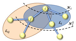
(a) Illustration of a 2-hop local structure.

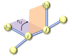
(b) Illustration of computing the rotation angle for an edge $e_{ij}$.

Figure 1: Illustrations of how to achieve global completeness in our proposed methods.

Without loss of generality, we start by describing our method to attain full completeness within 2-hop neighborhood, as illustrated in Fig. 1LABEL:sub@fig:two-hop. Formally, for a center node $i$, we let $\mathcal{N}_{i}$ and $\mathcal{N}^{2}_{i}$ denote two sets of indices of $i$’s 1-hop and 2-hop neighboring nodes, respectively. We also define any node $i$ and its 1-hop neighborhood as a local structure. Then the whole 2-hop neighborhood of node $i$ can be viewed as $1+|\mathcal{N}_{i}|$ local structures centered in $i$ and $\mathcal{N}_{i}$, defined as $\mathcal{L}_{i}$ and $\mathcal{L}_{ij,j\in\mathcal{N}_{i}}$, respectively. As shown in Fig. 1LABEL:sub@fig:two-hop, $\mathcal{L}_{i}$ is the local structure centered in $i$, and $\mathcal{L}_{ij}$ is the local structure centered in $j$. Apparently, each local structure $\mathcal{L}_{ij,j\in\mathcal{N}_{i}}$ shares the common edge $e_{ij}$ with the local structure $\mathcal{L}_{i}$. Given the complete representation for each local structure, for the structure $\mathcal{L}_{i}\cup\mathcal{L}_{ij}$, the only remaining degree of freedom is the rotation angle of edge $e_{ij}$, denoted as $\tau_{ij}$. With the rotation angles for all the $|\mathcal{N}_{i}|$ common edges specified, we can obtain a complete representation for 2-hop neighborhood of node $i$. Achieving completeness beyond 2-hop neighborhood is similar. Overall, after considering rotation angles, the global completeness can be easily guaranteed when it gradually generalizes from $n$- to $(n+1)$-hop neighborhood.

Essentially, each edge in an input graph can be treated as a common edge between different local structures. We reveal how to compute the rotation angle $\tau_{ij}$ for each edge $e_{ij}$ in Fig. 1LABEL:sub@fig:torsion. Specifically, we choose two reference nodes whose indices are $f_{i\backslash j}$ and $f_{j\backslash i}$ for node $i$ and $j$, respectively. $f_{i\backslash j}$ denotes the index of $i$’s nearest neighboring node except $j$, and $f_{j\backslash i}$ denotes $j$’s nearest neighboring node except $i$. Then $\tau_{ij}$ for edge $e_{ij}$ is the angle from the plane formed by $f_{i\backslash j},i,j$ to the plane formed by $i,j,f_{j\backslash i}$. As analyzed previously, the global conformation of the input graph can be identified based on all local structures and rotation angles. As a result, given fixed local structures, the global completeness the input 3D molecular graph is fulfilled by additionally considering the rotation angle of each edge, as introduced in this section. Note that in terms of the selection of reference nodes for computing a rotation angle, we think a selection strategy is valid as long as it is applied to every edge consistently. In this work, for an edge $e_{ij}$, we choose the nearest neighboring nodes for $i$ and $j$ as reference nodes, which are $f_{i\backslash j}$ and $f_{j\backslash i}$, respectively. We apply this selection strategy to all edges in a 3D graph for computing corresponding rotation angles. With such selection strategy, we can prove that our method is complete as shown in Sec. 3.1. We also show in Appendix A.3 that it is easier to prove completeness using nearest neighboring nodes as reference nodes.

2.3 Rotation Angles for Conformer Identification

The proposed rotation angles in Sec. 2.2 play a crucial role in identifying some important molecular structures, such as conformers. In nature, a real molecule exits as an ensemble of interconventing 3D structures, known as conformers [5, 4, 19]. Different conformers posses the same 2D molecular graph, but differ in 3D structures. Generally, a conformer for a molecule exits with a certain probability and may exhibit distinct properties [5, 4]. As shown in Fig. 2(a), different conformers for the molecule butane ($\text{C}_{4}\text{H}_{10}$) show varying conformation energy. To this end, it is important to design complete 3D GNNs for identifying molecules at the conformer level. From the geometry perspective of view, a conformer distinguishes itself from others mainly through varying rotation angles of chemical bonds [19]. As shown in Fig. 2(b), given the fixed ethyl (-$\text{C}_{2}\text{H}_{5}$) of both sides, the only degree of freedom is the rotation angle of the C-C bond. In literature, the ethyl is formulated as a local 3D graph. Existing studies focus on the complete representation of such local structures, failing to identify the whole 3D graph globally. Essentially, they can only distinguish different molecules, trying to achieve completeness at the molecule level rather that the finer comformer level. By integrating the rotation angles as in Sec. 2.2 into the message passing scheme, our methods can fulfill rigorous completeness at the conformer level and can distinguish all conformers in nature.

Figure 2: (a). Illustration that the relative conformation energy of butane is a function of the rotation angle of the C-C bond. (b). A 3D view of the four conformers in (a).

2.4 Local Completeness with Improved Efficiency

Formally, each node and its local neighborhood can be viewed as a local structure. Existing studies focus on the learning of local structures and SphereNet achieves local completeness. However, SphereNet induces the complexity of $O(nk^{2})$, restricting its scalability on large molecules in practice. Here, we design a novel strategy to guarantee local completeness with the computing cost of $O(nk)$.

Specifically, we follow SphereNet and perform on the spherical coordinate system. It is commonly known that the location of each node can be completely determined using the tuple $(d,\theta,\phi)$ in SCS. SphereNet employs the directional message passing (DMP) fashion that operates within 2-hop neighborhood. It first updates messages over edges thus the center edge is $z$-axis in SCS. For node $i$, the computing of the tuple $(d,\theta,\phi)$ involves 2-hop information. However, we view 1-hop neighborhood as a local structure, which requires all strategies in our local completeness to be different from SphereNet, including building local coordinate systems, defining z-axis, picking reference nodes, and computing $(d,\theta,\phi)$. First, we build a light local coordinate system for any node $i$’s corresponding local structure. Similarly, the center node $i$ serves as the origin. Then $z$-axis is defined as the direction from $i$ to its nearest neighbor $f_{i}$, and $xz$-plane is further formed by $z$-axis and $i$’s second nearest neighbor $s_{i}$. Finally, the tuple $(d,\theta,\phi)$ is computed within 1-hop neighborhood with a complexity of $O(nk)$. Particularly, we analyze efficiency versus model expressiveness in Sec. 3.2. We show that compared with the DMP fashion used by SphereNet, our method operating within 1-hop neighborhood hurts the model expressiveness a bit by largely improves the efficiency.

2.5 Message Passing Scheme

Based upon global completeness achieved in Sec. 2.2 and improved local completeness introduced in Sec. 2.4, the complete geometric transformation $\mathcal{T}$ required by Def. 1 should be formulated based on a 4-tuple as $(d,\theta,\phi,\tau)$. Specifically, we build such transformation within 1-hop neighborhood, and a 4-tuple is computed for each edge. Hence, for a 3D graph $G=(V,E,P)$, the full expression for $\mathcal{T}$ is $\mathcal{T}(G)=[(d_{ij},\theta_{ij},\phi_{ij},\tau_{ij})]_{i=1,...,n;j\in\mathcal{N}_{i}}\in\mathbb{R}^{m\times 4}$, where $m$ is the number of edges in $G$. Especially, as $\mathcal{T}$ converts absolute Cartesian coordinates in $P$ to relative information, it is naturally SE(3)-invariant as required in Def. 1. To this end, we formally build our message passing scheme as

$$\textbf{v}^{\prime}_{i}=g\left(\textbf{v}_{i},\sum_{j\in\mathcal{N}_{i}}f\left(\textbf{v}_{j},d_{ij},\theta_{ij},\phi_{ij},\tau_{ij}\right)\right),$$ (1)

where $g$ and $f$ can be implemented by neural networks or mathematical operations. Intuitively, our message passing is established in 1-hop local neighborhood and all edges connecting regions beyond. Essentially, $d_{ij}$, $\theta_{ij}$, and $\phi_{ij}$ specify the 1-hop local neighborhood, and $\tau_{ij}$ determines the orientation of the local neighborhood. By doing this, the complete representation for a whole 3D molecular graph is eventually achieved. The formulas of computing of $d_{ij}$, $\theta_{ij}$, and $\phi_{ij}$, and $\tau_{ij}$ are shown in Algorithm 1 in Appendix A.1, along with detailed description of the complexity of $O(nk)$. Overall, our formal analysis in Sec. 2.2, Sec. 2.3, and Sec. 2.4 lead to the proposed message passing scheme defined in Eq. 1. It is the first fully complete scheme with great efficiency of $O(nk)$. We also provide rigorous proof on completeness and analysis on efficiency of our message passing in Sec. 3. Note that to achieve efficiency, our message passing scheme adopts a novel strategy that computes all the needed geometries within 1-hop neighborhood. Hence, it can not be directly applied to existing architectures built in 2-hop neighborhood, such as DimeNet++ [32] and SphereNet [36]. To this end, we design a new network to implement the proposed message passing scheme, as detailed in Sec. 4.

3 Merits of Our Methods

3.1 Geometric Completeness

Proposition 1.

For a strongly connected 3D graph $G=(V,E,P)$, its geometric transformation $\mathcal{T}(G)=[(d_{ij},\theta_{ij},\phi_{ij},\tau_{ij})]_{i=1,...,n;j\in\mathcal{N}_{i}}$ is complete.

Proof.

We employ mathematical induction and assume the number of nodes in a 3D graph is $n$. Note that the 3D graph we consider is strongly connected, which means that there exist a path between any two nodes in the graph. All the molecules in nature can be constructed as strongly connected graphs.

Base case: It is obvious that the 3D structure of $G$ can be identified when $n=1,2$. Hence, we let $n=3$ be the base case, where the completeness can be achieved by only considering $d$ and $\theta$ in $\mathcal{T}$.

Inductive hypothesis: The claim that $\mathcal{T}$ is complete holds for the node numbers of $n$ up to $k\geq 3$.

Inductive step: Let $n=k+1$. Without loss of generality, among the existing $k$ nodes, we safely assume $i$ and its neighboring nodes $c_{k=1,2,...}$ form the local region of interest. Then $j$ is the index of the newly $(k+1)$-th node connected to the center node $i$. To show global completeness of the whole graph, based on Def. 1, we only need to prove that the relative position of the new node $j$ is uniquely determined given $\mathcal{T}$. We propose the following lemma for this as

Lemma 1.

Assume a strongly connected 3D graph $G=(V,E,P)$ with more than 2 nodes is fully identified. If a new node $j$ is connected to a node $i$ of $G$ following the geometric transformation $\mathcal{T}(G)=[(d_{ij},\theta_{ij},\phi_{ij},\tau_{ij})]_{i=1,...,n;j\in\mathcal{N}_{i}}$, then $\textbf{p}_{ij}$ is uniquely determined.

The proof of Lemma 1 is provided in Appendix A.3. With Lemma 1 successfully proved, we show that such geometric transformation $\mathcal{T}$ can determine a unique 3D graph. Hence, the if condition in Def. 1 holds. In addition, as $\mathcal{T}$ renders purely relative 3D information like distance and angle, it’s naturally SE(3) invariant. Hence, the only if condition in Def. 1 holds. Overall, based on Def. 1, we complete the proof of Prop. 1. ∎

Intuitively, since a molecular graph is strongly connected, two arbitrary nodes are connected by at least one path. Hence, starting from the existing structure, we can restore the relative position of any new node step by step along a path with finite length. As a result, geometric completeness for the whole 3D graph with any number of nodes can be guaranteed in our message passing scheme. Theoretically, 3D information of the input 3D molecular graph is fully captured without information loss. In practice, our method can distinguish all structures in nature.

3.2 Efficiency

Efficiency versus Model Expressiveness: Our method induces the complexity of $O(nk)$ by operating within 1-hop neighborhood. Existing methods, such as like DimeNet and SphereNet, employ the DMP fashion that update edges within 2-hop neighborhood, inducing the complexity of $O(nk^{2})$. Notably, DMP [50, 59, 22, 36] incorporates 2-hop information in one single layer but $(n+1)$-hop when stacking $n$ layers. However, stacking $n$ proposed message passing layers is already able to incorporate information from $n$-hop neighborhood. Obviously, compared with a network containing several DMP layers, a network with the same number of our proposed message passing layers merely hurts the model expressiveness a bit, but significantly improves the model efficiency.

Efficiency via Less Torsion Angles: In addition, our method achieves completeness by computing $O(nk)$ torsion angles, which is efficient especially compared with methods including Gasteiger et al. [23], Adams et al. [1], Ganea et al. [19]. Given a scenario where a global region is the union of two local regions with $n_{1}$ and $n_{2}$ nodes. As introduced in Sec. 2.2 and Sec. 2.4, our method computes the same number of torsion angles as nodes in a local region, then employs a rotation angle (torsion angle essentially). Hence, the number of torsion angles that our method computes is $n_{1}+n_{2}+1$. Ganea et al. [19] computes a torsion angle based on one pair of nodes, each of which is from a separate local region. Hence, the number of torsion angles needed is $n_{1}\times n_{2}$. Apparently, our method reduces the number of torsion angles from $O(nk^{3})$ to $O(nk)$, which is significant considering the computing of torsion is excessively expensive.

4 ComENet

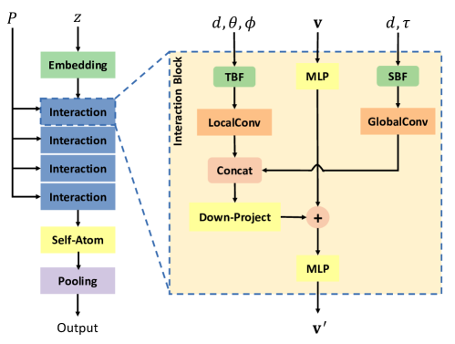
Figure 3: Illustration of ComENet with an overview (left) and the interaction layer (right). TBF and SBF denote the basis functions for tuples $(d,\theta,\phi)$ and $(d,\tau)$. LocalConv and GlobalConv denote the proposed local and global convolution layers. Concat is the concatenation operation and Down-Project is a linear layer to reduce feature dimensions. + denotes the element-wise sum operation.

Based upon the message passing scheme introduced in Sec. 2.5, we propose the complete and efficient graph neural network (ComENet) as shown in Fig. 3. Existing invariant 3D GNN methods [44, 22, 32, 36, 23, 46] share the similar architecture pipeline, which contains an input block, several interaction blocks, and an output block. Our ComENet also follows such architecture fashion along with several novel components, such as self-atom layers and specifically designed local and global graph convolution layers, to better fulfill our proposed message passing scheme in Eq. 1. Generally, ComENet consists of an embedding layer, multiple interaction layers, a self-atom layer, and a pooling layer. To be in line with the message passing scheme in Sec. 2.5, we take the updating process for node $i$’s feature vector $\textbf{v}_{i}$ as an example to describe the network. In practice, feature vectors for all the nodes in a graph are updated simultaneously. In particular, we omit all indices in Fig. 3 and below for clear presentation. Specifically, embedding Layer converts atom type z to an initial node feature vector v via learnable atom type embeddings [45, 22]. Interaction Layer updates node feature vector v based on features of the neighboring nodes and geometric features $(d,\theta,\phi,\tau)$ in Eq. 1 using the local and global graph convolution layers. A detailed description of interaction layer is provided in Appendix A.4. Self-atom layer is used to update each node feature and project the feature dimension into 1. And pooling layer is a sum-pooling performing on all node features to obtain final predictions.

5 Related Work

We consider how to represent 3D information in 3D molecular graphs [3, 10]. One category of methods are equivariant 3D GNNs that directly use coordinates in the CSC as inputs to networks [51, 2, 18, 46, 8]. These methods are efficient but suffer from several setbacks. Firstly, each network component needs to be carefully designed to be rotation equivariant of input graphs. Secondly, the reason why this category of methods are efficient lies in that they only use the type-1 basis in Spherical harmonics, which is an approximation essentially. It is proved in  [51] that theoretically, $l$ is infinite in terms of type-$l$ basis. In practice, $l$ should be at least 2 for achieving satisfactory performance. Type-1 basis essentially coerces the conv kernel to be in a narrow learning space, which imposes a hard constraint on the network capability. However, when using type-2 basis, the conv kernel can be more expressive while the efficiency issue would emerge as a new bottleneck. Thirdly, the performance of such equivariant GNNs is shown to be worse than invariant 3D GNNs [36].

In this work, we follow invariant 3D GNNs to inherit the merit of SE(3)-invariance by investigating relative 3D information, which is used in both representation learning tasks  [45, 22, 32, 47, 36, 23] and coordinates generation tasks [19, 48, 49, 58, 30, 6]. Since the relative information is SE(3)-invariant of input 3D graphs, the employed networks favorably achieve the invariance merit. We focus on the 3D graph learning problem and existing methods either capture partial 3D information or suffer from high computational cost. For example, SchNet [45] only considers distance information and DimeNet [22] further incorporates angles between bonds. They both integrate incomplete 3D information that the network capacity is limited in practice. SphereNet [36] generates approximate complete 3D representations by using distance, angle, and torsion information but the complexity is $O(nk^{2})$. GemNet [23] is based on quadruplets of nodes, which is more expensive. Our objective is to build a fully complete 3D graph net with a much lower computational budget.

There also exist some methods in literature using both absolute and relative 3D information [25, 28, 60]. In this work, we only use relative information as input to avoid inherent limitations of equivariant 3D GNNs. Moreover, we design a novel message passing such that the computational cost is comparable with that of equivariant 3D GNNs.

Table 1: Statistics of the datasets.

Dataset	OC20	Molecule3D	QM9
# Graphs	660,010	3,899,647	130,831
Split Type	Pre-defined	Random/Scaffold	Random
Split Ratio	70:15:15	6:2:2	84:8:8
# Nodes/Graph	77.75	29.11	18.02

6 Experiments

We examine the power and efficiency of ComENet on two large-sacle datasets including Open Catalyst 2020 (OC20) [12] and Molecule3D [58], and the mostly commonly used datastet QM9 [42]. The statistics of three datasets are provided in Table 1. Detailed descriptions of the datasets are provided in Appendix A.5. In particular, the Molecule3D contains about 4 million 3D molecular graphs, and the OC20 has the average graph size of 77.75. Baseline methods include GIN-Virtual [27], CGCNN [56], SchNet [45], PhysNet [52], MGCN [37], DimeNet [22], DimeNet++ [32], SphereNet [36], PaiNN [46], GemNet [23]. Unless otherwise specified, the values for baseline methods are taken from the referred papers. For the ComENet, we use data loader in the PyTorch Geometric library [15] to load the datasets. All the models are trained using the Adam optimizer [31] and the optimal hyperparameters are obtained on validation sets using grid search. Experimental setup and search space for all models are provided in Appendix A.6. Code is integrated in the DIG library [34] and available at https://github.com/divelab/DIG.

Table 2: Results on IS2RE including computing cost in training&inference and performance in terms of energy MAE and the percentage of EwT of the ground truth energy. Training time is the average time per epoch during training using 1 GPU. Performance is reported for models trained on the All training dataset. The best performance is shown in bold and the second best is shown with underlines.

	Time		Energy MAE [eV] $\downarrow$					EwT $\uparrow$
Model	Train	Infer.	ID	OOD Ads	OOD Cat	OOD Both	Average	ID	OOD Ads	OOD Cat	OOD Both	Average
CGCNN	18min	1min	0.6203	0.7426	0.6001	0.6708	0.6585	3.36%	2.11%	3.53%	2.29%	2.82%
SchNet	10min	1min	0.6465	0.7074	0.6475	0.6626	0.6660	2.96%	2.22%	3.03%	2.38%	2.65%
DimeNet++	230min	4min	0.5636	0.7127	0.5612	0.6492	0.6217	4.25%	2.48%	4.40%	2.56%	3.42%
GemNet-T	200min	4min	0.5561	0.7342	0.5659	0.6964	0.6382	4.51%	2.24%	4.37%	2.38%	3.38%
SphereNet	290min	5min	0.5632	0.6682	0.5590	0.6190	0.6023	4.56%	2.70%	4.59%	2.70%	3.64%
ComENet	20min	1min	0.5558	0.6602	0.5491	0.5901	0.5888	4.17%	2.71%	4.53%	2.83%	3.56%

6.1 OC20

The Open Catalyst 2020 (OC20) dataset is a newly released large-scale dataset with millions of DFT relaxations to model and discover catalysts. In this work, we focus on Initial Structure to Relaxed Energy (IS2RE) task, which is the most common task in catalyst discovery. Descriptions of the data and tasks are provided in Appendix A.5. The ground truth of the test set is not publicly available, therefore, we compare the results of different methods on the validation set. The evaluation metrics include the energy MAE and the percentage of Energies within a Threshold (EwT) of the ground truth energy. The values for the baseline methods are taken from Chanussot et al. [11], Liu et al. [36]. Notably, we aim to predict relaxed energy directly from initial structure and do not compare with some methods using relaxation [12], trajectory information, or relaxed structures. Using relaxation [12, 23, 47] is computationally expensive during prediction while the relaxation trajectory and relaxed structures [25, 60] are hard to obtain in practice.

Table 2 shows that ComENet outperforms all the baseline methods in terms of energy MAE, which is also used as the main evaluation metric in the Open Catalyst Challenge [13]. ComENet achieves best performance on two splits and the second best on the other two splits in terms of EwT. Specifically, ComENet reduces the average energy MAE by 0.0135, which is 2.2% of the second best model. Note that ComENet achieves the best results on the OOD Both split in terms of both energy MAE and EwT. In practice, it is common that test data is in the different domain with the training data. Hence, OOD Both can test the generalization capability of learning models. More importantly, ComENet is much more efficient than methods like DimeNet++ and SphereNet. For example, SphereNet needs 5 hours per epoch while ComENet only requires 20 minutes using the same computing infrastructure (NVIDIA RTX A6000 48GB). Overall, compared with existing best methods, ComENet achieves better performance and largely reduces training by at least 10 times.

Table 3: Comparisons between ComENet and other models in terms of computing cost and HOMO-LUMO gap MAE on Molecule3D for both random and scaffold splits. Train time is the average training time per epoch.

	Time		MAE
Model	Train	Inference	Random	Scaffold
GIN-Virtual	15min	2min	0.1036	0.2371
SchNet	14min	3min	0.0428	0.1511
DimeNet++	133min	16min	0.0306	0.1214
SphereNet	182min	28min	0.0301	0.1182
ComENet	22min	3min	0.0326	0.1273

6.2 Molecule3D

The Molecule3D dataset [58] is a newly proposed large-scale dataset, including around 4 million molecules with precise ground-state 3D information derived from DFT and molecular properties. We focus on the prediction of the HOMO-LUMO gap as it is one of the most practically-relevant quantum chemical properties of molecules. A detailed description of the Molecule3D dataset is provided in Appendix A.5. As this is a newly proposed dataset, we run baseline methods including GIN-Virtual [27], SchNet [45], DimeNet++[32] and SphereNet [36], among which GIN-Virtual is a powerful baseline for 2D graphs while the others are for 3D graphs. All the models are trained using the same computing infrastructure (Nvidia GeForce RTX 2080 Ti 11GB).

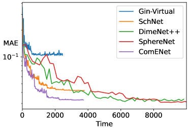
Figure 4: Total training time for different methods on Molecule3D.

Table 3 shows that ComENet dramatically reduces training time by 6-9 times compared with DimeNet++ and SphereNet, and costs similar time as GIN-virtual and SchNet that only considers distance information. In terms of performance, our ComENet performs much better than SchNet for both random and scaffold splits with similar time and computing costs, but a little worse than DimeNet++ and SphereNet. This may be due to the molecules are relatively small in Molecule3D compared with OC20, the structures that our complete strategy can distinguish may not exist in the dataset. However, considering the comparable performance and high efficiency, our ComENet is more practically useful than other methods on such large datasets. In addition, Fig. 4 also shows ComENet either converges much faster in terms of total training time or performs much better compared with other baselines.

6.3 QM9

Table 4: Comparisons between ComENet and other models in terms of MAE and the overall mean std. MAE on QM9.

Property	Unit	SchNet	PhysNet	MGCN	DimeNet	DimeNet++	PaiNN	SphereNet	ComENet
$\mu$	D	0.033	0.0529	0.0560	0.0286	0.0297	0.012	0.0245	0.0245
$\alpha$	${a_{0}}^{3}$	0.235	0.0615	0.0300	0.0469	0.0435	0.045	0.0449	0.0452
$\epsilon_{\text{HOMO}}$	meV	41	32.9	42.1	27.8	24.6	27.6	22.8	23.1
$\epsilon_{\text{LUMO}}$	meV	34	24.7	57.4	19.7	19.5	20.4	18.9	19.8
$\Delta\epsilon$	meV	63	42.5	64.2	34.8	32.6	45.7	31.1	32.4
$\left<R^{2}\right>$	${a_{0}}^{2}$	0.073	0.765	0.110	0.331	0.331	0.066	0.268	0.259
ZPVE	meV	1.7	1.39	1.12	1.29	1.21	1.28	1.12	1.20
$U_{0}$	meV	14	8.15	12.9	8.02	6.32	5.85	6.26	6.59
$U$	meV	19	8.34	14.4	7.89	6.28	5.83	6.36	6.82
$H$	meV	14	8.42	14.6	8.11	6.53	5.98	6.33	6.86
$G$	meV	14	9.4	16.2	8.98	7.56	7.35	7.78	7.98
$c_{\text{v}}$	$\frac{\mbox{cal}}{\mbox{mol K}}$	0.033	0.028	0.038	0.025	0.023	0.024	0.022	0.024
std. MAE	%	1.76	1.37	1.86	1.05	0.98	1.01	0.91	0.93

The QM9 dataset is a widely used dataset for predicting various properties of molecules. The evaluation metrics include the MAE for each property and the overall mean standardized MAE (std. MAE) for all the 12 properties. A detailed description of the dataset is provided in Appendix A.5. Notably, we do not list results for PPGN [38] and Cormorant [2] since they use different train/val/test sizes. Table 4 shows that ComENet is much better than the methods operating in 1-hop neighborhood like SchNet, PhyNet, and MGCN. Compared with DimeNet, DimeNet++, PaiNN, and SphereNet, ComENet achieves similar results on all properties and the overall std. MAE. Consistently, compared with methods operating in 2-hop neighborhood like DimeNet, DimeNet++, and SphereNet, ComENet is much more efficient.

6.4 Ablation Study for Identifying Conformers

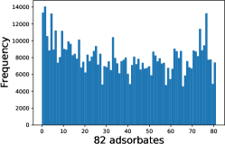
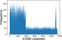
Figure 5: Distributions of adsorbates and catalysts in OC20. For y-axis, frequency counts the number of conformers for each individual adsorbate and catalyst.

As mentioned in Sec. 2.3, rotation angles are the main difference between different conformers [19, 29]. We investigate the contribution of our proposed rotation angles $\tau$ to demonstrate the effectiveness of our global complete representations. We conduct experiments on the OC20 dataset since there exist different conformers for molecules in this dataset. Specifically, there are 660,010 data samples in the OC20 dataset (IS2RE), where each sample is a combination of two parts, namely, adsorbate and catalyst. There are 82 adsorbates and 11,500 catalysts used in the datasets. Each adsorbate inevitably corresponds to different conformers in the dataset, and it is similar to catalyst. We show the number of conformers for each adsorbate and each catalyst in Fig. 5. We remove the rotation angle $\tau$ from ComENet and denote it as "ComENet w/o $\tau$". The results in Table 5 show that removing rotation angles $\tau$ can harm the performance of ComENet, demonstrating the effectiveness of our global complete representations for identifying conformers.

Table 5: Comparisons between ComENet and the model without rotation angles $\tau$ on OC20.

	Energy MAE [eV] $\downarrow$					EwT $\uparrow$
Model	ID	OOD Ads	OOD Cat	OOD Both	Average	ID	OOD Ads	OOD Cat	OOD Both	Average
ComENet	0.5558	0.6602	0.5491	0.5901	0.5888	4.17%	2.71%	4.53%	2.83%	3.56%
ComENet w/o $\tau$	0.5585	0.6851	0.5574	0.6186	0.6049	4.13%	2.65%	4.13%	2.75%	3.42%

7 Conclusions, Limitations, Outlook, and Societal Impacts

3D information is crucial for 3D molecular graph learning. Existing methods either learn partial 3D information or induce high time complexity. We propose ComENet that is both complete in incorporating 3D information and efficient with time complexity of $O(nk)$. Particularly, we propose the novel rotation angles to fulfill global completeness. ComENet can generalize to large-scale datasets, accelerating training and inference by 6-10 times with superior or comparable performance. Even though ComENet is the first complete and the most efficient 3D GNN model, there exists one major limitation, which is not only for ComENet but also for existing 3D GNNs. Basically, existing 3D GNN models are centered on the fact that 3D information is given in data. However, acquiring 3D information itself is difficult and expensive in practice. Current methods rely on experiments or DFT-based computing, which is extremely time-consuming. It would be significant that machine learning models can be developed to tackle this problem. Looking forward, we can derive two directions for fulfilling such objective. Firstly, we can study to generate 3D graphs either from 2D graphs or from scratch by developing generative models, such as VAE, flow and diffusion models. Especially, in some real-world applications like drug discovery, 2D molecules are usually not given. This raises the need of developing new generation methods from scratch. Secondly, we can target at a research case where we have a minimal set of training data with 3D information, but the vast unseen data or new data lack such 3D information. We may develop novel contrastive learning components to force correspondence and consistency between 2D graphs and their 3D geometric views, then integrate such components into end-to-end learning systems for application based on 2D graph data. ComENet can facilitate a plethora of important real-world applications, such as drug discovery and material discovery. It can be used in several research domains including quantum chemistry and physics, material sciences, molecular dynamics simulations, etc. Any negative societal impact associated with those applications and domains can be applied to our method.

Appendix A Appendix

A.1 Algorithm for the Proposed Message Passing

Algorithm 1 The Proposed Message Passing

1:  for $i=1,...,n$ do

2:     for $j=1,...,k$ do

3:        Compute $d_{ij}=||\mathrm{\textbf{p}}_{i}-\mathrm{\textbf{p}}_{j}||_{2}$

4:     end for

5:     Get reference nodes via

$$f_{i}=\mathrm{argmin}_{k\in\mathcal{N}_{i}}(d_{ik}),s_{i}=\mathrm{argmin}_{k\in\mathcal{N}_{i}\backslash\{f_{i}\}}(d_{ik})$$

6:  end for

7:  for $i=1,...,n$ do

8:     for $j=1,...,k$ do

9:        Get reference nodes via

$$f_{i\backslash j}=\begin{cases}f_{i},&\text{if }f_{i}\neq j\\ s_{i},&\text{otherwise}\end{cases},f_{j\backslash i}=\begin{cases}f_{j},&\text{if }f_{j}\neq i\\ s_{j},&\text{otherwise}\end{cases}$$

10:        Compute angles via

$$\theta_{ij} =\mathrm{angle}_{1}(f_{i},i,j),$$

$$\phi_{ij} =\mathrm{angle}_{2}(\mathrm{plane}_{f_{i},i,s_{i}},\mathrm{plane}_{f_{i},i,j}),$$

$$\tau_{ij} =\mathrm{angle}_{3}(\mathrm{plane}_{f_{i\backslash j},i,j},\mathrm{plane}_{i,j,f_{j\backslash i}}),$$

11:     end for

12:     Update node features via Eq. 1

13:  end for

As rigorously shown in Algorithm 1 , there are two nested loops in the message passing. For each nested loop, the complexity for the outer loop is $O(n)$, and the complexity for the inner loop is $O(k)$. Particularly, within the inner loop, the operations are picking proper reference nodes, thus the complexity is simply $O(1)$. Overall, the total complexity of our message passing is $O(nk)$. Importantly, the efficiency of our method is also demonstrated in Sec. 6 that ComeNet is 6-10 times faster than SphereNet. Actually, the training time of ComENet is similar to SchNet whose complexity is also $O(nk)$.

A.2 SE(3)

SE(3) is the Special Euclidean group in 3 dimensions, including all rotations and translations in 3D. It is the set of $4\times 4$ real matrices of the form

$$\begin{bmatrix}Rot&\textbf{t}\\ 0&1\end{bmatrix}=\begin{bmatrix}r_{11}&r_{12}&r_{13}&t_{1}\\ r_{21}&r_{22}&r_{23}&t_{2}\\ r_{31}&r_{32}&r_{33}&t_{3}\\ 0&0&0&1\end{bmatrix},$$ (2)

where $Rot\in\mathrm{SO(3)}$ and $\textbf{t}\in\mathbb{R}^{3}$. The SO(3) is the set of $3\times 3$ real matrices $Rot$ satisfying $Rot^{T}Rot=I$ and $\det(Rot)=1$.

A.3 Proofs of Lemma 1

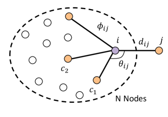
(a) Case (1): $i$ has more than one neighboring nodes $c_{1,2,...}$

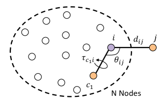
(b) Case (2): $i$ only has one neighboring node $c_{1}$

Figure 6: Two cases for proving Lemma 1 when generalizing the size of a 3D graph from $k$ to $k+1$.

Proof.

We employ contradiction to prove it. Basically, there exist two cases when adding this new node $j$, as illustrated in Fig. 6 and described as following. Case (1): $i$ has more than one neighboring nodes $c_{1,2,...}$; Case (2): $i$ only has one neighboring node $c_{1}$.

Generally, in case (1), we need to prove $\textbf{p}_{ij}$ is uniquely defined as $(d_{ij},\theta_{ij},\phi_{ij})$; in case (2), we need to prove $\textbf{p}_{ij}$ is uniquely defined as $(d_{ij},\theta_{ij},\tau_{c_{1}i})$. We assume there exists another location for $j$ such that there is a different relative location vector $\widetilde{\textbf{p}}_{ij}$, and this assumption leads to contradiction. The proofs of both cases are provided below. ∎

Proof of case (1): In case (1), we need to prove $\textbf{p}_{ij}$ is uniquely defined as $(d_{ij},\theta_{ij},\phi_{ij})$. Based on the notations defined in Sec. 2.4, we have

$$\left<\textbf{p}_{ij},\textbf{p}_{ij}\right>=d^{2}_{ij},$$ (3)

$$\left<\textbf{p}_{if_{i}},\textbf{p}_{ij}\right>=d_{if_{i}}d_{ij}cos\theta_{ij},$$

$$\left<T(\textbf{p}_{is_{i}}),T(\textbf{p}_{ij})\right>=\|T(\textbf{p}_{is_{i}})\|\|T(\textbf{p}_{ij})\|cos\phi_{ij},$$

$$\left<T(\textbf{p}_{is_{i}})\times T(\textbf{p}_{ij}),\textbf{p}_{if_{i}}\right>=d_{if_{i}}\|T(\textbf{p}_{is_{i}})\|\|T(\textbf{p}_{ij})\|sin\phi_{ij},$$

where $T$ denotes an operator of projection to the plane perpendicular to $\textbf{p}_{if_{i}}$. Apparently, all the quantities on the right side are known based on Sec. 2.4. Assume the solution set contains at least two different solutions $\textbf{p}_{ij}$ and $\widetilde{\textbf{p}}_{ij}$. Eq. LABEL:eq:case1_1 can simply imply that

$$\left<\textbf{p}_{if_{i}},\textbf{p}_{ij}-\widetilde{\textbf{p}}_{ij}\right>=0,$$ (4)

$$\left<T(\textbf{p}_{is_{i}}),\textbf{p}_{ij}-\widetilde{\textbf{p}}_{ij}\right>=0,$$

$$\left<T(\textbf{p}_{is_{i}})\times(\textbf{p}_{ij}-\widetilde{\textbf{p}}_{ij}),\textbf{p}_{if_{i}}\right>=0.$$

Apparently, both $T(\textbf{p}_{is_{i}})$ and $\textbf{p}_{ij}-\widetilde{\textbf{p}}_{ij}$ are in the plane perpendicular to $\textbf{p}_{if_{i}}$. Hence, $T(\textbf{p}_{is_{i}})\times(\textbf{p}_{ij}-\widetilde{\textbf{p}}_{ij})=\alpha\textbf{p}_{if_{i}}$ holds for some $\alpha\neq 0$. However, from Eq. LABEL:eq:case1_2, we have

$$\left<T(\textbf{p}_{is_{i}})\times(\textbf{p}_{ij}-\widetilde{\textbf{p}}_{ij}),\textbf{p}_{if_{i}}\right>=\alpha\left<\textbf{p}_{if_{i}},\textbf{p}_{if_{i}}\right>=0.$$ (5)

Since $\alpha\neq 0$ and $\textbf{p}_{if_{i}}\neq\textbf{0}$, Eq. LABEL:eq:case1_3 causes a contradiction. Thus, the solution set contains a unique solution.

Proof of case (2): In case (2), we need to prove $\textbf{p}_{ij}$ is uniquely defined by $(d_{ij},\theta_{ij},\tau_{c_{1}i})$. Based on the notations defined in Sec. 2.4 and Sec. 2.2, we have

$$\left<\textbf{p}_{ij},\textbf{p}_{ij}\right>=d^{2}_{ij},$$ (6)

$$\left<\textbf{p}_{if_{i}},\textbf{p}_{ij}\right>=d_{if_{i}}d_{ij}cos\theta_{ij},$$

$$\left<T(\textbf{p}_{f_{i}f_{f_{i}\backslash i}}),T(\textbf{p}_{ij})\right>=\|T(\textbf{p}_{f_{i}f_{f_{i}\backslash i}})\|\|T(\textbf{p}_{ij})\|cos\tau_{c_{1}i},$$

$$\left<T(\textbf{p}_{f_{i}f_{f_{i}\backslash i}})\times T(\textbf{p}_{ij}),\textbf{p}_{if_{i}}\right>=d_{if_{i}}\|T(\textbf{p}_{f_{i}f_{f_{i}\backslash i}})\|\|T(\textbf{p}_{ij})\|sin\tau_{c_{1}i},$$

where $T$ still denotes an operator of projection to the plane perpendicular to $\textbf{p}_{if_{i}}$. Similarly, all the quantities on the right side are known based on Sec. 2.4 and Sec. 2.2. Assume the solution set contains at least two different solutions $\textbf{p}_{ij}$ and $\widetilde{\textbf{p}}_{ij}$. Eq. LABEL:eq:case2_1 can simply imply that

$$\left<\textbf{p}_{if_{i}},\textbf{p}_{ij}-\widetilde{\textbf{p}}_{ij}\right>=0,$$ (7)

$$\left<T(\textbf{p}_{f_{i}f_{f_{i}\backslash i}}),\textbf{p}_{ij}-\widetilde{\textbf{p}}_{ij}\right>=0,$$

$$\left<T(\textbf{p}_{f_{i}f_{f_{i}\backslash i}})\times(\textbf{p}_{ij}-\widetilde{\textbf{p}}_{ij}),\textbf{p}_{if_{i}}\right>=0.$$

Both $T(\textbf{p}_{f_{i}f_{f_{i}\backslash i}})$ and $\textbf{p}_{ij}-\widetilde{\textbf{p}}_{ij}$ are in the plane perpendicular to $\textbf{p}_{if_{i}}$. Hence, $T(\textbf{p}_{f_{i}f_{f_{i}\backslash i}})\times(\textbf{p}_{ij}-\widetilde{\textbf{p}}_{ij})=\alpha\textbf{p}_{if_{i}}$ holds for some $\alpha\neq 0$. However, from Eq. LABEL:eq:case2_2, we have

$$\left<T(\textbf{p}_{f_{i}f_{f_{i}\backslash i}})\times(\textbf{p}_{ij}-\widetilde{\textbf{p}}_{ij}),\textbf{p}_{if_{i}}\right>=\alpha\left<\textbf{p}_{if_{i}},\textbf{p}_{if_{i}}\right>=0.$$ (8)

Since $\alpha\neq 0$ and $\textbf{p}_{if_{i}}\neq\textbf{0}$, Eq. LABEL:eq:case2_3 causes a contradiction. Thus, the solution set contains a unique solution.

A.4 Model architecture

Interaction Layer updates each node feature vector v based on features of the neighboring nodes and the corresponding 3D information in $P$. Firstly, it converts 3D information in $P$ to a set of geometries based on the proposed complete geometric transformation $\mathcal{T}$ and message passing scheme. Since distance is the most important geometry, we also consider $d$ in global representation and split the output of $\mathcal{T}$ into two tuples $(d,\theta,\phi)$ and $(d,\tau)$, for local and global representations, respectively.

Importantly, the tuples $(d,\theta,\phi)$ and $(d,\tau)$ cannot serve as immediate inputs to the network. They need to be transformed into physically meaningful vectors based on quantum-based basis functions. As in previous studies [28, 22, 36, 23], we test different basis functions including MLP, Gaussian and sine functions, spherical Bessel functions, and spherical harmonics. We found spherical Bessel and spherical harmonics perform best. Formally, the basis function for tuple $(d,\theta,\phi)$ is TBF $j_{\ell}\left(\frac{\beta_{\ell n}}{c}d\right)Y_{\ell}^{m}(\theta,\phi)$, where $j_{\ell}(\cdot)$ is a spherical Bessel function of order $\ell$, $Y_{\ell}^{m}$ is a spherical harmonic function of degree $m$ and order $\ell$, $c$ is the cutoff, and $\beta_{\ell n}$ is the $n$-th root of the Bessel function of order $\ell$. The basis function for tuple $(d,\tau)$ is SBF $j_{\ell}\left(\frac{\beta_{\ell n}}{c}d\right)Y_{\ell}^{0}(\tau)$. These two basis functions are also used in SphereNet [36] and GemNet [23].

The two physically meaningful vectors from TBF and SBF are then imported into a local convolution layer and a global convolution layer, respectively. For both convolution layers, we use the GraphConv [40] implemented in the PyTorch Geometric library [15]. The vectors from the basis functions are used as edge weights in the convolution layers. The outputs of local and global convolution layers are concatenated to generate a new node feature vector. Then the concatenated vector is forwarded into several linear layers to generate the updated feature vector $\textbf{v}^{\prime}$.

A.5 Data Description

OC20. The Open Catalyst 2020 (OC20) dataset [12] is a newly released dataset to model and discover catalysts. Specifically, the goal is efficient DFT approximation of structure relaxation, which is a fundamental calculation in catalysis to determine a structure’s activity and selectivity. All the structures in the dataset contain a surface and an adsorbate, and the surface is defined by a unit cell that is periodic in all directions. There are three tasks including Structure to Energy and Forces (S2EF), Initial Structure to Relaxed Structure (IS2RS), and Initial Structure to Relaxed Energy (IS2RE).

In this work, we focus on Initial Structure to Relaxed Energy (IS2RE) task, which is the most common task in catalysis as the relaxed energies are often correlated with catalyst activity and selectivity. The dataset for IS2RE is originally split into training, validation, and test sets. The training set contains 460,328 structures and the validation set has four splits including in-domain (ID), out-of-domain adsorbate (OOD Ads), out-of-domain catalyst (OOD Cat), and out-of-domain adsorbate and catalyst (OOD Both), with 24,733, 24,961, 24,738, 24,971 structures respectively.

Molecule3D. The Molecule3D dataset [58] is a newly proposed large-scale dataset, including around 4 million molecules with precise ground-state geometries derived from DFT. The dataset is collected from PubChemQC [41] and designed for predicting 3D geometries from molecular graphs [58] while we aim to learn representations and predict properties for molecules based on their geometries. The dataset contains 3,899,647 molecules and is split into training, validation, and test sets via random and scaffold split with ratio 6:2:2. Random split ensures the training, validation, and test data are sampled from the same distribution while scaffold split leads to a distribution shift between training and test data. The evaluation metric is the MAE between the predictions and the ground truth.

QM9. The QM9 dataset [42] is a widely used dataset for predicting various properties of molecules. It includes geometric, energetic, electronic, and thermodynamic properties for 134k stable small organic molecules. The dataset is split into three sets, where the training set contains 110,000, the validation set contains 10,000, and the test set contains 10,831 molecules. The twelve properties are dipole moment ($\mu$), isotropic polarizability ($\alpha$), highest occupied molecular orbital energy ($\epsilon_{\text{HOMO}}$), lowest unoccupied molecular orbital energy ($\epsilon_{\text{LUMO}}$), gap between $\epsilon_{\text{HOMO}}$ and $\epsilon_{\text{LUMO}}$, electronic spatial extent ($\left<R^{2}\right>$), zero point vibrational energy (ZPVE), internal energy at 0K ($U_{0}$), internal energy at 298.15K ($U$) , enthalpy at 298.15K ($H$), free energy at 298.15K ($G$) , and heat capavity at 298.15K ($c_{\text{v}}$).

A.6 Experimental Setup

ComENet. The values/search space of model and training hyperparameters for ComENet on OC20, Molecule3D, and QM9 are provided in Table 6 and Table 7. For Molecule3D and QM9, the optimal hyperparameters are chosen by the performance on the validation sets. For OC20, since the final comparison results are on validation set, we firstly use 10% of the training data to choose optimal hyperparameters, then train our model on whole training data. Specifically, we use a larger cutoff value for OC20 to generate graphs and larger hidden dimensions for OC20 and Molecule3D. All models are trained on NVIDIA GeForce RTX 2080 Ti 11GB GPU for Molecule3D and QM9. For the OC20 dataset, we use NVIDIA RTX A6000 48GB GPU. Note that one experiment is only conducted on one GPU.

Baselines for Molecule3D. As Molecule3D is a newly proposed dataset, we run experiments and provide results for baseline methods including GIN-Virtual [27], SchNet [45], DimeNet++[32] and SphereNet [36]. All the models are trained on one GPU (Nvidia GeForce RTX 2080 Ti 11GB). The model hyperparameters and training hyperparameters are listed in Table 8 and Table 9. The optimal hyperparameters are chosen by the performance on validation set. Note that for DimeNet++[32] and SphereNet [36], the maximum batch size is 32 due to the GPU memory limitation.

Table 6: Model hyperparameters for ComENet.

	Values/ search space
Model Hyperparameters	OC20	Molecule3D	QM9
Number of layers	4, 5, 6	4, 5, 6, 8	4, 5, 6
Cutoff	6.0, 8.0	5.0	5.0
Hidden dim	128, 256, 512	128, 256, 512	128, 256
Hidden dim in Self-Atom layer	128, 256, 512	128, 256, 512	128, 256
Number of layers in Self-Atom layer	2, 3, 4	2, 3, 4	2, 3, 4
Number of layers of the MLP in Interaction layer	2, 3, 4	2, 3, 4	2, 3, 4
Distance embedding dim	6, 12	6, 12	6, 12
Angle embedding dim	3, 6	3, 6	3, 6

Table 7: Training hyperparameters for ComENet.

	Values/ search space
Training hyperparameters	OC20	Molecule3D	QM9
Epochs	20	300	1000
Batch size	64, 128	128, 256	32, 64, 128
Learning rate 1e-3, 5e-4, 2e-4	1e-3, 5e-4, 2e-4	1e-3, 5e-4, 2e-4	1e-3, 5e-4, 2e-4
Learning rate decay factor	0.4, 0.5, 0.6	0.4, 0.5, 0.6	0.4, 0.5, 0.6
Learning rate decay epochs	Milestone [4,7,10,12]	20, 30, 50	100, 200
Warmup epochs	2	–	–
Warmup factor	0.2	–	–

Table 8: Model hyperparameters for baseline methods on Molecule3D.

	Values/ search space
Model Hyperparameters	GIN-Virtual	SchNet	DimeNet++	SphereNet
Number of layers	4, 6, 8	4, 6, 8	3, 4, 5, 6	3, 4, 5, 6
Cutoff	-	10.0	6.0	6.0
Hidden dim	600	256	128	128

Table 9: Training hyperparameters for baseline methods on Molecule3D.

	Values/ search space
Training hyperparameters	GIN-Virtual	SchNet	DimeNet++	SphereNet
Epochs	300	300	300	300
Batch size	64, 128, 256	64, 128, 256	16, 32	16, 32
Learning rate	1e-3, 5e-4, 2e-4	1e-3, 5e-4, 2e-4	1e-3, 5e-4, 2e-4	1e-3, 5e-4, 2e-4
Learning rate decay factor	0.4, 0.5, 0.6	0.4, 0.5, 0.6	0.4, 0.5, 0.6	0.4, 0.5, 0.6
Learning rate decay epochs	20, 30, 50	20, 30, 50	20, 30, 50	20, 30, 50

References

- Adams et al. [2022] Keir Adams, Lagnajit Pattanaik, and Connor W. Coley. Learning 3D representations of molecular chirality with invariance to bond rotations. In International Conference on Learning Representations, 2022. URL https://openreview.net/forum?id=hm2tNDdgaFK.
- Anderson et al. [2019] Brandon Anderson, Truong-Son Hy, and Risi Kondor. Cormorant: Covariant molecular neural networks. In Proceedings of the 33st International Conference on Neural Information Processing Systems, pages 14537–14546, 2019.
- Atz et al. [2021] Kenneth Atz, Francesca Grisoni, and Gisbert Schneider. Geometric deep learning on molecular representations. Nature Machine Intelligence, pages 1–10, 2021.
- Axelrod and Gomez-Bombarelli [2020] Simon Axelrod and Rafael Gomez-Bombarelli. Molecular machine learning with conformer ensembles. arXiv preprint arXiv:2012.08452, 2020.
- Axelrod and Gomez-Bombarelli [2022] Simon Axelrod and Rafael Gomez-Bombarelli. GEOM, energy-annotated molecular conformations for property prediction and molecular generation. Scientific Data, 9(1):1–14, 2022.
- Baek et al. [2021] Minkyung Baek, Frank DiMaio, Ivan Anishchenko, Justas Dauparas, Sergey Ovchinnikov, Gyu Rie Lee, Jue Wang, Qian Cong, Lisa N Kinch, R Dustin Schaeffer, et al. Accurate prediction of protein structures and interactions using a three-track neural network. Science, 373(6557):871–876, 2021.
- Battaglia et al. [2018] Peter W Battaglia, Jessica B Hamrick, Victor Bapst, Alvaro Sanchez-Gonzalez, Vinicius Zambaldi, Mateusz Malinowski, Andrea Tacchetti, David Raposo, Adam Santoro, Ryan Faulkner, et al. Relational inductive biases, deep learning, and graph networks. arXiv preprint arXiv:1806.01261, 2018.
- Batzner et al. [2022] Simon Batzner, Albert Musaelian, Lixin Sun, Mario Geiger, Jonathan P Mailoa, Mordechai Kornbluth, Nicola Molinari, Tess E Smidt, and Boris Kozinsky. E(3)-equivariant graph neural networks for data-efficient and accurate interatomic potentials. Nature communications, 13(1):1–11, 2022.
- Borgwardt et al. [2005] Karsten M Borgwardt, Cheng Soon Ong, Stefan Schönauer, SVN Vishwanathan, Alex J Smola, and Hans-Peter Kriegel. Protein function prediction via graph kernels. Bioinformatics, 21(suppl_1):i47–i56, 2005.
- Bronstein et al. [2021] Michael M Bronstein, Joan Bruna, Taco Cohen, and Petar Veličković. Geometric deep learning: Grids, groups, graphs, geodesics, and gauges. arXiv preprint arXiv:2104.13478, 2021.
- Chanussot et al. [2021a] Lowik Chanussot, Abhishek Das, Siddharth Goyal, Thibaut Lavril, Muhammed Shuaibi, Morgane Riviere, Kevin Tran, Javier Heras-Domingo, Caleb Ho, Weihua Hu, et al. Correction to “the open catalyst 2020 (oc20) dataset and community challenges”. ACS Catalysis, 11(21):13062–13065, 2021a.
- Chanussot et al. [2021b] Lowik Chanussot, Abhishek Das, Siddharth Goyal, Thibaut Lavril, Muhammed Shuaibi, Morgane Riviere, Kevin Tran, Javier Heras-Domingo, Caleb Ho, Weihua Hu, et al. Open catalyst 2020 (OC20) dataset and community challenges. ACS Catalysis, 11(10):6059–6072, 2021b.
- Chanussot et al. [2021c] Lowik Chanussot, Abhishek Das, Siddharth Goyal, Thibaut Lavril, Muhammed Shuaibi, Morgane Riviere, Kevin Tran, et al. Open Catalyst Challenge. https://opencatalystproject.org/challenge.html, 2021c.
- Duvenaud et al. [2015] David K Duvenaud, Dougal Maclaurin, Jorge Iparraguirre, Rafael Bombarell, Timothy Hirzel, Alán Aspuru-Guzik, and Ryan P Adams. Convolutional networks on graphs for learning molecular fingerprints. Advances in Neural Information Processing Systems, 28:2224–2232, 2015.
- Fey and Lenssen [2019] Matthias Fey and Jan E. Lenssen. Fast graph representation learning with PyTorch Geometric. In ICLR Workshop on Representation Learning on Graphs and Manifolds, 2019.
- Fout et al. [2017] Alex Fout, Jonathon Byrd, Basir Shariat, and Asa Ben-Hur. Protein interface prediction using graph convolutional networks. In Proceedings of the 31st International Conference on Neural Information Processing Systems, pages 6533–6542, 2017.
- Fu et al. [2022] Cong Fu, Xuan Zhang, Huixin Zhang, Hongyi Ling, Shenglong Xu, and Shuiwang Ji. Lattice convolutional networks for learning ground states of quantum many-body systems. arXiv preprint arXiv:2206.07370, 2022.
- Fuchs et al. [2020] Fabian Fuchs, Daniel Worrall, Volker Fischer, and Max Welling. SE(3)-Transformers: 3D roto-translation equivariant attention networks. Advances in Neural Information Processing Systems, 33, 2020.
- Ganea et al. [2021] Octavian-Eugen Ganea, Lagnajit Pattanaik, Connor W Coley, Regina Barzilay, Klavs F Jensen, William H Green, and Tommi S Jaakkola. GeoMol: Torsional geometric generation of molecular 3D conformer ensembles. Advances in Neural Information Processing Systems, 2021.
- Gao and Ji [2019] Hongyang Gao and Shuiwang Ji. Graph U-Nets. In International Conference on Machine Learning, pages 2083–2092. PMLR, 2019.
- Gao et al. [2021] Hongyang Gao, Yi Liu, and Shuiwang Ji. Topology-aware graph pooling networks. IEEE Transactions on Pattern Analysis and Machine Intelligence, 43(12):4512–4518, 2021.
- Gasteiger et al. [2020] Johannes Gasteiger, Janek Groß, and Stephan Günnemann. Directional message passing for molecular graphs. In International Conference on Learning Representations, 2020. URL https://openreview.net/forum?id=B1eWbxStPH.
- Gasteiger et al. [2021] Johannes Gasteiger, Florian Becker, and Stephan Günnemann. Gemnet: Universal directional graph neural networks for molecules. Advances in Neural Information Processing Systems, 34:6790–6802, 2021.
- Gilmer et al. [2017] Justin Gilmer, Samuel S Schoenholz, Patrick F Riley, Oriol Vinyals, and George E Dahl. Neural message passing for quantum chemistry. In Proceedings of the 34th International Conference on Machine Learning-Volume 70, pages 1263–1272. JMLR. org, 2017.
- Godwin et al. [2022] Jonathan Godwin, Michael Schaarschmidt, Alexander L Gaunt, Alvaro Sanchez-Gonzalez, Yulia Rubanova, Petar Veličković, James Kirkpatrick, and Peter Battaglia. Simple GNN regularisation for 3D molecular property prediction and beyond. In International Conference on Learning Representations, 2022. URL https://openreview.net/forum?id=1wVvweK3oIb.
- Hoogeboom et al. [2022] Emiel Hoogeboom, Victor Garcia Satorras, Clément Vignac, and Max Welling. Equivariant diffusion for molecule generation in 3D. In International Conference on Machine Learning, pages 8867–8887. PMLR, 2022.
- Hu et al. [2021a] Weihua Hu, Matthias Fey, Hongyu Ren, Maho Nakata, Yuxiao Dong, and Jure Leskovec. OGB-LSC: A large-scale challenge for machine learning on graphs. In Thirty-fifth Conference on Neural Information Processing Systems Datasets and Benchmarks Track (Round 2), 2021a. URL https://openreview.net/forum?id=qkcLxoC52kL.
- Hu et al. [2021b] Weihua Hu, Muhammed Shuaibi, Abhishek Das, Siddharth Goyal, Anuroop Sriram, Jure Leskovec, Devi Parikh, and C Lawrence Zitnick. ForceNet: A graph neural network for large-scale quantum calculations. arXiv preprint arXiv:2103.01436, 2021b.
- Jing et al. [2022] Bowen Jing, Gabriele Corso, Regina Barzilay, and Tommi S. Jaakkola. Torsional diffusion for molecular conformer generation. In ICLR Workshop on Deep Generative Models for Highly Structured Data, 2022. URL https://openreview.net/forum?id=SBgNnnVuwbc.
- Jumper et al. [2021] John Jumper, Richard Evans, Alexander Pritzel, Tim Green, Michael Figurnov, Olaf Ronneberger, Kathryn Tunyasuvunakool, Russ Bates, Augustin Žídek, Anna Potapenko, et al. Highly accurate protein structure prediction with AlphaFold. Nature, 596(7873):583–589, 2021.
- Kingma and Ba [2015] Diederik Kingma and Jimmy Ba. Adam: A method for stochastic optimization. The International Conference on Learning Representations, 2015.
- Klicpera et al. [2020] Johannes Klicpera, Shankari Giri, Johannes T Margraf, and Stephan Günnemann. Fast and uncertainty-aware directional message passing for non-equilibrium molecules. In NeurIPS-W, 2020.
- Kochkov et al. [2021] Dmitrii Kochkov, Tobias Pfaff, Alvaro Sanchez-Gonzalez, Peter Battaglia, and Bryan K Clark. Learning ground states of quantum hamiltonians with graph networks. arXiv preprint arXiv:2110.06390, 2021.
- Liu et al. [2021] Meng Liu, Youzhi Luo, Limei Wang, Yaochen Xie, Hao Yuan, Shurui Gui, Haiyang Yu, Zhao Xu, Jingtun Zhang, Yi Liu, Keqiang Yan, Haoran Liu, Cong Fu, Bora M Oztekin, Xuan Zhang, and Shuiwang Ji. DIG: A turnkey library for diving into graph deep learning research. Journal of Machine Learning Research, 22(240):1–9, 2021. URL http://jmlr.org/papers/v22/21-0343.html.
- Liu et al. [2020] Yi Liu, Hao Yuan, Lei Cai, and Shuiwang Ji. Deep learning of high-order interactions for protein interface prediction. In Proceedings of the 26th ACM SIGKDD International Conference on Knowledge Discovery & Data Mining, pages 679–687, 2020.
- Liu et al. [2022] Yi Liu, Limei Wang, Meng Liu, Yuchao Lin, Xuan Zhang, Bora Oztekin, and Shuiwang Ji. Spherical message passing for 3D molecular graphs. In International Conference on Learning Representations, 2022. URL https://openreview.net/forum?id=givsRXsOt9r.
- Lu et al. [2019] Chengqiang Lu, Qi Liu, Chao Wang, Zhenya Huang, Peize Lin, and Lixin He. Molecular property prediction: A multilevel quantum interactions modeling perspective. In Proceedings of the AAAI Conference on Artificial Intelligence, volume 33, pages 1052–1060, 2019.
- Maron et al. [2019] Haggai Maron, Heli Ben-Hamu, Hadar Serviansky, and Yaron Lipman. Provably powerful graph networks. Advances in Neural Information Processing Systems, 32:2153–2164, 2019.
- Morehead et al. [2022] Alex Morehead, Chen Chen, and Jianlin Cheng. Geometric transformers for protein interface contact prediction. In International Conference on Learning Representations, 2022. URL https://openreview.net/forum?id=CS4463zx6Hi.
- Morris et al. [2019] Christopher Morris, Martin Ritzert, Matthias Fey, William L Hamilton, Jan Eric Lenssen, Gaurav Rattan, and Martin Grohe. Weisfeiler and leman go neural: Higher-order graph neural networks. In Proceedings of the AAAI Conference on Artificial Intelligence, volume 33, pages 4602–4609, 2019.
- Nakata and Shimazaki [2017] Maho Nakata and Tomomi Shimazaki. PubChemQC project: a large-scale first-principles electronic structure database for data-driven chemistry. Journal of chemical information and modeling, 57(6):1300–1308, 2017.
- Ramakrishnan et al. [2014] Raghunathan Ramakrishnan, Pavlo O Dral, Matthias Rupp, and O Anatole Von Lilienfeld. Quantum chemistry structures and properties of 134 kilo molecules. Scientific data, 1(1):1–7, 2014.
- Satorras et al. [2021] Vıctor Garcia Satorras, Emiel Hoogeboom, and Max Welling. E (n) equivariant graph neural networks. In International conference on machine learning, pages 9323–9332. PMLR, 2021.
- Schmidhuber [2015] Jürgen Schmidhuber. Deep learning in neural networks: An overview. Neural Networks, 61:85–117, 2015.
- Schütt et al. [2017] Kristof Schütt, Pieter-Jan Kindermans, Huziel Enoc Sauceda Felix, Stefan Chmiela, Alexandre Tkatchenko, and Klaus-Robert Müller. SchNet: A continuous-filter convolutional neural network for modeling quantum interactions. In Advances in Neural Information Processing Systems, pages 991–1001, 2017.
- Schütt et al. [2021] Kristof Schütt, Oliver Unke, and Michael Gastegger. Equivariant message passing for the prediction of tensorial properties and molecular spectra. In International Conference on Machine Learning, pages 9377–9388. PMLR, 2021.
- Shuaibi et al. [2021] Muhammed Shuaibi, Adeesh Kolluru, Abhishek Das, Aditya Grover, Anuroop Sriram, Zachary Ulissi, and C Lawrence Zitnick. Rotation invariant graph neural networks using spin convolutions. arXiv preprint arXiv:2106.09575, 2021.
- Simm et al. [2020] Gregor N. C. Simm, Robert Pinsler, and José Miguel Hernández-Lobato. Reinforcement learning for molecular design guided by quantum mechanics. In Hal Daumé III and Aarti Singh, editors, Proceedings of the 37th International Conference on Machine Learning, volume 119 of Proceedings of Machine Learning Research, pages 8959–8969. PMLR, 2020. URL http://proceedings.mlr.press/v119/simm20b.html.
- Simm et al. [2021] Gregor N. C. Simm, Robert Pinsler, Gábor Csányi, and José Miguel Hernández-Lobato. Symmetry-aware actor-critic for 3D molecular design. In International Conference on Learning Representations, 2021. URL https://openreview.net/forum?id=jEYKjPE1xYN.
- Stokes et al. [2020] Jonathan M Stokes, Kevin Yang, Kyle Swanson, Wengong Jin, Andres Cubillos-Ruiz, Nina M Donghia, Craig R MacNair, Shawn French, Lindsey A Carfrae, Zohar Bloom-Ackermann, et al. A deep learning approach to antibiotic discovery. Cell, 180(4):688–702, 2020.
- Thomas et al. [2018] Nathaniel Thomas, Tess Smidt, Steven Kearnes, Lusann Yang, Li Li, Kai Kohlhoff, and Patrick Riley. Tensor field networks: Rotation-and translation-equivariant neural networks for 3D point clouds. arXiv preprint arXiv:1802.08219, 2018.
- Unke and Meuwly [2019] Oliver T Unke and Markus Meuwly. PhysNet: A neural network for predicting energies, forces, dipole moments, and partial charges. Journal of chemical theory and computation, 15(6):3678–3693, 2019.
- Vignac et al. [2020] Clement Vignac, Andreas Loukas, and Pascal Frossard. Building powerful and equivariant graph neural networks with structural message-passing. Advances in Neural Information Processing Systems, 33:14143–14155, 2020.
- Wang et al. [2022] Zhengyang Wang, Meng Liu, Youzhi Luo, Zhao Xu, Yaochen Xie, Limei Wang, Lei Cai, Qi Qi, Zhuoning Yuan, Tianbao Yang, et al. Advanced graph and sequence neural networks for molecular property prediction and drug discovery. Bioinformatics, 38(9):2579–2586, 2022.
- Wu et al. [2018] Zhenqin Wu, Bharath Ramsundar, Evan N Feinberg, Joseph Gomes, Caleb Geniesse, Aneesh S Pappu, Karl Leswing, and Vijay Pande. MoleculeNet: a benchmark for molecular machine learning. Chemical science, 9(2):513–530, 2018.
- Xie and Grossman [2018] Tian Xie and Jeffrey C Grossman. Crystal graph convolutional neural networks for an accurate and interpretable prediction of material properties. Physical review letters, 120(14):145301, 2018.
- Xu et al. [2019] Keyulu Xu, Weihua Hu, Jure Leskovec, and Stefanie Jegelka. How powerful are graph neural networks? In International Conference on Learning Representations, 2019.
- Xu et al. [2021] Zhao Xu, Youzhi Luo, Xuan Zhang, Xinyi Xu, Yaochen Xie, Meng Liu, Kaleb Dickerson, Cheng Deng, Maho Nakata, and Shuiwang Ji. Molecule3D: A benchmark for predicting 3D geometries from molecular graphs. arXiv preprint arXiv:2110.01717, 2021.
- Yang et al. [2019] Kevin Yang, Kyle Swanson, Wengong Jin, Connor Coley, Philipp Eiden, Hua Gao, Angel Guzman-Perez, Timothy Hopper, Brian Kelley, Miriam Mathea, et al. Analyzing learned molecular representations for property prediction. Journal of chemical information and modeling, 59(8):3370–3388, 2019.
- Ying et al. [2021] Chengxuan Ying, Tianle Cai, Shengjie Luo, Shuxin Zheng, Guolin Ke, Di He, Yanming Shen, and Tie-Yan Liu. Do transformers really perform badly for graph representation? In Thirty-Fifth Conference on Neural Information Processing Systems, 2021. URL https://openreview.net/forum?id=OeWooOxFwDa.
- Zhang et al. [2018] Muhan Zhang, Zhicheng Cui, Marion Neumann, and Yixin Chen. An end-to-end deep learning architecture for graph classification. In Proceedings of the AAAI Conference on Artificial Intelligence, volume 32, 2018.