Semiparametric Single-Index Estimation for Average Treatment Effects

Abstract

We propose a semiparametric method to estimate the average treatment effect under the assumption of unconfoundedness given observational data. Our estimation method alleviates misspecification issues of the propensity score function by estimating the single-index link function involved through Hermite polynomials. Our approach is computationally tractable and allows for moderately large dimension covariates. We provide the large sample properties of the estimator and show its validity. Also, the average treatment effect estimator achieves the parametric rate and asymptotic normality. Our extensive Monte Carlo study shows that the proposed estimator is valid in finite samples. We also provide an empirical analysis on the effect of maternal smoking on babies’ birth weight and the effect of job training program on future earnings.

Keywords: Average treatment effects; Causal inference; Hermite series expansion; Propensity score.

1 Introduction

The literature on program evaluation has received considerable attention and provided primary tools for empirical studies in social science. One of the measures frequently used for program evaluation is the average treatment effect (ATE). The ATE is often estimated with restrictive parametric conditions on either the propensity score function or the outcome equation. However, when those parametric assumptions are violated, the estimator may suffer from non-negligible finite-sample bias.

In this paper, we develop a semiparametric estimation method for the ATE to alleviate the issue of possible misspecifications. Our semiparametric approach imposes a single-index structure on the propensity score function while allowing for a flexible link function that can be approximated by Hermite polynomials. We estimate the index parameter and the link function simultaneously in the infinitely dimensional function space. Our approach is practically tractable and can be applied to models with a large class of error distributions. We establish the identification of the model under some regularity conditions, which are incorporated in our estimation procedure, and show that the proposed average treatment effect estimator achieves the parametric convergence rate and asymptotic normality. Also, by extending the propensity score residual approach in Lee (2017), we propose an estimator that is valid even when the propensity score approaches zero or one.

There are a variety of approaches for estimating the average treatment effects under the assumption of unconfoundedness (see Abadie and Cattaneo, 2018, for an overview). The doubly robust estimators, including the inverse probability weighting estimator augmented with additional terms (e.g. Robins et al., 1994; Robins and Rotnitzky, 1995) and the regression imputation estimator with the propensity score as an additional regressor (e.g. Robins et al., 1992; Scharfstein et al., 1999), have been widely used due to the robustness against model misspecifications. The estimators are valid as long as the specification of either propensity score function or the outcome equation is correct. For example, Bang and Robins (2005), Robins (2000), and Rotnitzky et al. (2012) combine inverse propensity score weighting and matching method with imputation and projection to estimate the treatment effects, while the efficiency of these estimators depends on the choice of tuning parameters and computational implementation. Tan (2006, 2010) proposes a nonparametric doubly robust estimation approach and show that the estimators are efficient if the parametric propensity score model is correctly specified. However, Kang and Schafer (2007) and Vansteelandt et al. (2012) show the doubly robust estimation approach suffers from non-trivial finite sample bias when one of the two models is misspecified, with the bias being large when both models are misspecified.

In order to address concerns about bias reduction, a fast-growing literature focuses on improving the robustness of doubly robust estimators. Hirano et al. (2003) consider a nonparametric method to estimate the propensity score and treatment effects. However, this approach is not feasible for moderately large dimension covariates. Vermeulen and Vansteelandt (2015, 2016) propose a novel data-driven method to reduce estimation bias under the potential misspecification of both models. Farrell (2015) provides an inference approach on average treatment effects that is robust to model selection errors. Sloczynski and Wooldridge (2018) propose a general approach for the doubly robust estimators of average treatment effects under unconfoundedness. Chernozhukov et al. (2018) provide a general method to estimate unknown functions in the nonparametric influence function and apply it to debias the estimators of average treatment effects that are feasible in high-dimensional datasets.

We contribute to this strand of literature by proposing a new average treatment effect estimator that does not rely on either propensity score function or outcome equation specification. Our estimator is computationally simple and easy to implement in empirical studies. The asymptotic variance has a simple explicit form that does not need to be estimated through bootstrapping. The estimator can work well in datasets that are limited overlap in the covariate distributions and is not influenced by the extreme observations in empirical applications. By adopting a flexible assumption on the single index structure of propensity score function, our estimator performs well when there are many covariates compared with nonparametric approaches.

This paper is also related to the literature on the estimation of binary outcome models. Hirano et al. (2003) and Wang et al. (2010) use a nonparametric kernel method to approximate the propensity score function, while the estimation results tend to worsen for many covariates and may not be feasible for moderately large dimension covariates due to the curse of dimensionality. Semiparametric approach with single-index structure can retain flexible specification while avoiding the curse of dimensionality. Sun et al. (2021) propose the semiparametric single-index model for propensity score and use the kernel method to estimate its function form semiparametrically. Liu et al. (2018) relate treatment indicator with the low-dimensional linear structure of the covariates and estimate the propensity score function with a nonparametric link function. Both papers assume the boundedness of the link function and the boundedness of function support, imposing additional constraints on asymptotic theory and numerical performance.

By relaxing the parametric assumption on the propensity score model, we estimate the conditional probability using an orthogonal series-based estimation method. Compared with the approach in Liu et al. (2018) and Sun et al. (2021), our estimation approach requires neither the boundedness of the support of the regression function nor the boundedness of the regression function itself (see Chen, 2007; Dong et al., 2016, 2021; Li and Racine, 2007). It is computationally tractable and allows for moderately large dimension covariates. Our propensity score estimator has a super convergence rate $O_{p}(1/N)$ along the direction of the true parameter and has a standard convergence rate $O_{p}(1/\sqrt{N})$ along with all other directions, where $N$ is the sample size. Our method can be further extended by assuming the conditional probability depends on the covariates vector through several linear combinations (see Koenker and Yoon, 2009; Li et al., 2016; Ma and Zhu, 2012, 2013; Racine and Li, 2004, among others).

The rest of this paper is organized as follows. Section 2 introduces treatment effect parameters of interest and Section 3 explains our semiparametric estimation method. We provide the large sample properties of the estimators in Section 4 and simulation results in Section 5. We present the empirical results regarding the effect of maternal smoking on babies’ birth weight and the effect of job training program on future earnings in Section 6 and conclude in Section 7. Appendix A finally gives the proof of the main theorem of this paper. Due to the space limitation, there are some additional details with results about sieve expansions in Appendix B, detailed proofs in Appendix C, extra simulation results in Appendix D, and extra empirical results in Appendix E.

2 Model and Identification

2.1 Setup

We consider the setup of the binary treatment and adopt the potential outcome framework proposed by Rubin (1974). We use $Y(0)$ and $Y(1)$ to denote the potential outcome without and with the treatment, respectively. Also, $D$ is the treatment indicator taking 1 if an individual receives the treatment and 0 otherwise. For each unit, we observe either $Y(0)$ or $Y(1)$, and the observed outcome is given by:

$$Y:=DY(1)+(1-D)Y(0).$$

Suppose that we observe a vector of covariates $X$ with the support of $\mathcal{X}\subset\mathbb{R}^{d}$ and define the propensity score function $\pi(X):=\Pr(D=1|X)$.

As a measure of treatment effects, we consider the ATE, defined as:

$$\Delta^{ATE}:=\mathbb{E}[Y(1)-Y(0)].$$

Alternatively, Angrist (1998) discusses the variance weighted ATE, defined as:

$$\Delta_{\omega}^{ATE}:=\mathbb{E}\big{[}\omega(X)\mathbb{E}\big{(}Y(1)-Y(0)|X\big{)}\big{]},$$

where $\omega(X):=\operatorname{var}(D|X)/\mathbb{E}[\operatorname{var}(D|X)]$. Because $\operatorname{var}(D|X)=\pi(X)\big{(}1-\pi(X)\big{)}$, the weight $\omega(X)$ assigns higher weights to a subpopulation if its propensity score is closer to $\frac{1}{2}$.

The propensity score function can be used to obtain consistent estimators for the average treatment effect $\Delta^{ATE}$. Rosenbaum and Rubin (1983) show that under the assumption of unconfoundedness given covariates, the confounding bias can be removed using the propensity score function. Hahn (1998) proposes the regression imputation estimator that achieves the semiparametric efficiency bound for estimating average treatment effect $\Delta^{ATE}$. Hirano et al. (2003) show that the inverse probability weighting approach can achieve semiparametric efficiency by estimating propensity score in a nonparametric fashion, while this approach may suffer from the curse of dimensionality in empirical analysis.

2.2 Identification of the Treatment Effect

This subsection introduces assumptions and presents an identification result. The following conditions are introduced.

Assumption 1.

$\big{(}Y(1),Y(0),X,D\big{)}$ have a joint distribution satisfying:

(a)

$\big{(}Y(1),Y(0)\big{)}\ \raisebox{0.50003pt}{\rotatebox[origin={c}]{90.0}{$\models$}}\ D|X$,

(b)

$0<\pi(X)<1$.

1(a), referred as the “unconfoundedness assumption” by Rosenbaum and Rubin (1983), has been widely used in the studies on the treatments effects and program evaluation (e.g., Dehejia and Wahba, 1999; Heckman et al., 1998). The validity of this assumption can be assessed by nonparametric approach (see Rosenbaum, 2002; Ichino et al., 2008, for example). 1(b) ensures that the conditional probability of treatment occurrence for both treated and non-treated units is positive, usually imposed in the inverse propensity weighting approach (Hirano et al., 2003; Firpo, 2007). Rosenbaum and Rubin (1983) refer to the combination of these two assumptions as “strongly ignorable treatment assignment”. Since we can identify the propensity score $\pi(X)$ given the data, we can examine this assumption in practice.

For the estimation of ATE, we consider the following regression model:

$$Y=\big{(}D-\pi(X)\big{)}\beta+U.$$ (1)

We use the following weighted regression model for the weighted ATE:

$$\upsilon(X)^{-1/2}Y=\upsilon(X)^{-1/2}\big{(}D-\pi(X)\big{)}\gamma+U,$$ (2)

where $\upsilon(X):=\pi(X)\{1-\pi(X)\}$ is the variance of the treatment status $D$ conditional on $X$. The weight based on the variance $\upsilon(X)$ assigns a higher weight for a more precise subsample and lower weight to a less precise subsample as the weight function $\upsilon(X)$ associated with the $\Delta_{\omega}^{ATE}$ reaches a maximum at $\pi(X)=0.5$ and declines towards 0 when $\pi(X)$ approaches to 0 or 1. In the equations above, $\beta$ and $\gamma$ are scalar parameters, and $U$ is error term. The lemma below shows that, under 1, the ATE and weighted ATE can be identified from the data; its proof is given in Appendix C.

Lemma 1.

Suppose that 1 holds. Then, we have

1. Parameter $\beta$ in Equation (1) is equivalent to the weighted ATE, or $\beta=\Delta_{\omega}^{ATE}$.

2. Parameter $\gamma$ in Equation (2) is equivalent to the ATE, or $\gamma=\Delta^{ATE}$.

The ATE is derived by taking out the average of individual treatment effects with equal weights, while the weighted ATE assigns higher weights to sub-population that is deemed to be more important and more precise estimators and lower weights to less precise estimators.

3 Estimation

This section proposes the estimator of the treatment effect parameters explained in the previous section. Suppose that we have a sample of size equals to $N$ and observe $\{(Y_{i},X_{i},D_{i})\}_{i=1}^{N}$, which are independent copies of $(Y,X,D)$. From Lemma 1, we can estimate $\Delta^{ATE}$ and $\Delta_{\omega}^{ATE}$, applying a least square estimation for Equations (1) and (2), once the propensity score is obtained. Thus, we shall focus on the estimation of the propensity score. Section 3.1 presents a semiparametric estimation method for the propensity score function and Section 3.2 explains a practical estimation procedure.

3.1 Estimation of the Propensity Score

For the estimation of the propensity score function, we consider a semiparametric approach, in which the propensity function is assumed to have a single-index structure. More specifically, the propensity score is given by

$$\pi(X)=\Lambda\big{(}g_{0}(X^{\prime}\theta_{0})\big{)},$$ (3)

where $\Lambda:\mathbb{R}\to[0,1]$ is a known link function and specified as the logistic function in our analysis i.e., $\Lambda(z)=e^{z}/(1+e^{z})$ for $z\in\mathbb{R}$, $g_{0}:\mathbb{R}\to\mathbb{R}$ is an unknown nonparametric function and $\theta_{0}$ is a $d\times 1$ vector of unknown parameters. The link function $\Lambda(\cdot)$ ensures that the propensity score function is confined to be within the unit interval. We assume that the parameters $\theta_{0}$ is an element of the compact parameter space $\Theta\subset\mathbb{R}^{d}$ and set $\theta_{0}$ to satisfy that $\|\theta_{0}\|=1$ and $\theta_{0,1}>0$ for the purpose of identification. The model permits general forms of heteroskedasticity in the function form of the propensity score. The semiparametric approach with a single-index constraint can retain flexible specifications while avoiding the curse of dimensionality. Our method relies on the optimization with the constraint of the identification condition to derive the estimator of parameter $\theta_{0}$. Compared with the semiparametric approach using nonparametric kernel method (see Liu et al., 2018; Sun et al., 2021), our estimator does not impose restrictions on the link function or its support and establishes the asymptotic theory for inference.

We consider the case where the nonparametric function $g_{0}(\cdot)$ resides in the Hilbert space $\mathcal{L}^{2}$ with a norm $\langle g,h\rangle:=\int g(w)h(w)\exp(-w^{2}/2)dw$ for $g,h\in\mathcal{L}^{2}$. The Hilbert space contains all polynomials, all power functions and all bounded, real-valued functions, which are often encountered in both applications and econometric theory (see Chen, 2007, for a review). Let $\{h_{j}(\cdot)\}_{j=1}^{\infty}$ be the orthonormal basis for the Hilbert space. Then, we have the orthogonal series expansion for any function $g\in\mathcal{L}^{2}$:

$$g(w)=\sum_{j=1}^{\infty}c_{j}h_{j}(w),$$ (4)

where the inner product $c_{j}:=\langle g,h_{j}\rangle$. In practice, one has to choose a truncation parameter $k$ to approximate the infinite series, such that:

$$g(\omega)=\widetilde{g}_{k}(\omega)+\epsilon_{k}(\omega),$$

where $\widetilde{g}_{k}(\omega):=\sum_{j=1}^{k}c_{j}h_{j}(\omega)$ and $\epsilon_{k}(\omega):=\sum_{j=k+1}^{\infty}c_{j}h_{j}(\omega)$.

For the estimation of the single-index model, we consider the maximum likelihood framework and define the log-likelihood function as follows:

$$\ell_{N}\big{(}\theta,\{c_{j}\}_{j=1}^{k}\big{)}:=N^{-1}\sum_{i=1}^{N}\big{[}D_{i}\cdot\ln\Lambda\big{(}\widetilde{g}_{k}(X_{i}^{\prime}\theta)\big{)}+(1-D_{i})\cdot\ln\{1-\Lambda\big{(}\widetilde{g}_{k}(X_{i}^{\prime}\theta)\big{\}}\big{]}.$$

The estimators $\hat{\theta}$ and $\{\hat{c}_{j}\}_{j=1}^{k}$ of $\theta$ and $\{c_{j}\}_{j=1}^{k}$ are defined as the solution to the following maximization problem:

$$\max_{(\theta,\{c_{j}\}_{j=1}^{k})\in\Theta\times\mathbb{R}^{k}}\ell_{N}\big{(}\theta,\{c_{j}\}_{j=1}^{k}\big{)},\ \ \ \mathrm{s.t.}\ \ \|\theta\|=1.$$ (5)

Letting $\widehat{g}_{k}(\cdot):=\sum_{j=1}^{k}\hat{c}_{j}h_{j}(\cdot)$, we have an estimator of the propensity score function:

$$\widehat{\pi}(X):=\Lambda\big{(}\widehat{g}_{k}(X^{\prime}\hat{\theta})\big{)}.$$ (6)

Our estimation approach for the propensity score is based on Dong et al. (2019) that investigate a semi-parametric single-index model where the link function is allowed to be unbounded and has unbounded support. The link function is regarded as a point in an infinitely many dimensional function space and the index parameter and the link function can be estimated simultaneously from an optimization with the constraint of identification condition for the index parameter.

Compared with the least squares approach in Dong et al. (2019), our approach considers the maximum likelihood estimation for propensity score. While we may obtain the estimation results using the delta method based on the least squares approach in Dong et al. (2019), our approach can lead to more efficient estimation for propensity score function.

Our estimator has nice finite sample properties. First, compared with a parametric approach, such as probit and logit, our propensity score estimator is more flexible and less prone to misspecification. Second, the estimator can be used for cases with multiple regressors and avoids the curse of dimensionality commonly encountered in nonparametric methods (e.g., Hahn, 1998; Hirano et al., 2003). Finally, we do not impose any distributional assumptions on the covariates by including continuous, discrete, and categorical variables.

3.2 Estimation Procedure

This subsection provides an estimation procedure for the nonlinear constrained optimization problem in Equation (5) and a procedure for the selection of the truncation parameter $k$ among a set of suitable candidate values.

Given a truncation parameter $k$, we obtain the estimators $\hat{\theta}$ and $\{\hat{c}_{j}\}_{j=1}^{k}$ as follows:

Algorithm 1. For a fixed truncation parameter $k$,

(i) Use a linear regression estimator as the initial estimator $\check{\theta}:=(\sum_{i=1}^{N}X_{i}X_{i}^{\prime})^{-1}\sum_{i=1}^{N}X_{i}D_{i}.$

(ii) Obtain the estimator $\{\hat{c}_{j}\}_{j=1}^{k}$ as the solution to the problem: $\max_{\{c_{j}\}_{j=1}^{k}}\ell_{N}\big{(}\check{\theta},\{c_{j}\}_{j=1}^{k}\big{)}$.

(iii) Given the estimator $\{\hat{c}_{j}\}_{j=1}^{k}$, obtain the estimator $\hat{\theta}$ as the solution to the constrained optimization problem:

$$\max_{\theta,\lambda}\ \ell_{N}\big{(}\theta,\{\hat{c}_{j}\}_{j=1}^{k}\big{)}+\lambda(\|\theta\|^{2}-1),$$

where $\lambda$ is a scalar Lagrange multiplier.

The truncation error becomes negligible asymptotically under the regularity conditions. For the choice of the truncation parameter, we propose the leave-one-out cross-validation as follows:

Algorithm 2. Let $\mathcal{K}$ be a set of candidate values of the truncation parameter.

(i) For each $k\in\mathcal{K}$, we apply Algorithm 1 for the observations $\{(Y_{i},X_{i},D_{i})\}$ without using $j$-th observation and obtain the leave-one-out estimate, denoted by $\widehat{Y}_{k,-j}$.

(ii) The optimal truncation parameter minimizes the prediction mean of squares:

$$\min_{k\in\mathcal{K}}\sum_{j=1}^{N}(\widehat{Y}_{k,-j}-Y_{j})^{2}.$$

4 Asymptotic Properties

To establish asymptotic properties for the average treatment effect estimator, we assume the following conditions and provide justifications for the following assumptions.

Assumption 2.

1. The observations $\{(Y_{i},X_{i},D_{i})\}_{i=1}^{N}$ are independent copies of $(Y,X,D)$.

2. Define the population objective function $\ell(\theta,g):=\mathbb{E}[\ell_{N}(\theta,\{c_{j}\}_{j=1}^{k})]$, where $g(w)=\sum_{j=1}^{\infty}c_{j}h_{j}(w)$. Let $\mathcal{G}$ be a subset of $\mathcal{L}^{2}$ such that $g_{0}\in\mathcal{G}$.

   1. All derivatives $g_{0}^{(j)}(w)\in\mathcal{L}^{2}$ for $j=1,\ldots,r$ and $r\geq 1$.

   2. $\ell(\theta,g)$ has the unique maximum at $(\theta_{0},g_{0})$.

   3. $\sup_{(\theta,g)\in\Theta\times\mathcal{G}}\mathbb{E}\big{\|}\{g^{(1)}(X^{\prime}\theta)\}^{2}XX^{\prime}\big{\|}\leq M$, for some $M>0$.

3. The truncation parameter $k$ satisfies that $k\to\infty$ and $k/\sqrt{N}\rightarrow 0$ as $N\rightarrow\infty$.

2(b) covers assumptions that are commonly used in the existing literature on sieve estimation (see Chen, 2007, for a review) and binary choice model (e.g., Coppejans, 2001; Cosslett, 1983; Ichimura, 1993; Klein and Spady, 1993) as a special case and includes many commonly used distributions such as normal distribution and those possessing compact support. Recall we impose $\|\theta_{0}\|=1$ with $\theta_{0,1}>0$ for identification purpose. The estimator is derived from an optimization with the constraints for index parameter, and we do not need to impose additional parameter normalization conditions. 2(c) imposes the smoothness restrictions on the link function and the divergence restrictions on the truncation parameter to guarantee the truncation error is negligible.

For theoretical developments, we need to assume additional regularity conditions. Since these conditions are standard in the literature, we state the conditions as 3.

Assumption 3.

Let $\zeta$ be a relatively small positive number and $M$, $M_{1}$ and $M_{2}$ be positive constants. Suppose that the following conditions hold:

1. For $\Omega(\zeta)=\big{\{}(\theta,g):\big{\|}(\theta,g)-(\theta_{0},g_{0})\big{\|}_{2}\leq\zeta\big{\}}$,

   $$\sup_{(\theta,g)\in\Omega(\zeta)}\mathbb{E}\big{\|}g^{(2)}(X_{i}^{\prime}\theta)X_{i}X_{i}^{\prime}\big{\|}^{2}\leq M,$$

   $$\sup_{(\theta,g)\in\Omega(\zeta)}\Big{\|}\frac{1}{N}\sum_{i=1}^{N}\upsilon\big{(}g(X_{i}^{\prime}\theta)\big{)}\big{(}g^{(1)}(X_{i}^{\prime}\theta)\big{)}^{2}X_{i}X_{i}^{\prime}-\mathbb{E}\big{[}\upsilon\big{(}g(X_{i}^{\prime}\theta)\big{)}\big{(}g^{(1)}(X_{i}^{\prime}\theta)\big{)}^{2}X_{i}X_{i}^{\prime}\big{]}\Big{\|}=o_{P}(1),$$

   $$\sup_{(\theta_{1},g_{1}),(\theta_{2},g_{2})\in\Omega(\zeta)}\Big{\|}\frac{1}{N}\sum_{i=1}^{N}\Lambda\big{(}g_{1}(X_{i}^{\prime}\theta_{1})\big{)}g_{2}^{(2)}(X_{i}^{\prime}\theta_{2})X_{i}X_{i}^{\prime}-\mathbb{E}\big{[}\Lambda\big{(}g_{1}(X_{i}^{\prime}\theta_{1})\big{)}g_{2}^{(2)}(X_{i}^{\prime}\theta_{2})X_{i}X_{i}^{\prime}\big{]}\Big{\|}=o_{P}(1).$$

2. Let $\Sigma_{1}(\theta)=\mathbb{E}\big{[}\dot{H}(X_{i}^{\prime}\theta)\dot{H}(X_{i}^{\prime}\theta)^{\prime}\big{]}$ and $\Sigma_{2}(\theta_{0})=\mathbb{E}\big{[}\dot{H}(X_{i}^{\prime}\theta_{0})\dot{H}(X_{i}^{\prime}\theta_{0})^{\prime}\|X_{i}\|^{2}\big{]}$, where $\dot{H}(w)=\big{(}h_{1}^{(1)}(w),\ldots,h_{k}^{(1)}(w)\big{)}^{\prime}$. We assume that $\sup_{\{\theta:\|\theta-\theta_{0}\|\leq\zeta\}}\lambda_{\max}\big{(}\Sigma_{1}(\theta)\big{)}\leq M_{1}$ and $\lambda_{\max}\big{(}\Sigma_{2}(\theta_{0})\big{)}\leq M_{2}$, where $\lambda_{\min}(A)$ and $\lambda_{\max}(A)$ denote the minimum and maximum eigenvalues of a square matrix $A$, respectively.

3. Suppose that (i) $\mathbb{E}\big{[}\epsilon_{0,k}^{(1)}(X_{i}^{\prime}\theta_{0})\big{]}^{4}=o(1)$; (ii) $N/k^{r}\rightarrow 0$.

3(a) covers commonly used conditions in the existing literature and imposes the uniform convergence of $(\theta_{0},g_{0})$ in a small neighborhood. For instance, Yu and Ruppert (2002) require the uniform convergence $(\theta_{0},g_{0})$ in a small neighborhood and can be derived using the results of Lemma A2 in Newey and Powell (2003). For simplicity, we impose condition (ii) and (iii) in 3(a) directly. 3(b) is similar with Assumption 2 of Newey (1997) and Assumption 3 of Su and Jin (2012) and the restrictions on the derivatives of orthogonal Hermite functions can be derived using the results in Belloni et al. (2015). 3(c) is the under smoothing condition (see Belloni et al., 2015; Chang et al., 2015) that guarantees the negligibility of the truncation error terms and asymptotic normality of estimator.

Assumption 4.

Let $\epsilon$ be a relatively small positive number. As $(N,k)\rightarrow(\infty,\infty),$ let $\Phi(N,k)\rightarrow 0$ uniformly in $\theta\in\{\theta:\|\theta-\theta_{0}\|<\iota\}$, where

$$\Phi(N,k)=\frac{1}{N}\sum_{m=1}^{k}\sum_{n=1}^{k}\int_{\mathbb{R}}h_{m}^{2}(\omega)h_{n}^{2}(\omega)f_{\theta}(\omega)d\omega,$$

in which $f_{\theta}(\omega)$ is the pdf of $\omega=X^{\prime}\theta$ as defined in 2.

4 imposes restrictions on the probability distribution functions of the regressors $h_{m}(\omega)$ and $h_{n}(\omega)$ to make the functions reduce to $k^{2d}/N$ as we use Hermite polynomials to decompose the link function in the function space $\mathcal{L}^{2}$ and the link function is potentially unbounded and with unbounded support.

We are now ready to establish the large sample properties of the estimators for ATE and variance weighted ATE defined in Section 3.2 where the propensity score is estimated based on the series estimation approach in Section 3.1. The proof of Theorem 1 below is given in Appendix A.

Theorem 1.

Suppose that Assumptions 2–4 hold. Then, as $N\rightarrow\infty$,

1. $\sqrt{N}(\widehat{\Delta}_{\omega}^{ATE}-\Delta_{\omega}^{ATE})\rightarrow_{D}N(0,\sigma_{\omega}^{2})$,

2. $\sqrt{N}(\widehat{\Delta}^{ATE}-\Delta^{ATE})\rightarrow_{D}N(0,\sigma^{2})$,

where $\sigma_{\omega}^{2}:=\mathbb{E}\big{(}\{D-\pi(X)\}U\big{)}^{2}/\big{(}\mathbb{E}\{\upsilon(X)\}\big{)}^{2}$ and $\sigma^{2}:=\mathbb{E}\big{(}\upsilon(X)^{-1}\{D-\pi(X)\}U\big{)}^{2}$.

Our proposed estimator has several advantages over other estimators including the inverse propensity score weighting (Hirano et al., 2003; Imbens, 2010), matching (Abadie and Imbens, 2006, 2011, 2016), regression adjustment (Lane and Nelder, 1982), and doubly robust estimators (Tan, 2010; Tsiatis, 2006; Wooldridge, 2007; Liu et al., 2018). First, our estimator is computationally simple and easy to implement. There is no need to specify the propensity score function form and truncation parameter. Second, our estimator has a simple explicit form of asymptotic variance that works well even in small samples, and we do not need to estimate the asymptotic variance through bootstrap procedures. Third, compared with the inverse propensity score approach, our estimation method works well in the datasets that are limited overlap in the covariate distributions and is not influenced by extreme observations in empirical applications. Fourth, by adopting a flexible assumption on the single index structure of propensity score function, our estimator performs well when there are many covariates.

For statistical inferences, we need to estimate the asymptotic variances $\sigma_{\omega}^{2}$ and $\sigma^{2}$. Following the sample analog principles, we can estimate the asymptotic variances by using the sample moments based on the observables: $\hat{U}_{i}$, $D_{i}-\widehat{\pi}(X_{i})$, and $\widehat{\upsilon}(X_{i}):=\widehat{\pi}(X_{i})\{1-\widehat{\pi}(X_{i})\}$. We denote by $\hat{\sigma}^{2}_{\omega}$ and $\hat{\sigma}^{2}$ the estimator of $\sigma_{\omega}^{2}$ and $\sigma^{2}$, respectively. The proposition below shows that those estimators are consistent. The proof of Proposition 1 is given in Appendix C.

Proposition 1.

Let Assumptions 2–4 hold. Then, as $N\rightarrow\infty$,

(a) $\hat{\sigma}^{2}_{\omega}=\sigma_{\omega}^{2}+o_{P}(1)$; and (b) $\hat{\sigma}^{2}=\sigma^{2}+o_{P}(1)$.

5 Monte Carlo studies

We conduct an extensive simulation study for the finite sample properties of our semiparametric estimator proposed in Section 3.2 for the average treatment effect. We repeat each experiment 10,000 times with sample size $N$ = 400, 800, or 1600 and set the truncation parameter $k$ equal to $\lfloor N^{1/5}\rfloor$.

Setting 5A: $g_{0}(X^{\prime}\theta_{0})=\sin(X^{\prime}\theta_{0})$, where $\theta_{0}=(\theta_{0,1},\theta_{0,2})^{\prime}=(0.8,-0.6)^{\prime}$ and the vector of covariates $X=(X_{1},X_{2})^{\prime}$ are generated from independent standard normal distributions $N(0,1)$. The propensity score function is defined as $D=\Lambda\big{(}g_{0}(X^{\prime}\theta_{0})\big{)}$ and the outcome model is generated as $Y=\beta_{d}D+X_{1}+X_{2}+\epsilon$, where $\epsilon\sim N(0,1)$ and $\beta_{d}=1$.

Setting 5B: $g_{0}(X^{\prime}\theta_{0})=0.5\{(X^{\prime}\theta_{0})^{3}-(X^{\prime}\theta_{0})\}$, where $\theta_{0}=(\theta_{0,1},\theta_{0,2})^{\prime}=(0.8,-0.6)^{\prime}$ and the vector of covariates $X=(X_{1},X_{2})^{\prime}$ are generated from independent standard normal distributions $N(0,1)$. The propensity score function is defined as $D=\Lambda\big{(}g_{0}(X^{\prime}\theta_{0})\big{)}$ and the outcome model is generated as $Y=\beta_{d}D+X_{1}+X_{2}+\epsilon$, where $\epsilon\sim N(0,1)$ and $\beta_{d}=1$.

Setting 5C: $g_{0}(X^{\prime}\theta_{0})=\sin(X^{\prime}\theta_{0})$,
where $\theta_{0}=(\theta_{0,1},\theta_{0,2},\theta_{0,3},\theta_{0,4},\theta_{0,5},\theta_{0,6})^{\prime}=(\sqrt{0.2},\sqrt{0.3},\sqrt{0.25},-\sqrt{0.1},\sqrt{0.08},-\sqrt{0.07})^{\prime}$ and the vector of covariates $X=(X_{1},X_{2},X_{3},X_{4},X_{5},X_{6})^{\prime}$ are generated from independent standard normal distributions $N(0,1)$. The propensity score function is defined as $D=\Lambda\big{(}g_{0}(X^{\prime}\theta_{0})\big{)}$ and the outcome model is generated as $Y=\beta_{d}D+X_{1}+X_{2}+X_{3}+X_{4}+X_{5}+X_{6}+\epsilon$, where $\epsilon\sim N(0,1)$ and $\beta_{d}=1$.

Setting 5D: $g_{0}(X^{\prime}\theta_{0})=0.5\{(X^{\prime}\theta_{0})^{3}-(X^{\prime}\theta_{0})\}$,
where $\theta_{0}=(\theta_{0,1},\theta_{0,2},\theta_{0,3},\theta_{0,4},\theta_{0,5},\theta_{0,6})^{\prime}=(\sqrt{0.2},\sqrt{0.3},\sqrt{0.25},-\sqrt{0.1},\sqrt{0.08},-\sqrt{0.07})^{\prime}$ and the vector of covariates $X=(X_{1},X_{2},X_{3},X_{4},X_{5},X_{6})^{\prime}$ are generated from independent standard normal distributions $N(0,1)$. The propensity score function is defined as $D=\Lambda\big{(}g_{0}(X^{\prime}\theta_{0})\big{)}$ and the outcome model is generated as $Y=\beta_{d}D+X_{1}+X_{2}+X_{3}+X_{4}+X_{5}+X_{6}+\epsilon$, where $\epsilon\sim N(0,1)$ and $\beta_{d}=1$.

We summarize the simulation results in Table 1. In all four simulation settings, our estimators perform well according to bias and standard deviation criteria. For all the sample sizes under consideration, the estimators have relative small biases and standard deviations. The finite–sample simulation results support that the asymptotic normal approximation is accurate and the rate of convergence is consistent with the results in Theorem 1.

Table 1: Simulation Results the Estimators of Average Treatment Effect of Settings 5A to 5D.

	Setting	$N$	$\widehat{\beta_{d}}$		Setting	$N$	$\widehat{\beta_{d}}$
Bias
	5A	400	0.0049		5C	400	-0.0054
		800	-0.0003			800	0.0002
		1600	-0.0001			1600	-0.0002
	5B	400	0.0042		5D	400	0.0028
		800	-0.0005			800	-0.0011
		1600	-0.0001			1600	-0.0003
Std
	5A	400	0.0418		5C	400	0.0403
		800	0.0289			800	0.0277
		1600	0.0225			1600	0.0180
	5B	400	0.0380		5D	400	0.0366
		800	0.0274			800	0.0243
		1600	0.0201			1600	0.0167

In Appendix D, there are many more simulation results to show that both the proposed model and the estimation method work well numerically.

6 Empirical Study

In this section, we apply the proposed semiparametric method to analyze two real data examples. We study the effect of maternal smoking on babies’ birth weight in the main context and consider the effects of the job training program on future earnings in Appendix E. In both cases, we demonstrate the validity of our estimation and inference method for the datasets with potential misspecification of propensity score and datasets with limited overlap.

We apply our semiparametric method to analyze the ATE of maternal smoking on babies’ birth weight. Low birth weight may increase infant mortality rates and economic costs, including late entry into kindergarten, repeated grades, and longer-term labor market outcomes (Arcidiacono and Ellickson, 2011; Permutt and Hebel, 1989; Rosenzweig and Wolpin, 1991).

Although a large body of research confirms the negative effect of maternal smoking on babies’ birth weight, there is no consensus on its exact magnitude (Abrevaya, 2001, 2006; Chernozhukov and Fernandez-Val, 2011; Evans and Ringel, 1999). We use the dataset of low birth weight initially by Almond et al. (2005). This is a rich database of singletons in Pennsylvania with 4,642 detailed observations of mothers and their infants’ birth information.

The outcome variable $Y$ is infant birth weight measured in grams. The binary treatment variable $D$ is the mother’s smoking status ($D=1$ indicates mother is a smoker, $D=0$ indicates mother is a non-smoker). The covariates $X$ include mother’s age, mother’s marital status, an indicator variable for alcohol consumption during pregnancy, an indicator for whether there was a previous birth where the newborn died, mother’s education, father’s education, number of prenatal care visits, mother’s race, an indicator of firstborn baby, and months since last birth (see Cattaneo, 2010).

The critical assumption in our application is that the mother’s smoking status is independent of the infant’s birth weight conditional on all observed demographic variables, implying that maternal smoking may impact the babies’ birth weights only through its effect on observed covariates. We show the summary statistics for all variables in Table 2, which provides the summary statistics for baby birth weight data, where $N$ denotes sample size. For each variable, we report the sample average (Mean) and sample standard deviation (Std). *, **, and *** indicate the significance level at 10%, 5%, and 1%, respectively. As it reveals, the comparison between these two groups show that control group is quite different from the treated group.

Table 2: Summary Statistics for Baby Birth Weight data.

	Non-smoking Group		Smoking Group		Two-Sample
	$N=3778$		$N=864$		Difference
	Mean	Std	Mean	Std
Infant birth weight	3412.91	570.69	3137.66	560.89	275.3***
Previous births with dead babys	0.25	0.43	0.32	0.47	-0.0724***
Mother’s age	26.81	5.65	25.17	5.30	1.644***
Mother’s education	12.93	2.53	11.64	2.17	1.291***
Father’s education	12.67	3.48	10.70	4.10	1.970***
Number of prenatal care visits	10.96	3.52	9.86	4.21	1.101***
Months since last birth	21.90	31.50	28.22	36.92	-6.322***
1 if mother married	0.75	0.43	0.47	0.50	0.278***
1 if alcohol consumed	0.02	0.14	0.09	0.29	-0.0726***
1 if mother is white	0.85	0.36	0.81	0.39	0.0388**
1 if first baby	0.45	0.50	0.37	0.48	0.0816***

Table 3: Average Treatment Effect Estimation for the Low Birth Weight Data.

	ATE	Std	$Z$-statistics	$p$-value	95% CI
AIPW	-231.20	27.35	-8.45	0.00	-284.82	-177.59
IPW	-232.73	26.63	-8.74	0.00	-284.93	-180.53
IPW-RA	-229.69	28.58	-8.04	0.00	-285.70	-173.67
MBC	-219.06	32.96	-6.65	0.00	-283.65	-154.47
PSM	-235.26	31.67	-7.43	0.00	-297.33	-173.20
RA	-234.97	25.25	-9.31	0.00	-284.46	-185.48
Efficient	-295.77	38.62	-7.66	0.00	-371.47	-220.07
Local	-306.32	54.50	-5.62	0.00	-413.14	-199.50
Logistic	-352.11	46.78	-7.53	0.00	-443.80	-260.42
Our Estimator ($\Delta^{ATE}$)	-217.90	22.82	-9.55	0.00	-262.63	-173.16

Table 3 shows the estimation of average treatment effect based on our approach. The naive difference in the weight of babies belonging to non-smoking and smoking mothers is 275.3 grams. Given the potential confounding effects of covariates on the potential outcome, this result may not be a valid estimate of the average treatment effect. We next compare the results of average treatment effect estimation using the augmented inverse propensity weighting (AIPW) estimator (Tan, 2010; Tsiatis, 2006), inverse propensity weighting (IPW) estimator (Hirano et al., 2003; Imbens, 2010), inverse propensity weighting with regression adjustment (IPW-RA) estimator (Wooldridge, 2007), bias-corrected matching (MBC) estimator (Abadie and Imbens, 2006, 2011), propensity score matching (PSM) estimator (Rosenbaum and Rubin, 1983; Abadie and Imbens, 2016), regression adjustment (RA) estimator (Lane and Nelder, 1982), doubly robust with either efficient propensity score estimation (Efficient) or parametric logistic estimation (Logistic) estimators (Liu et al., 2018; Ma and Zhu, 2013). We summarize the above estimation results for the average treatment effect of maternal smoking on babies’ birth weight in Table 3 with the mean, standard deviation, $Z$-statistics, $p$-value, and 95% confidence interval.

We note that the doubly robust estimator using the propensity score estimated by logistic regression is different from other estimators, suggesting that the parametric logistic form may not be suitable for the propensity score function in this data example. In comparison, our estimation approach is valid to potential misspecification of the propensity score function and provides a valid estimation and inference for the average treatment effect.

To further illustrate the potential misspecification of propensity score, we plot the estimated link function $\hat{g}$ of propensity score using the wild bootstrap simulation with 500 bootstrap repetitions. As we use the logistic link function $\Lambda$ in Equation 3, if the true DGP for propensity score in this data example is logistic, then the estimated link function $\hat{g}$ should be identity function. We calculate the optimal truncation parameter $k$ based on the minimization of the prediction mean of squares. In this data example, the optimal truncation parameter $k=2$. We estimate the approximated second-order polynomial fitted function using the ordinary least squares estimation approach as following (with standard errors in bracket):

$$\widehat{g}_{k}(\omega_{i})=\underset{(0.054)}{1.22}+\underset{(0.048)}{0.54}\omega_{i}+\underset{(0.006)}{0.12}\omega_{i}^{2},$$

where $\omega_{i}$ is the $x_{i}^{\prime}\hat{\theta}$ for $1\leq i\leq N$.

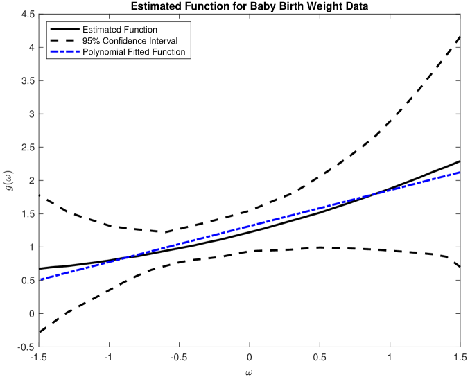
Figure 1: Estimated nonparametric link function $g(\omega)$ of the propensity score for the baby birth weight data.

We show the estimation in Figure 1 with the estimated link function in solid line and the corresponding 95% confidence interval in dashed line. We also plot the approximated second-order polynomial fitted function using the ordinary least squares estimation approach as a reference. Our results show that the estimated link function $\hat{g}$ does not seem to be an identity function. Such potential misspecification of propensity score may explain the differences for the treatment effect estimation between our estimator and the doubly robust estimator using the propensity score estimated by logistic regression. Both the estimated link function and the approximated second-order polynomial fitted function are close to each other, showing the estimation method work well in this empirical application.

7 Conclusion

To address the issue of possible misspecifications, we propose a semiparametric estimation method for the average treatment effect. Our approach assumes the propensity score function with a single-index structure, and a flexible link function is allowed. We estimate the index parameter and link function simultaneously in the infinitely dimensional function space and estimate the propensity score by implementing an optimization with the constraints of identification conditions and establish the large sample properties of our estimator. Our method is empirically applicable and can be used for models with a wide range of error distributions. Our approach also provides computational flexibility for moderately large dimension problems.

We conduct an extensive simulation study to evaluate the finite sample performance of our proposed estimator in finite samples. We provide the empirical results on the effect of maternal smoking on babies’ birth weight and the effect of the job training program on future earnings. We find that, compared to the widely used average treatment effect estimators, our approach is less prone to misspecification of the propensity score function and is valid when the propensity score approaches zero or one.

Appendix

Appendix A provides proof for Theorem 1. Appendix B gives some preliminary results about Hilbert space, Appendix C gives the proofs of the main results, Appendix D provides some additional numerical results, and Appendix E presents additional empirical application results.

Appendix A: Proof for Theorem 1

Proof of Theorem 1.

We prove the asymptotic normality of $\widehat{\Delta}_{\omega}^{ATE}$ and $\widehat{\Delta}^{ATE}$ in two steps. In the first step, we take the first-stage errors into account when estimating the propensity score function $\pi(X)$. In the second step, we prove the asymptotic properties of sample analog of treatment effects estimators.

(a) We write

$$\sqrt{N}(\widehat{\Delta}_{\omega}^{ATE}-\Delta_{\omega}^{ATE})=\Big{\{}\frac{1}{N}\sum_{i=1}^{N}\big{(}D_{i}-\hat{\pi}(X_{i})\big{)}^{2}\Big{\}}^{-1}$$

$$\times\frac{1}{\sqrt{N}}\sum_{i=1}^{N}\Big{(}Y_{i}-\Delta_{\omega}^{ATE}\big{(}D_{i}-\hat{\pi}(X_{i})\big{)}\Big{)}\big{(}D_{i}-\hat{\pi}(X_{i})\big{)}$$

$$=\Big{\{}\frac{1}{N}\sum_{i=1}^{N}\big{(}D_{i}-\hat{\pi}(X_{i})\big{)}^{2}\Big{\}}^{-1}\frac{1}{\sqrt{N}}\sum_{i=1}^{N}\Big{(}Y_{i}-\Delta_{\omega}^{ATE}\big{(}D_{i}-\pi(X_{i})\big{)}\Big{)}\big{(}D_{i}-\pi(X_{i})\big{)}$$

$$-\Big{\{}\frac{1}{N}\sum_{i=1}^{N}\big{(}D_{i}-\hat{\pi}(X_{i})\big{)}^{2}\Big{\}}^{-1}\frac{1}{\sqrt{N}}\sum_{i=1}^{N}\Delta_{\omega}^{ATE}\big{(}\pi(X_{i})-\hat{\pi}(X_{i})\big{)}\big{(}D_{i}-\pi(X_{i})\big{)}$$

$$+\Big{\{}\frac{1}{N}\sum_{i=1}^{N}\big{(}D_{i}-\hat{\pi}(X_{i})\big{)}^{2}\Big{\}}^{-1}\frac{1}{\sqrt{N}}\sum_{i=1}^{N}U_{i}\big{(}\pi(X_{i})-\hat{\pi}(X_{i})\big{)}$$

$$-\Big{\{}\frac{1}{N}\sum_{i=1}^{N}\big{(}D_{i}-\hat{\pi}(X_{i})\big{)}^{2}\Big{\}}^{-1}\frac{1}{\sqrt{N}}\sum_{i=1}^{N}\Delta_{\omega}^{ATE}\big{(}\pi(X_{i})-\hat{\pi}(X_{i})\big{)}^{2}$$

$$=A_{1N}+A_{2N}+A_{3N}+A_{4N}.$$

We first consider the asymptotic properties of $\hat{\pi}(X_{i})-\pi(X_{i})$, by the orthogonality, we write

$$\big{\|}\hat{\pi}(X_{i})-\pi(X_{i})\big{\|}_{\mathcal{L}^{2}}^{2}=\int_{\mathbb{R}}\Big{\{}\Lambda\big{(}\hat{g}_{k}(w)\big{)}-\Lambda\big{(}g_{0}(w)\big{)}\Big{\}}^{2}\pi(w)dw$$

$$\leq O(1)\int_{\mathbb{R}}\Big{\{}\big{(}\hat{g}_{k}(w)\big{)}-\big{(}g_{0}(w)\big{)}\Big{\}}^{2}\pi(w)dw=O(1)\int_{\mathbb{R}}\big{\{}H(w)(\widehat{C}_{k}-C_{0,k})+\epsilon_{0,k}\big{\}}^{2}\pi(w)dw$$

$$=O\big{(}\|\widehat{C}_{k}-C_{0,k}\|^{2}\big{)}+O\big{(}\|\epsilon_{0,k}\|^{2}_{\mathcal{L}^{2}}\big{)},$$

where the first inequality follows from the Lipschitz continuity of $\Lambda\big{(}g(w)\big{)}$, the third equality follows from the orthogonality of Hermite polynomials.

By Lemma A1 in Dong et al. (2019), we have $\|\epsilon_{0,k}\|^{2}_{\mathcal{L}^{2}}=O(k^{-r})$.

By Theorem 2.5 in Dong et al. (2019), we have $\|\widehat{C}_{k}-C_{0,k}\|^{2}=O_{P}\big{(}\frac{k}{N}\big{)}$.

Therefore, we have $\big{\|}\hat{\pi}(X_{i})-\pi(X_{i})\big{\|}_{\mathcal{L}^{2}}^{2}=O_{P}(\frac{k}{N})+O_{P}(k^{-r})$.

We next consider the asymptotic property of $\frac{1}{N}\sum_{i=1}^{N}\big{(}D_{i}-\hat{\pi}(X_{i})\big{)}^{2}$:

$$\frac{1}{N}\sum_{i=1}^{N}\big{(}D_{i}-\hat{\pi}(X_{i})\big{)}^{2}=\frac{1}{N}\sum_{i=1}^{N}\big{(}D_{i}-\pi(X_{i})\big{)}^{2}+\frac{1}{N}\sum_{i=1}^{N}\big{(}\hat{\pi}(X_{i})-\pi(X_{i})\big{)}^{2}$$

$$+\frac{2}{N}\sum_{i=1}^{N}\big{(}D_{i}-\pi(X_{i})\big{)}\big{(}\hat{\pi}(X_{i})-\pi(X_{i})\big{)}=H_{1N}+H_{2N}+H_{3N}.$$

By 2(a), we have for $H_{1N}=\frac{1}{N}\sum_{i=1}^{N}\big{(}D_{i}-\pi(X_{i})\big{)}^{2}=\mathbb{E}\big{(}D_{i}-\pi(X_{i})\big{)}^{2}+o_{P}(1)$.

Following the proofs as in $K_{11N}$ and $K_{12N}$, we have $\|H_{2N}\|=o_{P}(1)$ and $\|H_{3N}\|=o_{P}(1)$.

Therefore, we have $\frac{1}{N}\sum_{i=1}^{N}\big{(}D_{i}-\hat{\pi}(X_{i})\big{)}^{2}=\mathbb{E}\big{(}D_{i}-\pi(X_{i})\big{)}^{2}+o_{P}(1)$.

For $A_{1N}$, denote the term $\Big{(}Y_{i}-\Delta_{\omega}^{ATE}\big{(}D_{i}-\pi(X_{i})\big{)}\Big{)}\big{(}D_{i}-\pi(X_{i})\big{)}$ as $P_{i}$. By 2(a), we have $\mathbb{E}[P_{i}]=0$ and $\operatorname{Var}[P_{i}]<\infty$. Applying the Lindeberg–Levy CLT, we have:

$$A_{1N}\rightarrow_{P}N(0,\sigma_{\omega}^{2}).$$

For $A_{2N}$, we write:

$$\|A_{2N}\|=\Big{\{}\mathbb{E}\big{(}D_{i}-\pi(X_{i})\big{)}^{2}\Big{\}}^{-2}\mathbb{E}\Big{\|}\frac{1}{\sqrt{N}}\sum_{i=1}^{N}[D_{i}-\pi(X_{i})]\big{\{}\pi(X_{i})-\hat{\pi}(X_{i})\big{\}}\Big{\|}$$

$$=O(1)\frac{1}{N}\sum_{i=1}^{N}\mathbb{E}\Big{\|}\Lambda\big{(}g_{0}(X_{i}^{\prime}\theta_{0})\big{)}-\Lambda\big{(}\hat{g}_{k}(X_{i}^{\prime}\hat{\theta})\big{)}\Big{\|}$$

$$=O(1)\frac{1}{N}\sum_{i=1}^{N}\mathbb{E}\Big{\|}\Lambda\big{(}g_{0}(X_{i}^{\prime}\theta_{0})\big{)}-\Lambda\big{(}g_{0}(X_{i}^{\prime}\hat{\theta})\big{)}+\Lambda\big{(}g_{0}(X_{i}^{\prime}\hat{\theta})\big{)}-\Lambda\big{(}g_{0,k}(X_{i}^{\prime}\hat{\theta})\big{)}$$

$$+\Lambda\big{(}g_{0,k}(X_{i}^{\prime}\hat{\theta})\big{)}-\Lambda\big{(}\hat{g}_{k}(X_{i}^{\prime}\hat{\theta})\big{)}\Big{\|}\leq O(1)\frac{1}{N}\sum_{i=1}^{N}\mathbb{E}\Big{\|}\Lambda\big{(}g_{0}(X_{i}^{\prime}\theta_{0})\big{)}-\Lambda\big{(}g_{0}(X_{i}^{\prime}\hat{\theta})\big{)}\Big{\|}$$

$$+O(1)\frac{1}{N}\sum_{i=1}^{N}\mathbb{E}\Big{\|}\Lambda\big{(}g_{0}(X_{i}^{\prime}\hat{\theta})\big{)}-\Lambda\big{(}g_{0,k}(X_{i}^{\prime}\hat{\theta})\big{)}\Big{\|}+O(1)\frac{1}{N}\sum_{i=1}^{N}\mathbb{E}\Big{\|}\Lambda\big{(}g_{0,k}(X_{i}^{\prime}\hat{\theta})\big{)}-\Lambda\big{(}\hat{g}_{k}(X_{i}^{\prime}\hat{\theta})\big{)}\Big{\|}$$

$$=O(1)A_{21N}+O(1)A_{22N}+O(1)A_{23N},$$

where the second equality follows from 2(a), the fourth inequality follows from the triangular inequality.

For $A_{21N}$, we write:

$$A_{21N} =\frac{1}{N}\sum_{i=1}^{N}\mathbb{E}\Big{\|}\Lambda\big{(}g_{0}(X_{i}^{\prime}\theta_{0})\big{)}-\Lambda\big{(}g_{0}(X_{i}^{\prime}\hat{\theta})\big{)}\Big{\|}$$

$$\leq\Big{\|}\mathbb{E}\big{[}\Lambda\big{(}g_{0}(X_{i}^{\prime}\theta_{0})\big{)}-\Lambda\big{(}g_{0}(X_{i}^{\prime}\hat{\theta})\big{)}\big{]}\Big{\|}+o_{P}(1)$$

$$=\Big{\|}\mathbb{E}\big{[}\Lambda\big{(}g_{0}(X_{i}^{\prime}\theta^{*})\big{)}g_{0}^{(1)}(X_{i}^{\prime}\theta^{*})(X_{i}^{\prime}\theta_{0}-X_{i}^{\prime}\hat{\theta})\big{]}\Big{\|}+o_{P}(1)$$

$$\leq\|\hat{\theta}-\theta_{0}\|\Big{\{}\mathbb{E}\big{\|}\Lambda\big{(}g_{0}(X_{i}^{\prime}\theta^{*})\big{)}g_{0}^{(1)}(X_{i}^{\prime}\theta^{*})X_{i}X_{i}^{\prime}\big{\|}^{2}\Big{\}}^{1/2}+o_{P}(1)=o_{P}(1),$$

where the first inequality follows from 3(a), the second equality follows from mean value theorem, the third inequality follows from Cauchy-Schwarz inequality, and the last equality follows from 2(b) and the fact that $\|\hat{\theta}-\theta_{0}\|\rightarrow_{P}0$ and $\Lambda\big{(}g(X_{i}^{\prime}\theta)\big{)}$ is bounded by 1.

For $A_{22N}$, we write:

$$A_{22N}=\frac{1}{N}\sum_{i=1}^{N}\mathbb{E}\Big{\|}\Lambda\big{(}g_{0}(X_{i}^{\prime}\hat{\theta})\big{)}-\Lambda\big{(}g_{0,k}(X_{i}^{\prime}\hat{\theta})\big{)}\Big{\|}\leq O(1)\Big{\|}\mathbb{E}\big{[}\Lambda\big{(}g_{0}(X_{i}^{\prime}\hat{\theta})\big{)}-\Lambda\big{(}g_{0,k}(X_{i}^{\prime}\hat{\theta})\big{)}\big{]}\Big{\|}+o_{P}(1)$$

$$\leq O(1)\Big{\|}\mathbb{E}\big{[}\epsilon_{0,k}(X_{i}^{\prime}\hat{\theta})\big{]}\Big{\|}+o_{P}(1)\leq O(1)\Big{\{}\mathbb{E}\big{\|}\epsilon_{0,k}(X_{i}^{\prime}\hat{\theta})\big{\|}^{2}\Big{\}}^{1/2}+o_{P}(1)=o_{P}(1),$$

where the first inequality follows from 3(a), the second inequality follows from Lipschitz continuity of $\Lambda(g(X_{i}^{\prime}\theta))$, the third inequality follows from Cauchy-Schwarz inequality, and the last equality follows from 3(c) and Lemma A1 from Dong et al. (2019).

For $A_{23N}$, we write

$$A_{23N}=\frac{1}{N}\sum_{i=1}^{N}\mathbb{E}\Big{\|}\Lambda\big{(}g_{0,k}(X_{i}^{\prime}\hat{\theta})\big{)}-\Lambda\big{(}\hat{g}_{k}(X_{i}^{\prime}\hat{\theta})\big{)}\Big{\|}$$

$$\leq\Big{\|}\mathbb{E}\big{\{}\Lambda\big{(}H(X_{i}^{\prime}\hat{\theta})^{\prime}C_{0,k}\big{)}-\Lambda\big{(}H(X_{i}^{\prime}\hat{\theta})^{\prime}\widehat{C}_{k}\big{)}\big{\}}\Big{\|}+o_{P}(1)\leq O(1)\Big{\|}\mathbb{E}\big{[}H(X_{i}^{\prime}\hat{\theta})^{\prime}(\widehat{C}_{k}-C_{0,k})\big{]}\Big{\|}+o_{P}(1)$$

$$\leq O(1)\Big{\{}(\widehat{C}_{k}-C_{0,k})^{\prime}\mathbb{E}\big{[}H(X_{i}^{\prime}\hat{\theta})H(X_{i}^{\prime}\hat{\theta})^{\prime}\big{]}(\widehat{C}_{k}-C_{0,k})\Big{\}}^{1/2}$$

$$\leq O(1)\|\widehat{C}_{k}-C_{0,k}\|+o_{P}(1)\leq O(1)\|\hat{g}_{k}-g_{0}\|_{\mathcal{L}^{2}}+o_{P}(1)=o_{P}(1),$$

where the first inequality follows from 3(a), the second inequality follows from Lipschitz continuity of $\Lambda\big{(}g(X_{i}^{\prime}\theta)\big{)}$, the third inequality follows from Cauchy-Schwarz inequality, the fourth inequality follows from Lemma A4 in Dong et al. (2019), and the last inequality follows from the definition of $\|\cdot\|_{\mathcal{L}^{2}}$.

For $A_{3N}$, we write:

$$\|A_{3N}\|= \Big{\{}\mathbb{E}\big{(}D_{i}-\pi(X_{i})\big{)}^{2}\Big{\}}^{-2}\mathbb{E}\Big{\|}\frac{1}{\sqrt{N}}\sum_{i=1}^{N}U_{i}\big{\{}\pi(X_{i})-\hat{\pi}(X_{i})\big{\}}\Big{\|}$$

$$= O(1)\frac{1}{N}\sum_{i=1}^{N}\mathbb{E}\Big{\|}U_{i}\Big{\{}\Lambda\big{(}g_{0}(X_{i}^{\prime}\theta_{0})\big{)}-\Lambda\big{(}\hat{g}_{k}(X_{i}^{\prime}\hat{\theta})\big{)}\Big{\}}\Big{\|}$$

$$= O(1)\frac{1}{N}\sum_{i=1}^{N}\mathbb{E}\Big{\|}U_{i}\Big{\{}\Lambda\big{(}g_{0}(X_{i}^{\prime}\theta_{0})\big{)}-\Lambda\big{(}g_{0}(X_{i}^{\prime}\hat{\theta})\big{)}\Big{\}}+U_{i}\Big{\{}\Lambda\big{(}g_{0}(X_{i}^{\prime}\hat{\theta})\big{)}-\Lambda\big{(}g_{0,k}(X_{i}^{\prime}\hat{\theta})\big{)}\Big{\}}$$

$$+ U_{i}\Big{\{}\Lambda\big{(}g_{0,k}(X_{i}^{\prime}\hat{\theta})\big{)}-\Lambda\big{(}\hat{g}_{k}(X_{i}^{\prime}\hat{\theta})\big{)}\Big{\}}\Big{\|}=o_{P}(1),$$

where the second equality follows from 2(a), the fourth inequality follows from the triangular inequality and similar proofs as $A_{2N}$.

For $A_{4N}$, we write:

$$\|A_{4N}\|= \Big{\{}\mathbb{E}\big{(}D_{i}-\pi(X_{i})\big{)}^{2}\Big{\}}^{-2}\mathbb{E}\Big{\|}\frac{1}{\sqrt{N}}\sum_{i=1}^{N}\Delta_{\omega}^{ATE}\big{(}\pi(X_{i})-\hat{\pi}(X_{i})\big{)}^{2}\Big{\|}$$

$$= O(1)\frac{1}{N}\sum_{i=1}^{N}\mathbb{E}\Big{\|}\big{\{}\Lambda\big{(}g_{0}(X_{i}^{\prime}\theta_{0})\big{)}-\Lambda\big{(}\hat{g}_{k}(X_{i}^{\prime}\theta_{0})\big{)}\big{\}}^{2}\Big{\|}$$

$$\leq O(1)\frac{1}{N}\sum_{i=1}^{N}\mathbb{E}\Big{\|}\big{\{}\Lambda\big{(}g_{0}(X_{i}^{\prime}\theta_{0})\big{)}-\Lambda\big{(}g_{0}(X_{i}^{\prime}\hat{\theta})\big{)}\big{\}}^{2}\Big{\|}$$

$$+O(1)\frac{1}{N}\sum_{i=1}^{N}\mathbb{E}\Big{\|}\big{\{}\Lambda\big{(}g_{0}(X_{i}^{\prime}\hat{\theta})\big{)}-\Lambda\big{(}g_{0,k}(X_{i}^{\prime}\hat{\theta})\big{)}\big{\}}^{2}\Big{\|}$$

$$+ O(1)\frac{1}{N}\sum_{i=1}^{N}\mathbb{E}\Big{\|}\big{\{}\Lambda\big{(}g_{0,k}(X_{i}^{\prime}\hat{\theta})\big{)}-\Lambda\big{(}\hat{g}_{k}(X_{i}^{\prime}\hat{\theta})\big{)}\big{\}}^{2}\Big{\|}=o_{P}(1),$$

where the second equality comes from the boundness of $\Delta_{\omega}^{ATE}$, the third inequality comes from triangular inequality, and the fourth equality comes from the similar proofs as $A_{2N}$.

In sum, we have shown the following asymptotic normality:

$$\sqrt{N}(\widehat{\Delta}_{\omega}^{ATE}-\Delta_{\omega}^{ATE})\rightarrow_{D}N(0,\sigma_{\omega}^{2}).$$

(b) We write:

$$\sqrt{N}(\widehat{\Delta}^{ATE}-\Delta^{ATE})=\Big{\{}\frac{1}{N}\sum_{i=1}^{N}\hat{\upsilon}(X_{i})^{-1}\big{(}D_{i}-\hat{\pi}(X_{i})\big{)}^{2}\Big{\}}^{-1}$$

$$\times\frac{1}{\sqrt{N}}\sum_{i=1}^{N}\hat{\upsilon}(X_{i})^{-1}\big{(}Y_{i}-\Delta^{ATE}(D_{i}-\hat{\pi}(X_{i})\big{)}\big{(}D_{i}-\hat{\pi}(X_{i})\big{)}$$

$$=\Big{\{}\frac{1}{N}\sum_{i=1}^{N}\hat{\upsilon}(X_{i})^{-1}\big{(}D_{i}-\hat{\pi}(X_{i})\big{)}^{2}\Big{\}}^{-1}\frac{1}{\sqrt{N}}\sum_{i=1}^{N}\hat{\upsilon}(X_{i})^{-1}\big{(}Y_{i}-\Delta^{ATE}(D_{i}-\pi(X_{i})\big{)}\big{(}D_{i}-\pi(X_{i})\big{)}$$

$$-\Big{\{}\frac{1}{N}\sum_{i=1}^{N}\hat{\upsilon}(X_{i})^{-1}\big{(}D_{i}-\hat{\pi}(X_{i})\big{)}^{2}\Big{\}}^{-1}\frac{1}{\sqrt{N}}\sum_{i=1}^{N}\hat{\upsilon}(X_{i})^{-1}\Delta^{ATE}\big{(}\pi(X_{i})-\hat{\pi}(X_{i})\big{)}\big{(}D_{i}-\pi(X_{i})\big{)}$$

$$+\Big{\{}\frac{1}{N}\sum_{i=1}^{N}\hat{\upsilon}(X_{i})^{-1}\big{(}D_{i}-\hat{\pi}(X_{i})\big{)}^{2}\Big{\}}^{-1}\frac{1}{\sqrt{N}}\sum_{i=1}^{N}\hat{\upsilon}(X_{i})^{-1}U_{i}\big{(}\pi(X_{i})-\hat{\pi}(X_{i})\big{)}$$

$$-\Big{\{}\frac{1}{N}\sum_{i=1}^{N}\hat{\upsilon}(X_{i})^{-1}\big{(}D_{i}-\hat{\pi}(X_{i})\big{)}^{2}\Big{\}}^{-1}\frac{1}{\sqrt{N}}\sum_{i=1}^{N}\hat{\upsilon}(X_{i})^{-1}\Delta^{ATE}\big{(}\pi(X_{i})-\hat{\pi}(X_{i})\big{)}^{2}$$

$$=B_{1N}+B_{2N}+B_{3N}+B_{4N}.$$

Following similar derivations to those used for $\frac{1}{N}\sum_{i=1}^{N}\big{(}D_{i}-\hat{\pi}(X_{i})\big{)}^{2}$, we have

$$\frac{1}{N}\sum_{i=1}^{N}\hat{\upsilon}(X_{i})^{-1}\big{(}D_{i}-\hat{\pi}(X_{i})\big{)}^{2}\rightarrow_{P}\mathbb{E}\Big{[}\upsilon(X_{i})^{-1}\big{(}D_{i}-\pi(X_{i})\big{)}^{2}\Big{]}.$$

For $B_{1N}$, denote the term $\Big{(}Y_{i}-\Delta^{ATE}\big{(}D_{i}-\pi(X_{i})\big{)}\Big{)}\big{(}D_{i}-\pi(X_{i})\big{)}$ as $P_{i}$. By 2(a), we have $\mathbb{E}[P_{i}]=0$ and $\operatorname{Var}[P_{i}]<\infty$. Applying the Lindeberg–Levy CLT, we have:

$$B_{1N}\rightarrow_{P}N(0,\sigma^{2}).$$

For $B_{2N}$, we write

$$\|B_{2N}\|=\Big{\{}\mathbb{E}\big{[}\upsilon(X_{i})^{-1}\big{(}D_{i}-\pi(X_{i})\big{)}^{2}\big{]}\Big{\}}^{-2}$$

$$\mathbb{E}\Big{\|}\frac{1}{\sqrt{N}}\sum_{i=1}^{N}\hat{\upsilon}(X_{i})^{-1}\Delta^{ATE}\big{(}\pi(X_{i})-\hat{\pi}(X_{i})\big{)}\big{(}D_{i}-\pi(X_{i})\big{)}\Big{\|}$$

$$\leq O(1)\frac{1}{N}\sum_{i=1}^{N}\mathbb{E}\Big{\|}\Lambda\big{(}g_{0}(X_{i}^{\prime}\theta_{0})\big{)}-\Lambda\big{(}\hat{g}_{k}(X_{i}^{\prime}\hat{\theta})\big{)}\Big{\|}=o_{P}(1),$$

where the second inequality follows from 2(a) and boundness of $\upsilon(\cdot)$, and the third equality follows from the similar proofs as $A_{2N}$.

For $B_{3N}$, we write:

$$\|B_{3N}\|= \Big{\{}\mathbb{E}\big{[}\upsilon(X_{i})^{-1}\big{(}D_{i}-\pi(X_{i})\big{)}^{2}\big{]}\Big{\}}^{-2}\mathbb{E}\Big{\|}\frac{1}{\sqrt{N}}\sum_{i=1}^{N}\hat{\upsilon}(X_{i})^{-1}U_{i}\big{\{}\pi(X_{i})-\hat{\pi}(X_{i})\big{\}}\Big{\|}$$

$$\leq O(1)\frac{1}{N}\sum_{i=1}^{N}\mathbb{E}\Big{\|}U_{i}\big{\{}\Lambda\big{(}g_{0}(X_{i}^{\prime}\theta_{0})\big{)}-\Lambda\big{(}\hat{g}_{k}(X_{i}^{\prime}\hat{\theta})\big{)}\big{\}}\Big{\|}=o_{P}(1),$$

where the second inequality follows from 2(a) and boundness of $\upsilon(\cdot)$, and the third equality follows from the similar proofs as $A_{3N}$.

For $B_{4N}$, we write:

$$\|B_{4N}\|= \Big{\{}\mathbb{E}\big{[}\upsilon(X_{i})^{-1}\big{(}D_{i}-\pi(X_{i})\big{)}^{2}\big{]}\Big{\}}^{-2}\mathbb{E}\Big{\|}\frac{1}{\sqrt{N}}\sum_{i=1}^{N}\hat{\upsilon}(X_{i})^{-1}\Delta_{\omega}^{ATE}\big{(}\pi(X_{i})-\hat{\pi}(X_{i})\big{)}^{2}\Big{\|}$$

$$\leq O(1)\frac{1}{N}\sum_{i=1}^{N}\mathbb{E}\Big{\|}\Lambda\big{(}g_{0}(X_{i}^{\prime}\theta_{0})\big{)}-\Lambda\big{(}\hat{g}_{k}(X_{i}^{\prime}\hat{\theta})\big{)}\Big{\|}=o_{P}(1),$$

where the second inequality follows from 2(a) and boundedness of $\upsilon(\cdot)$, and the third equality follows from the similar proofs as $A_{4N}$.

In sum, we have:

$$\sqrt{N}(\widehat{\Delta}^{ATE}-\Delta^{ATE})\rightarrow_{D}N(0,\sigma^{2}),$$

which completes the proof of Theorem 1.

∎

Appendix B: Preliminary properties for Hilbert Space

In this section, we present the properties of the Hilbert Space $\mathcal{L}^{2}$ that includes all polynomials, all power functions, all bounded functions, and even some exponential functions. More importantly, all functions in the space are defined on the entire real line.

An inner product for $g_{1}(w),g_{2}(w)\in\mathcal{L}^{2}$ is given by:

$$\langle g_{1}(w),g_{2}(w)\rangle=\int g_{1}(w)g_{2}(w)\exp(-w^{2}/2)dw.$$

Hermite polynomials form a complete orthogonal sequence in $\mathcal{L}^{2}$ with each elements defined by:

$$h_{m}(w):=\frac{1}{\sqrt{m!}}\cdot(-1)^{m}\cdot\exp(w^{2}/2)\cdot\frac{d^{m}}{dw^{m}}\exp(-w^{2}/2),$$

for $m=0,1,2,\dots$.

The orthogonality of this basis system satisfies $\int h_{m}(w)h_{n}(w)\exp(-w^{2}/2)dw=\sqrt{2\pi}\delta_{mn}$, where $\delta_{mn}$ is the Kronecker delta. For $\forall g(w)\in\mathcal{L}^{2}$, we have orthogonal series expansion:

$$g(w)=\sum_{j=1}^{\infty}c_{j}h_{j}(w),\quad c_{j}=\langle g(w),h_{j}(w)\rangle.$$

For any truncation parameter $k\geq 1$, we split the orthogonal series expansion into two parts as following:

$$g(w)=g_{k}(w)+\epsilon_{k}(w),$$ (B.1)

where $g_{k}(w):=H(w)^{\prime}C_{k}$, $H(w)=\big{(}h_{1}(w),\ldots,h_{k}(w)\big{)}^{\prime}$, $C_{k}=(c_{1},\ldots,c_{k})^{\prime}$, and the approximation residual is given by $\epsilon_{k}(w)=\sum_{j=k+1}^{\infty}c_{j}h_{j}(w)$.

The quantity of $\|H(w)\|$ is crucial for the asymptotic properties of our estimators, using the results in the Theorem 1.1 of Levin and Lubinsky (1992) and Dong et al. (2021), we have:

$$\frac{1}{\sqrt{k}}\sum_{j=1}^{k}h_{j}^{2}(w)\asymp\exp(w^{2})\left(\max\left\{k^{-2/3},1-\frac{|w|}{2\sqrt{k}}\right\}\right)^{1/2},$$

uniformly for $k\geq 1$ and $w\in\{u:|u|\leq\sqrt{2k}(1+Lk^{-2/3})\},$ where $L>0$ is given. In addition, we can show that the order of $\|H(w)\|$ is $O(\sqrt{k})$ when the condition for $1-|x|/\sqrt{2k}>k^{-2/3}$ satisfies as long as the truncation parameter $k$ diverge.

Appendix C: Proofs for the main results and other results

Proof of Lemma 2.1.

(a) We have $\mathbb{E}[\operatorname{var}(D|X)]>0$ under 1(b), and thus the regression parameter $\beta$ can be written as:

$$\beta=\frac{\mathbb{E}\big{[}\big{(}D-\pi(X)\big{)}Y\big{]}}{\mathbb{E}[\operatorname{var}(D|X)]}.$$

Given 1(a) and that $Y=DY(1)+(1-D)Y(0)$, we have:

$$\mathbb{E}[DY|X]=\pi(X)\mathbb{E}[Y(1)|X]\ \ \ \mathrm{and}\ \ \ \mathbb{E}[Y|X]=\pi(X)\mathbb{E}[Y(1)|X]+\big{(}1-\pi(X)\big{)}\mathbb{E}[Y(0)|X].$$

It follows from the law of iterated expectation that:

$$\beta=\frac{\mathbb{E}[\pi(X)\{1-\pi(X)\}\mathbb{E}(Y(1)-Y(0)|X)]}{\mathbb{E}[\operatorname{var}(D|X)]}.$$

This leads to the desired result.

(b) Under 1(b) and the law of iterated expectation, $\mathbb{E}[\upsilon(X)\operatorname{var}(D|X)]=1$ and thus the regression parameter $\gamma$ can be written as:

$$\gamma=\frac{\mathbb{E}[\upsilon(X)\big{(}D-\pi(X)\big{)}Y]}{\mathbb{E}[\upsilon(X)\operatorname{var}(D|X)]}.$$

Given the unconfoundedness under 1(a) and that $Y=DY(1)+(1-D)Y(0)$, we have:

$$\mathbb{E}[\upsilon(X)DY|X]=\frac{\mathbb{E}[Y(1)|X]}{1-\pi(X)}\ \ \ \mathrm{and}\ \ \ \mathbb{E}[\upsilon(X)\pi(X)Y|X]=\frac{\pi(X)\mathbb{E}[Y(1)|X]}{1-\pi(X)}+\mathbb{E}[Y(0)|X].$$

Thus, the desired result follows. ∎

In addition to the main results established in Section 4 of the submission, we have the following important results. The following lemma establishes the consistency of the estimators $(\hat{\theta},\widehat{g}_{k})$.

Lemma C.1: Define the norm $\big{\|}(\theta,g)\big{\|}_{2}:=\big{(}\|\theta\|^{2}+\|g\|^{2}\big{)}^{1/2}$ over the space $\Theta\times\mathcal{L}^{2}$. Suppose that 2 holds. Then, we have, as $N\rightarrow\infty$,

$$\big{\|}(\hat{\theta},\widehat{g}_{k})-(\theta_{0},g_{0})\big{\|}_{2}\rightarrow_{p}0.$$

In Lemma C.2 below, we establish the convergence rate and the limit distribution of the estimator $\hat{\theta}$. To present the result, let $P_{\theta_{0}}:=I_{d}-\theta_{0}\theta_{0}^{\prime}$ be a $d\times d$ matrix. Under the constraint of $\|\theta_{0}\|=1$, $P_{\theta_{0}}$ can be considered as the projection matrix that maps any $d\times 1$ vector into the orthogonal complement space of true parameter $\theta_{0}$. Let $V:=[v_{1},\dots,v_{d-1}]$ be a $d\times(d-1)$ matrix consisting of eigenvectors $v_{j}$ associated with eigenvalue of 1.

Lemma C.2: Let Assumptions 2 and 3 hold. Then, as $N\rightarrow\infty$,

1. $\sqrt{N}V^{\prime}(\hat{\theta}-\theta_{0})\rightarrow_{D}N\big{(}0,(V^{\prime}QV)^{-1}V^{\prime}WV(V^{\prime}QV)^{-1}\big{)},$

2. $\theta_{0}^{\prime}(\hat{\theta}-\theta_{0})=O_{p}(1/N)$,

where $Q:=\mathbb{E}\big{[}\big{\{}g_{0}^{(1)}(X^{\prime}\theta_{0})\big{\}}^{2}XX^{\prime}\big{]}$ and $W:=\mathbb{E}\big{[}\big{(}D-\pi(X)\big{)}^{2}\big{\{}g_{0}^{(1)}(X^{\prime}\theta_{0})\big{\}}^{2}XX^{\prime}\big{]}$.

Lemma C.2(a) establishes the asymptotic normality of $V^{\prime}(\hat{\theta}-\theta_{0})$ that utilizes the transformation of $\hat{\theta}-\theta_{0}$ into $\mathbb{R}^{d-1}$ as both $\hat{\theta}$ and $\theta_{0}$ belongs to the unit ball of $\mathbb{R}^{d-1}$. Lemma C.2(b) is due to the constraint of $\|\theta_{0}\|=1$. It measures the distance of $\hat{\theta}$ to the surface of unit ball and indicates that along the direction of true value $\theta_{0}$, the estimated value $\hat{\theta}$ converges with a faster rate than in all other directions that are orthogonal to true value $\theta_{0}$.

Proof of Lemma C.1.

Note that the objective function $\ell_{N}\big{(}\check{\theta},\{c_{j}\}_{j=1}^{k}\big{)}$ in Equation (5) is interchangeable with the sample version of population objective function $\ell_{N}(\theta,g)$.

Our proof is composited of two parts. In the first part, we prove the convergence of sample objective function $\ell_{N}(\theta,g)$ to the population objective $\ell(\theta,g)$ using Lemma A2 in Newey and Powell (2003). In the second part, we prove the consistency of $(\hat{\theta},\widehat{g}_{k})$ by contradiction.

(a) We begin to prove the convergence of sample objective function $\ell_{N}(\theta,g)$ to the population objective $\ell(\theta,g)$:

$$\max_{\Theta\times G}|\ell_{N}(\theta,g)-\ell(\theta,g)|\rightarrow_{P}0.$$

We proceed by checking whether Conditions (i) to (iii) in Lemma A2 of Newey and Powell (2003) hold.

For Condition (i), as we assume that $\Theta$ is a compact subset of the parameter space $\mathbb{R}^{d}$ and $\Theta$ is defined with norm. Therefore, Condition (i) holds.

For Condition (ii), as we assume that the data generating process is independent and identically distributed in 2(a), therefore, we apply the Law of Large Numbers (LLN) and show that:

$$\ell_{N}(\theta,g)=\ell(\theta,g)\big{(}1+o_{P}(1)\big{)}.$$

Therefore, Condition (ii) holds.

For Condition (iii), we prove by showing the continuity of $\ell(\theta,g)$ holds, which indicates that the continuity of $\ell_{N}(\theta,g)$ holds with probability approaching 1.

For any given $(\theta_{1},g_{1})$ and $(\theta_{2},g_{2})$ belonging to $\Theta\times G$, we have:

$$\big{|}\ell(\theta_{1},g_{1})-\ell(\theta_{2},g_{2})\big{|}\leq\big{|}\ell(\theta_{1},g_{1})-\ell(\theta_{1},g_{2})\big{|}+\big{|}\ell(\theta_{1},g_{2})-\ell(\theta_{2},g_{2})\big{|}=A_{1}+A_{2}.$$

For $A_{1}$, we have:

$$\big{|}\ell(\theta_{1},g_{1})-\ell(\theta_{1},g_{2})\big{|}=\Big{|}\mathbb{E}\big{[}D_{i}g_{1}(X_{i}^{\prime}\theta_{1})-D_{i}g_{2}(X_{i}^{\prime}\theta_{1})+\ln\big(1+e^{g_{2}(X_{i}^{\prime}\theta_{1})}\big{missing})-\ln\big(1+e^{g_{1}(X_{i}^{\prime}\theta_{1})}\big{missing})\big{]}\Big{|}$$

$$\leq O(1)\big{\{}\mathbb{E}\big{[}g_{1}(X_{i}^{\prime}\theta_{1})-g_{2}(X_{i}^{\prime}\theta_{1})\big{]}^{2}\big{\}}^{1/2}+\big{\{}\mathbb{E}\big{[}\ln\big(1+e^{g_{2}(X_{i}^{\prime}\theta_{1})}\big{missing})-\ln\big(1+e^{g_{1}(X_{i}^{\prime}\theta_{1})}\big{missing})\big{]}^{2}\big{\}}^{1/2}$$

$$=A_{11}+A_{12},$$

where the second inequality follows from the fact that $D_{i}$ is a binary variable and the Cauchy-Schwarz inequality.

For $A_{11}$, we have:

$$\mathbb{E}[g_{1}(X_{i}^{\prime}\theta_{1})-g_{2}(X_{i}^{\prime}\theta_{1})]^{2}=\int\big{(}g_{1}(w)-g_{2}(w)\big{)}^{2}f_{\theta_{1}}(w)dw$$

$$=\int\big{(}g_{1}(w)-g_{2}(w)\big{)}^{2}\exp(-w^{2}/2)\cdot\exp(w^{2}/2)f_{\theta_{1}}(w)dw$$

$$\leq M\int\big{(}g_{1}(w)-g_{2}(w)\big{)}^{2}\exp(-w^{2}/2)dw=M\|g_{1}-g_{2}\|_{\mathcal{L}^{2}}^{2},$$

where the inequality follows from 2(b) due to $\sup_{\{(\theta,w)\in\Theta\times\mathbb{R}\}}\exp(w^{2}/2)f_{\theta}(w)\leq M$.

For $A_{12}$, note that $\forall a,b>0$, we have:

$$\big{|}\ln(1+a)-\ln(1+b)\big{|}<\big{|}\ln(a)-\ln(b)\big{|}.$$

Therefore, we have:

$$\mathbb{E}\big{[}\ln\big(1+e^{g_{2}(X_{i}^{\prime}\theta_{1})}\big{missing})-\ln\big(1+e^{g_{1}(X_{i}^{\prime}\theta_{1})}\big{missing})\big{]}^{2} \leq\mathbb{E}\big{[}g_{2}(X_{i}^{\prime}\theta_{1})-g_{1}(X_{i}^{\prime}\theta_{1})\big{]}^{2}$$

$$\leq M\|g_{1}-g_{2}\|_{\mathcal{L}^{2}}^{2}.$$

For $A_{1}$, we have shown:

$$\big{|}\ell(\theta_{1},g_{1})-\ell(\theta_{1},g_{2})\big{|}\leq O(1)\|g_{1}-g_{2}\|_{\mathcal{L}^{2}}.$$ (C.2)

For $A_{2}$, we write:

$$\big{|}\ell(\theta_{1},g_{2})-\ell(\theta_{2},g_{2})\big{|}=\Big{|}\mathbb{E}\big{[}D_{i}g_{2}(X_{i}^{\prime}\theta_{1})-D_{i}g_{2}(X_{i}^{\prime}\theta_{2})+\ln\big(1+e^{g_{2}(X_{i}^{\prime}\theta_{2})}\big{missing})-\ln\big(1+e^{g_{2}(X_{i}^{\prime}\theta_{1})}\big{missing})\big{]}\Big{|}$$

$$\leq O(1)\big{\{}\mathbb{E}\big{[}g_{2}(X_{i}^{\prime}\theta_{1})-g_{2}(X_{i}^{\prime}\theta_{2})\big{]}^{2}\big{\}}^{1/2}+\big{\{}\mathbb{E}\big{[}\ln\big(1+e^{g_{2}(X_{i}^{\prime}\theta_{2})}\big{missing})-\ln\big(1+e^{g_{2}(X_{i}^{\prime}\theta_{1})}\big{missing})\big{]}^{2}\big{\}}^{1/2}$$

$$=A_{21}+A_{22},$$

where the inequality follows from the fact that $D_{i}$ is a binary variable and Cauchy-Schwarz inequality.

Let $\theta^{*}$ lie between $\theta_{1}$ and $\theta_{2}$, and for $A_{21}$, and write

$$\mathbb{E}\big{[}g_{2}(X_{i}^{\prime}\theta_{1})-g_{2}(X_{i}^{\prime}\theta_{2})\big{]}^{2}=\mathbb{E}\big{[}(\theta_{2}-\theta_{1})^{\prime}X_{i}X_{i}^{\prime}(\theta_{2}-\theta_{1})\{g_{2}^{(1)}(X_{i}^{\prime}\theta^{*})\}^{2}\big{]}$$

$$\leq\|\theta_{2}-\theta_{1}\|^{2}\mathbb{E}\big{\|}X_{i}X_{i}^{\prime}\{g_{2}^{(1)}(X_{i}^{\prime}\theta^{*})\}^{2}\big{\|}\leq O(1)\|\theta_{2}-\theta_{1}\|^{2},$$

where the second inequality follows from 2(b).

Note that for $A_{22}$, we write:

$$\mathbb{E}\big{[}\ln\big(1+e^{g_{2}(X_{i}^{\prime}\theta_{2})}\big{missing})-\ln\big(1+e^{g_{2}(X_{i}^{\prime}\theta_{1})}\big{missing})\big{]}^{2}$$

$$=\mathbb{E}\big{[}(\theta_{2}-\theta_{1})^{\prime}X_{i}X_{i}^{\prime}(\theta_{2}-\theta_{1})\times\big{\{}\Lambda\big{(}g_{2}(X_{i}^{\prime}\theta^{*})\big{)}g_{2}^{(1)}(X_{i}^{\prime}\theta^{*})\big{\}}^{2}\big{]}$$

$$\leq\|\theta_{2}-\theta_{1}\|^{2}\times\mathbb{E}\big{\|}X_{i}X_{i}^{\prime}\{\Lambda\big{(}g_{2}(X_{i}^{\prime}\theta^{*})\big{)}g_{2}^{(1)}(X_{i}^{\prime}\theta^{*})\}^{2}\big{\|}\leq O(1)\|\theta_{2}-\theta_{1}\|^{2},$$

where the second inequality follows from the fact that $\big{\|}\Lambda\big{(}g(X_{i}^{\prime}\theta)\big{)}\big{\|}\leq 1$ and 2(b).

For $A_{2}$, we have shown:

$$\big{|}\ell(\theta_{1},g_{2})-\ell(\theta_{2},g_{2})\big{|}\leq O(1)\|\theta_{2}-\theta_{1}\|.$$ (C.3)

Combining Equations C.2 and C.3, we obtain:

$$\big{|}\ell(\theta_{1},g_{1})-\ell(\theta_{2},g_{2})\big{|}\leq O(1)\big{\|}(\theta_{1},g_{1})-(\theta_{2},g_{2})\big{\|}_{2},$$

which indicates the continuity of $\ell(\theta,g)$. Therefore, Condition (iii) of Lemma A2 of Newey and Powell (2003) holds. We then have shown $\max_{\Theta\times G}\big{|}\ell_{N}(\theta,g)-\ell(\theta,g)\big{|}\rightarrow_{P}0$.

(b) We next show the consistency of $(\hat{\theta},\widehat{g}_{k})$ by contradiction. By definition of $(\hat{\theta},\widehat{g}_{k})$, regardless of the value of $\lambda$, we have:

$$\ell_{N}(\hat{\theta},\widehat{g}_{k})-\ell_{N}(\theta_{0},g_{0})>0.$$

By the uniform convergence and the continuity of $\ell(\theta,g)$, if $(\hat{\theta},\widehat{g}_{k})\nrightarrow_{P}(\theta_{0},g_{0})$, we have:

$$\ell_{N}(\theta_{0},g_{0})-\ell_{N}(\hat{\theta},\widehat{g}_{k})>0,$$

with probability approaching 1, which contradicts the definition of $(\hat{\theta},\widehat{g}_{k})$ as the maximizer for the sample version of objective function.

Therefore, we have $\big{\|}(\hat{\theta},\widehat{g}_{k})-(\theta_{0},g_{0})\big{\|}_{2}\rightarrow_{P}0$.

∎

Proof of Lemma C.2.

To simplify the notation, we denote the constrained maximization objective function in Equation (5) with:

$$\mathcal{W}_{N}(\theta,C_{k},\lambda):=\frac{1}{N}\ell_{N}\big{(}\theta,\left\{c_{j}\right\}_{j=1}^{k}\big{)}+\lambda\big{(}\|\theta\|^{2}-1\big{)},$$

where $\lambda$ is the Lagrange multiplier.

We prove the asymptotic normality of $\hat{\theta}$ in two parts. In the first part, we use the routine procedure in Yu and Ruppert (2002) to study the objective function $\mathcal{W}_{N}(\theta,C_{k},\lambda)$. In the second part, we analyze the asymptotic property of each function used in this procedure.

(1) In the first part, by the definition of $(\hat{\theta},\left\{\hat{c}_{j}\right\}_{j=1}^{k})$, we have:

$$\partialderivative{\mathcal{W}_{N}(\hat{\theta},\widehat{C}_{k},\hat{\lambda})}{\theta}=0,\ \ \partialderivative{\mathcal{W}_{N}(\hat{\theta},\widehat{C}_{k},\hat{\lambda})}{C_{k}}=0,\ \ \partialderivative{\mathcal{W}_{N}(\hat{\theta},\widehat{C}_{k},\hat{\lambda})}{\lambda}=0.$$

By multiplying $\hat{\theta}$ in both sides of $\partialderivative*{\mathcal{W}_{N}(\hat{\theta},\widehat{C}_{k},\hat{\lambda})}{\theta}=0$, we have:

$$\hat{\lambda}=\frac{1}{2N}\sum_{i=1}^{N}\big{[}D_{i}-\Lambda\big{(}\hat{g}_{k}(X_{i}^{\prime}\hat{\theta})\big{)}\big{]}\hat{g}_{k}^{(1)}(X_{i}^{\prime}\hat{\theta})X_{i}^{\prime}\hat{\theta}.$$

Multiplying $V^{\prime}$ to both sides of $\partialderivative*{\mathcal{W}_{N}(\hat{\theta},\widehat{C}_{k},\hat{\lambda})}{\theta}=0$, we have:

$$0=V^{\prime}\partialderivative{\mathcal{W}_{N}(\hat{\theta},\widehat{C}_{k},\hat{\lambda})}{\theta}=V^{\prime}\partialderivative{\mathcal{W}_{N}(\theta_{0},\widehat{C}_{k},\hat{\lambda})}{\theta}+V^{\prime}\partialderivative{\mathcal{W}_{N}(\bar{\theta},\widehat{C}_{k},\hat{\lambda})}{\theta}{\theta^{\prime}}(\hat{\theta}-\theta_{0})$$

$$=V^{\prime}\partialderivative{\mathcal{W}_{N}(\theta_{0},\widehat{C}_{k},\hat{\lambda})}{\theta}+V^{\prime}\partialderivative{\mathcal{W}_{N}(\bar{\theta},\widehat{C}_{k},\hat{\lambda})}{\theta}{\theta^{\prime}}(VV^{\prime}+\theta_{0}\theta_{0}^{\prime})(\hat{\theta}-\theta_{0})$$

$$=V^{\prime}\partialderivative{\mathcal{W}_{N}(\theta_{0},\widehat{C}_{k},\hat{\lambda})}{\theta}+V^{\prime}\partialderivative{\mathcal{W}_{N}(\bar{\theta},\widehat{C}_{k},\hat{\lambda})}{\theta}{\theta^{\prime}}VV^{\prime}(\hat{\theta}-\theta_{0})-\frac{1}{2}\|\hat{\theta}-\theta_{0}\|^{2}V^{\prime}\partialderivative{\mathcal{W}_{N}(\bar{\theta},\widehat{C}_{k},\hat{\lambda})}{\theta}{\theta^{\prime}}\theta_{0},$$

where the second equality follows from Taylor expansion with $\overline{\theta}$ lies between $\theta_{0}$ and $\hat{\theta}$, the third equality follows from $I_{d}=P_{\theta_{0}}+\theta_{0}\theta_{0}^{\prime}=VV^{\prime}+\theta_{0}\theta_{0}^{\prime}$, and the fourth equality follows from $\hat{\theta}^{\prime}\theta_{0}-1=-\|\hat{\theta}-\theta_{0}\|^{2}+(1-\hat{\theta}^{\prime}\theta_{0})$.

(2) In the second part, we analyze the asymptotic property of $\partialderivative*{\mathcal{W}_{N}(\theta,C_{k},\lambda)}{\theta}{\theta^{\prime}}$ and $\partialderivative*{\mathcal{W}_{N}(\theta,C_{k},\lambda)}{\theta}$ used in the above procedure. Similar to the proofs in Lemma C.1, it is easy to show $\big{\|}(\bar{\theta},\widehat{g}_{k})-(\theta_{0},g_{0})\big{\|}_{2}\rightarrow_{P}0$. We therefore focus on a sufficiently small neighborhood of $(\theta_{0},g_{0})$ in the following proof.

In the following proofs, we will show $\partialderivative{\mathcal{W}_{N}(\bar{\theta},\widehat{C}_{k},\hat{\lambda})}{\theta}{\theta^{\prime}}\rightarrow_{P}Q$, where $\bar{\theta}$ lies between $\theta_{0}$ and $\hat{\theta}$.

We are also going to show $\sqrt{N}V^{\prime}\partialderivative{\mathcal{W}_{N}(\theta_{0},\widehat{C}_{k},\hat{\lambda})}{\theta}\rightarrow_{D}N(0,V^{\prime}WV)$.

(2.1) We first focus on the function $\partialderivative*{\mathcal{W}_{N}(\theta,C_{k},\lambda)}{\theta}{\theta^{\prime}}$ and note that:

$$\partialderivative{\mathcal{W}_{N}(\theta,C_{k},\lambda)}{\theta}{\theta^{\prime}}=\frac{1}{N}\sum_{i=1}^{N}\big{(}\Lambda\big{(}g_{k}(X_{i}^{\prime}\theta)\big{)}-D_{i}\big{)}g_{k}^{(2)}(X_{i}^{\prime}\theta)X_{i}X_{i}^{\prime}$$

$$+\frac{1}{N}\sum_{i=1}^{N}\Big{(}\Lambda\big{(}g_{k}(X_{i}^{\prime}\theta)\big{)}-\Lambda\big{(}g_{k}(X_{i}^{\prime}\theta)\big{)}^{2}\Big{)}\big{\{}g_{k}^{(1)}(X_{i}^{\prime}\theta)\big{\}}^{2}X_{i}X_{i}^{\prime}+2\lambda I_{d}=K_{1N}+K_{2N}+2\lambda I_{d}.$$

For $K_{1N}$, we write:

$$K_{1N}=\frac{1}{N}\sum_{i=1}^{N}\Big{[}\Lambda\big{(}g_{0}(X_{i}^{\prime}\theta_{0})\big{)}-D_{i}\Big{]}g_{k}^{(2)}(X_{i}^{\prime}\theta)X_{i}X_{i}^{\prime}$$

$$+\frac{1}{N}\sum_{i=1}^{N}\Big{[}\Lambda\big{(}g_{k}(X_{i}^{\prime}\theta)\big{)}-\Lambda\big{(}g_{0}(X_{i}^{\prime}\theta_{0})\big{)}\Big{]}g_{k}^{(2)}(X_{i}^{\prime}\theta)X_{i}X_{i}^{\prime}=K_{11N}+K_{12N}.$$

Following Lemma A2 in Dong et al. (2019) and 2(a), we write:

$$\frac{1}{N}\sum_{i=1}^{N}\Big{[}\Lambda\big{(}g_{0}(X_{i}^{\prime}\theta_{0})\big{)}-D_{i}\Big{]}g_{k}^{(2)}(X_{i}^{\prime}\theta)X_{i}X_{i}^{\prime}=\mathbb{E}\Big{\{}\Big{[}\Lambda\big{(}g_{0}(X_{i}^{\prime}\theta_{0})\big{)}-D_{i}\Big{]}g_{k}^{(2)}(X_{i}^{\prime}\theta)X_{i}X_{i}^{\prime}\Big{\}}+o_{P}(1).$$

Therefore, we have the term $K_{11N}=O_{P}(\frac{1}{\sqrt{N}})$ uniformly.

For $K_{12N}$, we write:

$$K_{12N}= \frac{1}{N}\sum_{i=1}^{N}\Lambda\big{(}g_{k}(X_{i}^{\prime}\theta)\big{)}g_{k}^{(2)}(X_{i}^{\prime}\theta)X_{i}X_{i}^{\prime}-\frac{1}{N}\sum_{i=1}^{N}\Lambda\big{(}g_{0,k}(X_{i}^{\prime}\theta)\big{)}g_{k}^{(2)}(X_{i}^{\prime}\theta)X_{i}X_{i}^{\prime}$$

$$+\frac{1}{N}\sum_{i=1}^{N}\Lambda\big{(}g_{0,k}(X_{i}^{\prime}\theta)\big{)}g_{k}^{(2)}(X_{i}^{\prime}\theta)X_{i}X_{i}^{\prime}-\frac{1}{N}\sum_{i=1}^{N}\Lambda\big{(}g_{0}(X_{i}^{\prime}\theta)\big{)}g_{k}^{(2)}(X_{i}^{\prime}\theta)X_{i}X_{i}^{\prime}$$

$$+\frac{1}{N}\sum_{i=1}^{N}\Lambda\big{(}g_{0}(X_{i}^{\prime}\theta)\big{)}g_{k}^{(2)}(X_{i}^{\prime}\theta)X_{i}X_{i}^{\prime}-\frac{1}{N}\sum_{i=1}^{N}\Lambda\big{(}g_{0}(X_{i}^{\prime}\theta_{0})\big{)}g_{k}^{(2)}(X_{i}^{\prime}\theta)X_{i}X_{i}^{\prime}$$

$$= K_{121N}+K_{122N}+K_{123N}.$$

For $K_{121N}$, we have:

$$\|K_{121N}\|_{(\theta,C_{k})=(\bar{\theta},\widehat{C}_{k})}=\Big{\|}\frac{1}{N}\sum_{i=1}^{N}\Lambda\big{(}\hat{g}_{k}(X_{i}^{\prime}\bar{\theta})\big{)}\hat{g}_{k}^{(2)}(X_{i}^{\prime}\bar{\theta})X_{i}X_{i}^{\prime}$$

$$-\frac{1}{N}\sum_{i=1}^{N}\Lambda\big{(}g_{0,k}(X_{i}^{\prime}\bar{\theta})\big{)}\hat{g}_{k}^{(2)}(X_{i}^{\prime}\bar{\theta})X_{i}X_{i}^{\prime}\Big{\|}$$

$$\leq\Big{\|}\mathbb{E}\big{[}\big{\{}\Lambda\big{(}H(X_{i}^{\prime}\bar{\theta})^{\prime}\widehat{C}_{k}\big{)}-\Lambda\big{(}H(X_{i}^{\prime}\bar{\theta})^{\prime}C_{0,k}\big{)}\big{\}}g_{k}^{(2)}(X_{i}^{\prime}\bar{\theta})X_{i}X_{i}^{\prime}\big{]}\Big{\|}+o_{P}(1)$$

$$\leq O(1)\Big{\|}\mathbb{E}\big{[}H(X_{i}^{\prime}\bar{\theta})^{\prime}(\widehat{C}_{k}-C_{0,k})g_{k}^{(2)}(X_{i}^{\prime}\bar{\theta})X_{i}X_{i}^{\prime}\big{]}\Big{\|}+o_{P}(1)$$

$$\leq O(1)\Big{\{}(\widehat{C}_{k}-C_{0,k})^{\prime}\mathbb{E}\big{[}H(X_{i}^{\prime}\bar{\theta})H(X_{i}^{\prime}\bar{\theta})^{\prime}\big{]}(\widehat{C}_{k}-C_{0,k})\times\mathbb{E}\big{\|}g_{k}^{(2)}(X_{i}^{\prime}\bar{\theta})X_{i}X_{i}^{\prime}\big{\|}^{2}\Big{\}}^{1/2}$$

$$\leq O(1)\|\widehat{C}_{k}-C_{0,k}\|+o_{P}(1)\leq O(1)\|\hat{g}_{k}-g_{0}\|_{\mathcal{L}^{2}}+o_{P}(1)=o_{P}(1),$$

where the first inequality follows from 3(a), the second inequality follows from Lipschitz continuity of $\Lambda\big{(}g(X_{i}^{\prime}\theta)\big{)}$, the third inequality follows from Cauchy-Schwarz inequality, the fourth inequality follows from Lemma A4 in Dong et al. (2019), and the last inequality follows from the definition of $\|\cdot\|_{\mathcal{L}^{2}}$.

For $K_{122N}$, we write:

$$K_{122N}\|_{(\theta,C_{k})=(\bar{\theta},\widehat{C}_{k})}=\Big{\|}\frac{1}{N}\sum_{i=1}^{N}\Lambda\big{(}g_{0,k}(X_{i}^{\prime}\bar{\theta})\big{)}\hat{g}_{k}^{(2)}(X_{i}^{\prime}\theta)X_{i}X_{i}^{\prime}$$

$$-\frac{1}{N}\sum_{i=1}^{N}\Lambda\big{(}g_{0}(X_{i}^{\prime}\bar{\theta})\big{)}\hat{g}_{k}^{(2)}(X_{i}^{\prime}\bar{\theta})X_{i}X_{i}^{\prime}\Big{\|}$$

$$\leq\Big{\|}\mathbb{E}\big{[}\Lambda\big{(}g_{0,k}(X_{i}^{\prime}\bar{\theta})\big{)}\hat{g}_{k}^{(2)}(X_{i}^{\prime}\bar{\theta})X_{i}X_{i}^{\prime}-\Lambda\big{(}g_{0}(X_{i}^{\prime}\bar{\theta})\big{)}\hat{g}_{k}^{(2)}(X_{i}^{\prime}\bar{\theta})X_{i}X_{i}^{\prime}\big{]}\Big{\|}+o_{P}(1)$$

$$\leq O(1)\Big{\|}\mathbb{E}\big{[}\epsilon_{0,k}(X_{i}^{\prime}\bar{\theta})\hat{g}_{k}^{(2)}(X_{i}^{\prime}\bar{\theta})X_{i}X_{i}^{\prime}\big{]}\Big{\|}+o_{P}(1)$$

$$\leq O(1)\Big{\{}\mathbb{E}\big{\|}\epsilon_{0,k}(X_{i}^{\prime}\bar{\theta})\big{\|}^{2}\mathbb{E}\big{\|}\hat{g}_{k}^{(2)}(X_{i}^{\prime}\bar{\theta})X_{i}X_{i}^{\prime}\big{\|}^{2}\Big{\}}^{1/2}+o_{P}(1)=o_{P}(1),$$

where the first inequality follows from 3(a), the second inequality follows from Lipschitz continuity of $\Lambda(g(X_{i}^{\prime}\theta))$, the third inequality follows from Cauchy-Schwarz inequality, and the last equality follows from 3(c) and Lemma A1 from Dong et al. (2019)

For $K_{123N}$, we write:

$$\|K_{123N}\|_{(\theta,C_{k})=(\bar{\theta},\widehat{C}_{k})}=\Big{\|}\frac{1}{N}\sum_{i=1}^{N}\Lambda\big{(}g_{0}(X_{i}^{\prime}\bar{\theta})\big{)}\hat{g}_{k}^{(2)}(X_{i}^{\prime}\bar{\theta})X_{i}X_{i}^{\prime}$$

$$-\frac{1}{N}\sum_{i=1}^{N}\Lambda\big{(}g_{0}(X_{i}^{\prime}\theta_{0})\big{)}\hat{g}_{k}^{(2)}(X_{i}^{\prime}\bar{\theta})X_{i}X_{i}^{\prime}\Big{\|}$$

$$\leq\Big{\|}\mathbb{E}\big{[}\Lambda\big{(}g_{0}(X_{i}^{\prime}\bar{\theta})\big{)}\hat{g}_{k}^{(2)}(X_{i}^{\prime}\bar{\theta})X_{i}X_{i}^{\prime}-\Lambda\big{(}g_{0}(X_{i}^{\prime}\theta_{0})\big{)}\hat{g}_{k}^{(2)}(X_{i}^{\prime}\bar{\theta})X_{i}X_{i}^{\prime}\big{]}\Big{\|}+o_{P}(1)$$

$$=\Big{\|}\mathbb{E}\big{[}\Lambda\big{(}g_{0}(X_{i}^{\prime}\theta^{*})\big{)}g_{0}^{(1)}(X_{i}^{\prime}\theta^{*})(X_{i}^{\prime}\bar{\theta}-X_{i}^{\prime}\theta_{0})\hat{g}_{k}^{(2)}(X_{i}^{\prime}\bar{\theta})X_{i}X_{i}^{\prime}\big{]}\Big{\|}+o_{P}(1)$$

$$\leq\|\bar{\theta}-\theta_{0}\|\Big{\{}\mathbb{E}\big{\|}\Lambda\big{(}g_{0}(X_{i}^{\prime}\theta^{*})\big{)}g_{0}^{(1)}(X_{i}^{\prime}\theta^{*})X_{i}X_{i}^{\prime}\big{\|}^{2}\mathbb{E}\big{\|}\hat{g}_{k}^{(2)}(X_{i}^{\prime}\bar{\theta})X_{i}\big{\|}^{2}\Big{\}}^{1/2}+o_{P}(1)=o_{P}(1),$$

where $\theta^{*}$ lies between $\theta$ and $\theta_{0},$ the first inequality follows from 3(a), the second equality follows from mean value theorem, the third inequality follows from Cauchy-Schwarz inequality, and the last equality follows from 2(b) and the fact that $\|\bar{\theta}-\theta_{0}\|\rightarrow_{P}0$ and $\Lambda\big{(}g(X_{i}^{\prime}\theta)\big{)}$ is bounded by 1.

For $K_{2N}$, we write:

$$K_{2N}=\frac{1}{N}\sum_{i=1}^{N}\upsilon\big{(}g_{k}(X_{i}^{\prime}\theta)\big{)}g_{k}^{(1)}(X_{i}^{\prime}\theta)^{2}X_{i}X_{i}^{\prime}=\frac{1}{N}\sum_{i=1}^{N}\upsilon\big{(}g_{0}(X_{i}^{\prime}\theta_{0})\big{)}g_{0}^{(1)}(X_{i}^{\prime}\theta_{0})^{2}X_{i}X_{i}^{\prime}$$

$$+\frac{1}{N}\sum_{i=1}^{N}\upsilon\big{(}g_{k}(X_{i}^{\prime}\theta)\big{)}g_{k}^{(1)}(X_{i}^{\prime}\theta)^{2}X_{i}X_{i}^{\prime}-\frac{1}{N}\sum_{i=1}^{N}\upsilon(g_{0,k}(X_{i}^{\prime}\theta))g_{0,k}^{(1)}(X_{i}^{\prime}\theta)^{2}X_{i}X_{i}^{\prime}$$

$$+\frac{1}{N}\sum_{i=1}^{N}\upsilon\big{(}g_{0,k}(X_{i}^{\prime}\theta)\big{)}g_{0,k}^{(1)}(X_{i}^{\prime}\theta)^{2}X_{i}X_{i}^{\prime}-\frac{1}{N}\sum_{i=1}^{N}\upsilon\big{(}g_{0}(X_{i}^{\prime}\theta)\big{)}g_{0}^{(1)}(X_{i}^{\prime}\theta)^{2}X_{i}X_{i}^{\prime}$$

$$+\frac{1}{N}\sum_{i=1}^{N}\upsilon\big{(}g_{0}(X_{i}^{\prime}\theta)\big{)}g_{0}^{(1)}(X_{i}^{\prime}\theta)^{2}X_{i}X_{i}^{\prime}-\frac{1}{N}\sum_{i=1}^{N}\upsilon\big{(}g_{0}(X_{i}^{\prime}\theta_{0})\big{)}g_{0}^{(1)}(X_{i}^{\prime}\theta_{0})^{2}X_{i}X_{i}^{\prime}$$

$$=\frac{1}{N}\sum_{i=1}^{N}\upsilon\big{(}g_{0}(X_{i}^{\prime}\theta_{0})\big{)}g_{0}^{(1)}(X_{i}^{\prime}\theta_{0})^{2}X_{i}X_{i}^{\prime}+K_{21N}+K_{22N}+K_{23N}.$$

By 3, we have:

$$\frac{1}{N}\sum_{i=1}^{N}\upsilon\big{(}g_{0}(X_{i}^{\prime}\theta_{0})\big{)}g_{0}^{(1)}(X_{i}^{\prime}\theta_{0})^{2}X_{i}X_{i}^{\prime} =\mathbb{E}\Big{[}\upsilon\big{(}g_{0}(X_{i}^{\prime}\theta_{0})\big{)}g_{0}^{(1)}(X_{i}^{\prime}\theta_{0})^{2}X_{i}X_{i}^{\prime}\Big{]}+o_{P}(1):=Q+o_{P}(1).$$

For $K_{21N},$ we write:

$$\|K_{21N}\|_{(\theta,C_{k})=(\bar{\theta},\widehat{C}_{k})}=\Big{\|}\frac{1}{N}\sum_{i=1}^{N}\upsilon\big{(}g_{k}(X_{i}^{\prime}\bar{\theta})\big{)}\big{(}\dot{H}(X_{i}^{\prime}\bar{\theta})^{\prime}\widehat{C}_{k}\big{)}^{2}X_{i}X_{i}^{\prime}$$

$$-\frac{1}{N}\sum_{i=1}^{N}\upsilon\big{(}g_{0,k}(X_{i}^{\prime}\bar{\theta})\big{)}\big{(}\dot{H}(X_{i}^{\prime}\theta)^{\prime}C_{0,k}\big{)}^{2}X_{i}X_{i}^{\prime}\Big{\|}$$

$$\leq O(1)\Big{\|}\mathbb{E}\big{[}\big{(}\dot{H}(X_{i}^{\prime}\bar{\theta})^{\prime}\widehat{C}_{k}\big{)}^{2}X_{i}X_{i}^{\prime}-\big{(}\dot{H}(X_{i}^{\prime}\bar{\theta})^{\prime}C_{0,k}\big{)}^{2}X_{i}X_{i}^{\prime}\big{]}\Big{\|}+o_{P}(1)$$

$$=O(1)\Big{\|}\mathbb{E}\big{[}(\widehat{C}_{k}-C_{0,k})^{\prime}\dot{H}(X_{i}^{\prime}\bar{\theta})\dot{H}(X_{i}^{\prime}\bar{\theta})^{\prime}(\widehat{C}_{k}+C_{0,k})X_{i}X_{i}^{\prime}\big{]}\Big{\|}+o_{P}(1)$$

$$\leq O(1)\Big{\{}\mathbb{E}\big{\|}(\widehat{C}_{k}-C_{0,k})^{\prime}\dot{H}(X_{i}^{\prime}\bar{\theta})\big{\|}^{2}\mathbb{E}\big{\|}\dot{H}(X_{i}^{\prime}\bar{\theta})^{\prime}(\widehat{C}_{k}+C_{0,k})X_{i}X_{i}^{\prime}\big{\|}^{2}\Big{\}}^{1/2}+o_{P}(1)$$

$$\leq O(1)\Big{\{}(\widehat{C}_{k}-C_{0,k})^{\prime}\mathbb{E}\big{[}\dot{H}(X_{i}^{\prime}\theta)\dot{H}(X_{i}^{\prime}\bar{\theta})^{\prime}\big{]}(\widehat{C}_{k}-C_{0,k})\Big{\}}^{1/2}$$

$$\cdot\Big{\{}2\mathbb{E}\big{\|}g_{k}^{(1)}(X_{i}^{\prime}\bar{\theta})X_{i}X_{i}^{\prime}\big{\|}^{2}+2\mathbb{E}\big{\|}g_{0,k}^{(1)}(X_{i}^{\prime}\bar{\theta})X_{i}X_{i}^{\prime}\big{\|}^{2}\Big{\}}^{1/2}+o_{P}(1)$$

$$\leq O(1)\|\widehat{C}_{k}-C_{0,k}\|+o_{P}(1)\leq O(1)\|\hat{g}_{k}-g_{0}\|_{\mathcal{L}^{2}}+o_{P}(1)=o_{P}(1),$$

where the first inequality follows from 3(a) and the boundedness of function $\upsilon(\cdot)$, the second inequality follows from Cauchy-Schwarz inequality, the fourth inequality follows from 2(b) and 3(b), and the last equality follows from the definition of $\|\cdot\|_{\mathcal{L}^{2}}$ and Lemma C.1.

For $K_{22N}$, we write:

$$\|K_{22N}\|_{\theta=\bar{\theta}}= \Big{\|}\frac{1}{N}\sum_{i=1}^{N}\upsilon\big{(}g_{0,k}(X_{i}^{\prime}\bar{\theta})\big{)}g_{0,k}^{(1)}(X_{i}^{\prime}\bar{\theta})^{2}X_{i}X_{i}^{\prime}-\frac{1}{N}\sum_{i=1}^{N}\upsilon\big{(}g_{0}(X_{i}^{\prime}\bar{\theta})\big{)}g_{0}^{(1)}(X_{i}^{\prime}\bar{\theta})^{2}X_{i}X_{i}^{\prime}\Big{\|}$$

$$\leq O(1)\Big{\|}\mathbb{E}\big{[}\{g_{0,k}^{(1)}(X_{i}^{\prime}\bar{\theta})^{2}-g_{0}^{(1)}(X_{i}^{\prime}\bar{\theta})^{2}\}X_{i}X_{i}^{\prime}\big{]}\Big{\|}+o_{P}(1)$$

$$= O(1)\Big{\|}\mathbb{E}\big{[}\big{(}g_{0,k}^{(1)}(X_{i}^{\prime}\bar{\theta})-g_{0}^{(1)}(X_{i}^{\prime}\bar{\theta})\big{)}\big{(}g_{0,k}^{(1)}(X_{i}^{\prime}\bar{\theta})+g_{0}^{(1)}(X_{i}^{\prime}\bar{\theta})\big{)}X_{i}X_{i}^{\prime}\big{]}\Big{\|}+o_{P}(1)$$

$$= O(1)\Big{\|}\mathbb{E}\big{[}\epsilon_{0,k}^{(1)}(X_{i}^{\prime}\bar{\theta})\big{(}g_{0,k}^{(1)}(X_{i}^{\prime}\bar{\theta})+g_{0}^{(1)}(X_{i}^{\prime}\bar{\theta})\big{)}X_{i}X_{i}^{\prime}\big{]}\Big{\|}+o_{P}(1)$$

$$\leq O(1)\mathbb{E}\big{\|}\epsilon_{0,k}^{(1)}(X_{i}^{\prime}\bar{\theta})g_{0,k}^{(1)}(X_{i}^{\prime}\bar{\theta})X_{i}X_{i}^{\prime}\big{\|}+O(1)\mathbb{E}\big{\|}\epsilon_{0,k}^{(1)}(X_{i}^{\prime}\bar{\theta})g_{0}^{(1)}(X_{i}^{\prime}\bar{\theta})X_{i}X_{i}^{\prime}\big{\|}+o_{P}(1)$$

$$\leq O(1)\Big{\{}\mathbb{E}\big{\|}\epsilon_{0,k}^{(1)}(X_{i}^{\prime}\bar{\theta})\big{\|}^{2}\mathbb{E}\big{\|}g_{0,k}^{(1)}(X_{i}^{\prime}\bar{\theta})X_{i}X_{i}^{\prime}\big{\|}^{2}\Big{\}}^{1/2}$$

$$+O(1)\Big{\{}\mathbb{E}\big{\|}\epsilon_{0,k}^{(1)}(X_{i}^{\prime}\bar{\theta})\big{\|}^{2}\mathbb{E}\big{\|}g_{0}^{(1)}(X_{i}^{\prime}\bar{\theta})X_{i}X_{i}^{\prime}\big{\|}^{2}\Big{\}}^{1/2}+o_{P}(1)=o_{P}(1),$$

where the first inequality follows from the boundedness of function $\upsilon(\cdot)$ and 3(a), the third inequality follows from Cauchy-Schwarz inequality, and the last equality follows from 2(b) and Lemma A1 in Dong et al. (2019).

For $K_{23N}$, we write:

$$\|K_{23N}\|_{\theta=\bar{\theta}}= \Big{\|}\frac{1}{N}\sum_{i=1}^{N}\upsilon\big{(}g_{0}(X_{i}^{\prime}\bar{\theta})\big{)}g_{0}^{(1)}(X_{i}^{\prime}\bar{\theta})^{2}X_{i}X_{i}^{\prime}-\frac{1}{N}\sum_{i=1}^{N}\upsilon\big{(}g_{0}(X_{i}^{\prime}\theta_{0})\big{)}g_{0}^{(1)}(X_{i}^{\prime}\theta_{0})^{2}X_{i}X_{i}^{\prime}\Big{\|}$$

$$\leq O(1)\Big{\|}\mathbb{E}\big{[}g_{0}^{(1)}(X_{i}^{\prime}\bar{\theta})^{2}X_{i}X_{i}^{\prime}-g_{0}^{(1)}(X_{i}^{\prime}\theta_{0})^{2}X_{i}X_{i}^{\prime}\big{]}\Big{\|}+o_{P}(1)$$

$$= O(1)\Big{\|}\mathbb{E}\big{[}g_{0}^{(2)}(X_{i}^{\prime}\theta^{*})(X_{i}^{\prime}\bar{\theta}-X_{i}^{\prime}\theta_{0})\big{(}g_{0}^{(1)}(X_{i}^{\prime}\bar{\theta})+g_{0}^{(1)}(X_{i}^{\prime}\theta_{0})\big{)}X_{i}X_{i}^{\prime}\big{]}\Big{\|}+o_{P}(1)$$

$$\leq O(1)\|\bar{\theta}-\theta_{0}\|\mathbb{E}\Big{[}\big{\|}g_{0}^{(2)}(X_{i}^{\prime}\theta^{*})X_{i}\big{\|}\big{(}g_{0}^{(1)}(X_{i}^{\prime}\bar{\theta})+g_{0}^{(1)}(X_{i}^{\prime}\theta_{0})\big{)}X_{i}X_{i}^{\prime}\Big{]}+o_{P}(1)$$

$$\leq O(1)\|\bar{\theta}-\theta_{0}\|\Big{\{}\mathbb{E}\big{\|}g_{0}^{(2)}(X_{i}^{\prime}\theta^{*})X_{i}\big{\|}^{2}\mathbb{E}\big{\|}g_{0}^{(1)}(X_{i}^{\prime}\bar{\theta})X_{i}X_{i}^{\prime}\big{\|}^{2}\Big{\}}^{1/2}$$

$$+ O(1)\|\bar{\theta}-\theta_{0}\|\Big{\{}\mathbb{E}\big{\|}g_{0}^{(2)}(X_{i}^{\prime}\theta^{*})X_{i}\big{\|}^{2}\mathbb{E}\big{\|}g_{0}^{(1)}(X_{i}^{\prime}\theta_{0})X_{i}X_{i}^{\prime}\big{\|}^{2}\Big{\}}^{1/2}+o_{P}(1)=o_{P}(1),$$

where $\theta^{*}$ lies between $\theta$ and $\theta_{0}$, the first inequality follows from the boundedness of function $\upsilon(\cdot)$ and 3(a), the second equality follows from mean value theorem, the third inequality follows from triangular inequality and Cauchy-Schwarz inequality, and the last equality follows from 2(b) and $\|\bar{\theta}-\theta_{0}\|\rightarrow_{P}0$.

For $\hat{\lambda}$, we write $K_{3N}$:

$$K_{3N}= \frac{1}{N}\sum_{i=1}^{N}\Big{[}D_{i}-\Lambda\big{(}g_{0}(X_{i}^{\prime}\theta_{0})\big{)}\Big{]}g_{k}^{(1)}(X_{i}^{\prime}\theta)X_{i}^{\prime}\theta$$

$$+ \frac{1}{N}\sum_{i=1}^{N}\Big{[}\Lambda\big{(}g_{0}(X_{i}^{\prime}\theta_{0})\big{)}-\Lambda\big{(}g_{k}(X_{i}^{\prime}\theta)\big{)}\Big{]}g_{k}^{(1)}(X_{i}^{\prime}\theta)X_{i}^{\prime}\theta=K_{31N}+K_{32N}.$$

Similar to the proofs for the term $K_{11N}$, $K_{31N}=O_{P}(\frac{1}{\sqrt{N}})$ uniformly.

For $K_{32N}$, we write:

$$K_{32N}= \frac{1}{N}\sum_{i=1}^{N}\Lambda\big{(}g_{0}(X_{i}^{\prime}\theta_{0})\big{)}g_{k}^{(1)}(X_{i}^{\prime}\theta)X_{i}^{\prime}\theta-\frac{1}{N}\sum_{i=1}^{N}\Lambda\big{(}g_{0}(X_{i}^{\prime}\theta)\big{)}g_{k}^{(1)}(X_{i}^{\prime}\theta)X_{i}^{\prime}\theta$$

$$+\frac{1}{N}\sum_{i=1}^{N}\Lambda\big{(}g_{0}(X_{i}^{\prime}\theta)\big{)}g_{k}^{(1)}(X_{i}^{\prime}\theta)X_{i}^{\prime}\theta-\frac{1}{N}\sum_{i=1}^{N}\Lambda\big{(}g_{0,k}(X_{i}^{\prime}\theta)\big{)}g_{k}^{(1)}(X_{i}^{\prime}\theta)X_{i}^{\prime}\theta$$

$$+\frac{1}{N}\sum_{i=1}^{N}\Lambda\big{(}g_{0,k}(X_{i}^{\prime}\theta)\big{)}g_{k}^{(1)}(X_{i}^{\prime}\theta)X_{i}^{\prime}\theta-\frac{1}{N}\sum_{i=1}^{N}\Lambda\big{(}g_{k}(X_{i}^{\prime}\theta)\big{)}g_{k}^{(1)}(X_{i}^{\prime}\theta)X_{i}^{\prime}\theta$$

$$= K_{321N}+K_{322N}+K_{323N}.$$

For $K_{321N}$, we write:

$$\|K_{321N}\|_{(\theta,C_{k})=(\hat{\theta},\widehat{C}_{k})}=\Big{\|}\frac{1}{N}\sum_{i=1}^{N}\Lambda\big{(}g_{0}(X_{i}^{\prime}\theta_{0})\big{)}\hat{g}_{k}^{(1)}(X_{i}^{\prime}\hat{\theta})X_{i}^{\prime}\hat{\theta}-\frac{1}{N}\sum_{i=1}^{N}\Lambda\big{(}g_{0}(X_{i}^{\prime}\hat{\theta})\big{)}\hat{g}_{k}^{(1)}(X_{i}^{\prime}\hat{\theta})X_{i}^{\prime}\hat{\theta}\Big{\|}$$

$$\leq\Big{\|}\mathbb{E}\big{[}\Lambda\big{(}g_{0}(X_{i}^{\prime}\theta_{0})\big{)}\hat{g}_{k}^{(1)}(X_{i}^{\prime}\hat{\theta})X_{i}^{\prime}\hat{\theta}-\Lambda\big{(}g_{0}(X_{i}^{\prime}\hat{\theta})\big{)}\hat{g}_{k}^{(1)}(X_{i}^{\prime}\hat{\theta})X_{i}^{\prime}\hat{\theta}\big{]}\Big{\|}+o_{P}(1)$$

$$=\Big{\|}\mathbb{E}\big{[}\Lambda\big{(}g_{0}(X_{i}^{\prime}\theta^{*})\big{)}g_{0}^{(1)}(X_{i}^{\prime}\theta^{*})(X_{i}^{\prime}\theta_{0}-X_{i}^{\prime}\hat{\theta})\hat{g}_{k}^{(1)}(X_{i}^{\prime}\hat{\theta})X_{i}^{\prime}\hat{\theta}\big{]}\Big{\|}+o_{P}(1)$$

$$\leq\|\hat{\theta}-\theta_{0}\|\Big{\{}\mathbb{E}\big{\|}\Lambda\big{(}g_{0}(X_{i}^{\prime}\theta^{*})\big{)}g_{0}^{(1)}(X_{i}^{\prime}\theta^{*})X_{i}X_{i}^{\prime}\big{\|}^{2}\mathbb{E}\big{\|}\hat{g}_{k}^{(1)}(X_{i}^{\prime}\hat{\theta})\hat{\theta}\big{\|}^{2}\Big{\}}^{1/2}+o_{P}(1)=o_{P}(1),$$

where $\theta^{*}$ lies between $\hat{\theta}$ and $\theta_{0},$ the first inequality follows from 3(a), the second equality follows from mean value theorem, the third inequality follows from Cauchy-Schwarz inequality, and the last equality follows from 2(b) and the fact that $\|\hat{\theta}-\theta_{0}\|\rightarrow_{P}0$ and $\Lambda\big{(}g(X_{i}^{\prime}\theta)\big{)}$ is bounded by 1.

For $K_{322N}$, we write:

$$\|K_{322N}\|_{(\theta,C_{k})=(\hat{\theta},\widehat{C}_{k})}=\Big{\|}\frac{1}{N}\sum_{i=1}^{N}\Lambda\big{(}g_{0}(X_{i}^{\prime}\hat{\theta})\big{)}\hat{g}_{k}^{(1)}(X_{i}^{\prime}\hat{\theta})X_{i}^{\prime}\hat{\theta}-\frac{1}{N}\sum_{i=1}^{N}\Lambda\big{(}g_{0,k}(X_{i}^{\prime}\hat{\theta})\big{)}\hat{g}_{k}^{(1)}(X_{i}^{\prime}\theta)X_{i}^{\prime}\hat{\theta}\Big{\|}$$

$$\leq\Big{\|}\mathbb{E}\big{[}\Lambda\big{(}g_{0}(X_{i}^{\prime}\hat{\theta})\big{)}\hat{g}_{k}^{(1)}(X_{i}^{\prime}\hat{\theta})X_{i}^{\prime}\hat{\theta}-\Lambda\big{(}g_{0,k}(X_{i}^{\prime}\hat{\theta})\big{)}\hat{g}_{k}^{(1)}(X_{i}^{\prime}\hat{\theta})X_{i}^{\prime}\hat{\theta}\big{]}\Big{\|}+o_{P}(1)$$

$$\leq O(1)\Big{\|}\mathbb{E}\big{[}\epsilon_{0,k}(X_{i}^{\prime}\hat{\theta})\hat{g}_{k}^{(1)}(X_{i}^{\prime}\hat{\theta})X_{i}^{\prime}\hat{\theta}\big{]}\Big{\|}+o_{P}(1)$$

$$\leq O(1)\Big{\{}\mathbb{E}\big{\|}\epsilon_{0,k}(X_{i}^{\prime}\hat{\theta})\big{\|}^{2}\mathbb{E}\big{\|}\hat{g}_{k}^{(1)}(X_{i}^{\prime}\hat{\theta})X_{i}^{\prime}\hat{\theta}\big{\|}^{2}\Big{\}}^{1/2}+o_{P}(1)=o_{P}(1),$$

where the first inequality follows from 3(a), the second inequality follows from Lipschitz continuity of $\Lambda(g(X_{i}^{\prime}\theta))$, the third inequality follows from Cauchy-Schwarz inequality, and the last equality follows from 3(c) and Lemma A1 from Dong et al. (2019).

For $K_{323N}$, we have:

$$\|K_{323N}\|_{(\theta,C_{k})=(\hat{\theta},\widehat{C}_{k})}=\Big{\|}\frac{1}{N}\sum_{i=1}^{N}\Lambda\big{(}g_{0,k}(X_{i}^{\prime}\hat{\theta})\big{)}\hat{g}_{k}^{(1)}(X_{i}^{\prime}\hat{\theta})X_{i}^{\prime}\hat{\theta}-\frac{1}{N}\sum_{i=1}^{N}\Lambda\big{(}\hat{g}_{k}(X_{i}^{\prime}\hat{\theta})\big{)}\hat{g}_{k}^{(1)}(X_{i}^{\prime}\hat{\theta})X_{i}^{\prime}\hat{\theta}\Big{\|}$$

$$\leq\Big{\|}\mathbb{E}\big{[}\big{\{}\Lambda\big{(}H(X_{i}^{\prime}\hat{\theta})^{\prime}C_{0,k}\big{)}-\Lambda\big{(}H(X_{i}^{\prime}\hat{\theta})^{\prime}\widehat{C}_{k}\big{)}\big{\}}g_{k}^{(1)}(X_{i}^{\prime}\hat{\theta})X_{i}^{\prime}\hat{\theta}\big{]}\Big{\|}+o_{P}(1)$$

$$\leq O(1)\Big{\|}\mathbb{E}\big{[}H(X_{i}^{\prime}\hat{\theta})^{\prime}(\widehat{C}_{k}-C_{0,k})g_{k}^{(1)}(X_{i}^{\prime}\hat{\theta})X_{i}^{\prime}\hat{\theta}\big{]}\Big{\|}+o_{P}(1)$$

$$\leq O(1)\Big{\{}(\widehat{C}_{k}-C_{0,k})^{\prime}\mathbb{E}\big{[}H(X_{i}^{\prime}\hat{\theta})H(X_{i}^{\prime}\hat{\theta})^{\prime}\big{]}(\widehat{C}_{k}-C_{0,k})\mathbb{E}\big{\|}g_{k}^{(1)}(X_{i}^{\prime}\hat{\theta})X_{i}^{\prime}\hat{\theta}\big{\|}^{2}\Big{\}}^{1/2}$$

$$\leq O(1)\|\widehat{C}_{k}-C_{0,k}\|+o_{P}(1)\leq O(1)\|\hat{g}_{k}-g_{0}\|_{\mathcal{L}^{2}}+o_{P}(1)=o_{P}(1),$$

where the first inequality follows from 3(a), the second inequality follows from Lipschitz continuity of $\Lambda\big{(}g(X_{i}^{\prime}\theta)\big{)}$, the third inequality follows from Cauchy-Schwarz inequality, the fourth inequality follows from Lemma A4 in Dong et al. (2019), and the last inequality follows from the definition of $\|\cdot\|_{\mathcal{L}^{2}}$.

Combing the above results, we conclude that: $\partialderivative{\mathcal{W}_{N}(\bar{\theta},\widehat{C}_{k},\hat{\lambda})}{\theta}{\theta^{\prime}}\rightarrow_{P}Q$.

(2.2) We next focus on the function $\partialderivative*{\mathcal{W}_{N}(\theta,C_{k},\lambda)}{\theta}$ and note that:

$$\sqrt{N}\partialderivative{\mathcal{W}_{N}(\theta_{0},\widehat{C}_{k},\hat{\lambda})}{\theta}= -\frac{1}{\sqrt{N}}\sum_{i=1}^{N}\Big{[}D_{i}-\Lambda\big{(}\hat{g}_{k}(X_{i}^{\prime}\theta_{0})\big{)}\Big{]}\hat{g}_{k}^{(1)}(X_{i}^{\prime}\theta_{0})X_{i}+2\sqrt{N}\hat{\lambda}\theta_{0}$$

$$= (-I_{d}+\theta_{0}\hat{\theta}^{\prime})\frac{1}{\sqrt{N}}\sum_{i=1}^{N}\Big{[}D_{i}-\Lambda\big{(}g_{0}(X_{i}^{\prime}\theta_{0})\big{)}\Big{]}g_{0}^{(1)}(X_{i}^{\prime}\theta_{0})X_{i}$$

$$-\frac{1}{\sqrt{N}}\sum_{i=1}^{N}\Big{[}D_{i}-\Lambda\big{(}g_{0}(X_{i}^{\prime}\theta_{0})\big{)}\Big{]}\big{(}\hat{g}_{k}^{(1)}(X_{i}^{\prime}\theta_{0})-g_{0,k}^{(1)}(X_{i}^{\prime}\theta_{0})\big{)}X_{i}$$

$$+\frac{1}{\sqrt{N}}\sum_{i=1}^{N}\Big{[}D_{i}-\Lambda\big{(}g_{0}(X_{i}^{\prime}\theta_{0})\big{)}\Big{]}\epsilon_{0,k}^{(1)}(X_{i}^{\prime}\theta_{0})X_{i}$$

$$-\frac{1}{\sqrt{N}}\sum_{i=1}^{N}\Big{[}\Lambda\big{(}g_{0}(X_{i}^{\prime}\theta_{0})\big{)}-\Lambda\big{(}\hat{g}_{k}(X_{i}^{\prime}\theta_{0})\big{)}\Big{]}\hat{g}_{k}^{(1)}(X_{i}^{\prime}\theta_{0})X_{i}$$

$$+\theta_{0}\hat{\theta}^{\prime}\frac{1}{\sqrt{N}}\sum_{i=1}^{N}\Big{[}D_{i}-\Lambda\big{(}g_{0}(X_{i}^{\prime}\theta_{0})\big{)}\Big{]}\big{(}\hat{g}_{k}^{(1)}(X_{i}^{\prime}\hat{\theta})-g_{0}^{(1)}(X_{i}^{\prime}\theta_{0})\big{)}X_{i}$$

$$+\theta_{0}\hat{\theta}^{\prime}\frac{1}{\sqrt{N}}\sum_{i=1}^{N}\Big{[}\Lambda\big{(}g_{0}(X_{i}^{\prime}\theta_{0})\big{)}-\Lambda\big{(}\hat{g}_{k}(X_{i}^{\prime}\hat{\theta})\big{)}\Big{]}\hat{g}_{k}^{(1)}(X_{i}^{\prime}\hat{\theta})X_{i}$$

$$= (-I_{d}+\theta_{0}\hat{\theta}^{\prime})J_{1N}-J_{2N}+J_{3N}-J_{4N}+\theta_{0}\hat{\theta}^{\prime}J_{5N}+\theta_{0}\hat{\theta}^{\prime}J_{6N}.$$

For $J_{1N}$, denote the term $\Big{[}D_{i}-\Lambda\big{(}g_{0}(X_{i}^{\prime}\theta_{0})\big{)}\Big{]}g_{0}^{(1)}(X_{i}^{\prime}\theta_{0})X_{i}$ as $Z_{i}$. By 2(a), we have $\mathbb{E}[Z_{i}]=0$ and $\operatorname{Var}[Z_{i}]=W<\infty$. Applying the Lindeberg–Levy CLT, we have

$$J_{1N}\rightarrow_{D}N(0,W).$$

For $J_{2N}$, we write:

$$\|J_{2N}\|=\mathbb{E}\Big{\|}\frac{1}{\sqrt{N}}\sum_{i=1}^{N}\Big{[}D_{i}-\Lambda\big{(}g_{0}(X_{i}^{\prime}\theta_{0})\big{)}\Big{]}\big{(}g_{k}^{(1)}(X_{i}^{\prime}\theta_{0})-g_{0,k}^{(1)}(X_{i}^{\prime}\theta_{0})\big{)}X_{i}\Big{\|}^{2}$$

$$=\frac{1}{N}\sum_{i=1}^{N}\mathbb{E}\Big{\|}\big{[}D_{i}-\Lambda\big{(}g_{0}(X_{i}^{\prime}\theta_{0})\big{)}\big{]}\dot{H}(X_{i}^{\prime}\theta_{0})^{\prime}(C_{k}-C_{0,k})X_{i}\Big{\|}^{2}$$

$$=\frac{1}{N}\sum_{i=1}^{N}(C_{k}-C_{0,k})^{\prime}\mathbb{E}\Big{\{}\big{[}D_{i}-\Lambda\big{(}g_{0}(X_{i}^{\prime}\theta_{0})\big{)}\big{]}\dot{H}(X_{i}^{\prime}\theta_{0})\dot{H}(X_{i}^{\prime}\theta_{0})^{\prime}\|X_{i}\|^{2}\Big{\}}(C_{k}-C_{0,k})$$

$$\leq O(1)\|C_{k}-C_{0,k}\|^{2}\leq O(1)\|g_{k}-g_{0}\|^{2}_{\mathcal{L}^{2}},$$

where the first inequality follows from 3(c). In connection with similar proofs in Lemma C.1, we obtain $J_{2N}=o_{P}(1)$. Similarly, we have $J_{5N}=o_{P}(1)$.

For $J_{3N}$, we write:

$$\|J_{3N}\|=\mathbb{E}\Big{\|}\frac{1}{\sqrt{N}}\sum_{i=1}^{N}\Big{[}D_{i}-\Lambda\big{(}g_{0}(X_{i}^{\prime}\theta_{0})\big{)}\Big{]}\epsilon_{0,k}^{(1)}(X_{i}^{\prime}\theta_{0})X_{i}\Big{\|}^{2}\leq O(1)\Big{\{}\mathbb{E}\big{\|}\epsilon_{0,k}^{(1)}(X_{i}^{\prime}\theta_{0})\big{\|}^{4}\mathbb{E}\|X_{i}\|^{4}\Big{\}}^{1/2}$$

$$=O(1)\Big{\{}\mathbb{E}\big{\|}\epsilon_{0,k}^{(1)}(X_{i}^{\prime}\theta_{0})\big{\|}^{4}\Big{\}}^{1/2}=o(1),$$

where the first inequality follows from Cauchy-Schwarz inequality, and the second equality follows from 3(c).

For $J_{4N}$, we have:

$$\mathbb{E}\|\sqrt{N}V^{\prime}J_{4N}\|^{2}=\frac{1}{N}\mathbb{E}\Big{\|}\sum_{i=1}^{N}\Big{[}\Lambda\big{(}g_{0}(X_{i}^{\prime}\theta_{0})\big{)}-\Lambda\big{(}\hat{g}_{k}(X_{i}^{\prime}\theta_{0})\big{)}\Big{]}\hat{g}_{k}^{(1)}(X_{i}^{\prime}\theta_{0})V^{\prime}X_{i}\Big{\|}^{2}$$

$$\leq\frac{1}{N}\sum_{i=1}^{N}\mathbb{E}\Big{[}\big{\{}\Lambda\big{(}g_{0}(X_{i}^{\prime}\theta_{0})\big{)}-\Lambda\big{(}\hat{g}_{k}(X_{i}^{\prime}\theta_{0})\big{)}\big{\}}g^{(1)}(X_{i}^{\prime}\theta_{0})\Big{]}^{2}\mathbb{E}\|V^{\prime}X_{i}\|^{2}$$

$$=O(1)\int\Big{[}\big{\{}\Lambda\big{(}g_{0}(\omega)\big{)}-\Lambda\big{(}\hat{g}_{k}(\omega)\big{)}\big{\}}g^{(1)}(\omega)\Big{]}^{2}f_{\theta_{0}}(\omega)d\omega=o(1),$$

where the first inequality comes from Cauchy-Schwarz inequality and the third equality follows from the boundness of function $\Lambda(\cdot)$ and 2(b).

For $J_{6N}$, we write:

$$J_{6N}=\frac{1}{N}\sum_{i=1}^{N}\Big{[}\Lambda\big{(}g_{0}(X_{i}^{\prime}\theta_{0})\big{)}-\Lambda\big{(}\hat{g}_{k}(X_{i}^{\prime}\hat{\theta})\big{)}\Big{]}\hat{g}_{k}^{(1)}(X_{i}^{\prime}\hat{\theta})X_{i}$$

$$=\frac{1}{N}\sum_{i=1}^{N}\Big{[}\Lambda\big{(}g_{0}(X_{i}^{\prime}\theta_{0})\big{)}-\Lambda\big{(}\hat{g}_{k}(X_{i}^{\prime}\hat{\theta})\big{)}\Big{]}\Big{[}\hat{g}_{k}^{(1)}(X_{i}^{\prime}\theta_{0})+\hat{g}_{k}^{(1)}(X_{i}^{\prime}\hat{\theta})-\hat{g}_{k}^{(1)}(X_{i}^{\prime}\theta_{0})\Big{]}X_{i}$$

$$=\frac{1}{N}\sum_{i=1}^{N}\Big{[}\Lambda\big{(}g_{0}(X_{i}^{\prime}\theta_{0})\big{)}-\Lambda\big{(}\hat{g}_{k}(X_{i}^{\prime}\hat{\theta})\big{)}\Big{]}\hat{g}_{k}^{(1)}(X_{i}^{\prime}\theta_{0})X_{i}$$

$$+\frac{1}{N}\sum_{i=1}^{N}\Big{[}\Lambda\big{(}g_{0}(X_{i}^{\prime}\theta_{0})\big{)}-\Lambda\big{(}\hat{g}_{k}(X_{i}^{\prime}\hat{\theta})\big{)}\Big{]}\hat{g}_{k}^{(2)}(X_{i}^{\prime}\theta^{*})X_{i}X_{i}^{\prime}(\hat{\theta}-\theta_{0})$$

$$=\frac{1}{N}\sum_{i=1}^{N}\Big{[}\Lambda\big{(}g_{0}(X_{i}^{\prime}\theta_{0})\big{)}-\Lambda\big{(}\hat{g}_{k}(X_{i}^{\prime}\theta_{0})\big{)}+\Lambda\big{(}\hat{g}_{k}(X_{i}^{\prime}\theta_{0})\big{)}-\Lambda\big{(}\hat{g}_{k}(X_{i}^{\prime}\hat{\theta})\big{)}\Big{]}\hat{g}_{k}^{(1)}(X_{i}^{\prime}\theta_{0})X_{i}+o_{P}(\|\theta_{0}-\hat{\theta}\|)$$

$$=\frac{1}{N}\sum_{i=1}^{N}\Big{[}\Lambda\big{(}g_{0}(X_{i}^{\prime}\theta_{0})\big{)}-\Lambda\big{(}\hat{g}_{k}(X_{i}^{\prime}\theta_{0})\big{)}\Big{]}\hat{g}_{k}^{(1)}(X_{i}^{\prime}\theta_{0})X_{i}+\frac{1}{N}\sum_{i=1}^{N}\upsilon\big{(}\hat{g}_{k}(X_{i}^{\prime}\tilde{\theta})\big{)}\hat{g}_{k}^{(1)}(X_{i}^{\prime}\theta_{0})X_{i}X_{i}^{\prime}(\theta_{0}-\hat{\theta})$$

$$+o_{P}(\|\theta_{0}-\hat{\theta}\|)=J_{4N}+\frac{1}{N}\sum_{i=1}^{N}\upsilon\big{(}\hat{g}_{k}(X_{i}^{\prime}\tilde{\theta})\big{)}\hat{g}_{k}^{(1)}(X_{i}^{\prime}\theta_{0})X_{i}X_{i}^{\prime}(\theta_{0}-\hat{\theta})+o_{P}(\|\theta_{0}-\hat{\theta}\|),$$

where $\theta^{*}$ and $\tilde{\theta}$ both lie between $\hat{\theta}$ and $\theta_{0}$, and the second and fifth equalities follow from mean value theorem.

Note that $I_{d}-\theta_{0}\tilde{\theta}^{\prime}\rightarrow_{P}I_{d}-\theta_{0}\theta_{0}^{\prime}$, where $I_{d}-\theta_{0}\theta_{0}^{\prime}$ has eigenvalues $0,1,\ldots,1$ and for eigenvalue 0 with eigenvector $\theta_{0}$. Therefore, we rotate the function $\partialderivative*{\mathcal{W}_{N}}{\theta}$ using the matrix $P_{1}$ in order to have non-singular asymptotic variance covariance matrix.

Moreover, note that $V^{\prime}\theta_{0}=0$, we have $\sqrt{N}V^{\prime}\theta_{0}\hat{\theta}^{\prime}\frac{1}{N}\sum_{i=1}^{N}\upsilon\big{(}\hat{g}_{k}(X_{i}^{\prime}\tilde{\theta})\big{)}\hat{g}_{k}^{(1)}(X_{i}^{\prime}\theta_{0})X_{i}X_{i}^{\prime}=0$.

In sum, we have $\sqrt{N}V^{\prime}\partialderivative{\mathcal{W}_{N}(\theta_{0},\widehat{C}_{k},\hat{\lambda})}{\theta}\rightarrow_{D}N(0,V^{\prime}WV)$.

Given the asymptotic properties of $\partialderivative*{\mathcal{W}_{N}}{\theta}$ and $\partialderivative*{\mathcal{W}_{N}}{\theta}{\theta^{\prime}}$, we have:

$$\sqrt{N}V^{\prime}(\hat{\theta}-\theta_{0})\rightarrow_{D}N\big{(}0,(V^{\prime}QV)^{-1}V^{\prime}WV(V^{\prime}QV)^{-1}\big{)}.$$

(b) Using

$$\hat{\theta}^{\prime}\theta_{0}-1 = (\hat{\theta}-\theta_{0})^{\prime}\theta_{0}=(\hat{\theta}-\theta_{0})^{\prime}(\theta_{0}-\hat{\theta}+\hat{\theta})$$

$$= -\|\hat{\theta}-\theta_{0}\|^{2}+(\hat{\theta}-\theta_{0})^{\prime}\hat{\theta}=-\|\hat{\theta}-\theta_{0}\|^{2}+(1-\hat{\theta}^{\prime}\theta_{0}).$$

we have $1-\hat{\theta}^{\prime}\theta_{0}=\frac{1}{2}\|\hat{\theta}-\theta_{0}\|^{2}$, where $1-\hat{\theta}^{\prime}\theta_{0}$ measures the distance from the coordinate to the surface of the unit ball and shows that the convergence speed of $\hat{\theta}$ is faster in the direction of $\theta_{0}$ compared with all other directions orthogonal to $\theta_{0}$.

Meanwhile, we also have $\hat{\theta}-\theta_{0}=(VV^{\prime}+\theta_{0}\theta_{0}^{\prime})(\hat{\theta}-\theta_{0})=VV^{\prime}(\hat{\theta}-\theta_{0})+\theta_{0}(\theta_{0}^{\prime}\hat{\theta}-1)$, which gives $\|\hat{\theta}-\theta_{0}\|^{2}=\big{\|}V^{\prime}(\hat{\theta}-\theta_{0})\big{\|}^{2}+(\theta_{0}^{\prime}\hat{\theta}-1)^{2}$.

In sum, we have:

$$1-\theta_{0}^{\prime}\hat{\theta}=\frac{1}{1+\theta_{0}^{\prime}\hat{\theta}}\big{\|}V^{\prime}(\hat{\theta}-\theta_{0})\big{\|}^{2}=\frac{1}{2}\big{\|}V^{\prime}(\hat{\theta}-\theta_{0})\big{\|}^{2}\big{(}1+o_{P}(1)\big{)}=O_{P}(1/N).$$

∎

Proof of Proposition 1.

(a) By the definition of $\hat{\sigma}_{\omega}^{2}$, we have:

$$\hat{\sigma}_{\omega}^{2}=\left(\frac{1}{N}\sum_{i=1}^{N}\hat{\upsilon}(X_{i})\right)^{-2}\frac{1}{N}\sum_{i=1}^{N}\Big{[}\big{(}D_{i}-\hat{\pi}(X_{i})\big{)}\widehat{U}_{i}\Big{]}^{2}.$$

Observe that

$$\hat{\sigma}_{\omega}^{2}-\sigma_{\omega}^{2}=\left(\frac{1}{N}\sum_{i=1}^{N}\hat{\upsilon}(X_{i})\right)^{-2}\frac{1}{N}\sum_{i=1}^{N}\Big{[}\big{(}D_{i}-\hat{\pi}(X_{i})\big{)}\widehat{U}_{i}\Big{]}^{2}-\sigma_{\omega}^{2}$$ (C.4)

$$=\left(\frac{1}{N}\sum_{i=1}^{N}\hat{\upsilon}(X_{i})\right)^{-2}\frac{1}{N}\sum_{i=1}^{N}\Big{[}\big{(}D_{i}-\hat{\pi}(X_{i})\big{)}\widehat{U}_{i}\Big{]}^{2}-\big{(}\frac{1}{N}\sum_{i=1}^{N}\hat{\upsilon}(X_{i})\big{)}^{-2}\frac{1}{N}\sum_{i=1}^{N}\Big{[}\big{(}D_{i}-\pi(X_{i})\big{)}U_{i}\Big{]}^{2}$$

$$+\left(\frac{1}{N}\sum_{i=1}^{N}\hat{\upsilon}(X_{i})\right)^{-2}\frac{1}{N}\sum_{i=1}^{N}\Big{[}\big{(}D_{i}-\pi(X_{i})\big{)}U_{i}\Big{]}^{2}-\big{(}\frac{1}{N}\sum_{i=1}^{N}\upsilon(X_{i})\big{)}^{-2}\frac{1}{N}\sum_{i=1}^{N}\Big{[}\big{(}D_{i}-\pi(X_{i})\big{)}U_{i}\Big{]}^{2}$$

$$+\left(\frac{1}{N}\sum_{i=1}^{N}\hat{\upsilon}(X_{i})\right)^{-2}\frac{1}{N}\sum_{i=1}^{N}\Big{[}\big{(}D_{i}-\pi(X_{i})\big{)}U_{i}\Big{]}^{2}-\sigma_{\omega}^{2}=C_{1N}+C_{2N}+C_{3N}.$$

For $C_{1N}$, we have:

$$C_{1N}= O(1)\frac{1}{N}\sum_{i=1}^{N}\Big{[}\big{(}D_{i}-\hat{\pi}(X_{i})\big{)}\widehat{U}_{i}\Big{]}^{2}-O(1)\frac{1}{N}\sum_{i=1}^{N}\Big{[}\big{(}D_{i}-\pi(X_{i})\big{)}U_{i}\Big{]}^{2}$$

$$\leq O(1)\frac{1}{N}\sum_{i=1}^{N}\Big{\{}\Big{[}\big{(}D_{i}-\hat{\pi}(X_{i})\big{)}\widehat{U}_{i}\Big{]}^{2}-\Big{[}\big{(}D_{i}-\hat{\pi}(X_{i})\big{)}U_{i}\Big{]}^{2}\Big{\}}$$

$$+ O(1)\frac{1}{N}\sum_{i=1}^{N}\Big{\{}\Big{[}\big{(}D_{i}-\hat{\pi}(X_{i})\big{)}U_{i}\Big{]}^{2}-\Big{[}\big{(}D_{i}-\pi(X_{i})\big{)}U_{i}\Big{]}^{2}\Big{\}}=C_{11N}+C_{12N}.$$

For $C_{11N}$, we have:

$$\|C_{11N}\|= O(1)\Big{\|}\frac{1}{N}\sum_{i=1}^{N}\big{(}D_{i}-\hat{\pi}(X_{i})\big{)}^{2}(\widehat{U}_{i}^{2}-U_{i}^{2})\Big{\|}$$

$$\leq O(1)\Big{\|}\mathbb{E}\big{(}D_{i}-\hat{\pi}(X_{i})\big{)}^{2}(\widehat{U}_{i}^{2}-U_{i}^{2})\Big{\|}+o_{P}(1)$$

$$\leq O(1)\Big{\{}\mathbb{E}\big{\|}D_{i}-\hat{\pi}(X_{i})\big{\|}^{4}\mathbb{E}\big{\|}\widehat{U}_{i}^{2}-U_{i}^{2}\big{\|}^{2}\Big{\}}^{1/2}+o_{P}(1)=o_{P}(1),$$

where the first inequality comes from 3(a), the second equality comes from Cauchy-Schwarz inequality, the third equality comes from the consistency of $\hat{\theta}$ such that $\widehat{U}_{i}=U_{i}+o_{P}(1)$ and the similar proofs as $A_{1N}$.

For $C_{12N}$, we have:

$$\|C_{12N}\|= O(1)\Big{\|}\frac{1}{N}\sum_{i=1}^{N}\big{(}\pi(X_{i})-\hat{\pi}(X_{i})\big{)}\big{(}D_{i}-\pi(X_{i})+D_{i}-\hat{\pi}(X_{i})\big{)}U_{i}^{2}\Big{\|}$$

$$\leq O(1)\Big{\|}\mathbb{E}\big{(}\pi(X_{i})-\hat{\pi}(X_{i})\big{)}\big{(}D_{i}-\pi(X_{i})+D_{i}-\hat{\pi}(X_{i})\big{)}U_{i}^{2}\Big{\|}+o_{P}(1)$$

$$\leq O(1)\Big{\|}\mathbb{E}\big{(}\pi(X_{i})-\hat{\pi}(X_{i})\big{)}\big{(}D_{i}-\pi(X_{i})\big{)}U_{i}^{2}\Big{\|}$$

$$+O(1)\Big{\|}\mathbb{E}\big{(}\pi(X_{i})-\hat{\pi}(X_{i})\big{)}\big{(}D_{i}-\hat{\pi}(X_{i})\big{)}U_{i}^{2}\Big{\|}+o_{P}(1)$$

$$= O(1)C_{121N}+O(1)C_{122N}+o_{P}(1),$$

where the first inequality comes from 3(a), and the second equality comes from the triangular inequality.

For $C_{121N}$, we have:

$$C_{121N} =\mathbb{E}\Big{\|}\big{(}\pi(X_{i})-\hat{\pi}(X_{i})\big{)}\big{(}D_{i}-\pi(X_{i})\big{)}U_{i}^{2}\Big{\|}$$

$$\leq O(1)\mathbb{E}\Big{\|}\big{(}\pi(X_{i})-\hat{\pi}(X_{i})\big{)}\big{(}D_{i}-\pi(X_{i})\big{)}\Big{\|}$$

$$\leq O(1)\Big{\{}\mathbb{E}\big{\|}\pi(X_{i})-\hat{\pi}(X_{i})\big{\|}^{2}\mathbb{E}\big{\|}D_{i}-\pi(X_{i})\big{\|}^{2}\Big{\}}^{1/2}=o(1),$$

where the first inequality comes from 3(a), the second inequality comes from Cauchy-Schwarz inequality, and the third equality comes from the similar proofs as $A_{2N}$. Similarly, we have $C_{122N}=o(1)$.

For $C_{2N}$, we have:

$$\|C_{2N}\|=\Big{\|}\big{(}\frac{1}{N}\sum_{i=1}^{N}\hat{\upsilon}(X_{i})\big{)}^{-2}\frac{1}{N}\sum_{i=1}^{N}[\big{(}D_{i}-\pi(X_{i})\big{)}U_{i}]^{2}$$

$$-\big{(}\frac{1}{N}\sum_{i=1}^{N}\upsilon(X_{i})\big{)}^{-2}\frac{1}{N}\sum_{i=1}^{N}[\big{(}D_{i}-\pi(X_{i})\big{)}U_{i}]^{2}\Big{\|}$$

$$\leq\Big{\|}\big{\{}\mathbb{E}\hat{\upsilon}(X_{i})\big{\}}^{-2}\mathbb{E}\big{[}\big{(}D_{i}-\pi(X_{i})\big{)}U_{i}\big{]}^{2}-\big{\{}\mathbb{E}\upsilon(X_{i})\big{\}}^{-2}\mathbb{E}\big{[}\big{(}D_{i}-\pi(X_{i})\big{)}U_{i}\big{]}^{2}\Big{\|}+o_{P}(1)=o_{P}(1),$$

where the second inequality comes from 3(a), and the third equality comes from the consistency of $\hat{\theta}$ such that $\hat{\upsilon}(X_{i})=\upsilon(X_{i})+o_{P}(1)$ and the similar proofs as $A_{1N}$.

For $C_{3N}$, by the Law of Large Numbers, we have

$$\big{(}\frac{1}{N}\sum_{i=1}^{N}\upsilon(X_{i})\big{)}^{-2}\frac{1}{N}\sum_{i=1}^{N}\Big{[}\big{(}D_{i}-\pi(X_{i})\big{)}U_{i}\Big{]}^{2} =\big{(}\mathbb{E}\upsilon(X_{i})\big{)}^{-2}\mathbb{E}\Big{[}\big{(}D_{i}-\pi(X_{i})\big{)}U_{i}\Big{]}^{2}+o_{P}(1)$$

$$=\sigma_{\omega}^{2}+o_{P}(1).$$

In sum, we have shown $\widehat{\sigma}_{\omega}^{2}-\sigma_{\omega}^{2}=o_{P}(1)$.

(b) We write

$$\hat{\sigma}^{2}-\sigma^{2}=\frac{1}{N}\sum_{i=1}^{N}\Big{[}\hat{\upsilon}(X_{i})^{-1}\big{(}D_{i}-\hat{\pi}(X_{i})\big{)}\widehat{U}_{i}\Big{]}^{2}-\sigma^{2}$$

$$=\frac{1}{N}\sum_{i=1}^{N}\Big{[}\hat{\upsilon}(X_{i})^{-1}\big{(}D_{i}-\hat{\pi}(X_{i})\big{)}\widehat{U}_{i}\Big{]}^{2}-\frac{1}{N}\sum_{i=1}^{N}\Big{[}\hat{\upsilon}(X_{i})^{-1}\big{(}D_{i}-\pi(X_{i})\big{)}U_{i}\Big{]}^{2}$$

$$+\frac{1}{N}\sum_{i=1}^{N}\Big{[}\hat{\upsilon}(X_{i})^{-1}\big{(}D_{i}-\pi(X_{i})\big{)}U_{i}\Big{]}^{2}-\frac{1}{N}\sum_{i=1}^{N}\Big{[}\upsilon(X_{i})^{-1}\big{(}D_{i}-\pi(X_{i})\big{)}U_{i}\Big{]}^{2}$$

$$+\frac{1}{N}\sum_{i=1}^{N}[\upsilon(X_{i})^{-1}\big{(}D_{i}-\pi(X_{i})\big{)}U_{i}]^{2}-\sigma^{2}=D_{1N}+D_{2N}+D_{3N}.$$

For $D_{1N}$, we have:

$$\|D_{1N}\|= \Big{\|}\frac{1}{N}\sum_{i=1}^{N}\big{[}\hat{\upsilon}(X_{i})^{-1}\big{(}D_{i}-\hat{\pi}(X_{i})\big{)}\widehat{U}_{i}\big{]}^{2}-\frac{1}{N}\sum_{i=1}^{N}\big{[}\hat{\upsilon}(X_{i})^{-1}\big{(}D_{i}-\pi(X_{i})\big{)}U_{i}\big{]}^{2}\Big{\|}$$

$$\leq O(1)\Big{\|}\frac{1}{N}\sum_{i=1}^{N}\big{[}\big{(}D_{i}-\hat{\pi}(X_{i})\big{)}\widehat{U}_{i}\big{]}^{2}-\frac{1}{N}\sum_{i=1}^{N}\big{[}\big{(}D_{i}-\pi(X_{i})\big{)}U_{i}\big{]}^{2}\Big{\|}\leq o_{P}(1),$$

where the first inequality comes from the boundness of $\upsilon(\cdot)$, and the second equality comes from the similar proofs as $C_{1N}$.

For $D_{2N}$, we have:

$$\|D_{2N}\| =\Big{\|}\frac{1}{N}\sum_{i=1}^{N}[\hat{\upsilon}(X_{i})^{-1}\big{(}D_{i}-\pi(X_{i})\big{)}U_{i}]^{2}-\frac{1}{N}\sum_{i=1}^{N}[\upsilon(X_{i})^{-1}\big{(}D_{i}-\pi(X_{i})\big{)}U_{i}]^{2}\Big{\|}$$

$$=\Big{\|}\frac{1}{N}\sum_{i=1}^{N}[\hat{\upsilon}(X_{i})^{-1}-\upsilon(X_{i})^{-1}][\big{(}D_{i}-\pi(X_{i})\big{)}U_{i}]^{2}\Big{\|}$$

$$\leq\Big{\|}\mathbb{E}[\hat{\upsilon}(X_{i})^{-1}-\upsilon(X_{i})^{-1}][\big{(}D_{i}-\pi(X_{i})\big{)}U_{i}]^{2}\Big{\|}+o_{P}(1)$$

$$\leq\Big{\{}\mathbb{E}\big{\|}\hat{\upsilon}(X_{i})^{-1}-\upsilon(X_{i})^{-1}\big{\|}^{2}\mathbb{E}\big{\|}\big{(}D_{i}-\pi(X_{i})\big{)}U_{i}\big{\|}^{4}\Big{\}}^{1/2}+o_{P}(1)=o_{P}(1),$$

where the third inequality comes from 3(a), the fourth inequality comes from Cauchy-Schwarz inequality, and the last inequality comes from the consistency of $\hat{\theta}$ such that $\hat{\upsilon}(X_{i})=\upsilon(X_{i})+o_{P}(1)$ and the similar proofs as $C_{2N}$.

For $D_{3N}$, by the Law of Large Numbers, we have:

$$\frac{1}{N}\sum_{i=1}^{N}\Big{[}\upsilon(X_{i})^{-1}\big{(}D_{i}-\pi(X_{i})\big{)}U_{i}\Big{]}^{2} =\mathbb{E}\Big{[}\upsilon(X_{i})^{-1}\big{(}D_{i}-\pi(X_{i})\big{)}U_{i}\Big{]}^{2}+o_{P}(1)$$

$$=\sigma^{2}+o_{P}(1).$$

In sum, we have shown $\widehat{\sigma}^{2}-\sigma^{2}=o_{P}(1)$.

∎

Appendix D: Additional Simulation Results

Appendix D.1: Simulation Study: Estimating the Propensity Score Function

We first conduct a Monte Carlo study to investigate the finite sample properties of our semiparametric estimator proposed in Section 3.1 for the propensity score. We consider the following four functional forms (DGPs) with a vector of regressors $X=(X_{1},X_{2})^{\prime}\sim N(0,I_{2})$:

• 1A. $g_{0}(X^{\prime}\theta_{0})=\sin(X^{\prime}\theta_{0})$, where $\theta_{0}=(0.8,-0.6)^{\prime}$.

• 1B. $g_{0}(X^{\prime}\theta_{0})=0.5\{(X^{\prime}\theta_{0})^{3}-(X^{\prime}\theta_{0})\}$, where $\theta_{0}$ is the same as in Setting 1A.

• 2A. $g_{0}(X^{\prime}\theta_{0})=\sin(X^{\prime}\theta_{0})$, where $\theta_{0}=(0.5,-0.5)^{\prime}$.

• 2B. $g_{0}(X^{\prime}\theta_{0})=0.5\{(X^{\prime}\theta_{0})^{3}-(X^{\prime}\theta_{0})\}$, where $\theta_{0}$ is the same as in Setting 1B.

The propensity score function is defined as $D=\Lambda\big{(}g_{0}(X^{\prime}\theta_{0})\big{)}$. The DGPs in Settings 1A and 1B satisfy the $\|\theta_{0}\|=1$ for identification purpose, while the DGPs in Settings 2A and 2B violate $\|\theta_{0}\|=1$.

Let $\hat{\theta}=(\hat{\theta}_{1},\hat{\theta}_{2})^{\prime}$ be the estimator of $\theta_{0}$. We evaluate the estimators in terms of bias, standard deviation (std) and root mean-squared error (RMSE). We summarize the simulation results in Table 4. For the DGPs in Settings 1A and 1B that satisfy $\|\theta_{0}\|=1$, the simulation results show that our estimator performs well. Moreover, by focusing on the bias and RMSE separately, it is clear that both terms vanish quickly as the sample size increases. The asymptotic normal approximation is accurate as the standard deviations become smaller as the sample size grows. Our estimation approach is valid for the polynomial single index structure or more complicated periodic single index form. More importantly, the convergence speed is $O(1/N)$ along the direction of true parameter $\theta_{0}$, consistent with the results in Lemma C.2.

Table 4: Simulation Results for the Estimators of Propensity Score Function of Settings 1A to 2B.

	Setting	$N$	$\widehat{\theta}_{1}$	$\widehat{\theta}_{2}$		Setting	$N$	$\widehat{\theta}_{1}$	$\widehat{\theta}_{2}$
Bias
	1A	400	-0.0030	0.0019		2A	400	-0.0114	-0.0094
		800	0.0011	-0.0010			800	-0.0051	0.0050
		1600	0.0003	0.0003			1600	0.0019	0.0015
	1B	400	-0.0010	-0.0015		2B	400	0.0108	-0.0081
		800	-0.0003	0.0005			800	-0.0052	0.0043
		1600	0.0001	0.0003			1600	-0.0009	0.0009
Std
	1A	400	0.0356	0.0482		2A	400	0.0439	0.0449
		800	0.0232	0.0309			800	0.0305	0.0314
		1600	0.0195	0.0249			1600	0.0215	0.0217
	1B	400	0.0222	0.0349		2B	400	0.0471	0.0482
		800	0.0138	0.0184			800	0.0317	0.0334
		1600	0.0136	0.0167			1600	0.0268	0.0282

For the DGPs in Settings 2A and 2B that violate $\|\theta_{0}\|=1$, the estimated value $\hat{\theta}_{1}$ and $\hat{\theta}_{2}$ converge to $1/\sqrt{2}$ and -$1/\sqrt{2}$, respectively. For all sample sizes we studied, the estimators have relative small biases. The standard deviations of $\hat{\theta}_{1}$ and $\hat{\theta}_{2}$ become smaller as the sample size increases. The asymptotic normal approximation is accurate and the convergence speed is $O(1/\sqrt{N})$ along all other direction orthogonal to the true value $\theta_{0}$, in accordance with the results in Lemma C.2.

We further conduct the simulation study to investigate the performance of our estimators for six dimensions of covariates. We consider the following four DGPs for the propensity score with the vector of regressors $X=(X_{1},X_{2},X_{3},X_{4},X_{5},X_{6})^{\prime}\sim N(0,I_{6})$:

• 3A. $g_{0}(X^{\prime}\theta_{0})=\sin(X^{\prime}\theta_{0})$, where $\theta_{0}=(\sqrt{0.2},\sqrt{0.3},\sqrt{0.25},-\sqrt{0.1},\sqrt{0.08},-\sqrt{0.07})^{\prime}$.

• 3B. $g_{0}(X^{\prime}\theta_{0})=0.5\{(X^{\prime}\theta_{0})^{3}-(X^{\prime}\theta_{0})\}$, where $\theta_{0}$ is the same as in Setting 3A.

• 4A. $g_{0}(X^{\prime}\theta_{0})=\sin(X^{\prime}\theta_{0})$, where $\theta_{0}=(\sqrt{0.2},\sqrt{0.4},\sqrt{0.6},-\sqrt{0.25},\sqrt{0.1},-\sqrt{0.45})^{\prime}$.

• 4B. $g_{0}(X^{\prime}\theta_{0})=0.5\{(X^{\prime}\theta_{0})^{3}-(X^{\prime}\theta_{0})\}$, where $\theta_{0}$ is the same as in Setting 4A.

The propensity score function is defined as $D=\Lambda\big{(}g_{0}(X^{\prime}\theta_{0})\big{)}$. The DGPs in Settings 3A and 3B satisfy $\|\theta_{0}\|=1$, while the DGPs in Settings 4A and 4B violate $\|\theta_{0}\|=1$.

We show the simulation results for Settings 3A and 3B in Table 5 and the results for Settings 4A and 4B in Table 6, respectively. Our estimation approach is valid for the six dimensions of covariates we considered. All estimators have small biases for the three sample sizes we considered. The biases vanish quickly when the sample size increases and RMSEs generally decrease as the sample size increases. The asymptotic normal approximation is accurate as the standard deviations become smaller as the sample size grows. The convergence speed is consistent with the results in Lemma C.2.

Table 5: Simulation Results for the Estimators of Propensity Score Function of Settings 3A to 3B.

	Setting	$N$	$\widehat{\theta}_{1}$	$\widehat{\theta}_{2}$	$\widehat{\theta_{3}}$	$\widehat{\theta_{4}}$	$\widehat{\theta_{5}}$	$\widehat{\theta_{6}}$
Bias
	3A	400	-0.0059	-0.0047	-0.0076	0.0040	-0.0047	0.0042
		800	0.0025	0.0024	-0.0028	-0.0017	0.0016	-0.0017
		1600	0.0011	-0.0013	0.0011	-0.0009	-0.0005	0.0011
	3B	400	0.0018	0.0036	0.0024	0.0031	-0.0014	0.0043
		800	-0.0008	0.0010	-0.0009	0.0006	-0.0004	0.0009
		1600	0.0001	-0.0001	-0.0001	0.0001	0.0002	0.0001
Std
	3A	400	0.0524	0.0542	0.0629	0.0476	0.0384	0.0641
		800	0.0340	0.0351	0.0392	0.0293	0.0230	0.0381
		1600	0.0236	0.0244	0.0266	0.0199	0.0152	0.0253
	3B	400	0.0326	0.0387	0.0387	0.0339	0.0244	0.0511
		800	0.0203	0.0210	0.0232	0.0173	0.0137	0.0267
		1600	0.0142	0.0147	0.0161	0.0120	0.0100	0.0165

Table 6: Simulation Results for the Estimators of Propensity Score Function of Settings 4A to 4B.

	Setting	$N$	$\widehat{\theta}_{1}$	$\widehat{\theta}_{2}$	$\widehat{\theta_{3}}$	$\widehat{\theta_{4}}$	$\widehat{\theta_{5}}$	$\widehat{\theta_{6}}$
Bias
	4A	400	0.0134	0.0219	-0.0234	-0.0165	-0.0092	0.0199
		800	0.0123	0.0137	-0.0214	-0.0146	0.0086	-0.0142
		1600	0.0029	0.0114	-0.0116	-0.0103	-0.0030	-0.0114
	4B	400	0.0125	-0.0265	-0.0134	0.0195	0.0071	0.0189
		800	0.0114	-0.0055	0.0125	0.0056	-0.0068	0.0070
		1600	0.0033	0.0070	-0.0064	-0.0032	-0.0046	-0.0014
Std
	4A	400	0.0601	0.0467	0.0557	0.0526	0.0537	0.0677
		800	0.0420	0.0323	0.0395	0.0371	0.0378	0.0472
		1600	0.0293	0.0226	0.0273	0.0260	0.0268	0.0332
	4B	400	0.0432	0.0470	0.0487	0.0496	0.0426	0.0624
		800	0.0337	0.0380	0.0374	0.0405	0.0319	0.0525
		1600	0.0298	0.0271	0.0324	0.0287	0.0236	0.0375

We further conduct a Monte Carlo study to investigate the finite sample properties of our semiparametric estimator proposed in Section 3.2, and examine the average treatment effect under potential misspecification of propensity score function and the relaxation of $\|\theta_{0}\|=1$ in Equation 3. We consider the following eight DGPs for both the propensity score and potential outcome.

Setting 7A: $g_{0}(X^{\prime}\theta_{0})=\sin(X^{\prime}\theta_{0})$, where $\theta_{0}=(\theta_{0,1},\theta_{0,2})^{\prime}=(0.5,-0.5)^{\prime}$, the vector of covariates $X=(X_{1},X_{2})^{\prime}$ are generated from standard normal distributions $N(0,1)$. The propensity score function is defined as $D=\Lambda\big{(}g_{0}(X^{\prime}\theta_{0})\big{)}$ and the outcome model is generated as $Y=\beta_{d}D+X_{1}+X_{2}+\epsilon$, where $\epsilon\sim N(0,1)$ and $\beta_{d}=1$.

Setting 7B: $g_{0}(X^{\prime}\theta_{0})=0.5\{(X^{\prime}\theta_{0})^{3}-(X^{\prime}\theta_{0})\}$, where $\theta_{0}=(\theta_{0,1},\theta_{0,2})^{\prime}=(0.5,-0.5)^{\prime}$, the vector of covariates $X=(X_{1},X_{2})^{\prime}$ are generated from standard normal distributions $N(0,1)$. The propensity score function is defined as $D=\Lambda\big{(}g_{0}(X^{\prime}\theta_{0})\big{)}$ and the outcome model is generated as $Y=\beta_{d}D+X_{1}+X_{2}+\epsilon$, where $\epsilon\sim N(0,1)$ and $\beta_{d}=1$.

Setting 8A: $D=1\{X^{\prime}\theta_{0}+\varepsilon>0\}$, where $\varepsilon\sim N(0,1)$ is independent of $X$, $\theta_{0}=(\theta_{0,1},\theta_{0,2})^{\prime}=(0.8,-0.6)^{\prime}$, the vector of covariates $X=(X_{1},X_{2})^{\prime}$ are generated from standard normal distributions $N(0,1)$. The outcome model is generated as $Y=\beta_{d}D+X_{1}+X_{2}+\epsilon$, where $\epsilon\sim N(0,1)$ and $\beta_{d}=1$.

Setting 8B: $D=1\{(X^{\prime}\theta_{0})^{3}+(X^{\prime}\theta_{0})^{2}+X^{\prime}\theta_{0}+\varepsilon>0\}$, where $\varepsilon\sim N(0,1)$ is independent of $X$, $\theta_{0}=(\theta_{0,1},\theta_{0,2})^{\prime}=(0.8,-0.6)^{\prime}$, the vector of covariates $X=(X_{1},X_{2})^{\prime}$ are generated from standard normal distributions $N(0,1)$. The outcome model is generated as $Y=\beta_{d}D+X_{1}+X_{2}+\epsilon$, where $\epsilon\sim N(0,1)$ and $\beta_{d}=1$.

Setting 9A: $g_{0}(X^{\prime}\theta_{0})=\sin(X^{\prime}\theta_{0})$, where $\theta_{0}=(\theta_{0,1},\theta_{0,2})^{\prime}=(0.8,-0.6)^{\prime}$ and the vector of covariates $X=(X_{1},X_{2})^{\prime}$ are generated from standard normal distributions $N(0,1)$. The propensity score function is defined as $D=\Lambda\big{(}g_{0}(X^{\prime}\theta_{0})\big{)}$ and the outcome model is generated as $Y=\beta_{d}D+X_{1}+X_{2}+\epsilon$, where $\epsilon$ is the chi-square with 1 degree of freedom minus its median and $\beta_{d}=1$.

Setting 9B: $g_{0}(X^{\prime}\theta_{0})=0.5\{(X^{\prime}\theta_{0})^{3}-(X^{\prime}\theta_{0})\}$, where $\theta_{0}=(\theta_{0,1},\theta_{0,2})^{\prime}=(0.8,-0.6)^{\prime}$ and the vector of covariates $X=(X_{1},X_{2})^{\prime}$ are generated from the standard normal distribution $N(0,1)$. The propensity score function is defined as $D=\Lambda\big{(}g_{0}(X^{\prime}\theta_{0})\big{)}$ and the outcome model is generated as $Y=\beta_{d}D+X_{1}+X_{2}+\epsilon$, where $\epsilon$ is Cauchy distribution and $\beta_{d}=1$.

Setting 10A: $g_{0}(X^{\prime}\theta_{0})=2X_{1}X_{2}$, where the vector of covariates $X=(X_{1},X_{2})^{\prime}$ are generated from standard normal distributions $N(0,1)$. The propensity score function is defined as $D=\Lambda\big{(}g_{0}(X^{\prime}\theta_{0})\big{)}$ and the outcome model is generated as $Y=\beta_{d}D+X_{1}+X_{2}+\epsilon$, where $\epsilon\sim N(0,1)$ and $\beta_{d}=1$.

Setting 10B: $D=1\{2X_{1}X_{2}+\varepsilon>0\}$, where $\varepsilon\sim N(0,1)$ is independent of $X$ and the vector of covariates $X=(X_{1},X_{2})^{\prime}$ are generated from standard normal distributions $N(0,1)$. The outcome model is generated as $Y=\beta_{d}D+X_{1}+X_{2}+\epsilon$, where $\epsilon\sim N(0,1)$ and $\beta_{d}=1$.

The DGPs in Settings 7A and 7B violate $\|\theta_{0}\|=1$ in Equation 3, the DGPs in Settings 8A and 8B have probit propensity score function and are supposed to be handled by our semiparametric single-index models, DGPs in Settings 9A and 9B have heavy-tail error distribution of the outcome equations, and DGPs in Settings 10A and 10B impose additional misspecification of propensity score function with respect to the semiparametric single-index model.

Table 7: Simulation Results the Estimators of Average Treatment Effect of Settings 7A to 10B.

	Setting	$N$	$\beta_{d}$	Setting	$N$	$\beta_{d}$	Setting	$N$	$\beta_{d}$	Setting	$N$	$\beta_{d}$
Bias
	7A	400	0.0044	8A	400	0.0046	9A	400	0.0039	10A	400	-0.0059
		800	-0.0021		800	-0.0017		800	-0.0022		800	0.0027
		1600	0.0002		1600	-0.0007		1600	-0.0002		1600	0.0002
	7B	400	0.0028	8B	400	-0.0052	9B	400	-0.0026	10B	400	0.0046
		800	-0.0011		800	0.0035		800	0.0011		800	-0.0019
		1600	-0.0003		1600	-0.0007		1600	-0.0003		1600	-0.0005
Std
	7A	400	0.0402	8A	400	0.0442	9A	400	0.0370	10A	400	0.0502
		800	0.0277		800	0.0307		800	0.0255		800	0.0346
		1600	0.0192		1600	0.0216		1600	0.0175		1600	0.0224
	7B	400	0.0366	8B	400	0.0483	9B	400	0.0337	10B	400	0.0457
		800	0.0253		800	0.0345		800	0.0234		800	0.0303
		1600	0.0177		1600	0.0239		1600	0.0163		1600	0.0208

We summarize the simulation results in Table 7. Our estimator performs well under the relaxation of $\|\theta_{0}\|=1$ and misspecification of propensity score and outcome function. All estimators have relatively small biases, standard deviations, and RMSEs for the three sample sizes we studied, and all three terms generally decrease as the sample size increases. Our simulation results show that our estimators are valid for certain degree of misspecification in propensity score and outcome equation.

Appendix D.2: Comparison with other estimators

In this section, we compare the finite sample performance of our approach with two alternative approaches in Liu et al. (2018) and Sun et al. (2021). Both papers assume the boundedness of the link function and the boundedness of function support, imposing additional constraints on the asymptotic theory and numerical performance. We use the following four DGPs with unbounded link function and unbounded support for propensity score functions.

Setting 11A: $g_{0}(X^{\prime}\theta_{0})=10\exp(X^{\prime}\theta_{0})$, where $\theta_{0}=(\theta_{0,1},\theta_{0,2})^{\prime}=(0.8,-0.6)^{\prime}$ and the vector of covariates $X=(X_{1},X_{2})^{\prime}$ are generated from independent standard normal distributions $N(0,1)$. The propensity score function is defined as $D=\Lambda\big{(}g_{0}(X^{\prime}\theta_{0})\big{)}$ and the outcome model is generated as $Y=\beta_{d}D+X_{1}+X_{2}+\epsilon$, where $\epsilon\sim N(0,1)$ and $\beta_{d}=1$.

Setting 11B: $g_{0}(X^{\prime}\theta_{0})=10\{(X^{\prime}\theta_{0})^{5}-(X^{\prime}\theta_{0})^{3}\}+10\exp(X^{\prime}\theta_{0})$, where $\theta_{0}=(\theta_{0,1},\theta_{0,2})^{\prime}=(0.8,-0.6)^{\prime}$ and the vector of covariates $X=(X_{1},X_{2})^{\prime}$ are generated from independent standard normal distributions $N(0,1)$. The propensity score function is defined as $D=\Lambda\big{(}g_{0}(X^{\prime}\theta_{0})\big{)}$ and the outcome model is generated as $Y=\beta_{d}D+X_{1}+X_{2}+\epsilon$, where $\epsilon\sim N(0,1)$ and $\beta_{d}=1$.

Setting 12A: $g_{0}(X^{\prime}\theta_{0})=10\exp(X^{\prime}\theta_{0})$, where $\theta_{0}=(\theta_{0,1},\theta_{0,2})^{\prime}=(0.8,-0.6)^{\prime}$ and the vector of covariates $X=(X_{1},X_{2})^{\prime}$ are generated from independent Cauchy distribution. The propensity score function is defined as $D=\Lambda\big{(}g_{0}(X^{\prime}\theta_{0})\big{)}$ and the outcome model is generated as $Y=\beta_{d}D+X_{1}+X_{2}+\epsilon$, where $\epsilon\sim N(0,1)$ and $\beta_{d}=1$.

Setting 12B: $g_{0}(X^{\prime}\theta_{0})=10\{(X^{\prime}\theta_{0})^{5}-(X^{\prime}\theta_{0})^{3}\}+10\exp(X^{\prime}\theta_{0})$, where $\theta_{0}=(\theta_{0,1},\theta_{0,2})^{\prime}=(0.8,-0.6)^{\prime}$ and the vector of covariates $X=(X_{1},X_{2})^{\prime}$ are generated from independent Cauchy distribution. The propensity score function is defined as $D=\Lambda\big{(}g_{0}(X^{\prime}\theta_{0})\big{)}$ and the outcome model is generated as $Y=\beta_{d}D+X_{1}+X_{2}+\epsilon$, where $\epsilon\sim N(0,1)$ and $\beta_{d}=1$.

Table 8: Simulation Results for the Comparison between Different Estimators of Average Treatment Effect of Settings 11A to 12B.

	Setting	$N$	SP	Efficient	NP	Setting	$N$	SP	Efficient	NP
Bias
	11A	400	-0.0445	0.1003	-0.0899	12A	400	-0.0517	0.0816	-0.0922
		800	0.0237	0.0444	0.0480		800	0.0229	-0.0436	0.0408
		1600	-0.0072	0.0168	0.0145		1600	-0.0087	0.0131	-0.0155
	11B	400	0.0384	0.0944	-0.0776	12B	400	0.0486	0.0705	0.0867
		800	0.0204	-0.0457	0.0411		800	0.0235	-0.0374	0.0420
		1600	-0.0045	-0.0081	-0.0090		1600	-0.0042	-0.0082	-0.0075
RMSE
	11A	400	0.0625	0.1060	0.0934	12A	400	0.0646	0.0838	0.0769
		800	0.0410	0.0710	0.0613		800	0.0432	0.0550	0.0515
		1600	0.0330	0.0546	0.0493		1600	0.0332	0.0443	0.0396
	11B	400	0.0672	0.1142	0.1004	12B	400	0.0695	0.0902	0.0828
		800	0.0467	0.0773	0.0697		800	0.0471	0.0626	0.0560
		1600	0.0394	0.0654	0.0589		1600	0.0398	0.0529	0.0474
Std
	11A	400	0.0684	0.1362	0.1176	12A	400	0.0726	0.1038	0.1024
		800	0.0427	0.0769	0.0682		800	0.0448	0.0607	0.0565
		1600	0.0332	0.0554	0.0499		1600	0.0335	0.0448	0.0403
	11B	400	0.0716	0.1409	0.1185	12B	400	0.0766	0.1051	0.1054
		800	0.0479	0.0836	0.0748		800	0.0487	0.0668	0.0613
		1600	0.0395	0.0656	0.0591		1600	0.0399	0.0531	0.0476

In Table 8, we show the finite sample performance of these three approaches, where we denote our estimator as SP, the locally efficient estimator as Efficient (Liu et al., 2018), and the nonparametric estimator using cross-validation least squares to select bandwidth as NP (Sun et al., 2021). First, all three estimators are nearly unbiased in all cases, while our estimator has relatively smaller bias when either boundedness of the link function or boundedness of function support does not hold. Second, our estimator has smaller standard deviation and RMSE than the estimators by Liu et al. (2018) and Sun et al. (2021) for all sample sizes we considered. Overall, our proposed method dominates the existing methods for the data with unbounded link function and unbounded support.

Appendix D.3: Additional simulation with various choices of truncation parameter

In addition, we also show some extra simulation results for the finite sample performance of the estimation approach with various choices of truncation parameter $k$. Tables 9 and 10 show the simulation results of the propensity score estimation with the choices of truncation parameter $k$ ranging from $k=2$ to $k=6$. Tables 11 and 12 show the simulation results of the average therapeutic effect with the choices of truncation parameter $k$ ranging from $k=2$ to $k=6$. Overall, the estimators are valid against different choices of truncation parameters.

Table 9: Simulation Results for the Estimators of Propensity Score Function with Different Truncation Parameters for Setting 1A and 1B.

			$k=2$		$k=3$		$k=4$		$k=5$		$k=6$
	Setting	$N$	$\widehat{\theta}_{1}$	$\widehat{\theta}_{2}$	$\widehat{\theta}_{1}$	$\widehat{\theta}_{2}$	$\widehat{\theta}_{1}$	$\widehat{\theta}_{2}$	$\widehat{\theta}_{1}$	$\widehat{\theta}_{2}$	$\widehat{\theta}_{1}$	$\widehat{\theta}_{2}$
Bias
	1A	400	0.0125	0.0077	-0.0121	0.0075	-0.0127	0.0078	-0.0131	0.0080	0.0134	0.0083
		800	0.0044	0.0042	-0.0043	-0.0041	-0.0045	-0.0043	-0.0046	0.0044	0.0048	0.0045
		1600	-0.0006	0.0006	0.0006	0.0006	-0.0006	0.0006	0.0006	-0.0006	-0.0007	-0.0007
	1B	400	-0.0040	0.0062	-0.0039	-0.0060	-0.0041	0.0062	-0.0042	-0.0064	-0.0043	-0.0066
		800	-0.0011	0.0020	-0.0011	0.0019	-0.0012	0.0020	-0.0012	0.0020	0.0012	0.0021
		1600	0.0003	0.0006	0.0003	0.0006	0.0003	0.0006	0.0003	0.0006	0.0003	0.0007
Std
	1A	400	0.0411	0.0553	0.0403	0.0542	0.0420	0.0564	0.0428	0.0575	0.0437	0.0587
		800	0.0266	0.0353	0.0261	0.0347	0.0271	0.0361	0.0277	0.0368	0.0282	0.0375
		1600	0.0223	0.0284	0.0228	0.0290	0.0219	0.0279	0.0232	0.0296	0.0237	0.0302
	1B	400	0.0254	0.0399	0.0249	0.0391	0.0259	0.0407	0.0265	0.0416	0.0270	0.0424
		800	0.0158	0.0210	0.0154	0.0206	0.0161	0.0214	0.0164	0.0219	0.0167	0.0223
		1600	0.0155	0.0191	0.0158	0.0195	0.0152	0.0187	0.0161	0.0199	0.0164	0.0203

Table 10: Simulation Results for the Estimators of Propensity Score Function with Different Truncation Parameters for Setting 2A and 2B.

			$k=2$		$k=3$		$k=4$		$k=5$		$k=6$
	Setting	$N$	$\widehat{\theta}_{1}$	$\widehat{\theta}_{2}$	$\widehat{\theta}_{1}$	$\widehat{\theta}_{2}$	$\widehat{\theta}_{1}$	$\widehat{\theta}_{2}$	$\widehat{\theta}_{1}$	$\widehat{\theta}_{2}$	$\widehat{\theta}_{1}$	$\widehat{\theta}_{2}$
Bias
	2A	400	-0.0512	0.0418	-0.0473	0.0387	0.0502	-0.0410	0.0492	0.0402	-0.0482	-0.0394
		800	0.0226	-0.0223	0.0209	0.0206	-0.0222	0.0219	0.0218	-0.0215	0.0213	-0.0211
		1600	-0.0086	0.0067	-0.0079	-0.0062	0.0084	-0.0066	-0.0082	-0.0065	-0.0081	0.0063
	2B	400	0.0481	0.0361	0.0445	-0.0334	-0.0472	-0.0354	-0.0463	-0.0347	-0.0453	-0.0341
		800	0.0233	-0.0192	0.0215	-0.0177	0.0228	0.0188	0.0224	0.0184	-0.0220	0.0181
		1600	-0.0042	-0.0042	-0.0038	0.0039	-0.0041	0.0041	-0.0040	0.0040	0.0039	0.0040
Std
	2A	400	0.0182	0.0159	0.0164	0.0145	0.0177	0.0155	0.0173	0.0152	0.0317	0.0300
		800	0.0085	0.0085	0.0078	0.0078	0.0083	0.0083	0.0081	0.0081	0.0179	0.0180
		1600	0.0055	0.0057	0.0052	0.0054	0.0055	0.0057	0.0054	0.0056	0.0129	0.0135
	2B	400	0.0181	0.0153	0.0164	0.0141	0.0176	0.0150	0.0172	0.0147	0.0328	0.0308
		800	0.0092	0.0090	0.0085	0.0084	0.0090	0.0089	0.0088	0.0087	0.0194	0.0199
		1600	0.0064	0.0067	0.0060	0.0064	0.0063	0.0066	0.0062	0.0065	0.0153	0.0161

Table 11: Simulation Results the Estimators of Average Treatment Effect with Truncation Parameters for Setting 5A to 5D.

			$k=2$	$k=3$	$k=4$	$k=5$	$k=6$
	Setting	$N$	$\widehat{\beta}_{d}$	$\widehat{\beta}_{d}$	$\widehat{\beta}_{d}$	$\widehat{\beta}_{d}$	$\widehat{\beta}_{d}$
Bias
	5A	400	0.0052	0.0049	0.0050	0.0051	0.0051
		800	-0.0003	0.0003	-0.0003	-0.0003	-0.0003
		1600	0.0001	-0.0001	0.0001	0.0001	-0.0001
	5B	400	0.0065	0.0062	0.0063	0.0063	0.0064
		800	-0.0006	0.0005	-0.0006	0.0006	-0.0006
		1600	-0.0001	-0.0001	0.0001	-0.0001	0.0001
Std
	5A	400	0.0527	0.0487	0.0497	0.0507	0.0517
		800	0.0365	0.0337	0.0344	0.0351	0.0358
		1600	0.0284	0.0262	0.0268	0.0273	0.0278
	5B	400	0.0616	0.0569	0.0580	0.0592	0.0604
		800	0.0445	0.0411	0.0420	0.0428	0.0436
		1600	0.0327	0.0302	0.0308	0.0314	0.0320
Bias
	5C	400	0.0056	-0.0054	-0.0054	-0.0055	-0.0056
		800	0.0003	-0.0002	0.0002	-0.0002	0.0002
		1600	-0.0002	0.0002	-0.0002	0.0002	-0.0002
	5D	400	0.0029	-0.0028	0.0028	-0.0029	0.0029
		800	0.0012	0.0011	0.0012	0.0012	-0.0012
		1600	-0.0003	0.0003	-0.0003	-0.0003	-0.0003
Std
	5C	400	0.0508	0.0470	0.0479	0.0489	0.0499
		800	0.0350	0.0323	0.0330	0.0337	0.0343
		1600	0.0227	0.0210	0.0214	0.0218	0.0222
	5D	400	0.0463	0.0427	0.0436	0.0445	0.0454
		800	0.0307	0.0284	0.0289	0.0295	0.0301
		1600	0.0210	0.0194	0.0198	0.0202	0.0206

Table 12: Simulation Results the Estimators of Average Treatment Effect with Truncation Parameters for Setting 7A to 8B.

			$k=2$	$k=3$	$k=4$	$k=5$	$k=6$
	Setting	$N$	$\widehat{\beta}_{d}$	$\widehat{\beta}_{d}$	$\widehat{\beta}_{d}$	$\widehat{\beta}_{d}$	$\widehat{\beta}_{d}$
Bias
	7A	400	-0.0058	0.0054	0.0055	-0.0056	0.0057
		800	0.0026	-0.0024	-0.0025	0.0025	0.0026
		1600	0.0002	-0.0002	-0.0002	-0.0002	-0.0002
	7B	400	0.0030	-0.0028	0.0029	0.0029	0.0030
		800	-0.0012	0.0011	-0.0012	0.0012	0.0012
		1600	-0.0004	0.0003	0.0003	-0.0003	-0.0004
Std
	7A	400	0.0497	0.0470	0.0476	0.0483	0.0490
		800	0.0342	0.0324	0.0328	0.0333	0.0337
		1600	0.0222	0.0210	0.0212	0.0215	0.0218
	7B	400	0.0452	0.0427	0.0433	0.0439	0.0446
		800	0.0300	0.0284	0.0287	0.0292	0.0296
		1600	0.0205	0.0194	0.0197	0.0200	0.0203
Bias
	8A	400	0.0094	-0.0086	0.0088	-0.0090	0.0092
		800	-0.0019	0.0017	-0.0018	-0.0018	0.0019
		1600	-0.0008	0.0007	-0.0008	0.0008	-0.0008
	8B	400	-0.0165	-0.0152	0.0155	0.0159	-0.0162
		800	0.0092	-0.0085	-0.0087	-0.0089	0.0091
		1600	0.0008	-0.0007	-0.0008	-0.0008	-0.0008
Std
	8A	400	0.0549	0.0519	0.0526	0.0534	0.0541
		800	0.0317	0.0299	0.0304	0.0308	0.0312
		1600	0.0211	0.0200	0.0203	0.0206	0.0209
	8B	400	0.0606	0.0573	0.0581	0.0589	0.0598
		800	0.0394	0.0372	0.0377	0.0383	0.0388
		1600	0.0211	0.0200	0.0203	0.0206	0.0209

Appendix E: Additional Empirical Results

We apply our semiparametric methods to study the effect of job training on future earnings. Our dataset is based on the classic National Supported Work (NSW) demonstration dataset, as analyzed by LaLonde (1986) and reconstructed by Dehejia and Wahba (1999). The NSW experiment took place from March 1975 until June 1977 and randomly assigned participants to the treatment group who received a guaranteed job for 9 to 18 months and frequent counselor meetings or control groups who were left in the labor market by themselves.

The outcome variable $Y$ is the participant’s earnings in 1978. The binary treatment variable $D$ is the job training status ($D=1$ indicates participant is assigned training, $D=0$ indicates participant is not assigned training). The covariates $X$ include the education, ethnicity, age, and employment variables before treatment, including earnings in 1974 and 1975. Following the Imbens and Rubin (2015), we augment this dataset with observations from the Current Population Survey (CPS). We focus on estimating the average treatment effect of the program for participants using the comparison group from the CPS. Due to data availability for the randomly assigned control group, we can assess whether the non-experimental estimators are accurate. We provide the summary statistics for these two datasets in Table 13 and see much larger differences between the two groups, suggesting that it is important to carefully adjust for these differences in estimating the average treatment effects.

Table 13: Summary Statistics for Job Training data.

	Treatment Group		Experimental Control Group		Nonexperimental Control Group
	$N=185$		$N=260$		$N=15992$
	Mean	Std	Mean	Std	Mean	Std
Age	25.82	7.16	25.05	7.06	33.23	11.05
Education	10.35	2.01	10.09	1.61	12.03	2.87
Black	0.84	0.36	0.83	0.38	0.07	0.26
Hispanic	0.06	0.24	0.11	0.31	0.07	0.26
Married	0.19	0.39	0.15	0.36	0.71	0.45
Nodegree	0.71	0.46	0.83	0.37	0.3	0.46
Earnings (1974)	2095.57	4886.62	2107.03	5687.91	14016.8	9569.8
Earnings (1975)	1532.06	3219.25	1266.91	3102.98	13650.8	9270.4
Earnings (1978)	6349.14	7867.4	4554.8	5483.84	14846.66	9647.39

As the dataset has 7,657 observations in the control group with propensity scores less than 1.00e-05, the propensity score-related estimators may not be readily applied in this case. We compare the results of average treatment effect estimation based on bias-corrected matching (MBC) estimator (Abadie and Imbens, 2006, 2011) and regression adjustment (RA) estimator (Lane and Nelder, 1982). We summarize the estimation results for the average treatment effect of job training on earnings in 1978 in Table 14 along with the mean and standard deviation. We first show the average difference between treatment group and experiment control group is 1794.34 and statistically significant. The RA estimator suggests that the job training increases the further earning by 3680.60 but is statistically insignificant. The MBC estimator shows that the average effect of 6293.11 is statistically significant but quite different from the experimental effect of 1794.34. Our ATE estimator is 4778.24 while variance-weighted ATE estimator is 2914.72. Both estimators are statistical significant, and the estimate of variance-weighted ATE is closest to the difference between treatment and experiment control group among all estimators we considered, suggesting that the our estimators may provide relatively accurate estimation and inference for the dataset with limited overlap.

Table 14: Average Treatment Effect Estimation for the Job Training Data.

	ATE	Std	Z-statistics	$p$-value	95% CI
Difference	1794.34	671.00	2.67	0.01	474.01	3114.67
MBC	6293.11	1532.69	4.11	0.00	328.00	9297.12
RA	3680.60	2622.33	1.40	0.16	-1459.07	8820.27
Our Estimator ($\Delta^{ATE}$)	4778.24	631.95	7.56	0.00	3539.62	6016.86
Our Estimator ($\Delta_{\omega}^{ATE}$)	2914.72	391.81	7.44	0.00	2146.77	3682.67

Figure 2: Estimated nonparametric link function $g(\omega)$ of the propensity score for the job training data.

We plot the estimated link function $\hat{g}$ of propensity score using the wild bootstrap simulation with 500 bootstrap repetitions in Figure 2. The estimated link function $\hat{g}$ is shown in a solid line, the corresponding 95% confidence interval is drawn in dashed lines. We calculate the optimal truncation parameter $k$ based on the minimization of the prediction mean of squares. In this data example, the optimal truncation parameter $k=2$. We estimate the approximated second-order polynomial fitted function using the ordinary least squares estimation approach as a reference as following (with standard errors in bracket):

$$\widehat{g}_{k}(\omega_{i})=\underset{(0.098)}{1.34}-\underset{(0.072)}{0.47}\omega_{i}+\underset{(0.008)}{0.12}\omega_{i}^{2},$$

where $\omega_{i}$ is the $x_{i}^{\prime}\hat{\theta}$ for $1\leq i\leq N$.

For reference, we also plot the approximated second-order polynomial fitted function using the ordinary least squares estimation approach. As shown, the estimated link functions $\hat{g}$ in the data sample of job training program are quite far away from the identity function, meaning that the logistic parametric assumption for propensity score may not be valid. One reason is that in the job training program data sample, there are 185 observations in treated group, 15,992 observations in control group, and 7,657 observations in the control group with propensity scores less than 1.00e-05. Therefore, most of the observations have the zero value for propensity score, making the regular parametric assumptions not feasible in this particular data sample. The estimated link function is very close to the approximated second-order polynomial fitted function, showing our model and method work well in this data sample.

References

Abadie and
Cattaneo (2018)
Abadie, A. and M. D. Cattaneo (2018).
Econometric methods for program evaluation.
Annual Review of Economics10(1), 465–503.
Abadie and
Imbens (2006)
Abadie, A. and G. Imbens (2006).
Large sample properties of matching estimators for average treatment
effects.
Econometrica74(1), 235–267.
Abadie and
Imbens (2011)
Abadie, A. and G. Imbens (2011).
Bias-corrected matching estimators for average treatment effects.
Journal of Business & Economic Statistics29(1),
1–11.
Abadie and
Imbens (2016)
Abadie, A. and G. Imbens (2016).
Matching on the estimated propensity score.
Econometrica84(2), 781–807.
Abrevaya (2001)
Abrevaya, J. I. (2001).
The effects of demographics and maternal behavior on the distribution
of birth outcomes.
Empirical Economics26(1), 247–257.
Abrevaya (2006)
Abrevaya, J. I. (2006).
Estimating the effect of smoking on birth outcomes using a matched
panel data approach.
Journal of Applied Econometrics21(4), 489–519.
Almond
et al. (2005)
Almond, D., K. Y. Chay, and D. S. Lee (2005).
The costs of low birth weight.
The Quarterly Journal of Economics120(3),
1031–1083.
Angrist (1998)
Angrist, J. D. (1998, March).
Estimating the labor market impact of voluntary military service
using social security data on military applicants.
Econometrica66(2), 249.
Arcidiacono and
Ellickson (2011)
Arcidiacono, P. and P. Ellickson (2011).
Practical methods for estimation of dynamic discrete choice models.
Annual Review of Economics3(1), 363–394.
Bang and
Robins (2005)
Bang, H. and J. M. Robins (2005).
Doubly robust estimation in missing data and causal inference models.
Biometrics61(4), 962–973.
Belloni et al. (2015)
Belloni, A., V. Chernozhukov, D. Chetverikov, and K. Kato (2015).
Some new asymptotic theory for least squares series: Pointwise and
uniform results.
Journal of Econometrics186(2), 345–366.
Belloni et al. (2017)
Belloni, A., V. Chernozhukov, I. Fernandez-Val, and C. Hansen (2017).
Program evaluation with high-dimensional data.
Econometrica85(1), 233–298.
Cattaneo (2010)
Cattaneo, M. (2010).
Efficient semiparametric estimation of multi-valued treatment effects
under ignorability.
Journal of Econometrics155(2), 138–154.
Cattaneo
et al. (2015)
Cattaneo, M., B. Frandsen, and R. Titiunik (2015).
Randomization inference in the regression discontinuity design: An
application to party advantages in the u.
S. Senate. Journal of Causal Inference3(1), 1–24.
Chang
et al. (2015)
Chang, J., S. X. Chen, and X. Chen (2015).
High dimensional generalized empirical likelihood for moment
restrictions with dependent data.
Journal of Econometrics185(1), 283–304.
Chen (2007)
Chen, X. (2007).
Chapter 76 large sample sieve estimation of semi-nonparametric