Nonconforming finite elements for the $-\operatorname{curl}\Delta\operatorname{curl}$ and Brinkman problems on cubical meshes

Abstract.

We propose two families of nonconforming elements on cubical meshes: one for the $-\operatorname{curl}\Delta\operatorname{curl}$ problem and the other for the Brinkman problem. The element for the $-\operatorname{curl}\Delta\operatorname{curl}$ problem is the first nonconforming element on cubical meshes. The element for the Brinkman problem can yield a uniformly stable finite element method with respect to the viscosity coefficient $\nu$. The lowest-order elements for the $-\operatorname{curl}\Delta\operatorname{curl}$ and the Brinkman problems have 48 and 30 DOFs on each cube, respectively. The two families of elements are subspaces of $H(\operatorname{curl};\Omega)$ and $H(\operatorname{div};\Omega)$, and they, as nonconforming approximation to $H(\operatorname{grad}\operatorname{curl};\Omega)$ and $[H^{1}(\Omega)]^{3}$, can form a discrete Stokes complex together with the serendipity finite element space and the piecewise polynomial space.

1. Introduction

Let $\Omega\subset\mathbb{R}^{3}$ be a contractible Lipschitz polyhedral domain. For $\bm{f}\in H(\operatorname{div}^{0};\Omega)$, we consider the following $-\operatorname{curl}\Delta\operatorname{curl}$ problem:

$$\begin{split}-\mu\operatorname{curl}\Delta\operatorname{curl}\bm{u}+\operatorname{curl}\operatorname{curl}\bm{u}+\gamma\bm{u}&=\bm{f}\ \ \text{in}\;\Omega,\\ \operatorname{div}\bm{u}&=0\ \ \ \text{in}\;\Omega,\\ \bm{u}\times\bm{n}&=0\ \ \text{on}\;\partial\Omega,\\ \operatorname{curl}\bm{u}&=0\ \ \text{on}\;\partial\Omega.\end{split}$$ (1.1)

Here $\gamma\geq 0$ is a constant of moderate size, $\mu>0$ is a constant that can approach 0, $\bm{n}$ is the unit outward normal vector on $\partial\Omega$, and $H(\operatorname{div}^{0};\Omega)$ is the space of $[L^{2}(\Omega)]^{3}$ functions with vanishing divergence, i.e.,

$$H(\text{div}^{0};\Omega):=\{\bm{u}\in[L^{2}(\Omega)]^{3}:\;\operatorname{div}\bm{u}=0\}.$$

Problem (1.1) arises in applications related to electromagnetism and continuum mechanics [23, 27, 6]. Conforming finite element approximations of this problem require the construction of finite element spaces that belong to $H(\operatorname{grad}\operatorname{curl};\Omega)$, which are commonly referred to as $H(\operatorname{grad}\operatorname{curl})$-conforming finite element spaces. Recently, two of the authors, along with their collaborators, developed three families of $H(\operatorname{grad}\operatorname{curl})$-conforming elements on both triangular and rectangular meshes [18, 19, 34]. The corresponding spectral construction of the three families of rectangular elements is detailed in [31]. In three-dimensional space, two of the authors proposed a tetrahedral $H(\operatorname{grad}\operatorname{curl})$-conforming element [35] consisting of 315 DOFs per element, which was later improved by enriching the shape function space with piecewise-polynomial bubbles to reduce the DOFs to 18 [20]. While the construction of $H(\operatorname{grad}\operatorname{curl})$-conforming elements in two dimensions and on tetrahedral meshes is relatively complete, the development of cubical elements remains a challenge. The only cubical $H(\operatorname{grad}\operatorname{curl})$-conforming element in the literature has 144 DOFs [30]. To address the issue of high DOFs in cubical elements, nonconforming finite elements may offer a viable solution. The existing literature reports two low-order nonconforming elements on tetrahedral meshes [40, 21]. However, as far as we are aware, there has been no previous research on the construction of nonconforming cubical elements, which is one objective of this paper. In contrast to the aforementioned nonconforming tetrahedral elements, which have low order accuracy and limited potential for extension to higher orders, our proposed cubical elements are capable of achieving arbitrary order accuracy.

A related problem is the Brinkman model of porous flow, which seeks $(\bm{u};p)$ such that

$$-\operatorname{div}(\nu\operatorname{grad}\bm{u})+\alpha\bm{u}+\operatorname{grad}p =\bm{f}\ \ \text{in}\;\Omega,$$ (1.2)

$$\operatorname{div}\bm{u} =g\ \ \text{in}\;\Omega,$$

$$\bm{u} =0\ \ \text{on}\;\partial\Omega.$$

Here $\bm{u}$ is the velocity, $p$ is the pressure, $\alpha>0$ is the dynamic viscosity divided by the permeability, $\nu>0$ is the effective viscosity, and $\bm{f}\in[L^{2}(\Omega)]^{3}$ and $g\in L^{2}(\Omega)$ are two forcing terms. We assume $\alpha$ is a moderate constant, $\nu$ is a constant that can approach 0, and $g$ satisfies the compatibility criterion $\int_{\Omega}g\text{d}V=0.$ The Brinkman problem is used to describe the flow of viscous fluids in porous media with fractures. Applications of this model include the petroleum industry, the automotive industry, underground water hydrology, and heat pipes modeling. Depending on the value of effective viscosity $\nu$, the Brinkman problem can be locally viewed as a Darcy or Stokes problem. When the Brinkman problem is Darcy-dominating ($\nu$ tends to 0), applying stable Stokes finite element pairs such as the Crouzeix-Raviart element [9], the Mini element [3], and the Taylor-Hood elements [29] will lead to non-convergent discretizations. Similarly, when the Brinkman problem is Stokes-dominating ($\nu$ is a moderate size), stable Darcy finite elements such as Raviart-Thomas (RT) elements will fail. Since in real applications the number and location of Stokes-Darcy interfaces are usually unknown, it is desirable to construct finite elements that are uniformly stable with respect to the parameter $\nu$. It is shown in [32] that a pointwise divergence-free finite element pair yields a uniformly stable numerical scheme. Conforming finite elements that satisfy this requirement include high-order Scott-Vogelius triangular elements on singular-vertex-free meshes [15], some macro finite elements [4, 33, 38, 10, 16, 8, 37, 36, 39], and the elements in [14, 25, 20, 26]. Regarding nonconforming elements, Tai et al constructed low-order $[H^{1}]^{3}$-nonconforming but $H(\operatorname{div})$-conforming elements on triangular [22] and tetrahedral meshes [28] by modifying existing $H(\operatorname{div})$-conforming elements. Later in 2012, Guzmán and Neilan [13] proposed a family of nonconforming elements on simplicial meshes in both 2D and 3D by using an idea similar to Tai et al’s. In 2017, Chen et al. further extended this idea to cubical meshes, constructing a low-order element with 33 DOFs [7]. However, the general construction of arbitrary order elements is not yet available in the literature, which is the second objective of this paper. It is worth noting that there are other uniformly stable nonconforming elements that are not $H(\operatorname{div})$-conforming, such as those mentioned in [41].

The two model problems are closely related by the following Stokes complex:

(1.3)

In this paper, we construct a nonconforming finite element Stokes complex for $r\geq 2$:

(1.4)

on cubical meshes, and prove its exactness on contractible domains. The main challenge lies in the construction of the $H(\operatorname{grad}\operatorname{curl})$-nonconforming finite element spaces $\mathcal{S}_{r-1,r}^{+,1}(\mathcal{T}_{h})$ and the $[H^{1}]^{3}$-nonconforming finite element spaces $\mathcal{S}_{r-1}^{+,2}(\mathcal{T}_{h})$. The works [13, 32, 28] provide uniformly-stable nonconforming finite element spaces for Darcy-Stokes-Brinkman models by enriching the $H(\operatorname{div})$-conforming finite element with some bubble functions to enforce extra smoothness. This motivates us to construct $\mathcal{S}_{r-1,r}^{+,1}(\mathcal{T}_{h})$ and $\mathcal{S}_{r-1}^{+,2}(\mathcal{T}_{h})$ by addressing two key issues: firstly, determining two conforming finite element spaces $\mathcal{S}_{r-1,r}^{1}(\mathcal{T}_{h})\subseteq H(\operatorname{curl};\Omega)$ and $\mathcal{S}_{r-1}^{2}(\mathcal{T}_{h})\subseteq H(\operatorname{div};\Omega)$; and secondly, carefully selecting bubble function enrichments to enforce extra smoothness so that consistency errors can be bounded.

To this end, we first construct a discrete sub-complex of the de Rham complex for $r\geq 2$:

(1.5)

and establish the exactness of this complex on a contractible domain. The space $\mathcal{S}_{r}^{0}(\mathcal{T}_{h})\subseteq H^{1}(\Omega)$ is the serendipity finite element space introduced in [1, (2.2)], while $\mathcal{S}_{r-2}^{3}(\mathcal{T}_{h})$ simply denotes the space of discontinuous piecewise polynomials with degree at most $r-2$. The space $\mathcal{S}_{r-1,r}^{1}(\mathcal{T}_{h})$ is the trimmed $H(\operatorname{curl})$-conforming finite element space $\mathcal{S}_{r}^{-}\Lambda^{1}(\mathbb{R}^{3})$ constructed in [11], and the $\mathcal{S}_{r-1}^{2}(\mathcal{T}_{h})$ is the $H(\operatorname{div})$-conforming finite element space $\mathcal{S}_{r-1}\Lambda^{2}(\mathbb{R}^{3})$ in [2]. In fact, the complex (1.5) is constructed by combining the two complexes in [2] and [11] with the specific purpose of ensuring that $\mathcal{S}_{r-1,r}^{1}(\mathcal{T}_{h})$ and $\mathcal{S}_{r-1}^{2}(\mathcal{T}_{h})$ in the resulting complex (1.5) contain at least piecewise linear polynomials with a minimal number of DOFs. Then we enrich $\mathcal{S}_{r-1,r}^{1}(\mathcal{T}_{h})$ and $\mathcal{S}_{r-1}^{2}(\mathcal{T}_{h})$ with some bubble functions to construct $\mathcal{S}_{r-1,r}^{+,1}(\mathcal{T}_{h})$ and $\mathcal{S}_{r-1}^{+,2}(\mathcal{T}_{h})$. Thanks to the exactness of (1.5), once the bubble function enrichment for one of the spaces $\mathcal{S}_{r-1,r}^{1}(\mathcal{T}_{h})$ and $\mathcal{S}_{r-1}^{2}(\mathcal{T}_{h})$ is determined, it will provide a natural option for the bubble function enrichment for the other space. In our case, to construct $\mathcal{S}_{r-1,r}^{+,1}(\mathcal{T}_{h})$, we enrich $\mathcal{S}_{r-1,r}^{1}(\mathcal{T}_{h})$ with a bubble function space $\mathcal{V}^{r-2}(K)$ on each cube $K\in\mathcal{T}_{h}$. Then the space $\operatorname{curl}\mathcal{V}^{r-2}(K)$ produces a bubble function enrichment for $\mathcal{S}_{r-1}^{2}(\mathcal{T}_{h})$ to construct $\mathcal{S}_{r-1}^{+,2}(\mathcal{T}_{h})$. In the lowest-order case ($r=2$), the $\mathcal{S}_{r-1,r}^{+,1}(\mathcal{T}_{h})$ and $\mathcal{S}_{r-1}^{+,2}(\mathcal{T}_{h})$ have 48 and 30 DOFs on each element, respectively. We note that $\mathcal{S}_{1}^{+,2}(\mathcal{T}_{h})$ has the same convergence property as the one in [7], but our element has 3 fewer DOFs on each cube. The reason lies in that $\operatorname{div}\mathcal{S}_{r-1}^{+,2}(\mathcal{T}_{h})$ contains piecewise constants instead of piecewise linear polynomials. We also note that our $H(\operatorname{grad}\operatorname{curl})$-nonconforming elements are $H(\operatorname{curl})$-conforming, while the elements in [40, 21] are not.

We demonstrate that the spaces $\mathcal{S}_{r}^{0}(\mathcal{T}_{h})$, $\mathcal{S}_{r-1,r}^{+,1}(\mathcal{T}_{h})$, $\mathcal{S}_{r-1}^{+,2}(\mathcal{T}_{h})$, and $\mathcal{S}_{r-2}^{3}(\mathcal{T}_{h})$ form a nonconforming finite element Stokes complex (1.4) and establish its exactness over contractible domains. At the same time, the complex (1.4) is a conforming finite element de Rham complex with enhanced regularity as the bubble function enrichment brings additional smoothness. Furthermore, the element pairs $\mathcal{S}_{r}^{0}(\mathcal{T}_{h})\times\mathcal{S}_{r-1,r}^{+,1}(\mathcal{T}_{h})$ and $\mathcal{S}_{r-1}^{+,2}(\mathcal{T}_{h})\times\mathcal{S}_{r-2}^{3}(\mathcal{T}_{h})$ are respectively utilized to the $-\operatorname{curl}\Delta\operatorname{curl}$ problem and the Brinkman model with the stability following directly from the exactness of the complex (1.4). We prove that the two families of finite element pairs lead to convergent schemes for the two model problems.

The remaining part of the paper is organized as follows. In Section 2, we introduce some notation that we use throughout the paper, and we present some polynomial spaces that will be used in Section 3 to define the discrete de Rham complex (1.5), and consequently, the nonconforming Stokes complex (1.4). Section 3 is the main part of the paper. We first construct the nonconforming finite element spaces $\mathcal{S}_{r-1,r}^{+,1}(\mathcal{T}_{h})$ and $\mathcal{S}_{r-1}^{+,2}(\mathcal{T}_{h})$. Then we fit them into the nonconforming Stokes complex (1.4), and establish its exactness over contractible domains. In Sections 4 and 5, we apply the two families of newly proposed finite element spaces $\mathcal{S}_{r-1,r}^{+,1}(\mathcal{T}_{h})$ and $\mathcal{S}_{r-1}^{+,2}(\mathcal{T}_{h})$ to solve the two model problems and provide the convergence analysis. Numerical experiments are presented to validate the nonconforming elements in Section 6.

2. Preliminary

2.1. Notation

We assume that $\Omega\subset\mathbb{R}^{3}$ is a contractible Lipschitz polyhedral domain throughout the paper. We adopt conventional notations for Sobolev spaces such as $H^{m}(D)$ or $H^{m}_{0}(D)$ on a sub-domain $D\subset\Omega$ furnished with the norm $\left\|\cdot\right\|_{m,D}$ and the semi-norm $\left|\cdot\right|_{m,D}$. The space $L^{2}(D)$ is equipped with the inner product $(\cdot,\cdot)_{D}$ and the norm $\left\|\cdot\right\|_{D}$. When $D=\Omega$, we drop the subscript $D$.

In addition to the standard Sobolev spaces, we also define

$$H(\text{curl};D):=\{\bm{u}\in[L^{2}(D)]^{3}:\;\operatorname{curl}\bm{u}\in[L^{2}(D)]^{3}\},$$

$$H(\text{div};D):=\{\bm{u}\in[L^{2}(D)]^{3}:\;\operatorname{div}\bm{u}\in L^{2}(D)\},$$

$$H(\operatorname{grad}\operatorname{curl};D):=\{\bm{u}\in H(\operatorname{curl};\Omega):\;\operatorname{curl}\bm{u}\in[H^{1}(D)]^{3}\},$$

$$H^{s}(\operatorname{curl};D):=\{\bm{u}\in[H^{s}(D)]^{3}:\;\operatorname{curl}\bm{u}\in[H^{s}(D)]^{3}\}.$$

For a subdomain $D$, we use $P_{r}(D)$, or simply $P_{r}$ when there is no possible confusion, to denote the space of polynomials with degree at most $r$ on $D$. We denote $\widetilde{P}_{r}$ to be the space of homogeneous polynomials of degree $r$.

Let  $\mathcal{T}_{h}\,$ be a partition of the domain $\Omega$ consisting of shape-regular cubicals. For $K=(x_{1}^{c}-h_{1},x_{1}^{c}+h_{1})\times(x_{2}^{c}-h_{2},x_{2}^{c}+h_{2})\times(x_{3}^{c}-h_{3},x_{3}^{c}+h_{3})$, we denote $h_{K}=\sqrt{h_{1}^{2}+h_{2}^{2}+h_{3}^{2}}$ as the diameter of $K$ and $h=\max_{K\in\mathcal{T}_{h}}h_{K}$ as the mesh size of $\mathcal{T}_{h}$. Denote by $\mathcal{V}_{h}$, $\mathcal{E}_{h}$, and $\mathcal{F}_{h}$ the sets of vertices, edges, and faces in the partition, and $\mathcal{V}_{h}(K)$, $\mathcal{E}_{h}(K)$, and $\mathcal{F}_{h}(K)$ the sets of vertices, edges, and faces related to $K$. Denote by $\mathcal{F}_{h}^{0}$ the interior faces in the partition. We use $\bm{\tau}_{e}$ and $\bm{n}_{f}$ to denote the unit tangential vector and the unit normal vector to $e\in\mathcal{E}_{h}$ and $f\in\mathcal{F}_{h}$, respectively. When it comes to each cube $K\in\mathcal{T}_{h}$, we denote $\bm{n}_{f,K}$ as the unit outward normal vector of $f\in\mathcal{F}_{h}(K)$. Suppose $f=K_{1}\cap K_{2}\in\mathcal{F}_{h}^{0}$. For a function $v$ defined on $K_{1}\cup K_{2}$, we define $[\![v]\!]_{f}=f|_{K_{1}}-f|_{K_{2}}$ to be the jump across $f$. When $f\subset\partial\Omega$, $[\![v]\!]_{f}=v$.

We use $C$ to denote a generic positive constant that is independent of $h$.

2.2. Some polynomial spaces

We introduce some polynomial spaces on $K\in\mathcal{T}_{h}$. They are frequently used throughout the paper.

Space $\mathcal{S}_{r}^{0}(K)$

The space $\mathcal{S}_{r}^{0}(K)$ is the serendipity space defined in [1, Definition 2.1]. For $r\geq 1$, the space $\mathcal{S}_{r}^{0}(K)$ on $K$ contains all polynomials of superlinear degree at most $r$, where the superlinear degree of a polynomial is the degree with ignoring variables which enter linearly, for example, the superlinear degree of $x^{2}yz^{3}$ is $5$. This implies $P_{r}(K)\subseteq\mathcal{S}_{r}^{0}(K)\subseteq P_{r+2}(K)$. To be specific, the space $\mathcal{S}^{0}_{2}(K)$ is spanned by the monomials in $P_{2}(K)$ and $x_{1}x_{2}^{2},x_{1}x_{3}^{2},x_{2}x_{1}^{2},x_{2}x_{3}^{2},x_{3}x_{1}^{2},x_{3}x_{2}^{2},x_{1}x_{2}x_{3},x_{1}x_{2}x_{3}^{2},x_{1}^{2}x_{2}x_{3},x_{1}x_{2}^{2}x_{3}$. The dimension of the space reads[1, (2.1)]:

$$\dim\mathcal{S}_{1}^{0}(K)=8,\,\dim\mathcal{S}_{2}^{0}(K)=20,\,\text{and}~{}~{}\dim\mathcal{S}_{r}^{0}(K)=\frac{1}{6}(r+1)(r^{2}+5r+24)~{}~{}\text{for}~{}~{}r\geq 3.$$ (2.1)

Space $\mathcal{S}_{r-1,r}^{1}(K)$

For $r\geq 2$, define

$$\mathcal{S}_{r-1,r}^{1}(K)=\operatorname{grad}\mathcal{S}_{r}^{0}(K)+[P_{r-1}(K)]^{3}\times\bm{x}+\big{(}x_{2}x_{3}(w_{2}-w_{3}),x_{1}x_{3}(w_{3}-w_{1}),x_{1}x_{2}(w_{1}-w_{2})\big{)}^{\mathrm{T}},$$ (2.2)

where $w_{i},\ i=1,2,3$, belong to $\widetilde{P}_{r-1}(K)$ independent of $x_{i}$. The dimension of this space is

$$\dim{\mathcal{S}_{1,2}^{1}(K)}=36\text{ and }\dim{\mathcal{S}_{r-1,r}^{1}(K)}=\frac{1}{2}r^{3}+\frac{5}{2}r^{2}+9r+3,\ r\geq 3.$$ (2.3)

Space $\mathcal{S}_{r-1}^{2}(K)$

For $r\geq 2$, define

$$\mathcal{S}_{r-1}^{2}(K)=[P_{r-1}(K)]^{3}+\operatorname{curl}\big{(}x_{2}x_{3}(w_{2}-w_{3}),x_{1}x_{3}(w_{3}-w_{1}),x_{1}x_{2}(w_{1}-w_{2})\big{)}^{\mathrm{T}},$$ (2.4)

where $w_{i},\ i=1,2,3$, belong to $\widetilde{P}_{r-1}(K)$ independent of $x_{i}$. The dimension of $\mathcal{S}_{r-1}^{2}(K)$ is

$$\dim\mathcal{S}_{r-1}^{2}(K)=\frac{1}{2}r(r^{2}+3r+8).$$ (2.5)

In fact, the polynomial spaces $\mathcal{S}_{r}^{0}(K)$, $\mathcal{S}_{r-1,r}^{1}(K)$, and $\mathcal{S}_{r-2}^{2}(K)$ are the shape function spaces of $\mathcal{S}_{r}^{0}(\mathcal{T}_{h})$, $\mathcal{S}_{r-1,r}^{1}(\mathcal{T}_{h})$, and $\mathcal{S}_{r-2}^{2}(\mathcal{T}_{h})$ in complex (1.5), respectively. To avoid repetition, the DOFs for defining $\mathcal{S}_{r}^{0}(\mathcal{T}_{h})$, $\mathcal{S}_{r-1,r}^{1}(\mathcal{T}_{h})$, and $\mathcal{S}_{r-2}^{2}(\mathcal{T}_{h})$ are postponed until the subsequent section.

3. The construction of the nonconforming finite element Stokes complexes

In this section, we construct the $H(\operatorname{grad}\operatorname{curl})$-nonconforming finite element space $\mathcal{S}_{r-1,r}^{+,1}(\mathcal{T}_{h})$ and the $[H^{1}]^{3}$-nonconforming finite element space $\mathcal{S}_{r-1}^{+,2}(\mathcal{T}_{h})$, and fit them into the complex (1.4). To bound the consistency errors, the $\mathcal{S}_{r-1,r}^{+,1}(\mathcal{T}_{h})$ and $\mathcal{S}_{r-1}^{+,2}(\mathcal{T}_{h})$ are required to satisfy:

$$\mathcal{S}_{r-1,r}^{+,1}(\mathcal{T}_{h})\subseteq\{\bm{v}\in H(\operatorname{curl};\Omega):\langle[\![\operatorname{curl}\bm{v}\times\bm{n}_{f}]\!],\bm{q}\rangle_{f}=0~{}~{}\text{for all}~{}~{}\bm{q}\in[P_{r-2}(f)]^{2},\,f\in\mathcal{F}_{h}^{0}\},$$ (3.1)

$$\mathcal{S}_{r-1}^{+,2}(\mathcal{T}_{h})\subseteq\{\bm{v}\in H(\operatorname{div};\Omega):\langle[\![\bm{v}\times\bm{n}_{f}]\!],\bm{q}\rangle_{f}=0~{}~{}\text{for all}~{}~{}\bm{q}\in[P_{r-2}(f)]^{2},\,f\in\mathcal{F}_{h}^{0}\}.$$ (3.2)

To achieve the extra regularity required in (3.1), we can develop the finite element space $\mathcal{S}_{r-1,r}^{+,1}(\mathcal{T}_{h})$ by enriching the $H(\operatorname{curl})$-conforming finite element space $\mathcal{S}_{r-1,r}^{1}(\mathcal{T}_{h})$ with newly constructed bubble functions. Furthermore, the $\operatorname{curl}$ of the bubble functions are used to enrich the $H(\operatorname{div})$-conforming finite element space $\mathcal{S}_{r-1}^{2}(\mathcal{T}_{h})$ so that the extra smoothness in (3.2) holds for $\mathcal{S}_{r-1}^{+,2}(\mathcal{T}_{h})$.

3.1. The construction of the $H(\operatorname{grad}\operatorname{curl})$-nonconforming elements — $\mathcal{S}_{r-1,r}^{+,1}(\mathcal{T}_{h})$

In this subsection, we construct $\mathcal{S}_{r-1,r}^{+,1}(\mathcal{T}_{h})$ with regularity (3.1). The main idea is to enrich $\mathcal{S}_{r-1,r}^{1}(\mathcal{T}_{h})$ by bubble functions constructed locally on each cube. Therefore, let the shape function space of $\mathcal{S}_{r-1,r}^{+,1}(\mathcal{T}_{h})$ be of the form:

$$\mathcal{S}_{r-1,r}^{+,1}(K)=\mathcal{S}_{r-1,r}^{1}(K)+\mathcal{V}^{r-2}(K),$$

where $\mathcal{S}_{r-1,r}^{1}(K)$ is defined by (2.2) and $\mathcal{V}^{r-2}(K)$ is the bubble function space that is used to enforce the continuity of the moments

$$\langle[\![\operatorname{curl}\bm{v}\times\bm{n}_{f}]\!],\bm{q}\rangle_{f}=0\quad\text{for all}~{}~{}\bm{q}\in[P_{r-2}(f)]^{2},\,f\in\mathcal{F}_{h}^{0}.$$ (3.3)

Given a cube $K=(x_{1}^{c}-h_{1},x_{1}^{c}+h_{1})\times(x_{2}^{c}-h_{2},x_{2}^{c}+h_{2})\times(x_{3}^{c}-h_{3},x_{3}^{c}+h_{3})\in\mathcal{T}_{h}$, define

$$B_{K}=\prod\limits_{i=1}^{3}(x_{i}-x_{i}^{c}+h_{i})(x_{i}^{c}+h_{i}-x_{i}) B_{f}=\frac{B_{K}}{\lambda_{f}},$$ and

where $\lambda_{f}$ is linear function such that $\lambda_{f}=0$ on $f$. An immediate result is

$$\operatorname{grad}B_{K}=-B_{f}\bm{n}_{f}\ \text{ on }f.$$ (3.4)

Then we define the bubble space $\mathcal{V}^{r-2}(K)$ by

$$\mathcal{V}^{r-2}(K) =B_{K}\sum_{f\in\mathcal{F}_{h}(K)}B_{f}\mathcal{V}^{r-2}_{f}(K),$$ (3.5)

where

$$\mathcal{V}^{r-2}_{f}(K) =\left\{\bm{q}\in[P_{r-2}(K)]^{3}\times\bm{n}_{f}:(\bm{q},B_{K}B_{f}\bm{w})_{K}=0,\ \forall\bm{w}\in[P_{r-3}(K)]^{3}\times\bm{n}_{f}\right\}.$$

For any bubble function $\bm{z}\in\mathcal{V}^{r-2}(K)$, it is straightforward that

$$\bm{z}|_{\partial K}=0 (\bm{z},\bm{w})=0\text{ for any }\bm{w}\in[P_{r-3}(K)]^{3},$$ and (3.6)

which yields the following direct sum decomposition.

Lemma 3.1.

It holds that

$$\mathcal{S}_{r-1,r}^{+,1}(K)=\mathcal{S}_{r-1,r}^{1}(K)\oplus\mathcal{V}^{r-2}(K).$$

Proof.

If $\bm{z}\in\mathcal{S}_{r-1,r}^{1}(K)\cap\mathcal{V}^{r-2}(K)$, the fact that $\mathcal{S}_{r-1,r}^{1}(K)\subseteq[P_{r+1}(K)]^{3}$ and $\bm{z}|_{\partial K}=0$ implies $\bm{z}=B_{K}\bm{w}$ with some $\bm{w}\in[P_{r-3}(K)]^{3}$, then (3.6) concludes $\bm{z}=0$. ∎

In addition, we present below a crucial property of the bubble function space $\mathcal{V}^{r-2}(K)$.

Lemma 3.2.

For $\bm{z}=B_{K}\sum\limits_{f\in\mathcal{F}_{h}(K)}B_{f}\bm{q}_{f}\in\mathcal{V}^{r-2}(K)$ with $\bm{q}_{f}\in\mathcal{V}_{f}^{r-2}(K)$, there holds

$$(\operatorname{curl}\bm{z}\times\bm{n}_{f})|_{f}=-B_{f}^{2}\bm{q}_{f}\quad\text{for all}\,f\in\mathcal{F}_{h}(K).$$

Moreover, if $\bm{q}_{f}=0$ on $f$, then $\bm{q}_{f}=0$ in $K$.

Proof.

Using the product rule and (3.4), we obtain

$$(\operatorname{curl}\bm{z})|_{\partial K}= \Big{(}B_{K}\textstyle{\sum\limits_{f\in\mathcal{F}_{h}(K)}\operatorname{curl}(B_{f}\bm{q}_{f})+\textstyle{\sum\limits_{f\in\mathcal{F}_{h}(K)}}B_{f}(\operatorname{grad}B_{K})\times\bm{q}_{f}}\Big{)}\Big{|}_{\partial K}$$

$$= -\textstyle{\sum\limits_{f\in\mathcal{F}_{h}(K)}}B_{f}^{2}\bm{n}_{f}\times\bm{q}_{f}.$$

The fact that $B_{f}=0$ on $\partial K\backslash f$ yields

$$(\operatorname{curl}\bm{z}\times\bm{n}_{f})|_{f}=-B_{f}^{2}\bm{n}_{f}\times\bm{q}_{f}\times\bm{n}_{f}=-B_{f}^{2}\bm{q}_{f}.$$

Furthermore, if $\bm{q}_{f}=0$ on $f$, then $\bm{q}_{f}=\lambda_{f}\bm{p}$ with $\bm{p}\in[P_{r-3}(K)]^{3}\times\bm{n}_{f}.$ It follows from $B_{K}\bm{p}=B_{f}\bm{q}_{f}$ that

$$0=(\bm{q}_{f},B_{f}B_{K}\bm{p})_{K}=(\bm{q}_{f},B_{f}^{2}\bm{q}_{f})_{K},$$

which implies $\bm{q}_{f}=0$ in $K$. ∎

Remark 3.1.

Lemma 3.2 implies $\|\operatorname{curl}\bm{v}\|_{K}$ defines a norm for $\bm{v}\in\mathcal{V}^{r-2}(K)$.

With the help of Lemma 3.2, we can prove the following result.

Lemma 3.3.

There holds

$$\dim\mathcal{V}^{r-2}(K)=\dim\operatorname{curl}\mathcal{V}^{r-2}(K)=6(r-1)r.$$

Proof.

Note that the dimension of $[P_{r-2}(K)]^{3}\times\bm{n}_{f}$ is $\frac{(r+1)(r-1)r}{3}$ and the dimension of $[P_{r-3}(K)]^{3}\times\bm{n}_{f}$ is $\frac{(r-2)(r-1)r}{3}$. Therefore,

$$\dim\mathcal{V}^{r-2}_{f}(K)=\frac{(r+1)(r-1)r-(r-2)(r-1)r}{3}=r(r-1),$$

and hence $\dim\mathcal{V}^{r-2}(K)=6r(r-1)$. To prove $\dim\operatorname{curl}\mathcal{V}^{r-2}(K)=\dim\mathcal{V}^{r-2}(K)$, it suffices to prove the kernel of $\operatorname{curl}$ in $\mathcal{V}^{r-2}(K)$ is empty. To this end, let $\bm{v}=B_{K}\sum\limits_{f\in\mathcal{F}_{h}(K)}B_{f}\bm{q}_{f}$ with $\bm{q}_{f}\in\mathcal{V}_{f}^{r-2}(K)$ and suppose $\operatorname{curl}\bm{v}=0$. From Lemma 3.2, there holds $0=\big{(}\operatorname{curl}\bm{v}\times\bm{n}_{f}\big{)}\big{|}_{f}=-\big{(}B_{f}^{2}\bm{q}_{f}\big{)}\big{|}_{f}$ for all $f\in\mathcal{F}_{h}(K)$, which yields $\bm{q}_{f}=0$ on $f$, and hence $\bm{q}_{f}=0$ on $K$. Therefore, $\bm{v}=0$. ∎

Next, the DOFs for $S_{r-1,r}^{+,1}(\mathcal{T}_{h})$ ($r\geq 2$) are presented and proved to be unisolvent. For $\bm{u}\in\mathcal{S}_{r-1,r}^{+,1}(\mathcal{T}_{h})$, the DOFs are given by

1. moments $\int_{e}\bm{u}\cdot\bm{\tau}_{e}q\text{d}s,\ \forall q\in P_{r-1}(e)$ at all edges $e\in\mathcal{E}_{h}$,

2. moments $\int_{f}\bm{u}\times\bm{n}_{f}\cdot\bm{q}\text{d}A,\ \forall\bm{q}\in[P_{r-3}(f)]^{2}\oplus\operatorname{grad}_{f}\widetilde{P}_{r-1}(f)$ at all faces $f\in\mathcal{F}_{h}$,

3. moments $\int_{f}\operatorname{curl}\bm{u}\times\bm{n}_{f}\cdot\bm{q}\text{d}A,\ \forall\bm{q}\in[P_{r-2}(f)]^{2}$ at all faces $f\in\mathcal{F}_{h}$, and

4. moments $\int_{K}\bm{u}\cdot\bm{q}\text{d}V,\ \forall\bm{q}\in[P_{r-5}(K)]^{3}\oplus\operatorname{curl}[\widetilde{P}_{r-3}(K)]^{3}$ at all elements $K\in\mathcal{T}_{h}$.

Remark 3.2.

According to [11, Theorem 4.2], the DOFs (1), (2), and (4) on each cube $K\in\mathcal{T}_{h}$ are unisolvent for $\mathcal{S}_{r-1,r}^{1}(K)$, which leads to the $H(\operatorname{curl})$-conforming finite element space $\mathcal{S}_{r-1,r}^{1}(\mathcal{T}_{h})=\{\bm{v}\in H(\operatorname{curl};\Omega):\bm{v}|_{K}\in\mathcal{S}^{1}_{r-1,r}(K)\text{ for all }K\in\mathcal{T}_{h}\}$.

Remark 3.3.

According to (3.6), the function in $\mathcal{V}^{r-2}(K)$ vanishes at the DOFs (1), (2), and (4). Therefore, they are indeed bubble functions of $\mathcal{S}_{r-1,r}^{1}(\mathcal{T}_{h})$.

Theorem 3.1.

The DOFs (1)–(4) for $\mathcal{S}_{r-1,r}^{+,1}(\mathcal{T}_{h})$ are unisolvent.

Proof.

Lemma 3.1, (2.3), and Lemma 3.3 show that

$$\dim\mathcal{S}_{r-1,r}^{+,1}(K)=\dim\mathcal{S}_{r-1,r}^{1}(K)+\dim\mathcal{V}^{r-2}(K)=\frac{1}{2}r^{3}+\frac{17}{2}r^{2}+3r+3,~{}~{}\text{if}~{}~{}r\geq 3,$$

and $\dim\mathcal{S}_{1,2}^{+,1}(K)=48$ if $r=2$. Thus the dimension of $\mathcal{S}_{r-1,r}^{+,1}(K)$ is equal to the number of the DOFs (1)–(4) on each cube $K\in\mathcal{T}_{h}$. Suppose the DOFs (1)–(4) vanish for $\bm{v}\in\mathcal{S}_{r-1,r}^{+,1}(K)$, it suffices to prove $\bm{v}=0$. Lemma 3.1 implies $\bm{v}=\bm{v}_{0}+\bm{v}_{b}$ with $\bm{v}_{0}\in\mathcal{S}_{r-1,r}^{1}(K)$ and $\bm{v}_{b}\in\mathcal{V}^{r-2}(K)$. By Remark 3.3, the DOFs (1), (2), and (4) vanish for $\bm{v}_{b}$. Thus $\bm{v}_{0}$ vanishes at DOFs (1), (2), and (4) as well, which implies $\bm{v}_{0}=0$ by Remark 3.2. Hence $\bm{v}=\bm{v}_{b}=B_{K}\sum\limits_{f\in\mathcal{F}_{h}(K)}B_{f}\bm{q}_{f}$ for some $\bm{q}_{f}\in\mathcal{V}_{f}^{r-2}(K)$. The vanishing DOFs (3) and Lemma 3.2 lead to

$$0=\int_{f}\operatorname{curl}\bm{v}\times\bm{n}_{f}\cdot\bm{q}_{f}\,dA=-\int_{f}B_{f}^{2}\bm{q}_{f}\cdot\bm{q}_{f}\,\text{d}A\quad\text{for all}~{}~{}f\in\mathcal{F}_{h}(K).$$ (3.7)

Therefore, we obtain $\bm{q}_{f}=0$ on $f$ and consequently $\bm{q}_{f}=0$ in $K$. Thus $\bm{v}=\bm{0}$ follows. ∎

The global $H(\operatorname{grad}\operatorname{curl})$-nonconforming finite element space is defined by

$$\mathcal{S}_{r-1,r}^{+,1}(\mathcal{T}_{h})=\{ \bm{v}\in H(\operatorname{curl};\Omega):\bm{v}|_{K}\in\mathcal{S}_{r-1,r}^{+,1}(K)~{}~{}\text{for all}~{}~{}K\in\mathcal{T}_{h},$$

$$\langle[\![\operatorname{curl}\bm{v}\times\bm{n}_{f}]\!]_{f},\bm{q}\rangle_{f}=0~{}~{}\text{for all}~{}~{}\bm{q}\in[P_{r-2}(f)]^{2},\,f\in\mathcal{F}_{h}^{0}\}.$$ (3.8)

Suppose $\delta>0$. Denote by $\bm{\Pi}_{h}^{1}$: $H^{\frac{1}{2}+\delta}(\operatorname{curl};\Omega)\rightarrow\mathcal{S}_{r-1,r}^{+,1}(\mathcal{T}_{h})$ the canonical interpolation operator based on the DOFs (1)–(4). We show the approximation property of $\bm{\Pi}_{h}^{1}$ below.

Thanks to (3.6), we can define the following global space:

$$\mathcal{V}^{r-2}(\mathcal{T}_{h})=\{ \bm{v}\in[H_{0}^{1}(\Omega)]^{3}:\bm{v}|_{K}\in\mathcal{V}^{r-2}(K)\text{ for all }K\in\mathcal{T}_{h}\}.$$ (3.9)

We define an interpolation $\bm{\Pi}_{h}^{\mathcal{V}}:H^{\frac{1}{2}+\delta}(\operatorname{curl};\Omega)\rightarrow\mathcal{V}^{r-2}(\mathcal{T}_{h})$ based on the DOF (3) as follows:

$$\langle\operatorname{curl}\bm{\Pi}_{h}^{\mathcal{V}}\bm{v}\times\bm{n}_{f},\bm{q}\rangle_{f}=\langle\operatorname{curl}\bm{v}\times\bm{n}_{f},\bm{q}\rangle_{f}~{}~{}\text{for all}~{}~{}\bm{q}\in[P_{r-2}(f)]^{2},f\in\mathcal{F}_{h}.$$ (3.10)

For $\bm{v}\in H^{\frac{1}{2}+\delta}(\operatorname{curl};\Omega)$, we have $\bm{\Pi}_{h}^{\mathcal{V}}\bm{v}=B_{K}\sum\limits_{f\in\mathcal{F}_{h}(K)}B_{f}\bm{q}_{f}$ with $\bm{q}_{f}\in\mathcal{V}_{f}^{r-2}(K)$. Substituting this into (3.10) and using Lemma 3.2, we get

$$\langle\operatorname{curl}\bm{\Pi}_{h}^{\mathcal{V}}\bm{v}\times\bm{n}_{f},\bm{q}\rangle_{f}=-\langle B_{f}^{2}\bm{q}_{f},\bm{q}\rangle_{f}=\langle\operatorname{curl}\bm{v}\times\bm{n}_{f},\bm{q}\rangle_{f}~{}~{}\text{for all}~{}~{}\bm{q}\in[P_{r-2}(f)]^{2},$$

which leads to $\|\bm{q}_{f}\|_{f}\leq C\|\operatorname{curl}\bm{v}\times\bm{n}_{f}\|_{f}$. By Remark 3.1 and the scaling argument, we obtain

$$\|\bm{\Pi}_{h}^{\mathcal{V}}\bm{v}\|_{K} \leq Ch_{K}\|\operatorname{curl}\bm{\Pi}_{h}^{\mathcal{V}}\bm{v}\|_{K}\leq Ch_{K}^{\frac{3}{2}}\sum_{f\in\mathcal{F}_{h}}\|\operatorname{curl}\bm{\Pi}_{h}^{\mathcal{V}}\bm{v}\times\bm{n}_{f}\|_{f}\leq Ch_{K}^{\frac{3}{2}}\sum_{f\in\mathcal{F}_{h}}\|B_{f}^{2}\bm{q}_{f}\|_{f}$$ (3.11)

$$\leq Ch_{K}^{\frac{3}{2}}\sum_{f\in\mathcal{F}_{h}}\|\operatorname{curl}\bm{v}\times\bm{n}_{f}\|_{f}\leq Ch_{K}(\|\operatorname{curl}\bm{v}\|_{K}+h_{K}\|\operatorname{curl}\bm{v}\|_{1,K}).$$

We also define $\bm{\pi}^{1}_{h}$: $H^{\frac{1}{2}+\delta}(\operatorname{curl};\Omega)\rightarrow\mathcal{S}_{r-1,r}^{1}(\mathcal{T}_{h})$ based on DOFs (1), (2), and (4). By the standard techniques in approximation analysis [24, Theorem 5.41], the following approximation properties hold for $\bm{v}\in H^{s}(\operatorname{curl};K),\ s\geq\frac{1}{2}+\delta$,

$$\|\bm{v}-\bm{\pi}_{h}^{1}\bm{v}\|_{m,K}\leq Ch_{K}^{s-m}|\bm{v}|_{s,K}\text{ with }0\leq m\leq s\leq r,$$ (3.12)

$$\|\operatorname{curl}(\bm{v}-\bm{\pi}_{h}^{1}\bm{v})\|_{m,K}\leq Ch_{K}^{s-m}|\operatorname{curl}\bm{v}|_{s,K}\text{ with }0\leq m\leq s\leq r.$$ (3.13)

Lemma 3.1 and the definitions of $\bm{\Pi}_{h}^{1}$, $\bm{\pi}_{h}^{1}$, and $\bm{\Pi}_{h}^{\mathcal{V}}$ imply

$$\bm{\Pi}_{h}^{1}=\bm{\pi}_{h}^{1}+\bm{\Pi}_{h}^{\mathcal{V}}(\bm{I}-\bm{\pi}_{h}^{1}),$$ (3.14)

which, together with (3.11)–(3.13), yield the approximation property of $\bm{\Pi}_{h}^{1}$ presented below.

Theorem 3.2.

Let $m$ be an integer and $s\geq 1$ satisfying $0\leq m\leq s\leq r$. Then for any $\bm{v}\in H^{s}(\operatorname{curl};K)$, there holds

$$\|\bm{v}-\bm{\Pi}^{1}_{h}\bm{v}\|_{m,K} \leq Ch_{K}^{s-m}|\bm{v}|_{s,K},$$

$$\|\operatorname{curl}(\bm{v}-\bm{\Pi}^{1}_{h}\bm{v})\|_{m,K} \leq Ch_{K}^{s-m}|\operatorname{curl}\bm{v}|_{s,K}.$$

3.2. The construction of the ${[H^{1}(\Omega)]}^{3}$-nonconforming elements — $\mathcal{S}_{r-1}^{+,2}(\mathcal{T}_{h})$

We construct the $[H^{1}]^{3}$-nonconforming finite element $\mathcal{S}_{r-1}^{+,2}(\mathcal{T}_{h})$ with regularity (3.2) in this subsection by enriching the $H(\operatorname{div})$-conforming finite element space $\mathcal{S}_{r-1}^{2}(\mathcal{T}_{h})$ with some bubbles.

Given a cube $K\in\mathcal{T}_{h}$, let the shape function space of $\mathcal{S}_{r-1}^{+,2}(\mathcal{T}_{h})$ be

$$\mathcal{S}_{r-1}^{+,2}(K)=\mathcal{S}_{r-1}^{2}(K)+\mathcal{U}^{r-2}(K),$$

where $S_{r-1}^{2}(K)$ is introduced in (2.4) and

$$\mathcal{U}^{r-2}(K)=\operatorname{curl}\mathcal{V}^{r-2}(K).$$

We present below some key properties of $\mathcal{U}^{r-2}(K)$.

Lemma 3.4.

If $\bm{z}=\operatorname{curl}\bm{v}\in\mathcal{U}^{r-2}(K)$ with $\bm{v}\in\mathcal{V}^{r-2}(K)$, then

$$(\bm{z}\cdot\bm{n}_{f})|_{f} =0\quad\text{ for all }f\in\mathcal{F}_{h}(K),$$ (3.15)

$$(\bm{z},\bm{w}) =0\quad\text{ for all }\bm{w}\in[P_{r-2}(K)]^{3}.$$ (3.16)

Proof.

Since $\bm{v}|_{\partial K}=0$, simple calculations lead to

$$\bm{z}\cdot\bm{n}_{f}|_{f}=\textstyle{\operatorname{curl}\bm{v}\cdot\bm{n}_{f}|_{f}=\operatorname{div}_{f}\big{(}\bm{v}\times\bm{n}_{f}\big{)}|_{f}}=0~{}~{}\text{for all}~{}~{}f\in\mathcal{F}_{h}(K).$$

Next, for $\bm{w}\in[P_{r-2}(K)]^{3}$, we use integration by parts, the fact that $\bm{v}|_{\partial K}=0$, and (3.6) to get

$$\textstyle{\big{(}\bm{z},\bm{w}\big{)}}=\textstyle{\big{(}\operatorname{curl}\bm{v},\bm{w}\big{)}}=\textstyle{\big{(}\bm{v},\operatorname{curl}\bm{w}\big{)}}=0.$$

∎

Proceeding as the proof of Lemma 3.1, with the help of Lemma 3.4, we can prove the following result.

Lemma 3.5.

It holds

$$\mathcal{S}_{r-1}^{+,2}(K)=\mathcal{S}_{r-1}^{2}(K)\oplus\mathcal{U}^{r-2}(K).$$

From Lemma 3.3, we have

$$\dim\mathcal{U}^{r-2}(K)=\dim\mathcal{V}^{r-2}(K)=6(r-1)r.$$ (3.17)

Therefore, the dimension of $\mathcal{S}_{r-1}^{+,2}(K)$ is

$$\dim\mathcal{S}_{r-1}^{+,2}(K)=\dim\mathcal{S}_{r-1}^{2}(K)+\dim\mathcal{U}^{r-2}(K)=\frac{r(r^{2}+3r+8)}{2}+6r(r-1).$$ (3.18)

Next, the DOFs for $\mathcal{S}_{r-1}^{+,2}(\mathcal{T}_{h})$ ($r\geq 2$) are presented and proved to be unisolvent. For $\bm{u}\in\mathcal{S}_{r-1}^{+,2}(\mathcal{T}_{h})$, the DOFs are

1. moments $\int_{f}\bm{u}\cdot\bm{n}_{f}q\text{d}A,\ \forall q\in P_{r-1}(f)$ at all faces $f\in\mathcal{F}_{h}$,

2. moments $\int_{f}\bm{u}\times\bm{n}_{f}\cdot\bm{q}\text{d}A,\ \forall\bm{q}\in[P_{r-2}(f)]^{2}$ at all faces $f\in\mathcal{F}_{h}$, and

3. moments $\int_{K}\bm{u}\cdot\bm{q}\text{d}V,\ \forall\bm{q}\in[P_{r-3}(K)]^{3}$ at all elements $K\in\mathcal{T}_{h}$.

Remark 3.4.

In light of [2, Theorem 3.6], DOFs (5) and (7) on each cube $K\in\mathcal{T}_{h}$ are unisolvent for the space $\mathcal{S}_{r-1}^{2}(K)$, which results in the $H(\operatorname{div})$-conforming finite element space $\mathcal{S}_{r-1}^{2}(\mathcal{T}_{h})=\{\bm{v}\in H(\operatorname{div};\Omega):\bm{v}|_{K}\in\mathcal{S}^{2}_{r-1}(K)\text{ for all }K\in\mathcal{T}_{h}\}$.

Remark 3.5.

By Lemma 3.4, the functions in $\mathcal{U}^{r-1}(K)$ vanish at the DOFs (5) and (7). Then they are indeed bubbles functions of $\mathcal{S}_{r-1}^{2}(\mathcal{T}_{h})$.

Theorem 3.3.

The above DOFs (5)–(7) for $\mathcal{S}_{r-1}^{+,2}(\mathcal{T}_{h})$ are unisolvent.

Proof.

According to (3.18), the dimension of $\mathcal{S}_{r-1}^{+,2}(K)$ is exactly the number of DOFs given by (5)–(7) on one element. Therefore, we only need to show that if the DOFs (5)–(7) vanish for $\bm{v}\in\mathcal{S}_{r-1}^{+,2}(K)$, then $\bm{v}\equiv 0$. To this end, we first write $\bm{v}=\bm{v}_{0}+\bm{v}_{b}$ with $\bm{v}_{0}\in\mathcal{S}_{r-1}^{2}(K)$ and $\bm{v}_{b}\in\mathcal{U}^{r-2}(K)$. It follows from Lemma 3.4 that the DOFs (5) and (7) vanish for $\bm{v}_{b}$, and hence for $\bm{v}_{0}$. Then $\bm{v}_{0}=0$ according Remark 3.4. Now $\bm{v}=\bm{v}_{b}=\operatorname{curl}\Big{(}B_{K}\sum\limits_{f\in\mathcal{F}_{h}(K)}B_{f}\bm{q}_{f}\Big{)}$ for some $\bm{q}_{f}\in\mathcal{V}_{f}^{r-2}(K)$. The vanishing DOFs (6) and Lemma 3.2 lead to

$$0=\int_{f}\bm{v}\times\bm{n}_{f}\cdot\bm{q}_{f}\,\text{d}A=-\int_{f}B_{f}^{2}\bm{q}_{f}\cdot\bm{q}_{f}\,\text{d}A\quad\text{for all}~{}~{}f\in\mathcal{F}_{h}(K).$$ (3.19)

Therefore, we obtain $\bm{q}_{f}=0$ on $f$ and consequently $\bm{q}_{f}=0$ in $K$. Thus $\bm{v}=\bm{0}$ follows. ∎

The global $[H^{1}]^{3}$-nonconforming finite element space is defined by

$$\mathcal{S}_{r-1}^{+,2}(\mathcal{T}_{h})=\{ \bm{v}\in H(\operatorname{div};\Omega):\bm{v}|_{K}\in\mathcal{S}_{r-1}^{+,2}(K)~{}~{}\text{for all}~{}~{}K\in\mathcal{T}_{h},$$

$$\langle[\![\bm{v}\times\bm{n}_{f}]\!]_{f},\bm{q}\rangle_{f}=0~{}~{}\text{for all}~{}~{}\bm{q}\in[P_{r-2}(f)]^{2},\,f\in\mathcal{F}_{h}^{0}\}.$$ (3.20)

The DOFs (5)–(7) naturally lead to the canonical interpolation $\bm{\Pi}^{2}_{h}$: $[H^{\frac{1}{2}+\delta}(\Omega)]^{3}\rightarrow\mathcal{S}_{r-1}^{+,2}(\mathcal{T}_{h})$ with $\delta>0$. We show the approximation property of $\bm{\Pi}_{h}^{2}$ below.

Thanks to Lemma 3.4, we can define

$$\mathcal{U}^{r-2}(\mathcal{T}_{h})=\{ \bm{v}\in H_{0}(\operatorname{div};\Omega):\bm{v}|_{K}\in\mathcal{U}^{r-2}(K)\text{ for all }K\in\mathcal{T}_{h}\}.$$ (3.21)

We then define an interpolation $\bm{\Pi}_{h}^{\mathcal{U}}:[H^{\frac{1}{2}+\delta}(\Omega)]^{3}\rightarrow\mathcal{U}^{r-2}(\mathcal{T}_{h})$ with $\delta>0$ based on the DOFs (6) as follows:

$$\langle\bm{\Pi}_{h}^{\mathcal{U}}\bm{v}\times\bm{n}_{f},\bm{q}\rangle_{f}=\langle\bm{v}\times\bm{n}_{f},\bm{q}\rangle_{f}~{}~{}\text{for all}~{}~{}\bm{q}\in[P_{r-2}(f)]^{2}\text{ and }f\in\mathcal{F}_{h}.$$ (3.22)

Let $\bm{v}=\operatorname{curl}\bm{w}$ with $\bm{w}\in H^{\frac{1}{2}+\delta}(\operatorname{curl};\Omega)$. By (3.22) and (3.10), there holds

$$\langle\bm{\Pi}_{h}^{\mathcal{U}}\operatorname{curl}\bm{w}\times\bm{n}_{f},\bm{q}\rangle_{f}=\langle\operatorname{curl}\bm{w}\times\bm{n}_{f},\bm{q}\rangle_{f}=\langle\operatorname{curl}\bm{\Pi}_{h}^{\mathcal{V}}\bm{w}\times\bm{n}_{f},\bm{q}\rangle_{f}~{}~{}\text{for all}~{}~{}\bm{q}\in[P_{r-2}(f)]^{2}\text{ and }f\in\mathcal{F}_{h},$$

This implies a commuting property

$$\bm{\Pi}_{h}^{\mathcal{U}}\operatorname{curl}\bm{w}=\operatorname{curl}\bm{\Pi}_{h}^{\mathcal{V}}\bm{w},$$ (3.23)

which, together with the boundedness of $\bm{\Pi}_{h}^{\mathcal{V}}$ (3.11), yields

$$\|\bm{\Pi}_{h}^{\mathcal{U}}\bm{v}\|_{K}\leq C(\|\bm{v}\|_{K}+h_{K}\|\bm{v}\|_{1,K})~{}~{}\text{for}~{}~{}\bm{v}\in[H^{1}(K)]^{3}.$$ (3.24)

In addition, we define $\bm{\pi}^{2}_{h}$: $[H^{\frac{1}{2}+\delta}(\Omega)]^{3}\rightarrow\mathcal{S}_{r-1}^{2}(\mathcal{T}_{h})$ with $\delta>0$ based on DOFs (5) and (7). For $\bm{v}\in[H^{s}(K)]^{3},\ s\geq\frac{1}{2}+\delta$, the estimate

$$\|\bm{v}-\bm{\pi}_{h}^{2}\bm{v}\|_{m,K}\leq Ch_{K}^{s-m}|\bm{v}|_{s,K}~{}~{}\text{ with }0\leq m\leq s\leq r$$ (3.25)

follows by the scaling argument.

Lemma 3.5 and the definitions of $\bm{\Pi}_{h}^{2}$, $\bm{\pi}_{h}^{2}$, and $\bm{\Pi}_{h}^{\mathcal{U}}$ lead to

$$\bm{\Pi}_{h}^{2}=\bm{\pi}_{h}^{2}+\bm{\Pi}_{h}^{\mathcal{U}}(\bm{I}-\bm{\pi}_{h}^{2}).$$ (3.26)

The approximation property of $\bm{\Pi}_{h}^{2}$ can be derived by (3.24), (3.25), and (3.26).

Theorem 3.4.

Let $m$ be an integer and $s\geq 1$ satisfying $0\leq m\leq s\leq r$. Then for any $\bm{v}\in[H^{s}(K)]^{3}$, there holds

$$\|\bm{v}-\bm{\Pi}^{2}_{h}\bm{v}\|_{m,K}\leq Ch_{K}^{s-m}|\bm{v}|_{s,K}.$$

3.3. The exact sequence

In this subsection, we present the precise definition of the spaces $\mathcal{S}_{r}^{0}(\mathcal{T}_{h})$ and $\mathcal{S}_{r-2}^{3}(\mathcal{T}_{h})$, and prove the exactness of complex (1.4).

For $K\in\mathcal{T}_{h}$, the shape function space of $\mathcal{S}_{r}^{0}(\mathcal{T}_{h})$ is $\mathcal{S}_{r}^{0}(K)$, which has been defined in Section 2. The DOFs for $u\in\mathcal{S}_{r}^{0}(\mathcal{T}_{h})$ [1, (2.2)] are

1. function values $u(v)$ at all vertices $v\in\mathcal{V}_{h}$,

2. moments $\int_{e}uq\text{d}s,\ \forall q\in P_{r-2}(e)$ at all edges $e\in\mathcal{E}_{h}$,

3. moments $\int_{f}uq\text{d}A,\ \forall q\in P_{r-4}(f)$ at all faces $f\in\mathcal{F}_{h}$, and

4. moments $\int_{K}uq\text{d}V,\ \forall q\in P_{r-6}(K)$ at all elements $K\in\mathcal{T}_{h}$.

Define

$$\mathcal{S}_{r-2}^{3}(\mathcal{T}_{h})=\{u\in L^{2}(\Omega):u|_{K}\in P_{r-2}(K)\}.$$

Let $\bm{\pi}_{h}^{3}:L^{2}(\Omega)\rightarrow\mathcal{S}_{r-2}^{3}(\mathcal{T}_{h})$ denote the $L^{2}$ projection.

We prove below that the spaces $\mathcal{S}_{r}^{0}(\mathcal{T}_{h})$, $\mathcal{S}_{r-1,r}^{1}(\mathcal{T}_{h})$, $\mathcal{S}_{r-1}^{2}(\mathcal{T}_{h})$, and $\mathcal{S}_{r-2}^{3}(\mathcal{T}_{h})$ form an exact complex. To this end, we first present the following two lemmas.

Lemma 3.6.

The projections $\bm{\Pi}_{h}^{2}$, $\bm{\pi}_{h}^{2}$ and $\bm{\pi}_{h}^{3}$ satisfy

$$\operatorname{div}\bm{\Pi}^{2}_{h}\bm{v}=\operatorname{div}\bm{\pi}^{2}_{h}\bm{v}=\bm{\pi}^{3}_{h}\operatorname{div}\bm{v},\quad\text{for all }~{}~{}\bm{v}\in[H^{\frac{1}{2}+\delta}(\Omega)]^{3}.$$ (3.27)

Proof.

The identity (3.26) shows $\operatorname{div}\bm{\Pi}^{2}_{h}\bm{v}=\operatorname{div}\bm{\pi}^{2}_{h}\bm{v}$. It suffices to prove the commuting property $\operatorname{div}\bm{\Pi}^{2}_{h}\bm{v}=\bm{\pi}^{3}_{h}\operatorname{div}\bm{v}$. Given $\bm{v}\in[H^{\frac{1}{2}+\delta}(\Omega)]^{3}$, we have $\operatorname{div}\bm{\Pi}_{h}^{2}\bm{v}-\bm{\pi}_{h}^{3}\operatorname{div}\bm{v}\in\mathcal{S}_{r-2}^{3}(\mathcal{T}_{h})$. Then for any $K\in\mathcal{T}_{h}$ and $q\in P_{r-2}(K)$, we apply integration by parts and the definitions of $\bm{\pi}_{h}^{3}$ and $\bm{\Pi}_{h}^{2}$ to get

$$(\operatorname{div}\bm{\Pi}_{h}^{2}\bm{v}-\bm{\pi}_{h}^{3}\operatorname{div}\bm{v},q)_{K}=\sum_{f\in\mathcal{F}_{h}(K)}\langle\bm{\Pi}_{h}^{2}\bm{v}\cdot\bm{n}_{f,K},q\rangle_{f}-(\bm{\Pi}_{h}^{2}\bm{v},\operatorname{grad}q)_{K}-(\operatorname{div}\bm{v},q)_{K}$$

$$= \sum_{f\in\mathcal{F}_{h}(K)}\langle\bm{v}\cdot\bm{n}_{f,K},q\rangle_{f}-(\bm{v},\operatorname{grad}q)_{K}-(\operatorname{div}\bm{v},q)_{K}=0.$$

Thus (3.27) follows. ∎

Lemma 3.6 implies the following crucial result.

Lemma 3.7.

For $r\geq 2$, there holds

$$\operatorname{div}\mathcal{S}_{r-1}^{+,2}(\mathcal{T}_{h})=\operatorname{div}\mathcal{S}_{r-1}^{2}(\mathcal{T}_{h})=\mathcal{S}_{r-2}^{3}(\mathcal{T}_{h}).$$ (3.28)

Proof.

It suffices to prove $\mathcal{S}_{r-2}^{3}(\mathcal{T}_{h})\subset\operatorname{div}\mathcal{S}_{r-1}^{+,2}(\mathcal{T}_{h})$ and $\mathcal{S}_{r-2}^{3}(\mathcal{T}_{h})\subset\operatorname{div}\mathcal{S}_{r-1}^{2}(\mathcal{T}_{h})$ since the opposite inclusion is trivial. From the exactness of the continuous Stokes complex (1.3), for any $q_{h}\in{\mathcal{S}}_{r-2}^{3}(\mathcal{T}_{h})\subset L^{2}(\Omega)$, there exists $\bm{w}\in[H^{1}(\Omega)]^{3}$ satisfying $\operatorname{div}\bm{w}=q_{h}$. By (3.27), we have $q_{h}=\bm{\pi}_{h}^{3}q_{h}=\bm{\pi}_{h}^{3}\operatorname{div}\bm{w}=\operatorname{div}\bm{\pi}_{h}^{2}\bm{w}\in\operatorname{div}{\mathcal{S}}_{r-1}^{2}(\mathcal{T}_{h})$, and similarly $q_{h}=\operatorname{div}\bm{\Pi}_{h}^{2}\bm{w}\in\operatorname{div}{\mathcal{S}}_{r-1}^{+,2}(\mathcal{T}_{h})$. ∎

Lemma 3.8.

For $r\geq 2$, the finite element sequence in (1.5) is an exact complex when $\Omega$ is contractible.

Proof.

We show the exactness at each space. The exactness at ${\mathcal{S}}_{r}^{0}(\mathcal{T}_{h})$ is trivial as the kernel of the operator $\operatorname{grad}$ only consists of constant functions. The exactness at ${\mathcal{S}}_{r-1,r}^{1}(\mathcal{T}_{h})$ follows from [11, Theorem 3.5]. Besides, Lemma 3.7 shows the exactness at ${\mathcal{S}}_{r-2}^{3}(\mathcal{T}_{h})$. To show the exactness at ${\mathcal{S}}_{r-1}^{1}(\mathcal{T}_{h})$, it suffices to prove $\operatorname{ker}(\operatorname{div})\cap\mathcal{S}_{r-1}^{2}(\mathcal{T}_{h})=\operatorname{curl}\mathcal{S}_{r-1,r}^{1}(\mathcal{T}_{h})$. It is easy to verify

$$\operatorname{curl}\mathcal{S}_{r-1,r}^{1}(\mathcal{T}_{h})\subseteq\operatorname{ker}(\operatorname{div})\cap\mathcal{S}_{r-1}^{2}(\mathcal{T}_{h}).$$

To prove $\operatorname{ker}(\operatorname{div})\cap\mathcal{S}_{r-1}^{2}(\mathcal{T}_{h})=\operatorname{curl}\mathcal{S}_{r-1,r}^{1}(\mathcal{T}_{h})$, we only need to show the dimensions of the two spaces are equal. Let $\mathcal{V}_{0}$, $\mathcal{E}_{0}$, $\mathcal{F}_{0}$, and $\mathcal{K}_{0}$ denote the number of all vertices, edges, faces, and 3D cells. We have

$$\dim{\mathcal{S}}_{r}^{0}(\mathcal{T}_{h}) =\mathcal{V}_{0}+(r-1)\mathcal{E}_{0}+\frac{(r-3)(r-2)}{2}\mathcal{F}_{0}+\frac{(r-5)(r-4)(r-3)}{6}\mathcal{K}_{0},$$

$$\dim{\mathcal{S}}_{r-1,r}^{1}(\mathcal{T}_{h}) =r\mathcal{E}_{0}+{(r^{2}-2r+2)}\mathcal{F}_{0}+\frac{r^{3}-7r^{2}+18r-18}{2}\mathcal{K}_{0},$$

$$\dim{\mathcal{S}}_{r-1}^{2}(\mathcal{T}_{h}) =\frac{(r+1)r}{2}\mathcal{F}_{0}+\frac{(r-1)(r-2)r}{2}\mathcal{K}_{0},$$

$$\dim{\mathcal{S}}_{r-2}^{3}(\mathcal{T}_{h}) =\frac{(r+1)(r-1)r}{6}\mathcal{K}_{0}.$$

Then the dimensions of $\operatorname{curl}\mathcal{S}_{r-1,r}^{1}(\mathcal{T}_{h})$ and $\operatorname{ker}(\operatorname{div})\cap\mathcal{S}_{r-1}^{2}(\mathcal{T}_{h})$ read

$$\operatorname{dim}\operatorname{curl}\mathcal{S}_{r-1,r}^{1}(\mathcal{T}_{h}) =\operatorname{dim}\mathcal{S}_{r-1,r}^{1}(\mathcal{T}_{h})-\operatorname{dim}\mathcal{S}_{r}^{0}(\mathcal{T}_{h})+1$$

$$=-\mathcal{V}_{0}+\mathcal{E}_{0}+(\frac{1}{2}r^{2}+\frac{1}{2}r-1)\mathcal{F}_{0}+(\frac{1}{3}r^{3}-\frac{3}{2}r^{3}+\frac{7}{6}r+1)\mathcal{K}_{0}+1,$$

$$\operatorname{dim}\operatorname{ker}(\operatorname{div})\cap\mathcal{S}_{r-1}^{2}(\mathcal{T}_{h}) =\operatorname{dim}\mathcal{S}_{r-1}^{2}(\mathcal{T}_{h})-\operatorname{dim}S^{3}_{r-2}(\mathcal{T}_{h})$$

$$=(\frac{1}{2}r^{2}+\frac{1}{2}r)\mathcal{F}_{0}+(\frac{1}{3}r^{3}-\frac{3}{2}r^{3}+\frac{7}{6}r+1)\mathcal{K}_{0},$$

which, together with Euler’s formula $\mathcal{V}_{0}-\mathcal{E}_{0}+\mathcal{F}_{0}-\mathcal{K}_{0}+1=0$, yields $\operatorname{dim}\operatorname{curl}\mathcal{S}_{r-1,r}^{1}(\mathcal{T}_{h})=\operatorname{dim}\operatorname{ker}(\operatorname{div})\cap\mathcal{S}_{r-1}^{2}(\mathcal{T}_{h})$. ∎

We prove the exactness of the nonconforming finite element complex (1.4) below.

Theorem 3.5.

For $r\geq 2$, the nonconforming finite element complex (1.4) is an exact complex when $\Omega$ is contractible.

Proof.

It is trivial to show the exactness at ${\mathcal{S}}_{r}^{0}(\mathcal{T}_{h})$. The exactness at $\mathcal{S}_{r-2}^{3}(\mathcal{T}_{h})$ follows from Lemma 3.7. To show the exactness at $\mathcal{S}_{r-1}^{+,2}(\mathcal{T}_{h})$, for $\bm{w}_{h}\in{\mathcal{S}}_{r-1}^{+,2}(\mathcal{T}_{h})$ with $\operatorname{div}\bm{w}_{h}=0$, it suffices to prove there exists some $\bm{v}_{h}\in{\mathcal{S}}_{r-1,r}^{+,1}(\mathcal{T}_{h})$ such that $\bm{w}_{h}=\operatorname{curl}\bm{v}_{h}$. In light of the definition of ${\mathcal{S}}_{r-1}^{+,2}(\mathcal{T}_{h})$, we have

$$\bm{w}_{h}=\bm{w}_{0}+\operatorname{curl}\bm{v}_{1}\text{ with }\bm{w}_{0}\in{\mathcal{S}}_{r-1}^{2}(\mathcal{T}_{h})\text{ and }\bm{v}_{1}\in\mathcal{V}^{r-2}(\mathcal{T}_{h}).$$

Then $\operatorname{div}\bm{w}_{h}=0$ leads to $\operatorname{div}\bm{w}_{0}=0.$ By Lemma 3.8, there exists $\bm{v}_{0}\in\mathcal{S}_{r-1,r}^{1}(\mathcal{T}_{h})$ such that $\bm{w}_{0}=\operatorname{curl}\bm{v}_{0}.$ Define $\bm{v}_{h}:=\bm{v}_{0}+\bm{v}_{1}$, then $\bm{w}_{h}=\operatorname{curl}\bm{v}_{h}.$ Since $\bm{w}_{h}\in{\mathcal{S}}_{r-1}^{+,2}(\mathcal{T}_{h})$, we have $\langle[\![\bm{w}_{h}\times\bm{n}_{f}]\!]_{f},\bm{q}\rangle_{f}=0$, and hence $\langle[\![\operatorname{curl}\bm{v}_{h}\times\bm{n}_{f}]\!]_{f},\bm{q}\rangle_{f}=0$, for all $\bm{q}\in[P_{r-3}(f)]^{2}$ and $f\in\mathcal{F}_{h}$. Thus we obtain $\bm{v}_{h}\in{\mathcal{S}}_{r-1,r}^{+,1}(\mathcal{T}_{h})$ and consequently the exactness at $\mathcal{S}_{r-1}^{+,2}(\mathcal{T}_{h})$. To prove the exactness at ${\mathcal{S}}_{r-1,r}^{+,1}(\mathcal{T}_{h})$, we need to show $\operatorname{ker}(\operatorname{curl})\cap\mathcal{S}_{r-1,r}^{+,1}(\mathcal{T}_{h})=\operatorname{grad}\mathcal{S}_{r}^{0}(\mathcal{T}_{h})$. It is easy to confirm $\operatorname{grad}\mathcal{S}_{r}^{0}(\mathcal{T}_{h})\subseteq\operatorname{ker}(\operatorname{curl})\cap\mathcal{S}_{r-1,r}^{+,1}(\mathcal{T}_{h})$. To show $\operatorname{grad}\mathcal{S}_{r}^{0}(\mathcal{T}_{h})\subseteq\operatorname{ker}(\operatorname{curl})\cap\mathcal{S}_{r-1,r}^{+,1}(\mathcal{T}_{h})$, we count dimensions:

$$\operatorname{dim}\operatorname{ker}(\operatorname{curl})\cap\mathcal{S}_{r-1,r}^{+,1}(\mathcal{T}_{h}) =\operatorname{dim}\mathcal{S}_{r-1,r}^{+,1}(\mathcal{T}_{h})-\operatorname{dim}\operatorname{curl}\mathcal{S}_{r-1,r}^{+,1}(\mathcal{T}_{h})$$

$$=\operatorname{dim}\mathcal{S}_{r-1,r}^{+,1}(\mathcal{T}_{h})-\operatorname{dim}\mathcal{S}_{r-1}^{+,2}(\mathcal{T}_{h})+\operatorname{dim}\mathcal{S}_{r-2}^{3}(\mathcal{T}_{h})$$

$$=\operatorname{dim}\mathcal{S}_{r-1,r}^{1}(\mathcal{T}_{h})-\operatorname{dim}\mathcal{S}_{r-1}^{2}(\mathcal{T}_{h})+\operatorname{dim}\mathcal{S}_{r-2}^{3}(\mathcal{T}_{h})$$

$$=\operatorname{dim}\operatorname{grad}\mathcal{S}_{r}^{0}(\mathcal{T}_{h}).$$

Lemma 3.3 and Lemma 3.8 account for the last two equalities, respectively. ∎

We define finite element spaces with vanishing traces on $\partial\Omega$.

$$\mathring{\mathcal{S}}_{r}^{0}(\mathcal{T}_{h}) =\{w\in H_{0}^{1}(\Omega):\,w|_{K}\in\mathcal{S}_{r}^{0}(K)\ \text{for all}~{}K\in\mathcal{T}_{h}\},$$

$$\mathring{\mathcal{S}}_{r-1,r}^{+,1}(\mathcal{T}_{h}) =\{\bm{w}\in H_{0}(\operatorname{curl};\Omega):\,\bm{w}|_{K}\in\mathcal{S}_{r-1,r}^{+,1}(K)\ \text{for all}~{}K\in\mathcal{T}_{h},$$

$$\langle[\![\operatorname{curl}\bm{w}\times\bm{n}_{f}]\!]_{f},\bm{q}\rangle_{f}=0\ \text{for all}~{}\bm{q}\in[P_{r-2}(f)]^{2}\text{ and }f\in\mathcal{F}_{h}\},$$

$$\mathring{\mathcal{S}}_{r-1}^{+,2}(\mathcal{T}_{h}) =\{\bm{v}\in H_{0}(\operatorname{div};\Omega):\,\bm{v}|_{K}\in\mathcal{S}_{r-1}^{+,2}(K)\ \text{for all}~{}K\in\mathcal{T}_{h},$$

$$\langle[\![\bm{v}\times\bm{n}_{f}]\!]_{f},\bm{q}\rangle_{f}=0\ \text{for all}~{}\bm{q}\in[P_{r-2}(f)]^{2}\text{ and }f\in\mathcal{F}_{h}\},$$

$$\mathring{\mathcal{S}}_{r-2}^{3}(\mathcal{T}_{h}) =\{w\in L_{0}^{2}(\Omega):\,w|_{K}\in\mathcal{S}_{r-2}^{3}(K)\ \text{for all}~{}K\in\mathcal{T}_{h}\},$$

Theorem 3.6.

For $r\geq 2$, the following sequence

(3.29)

is an exact complex when $\Omega$ is contractible.

Proof.

The proof of this result is quite similar to that of Theorem 3.5 and so is omitted. ∎

4. Applications to $-\operatorname{curl}\Delta\operatorname{curl}$ Problem

In this section, we apply $\mathring{\mathcal{S}}_{r}^{0}(\mathcal{T}_{h})$ and $\mathring{\mathcal{S}}_{r-1,r}^{+,1}(\mathcal{T}_{h})$ to the quad-curl problem (1.1). To simplify notation, we use $\mathring{\mathcal{S}}_{r}^{0}$ and $\mathring{\mathcal{S}}_{r-1,r}^{+,1}$ in the following. We define $H_{0}(\operatorname{grad}\operatorname{curl};\Omega)$ as the space of functions in $H(\operatorname{grad}\operatorname{curl};\Omega)$ with vanishing boundary conditions:

$$H_{0}(\operatorname{grad}\operatorname{curl};\Omega):= \left\{\bm{u}\in H(\operatorname{grad}\operatorname{curl};\Omega):{\bm{n}}\times\bm{u}=0\;\text{and}\ \operatorname{curl}\bm{u}=0\;\text{on}\ \partial\Omega\right\}.$$

We use a Lagrange multiplier $p$ to deal with the divergence-free condition. The mixed variational formulation of (1.1) is to find $(\bm{u};p)\in H_{0}(\operatorname{grad}\operatorname{curl};\Omega)\times H^{1}_{0}(\Omega)$ such that

$$a_{1}(\bm{u},\bm{v})+b_{1}(\bm{v},p) =(\bm{f},\bm{v})~{}~{} \forall\bm{v}\in H_{0}(\operatorname{grad}\operatorname{curl};\Omega),$$ (4.1)

$$b_{1}(\bm{u},q) =0~{}~{} \forall q\in H_{0}^{1}(\Omega),$$

with $a_{1}(\bm{u},\bm{v}):=\mu(\operatorname{grad}\operatorname{curl}\bm{u},\operatorname{grad}\operatorname{curl}\bm{v})+(\operatorname{curl}\bm{u},\operatorname{curl}\bm{v})+\gamma(\bm{u},\bm{v})$ and $b_{1}(\bm{v},p)=(\bm{v},\operatorname{grad}p).$

Taking $\bm{v}=\operatorname{grad}p$ in (4.1) and using the vanishing boundary condition of $p$, we can obtain that $p\equiv 0$.

The nonconforming finite element method for (4.1) seeks $(\bm{u}_{h};p_{h})\in\mathring{\mathcal{S}}_{r-1,r}^{+,1}\times\mathring{\mathcal{S}}_{r}^{0}$ such that

$$a_{1,h}(\bm{u}_{h},\bm{v}_{h})+b_{1}(\bm{v}_{h},p_{h}) =(\bm{f},\bm{v}_{h})~{}~{} \forall\bm{v}_{h}\in\mathring{\mathcal{S}}_{r-1,r}^{+,1},$$ (4.2)

$$b_{1}(\bm{u}_{h},q_{h}) =0~{}~{} \forall q_{h}\in\mathring{\mathcal{S}}_{r}^{0},$$

where $a_{1,h}(\bm{u}_{h},\bm{v}_{h}):=\mu\sum\limits_{K\in\mathcal{T}_{h}}(\operatorname{grad}\operatorname{curl}\bm{u}_{h},\operatorname{grad}\operatorname{curl}\bm{v}_{h})_{K}+(\operatorname{curl}\bm{u}_{h},\operatorname{curl}\bm{v}_{h})+\gamma(\bm{u}_{h},\bm{v}_{h})$.

For $\bm{v}_{h}\in\mathring{\mathcal{S}}_{r-1,r}^{+,1}+H(\operatorname{grad}\operatorname{curl};\Omega)$, define

$${|||}\bm{v}_{h}{|||}_{1}^{2}=\|\bm{v}_{h}\|^{2}+\|\operatorname{curl}\bm{v}_{h}\|^{2}+\mu|\operatorname{curl}\bm{v}_{h}|^{2}_{1,h},$$

where $|\cdot|_{1,h}=\sum\limits_{K\in\mathcal{T}_{h}}|\cdot|_{1,K}$. It is clear that

$$a_{1,h}(\bm{u}_{h},\bm{v}_{h})\leq C{|||}\bm{v}_{h}{|||}_{1}{|||}\bm{u}_{h}{|||}_{1}~{}~{} \text{for }\bm{u}_{h},\bm{v}_{h}\in\mathring{\mathcal{S}}_{r-1,r}^{+,1}+H(\operatorname{grad}\operatorname{curl};\Omega),$$ (4.3)

$$b_{1}(\bm{v}_{h},q_{h})\leq C{|||}\bm{v}_{h}{|||}_{1}\|q_{h}\|_{1}~{}~{} \text{for }\bm{v}_{h}\in\mathring{\mathcal{S}}_{r-1,r}^{+,1}+H(\operatorname{grad}\operatorname{curl};\Omega)\text{ and }q_{h}\in H^{1}(\Omega).$$ (4.4)

The inf-sup condition holds since for any $q_{h}\in\mathring{\mathcal{S}}_{r}^{0}$,

$$\sup_{\bm{v}\in\mathring{\mathcal{S}}_{r-1,r}^{+,1}}\frac{b_{1}(\bm{v},q_{h})}{{|||}\bm{v}{|||}_{1}}\geq\frac{b_{1}(\operatorname{grad}q_{h},q_{h})}{{|||}\operatorname{grad}q_{h}{|||}_{1}}=\|\operatorname{grad}q_{h}\|\geq C\|q_{h}\|_{1}.$$ (4.5)

Define

$$N_{h}=\{\bm{v}_{h}\in\mathring{\mathcal{S}}_{r-1,r}^{+,1}:b_{1}(\bm{v}_{h},q_{h})=0,\ \forall q_{h}\in\mathring{\mathcal{S}}_{r}^{0}\}.$$

Following the argument in the Theorem [17, Theorem 4.7], we can prove the following discrete Poincaré inequality for $\bm{w}_{h}\in N_{h}$,

$$\|\operatorname{curl}\bm{w}_{h}\|\geq C\|\bm{w}_{h}\|.$$

Then it holds the following coercivity

$$a_{1,h}(\bm{w}_{h},\bm{w}_{h})\geq C{|||}\bm{w}_{h}{|||}_{1}^{2}\,\,\text{ for $\bm{w}_{h}\in N_{h}$}.$$ (4.6)

Theorem 4.1.

Let $(\bm{u};p)\in H_{0}(\operatorname{grad}\operatorname{curl};\Omega)\times H_{0}^{1}(\Omega)$ be the solution of the variational problem (4.1). Assume that $\mathring{\mathcal{S}}_{r-1,r}^{+,1}\subset H_{0}(\operatorname{curl};\Omega)$ and $\mathring{\mathcal{S}}_{r}^{0}\subset H_{0}^{1}(\Omega)$ satisfy (4.3) – (4.6). Then the problem (4.2) has a unique solution $(\bm{u}_{h};p_{h})$ such that $p_{h}=0$ and

$${|||}\bm{u}-\bm{u}_{h}{|||}_{1} \leq C\Big{(}\inf_{\bm{w}_{h}\in\mathring{\mathcal{S}}_{r-1,r}^{+,1}}{|||}\bm{u}-\bm{w}_{h}{|||}_{1}+\sup_{\bm{z}_{h}\in N_{h}\backslash\{0\}}\frac{E_{1,h}(\bm{u},\bm{z}_{h})}{{|||}\bm{z}_{h}{|||}_{1}}\Big{)},$$ (4.7)

where the consistency error

$$E_{1,h}(\bm{u},\bm{z}_{h})=-\mu\sum_{f\in\mathcal{F}_{h}}\langle\partial_{\bm{n}_{f}}(\operatorname{curl}\bm{u}),[\![\operatorname{curl}\bm{z}_{h}]\!]_{f}\rangle_{f}.$$ (4.8)

Proof.

Taking $\bm{v}_{h}=\operatorname{grad}p_{h}$ in (4.2), then

$$(\operatorname{grad}p_{h},\operatorname{grad}p_{h})=0,$$

which together with the vanishing boundary condition of $p_{h}$ leads to $p_{h}=0$.

For any $\bm{v}_{h}\in\mathring{\mathcal{S}}_{r-1,r}^{+,1}$, by using integration by parts, we can show that

$$a_{1,h}(\bm{u},\bm{v}_{h})+b_{1}(\bm{v}_{h},p)-(\bm{f},\bm{v}_{h})=E_{1,h}(\bm{u},\bm{v}_{h}).$$ (4.9)

For any $\bm{w}_{h}\in N_{h}$, applying equations (4.2), (4.3), (4.6), and (4.9) yields

$$c{|||}\bm{w}_{h}-\bm{u}_{h}{|||}_{1}^{2}\leq a_{1,h}(\bm{w}_{h}-\bm{u}_{h},\bm{w}_{h}-\bm{u}_{h})$$

$$= a_{1,h}(\bm{w}_{h}-\bm{u},\bm{w}_{h}-\bm{u}_{h})+a_{1,h}(\bm{u},\bm{w}_{h}-\bm{u}_{h})-a_{1,h}(\bm{u}_{h},\bm{w}_{h}-\bm{u}_{h})$$

$$= a_{1,h}(\bm{w}_{h}-\bm{u},\bm{w}_{h}-\bm{u}_{h})+a_{1,h}(\bm{u},\bm{w}_{h}-\bm{u}_{h})+b_{1}(\bm{w}_{h}-\bm{u}_{h},p_{h})-(\bm{f},\bm{w}_{h}-\bm{u}_{h})$$

$$= a_{1,h}(\bm{w}_{h}-\bm{u},\bm{w}_{h}-\bm{u}_{h})+E_{1,h}(\bm{u},\bm{w}_{h}-\bm{u}_{h})+b_{1}(\bm{w}_{h}-\bm{u}_{h},p_{h}-p)$$

$$\leq {|||}\bm{w}_{h}-\bm{u}{|||}_{1}{|||}\bm{w}_{h}-\bm{u}_{h}{|||}_{1}+E_{1,h}(\bm{u},\bm{w}_{h}-\bm{u}_{h})+b_{1}(\bm{w}_{h}-\bm{u}_{h},p_{h}-p).$$

The facts $p=0$ and $p_{h}=0$ lead to $b_{1}(\bm{w}_{h}-\bm{u}_{h},p_{h}-p)=0$, and hence we have

$${|||}\bm{w}_{h}-\bm{u}_{h}{|||}_{1}\leq{|||}\bm{w}_{h}-\bm{u}{|||}_{1}+\frac{E_{1,h}(\bm{u},\bm{w}_{h}-\bm{u}_{h})}{{|||}\bm{w}_{h}-\bm{u}_{h}{|||}_{1}}\leq{|||}\bm{w}_{h}-\bm{u}{|||}_{1}+\sup_{\bm{z}_{h}\in N_{h}\backslash\{0\}}\frac{E_{1,h}(\bm{u},\bm{z}_{h})}{{|||}\bm{z}_{h}{|||}_{1}}.$$

Then the triangle inequality and (4.3) leads to

$${|||}\bm{u}-\bm{u}_{h}{|||}_{1}\leq C{|||}\bm{u}-\bm{w}_{h}{|||}_{1}+C\sup_{\bm{z}_{h}\in N_{h}\backslash\{0\}}\frac{E_{1,h}(\bm{u},\bm{z}_{h})}{{|||}\bm{z}_{h}{|||}_{1}}.$$ (4.10)

Furthermore, for any $\bm{v}_{h}\in\mathring{\mathcal{S}}_{r-1,r}^{+,1}$, we decompose $\bm{v}_{h}$ as

$$\bm{v}_{h}=\operatorname{grad}q_{h}+\bm{w}_{h}$$

with $\bm{w}_{h}\in N_{h}$ and $\operatorname{grad}q_{h}\in\operatorname{grad}\mathring{\mathcal{S}}_{r}^{0}$ satisfying

$$(\operatorname{grad}q_{h},\operatorname{grad}\theta_{h})=(\bm{u}-\bm{v}_{h},\operatorname{grad}\theta_{h})\text{ for any }\theta_{h}\in\mathring{\mathcal{S}}_{r}^{0}.$$

Taking $\theta_{h}=q_{h}$ yields $\|\operatorname{grad}q_{h}\|\leq\|\bm{u}-\bm{v}_{h}\|.$ Then

$${|||}\bm{u}-\bm{w}_{h}{|||}_{1}\leq{|||}\bm{u}-\bm{v}_{h}{|||}_{1}+\|\operatorname{grad}q_{h}\|\leq 2{|||}\bm{u}-\bm{v}_{h}{|||}_{1},$$

which, combined with (4.10), leads to

$${|||}\bm{u}-\bm{u}_{h}{|||}_{1}\leq C{|||}\bm{u}-\bm{v}_{h}{|||}_{1}+C\sup_{\bm{z}_{h}\in N_{h}\backslash\{0\}}\frac{E_{1,h}(\bm{u},\bm{z}_{h})}{{|||}\bm{z}_{h}{|||}_{1}}.$$

Taking infimum over $\bm{v}_{h}\in\mathring{\mathcal{S}}_{r-1,r}^{+,1}$ on both sides leads to (4.7).

∎

Theorem 4.2.

Let $(\bm{u};p)\in H_{0}(\operatorname{grad}\operatorname{curl};\Omega)\times H_{0}^{1}(\Omega)$ be the solution of the variational problem (4.1) and $(\bm{u}_{h};p_{h})\in\mathring{\mathcal{S}}_{r-1,r}^{+,1}\times\mathring{\mathcal{S}}_{r}^{0}$ be the solution of the discrete problem (4.2). Suppose that $\bm{u}\in H^{s}(\operatorname{curl};\Omega)$ with $2\leq s\leq r$, then there holds $p=p_{h}=0$ and

$${|||}\bm{u}-\bm{u}_{h}{|||}_{1}\leq Ch^{s-1}\big{(}h|\bm{u}|_{s}+h|\operatorname{curl}\bm{u}|_{s}+\mu^{1/2}|\operatorname{curl}\bm{u}|_{s}\big{)}.$$ (4.11)

Proof.

In light of Theorem 3.2, for $\bm{u}\in H^{s}(\operatorname{curl};\Omega)$ with $2\leq s\leq r$, there holds

$$\begin{split}{|||}\bm{u}-\bm{\Pi}^{1}_{h}\bm{u}{|||}_{1}&\leq C\left(\mu^{1/2}|\operatorname{curl}(\bm{u}-\bm{\Pi}^{1}_{h}\bm{u})|_{1,h}+\|\operatorname{curl}(\bm{u}-\bm{\Pi}^{1}_{h}\bm{u})\|+\|\bm{u}-\bm{\Pi}^{1}_{h}\bm{u}\|\right)\\ &\leq C\left(\mu^{1/2}h^{s-1}|\operatorname{curl}\bm{u}|_{s}+h^{s}|\operatorname{curl}\bm{u}|_{s}+h^{s}|\bm{u}|_{s}\right).\end{split}$$ (4.12)

To estimate the consistency error (4.8), define $\mathcal{P}_{f}^{k}:[L^{2}(f)]^{3}\rightarrow[P_{k}(f)]^{3}$ to be the $L^{2}$ orthogonal projection and let $\bm{w}_{h}\in N_{h}$. Noting that $\operatorname{curl}\bm{w}_{h}\in\operatorname{curl}\mathring{\mathcal{S}}_{r-1,r}^{+,1}\subseteq\mathcal{S}_{r-1}^{+,2}(\mathcal{T}_{h})$ and using the definition of $\mathcal{S}_{r-1}^{+,2}(\mathcal{T}_{h})$, we have

$$\begin{split}E_{1,h}(\bm{u},\bm{w}_{h})&=-\mu\sum_{f\in\mathcal{F}_{h}}\langle\partial_{\bm{n}_{f}}(\operatorname{curl}\bm{u}),[\![\operatorname{curl}\bm{w}_{h}]\!]_{f}\rangle_{f}\\ &=-\mu\sum_{f\in\mathcal{F}_{h}}\langle\partial_{\bm{n}_{f}}(\operatorname{curl}\bm{u})-\mathcal{P}_{f}^{r-2}\partial_{\bm{n}_{f}}(\operatorname{curl}\bm{u}),[\![\operatorname{curl}\bm{w}_{h}]\!]_{f}\rangle_{f}\\ &=-\mu\sum_{K\in\mathcal{T}_{h}}\sum_{f\in\mathcal{F}_{h}(K)}\langle\partial_{\bm{n}_{f,K}}(\operatorname{curl}\bm{u})-\mathcal{P}_{f}^{r-2}\partial_{\bm{n}_{f,K}}(\operatorname{curl}\bm{u}),\operatorname{curl}\bm{w}_{h}\rangle_{f}\\ &=-\mu\sum_{K\in\mathcal{T}_{h}}\sum_{f\in\mathcal{F}_{h}(K)}\langle\partial_{\bm{n}_{f,K}}(\operatorname{curl}\bm{u})-\mathcal{P}_{f}^{r-2}\partial_{\bm{n}_{f,K}}(\operatorname{curl}\bm{u}),(\operatorname{curl}\bm{w}_{h}-\mathcal{P}_{f}^{0}\operatorname{curl}\bm{w}_{h})\rangle_{f}\\ &\leq C\mu^{1/2}h^{s-1}|\operatorname{curl}\bm{u}|_{s}{|||}\bm{w}_{h}{|||}_{1}.\end{split}$$ (4.13)

According to Theorem 4.1, we can arrive at (4.11) by combining (4.12) and (4.13).

∎

Remark 4.1.

When $\mu$ is sufficiently small, the first two terms $h|\bm{u}|_{s}+h|\operatorname{curl}\bm{u}|_{s}$ in the right hand side of (4.11) will dominate, and hence ${|||}\bm{u}-\bm{u}_{h}{|||}_{1}$ will have one-order higher accuracy.

5. Applications to Brinkman Problem

In this section, we apply $\mathring{\mathcal{S}}_{r-1}^{+,2}(\mathcal{T}_{h})$ and $\mathring{\mathcal{S}}_{r-2}^{3}(\mathcal{T}_{h})$ to the Brinkman problem (4.1). To simplify notation, we drop $\mathcal{T}_{h}$ and simply denote $\mathring{\mathcal{S}}_{r-1}^{+,2}$ and $\mathring{\mathcal{S}}_{r-2}^{3}$.

The variational formulation is to find $(\bm{u};p)\in[H_{0}^{1}(\Omega)]^{3}\times L_{0}^{2}(\Omega)$ such that

$$\begin{split}a_{2}(\bm{u},\bm{v})-b_{2}(\bm{v},p)&=(\bm{f},\bm{v})\quad\forall\bm{v}\in[H_{0}^{1}(\Omega)]^{3},\\ b_{2}(\bm{u},w)&=(g,w)\quad\forall w\in L_{0}^{2}(\Omega),\end{split}$$ (5.1)

where $a_{2}(\bm{u},\bm{v}):=\nu(\operatorname{grad}\bm{u},\operatorname{grad}\bm{v})+\alpha(\bm{u},\bm{v})$ and $b_{2}(\bm{v},p)=(\operatorname{div}\bm{v},p)$.

The nonconforming finite element method seeks $(\bm{u}_{h};p_{h})\in\mathring{\mathcal{S}}_{r-1}^{+,2}\times\mathring{\mathcal{S}}_{r-2}^{3}$ such that

$$\begin{split}a_{2,h}(\bm{u}_{h},\bm{v}_{h})-b_{2}(\bm{v}_{h},p_{h})&=(\bm{f},\bm{v}_{h})\quad\forall\bm{v}_{h}\in\mathring{\mathcal{S}}_{r-1}^{+,2},\\ b_{2}(\bm{u}_{h},w_{h})&=(g,w_{h})\quad\forall w_{h}\in\mathring{\mathcal{S}}_{r-2}^{3},\end{split}$$ (5.2)

where $a_{2,h}(\bm{u}_{h},\bm{v}_{h}):=\sum\limits_{K\in\mathcal{T}_{h}}\nu(\operatorname{grad}\bm{u}_{h},\operatorname{grad}\bm{v}_{h})_{K}+\alpha(\bm{u}_{h},\bm{v}_{h})$.

For $\bm{v}\in\mathring{\mathcal{S}}_{r-1}^{+,2}+[H_{0}^{1}(\Omega)]^{3}$, we define

$${|||}\bm{v}{|||}_{2}:=\left(a_{2,h}(\bm{v},\bm{v})+M\|\operatorname{div}\bm{v}\|^{2}\right)^{\frac{1}{2}}\text{ with }M=\max\{\nu,\alpha\}.$$

To show that scheme (5.2) is uniformly stable with respect to $\nu$, we first have

$$a_{2,h}(\bm{u}_{h},\bm{v}_{h})\leq{|||}\bm{u}_{h}{|||}_{2}{|||}\bm{v}_{h}{|||}_{2}\, \text{for }\bm{u}_{h},\bm{v}_{h}\in\mathring{\mathcal{S}}_{r-1}^{+,2}+[H_{0}^{1}(\Omega)]^{3},$$

$$b_{2}(\bm{v}_{h},q_{h})\leq C{|||}\bm{v}_{h}{|||}_{2}\|q_{h}\|\, \text{for }\bm{u}_{h}\in\mathring{\mathcal{S}}_{r-1}^{+,2}+[H_{0}^{1}(\Omega)]^{3}\text{ and }q_{h}\in L_{0}^{2}(\Omega).$$

We then show that the scheme is inf-sup stable.

Lemma 5.1 (Inf-sup Condition).

For any $w_{h}\in\mathring{\mathcal{S}}_{r-2}^{3}$, there exists a constant $c>0$ such that

$$\sup_{\bm{v}_{h}\in\mathring{\mathcal{S}}_{r-1}^{+,2}}\frac{b_{2}(\bm{v}_{h},w_{h})}{{|||}\bm{v}_{h}{|||}_{2}}\geq c\|w_{h}\|.$$ (5.3)

Proof.

From [12, Corollary 2.4], for any $w_{h}\in\mathring{\mathcal{S}}_{r-2}^{3}\subset L_{0}^{2}(\Omega)$, there exists $\bm{v}\in[H_{0}^{1}(\Omega)]^{3}$ satisfying

$$\operatorname{div}\bm{v}=w_{h}\text{ \quad and \quad}\|\bm{v}\|_{1}\leq C\|w_{h}\|.$$

By (3.27), it holds

$$\operatorname{div}\bm{\Pi}_{h}^{2}\bm{v}=\bm{\pi}_{h}^{3}\operatorname{div}\bm{v}=w_{h}.$$

In addition, Theorem 3.4 leads to

$$|\bm{\Pi}^{2}_{h}\bm{v}|_{m,K}\leq C_{0}\|\bm{v}\|_{1,K}\quad\text{ with $m=0,1$}.$$

Therefore, for any $w_{h}\in\mathring{\mathcal{S}}_{r-2}^{3}$,

$$\sup_{\bm{v}_{h}\in\mathring{\mathcal{S}}_{r-1}^{+,2}}\frac{b_{2}(\bm{v}_{h},w_{h})}{{|||}\bm{v}_{h}{|||}_{2}}\geq\frac{b_{2}(\bm{\Pi}^{2}_{h}\bm{v},w_{h})}{{|||}\bm{\Pi}^{2}_{h}\bm{v}{|||}_{2}}\geq\frac{\|w_{h}\|^{2}}{\sqrt{M}\big{(}\sqrt{2}C_{0}\|\bm{v}\|_{1}+\|w_{h}\|\big{)}}\geq c\|w_{h}\|$$

with $c=\frac{1}{\sqrt{M}(1+\sqrt{2}C_{0})}$. ∎

In addition to the inf-sup condition, the following lemma presents an additional condition to make the numerical scheme uniformly stable with respect to $\nu$.

Lemma 5.2.

Define

$$Z_{h}:=\{\bm{v}\in\mathring{\mathcal{S}}_{r-1}^{+,2}:b_{2}(\bm{v},w)=0\ \ \forall w\in\mathring{\mathcal{S}}_{r-2}^{3}\}.$$

Then we have

$$Z_{h}=\{\bm{v}\in\mathring{\mathcal{S}}_{r-1}^{+,2}:\operatorname{div}\bm{v}=0\}.$$ (5.4)

Proof.

The lemma is a direct result of Theorem 3.6. ∎

With Lemma 5.2, it is clear that

$$a_{2,h}(\bm{v}_{h},\bm{v}_{h})={|||}\bm{v}_{h}{|||}_{2}^{2}\quad\text{for }\bm{v}_{h}\in Z_{h}.$$

According to [32, Theorem 3.1], the finite element scheme (5.2) is uniformly stable with respect to $\nu$ under the norm ${|||}\cdot{|||}_{2}$.

We will use the following standard result to show the convergence of scheme (5.2).

Proposition 5.1.

([32, Theorem 3.2]) Let $(\bm{u};p)\in[H^{1}_{0}(\Omega)]^{3}\times L^{2}(\Omega)$ be the solution of the variational problem (5.1). Assume that $\mathring{\mathcal{S}}_{r-1}^{+,2}\subset H_{0}(\operatorname{div};\Omega)$ satisfy (5.3) and (5.4). Then the problem (5.2) has a unique solution $(\bm{u}_{h},p_{h})$ such that

$${|||}\bm{u}-\bm{u}_{h}{|||}_{2} \leq C\Big{(}\inf_{\bm{v}\in\mathring{\mathcal{S}}_{r-1}^{+,2}}{|||}\bm{u}-\bm{v}{|||}_{2}+\sup_{\bm{w}\in\mathring{\mathcal{S}}_{r-1}^{+,2}\backslash\{0\}}\frac{E_{2,h}(\bm{u},\bm{w})}{{|||}\bm{w}{|||}_{2}}\Big{)},$$

$$\|p-p_{h}\| \leq C\Big{(}\inf_{w\in\mathring{\mathcal{S}}_{r-2}^{3}}\|p-w\|+\inf_{\bm{v}\in\mathring{\mathcal{S}}_{r-1}^{+,2}}{|||}\bm{u}-\bm{v}{|||}_{2}+\sup_{\bm{w}\in\mathring{\mathcal{S}}_{r-1}^{+,2}\backslash\{0\}}\frac{E_{2,h}(\bm{u},\bm{w})}{{|||}\bm{w}{|||}_{2}}\Big{)},$$

where the consistency error

$$E_{2,h}(\bm{u},\bm{v})=\sum_{f\in\mathcal{F}_{h}}\langle\nu\operatorname{curl}\bm{u},[\![\bm{v}\times\bm{n}_{f}]\!]_{f}\rangle_{f}.$$ (5.5)

Theorem 5.1.

Let $(\bm{u};p)\in[H^{1}_{0}(\Omega)]^{3}\times L^{2}(\Omega)$ be the solution of the variational problem (5.1) and $(\bm{u}_{h};p_{h})\in\mathring{\mathcal{S}}_{r-1}^{+,2}\times\mathring{\mathcal{S}}_{r-2}^{3}$ be the solution of the discrete problem (5.2). Suppose that $\bm{u}\in[H^{s}(\Omega)]^{3}$ with $2\leq s\leq r$, then there holds

$${|||}\bm{u}-\bm{u}_{h}{|||}_{2}\leq C(\nu^{1/2}h^{s-1}+\alpha^{1/2}h^{s})|\bm{u}|_{s}.$$ (5.6)

For $p\in H^{s-1}(\Omega)$, there holds

$$\|p-p_{h}\|\leq C\big{(}h^{s-1}|p|_{s-1}+(\nu^{1/2}h^{s-1}+\alpha^{1/2}h^{s})|\bm{u}|_{s}\big{)}.$$ (5.7)

Proof.

In light of Theorem 3.4, for $\bm{u}\in[H^{s}(\Omega)]^{3}$ with $2\leq s\leq r$, there holds

$$\begin{split}{|||}\bm{u}-\bm{\Pi}^{2}_{h}\bm{u}{|||}_{2}&\leq C\left(\nu^{1/2}|\bm{u}-\bm{\Pi}^{2}_{h}\bm{u}|_{{1},h}+\alpha^{1/2}\|\bm{u}-\bm{\Pi}^{2}_{h}\bm{u}\|+M^{1/2}\|\operatorname{div}\bm{u}-\operatorname{div}\bm{\Pi}^{2}_{h}\bm{u}\|\right)\\ &\leq C\left(\nu^{1/2}h^{s-1}+\alpha^{1/2}h^{s}+M^{1/2}h^{s-1}\right)|\bm{u}|_{s}.\end{split}$$ (5.8)

For $p\in H^{s-1}(\Omega)$, there holds the following the estimation:

$$\|p-\bm{\pi}^{3}_{h}p\|\leq Ch^{s-1}|p|_{s-1}.$$ (5.9)

To estimate the consistency error (5.5), let $\bm{w}_{h}\in\mathring{\mathcal{S}}_{r-1}^{+,2}$. Proceeding as in (4.13), the consistent error has the following estimate

$$\begin{split}&E_{2,h}(\bm{u},\bm{w}_{h})=\sum_{f\in\mathcal{F}_{h}}\langle\nu\operatorname{curl}\bm{u},[\![\bm{w}_{h}\times\bm{n}_{f}]\!]_{f}\rangle_{f}\\ =\ &\nu\sum_{K\in\mathcal{T}_{h}}\sum_{f\in\mathcal{F}_{h}(K)}\langle\operatorname{curl}\bm{u}-\mathcal{P}_{f}^{r-2}\operatorname{curl}\bm{u},(\bm{w}_{h}-\mathcal{P}_{f}^{0}\bm{w}_{h})\times\bm{n}_{f,K}\rangle_{f}\\ \leq\ &C\nu^{1/2}h^{s-1}|\bm{u}|_{s}{|||}\bm{w}_{h}{|||}_{2}.\end{split}$$ (5.10)

According to Proposition 5.1, we can arrive at (5.6) and (5.7) by combining (5.8), (5.9), and (5.10). ∎

Remark 5.1.

When $\nu$ is sufficiently small, the second term $\alpha^{1/2}h^{s}|\bm{u}|_{s}$ in the right hand side of (5.6) will dominate, and consequently, ${|||}\bm{u}-\bm{u}_{h}{|||}_{2}$ will have one-order higher accuracy.

Remark 5.2.

From the definition of $\mathring{\mathcal{S}}_{r-1}^{+,2}$, $\int_{f}[\![\bm{v}_{h}]\!]\text{d}S=0$ for all $f\in\mathcal{F}_{h}$ and $\bm{v}_{h}\in\mathring{\mathcal{S}}_{r-1}^{+,2}$. By [5, (1.3)], we have $|\bm{v}_{h}|_{1,h}\geq C\|\bm{v}_{h}\|_{1,h}$, where $\|\cdot\|_{1,h}=\sum\limits_{K\in\mathcal{T}_{h}}\|\cdot\|_{1,K}$. Then the nonconforming element can also be used to solve Stokes problems with $\alpha=0$ in (1.2).

6. Numerical experiments

Example 1.

We use the finite element spaces $\mathring{\mathcal{S}}_{r-1,r}^{+,1}$ and $\mathring{\mathcal{S}}_{r}^{0}$, $r=2,3$, to solve the $-\operatorname{curl}\Delta\operatorname{curl}$ problem with $\gamma=1$ and $\mu=1$, $10^{-2}$, $10^{-4}$, and $10^{-6}$ on $\Omega=[0,1]\times[0,1]\times[0,1]$. We use the exact solution

$$\bm{u}= \left(\begin{array}[]{c}\sin^{3}(\pi x)\sin^{2}(\pi y)\sin^{2}(\pi z)\cos(\pi y)\cos(\pi z)\\ \sin^{3}(\pi y)\sin^{2}(\pi z)\sin^{2}(\pi x)\cos(\pi z)\cos(\pi x)\\ -2\sin^{3}(\pi z)\sin^{2}(\pi x)\sin^{2}(\pi y)\cos(\pi x)\cos(\pi y)\end{array}\right).$$

Then the right-hand side can be derived by a simple calculation. In Figure 6.1, we plot the errors $\bm{u}-\bm{u}_{h}$ in the sense of different norms. As evident from Figure 6.1, the errors converge to 0 with order $r-1$ for different values of $\mu$. It can also be observed in Figure 6.1d that the convergence rate of ${|||}\bm{u}-\bm{u}_{h}{|||}_{1}$ approaches to $r$ when $\mu=10^{-6}$, which is consistent with the observation in Remark 4.1.

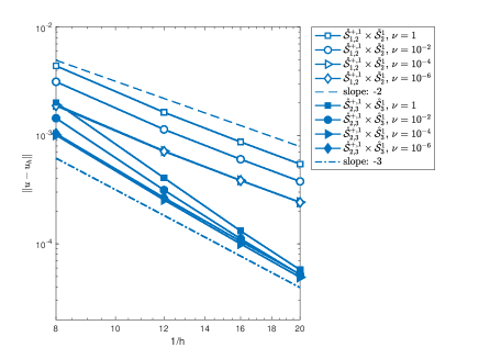
(a) The convergence rate of $\|\bm{u}-\bm{u}_{h}\|$.

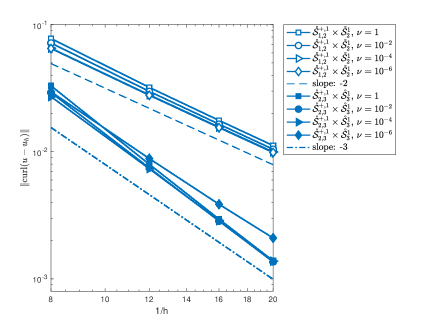
(b) The convergence rate of $\|\operatorname{curl}\bm{u}-\operatorname{curl}\bm{u}_{h}\|$.

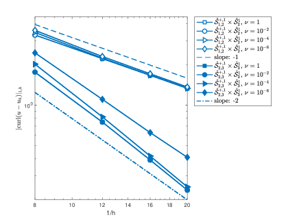
(c) The convergence rate of $|\operatorname{curl}\bm{u}-\operatorname{curl}\bm{u}_{h}|_{1,h}$.

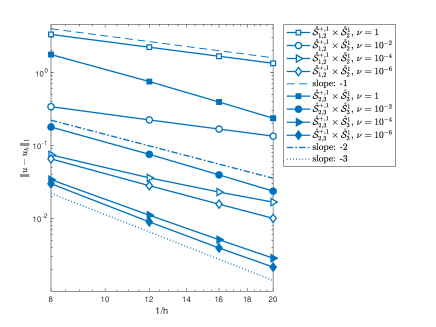
(d) The convergence rate of ${|||}\bm{u}-\bm{u}_{h}{|||}_{1}$.

Figure 6.1. Convergence rates for Example 1

Example 2.

We consider the Brinkman problem (1.2) with $\Omega=[0,1]\times[0,1]\times[0,1]$. Cut the unit cube into eight cubes and each of the eight cubes is refined into eight half-sized cubes uniformly to get a higher-level grid. The mesh size $h$ of each level is $1/2$, $1/4$, $1/8$, $1/16$, respectively.

We use the finite element space $\mathring{\mathcal{S}}_{r-1}^{+,2}\times\mathring{\mathcal{S}}_{r-2}^{3}$ with $r=2,3$ to discretize $(\bm{u};p)$ in (5.1). Let $\alpha=1$ in (1.2), and let the effective viscosity $\nu$ be $1$, $10^{-2}$, $10^{-4}$, and $10^{-6}$. We consider the system (1.2) with $g=0$ and $\bm{f}=-\operatorname{div}(\nu\operatorname{grad}\bm{u})+\alpha\bm{u}+\operatorname{grad}p$, where

$$\bm{u}=\operatorname{curl}\begin{pmatrix}y^{2}(1-y)^{2}x(1-x)z^{2}(1-z)^{3}\\ x^{2}(1-x)^{2}y(1-y)z^{2}(1-z)^{3}\\ 0\end{pmatrix},$$ (6.1)

and

$$p=\left(x-\frac{1}{2}\right)\left(y-\frac{1}{2}\right)(1-z).$$ (6.2)

For different values of $\nu$ and $h$, we present the errors of the velocity $\bm{u}_{h}$ measured in various norms and the errors of the pressure $p_{h}$ measured in the $L^{2}$ norm in Figure 6.2. It can be observed that the optimal order of convergence is achieved, and the discretization is stable as $\nu$ tends to 0. In particular, Figure 6.2c shows that ${|||}\bm{u}-\bm{u}_{h}{|||}_{2}$ has one-order higher convergence rate when $\nu$ is sufficiently small, which is in accordance with Remark 5.1.

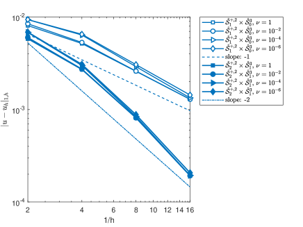
(a) The convergence rates of $|\bm{u}-\bm{u}_{h}|_{1,h}$.

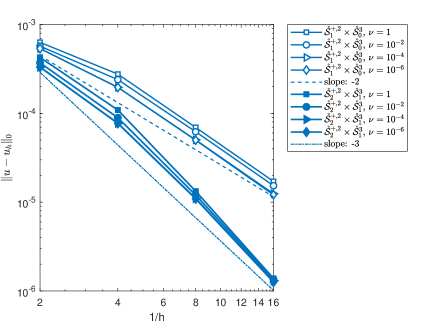
(b) The convergence rate of $\|\bm{u}-\bm{u}_{h}\|$.

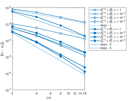
(c) The convergence rate of ${|||}\bm{u}-\bm{u}_{h}{|||}_{2}$.

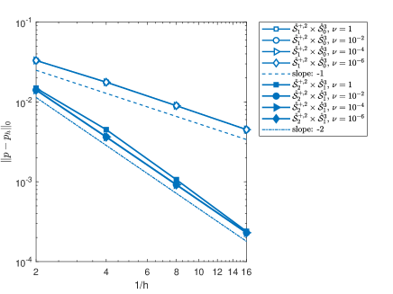
(d) The convergence rate of $\|p-p_{h}\|$.

Figure 6.2. Convergence rates for Example 2

7. Conclusion

In this paper, we constructed a family of $H(\operatorname{grad}\operatorname{curl})$-nonconforming elements for the $-\operatorname{curl}\Delta\operatorname{curl}$ problems and a family of uniformly stable $[H^{1}]^{3}$-nonconforming cubical elements for the Brinkman problem. The two families of elements can fit into a de Rham complex starting with the serendipity finite element space and ending with the piecewise polynomial space. Because of their $H(\operatorname{curl})$ and $H(\operatorname{div})$-conformity, they can also be applied to the Darcy problem and Maxwell equations even though this is not a focus of this paper.

The newly-proposed $H(\operatorname{grad}\operatorname{curl})$-nonconforming element has at least 48 DOFs on each element. To further reduce the number of DOFs, we will construct fully nonconforming elements in future works.

In this paper, we considered cubical elements, while it is not hard to extend this construction to rectangular meshes. In the future, we will extend the construction to general quadrilateral and hexahedral meshes.

References

- [1] D. N. Arnold and G. Awanou. The serendipity family of finite elements. Foundations of computational mathematics, 11(3):337–344, 2011.
- [2] D. N. Arnold and G. Awanou. Finite element differential forms on cubical meshes. Mathematics of Computation, 83(288):1551–1570, 2014.
- [3] D. N. Arnold, F. Brezzi, and M. Fortin. A stable finite element for the Stokes equations. Calcolo, 21(4):337–344, 1984.
- [4] D. N Arnold and J. Qin. Quadratic velocity/linear pressure Stokes elements. Advances in computer methods for partial differential equations, 7:28–34, 1992.
- [5] S. C. Brenner. Poincaré–Friedrichs inequalities for piecewise functions. SIAM Journal on Numerical Analysis, 41(1):306–324, 2003.
- [6] L. Chacón, A. N. Simakov, and A. Zocco. Steady-state properties of driven magnetic reconnection in 2D electron magnetohydrodynamics. Physical review letters, 99(23):235001, 2007.
- [7] S. Chen, L. Dong, and J. Zhao. Uniformly convergent cubic nonconforming element for Darcy–Stokes problem. Journal of Scientific Computing, 72(1):231–251, 2017.
- [8] S. H. Christiansen and K. Hu. Generalized finite element systems for smooth differential forms and Stokes’ problem. Numerische Mathematik, 140(2):327–371, 2018.
- [9] M. Crouzeix and P.-A. Raviart. Conforming and nonconforming finite element methods for solving the stationary Stokes equations I. Revue française d’automatique informatique recherche opérationnelle. Mathématique, 7(R3):33–75, 1973.
- [10] G. Fu, J. Guzmán, and M. Neilan. Exact smooth piecewise polynomial sequences on Alfeld splits. Mathematics of Computation, 89(323):1059–1091, 2020.
- [11] A. Gillette and T. Kloefkorn. Trimmed serendipity finite element differential forms. Mathematics of Computation, 88(316):583–606, 2019.
- [12] V. Girault and P. Raviart. Finite element methods for Navier-Stokes equations: theory and algorithms, volume 5. Springer Science & Business Media, 2012.
- [13] J. Guzmán and M. Neilan. A family of nonconforming elements for the brinkman problem. IMA Journal of Numerical Analysis, 32(4):1484–1508, 2012.
- [14] J. Guzmán and M. Neilan. Inf-sup stable finite elements on barycentric refinements producing divergence–free approximations in arbitrary dimensions. SIAM Journal on Numerical Analysis, 56(5):2826–2844, 2018.
- [15] J. Guzmán and L. Scott. The Scott-Vogelius finite elements revisited. Mathematics of Computation, 88(316):515–529, 2019.
- [16] Johnny Guzmán, Anna Lischke, and Michael Neilan. Exact sequences on worsey–farin splits. Mathematics of Computation, 91(338):2571–2608, 2022.
- [17] R. Hiptmair. Finite elements in computational electromagnetism. Acta Numerica, 11:237–339, 2002.
- [18] K. Hu, Q. Zhang, and Z. Zhang. Simple curl-curl-conforming finite elements in two dimensions. SIAM Journal on Scientific Computing, 42(6):A3859–A3877, 2020.
- [19] K. Hu, Q. Zhang, and Z. Zhang. Simple curl-curl-conforming finite elements in two dimensions (erratum). arXiv:2004.12507v2, 2020.
- [20] K. Hu, Q. Zhang, and Z. Zhang. A family of finite element stokes complexes in three dimensions. SIAM Journal on Numerical Analysis, 60(1):222–243, 2022.
- [21] Xuehai Huang. Nonconforming finite element stokes complexes in three dimensions. Science China Mathematics, pages 1–24, 2023.
- [22] K. A. Mardal, X. Tai, and R. Winther. A robust finite element method for Darcy–Stokes flow. SIAM Journal on Numerical Analysis, 40(5):1605–1631, 2002.
- [23] R. D. Mindlin and H. F. Tiersten. Effects of couple-stresses in linear elasticity. Archive for Rational Mechanics and Analysis, 11(1):415–448, 1962.
- [24] P. Monk. Finite Element Methods for Maxwell’s Equations. Oxford University Press, 2003.
- [25] M. Neilan. Discrete and conforming smooth de Rham complexes in three dimensions. Mathematics of Computation, 84(295):2059–2081, 2015.
- [26] M. Neilan and D. Sap. Stokes elements on cubic meshes yielding divergence-free approximations. Calcolo, 53(3):263–283, 2016.
- [27] S. K. Park and X. Gao. Variational formulation of a modified couple stress theory and its application to a simple shear problem. Zeitschrift für angewandte Mathematik und Physik, 59(5):904–917, 2008.
- [28] X. Tai and R. Winther. A discrete de Rham complex with enhanced smoothness. Calcolo, 43(4):287–306, 2006.
- [29] C. Taylor and P. Hood. A numerical solution of the Navier-Stokes equations using the finite element technique. Computers & Fluids, 1(1):73–100, 1973.
- [30] L. Wang, H. Li, and Z. Zhang. )-conforming spectral element method for quad-curl problems. Computational Methods in Applied Mathematics, 21(3):661–681, 2021.
- [31] L. Wang, W. Shan, H. Li, and Z. Zhang. )-conforming quadrilateral spectral element method for quad-curl problems. Mathematical Models and Methods in Applied Sciences, 31(10):1951–1986, 2021.
- [32] X. Xie, J. Xu, and G. Xue. Uniformly-stable finite element methods for Darcy-Stokes-Brinkman models. Journal of Computational Mathematics, pages 437–455, 2008.
- [33] X. Xu and S. Zhang. A new divergence-free interpolation operator with applications to the Darcy–Stokes–Brinkman equations. SIAM Journal on Scientific Computing, 32(2):855–874, 2010.
- [34] Q. Zhang, L. Wang, and Z. Zhang. )-conforming finite elements in 2 dimensions and applications to the quad-curl problem. SIAM Journal on Scientific Computing, 41(3):A1527–A1547, 2019.
- [35] Q. Zhang and Z. Zhang. A family of curl-curl conforming finite elements on tetrahedral meshes. CSIAM Transactions on Applied Mathematics, 1(4):639–663, 2020.
- [36] S. Zhang. A new family of stable mixed finite elements for the 3D Stokes equations. Mathematics of computation, 74(250):543–554, 2005.
- [37] S. Zhang. On the Powell-Sabin divergence-free finite element for the Stokes equations. Journal of Computational Mathematics, pages 456–470, 2008.
- [38] S. Zhang. A family of divergence-free finite elements on rectangular grids. SIAM journal on numerical analysis, 47(3):2090–2107, 2009.
- [39] S. Zhang. Quadratic divergence-free finite elements on Powell–Sabin tetrahedral grids. Calcolo, 48(3):211–244, 2011.
- [40] B. Zheng, Q. Hu, and J. Xu. A nonconforming finite element method for fourth order curl equations in . Mathematics of Computation, 80(276):1871–1886, 2011.
- [41] X. Zhou, Z. Meng, and J. Su. Low-order nonconforming brick elements for the 3D Brinkman model. Computers & Mathematics with Applications, 98:201–217, 2021.