Understanding Decision-Time vs. Background Planning in Model-Based Reinforcement Learning

Abstract

In model-based reinforcement learning, an agent can leverage a learned model to improve its way of behaving in different ways. Two prevalent approaches are decision-time planning and background planning. In this study, we are interested in understanding under what conditions and in which settings one of these two planning styles will perform better than the other in domains that require fast responses. After viewing them through the lens of dynamic programming, we first consider the classical instantiations of these planning styles and provide theoretical results and hypotheses on which one will perform better in the pure planning, planning & learning, and transfer learning settings. We then consider the modern instantiations of these planning styles and provide hypotheses on which one will perform better in the last two of the considered settings. Lastly, we perform several illustrative experiments to empirically validate both our theoretical results and hypotheses. Overall, our findings suggest that even though decision-time planning does not perform as well as background planning in their classical instantiations, in their modern instantiations, it can perform on par or better than background planning in both the planning & learning and transfer learning settings.

1 Introduction

It has long been argued that, in order for reinforcement learning (RL) agents to adapt to a variety of changing tasks, they should be able to learn a model of their environment, which allows for counterfactual reasoning and fast re-planning [18]. Although this is a widely-accepted view in the RL community, the question of how to leverage a learned model to perform planning in the first place does not have a widely-accepted and clear answer. In model-based RL, the two prevalent planning styles are decision-time (DT) and background (B) planning [24], where the agent mainly plans in the moment and in parallel to its interaction with the environment, respectively. Even though these two planning styles have been developed with different assumptions and application domains in mind, i.e., DT planning algorithms [27, 28, 20, 21] under the assumption that the exact model of the environment is known and for domains that allow for certain computational budgets, such as board games, and B planning algorithms [22, 23, 33, 13] under the assumption that the exact model is unknown and for domains that usually require fast responses, such as basic gridworlds and video games, recently, with the introduction of the ability to learn a model through pure interaction [19], DT planning algorithms have been applied to the same domains as their B planning counterparts (see e.g., [19, 14]). However, it still remains unclear under what conditions and in which settings one of these planning styles will perform better than the other in these fast-response-requiring domains.

To clarify this, we first start by abstracting away from the specific implementation details of the two planning styles and view them in a unified way through the lens of dynamic programming (DP). Then, we consider the classical instantiations (CI) of these planning styles and based on their DP interpretations, provide theoretical results and hypothesis on which one will perform better in the pure planning (PP), planning & learning (P&L), and transfer learning (TL) settings. We then consider the modern instantiations (MI) of these two planning styles and based on both their DP interpretations and implementation details, provide hypotheses on which one will perform better in the P&L and TL settings. Lastly, we perform illustrative experiments with both instantiations of these planning styles to empirically validate our theoretical results and hypotheses. Overall, our results suggest that even though DT planning does not perform as well as B planning in their CIs, due to (i) the improvements in the way planning is performed, (ii) the usage of only real experience in the updates of the value estimates, and (iii) the ability to improve upon the previously obtained policy at test time, the MIs of it can perform on par or better than their B planning counterparts in both the P&L and TL settings. We hope that our findings will help the RL community in developing a better understanding of the two planning styles and stimulate research in improving of them in potentially interesting ways.

2 Background

In value-based RL [24], an agent $A$ interacts with its environment $E$ through a sequence of actions to maximize its long-term cumulative reward. Here, the environment is usually modeled as a Markov decision process $E=(\mathcal{S}_{E},\mathcal{A}_{E},p_{E},r_{E},d_{E},\gamma)$, where $\mathcal{S}_{E}$ and $\mathcal{A}_{E}$ are the (finite) set of states and actions, $p_{E}:\mathcal{S}_{E}\times\mathcal{A}_{E}\times\mathcal{S}_{E}\to[0,1]$ is the transition distribution, $r_{E}:\mathcal{S}_{E}\times\mathcal{A}_{E}\times\mathcal{S}_{E}\to\amsmathbb{R}$ is the reward function, $d_{E}:\mathcal{S}_{E}\to[0,1]$ is the initial state distribution, and $\gamma\in[0,1)$ is the discount factor. At each time step $t$, after taking an action $a_{t}\in\mathcal{A}_{E}$, the environment’s state transitions from $s_{t}\in\mathcal{S}_{E}$ to $s_{t+1}\in\mathcal{S}_{E}$, and the agent receives an observation $o_{t+1}\in\mathcal{O}_{E}$ and an immediate reward $r_{t}$. We assume that the observations are generated by a deterministic procedure $\psi:\mathcal{S}_{E}\to\mathcal{O}_{E}$, unknown to the agent. As the agent usually does not have access to the states in $\mathcal{S}_{E}$ a priori, and as the observations in $\mathcal{O}_{E}$ are usually very high-dimensional, it has to operate on its own state space $\mathcal{S}_{A}$, which is generated by its own adaptable (or sometimes a priori fixed) value encoder $\phi:\mathcal{O}_{E}\to\mathcal{S}_{A}$. The goal of the agent is to jointly learn a value encoder $\phi$ and a value estimator (VE) $Q:\mathcal{S}_{A}\times\mathcal{A}_{E}\to\amsmathbb{R}$ that induces a policy $\pi:\mathcal{S}_{A}\times\mathcal{A}_{E}\to[0,1]\in\mathbb{\Pi}$, where $\mathbb{\Pi}\equiv\{\pi|\pi:\mathcal{S}_{A}\times\mathcal{A}_{E}\to[0,1]\}$, maximizing $E_{\pi,p_{E}}[\sum_{t=0}^{\infty}\gamma^{t}r_{E}(S_{t},A_{t},S_{t+1})|S_{0}\sim d_{E}]$. For convenience, we will refer to the composition of $\phi$ and $Q$ as simply the VE.

Model-Free & Model-Based RL. The two main ways of achieving this goal are through the use of model-free RL (MFRL) and model-based RL (MBRL) methods. In MFRL, there is just a learning phase and the gathered experience is mainly used in improving the VE. In MBRL, there are two alternating phases: the learning and planning phases. In the learning phase, in contrast to MFRL, the gathered experience is mainly used in jointly learning an adaptable (or sometimes a priori fixed) model encoder $\varphi:\mathcal{O}_{E}\to\mathcal{S}_{M}$ and a model $m\equiv(p_{M},r_{M},d_{M})\in\mathcal{M}$, where $\mathcal{M}\equiv\{(p_{M},r_{M},d_{M})|p_{M}:\mathcal{S}_{M}\times\mathcal{A}_{E}\times\mathcal{S}_{M}\to[0,1],r_{M}:\mathcal{S}_{M}\times\mathcal{A}_{E}\times\mathcal{S}_{M}\to\amsmathbb{R},d_{M}:\mathcal{S}_{M}\to[0,1]\}$ and $\mathcal{S}_{M}$ is the state space of the agent’s model, and optionally, as in MFRL, the experience may also be used in improving the VE. Again, for convenience, we will refer to the composition of $\varphi$ and $m$ as simply the model. In the planning phase, the learned model $m$ is then used for simulating experience, either to be used alongside real experience in improving the VE, or just to be used in selecting actions at decision time. Note that in general $\varphi\neq\phi$ and thus $\mathcal{S}_{M}\neq\mathcal{S}_{A}$. However, in these cases, we assume that the agent has access to a deterministic function $\rho:\mathcal{S}_{M}\to\mathcal{S}_{A}$ that allows for going from $\mathcal{S}_{M}$ to $\mathcal{S}_{A}$. We also assume that $\mathcal{S}_{E}\subseteq\mathcal{S}_{M}$, which implies that the agent’s model is, in principle, capable of exactly modeling the environment, though this may be very hard in practice.

Planning Styles in MBRL. In MBRL, planning is performed in two different styles: (i) DT planning, and (ii) B planning (see Ch. 8 of [24]). DT planning, also known as “planning in the now”, is performed as a computation whose output is the selection of a single action for the current state. This is often done by unrolling the model forward from the current state to compute local value estimates, which are then usually discarded after action selection. Here, planning is performed independently for every encountered state and it is mainly performed in an online fashion, though it may also contain offline components. In contrast, B planning is performed by continually improving a cached VE, on the basis of simulated experience from the model, often in a global manner. Action selection is then quickly done by querying the VE at the current state. Unlike DT planning, B planning is often performed in a purely offline fashion, in parallel to the agent-environment interaction, and thus is not necessarily focused on the current state: well before action selection for any state, planning plays its part in improving the value estimates in many other states. For convenience, in this study, we will refer to all MBRL algorithms that have an online planning component as DT planning algorithms (see e.g., [27, 28, 20, 21, 19, 32]), and will refer to the rest as B planning algorithms (see e.g., [22, 23, 33, 13, 32]). Note that, regardless of the style, any type of planning can be viewed as a procedure $f:(\mathcal{M},\mathbb{\Pi})\to\mathbb{\Pi}$ that takes a model $m$ and a policy $\pi^{i}$ as input and returns an improved policy $\pi_{m}^{o}$, according to $m$, as output.

Algorithms within the Two Planning Styles. Starting with DT planning, depending on how much search is performed, DT planning algorithms can be studied under three main categories: DT planning algorithms (i) that perform no search (see e.g., [28] and Alg. 1), (ii) that perform pure search (see e.g., [9] and Alg. 2), and (iii) that perform some amount of search (see e.g., [20, 21, 19] and Alg. 5). In the first two, planning is performed by just running pure rollouts with a fixed or improving policy (see Fig. 1(a)), and by purely performing search (see Fig. 1(b)), respectively. In the last one, planning is performed by first performing some amount of search and then either by running rollouts with a fixed or improving policy, by bootstrapping on the cached value estimates of a fixed or improving policy, or by doing both (see Fig. 1(c) & 1(d)). Note that while the CIs of DT planning fall within the first two categories, the MIs of it usually fall within the last one. Also note that, while planning is performed with only a single parametric model in the first two categories, it is usually performed with both a parametric and non-parametric (usually a replay buffer, see [29]) model in the last one (see e.g., [19] and Alg. 5). See [7] for more details on the different categories of DT planning. Moving on to B planning, as all B planning algorithms (see e.g., Alg. 3, 4, 6) perform planning by periodically improving a cached VE throughout the model learning process, we do not study them under different categories. However, we again note that, while some B planning algorithms perform planning with a single parametric model (see e.g., Alg. 3 & 4), some perform planning with both a parametric and non-parametric (again usually a replay buffer) model (see e.g., Alg. 6).

3 A Unified View of the Two Planning Styles

In this section, we abstract away from the specific implementation details, such as whether policy improvement is done locally or globally, or whether planning is performed in an online or offline manner, and view the two planning styles in a unified way through the lens of DP [8]. More specifically, we view DT planning through the lens of policy iteration (PI) as DT planning algorithms can be considered as performing some amount of asynchronous PI that is focused on the current state (see [7]), and we view B planning through the lens of value iteration (VI) as B planning algorithms can be considered as performing some amount of asynchronous VI that is focused on the sampled states (see [24]).

In this framework, DT planning algorithms that perform no search can be considered as performing one-step PI at every encountered state, on top of a fixed or improving policy, as they compute $\pi_{m}^{o}$ by first running many rollouts with a fixed or improving $\pi^{i}$ in $m$ to evaluate the current state, and then by selecting the most promising action (which can be considered as first performing policy evaluation and then policy improvement). Similarly, DT planning algorithms that perform pure search can be considered as performing PI until convergence (which we call full PI) at every encountered state as they disregard $\pi^{i}$ and compute $\pi_{m}^{o}$ by first performing exhaustive search in $m$ to obtain the optimal values at the current state, and then by selecting the most promising action. Finally, DT planning algorithms that perform some amount of search can be considered as performing something between one-step and full PI at every encountered state, on top of a fixed or improving policy, as they are just a mixture of DT planning algorithms that perform no search and pure search. Hence, depending on how much search is performed, DT planning algorithms in general can be viewed as going between the spectrum of performing one-step PI and full PI at every encountered state, on top of a fixed or improving policy.

Similarly, under the assumption that all states are sampled at least once during planning, all B planning algorithms can also be considered as performing either one-step VI, VI until convergence (which we call full VI), or something in between, on top of a fixed or improving policy, as they compute $\pi_{m}^{o}$ by periodically improving a fixed or improving $\pi^{i}$ on the basis of simulated experience from $m$, either for a single time step, until convergence, or somewhere in between. Thus, depending on much planning is performed, B planning algorithms in general can also be viewed as interpolating between performing one-step VI and full VI, on top of a fixed or improving policy.

Finally, note that, in Sec. 2, we have pointed out that some DT and B planning algorithms perform planning with both a parametric and non-parametric model, which can make it hard for them to be viewed through our proposed framework. However, if one considers the two separate models as a single combined model, then these algorithms can also be viewed straightforwardly in our proposed framework: DT and B planning algorithms that perform planning with two separate models can still be viewed as going between the spectrum of performing one-step PI / VI and full PI / VI, however now, they would just be performing planning with a combined model (see App. F for a broader discussion on the combined model view).

4 Decision-Time vs. Background Planning

In this study, we are interested in understanding under what conditions and in which settings one planning style will perform better than the other. Thus, we start by defining a performance measure that will be used in comparing the two planning styles of interest. Given an arbitrary model $m=(p,r,d)\in\mathcal{M}$, let us define the performance of an arbitrary policy $\pi\in\mathbb{\Pi}$ in it as follows:

$$J_{m}^{\pi}\equiv E_{\pi,p}[{\textstyle\sum}_{t=0}^{\infty}\gamma^{t}r(S_{t},A_{t},S_{t+1})|S_{0}\sim d].$$ (1)

Note that $J_{m}^{\pi}$ corresponds to the expected discounted return of a policy $\pi$ in model $m$. Next, we consider the conditions under which the comparisons will be made: we are interested in both simple scenarios in which the VEs and models are both represented as a table, and in complex ones in which at least the VEs or models are represented using function approximation (FA).

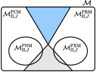
(a) General partitioning

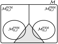
(b) Partitioning of interest

Figure 1: (a) The general partitioning and (b) the partitioning of interest of $\mathcal{M}$, for a given $\Pi$ and $J$. The gray and blue regions indicate $\mathcal{M}_{\Pi,J}^{\textnormal{PCM}}\cap\mathcal{M}_{\Pi,J}^{\textnormal{PRM}}$ and $\mathcal{M}\setminus(\mathcal{M}_{\Pi,J}^{\textnormal{PCM}}\cup\mathcal{M}_{\Pi,J}^{\textnormal{PRM}})$, respectively.

Partitioning of the Model Space. We now present a way to partition the space of agent models $\mathcal{M}$ such that one planning style is guaranteed to perform on par or better than the other. Let us start by defining $m^{*}$ to be the exact model of the environment. Note that $m^{*}\in\mathcal{M}$, as we assumed that $\mathcal{S}_{E}\subseteq\mathcal{S}_{M}$ (see Sec. 2). Then, given a policy set $\Pi\subseteq\mathbb{\Pi}$, containing at least two policies, and a performance measure $J$, defined as in (1), depending on the relative performances of the policies in it and in $m^{*}$, a model $m\in\mathcal{M}$ can belong to one of the following main classes:

Definition 1 (PCM).

Given $\Pi\subseteq\mathbb{\Pi}$ and $J$, let $\mathcal{M}_{\Pi,J}^{\textnormal{PCM}}\equiv\{m\in\mathcal{M}\ |\ \smash{J_{m^{*}}^{\pi^{i}}\lesseqgtr J_{m^{*}}^{\pi^{j}}}\ \forall\pi^{i},\pi^{j}\in\Pi\text{ satisfying }\smash{J_{m}^{\pi^{i}}\gtreqless J_{m}^{\pi^{j}}}\}$. We say that each $m\in\mathcal{M}_{\Pi,J}^{\textnormal{PCM}}$ is a performance-contrasting model (PCM) of $m^{*}$ w.r.t. $\Pi$ and $J$.

Definition 2 (PRM).

Given $\Pi\subseteq\mathbb{\Pi}$ and $J$, let $\mathcal{M}_{\Pi,J}^{\textnormal{PRM}}\equiv\{m\in\mathcal{M}\ |\ \smash{J_{m^{*}}^{\pi^{i}}\gtreqless J_{m^{*}}^{\pi^{j}}}\ \forall\pi^{i},\pi^{j}\in\Pi\text{ satisfying }\smash{J_{m}^{\pi^{i}}\gtreqless J_{m}^{\pi^{j}}}\}$. We say that each $m\in\mathcal{M}_{\Pi,J}^{\textnormal{PRM}}$ is a performance-resembling model (PRM) of $m^{*}$ w.r.t. $\Pi$ and $J$.

Informally, given any two policies in $\Pi$, and $J$, a model $m$ is a PCM of $m^{*}$ iff the policy that performs on par or better in it performs on par or worse in $m^{*}$, and it is a PRM of $m^{*}$ iff the policy that performs on par or better in it also performs on par or better in $m^{*}$. Note that $m$ can both be a PCM and a PRM of $m^{*}$ iff the two policies perform on par in both $m$ and $m^{*}$. If $\Pi$ contains at least one of the optimal policies for $m$, then $m$ can also belong to one of the following specialized classes:

Definition 3 (PNM).

Given $\Pi\subseteq\mathbb{\Pi}$ and $J$, let $\mathcal{M}_{\Pi,J}^{\textnormal{PNM}}\equiv\{m\in\mathcal{M}_{\Pi,J}^{\textnormal{PCM}}\ |\ \smash{J_{m^{*}}^{\pi_{m}^{*}}=\min_{\pi\in\mathbb{\Pi}}J_{m^{*}}^{\pi}}\ \forall\pi_{m}^{*}\in\Pi\}$, where $\pi_{m}^{*}$ denotes the optimal policies in $m$. We say that each $m\in\mathcal{M}_{\Pi,J}^{\textnormal{PNM}}$ is a performance-minimizing model (PNM) of $m^{*}$ w.r.t. $\Pi$ and $J$.

Definition 4 (PXM).

Given $\Pi\subseteq\mathbb{\Pi}$ and $J$, let $\mathcal{M}_{\Pi,J}^{\textnormal{PXM}}=\{m\in\mathcal{M}_{\Pi,J}^{\textnormal{PRM}}\ |\ \smash{J_{m^{*}}^{\pi_{m}^{*}}=\max_{\pi\in\mathbb{\Pi}}J_{m^{*}}^{\pi}}\ \forall\pi_{m}^{*}\in\Pi\}$, where $\pi_{m}^{*}$ denotes the optimal policies in $m$. We say that each $m\in\mathcal{M}_{\Pi,J}^{\textnormal{PXM}}$ is a performance-maximizing model (PXM) of $m^{*}$ w.r.t. $\Pi$ and $J$.

Informally, given a subset of $\Pi$ that contains the optimal policies for a model $m$, and $J$, $m$ is a PNM of $m^{*}$ iff all of the optimal policies result in the worst possible performance in $m^{*}$, and it is a PXM of $m^{*}$ iff all them result in the best possible performance in $m^{*}$. Note that all definitions above are agnostic to how the models are represented.

Fig. 1(a) illustrates how $\mathcal{M}$ is partitioned for a given $\Pi$ and $J$. Note that for a fixed $J$, the relative sizes of the model classes solely depend on $\Pi$. For instance, as $\Pi$ gets larger, the relative sizes of $\mathcal{M}_{\Pi,J}^{\textnormal{PCM}}$ and $\mathcal{M}_{\Pi,J}^{\textnormal{PRM}}$ shrink, because with every policy that is added to $\Pi$, the number of criteria that a model must satisfy to be a PCM or PRM increases, which reduces the odds of an arbitrary model in $\mathcal{M}$ being in $\mathcal{M}_{\Pi,J}^{\textnormal{PCM}}$ or $\mathcal{M}_{\Pi,J}^{\textnormal{PRM}}$. And, as $\Pi$ gets smaller, the relative sizes of $\mathcal{M}_{\Pi,J}^{\textnormal{PCM}}$ and $\mathcal{M}_{\Pi,J}^{\textnormal{PRM}}$ grow, and eventually fill up the entire space, when $\Pi$ contains only two policies. Fig. 1(b) illustrates the partitioning in this scenario. Since we are only interested in comparing the policies of two planning styles, the $\Pi$ of interest has a size of two, and thus we have a partitioning as in Fig. 1(b).

4.1 Classical Instantiations of the Two Planning Styles

We are now ready to discuss when will one planning style perform better than the other. For easy analysis, we start by considering the CIs of the two planning styles in which both the VEs and models are represented as a table. More specifically, for DT planning we study a version of the OMCP algorithm of Tesauro and Galperin [28] in which a parametric model is learned from experience (see Alg. 1), and for B planning we study a simplified version of the Dyna-Q algorithm of Sutton [22, 23] in which planning is performed until convergence with every model in the model learning process (see Alg. 4). See App. B for a discussion on why we consider these versions. Note that these two algorithms can be considered as performing one-step PI and full VI on top of a fixed policy, respectively (see Sec. 3). Also note that, although we only consider these specific instantiations, as long as the VEs of both planning styles are represented as a table and DT planning corresponds to taking a smaller or on par policy improvement step than B planning, which is the case in most CIs, the results that we derive in this section would hold regardless of the choice of instantiation. Before considering different settings, let us define the following policies that will be useful in referring to the input and output policies of the two planning styles:

Definition 5 (Base, Rollout [7] & CE [16] Policies).

The base policy $\pi^{b}\in\mathbb{\Pi}$ is the policy used in initiating PI or VI. Given a fixed or improving base policy $\pi^{b}$ and a model $m\in\mathcal{M}$, the rollout policy $\pi_{m}^{r}\in\mathbb{\Pi}$ is the policy obtained after performing one-step of PI on top of $\pi^{b}$ in $m$, and the certainty-equivalence (CE) policy $\pi_{m}^{ce}\in\mathbb{\Pi}$ is the policy obtained after performing full PI or full VI on top of $\pi^{b}$ in $m$.

In the rest of this section, we will refer to the policies generated by the CIs of DT and B planning with model $m$ on top of a fixed base policy $\pi^{b}$ as $\pi_{m}^{r}$ and $\pi_{m}^{ce}$, respectively.

PP Setting. We start by considering the PP setting in which the agent is directly provided with a model. In this setting, we can prove the following statements:

Proposition 1.

Let $m\in\mathcal{M}$ be a PCM of $m^{*}$ w.r.t. $\Pi=\{\pi_{m}^{r},\pi_{m}^{ce}\}\subseteq\mathbb{\Pi}$ and $J$. Then, $J_{m^{*}}^{\pi_{m}^{r}}\geq J_{m^{*}}^{\pi_{m}^{ce}}$.

Proposition 2.

Let $m\in\mathcal{M}$ be a PRM of $m^{*}$ w.r.t. $\Pi=\{\pi_{m}^{r},\pi_{m}^{ce}\}\subseteq\mathbb{\Pi}$ and $J$. Then, $J_{m^{*}}^{\pi_{m}^{ce}}\geq J_{m^{*}}^{\pi_{m}^{r}}$.

Due to space constraints, we defer all the proofs to App. C. Prop. 1 & 2 imply that, given $\Pi=\{\pi_{m}^{r},\pi_{m}^{ce}\}$ and $J$, although DT planning will perform on par or better than B planning when the provided model $m$ is a PCM, it will perform on par or worse when $m$ is a PRM. Note that these results would not be guaranteed to hold if FA was introduced in the VE representations, as in this case, there would be no guarantee that full VI will result in a better policy than one-step PI in $m$ [8]. However, if one were to use approximators with good generalization capabilities (GGC), i.e., approximators that assign the same value to similar observations, we would expect a similar performance trend to hold.

P&L Setting. In the P&L setting, instead of being provided directly, the model has to be learned from the experience gathered by the agent. In this scenario, as different policies are likely to be used in the model learning process, the encountered models of the two planning styles, which we denote as $\bar{m}\in\mathcal{M}$ and $\bar{\bar{m}}\in\mathcal{M}$ for DT and B planning, respectively, are also likely to be different. Thus, as they require the two planning styles to have access to the same model, the results of Prop. 1 & 2 are not valid in the P&L setting. However, if the model of B planning is a PNM or a PXM, we can prove the following statements:

Proposition 3.

Let $\bar{m}\in\mathcal{M}$ be a PCM or a PRM of $m^{*}$ w.r.t. $\bar{\Pi}=\{\pi_{\bar{m}}^{r},\pi_{\bar{m}}^{ce}\}\subseteq\mathbb{\Pi}$ and $J$, and let $\bar{\bar{m}}\in\mathcal{M}$ be a PNM of $m^{*}$ w.r.t. $\bar{\bar{\Pi}}=\{\pi_{\bar{\bar{m}}}^{r},\pi_{\bar{\bar{m}}}^{ce}\}\subseteq\mathbb{\Pi}$ and $J$. Then, $J_{m^{*}}^{\pi_{\bar{m}}^{r}}\geq J_{m^{*}}^{\pi_{\bar{\bar{m}}}^{ce}}$.

Proposition 4.

Let $\bar{m}\in\mathcal{M}$ be a PCM or a PRM of $m^{*}$ w.r.t. $\bar{\Pi}=\{\pi_{\bar{m}}^{r},\pi_{\bar{m}}^{ce}\}\subseteq\mathbb{\Pi}$ and $J$, and let $\bar{\bar{m}}\in\mathcal{M}$ be a PXM of $m^{*}$ w.r.t. $\bar{\bar{\Pi}}=\{\pi_{\bar{\bar{m}}}^{r},\pi_{\bar{\bar{m}}}^{ce}\}\subseteq\mathbb{\Pi}$ and $J$. Then, $J_{m^{*}}^{\pi_{\bar{\bar{m}}}^{ce}}\geq J_{m^{*}}^{\pi_{\bar{m}}^{r}}$.

Prop. 3 & 4 imply that, given $\bar{\Pi}=\{\pi_{\bar{m}}^{r},\pi_{\bar{m}}^{ce}\}$, $\bar{\bar{\Pi}}=\{\pi_{\bar{\bar{m}}}^{r},\pi_{\bar{\bar{m}}}^{ce}\}$ and $J$, although DT planning will perform on par or better than B planning when $\bar{\bar{m}}$ is a PNM, it will perform on par or worse when $\bar{\bar{m}}$ is a PXM. While the former result can be relevant in the initial phases of B planning’s model learning process, the latter one is most likely to be relevant in the final phases of this process, when $\bar{\bar{m}}$ becomes a PXM. Note that since the models are represented as tables, the learned models of both planning styles are guaranteed to become PXMs in the limit, as we know that in the worst case, with sufficient exploration, the models will, in the limit, converge to $m^{*}$ [24]. However, note that this would not be guaranteed if FA was used in the model representations. Lastly, even if $\bar{\bar{m}}$ starts as a PNM and eventually becomes a PXM, the results of Prop. 3 & 4 would not be guaranteed to hold if FA was used in the VE representations, due to the reason discussed in the PP setting. However, if one were to use approximators with GGC, we would again expect a similar performance trend to hold.

TL Setting. Although there are many different settings in TL [26], for easy analysis, we start by considering the simplest one in which there is only one training task (TRT) and one subsequent test task (TST), differing only in their reward functions, and in which the agent’s transfer ability is measured by how fast it adapts to the TST after being trained on the TRT (more challenging settings will be considered in the next section). In this setting, we would expect the results of the P&L setting to hold directly, as instead of a single one, there are now two consecutive P&L settings.

4.2 Modern Instantiations of the Two Planning Styles

We now consider the MIs of the two planning styles in which both the VEs and models are represented with neural networks (NN). More specifically, we study the DT and B planning algorithms in Zhao et al. [32] (see Alg. 5 & 6) as they are reflective of many of the properties of their state-of-the-art counterparts (see e.g., [19, 33, 13]) and their code is publicly available. See App. E for a broader discussion on why we choose these algorithms. Here, as the DT planning algorithm performs planning by first performing some amount of search with a parametric model and then by bootstrapping on the value estimates of a continually improving policy, it can be considered as performing more than one-step PI on top of an improving policy in a combined model $\bar{m}_{c}$ (see Sec. 3). And, as the B planning algorithm performs planning by continually improving a VE at every time step with both a parametric and non-parametric (a replay buffer) model, it can be viewed as performing something between one-step VI and full VI on top of an improving policy with a combined model $\bar{\bar{m}}_{c}$ (see Sec. 3). However, if $\bar{\bar{m}}_{c}$ converges, it can be viewed as performing full VI, as in this case the continual improvements to the VE with the converged $\bar{\bar{m}}_{c}$ would eventually lead to an improvement that is equivalent to performing full VI. Note that although we only consider these specific instantiations, the hypotheses we provide in this section are generally applicable to most state-of-the-art MBRL algorithms, as the algorithms in [32] are reflective of many of their properties (see App. E).

P&L Setting. We start with the P&L setting, and skip the PP one as it is not a relevant setting used with the MIs. To ease the analysis, let us start by considering a simplified scenario in which both the VEs and models of the MIs of the two planning styles are represented as a table. Let us also define the improved rollout policy to be the policy $\pi_{m}^{r+}\in\mathbb{\Pi}$ obtained after performing more than one-step PI, with the exact number not being important, on top of a base policy $\pi^{b}\in\mathbb{\Pi}$ in model $m$, and let us also refer to the policies generated by the MIs of DT and B planning with models $\bar{m}_{c}$ and $\bar{\bar{m}}_{c}$ on top of an improving base policy $\pi^{b}$ as $\pi_{\bar{m}_{c}}^{r+}$ and $\pi_{\bar{\bar{m}}_{c}}^{ce}$, respectively. Then, using $\pi_{\bar{m}_{c}}^{r+}$ and $\pi_{\bar{\bar{m}}_{c}}^{ce}$ in place of $\pi_{\bar{m}}^{r}$ and $\pi_{\bar{\bar{m}}}^{ce}$, respectively, and under the assumption that $\bar{\bar{m}}_{c}$ converges, we would expect the formal statements of the P&L setting of Sec. 4.1 to hold exactly as DT planning still corresponds taking a smaller or on par policy improvement step than B planning. However, as DT planning now corresponds to performing more than one-step PI, we would expect the performance gap between the two planning styles to reduce in their MIs. Moreover, we would expect this gap to gradually close if both $\bar{m}_{c}$ and $\bar{\bar{m}}_{c}$ become, and remain as, PXMs, as the use of an improving policy for DT planning would result in a continually improving performance that gets closer to the one of B planning.

Coming back to our original scenario in which both the VEs and models of the MIs of the two planning styles are represented with NNs, we would expect a similar performance trend to hold as NNs are approximators that have GGC. However, this expectation is solely based on the DP interpretations of the two planning styles and thus does not take into account the implementation details of them, which can also play an important role on how the two planning styles will perform against each other in their MIs. Thus, in the following paragraph, we will discuss the impacts of the implementation details of the two planning styles on their learning speed and final performance, and based on this, will provide hypotheses on which planning style will perform better than the other.

In their MIs, both planning styles perform planning by unrolling NN-based parametric models which are known to easily lead to compounding model errors (CME, [25]). Thus, obtaining combined models that are PXMs becomes quite difficult, if not impossible, for both planning styles. Even though this problem can significantly be mitigated for both of them by unrolling the models for only a few time steps and then bootstrapping on the VEs for the rest, B planning can also suffer from updating its VE with the potentially harmful simulated experience generated by its NN-based parametric model (see e.g., [29, 15]), which can slowdown, or even prevent, it in reaching optimal (or close to optimal) performance. Note that this is not a problem in DT planning as its VE is only updated with real experience. Thus, based on these observations, we hypothesize that compared to DT planning, it is likely for B planning to suffer more in reaching optimal (or close to optimal) performance in their MIs.

TL Setting. We now consider two common TL settings that are both more challenging than the TL setting in Sec. 4.1. In these settings, there is a distribution of TRTs and TSTs, differing only in their observations. In the first one, the agent’s transfer ability is measured by how fast it adapts to the TSTs after being trained on the TRTs (see e.g., [30]), and in the second one, this ability is measured by its instantaneous performance on the TSTs as it gets trained on the TRTs, also known as “zero-shot transfer” in the literature (see e.g., [32, 2]). In these two settings, the implementation details of the two planning styles also play an important role on how they will perform against each other. Thus, in the following paragraph, we will also provide hypotheses based on these details.

In both TL settings, we would again expect B planning to suffer more in reaching the optimal (or close to optimal) performance on the TRTs because of the reasons discussed in the P&L setting. Additionally, in the first setting, after the tasks switch from the TRTs to the TSTs, we would expect B planning to suffer more in the adaptation process, as its parametric model, learned on the TRTs, would keep generating experience that resembles the TRTs until it adapts to the TSTs, which in the meantime can lead to harmful updates to its VE. Also, in the second setting, if the learned parametric model of DT planning is capable of simulating at least a few time steps of the TSTs, and if the learned policies of the both planning styles perform similarly on the TSTs, we would expect DT planning to perform better on the TSTs, as at test time, it would be able to improve upon the policy obtained during training by performing online planning. Note that, this is not possible for B planning, as it performs planning in an offline fashion and thus requires additional interaction with the TSTs to improve upon the policy obtained during training.

5 Experiments

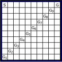
(a) SG Environment

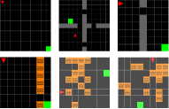
(b) MiniGrid Environments

Figure 2: (a) The SG environment and (b) MG environments: (top row) Empty 10x10, FourRooms, SCS9N1, (bottom row) LCS9N1, RDS Train, RDS Test.

We now perform illustrative experiments to validate the formal statements and hypotheses presented in Sec. 4. The experimental details and more detailed results can be found in App. G & H, respectively.

Environments. We perform experiments on both the Simple Gridworld (SG) environment and on environments that either pre-exist in or are manually built on top of MiniGrid (MG, [10]) (see Fig. 2), as the optimal policies in these environments are easy to learn and they allow for designing controlled experiments that are helpful in answering the questions of interest to this study. In the SG environment, the agent spawns in state S and has to navigate to the goal state depicted by G. In the MG environments, the agent, depicted in red, has to navigate to the green goal cell, while avoiding the orange lava cells (if there are any). More details on these environments can be found in App. G. Note that while $\mathcal{O}_{E}=\mathcal{S}_{E}$ in the SG environment, $\mathcal{O}_{E}\neq\mathcal{S}_{E}$ in the MG environments.

5.1 Experiments with Classical Instantiations

In this section, we perform experiments with the CIs of DT and B planning (see Alg. 1 & 4) on the SG environment to empirically validate our theoretical results and hypotheses in Sec. 4.1. In addition to the scenario in which both the VEs and models are represented as tables (where $\phi=\varphi$ are both identity functions (IF), implying $\mathcal{S}_{A}=\mathcal{S}_{M}=\mathcal{O}_{E}$), we also consider the one in which only the model is represented as a table (where only $\varphi$ is an IF, implying $\mathcal{S}_{M}=\mathcal{O}_{E}$). In the latter scenario, we use state aggregation (SA) in the VE representation, i.e., $\phi$ is a state aggregator, which allows for assigning the same value to similar observations. More on the implementation details of these NIs can be found in App. G.1.

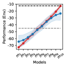
(a) Tabular

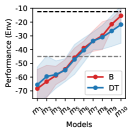
(b) State Aggregation

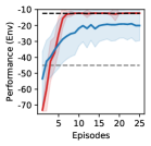
(c) Tabular

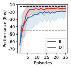
(d) State Aggregation

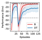
(e) Tabular

Figure 3: The performance of the CIs of DT and B planning on the SG environment, in the (a, b) PP, (c, d) P&L, and (e) TL settings with tabular and SA VE representations. Black & gray dashed lines indicate the performance of the optimal & random policies, respectively. Shaded regions are one standard error over 100 runs.

PP Experiments. According to Prop. 1 & 2, although DT planning is guaranteed to perform on par or better than B planning when the provided model is a PCM, it is guaranteed to perform on par or worse when the provided model is a PRM. To empirically verify this, we provided the two planning styles with a series of hand-designed tabular models that interpolate between a PNM and a PXM: the provided models first start with the PNM $m_{1}$ with goal state G₁ (see Fig. 2(a)), and then gradually move towards the PXM $m_{10}$ with goal state G, by first becoming PCMs $\{m_{i}\}_{i=2}^{5}$, and then by becoming PRMs $\{m_{j}\}_{j=6}^{9}$, with goal states $\{\text{G}_{n}\}_{n=2}^{9}$, respectively (see App. G.1 for more details on these models). After planning was performed with each of these models, we evaluated the resulting output policies in the environment. Results are shown in Fig. 3(a). We can indeed see that although DT planning performs better when the provided model is a PCM (or a PNM), it performs worse when the provided model is a PRM (or a PXM). To see if similar results would hold with approximators that have GGC, we also performed the same experiment with SA used in the VE representation. Results in Fig. 3(b) show that a similar trend holds in this case as well.

P&L Experiments. Prop. 3 & 4 imply that, although DT planning is guaranteed to perform on par or better than B planning when the model of B planning is a PNM, it is guaranteed to perform on par or worse when the model of B planning is a PXM. To empirically verify this, we initialized the tabular models of both planning styles as hand-designed PNMs (see App. G.1 for the details) and let them be updated through interaction to become PXMs. After every episode, we evaluated the resulting output policies in the environment. Results in Fig. 3(c) show that, as expected, although DT planning performs better when B planning’s model is a PNM, it performs worse when B planning’s model becomes a PXM. Again, to see whether if similar results would hold with approximators that have GGC, we also performed experiments with SA used in the VE representation. Results in Fig. 3(d) show that a similar trend holds in this case as well.

TL Experiments. In Sec. 4.1, we argued that the results of the P&L setting would hold directly in the considered TL setting. For empirical verification, we performed a similar experiment to the one in the P&L setting, in which we initialized the tabular models of both planning styles as hand-designed PNMs and let them be updated to become PXMs. However, differently, after 25 episodes, we now added a subsequent TST with goal state G₁ to the TRT (see App. G.1 for the details). In Fig. 3(e), we can see that, similar to the P&L setting, before the task changes, DT planning first performs better and but then worse than B planning, and the same happens after the task change. Results in Fig. 5(a) show that a similar trend also holds when SA used in the VE representation.

5.2 Experiments with Modern Instantiations

We now perform experiments with the MIs of DT and B planning to empirically validate our hypotheses in Sec. 4.2. For the experiments with the SG environment, we consider the former scenario in Sec. 5.1, and for the experiments with MG environments, we consider the scenario in which both the VEs and models are represented with NNs, and in which they share the same encoder (where $\phi=\varphi$ are both learnable parametric functions, implying $\mathcal{S}_{A}=\mathcal{S}_{M}\neq\mathcal{O}_{E}$). More on the implementation details of these MIs can be found in App. G.2.

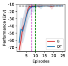
(a) Simple Gridworld

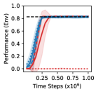
(b) Empty10x10

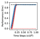
(c) FourRooms

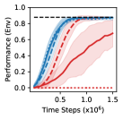
(d) SCS9N1

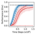
(e) LCS9N1

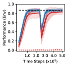
(f) RDS Sequential

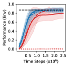
(g) RDS Train (0.35)

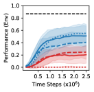
(h) RDS Test (0.25)

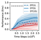
(i) RDS Test (0.35)

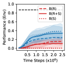
(j) RDS Test (0.45)

Figure 4: The performance of the MIs of DT and B planning in the (a-e) P&L and (f-j) TL settings with (a) tabular and (b-j) NN VE representations. The black dashed lines indicate the performance of the optimal policy in the corresponding environment. The green and magenta dashed line in (a) inidicates the point after which DT and B planning’s models become, and remain as, PXMs, respectively. Shaded regions are one standard error over (a) 100 and (b-j) 50 runs.

P&L Experiments. In Sec. 4.2, we argued that if one were to use tabular VEs and models in the MIs of the two planning styles, the results of the P&L section of Sec. 4.1 would hold exactly. Additionally, we also argued that the performance gap between the two planning styles would reduce in their MIs and even gradually close if the combined models of both planning styles become, and remain as, PXMs. In order to test these, we implemented simplified tabular versions of the MIs of the two planning styles (see Alg. 7 & 8) and compared them on the SG environment. Results are shown in Fig. 4(a). As expected, the results of the P&L section of Sec. 4.1 holds exactly, and the performance gap between the two planning styles indeed reduces and gradually closes after the models become, and remain as, PXMs.

We then argued that although the usage of NNs in the representation of the VEs and models of the two planning styles would not break the performance trend, their implementation details can also play an important role on how they would compare against each other. We hypothesized that although both planning styles would suffer from CMEs, B planning would additionally suffer from updating its VE using potentially harmful simulated experience, and thus it is likely to suffer more in reaching optimal (or close to optimal) performance. To test these hypotheses, we compared the MIs of the two planning styles (see Alg. 5 & 6) on several MG environments. In order to test the effect of CMEs in DT planning, we performed experiments in which the parametric model is unrolled for 1, 5, and 15 time steps during search, denoted as DT(1), DT(5) and DT(15). Note that CMEs are not a problem for B planning, as its parametric model is only unrolled for a single time step. Also, in order to test the effect of updating the VE with simulated experience in B planning, we performed experiments in which its VE is updated with only real, both real and simulated, and only simulated experience, denoted as B(R), B(R+S) and B(S). See App. G.2 for the details of these experiments. The results, in Fig. 4(b)-4(e), show that even though the performance of DT planning degrades slightly with the increase in CMEs, this can indeed be easily mitigated by decreasing the search budget. However, as can be seen, even without any CMEs, just the usage of simulated experience alone can indeed slowdown, or even prevent (as in B(S)), B planning in reaching optimal (or close to optimal) performance, especially in environments that are harder to model such as SCS9N1 & LCS9N1.

TL Experiments. In Sec. 4.2, we first argued that B planning would again suffer more in reaching optimal (or close to optimal) performance on the TRTs in both TL settings. Then, we hypothesized that B planning would also suffer more in adapting to the subsequent TSTs in the first TL setting. Finally, we hypothesized that, under certain assumptions, DT planning would perform better than B planning on the TSTs in the second TL setting. In order to test the first two of these hypotheses, we compared the MIs of the two planning styles on a sequential version of the RDS environment [32] (see App. G.2 for the details). Results in Fig. 4(f) show that, similar to the P&L setting, the increasing usage of simulated experience can indeed slowdown, or even prevent (as in B(S)), B planning in reaching optimal (or close to optimal) performance on the TRTs, and that B planning indeed suffers more in adapting to the TSTs. And, in order to test the first and third hypotheses, we compared the two planning styles on the exact RDS environment. Results are shown in Fig. 4(g)-4(j). As can be seen, the increasing usage of simulated experience can again slowdown, or even prevent (as in B(S)), B planning in reaching optimal (or close to optimal) performance on the TRTs. We can also see that DT planning indeed achieves significantly better performance than B planning across all TSTs with varying difficulties.

6 Related Work

The abstract view that we provide in this study is mostly related to the recent monograph of Bertsekas [7] in which the recent successes of AlphaZero [21], a DT planning algorithm, are viewed through the lens of DP. However, we take a broader perspective and provide a unified view that encompasses both DT and B planning algorithms. Also, instead of assuming the availability of an exact model, we consider the scenario in which a model has to be learned by pure interaction with the environment. Another closely related study is the study of Hamrick et al. [14] which informally relates MuZero [19], another DT planning algorithm, to various other DT and B planning algorithms in the literature. Our study can be viewed as a study that formalizes the relation between the two planning styles. There have also been studies that empirically compare the performances of various DT and B planning algorithms on continuous control domains in the P&L setting [31], and on MG environments in specific TL settings [32]. However, none of these studies provide a general understanding of when will one planning style perform better than the other.

Finally, our work also has connections to the studies of Jiang et al. [16] and Arumugam et al. [3] which provide upper bounds for the performance difference between policies generated as a result of planning with an exact model and an estimated model. However, rather than providing upper bounds, in this study, we are instead interested in understanding which classes of models will allow for one planning style to perform better than the other. Lastly, another related line of research is the recent studies of Grimm et al. [11, 12] which classify models according to how relevant they are for value-based planning. Although, we share the same overall idea that models should only be judged for how useful they are in the planning process, our work differs in that we classify the models according to how useful they are in the comparison of the two planning styles.

7 Conclusion and Discussion

To summarize, we first viewed the CIs and MIs of DT and B planning in a unified way through the lens of DP, and then provided theoretical results and hypotheses on which one will perform better than the other across a variety of settings. Then, we empirically validated these results through illustrative experiments. Overall, our findings suggest that even though DT planning does not perform as well as B planning in their CIs, due to the reasons detailed in this study, the MIs of it can perform on par or better than their B planning counterparts in both the P&L and TL settings. In this study, our main goal was to understand under what conditions and in which settings one planning style will perform better than the other in fast-response-requiring domains, and not to provide any practical insights at the moment. However, we believe that both the proposed unifying framework and our theoretical and empirical results can be helpful to the community in improving the two planning styles in potentially interesting ways. Also note that we were only interested in comparing the two planning styles in terms of the expected discounted return of their output policies. Though not the main focus of this study, other possible interesting comparison directions include comparing in terms of sample efficiency and real-time performance. Lastly, due to their easy-to-learn optimal policies and their suitability in designing controlled experiments, we have mainly performed our MI experiments on MG environments. However, experiments in other environments can be helpful in further validating the hypotheses of this study. We hope to tackle this in future work.

Checklist

1. For all authors…

   1. Do the main claims made in the abstract and introduction accurately reflect the paper’s contributions and scope? [Yes]

   2. Did you describe the limitations of your work? [Yes] In the second paragraph of Sec. 7, we discussed the current limitations of this study, and we have also provided potential future work directions.

   3. Did you discuss any potential negative societal impacts of your work? [N/A] Our paper studies how the two prevalent planning styles in model-based RL, decision-time and background planning, would compare against each other across a variety of settings. We believe that this should not have any negative societal impacts.

   4. Have you read the ethics review guidelines and ensured that your paper conforms to them? [Yes]

2. If you are including theoretical results…

   1. Did you state the full set of assumptions of all theoretical results? [Yes] Our assumptions are in Sec. 2 and 4.

   2. Did you include complete proofs of all theoretical results? [Yes] Our complete proofs are in App. C.

3. If you ran experiments…

   1. Did you include the code, data, and instructions needed to reproduce the main experimental results (either in the supplemental material or as a URL)? [Yes] We have provided both the instructions and code to reproduce our results in App. G.

   2. Did you specify all the training details (e.g., data splits, hyperparameters, how they were chosen)? [Yes] Our implementation details are in App. G.

   3. Did you report error bars (e.g., with respect to the random seed after running experiments multiple times)? [Yes] All of our plots contain error bars.

   4. Did you include the total amount of compute and the type of resources used (e.g., type of GPUs, internal cluster, or cloud provider)? [No]

4. If you are using existing assets (e.g., code, data, models) or curating/releasing new assets…

   1. If your work uses existing assets, did you cite the creators? [Yes] We cite the creator of the code we use in App. E.

   2. Did you mention the license of the assets? [No] The code that we use is already publicly available.

   3. Did you include any new assets either in the supplemental material or as a URL? [No]

   4. Did you discuss whether and how consent was obtained from people whose data you’re using/curating? [N/A]

   5. Did you discuss whether the data you are using/curating contains personally identifiable information or offensive content? [N/A]

5. If you used crowdsourcing or conducted research with human subjects…

   1. Did you include the full text of instructions given to participants and screenshots, if applicable? [N/A]

   2. Did you describe any potential participant risks, with links to Institutional Review Board (IRB) approvals, if applicable? [N/A]

   3. Did you include the estimated hourly wage paid to participants and the total amount spent on participant compensation? [N/A]

Appendix A Pseudocodes of the CIs of the Two Planning Styles

Algorithm 1 Tabular Online Monte-Carlo Planning (OMCP) [28] with an Adaptable Model

1:Initialize $\pi^{i}\in\mathbb{\Pi}$ as a random policy

2:Initialize $\bar{m}(s,a)$ $\forall s\in\mathcal{S}$ & $\forall a\in\mathcal{A}$

3:$n_{r}\leftarrow\text{number of episodes to perform rollouts}$

4:while $\bar{m}$ has not converged do

5:     $S\leftarrow\text{reset environment}$

6:     while not done do

7:         $A\leftarrow\epsilon\text{-greedy}(\text{MC\_rollout}(S,\bar{m},n_{r},\pi^{i}))$

8:         $R,S^{\prime},\text{done}\leftarrow\text{environment($A$)}$

9:         Update $\bar{m}(S,A)$ with $R$, $S^{\prime}$, done

10:         $S\leftarrow S^{\prime}$

11:     end while

12:end while

13:Return $\bar{m}(s,a)$

Algorithm 2 Tabular Exhaustive Search [9] with an Adaptable Model

1:Initialize $\bar{m}(s,a)$ $\forall s\in\mathcal{S}$ & $\forall a\in\mathcal{A}$

2:$h\leftarrow\text{search heuristic}$

3:while $\bar{m}$ has not converged do

4:     $S\leftarrow\text{reset environment}$

5:     while not done do

6:         $A\leftarrow\epsilon\text{-greedy}(\text{exhaustive\_tree\_search}(S,\bar{m},h))$

7:         $R,S^{\prime},\text{done}\leftarrow\text{environment($A$)}$

8:         Update $\bar{m}(S,A)$ with $R$, $S^{\prime}$, done

9:         $S\leftarrow S^{\prime}$

10:     end while

11:end while

12:Return $\bar{m}(s,a)$

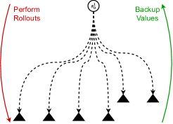
(a) Pure Rollouts

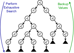
(b) Pure Search

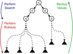
(c) Search + Rollouts

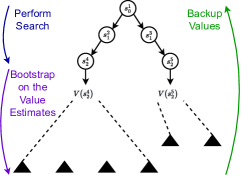
(d) Search + Bootstrapping on the value estimates

Figure A.1: Various planning styles within DT planning in which planning is performed (i) by purely performing rollouts, (ii) by purely performing search, (iii) by performing rollouts after performing some amount of search, and (iv) by bootstrapping on the value estimates after performing some amount of search. The subscripts and the superscripts on the states indicate the time steps and state identifiers, respectively. The black traingles indicate the terminal states.

Algorithm 3 General Tabular Dyna-Q [22, 23]

1:Initialize $Q(s,a)$ $\forall s\in\mathcal{S}$ & $\forall a\in\mathcal{A}$

2:Initialize $\bar{\bar{m}}(s,a)$ $\forall s\in\mathcal{S}$ & $\forall a\in\mathcal{A}$

3:$\mathcal{SA}_{\text{prev}}\leftarrow\{\}$

4:$n_{p}\leftarrow\text{number of time steps to perform planning}$

5:while $Q$ and $\bar{\bar{m}}$ has not converged do

6:     $S\leftarrow\text{reset environment}$

7:     while not done do

8:         $A\leftarrow\epsilon\text{-greedy}(Q(S,\cdot))$

9:         $R,S^{\prime},\text{done}\leftarrow\text{environment($A$)}$

10:         $\mathcal{SA}_{\text{prev}}\leftarrow\mathcal{SA}_{\text{prev}}+\{(S,A)\}$

11:         Update $Q(S,A)$ with $R$, $S^{\prime}$, done

12:         Update $\bar{\bar{m}}(S,A)$ with $R$, $S^{\prime}$, done

13:         $i\leftarrow 0$

14:         while $i<n_{p}$ do

15:              $S_{\bar{\bar{m}}},A_{\bar{\bar{m}}}\leftarrow\text{sample from }\mathcal{SA}_{\text{prev}}$

16:              $R_{\bar{\bar{m}}},S_{\bar{\bar{m}}}^{\prime},\text{done}_{\bar{\bar{m}}}\leftarrow\bar{\bar{m}}(S_{\bar{\bar{m}}},A_{\bar{\bar{m}}})$

17:              Update $Q(S_{\bar{\bar{m}}},A_{\bar{\bar{m}}})$ with $R_{\bar{\bar{m}}}$, $S_{\bar{\bar{m}}}^{\prime}$, $\text{done}_{\bar{\bar{m}}}$

18:              $i\leftarrow i+1$

19:         end while

20:         $S\leftarrow S^{\prime}$

21:     end while

22:end while

23:Return $Q(s,a)$

Algorithm 4 Tabular Dyna-Q of Interest

1:Initialize $Q(s,a)$ $\forall s\in\mathcal{S}$ & $\forall a\in\mathcal{A}$

2:Initialize $\bar{\bar{m}}(s,a)$ $\forall s\in\mathcal{S}$ & $\forall a\in\mathcal{A}$

3:while $Q$ and $\bar{\bar{m}}$ has not converged do

4:     $S\leftarrow\text{reset environment}$

5:     while not done do

6:         $A\leftarrow\epsilon\text{-greedy}(Q(S,\cdot))$

7:         $R,S^{\prime},\text{done}\leftarrow\text{environment($A$)}$

8:         Update $\bar{\bar{m}}(S,A)$ with $R$, $S^{\prime}$, done

9:         $S\leftarrow S^{\prime}$

10:     end while

11:     while $Q$ has not converged do

12:         $S_{\bar{\bar{m}}},A_{\bar{\bar{m}}}\leftarrow\text{sample from }\mathcal{S}\times\mathcal{A}$

13:         $R_{\bar{\bar{m}}},S_{\bar{\bar{m}}}^{\prime},\text{done}_{\bar{\bar{m}}}\leftarrow\bar{\bar{m}}(S_{\bar{\bar{m}}},A_{\bar{\bar{m}}})$

14:         Update $Q(S_{\bar{\bar{m}}},A_{\bar{\bar{m}}})$ with $R_{\bar{\bar{m}}}$, $S_{\bar{\bar{m}}}^{\prime}$, $\text{done}_{\bar{\bar{m}}}$

15:     end while

16:end while

17:Return $Q(s,a)$

Appendix B Discussion on the Choice of the CIs of the Two Planning Styles

As indicated in the main paper, for DT planning, we study the OMCP algorithm of Tesauro and Galperin [28], and, for B planning, we study the Dyna-Q algorithm of Sutton [22, 23]. We choose these algorithms as they are easy to analyze. In this study, as we are interested in scenarios where the model has to be learned from pure interaction, we consider a version of the OCMP algorithm in which a parametric model is learned from experience (see Alg. 1 for the pseudocode). Note that this is the only difference compared to the original version of the OMCP algorithm. And, in order to make a fair comparison with this version of the OMCP algorithm, we consider a simplified version of the Dyna-Q algorithm (see Alg. 3 & 4 for the pseudocodes of the original and simplified versions, respectively). Compared to the original version of Dyna-Q, in this version, there are several minor differences:

• While planning, the agent can now sample states and actions that it has not observed or taken before. Note that this is also the case for the version of the OMCP algorithm considered in this study.

• Now, instead of using samples from both the environment and model, the agent updates its VE with samples only from the model. Note that the version of the OMCP algorithm considered in this study also makes use of only the model while performing planning.

• Now, instead of planning for a fixed number of time steps, the agent performs planning until its VE converges. Note that, in order to allow for sample efficiency, usually $n_{p}$ is also set to high values in the original version of the Dyna-Q algorithm. Also note that, in order to properly evaluate the base policy, usually $n_{r}$ is also set to high values in the version of the OMCP algorithm considered in this study. Thus, in practice, both the original version of the Dyna-Q algorithm and the version of the OMCP algorithm considered in this study also devote a significant budget to perform planning.

• Lastly, instead of performing planning after every time step, now the agent only performs planning after every episode. Rather than to allow for a fair comparison, this is to allow the Dyna-Q version of interest to be able operate in fast-response-requiring domains (planning until convergence after every time step would obviously slow down the response time of the algorithm and prevent it from operating in fast-response-requiring domains).

Appendix C Proofs

Proposition 1.

Let $m\in\mathcal{M}$ be a PCM of $m^{*}$ w.r.t. $\Pi=\{\pi_{m}^{r},\pi_{m}^{ce}\}\subseteq\mathbb{\Pi}$ and $J$. Then, $J_{m^{*}}^{\pi_{m}^{r}}\geq J_{m^{*}}^{\pi_{m}^{ce}}$.

Proof.

This result directly follows from Defn. 1 & 5. Recall that, according to Defn. 5, given a $\pi^{b}\in\mathbb{\Pi}$, $\pi_{m}^{r}$ and $\pi_{m}^{ce}$ are the policies that are obtained after performing one-step PI and full VI on top of a $\pi^{b}$ in model $m$, respectively. Thus, we have $J_{m}^{\pi_{m}^{r}}\leq J_{m}^{\pi_{m}^{ce}}$ [8], which, by Defn. 1, implies $J_{m^{*}}^{\pi_{m}^{r}}\geq J_{m^{*}}^{\pi_{m}^{ce}}$. ∎

Proposition 2.

Let $m\in\mathcal{M}$ be a PRM of $m^{*}$ w.r.t. $\Pi=\{\pi_{m}^{r},\pi_{m}^{ce}\}\subseteq\mathbb{\Pi}$ and $J$. Then, $J_{m^{*}}^{\pi_{m}^{ce}}\geq J_{m^{*}}^{\pi_{m}^{r}}$.

Proof.

This result directly follows from Defn. 2 & 5. Recall that, according to Defn. 5, given a $\pi^{b}\in\mathbb{\Pi}$, $\pi_{m}^{r}$ and $\pi_{m}^{ce}$ are the policies that are obtained after performing one-step PI and full VI on top of a $\pi^{b}$ in model $m$, respectively. Thus, we have $J_{m}^{\pi_{m}^{r}}\leq J_{m}^{\pi_{m}^{ce}}$ [8], which, by Defn. 2, implies $J_{m^{*}}^{\pi_{m}^{ce}}\geq J_{m^{*}}^{\pi_{m}^{r}}$. ∎

Proposition 3.

Let $\bar{m}\in\mathcal{M}$ be a PCM or a PRM of $m^{*}$ w.r.t. $\bar{\Pi}=\{\pi_{\bar{m}}^{r},\pi_{\bar{m}}^{ce}\}\subseteq\mathbb{\Pi}$ and $J$, and let $\bar{\bar{m}}\in\mathcal{M}$ be a PNM of $m^{*}$ w.r.t. $\bar{\bar{\Pi}}=\{\pi_{\bar{\bar{m}}}^{r},\pi_{\bar{\bar{m}}}^{ce}\}\subseteq\mathbb{\Pi}$ and $J$. Then, $J_{m^{*}}^{\pi_{\bar{m}}^{r}}\geq J_{m^{*}}^{\pi_{\bar{\bar{m}}}^{ce}}$.

Proof.

This result directly follows from Defn. 3 & 5. Recall that, according to Defn. 5, given a $\pi^{b}\in\mathbb{\Pi}$, $\pi_{\bar{\bar{m}}}^{ce}$ is the policy that is obtained after performing full VI on top of $\pi^{b}$ in model $\bar{\bar{m}}$. Thus, $\pi_{\bar{\bar{m}}}^{ce}$ is one of the optimal policies of model $\bar{\bar{m}}$ [8], which, by Defn. 3, implies $J_{m^{*}}^{\pi_{\bar{\bar{m}}}^{ce}}=\min_{\pi\in\Pi}J_{m^{*}}^{\pi}$ and thus $J_{m^{*}}^{\pi_{\bar{\bar{m}}}^{ce}}\leq J_{m^{*}}^{\pi}\forall\pi\in\mathbb{\Pi}$. This in turn implies $J_{m^{*}}^{\pi_{\bar{m}}^{r}}\geq J_{m^{*}}^{\pi_{\bar{\bar{m}}}^{ce}}$. ∎

Proposition 4.

Let $\bar{m}\in\mathcal{M}$ be a PCM or a PRM of $m^{*}$ w.r.t. $\bar{\Pi}=\{\pi_{\bar{m}}^{r},\pi_{\bar{m}}^{ce}\}\subseteq\mathbb{\Pi}$ and $J$, and let $\bar{\bar{m}}\in\mathcal{M}$ be a PXM of $m^{*}$ w.r.t. $\bar{\bar{\Pi}}=\{\pi_{\bar{\bar{m}}}^{r},\pi_{\bar{\bar{m}}}^{ce}\}\subseteq\mathbb{\Pi}$ and $J$. Then, $J_{m^{*}}^{\pi_{\bar{\bar{m}}}^{ce}}\geq J_{m^{*}}^{\pi_{\bar{m}}^{r}}$.

Proof.

This result directly follows from Defn. 4 & 5. Recall that, according to Defn. 5, given a $\pi^{b}\in\mathbb{\Pi}$, $\pi_{\bar{\bar{m}}}^{ce}$ is the policy that is obtained after performing full VI on top of $\pi^{b}$ in model $\bar{\bar{m}}$. Thus, $\pi_{\bar{\bar{m}}}^{ce}$ is one of the optimal policies of model $\bar{\bar{m}}$ [8], which, by Defn. 4, implies $J_{m^{*}}^{\pi_{\bar{\bar{m}}}^{ce}}=\max_{\pi\in\Pi}J_{m^{*}}^{\pi}$ and thus $J_{m^{*}}^{\pi_{\bar{\bar{m}}}^{ce}}\geq J_{m^{*}}^{\pi}\forall\pi\in\mathbb{\Pi}$. This in turn implies $J_{m^{*}}^{\pi_{\bar{\bar{m}}}^{ce}}\geq J_{m^{*}}^{\pi_{\bar{m}}^{r}}$. ∎

Appendix D Pseudocodes of the MIs of the Two Planning Styles

Algorithm 5 The DT Planning Algorithm in Zhao et al. [32]

1:Initialize the parameters $\theta$, $\eta$ & $\omega$ of $\phi_{\theta}:\mathcal{O}_{E}\to\mathcal{S}_{A}$, $Q_{\eta}:\mathcal{S}_{A}\times\mathcal{A}_{E}\to\amsmathbb{R}$ & $\bar{m}_{p\omega}=(p_{\omega},r_{\omega},d_{\omega})$

2:Initialize the replay buffer $\bar{m}_{np}\leftarrow\{\}$

3:$N_{ple}\leftarrow\text{number of episodes to perform planning and learning}$

4:$N_{rbt}\leftarrow\text{number of samples that the replay buffer must hold to perform planning and learning}$

5:$n_{s}\leftarrow\text{number of time steps to perform search}$

6:$n_{bs}\leftarrow\text{number of samples to sample from }\bar{m}_{np}$

7:$h\leftarrow\text{search heuristic}$

8:$S\leftarrow\text{replay buffer sampling strategy}$

9:$i\leftarrow 0$

10:while $i<N_{ple}$ do

11:     $O\leftarrow\text{reset environment}$

12:     while not done do

13:         $A\leftarrow\epsilon\text{-greedy}(\text{tree\_search\_with\_bootstrapping}(\phi_{\theta}(O),\bar{m}_{p\omega},Q_{\eta},n_{s},h))$

14:         $R,O^{\prime},\text{done}\leftarrow\text{environment($A$)}$

15:         $\bar{m}_{np}\leftarrow\bar{m}_{np}+\{(O,A,R,O^{\prime},\text{done})\}$

16:         if $|\bar{m}_{np}|\geq N_{rbt}$ then

17:              $\mathcal{B}_{np}\leftarrow\text{sample\_batch}(\bar{m}_{np},n_{bs},S)$

18:              Update $\phi_{\theta}$, $Q_{\eta}$ & $\bar{m}_{p\omega}$ with $\mathcal{B}_{np}$

19:         end if

20:         $O\leftarrow O^{\prime}$

21:     end while

22:     $i\leftarrow i+1$

23:end while

24:Return $\phi_{\theta}$, $Q_{\eta}$ & $\bar{m}_{p\omega}$

Algorithm 6 The B Planning Algorithm in Zhao et al. [32]

1:Initialize the parameters $\theta$, $\eta$ & $\omega$ of $\phi_{\theta}:\mathcal{O}_{E}\to\mathcal{S}_{A}$, $Q_{\eta}:\mathcal{S}_{A}\times\mathcal{A}_{E}\to\amsmathbb{R}$ & $\bar{\bar{m}}_{p\omega}=(p_{\omega},r_{\omega},d_{\omega})$

2:Initialize the replay buffer $\bar{\bar{m}}_{np}\leftarrow\{\}$ and the imagined replay buffer $\bar{\bar{m}}_{inp}\leftarrow\{\}$

3:$N_{ple}\leftarrow\text{number of episodes to perform planning and learning}$

4:$N_{rbt}\leftarrow\text{number of samples that the replay buffer must hold to perform planning and learning}$

5:$n_{ibs}\leftarrow\text{number of samples to sample from }\bar{\bar{m}}_{inp}$

6:$n_{bs}\leftarrow\text{number of samples to sample from }\bar{\bar{m}}_{np}$

7:$S\leftarrow\text{replay buffer sampling strategy}$

8:$i\leftarrow 0$

9:while $i<N_{ple}$ do

10:     $O\leftarrow\text{reset environment}$

11:     while not done do

12:         $A\leftarrow\epsilon\text{-greedy}(Q_{\eta}(\phi_{\theta}(O),\cdot))$

13:         $R,O^{\prime},\text{done}\leftarrow\text{environment($A$)}$

14:         $\bar{\bar{m}}_{np}\leftarrow\bar{\bar{m}}_{np}+\{(O,A,R,O^{\prime},\text{done})\}$

15:         $\bar{\bar{m}}_{inp}\leftarrow\bar{\bar{m}}_{inp}+\{(\phi_{\theta}(O),A)\}$

16:         if $|\bar{\bar{m}}_{np}|\geq N_{rbt}$ then

17:              $\mathcal{B}_{inp}\leftarrow\text{sample\_batch}(\bar{\bar{m}}_{inp},n_{ibs},S)$

18:              $\mathcal{B}_{p}\leftarrow\mathcal{B}_{inp}+\bar{\bar{m}}_{p\omega}(\mathcal{B}_{inp})$

19:              $\mathcal{B}_{np}\leftarrow\text{sample\_batch}(\bar{\bar{m}}_{np},n_{bs},S)$

20:              Update $\phi_{\theta}$ & $Q_{\eta}$ with $\mathcal{B}_{np}+\mathcal{B}_{p}$

21:              Update $\phi_{\theta}$ & $\bar{\bar{m}}_{p\omega}$ with $\mathcal{B}_{np}$

22:         end if

23:         $O\leftarrow O^{\prime}$

24:     end while

25:     $i\leftarrow i+1$

26:end while

27:Return $\phi_{\theta}$ & $Q_{\eta}$

Appendix E Discussion on the Choice of the MIs of the Two Planning Styles

As indicated in the main paper, we study the DT and B planning algorithms in Zhao et al. [32]. More specifically, for DT planning, we study the “UP” algorithm, and, for B planning, we study the “Dyna” algorithm in [32]. We choose these algorithms as they are reflective of many of the properties of their state-of-the-art (SOTA) counterparts (MuZero [19] and SimPLe [33] / DreamerV2 [13], respectively) and their code is publicly available. The pseudocodes of these algorithms are presented in Alg. 5 & 6, respectively. Note that, similar to their SOTA counterparts, these two algorithms do not employ the “bottleneck mechanism” introduced in [32]. Some of the important similarities and differences between these algorithms and their SOTA counterparts, are as follows:

1. Similarities and differences between the DT planning algorithm in Zhao et al. [32] and MuZero [19]

   • Similar to MuZero, the DT planning algorithm in [32] also performs planning with both a parametric and non-parametric model.

   • Similar to MuZero, the DT planning algorithm in [32] also represents its parametric model using NNs.

   • Similar to MuZero, the DT planning algorithm in [32] also learns a parametric model through pure interaction with the environment. However, rather than unrolling the model for several time steps and training it with the sum of the policy, value and reward losses as in MuZero, it unrolls the model for only a single time step and trains it with the sum of the value, dynamics, reward and termination losses (see the total loss term in Sec. 3 of [32]).

   • Lastly, similar to MuZero, the DT planning algorithm in [32] selects actions by directly bootstrapping on the value estimates of a continually improving policy (without performing any rollouts), which is obtained by planning with a non-parametric model, after performing some amount search with a parametric model. However, rather than performing the search using Monte-Carlo Tree Search (MCTS, [17]) as in MuZero, it uses best-first search (during training) and random search (during evaluation) (see App. H of [32] for the details of the search procedures).

2. Similarities and differences between the B planning algorithm in Zhao et al. [32] and SimPLe [33] / DreamerV2 [13]

   • Similar to SimPLe / DreamerV2, the B planning algorithm in [32] also performs planning with a parametric model. Additionally, it also performs planning with a non-parametric model.

   • Similar to SimPLe / DreamerV2, the B planning algorithm in [32] also represents its parametric model using NNs and it also updates its VE using the simulated data generated with this model.

   • Similar to SimPLe / DreamerV2, the B planning algorithm in [32] also learns a parametric model through pure interaction with the environment. However, rather than performing planning with this model after allowing for an initial kickstarting period as in SimPLe / DreamerV2 (referred to as a “world model” learning period), for a fair comparison with the DT planning algorithm, it starts to perform planning right at the beginning of the model learning process.

   • Lastly, similar to SimPLe / DreamerV2, the B planning algorithm in [32] selects actions by simply querying its VE.

Even though there are some differences between the planning algorithms in [32] and their SOTA counterparts, except for the kickstarting period in SOTA B planning algorithms, these are just minor implementation details that would not have any impact on the conclusions of this study. Although the kickstarting period can mitigate the harmful simulated data problem to some degree (or even prevent it if the period is sufficiently long), allowing for it would definitely prevent a fair comparison with the DT planning algorithm in [32]. This is why we did not allow for it in our experiments.

Appendix F Discussion on the Combined View of Models

In order to be able to view the DT and B planning algorithms that perform planning with both a parametric and non-parametric model through our proposed DP framework, we view the two separate models of these algorithms as a single combined model. This becomes obvious for B planning algorithms if one notes that they perform planning with a batch of data that is jointly generated by both a parametric and non-parametric model (see e.g., line 20 in Alg. 6 in which $\phi_{\theta}$ and $Q_{\eta}$ are updated with batch of data that is jointly generated by both $\bar{\bar{m}}_{p\omega}$ and $\bar{\bar{m}}_{np}$), which can be thought of performing planning with a batch of data that is generated by a single combined model. It also becomes obvious for DT planning algorithms if one notes that they perform planning by first performing search with a parametric model, and then by bootstrapping on the value estimates of a continually improving policy that is obtained by planning with a non-parametric model (see e.g., line 13 in Alg. 5 in which action selection is done with both $\bar{m}_{p\omega}$ and $Q_{\eta}$ (which is obtained by planning with $\bar{m}_{np}$)), which can be thought of performing planning with a single combined model that is obtained by concatenating the parametric and non-parametric models.

Appendix G Experimental Details

In this section, we provide the details of the experiments that are performed in Sec. 5. This also includes the implementation details of the CIs and MIs of the two planning styles considered in this study.

G.1 Details of the CI Experiments

In all of the CI experiments, we have calculated the performance with a discount factor ($\gamma$) of $0.9$.

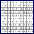
(a) SG Rewards

(b) $m_{8}$ Rewards

(c) Initial PDM Rewards

(d) TST Rewards

Figure G.1: Reward functions of (a) the SG environment, (b) the $m_{8}$ model, (c) the initial PDM, and (d) the TST.

Figure G.2: The form of SA used in this study.

Environment & Models. All of the experiments in Sec. 5.1 are performed on the SG environment. Here, the agent spawns in state S and has to navigate to the goal state depicted by G. At each time step, the agent receives an $(x,y)$ pair, indicating its position, and based on this, selects an action that moves it to one of the four neighboring cells with a slip probability of $0.1$. The agent receives a negative reward that is linearly proportional to its distance from G and a reward of $+10$ if it reaches G (see Fig. 1(a)). The agent-environment interaction lasts for a maximum of 100 time steps, after which the episode terminates with a reward of $0$ if the agent was not able to reach the goal state G. (PP Setting) For the experiments in the PP setting, the agent is provided with series of models in which it receives a reward of $+10$ if it reaches the goal state and a reward of $0$ elsewhere. For example, see the reward function of model $m_{8}$ in Fig. 1(b). Note that these models have the same transition distribution and initial state distribution with the SG environment. (P&L Setting) For the experiments in the P&L setting, the models of both of the planning styles are initialized as a hand-designed PDM with a reward function as in Fig. 1(c) and with a goal state located at the bottom right corner. Note that in these experiments, we have assumed that the agent already has access to the transition distribution and initial state distribution of the environment, and only has to learn the reward function. (TL Setting) Finally, for the experiments in the TL setting, we considered a TST with a reward function as in Fig. 1(d), which is a transposed version of the TRT’s reward function (see Fig. 1(a)). Note again that we have assumed that the agent already has access to the transition distribution and initial state distribution of the environment, and only has to learn the reward function.

Implementation Details of the CIs. For our CI experiments, we considered specific versions of the OMCP algorithm of Tesauro and Galperin [28] and the Dyna-Q algorithm of Sutton [22, 23]. The pseudocodes of these algorithms are presented in Alg. 1 & 4, respectively, and the details of them are provided in Table G.1 & G.2, respectively. Note that in Alg. 1, $n_{r}$ (the number of episodes to perform rollouts) is set to a high value so that the input policy $\pi^{i}$ can properly be evaluated.

Table G.1: Details and hyperparameters of Alg. 1.

$\pi^{i}$	a deterministic random policy
$\bar{m}$	a tabular model (initialized as a hand-designed PDM (see Fig. 1(c)))
$n_{r}$	50
$\epsilon$	linearly decays from $1.0$ to $0.0$ over the first 20 episodes
SA (in FA experiments)	an aggregation of the form in Fig. G.2

Table G.2: Details and hyperparameters of Alg. 4.

$Q$	a tabular value function (initialized as zero $\forall s\in\mathcal{S}$ and $\forall a\in\mathcal{A}$)
$\bar{\bar{m}}$	a tabular model (initialized as a hand-designed PDM (see Fig. 1(c)))
$\epsilon$	linearly decays from $1.0$ to $0.0$ over the first 20 episodes
SA (in FA experiments)	an aggregation of the form in Fig. G.2

G.2 Details of the MI Experiments

In all of the MI experiments on the SG environment, we have calculated the performance with a discount factor ($\gamma$) of $0.9$, and in all of the MI experiments on the MG environments, we have calculated the performance with a discount factor of $0.99$.

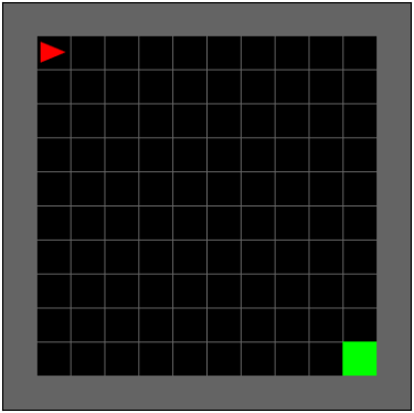
(a) Empty 10x10

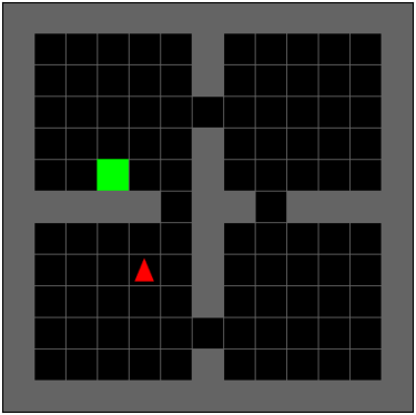
(b) FourRooms

(c) SCS9N1

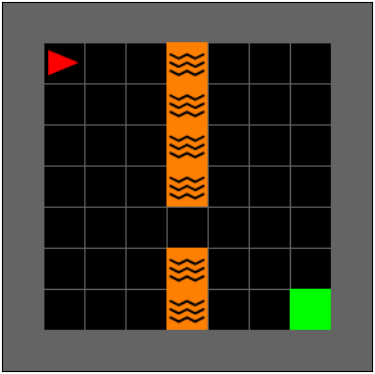
(d) LCS9N1

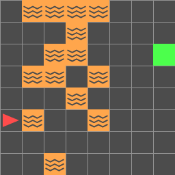
(e) RDS Train (0.35)

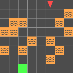
(f) RDS Test (0.25)

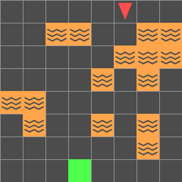
(g) RDS Test (0.35)

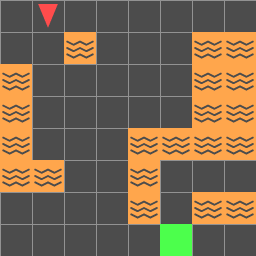
(h) RDS Test (0.45)

Figure G.3: (a-d) Several environments that either pre-exist in or are manually built on top of MG. (e-h) The TRTs and TSTs of varying difficulty in the RDS environment [32]. Note that the TSTs are just transposed versions of the TRTs.

Environments & Models. In Sec. 5.2, part of our experiments were performed both on the SG environment and part of them were performed on MG environments. The details of these environments and their corresponding models are as follows:

• SG Environment. To learn about the SG environment, we refer the reader to Sec. G.1 as we have used the same environment in the MI experiments as well. (P&L Setting) To learn about the models of both planning styles, we also refer the reader to the P&L Setting of Sec. G.1 as have used the same models in the MI experiments as well.

• MG Environments. In the MG environments, the agent, depicted in red, has to navigate to the green goal cell while avoiding the orange lava cells (if there are any). At each time step, the agent receives a grid-based observation that contains its own position and the positions of the goal, wall and lava cells, and based on this, selects an action that either turns it left or right, or steps it forward. If the agent steps on a lava cell, the episode terminates with no reward, and if it reaches the goal cell, the episode terminates with a reward of $+1$. More on the details of these environments can be found in Chevalier-Boisvert et al. [10]. (P&L Setting) For the P&L setting, we performed experiments on the Empty 10x10, FourRooms, SimpleCrossingS9N1 (SCS9N1) and LavaCrossingS9N1 (LCS9N1) environments (see Fig. 3(a), 3(b), 3(c), & 3(d), respectively). While the last two of these environments already pre-exist in MG, the first two of them are manually built environments. Specifically, the Empty 10x10 environment is obtained by expanding the Empty 8x8 environment and the 10x10 FourRooms environment is obtained by contracting the 16x16 FourRooms environment in Chevalier-Boisvert et al. [10]. (TL Setting) For the TL setting, we performed experiments on the sequential and regular versions of the RDS environment considered in [32] (see Fig. 3(e)-3(h)). In the sequential version, which we call RDS Sequential, the agent is trained on TRTs with difficulty 0.35 (see Fig. 3(e)) and then it is allowed to adapt to subsequent TSTs (a transposed version of the TRTs) with difficulty 0.35 (see Fig. 3(g)). In the regular version (the version considered in [32]), the agent is trained on TRTs with difficulty 0.35 (see Fig. 3(e)) and during the training process it is periodically evaluated on TSTs with difficulties varying from 0.25 to 0.45 (see Fig. 3(f)-3(h)). Note that the difficulty parameter here controls the density of the lava cells. Also note that with every reset of the episode, a new lava cell pattern is (procedurally) generated for both the TRTs and TSTs. More on the details of the RDS environment can be found in [32].

  Finally, note that, as opposed to the experiments on SG environment, for both the P&L and TL settings, we did not enforce any kind of structure on the models of the agent, and just initialized them randomly. We also note that, in our experiments with RDS Sequential, we reinitialized the non-parametric models (replay buffers) of both planning styles after the tasks switch from the TRTs to the TSTs.

Implementation Details of the MIs. For our MI experiments, we considered the DT and B planning algorithms in Zhao et al. [32] (see Sec. E), whose pseudocodes are presented in Alg. 5 & 6, respectively. The details of these algorithms are provided in Table G.3 & G.4, respectively. For more details (such as the NN architectures, replay buffer sizes, learning rates, exact details of the tree search, …), we refer the reader to the publicly available code and the supplementary material of [32].

Table G.3: Details and hyperparameters of Alg. 5.

$\phi_{\theta}$	MiniGrid bag of words feature extractor
$Q_{\eta}$	regular NN (P&L setting), NN with attention (for set-based representations) (TL setting)
$\bar{m}_{p\omega}$	regular NN (P&L setting), NN with attention (for set-based representations) (TL setting)
	(bottleneck mechanism is disabled for both of the setting)
$N_{ple}$	$50$M
$N_{rbt}$	$50$k
$n_{s}$	$1$ (DT(1)), $5$ (DT(5)), $15$ (DT(15))
$n_{bs}$	$128$ (P&L setting), $64$ (TL setting)
$h$	best-first search (training), random search (evaluation)
$S$	random sampling
$\epsilon$	linearly decays from $1.0$ to $0.0$ over the first 1M time steps

Table G.4: Details and hyperparameters of Alg. 6.

$\phi_{\theta}$	MiniGrid bag of words feature extractor
$Q_{\eta}$	regular NN (P&L setting), NN with attention (for set-based representations)
	(TL setting)
$\bar{\bar{m}}_{p\omega}$	regular NN (P&L setting), NN with attention (for set-based representations)
	(TL setting) (bottleneck mechanism is disabled for both of the settings)
$N_{ple}$	$50$M
$N_{rbt}$	$50$k
$(n_{ibs},n_{bs})$	$(0,128)$ (B(R)), $(128,128)$ (B(R+S)), $(128,0)$ (B(S)) (P&L setting),
	$(0,64)$ (B(R)), $(64,64)$ (B(R+S)), $(64,0)$ (B(S)) (TL setting)
$S$	random sampling
$\epsilon$	linearly decays from $1.0$ to $0.0$ over the first 1M time steps

Note that the publicly available code of [32] only contains B planning algorithms in which the model is a model over the observations (and not the states), which for some reason causes the B planning algorithm of interest to perform very poorly (see the plots in [32]). For this reason and in order to make a fair comparison with DT planning, we have implemented a version of the B planning algorithm in which the model is a model over the states and we performed all of our experiments with this version of the algorithm. Also note that, while we have used regular representations in our P&L experiments, in order to deal with the large number of tasks, we have made use of set-based representations in our TL experiments (see [32] for the details of this representation).

Additionally, we also performed experiments with simplified tabular versions of the MIs of the two planning styles, whose pseudocodes are presented in Alg. 7 & 8, respectively. The details of these algorithms are provided in Table G.5 & G.6, respectively.

Algorithm 7 Modernized Version of Tabular OMCP with both a Parametric and Non-Parametric Model

1:Initialize $Q(s,a)$ $\forall s\in\mathcal{S}$ & $\forall a\in\mathcal{A}$

2:Initialize $\bar{m}_{p}(s,a)$ $\forall s\in\mathcal{S}$ & $\forall a\in\mathcal{A}$

3:Initialize the replay buffer $\bar{m}_{np}\leftarrow\{\}$

4:$n_{s}\leftarrow\text{number of time steps to perform search}$

5:$h\leftarrow\text{search heuristic}$

6:while $\bar{m}_{p}$ and $\bar{m}_{np}$ has not converged do

7:     $S\leftarrow\text{reset environment}$

8:     while not done do

9:         $A\leftarrow\epsilon\text{-greedy}(\text{tree\_search\_with\_bootstrapping}(S,\bar{m}_{p},Q,n_{s},h))$

10:         $R,S^{\prime},\text{done}\leftarrow\text{environment($A$)}$

11:         $\bar{m}_{np}\leftarrow\bar{m}_{np}+\{(S,A,R,S^{\prime},\text{done})\}$

12:         $S_{\bar{m}_{np}},A_{\bar{m}_{np}},R_{\bar{m}_{np}},S_{\bar{m}_{np}}^{\prime},\text{done}_{\bar{m}_{np}}\leftarrow\text{sample from }\bar{m}_{np}$

13:         Update $Q$ & $\bar{m}_{p}$ with $S_{\bar{m}_{np}},A_{\bar{m}_{np}},R_{\bar{m}_{np}},S_{\bar{m}_{np}}^{\prime},\text{done}_{\bar{m}_{np}}$

14:         $S\leftarrow S^{\prime}$

15:     end while

16:end while

17:Return $Q$ & $\bar{m}_{p}(s,a)$

Algorithm 8 Modernized Version of Tabular Dyna-Q of Interest with both a Parametric and Non-Parametric Model

1:Initialize $Q(s,a)$ $\forall s\in\mathcal{S}$ & $\forall a\in\mathcal{A}$

2:Initialize $\bar{\bar{m}}_{p}(s,a)$ $\forall s\in\mathcal{S}$ & $\forall a\in\mathcal{A}$

3:Initialize the replay buffer $\bar{\bar{m}}_{np}\leftarrow\{\}$

4:while $Q$, $\bar{\bar{m}}_{p}$ and $\bar{\bar{m}}_{np}$ has not converged do

5:     $S\leftarrow\text{reset environment}$

6:     while not done do

7:         $A\leftarrow\epsilon\text{-greedy}(Q(S,\cdot))$

8:         $R,S^{\prime},\text{done}\leftarrow\text{environment($A$)}$

9:         Update $\bar{\bar{m}}_{p}(S,A)$ with $R$, $S^{\prime}$, done

10:         $\bar{\bar{m}}_{np}\leftarrow\bar{\bar{m}}_{np}+\{(S,A,R,S^{\prime},\text{done})\}$

11:         $S\leftarrow S^{\prime}$

12:     end while

13:     while $Q$ has not converged do

14:         $S_{\bar{\bar{m}}_{p}},A_{\bar{\bar{m}}_{p}}\leftarrow\text{sample from }\mathcal{S}\times\mathcal{A}$

15:         $R_{\bar{\bar{m}}_{p}},S_{\bar{\bar{m}}_{p}}^{\prime},\text{done}_{\bar{\bar{m}}_{p}}\leftarrow\bar{\bar{m}}_{p}(S_{\bar{\bar{m}}_{p}},A_{\bar{\bar{m}}_{p}})$

16:         Update $Q(S_{\bar{\bar{m}}_{p}},A_{\bar{\bar{m}}_{p}})$ with $R_{\bar{\bar{m}}_{p}}$, $S_{\bar{\bar{m}}_{p}}^{\prime}$, $\text{done}_{\bar{\bar{m}}_{p}}$

17:         $S_{\bar{\bar{m}}_{np}},A_{\bar{\bar{m}}_{np}},R_{\bar{\bar{m}}_{np}},S_{\bar{\bar{m}}_{np}}^{\prime},\text{done}_{\bar{\bar{m}}_{np}}\leftarrow\text{sample from }\bar{\bar{m}}_{np}$

18:         Update $Q(S_{\bar{\bar{m}}_{np}},A_{\bar{\bar{m}}_{np}})$ with $R_{\bar{\bar{m}}_{np}}$, $S_{\bar{\bar{m}}_{np}}^{\prime}$, $\text{done}_{\bar{\bar{m}}_{np}}$

19:     end while

20:end while

21:Return $Q(s,a)$

Table G.5: Details and hyperparameters of Alg. 7.

$Q$	a tabular value function (initialized as zero $\forall s\in\mathcal{S}$ and $\forall a\in\mathcal{A}$)
$\bar{m}_{p}$	a tabular model (initialized as a hand-designed PDM (see Fig. 1(c)))
$n_{s}$	$|\mathcal{A}|$
$h$	breadth-first search
$\epsilon$	linearly decays from $1.0$ to $0.0$ over the first 20 episodes

Table G.6: Details and hyperparameters of Alg. 8.

$Q$	a tabular value function (initialized as zero $\forall s\in\mathcal{S}$ and $\forall a\in\mathcal{A}$)
$\bar{\bar{m}}_{p}$	a tabular parametric model (initialized as a hand-designed PDM (see Fig. 1(c)))
$\epsilon$	linearly decays from $1.0$ to $0.0$ over the first 20 episodes

Appendix H Additional Results

In this section, we provide complementary results to our empirical results in Sec. 5. Specifically, we provide (i) performance plots that are obtained by evaluating the different planning styles in their corresponding models and (ii) total reward plots that are obtained by evaluating the different planning styles in both the considered environments and in their corresponding models. Note that while the performance plots are obtained by the measure in (1), the total reward plots are obtained by simply adding the rewards obtained by the agent throughout the episodes (which is actually the expected undiscounted return, i.e., when we use $\gamma=1.0$ in measure (1)).

H.1 Experiments with CIs

H.1.1 PP Experiments

(a) Tabular

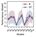
(b) State Aggregarion

Figure H.1: The performance of the CIs of DT and B planning in their corresponding models (learned on the SG environment) in the PP setting with tabular and SA VE representations. Shaded regions are one standard error over 100 runs.

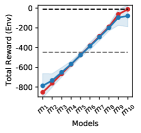
(a) Tabular

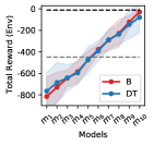
(b) State Aggregation

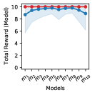
(c) Tabular

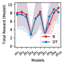
(d) State Aggregation

Figure H.2: The total reward obtained by the CIs of DT and B planning (a, b) on the SG environment and (c, d) in their corresponding models (learned on the SG environment) in the PP setting with tabular and SA VE representations. Black & gray dashed lines indicate total reward obtained by the optimal & random policies, respectively. Shaded regions are one standard error over 100 runs.

H.1.2 P&L Experiments

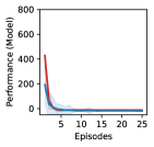
(a) Tabular

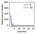
(b) State Aggregation

Figure H.3: The performance of the CIs of DT and B planning in their corresponding models (learned on the SG environment) in the P&L setting with tabular and SA VE representations. Shaded regions are one standard error over 100 runs.

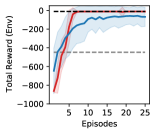
(a) Tabular

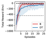
(b) State Aggregation

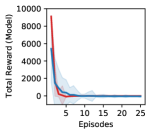
(c) Tabular

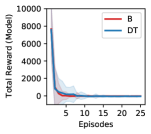
(d) State Aggregation

Figure H.4: The total reward obtained by the CIs of DT and B planning (a, b) on the SG environment and (c, d) in their corresponding models (learned on the SG environment) in the P&L setting with tabular and SA VE representations. Black & gray dashed lines indicate total reward obtained by the optimal & random policies, respectively. Shaded regions are one standard error over 100 runs.

H.1.3 TL Experiments

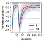
(a) State Aggregation

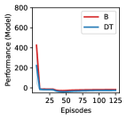
(b) Tabular

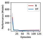
(c) State Aggregation

Figure H.5: The performance of the CIs of DT and B planning (a) on the SG environment and (b, c) in their corresponding models (learned on the SG environment) in the TL setting with tabular and SA VE representations. Black & gray dashed lines indicate the performance of the optimal & random policies, respectively. Shaded regions are one standard error over 100 runs.

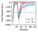
(a) Tabular

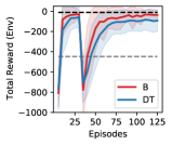
(b) State Aggregation

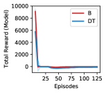
(c) Tabular

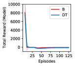
(d) State Aggregation

Figure H.6: The total reward obtained by the CIs of DT and B planning (a, b) on the SG environment and (c, d) in their corresponding models (learned on the SG environment) in the TL setting with tabular and SA VE representations. Black & gray dashed lines indicate total reward obtained by the optimal & random policies, respectively. Shaded regions are one standard error over 100 runs.

H.2 Experiments with MIs

H.2.1 P&L Experiments

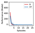
(a) Tabular

Figure H.7: The performance of the MIs of DT and B planning in their corresponding models (learned on the SG environment) in the P&L setting with tabular VE representations. Shaded regions are one standard error over 100 runs.

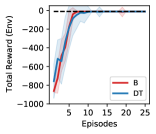
(a) Tabular

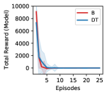
(b) Tabular

Figure H.8: The total reward obtained by the MIs of DT and B planning (a) on the SG environment and (b) in their corresponding models (learned on the SG environment) in the P&L setting with tabular VE representations. The black dashed line indicates the total reward obtained by the optimal policy. Shaded regions are one standard error over 100 runs.

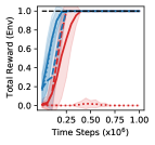
(a) Empty 10x10

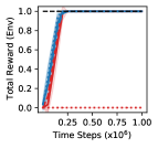
(b) FourRooms

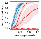
(c) SCS9N1

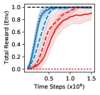
(d) LCS9N1

Figure H.9: The total reward obtained by the MIs of DT and B planning in the P&L setting with NN VE representations. The black dashed lines indicate the total reward obtained by the optimal policy in the corresponding environment. Shaded regions are one standard error over 50 runs.

H.2.2 TL Experiments

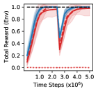
(a) RDS Sequential

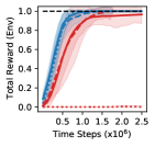
(b) RDS Train (0.35)

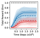
(c) RDS Test (0.25)

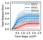
(d) RDS Test (0.35)

(e) RDS Test (0.45)

Figure H.10: The total reward obtained by the MIs of DT and B planning in the TL setting with NN VE representations. The black dashed lines indicate the total reward obtained by the optimal policy in the corresponding environment. Shaded regions are one standard error over 50 runs.

References

- Alver and Precup [2022] Safa Alver and Doina Precup. Constructing a good behavior basis for transfer using generalized policy updates. In International Conference on Learning Representations, 2022. URL https://openreview.net/forum?id=7IWGzQ6gZ1D.
- Anand et al. [2022] Ankesh Anand, Jacob C Walker, Yazhe Li, Eszter Vértes, Julian Schrittwieser, Sherjil Ozair, Theophane Weber, and Jessica B Hamrick. Procedural generalization by planning with self-supervised world models. In International Conference on Learning Representations, 2022. URL https://openreview.net/forum?id=FmBegXJToY.
- Arumugam et al. [2018] Dilip Arumugam, David Abel, Kavosh Asadi, Nakul Gopalan, Christopher Grimm, Jun Ki Lee, Lucas Lehnert, and Michael L Littman. Mitigating planner overfitting in model-based reinforcement learning. arXiv preprint arXiv:1812.01129, 2018.
- Barreto et al. [2017] André Barreto, Will Dabney, Rémi Munos, Jonathan J Hunt, Tom Schaul, Hado P van Hasselt, and David Silver. Successor features for transfer in reinforcement learning. Advances in neural information processing systems, 30, 2017.
- Barreto et al. [2019] André Barreto, Diana Borsa, Shaobo Hou, Gheorghe Comanici, Eser Aygün, Philippe Hamel, Daniel Toyama, Jonathan Hunt, Shibl Mourad, David Silver, et al. The option keyboard combining skills in reinforcement learning. In Proceedings of the 33rd International Conference on Neural Information Processing Systems, pages 13052–13062, 2019.
- Barreto et al. [2020] André Barreto, Shaobo Hou, Diana Borsa, David Silver, and Doina Precup. Fast reinforcement learning with generalized policy updates. Proceedings of the National Academy of Sciences, 117(48):30079–30087, 2020.
- Bertsekas [2021] Dimitri P Bertsekas. Rollout, policy iteration, and distributed reinforcement learning. Athena Scientific, 2021.
- Bertsekas and Tsitsiklis [1996] Dimitri P Bertsekas and John N Tsitsiklis. Neuro-dynamic programming. Athena Scientific, 1996.
- Campbell et al. [2002] Murray Campbell, A Joseph Hoane Jr, and Feng-hsiung Hsu. Deep blue. Artificial intelligence, 134(1-2):57–83, 2002.
- Chevalier-Boisvert et al. [2018] Maxime Chevalier-Boisvert, Lucas Willems, and Suman Pal. Minimalistic gridworld environment for openai gym. https://github.com/maximecb/gym-minigrid, 2018.
- Grimm et al. [2020] Christopher Grimm, Andre Barreto, Satinder Singh, and David Silver. The value equivalence principle for model-based reinforcement learning. In H. Larochelle, M. Ranzato, R. Hadsell, M.F. Balcan, and H. Lin, editors, Advances in Neural Information Processing Systems, volume 33, pages 5541–5552. Curran Associates, Inc., 2020. URL https://proceedings.neurips.cc/paper/2020/file/3bb585ea00014b0e3ebe4c6dd165a358-Paper.pdf.
- Grimm et al. [2021] Christopher Grimm, Andre Barreto, Gregory Farquhar, David Silver, and Satinder Singh. Proper value equivalence. In A. Beygelzimer, Y. Dauphin, P. Liang, and J. Wortman Vaughan, editors, Advances in Neural Information Processing Systems, 2021. URL https://openreview.net/forum?id=aXbuWbta0V8.
- Hafner et al. [2021] Danijar Hafner, Timothy P Lillicrap, Mohammad Norouzi, and Jimmy Ba. Mastering atari with discrete world models. In International Conference on Learning Representations, 2021. URL https://openreview.net/forum?id=0oabwyZbOu.
- Hamrick et al. [2021] Jessica B Hamrick, Abram L. Friesen, Feryal Behbahani, Arthur Guez, Fabio Viola, Sims Witherspoon, Thomas Anthony, Lars Holger Buesing, Petar Veličković, and Theophane Weber. On the role of planning in model-based deep reinforcement learning. In International Conference on Learning Representations, 2021. URL https://openreview.net/forum?id=IrM64DGB21.
- Jafferjee et al. [2020] Taher Jafferjee, Ehsan Imani, Erin Talvitie, Martha White, and Micheal Bowling. Hallucinating value: A pitfall of dyna-style planning with imperfect environment models. arXiv preprint arXiv:2006.04363, 2020.
- Jiang et al. [2015] Nan Jiang, Alex Kulesza, Satinder Singh, and Richard Lewis. The dependence of effective planning horizon on model accuracy. In Proceedings of the 2015 International Conference on Autonomous Agents and Multiagent Systems, pages 1181–1189. Citeseer, 2015.
- Kocsis and Szepesvári [2006] Levente Kocsis and Csaba Szepesvári. Bandit based monte-carlo planning. In European conference on machine learning, pages 282–293. Springer, 2006.
- Russell and Norvig [2002] Stuart Russell and Peter Norvig. Artificial intelligence: a modern approach. 2002.
- Schrittwieser et al. [2020] Julian Schrittwieser, Ioannis Antonoglou, Thomas Hubert, Karen Simonyan, Laurent Sifre, Simon Schmitt, Arthur Guez, Edward Lockhart, Demis Hassabis, Thore Graepel, et al. Mastering atari, go, chess and shogi by planning with a learned model. Nature, 588(7839):604–609, 2020.
- Silver et al. [2017] David Silver, Julian Schrittwieser, Karen Simonyan, Ioannis Antonoglou, Aja Huang, Arthur Guez, Thomas Hubert, Lucas Baker, Matthew Lai, Adrian Bolton, et al. Mastering the game of go without human knowledge. nature, 550(7676):354–359, 2017.
- Silver et al. [2018] David Silver, Thomas Hubert, Julian Schrittwieser, Ioannis Antonoglou, Matthew Lai, Arthur Guez, Marc Lanctot, Laurent Sifre, Dharshan Kumaran, Thore Graepel, et al. A general reinforcement learning algorithm that masters chess, shogi, and go through self-play. Science, 362(6419):1140–1144, 2018.
- Sutton [1990] Richard S Sutton. Integrated architectures for learning, planning, and reacting based on approximating dynamic programming. In Machine learning proceedings 1990, pages 216–224. Elsevier, 1990.
- Sutton [1991] Richard S Sutton. Dyna, an integrated architecture for learning, planning, and reacting. ACM Sigart Bulletin, 2(4):160–163, 1991.
- Sutton and Barto [2018] Richard S Sutton and Andrew G Barto. Reinforcement learning: An introduction. MIT press, 2018.
- Talvitie [2014] Erik Talvitie. Model regularization for stable sample rollouts. In UAI, pages 780–789, 2014.
- Taylor and Stone [2009] Matthew E Taylor and Peter Stone. Transfer learning for reinforcement learning domains: A survey. Journal of Machine Learning Research, 10(7), 2009.
- Tesauro [1994] Gerald Tesauro. Td-gammon, a self-teaching backgammon program, achieves master-level play. Neural computation, 6(2):215–219, 1994.
- Tesauro and Galperin [1996] Gerald Tesauro and Gregory Galperin. On-line policy improvement using monte-carlo search. Advances in Neural Information Processing Systems, 9:1068–1074, 1996.
- van Hasselt et al. [2019] Hado P van Hasselt, Matteo Hessel, and John Aslanides. When to use parametric models in reinforcement learning? Advances in Neural Information Processing Systems, 32:14322–14333, 2019.
- Van Seijen et al. [2020] Harm Van Seijen, Hadi Nekoei, Evan Racah, and Sarath Chandar. The loca regret: A consistent metric to evaluate model-based behavior in reinforcement learning. Advances in Neural Information Processing Systems, 33:6562–6572, 2020.
- Wang et al. [2019] Tingwu Wang, Xuchan Bao, Ignasi Clavera, Jerrick Hoang, Yeming Wen, Eric Langlois, Shunshi Zhang, Guodong Zhang, Pieter Abbeel, and Jimmy Ba. Benchmarking model-based reinforcement learning. arXiv preprint arXiv:1907.02057, 2019.
- Zhao et al. [2021] Mingde Zhao, Zhen Liu, Sitao Luan, Shuyuan Zhang, Doina Precup, and Yoshua Bengio. A consciousness-inspired planning agent for model-based reinforcement learning. Advances in Neural Information Processing Systems, 34, 2021.
- Łukasz Kaiser et al. [2020] Łukasz Kaiser, Mohammad Babaeizadeh, Piotr Miłos, Błażej Osiński, Roy H Campbell, Konrad Czechowski, Dumitru Erhan, Chelsea Finn, Piotr Kozakowski, Sergey Levine, Afroz Mohiuddin, Ryan Sepassi, George Tucker, and Henryk Michalewski. Model based reinforcement learning for atari. In International Conference on Learning Representations, 2020. URL https://openreview.net/forum?id=S1xCPJHtDB.