Optimal Parallel Sequential Change Detection under Generalized Performance Measures
Abstract
This paper considers the detection of change points in parallel data streams, a problem widely encountered when analyzing large-scale real-time streaming data. Each stream may have its own change point, at which its data has a distributional change. With sequentially observed data, a decision maker needs to declare whether changes have already occurred to the streams at each time point. Once a stream is declared to have changed, it is deactivated permanently so that its future data will no longer be collected. This is a compound decision problem in the sense that the decision maker may want to optimize certain compound performance metrics that concern all the streams as a whole. Thus, the decisions are not independent for different streams. Our contribution is three-fold. First, we propose a general framework for compound performance metrics that includes the ones considered in the existing works as special cases and introduces new ones that connect closely with the performance metrics for single-stream sequential change detection and large-scale hypothesis testing. Second, data-driven decision procedures are developed under this framework. Finally, optimality results are established for the proposed decision procedures. The proposed methods and theory are evaluated by simulation studies and a case study.
Keywords: Large-scale inference, multiple change detection, sequential analysis, multiple hypothesis testing
1 Introduction
Sequential change detection aims to detect distributional changes in sequentially observed data. Classical methods focusing on change detection in a single data stream have received wide applications in various fields, including engineering, education, medical diagnostics and finance [38, 32, 39, 37]. Several metrics have been proposed for evaluating their performance, under which optimality theory has been established [27, 33, 34, 31]; see [25, 36, 5] for a review.
The emergence of large-scale real-time streaming data has motivated multi-stream sequential change detection problems. One problem concerns detecting a common change shared by a subset of the streams [8, 10, 9, 29, 44, 20]. This problem is commonly seen in surveillance applications, where each data stream corresponds to a sensor, and the change point is caused by a failure in a subset of the sensors. A related problem, which has received much attention recently and will be the focus of the current work, considers a setting that each stream has its own change point [12, 13, 14, 11]. More specifically, a decision maker needs to declare whether a change has already occurred for each stream at each time point. Once a stream is declared to have changed, it is deactivated permanently so that its data is no longer collected. This problem will be referred to as a parallel sequential change detection problem.
The parallel sequential change detection problem is widely encountered in the real world. For example, [12, 24] consider an application to a multichannel dynamic spectrum access problem for cognitive radios. Each cognitive radio channel corresponds to a data stream, and the change corresponds to the time at which the primary user of the channel starts to transmit signals. A false discovery rate (FDR) is proposed to measure the proportion of false discoveries (i.e., unused channels) among the ones detected as occupied by primary users. [13, 14] consider monitoring an item pool for standardized educational testing. In this application, each stream corresponds to a test item that is reused in multiple test administrations, and the change point corresponds to the time at which the item is leaked to the public. A certain false non-discovery rate (FNR) is proposed to measure the proportion of leaked items among the non-detections (i.e., items that are not detected as having leaked). There are many other potential applications, such as the detection of credit card fraud [15], for which each stream corresponds to a credit card account, and the change point corresponds to a fraud event.
We note that it is often not a good idea to run a single-stream change detection procedure independently on individual streams. This is because the decision maker may want to control a certain compound risk that concerns all the streams as a whole, such as the FDR and FNR measures. Consequently, each decision at one time point requires all the up-to-date information from all the streams, making the parallel sequential change detection a challenge.
Several methods have been proposed in [12, 13, 14] to control the above compound risk measures in parallel sequential change detection problems. However, these methods, along with their theoretical properties, are established under relatively restrictive model assumptions and for specific risk measures. Specifically, [12] proposes a method based on the Benjamini-Hochberg method [6] for FDR control and establishes its asymptotic results. However, no results are given on the method’s optimality. Under a Bayesian setting, [13] and [14] propose methods for controlling a certain FNR measure at all time points. As shown in [13], under a geometric change point model and assuming the same pre- and post- change distribution for all the streams, this method maximizes the expected number of remaining streams at all time points while controlling the FNR to be no greater than a pre-specified tolerance level. However, it is unclear whether this optimality theory can be extended to more general models and other sensible risk measures.
The parallel sequential change detection problem is also closely related to the sequential multiple testing problem. The latter can be viewed as a special case when a stream can only change at the beginning of the process or never change. Several methods have been proposed for the sequential multiple testing problem, controlling compound risks. Specifically, [2], [3], and [41] consider controlling a familywise error rate, an FDR/FNR, and a generalized familywise error rate, respectively. While the risk measures may be relevant, their methods and theoretical results can hardly be extended to the current change detection problem.
This work provides a unified decision theory framework for parallel sequential change detection problems under general classes of change point models and performance measures. A computationally efficient sequential method is developed under the proposed framework. Two optimality criteria are introduced, for which the proposed method is shown to be optimal under suitable conditions.
Our contributions are summarized below:
-
•
We propose a general class of performance metrics to evaluate the sequence procedures. This class of metrics not only includes existing metrics as special cases (e.g., FDR [12] and the local FNR metric [13]) but also introduces new metrics that are closely related to the metrics for single-stream change detection and multiple hypothesis testing. See Section 2.4 and Section 4.3 for more examples.
-
•
We propose a sequential procedure (Algorithms 1–4) that is easy-to-implement and is data-driven. It automatically adapts to various model settings when controlling the risk measures to a pre-specified tolerance level, without requiring additional Monte Carlo simulation or bisection search commonly used in sequential problems to determine decision boundaries (see, e.g., [4]).
-
•
We provide two optimality criteria for the parallel sequential change detection problem, including the local and uniform optimalities. The local optimality concerns the maximization of a utility measure in the next step, and uniform optimality refers to the maximization of the utility measure at all time. We show that the proposed method is locally optimal under very mild conditions and uniformly optimal under stronger conditions (Theorems 1–3).
We note that the precise characterization of the conditions for uniform optimality requires the analysis of stochastic processes on a special non-Euclidean space. To this end, we develop new analytical tools for comparing vectors and stochastic processes with different dimensions, possibly due to early stopping. This analytical tool may be useful in the theoretical analysis of other sequential decision problems.
The remainder of the paper is organized as follows. In Section 2, we describe the change point models, the class of parallel sequential change detection methods, a general class of performance metrics, and the optimality criteria. We also provide examples of generalized performance metrics. In Section 3, we propose a parallel change detection method (Algorithms 1 and 2) and provide a simplified version of this method under mild conditions on the performance measures (Algorithms 3 and 4). Section 4 provides theoretical results for the proposed methods including their optimality properties and the connection with recent works. In Sections 5 and 6, we evaluate the performance of the proposed method through simulation studies and a case study. Concluding remarks and future directions are given in Section 7. For space reasons, all the proofs of the theoretical results and part of the simulation results are postponed to the Appendix in the supplementary material.
2 Problem Setup
2.1 Model Assumptions
Consider the case where there are data streams, and let denote the set . At each time epoch , an observation is obtained from the th data stream, for . Each data stream is associated with a change point for . Under a Bayesian parallel change point model, the change points are assumed to be independent and identically distributed (i.i.d.) with
| (1) |
for and . Given , are independent for , and have conditional density
| (2) |
with respect to some baseline measure. That is, are independent given the change points, and follow pre- and post- change density functions and , respectively. In particular, corresponds to the case where the change point never occurs to the th stream. That is, follows the pre-change density function for all .
2.2 Parallel Sequential Change Detection Procedures
A decision maker sequentially observes data from the parallel data streams and determines whether change points have already occurred to these data streams at each time. Once a change point is declared, the corresponding data stream is deactivated and its data are no longer collected. This decision process is characterized by an index set process for , where if and only if the decision maker has not declared a change in the th stream at time yet (i.e., stream is active at time ). Specifically, the available information at time is contained in the historical data and, equivalently, the induced information -field . At each time , the decision maker selects the index set based on the current information . That is, is measurable with respect to . Denote by the set of all such compound sequential decisions. A graphical illustration of the decision process is given in Figure 1.
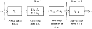
We make a few remarks on the information filtration and the decision process. First, we require , meaning that all the streams are initially active and data from all the streams are collected at time . Second, is measurable with respect to , meaning that the decision history is tracked in the current information. Third, is measurable with respect to , indicating that is observed if and only if stream is active at time and (i.e., ). Fourth, is required to be measurable with respect to , meaning that the decision maker selects the active streams for time based on all the information available at time . Lastly, is required to be a subset of for all , meaning that the deactivation of streams is permanent. That is, no future data will be collected at a stream, once a change is declared at that stream.
Remark 1.
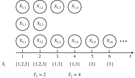
Although described in a different way, the class of sequential decisions defined above is equivalent to that in [12]. In [12], a parallel sequential procedure is defined through a sequence of stopping times along with a sequence of index sets . At each stopping time , a decision maker declares change points for streams in and exclude those streams from the future decision process. Then, the sequences and can be represented using the sequence as and where , . An example where is given in Figure 2 for a graphical illustration.
Another way to understand a compound sequential change detection procedure is to view it as a sequence of mappings , where each determines according to the historical information . That is, is a measurable function with respect to and satisfying that for all .
2.3 Generalized Performance Measures and Optimality Criteria
Ideally, a perfect sequential change detection procedure collects all the pre-change streams in the set at each time point (i.e., ). However, this is not achievable by any sequential decision because s are unobserved. To this end, we consider a general class of performance measures to compare the performance of different sequential decisions. We assume each sequential decision is associated with a risk process, denoted by , and a utility process, denoted by . The risk process is used to quantify the loss of a sequential decision at time due to the false detections of pre-change streams and/or the non-detection of post-change streams, while the utility process is used to reward the correct decisions. Our goal is to find a good sequential decision that has a relatively small and a relatively large at every time point. Below, we first give formal statements of the optimality criteria, and then introduce several examples of and in Section 2.4, followed by additional discussions.
Let
| (3) |
be the posterior probability that the change point has already occurred at time for the -th stream given the information up to time . Under the Bayesian setting, is also the best estimator (under the squared error loss) of , where denotes the indicator function. A simple iterative updating rule is derived to calculate at each time, which will be discussed in Section 3.
Throughout the paper, we consider risk and utility processes that are functions of . That is, there are pre-specified functions and such that
| (4) |
and
| (5) |
Let denote a pre-specified tolerance level, and let
where denotes the risk process associated with the sequential decision , and denotes the entire set of parallel sequential detection procedures described in Section 2.2. The set collects all sequential decisions that control the risk process to be no greater than the tolerance level at all time points.
We note that risk process is an adaptive stochastic process with respect to the information filtration . It is easy to verify that for . That is, the expected risk is also controlled below or equal to the same tolerance level. In addition, any weighted average of across different time points are also controlled. We provide additional discussion and theoretical results regarding this point in Section 4.3.
The following regularity assumptions over the risk and utility functions are imposed throughout the paper.
Assumption 1.
For any and , . In addition, the utility function is bounded at each time .
The assumption on guarantees that the class of sequential decisions controlling the risk process at a pre-specified level is non-empty, i.e., . The boundedness assumption on is a mild condition to ensure the integrability of the utility process.
Given a pre-specified tolerance level and sequences of functions and , we define two optimality criteria for sequential decisions in .
Definition 1 (Uniform Optimality).
A sequential decision is called uniformly optimal if
for all , where and denote the utility process associated with sequential decisions and , respectively.
Definition 2 (Local Optimality).
A sequential decision is called locally optimal at time , if
for any satisfying , for .
We make a few remarks on the above optimality criteria. First, in most applications, there is a trade-off between minimizing the risk and maximizing the utility. That is, a sequential decision that has relatively small risk tends to have relatively small utility at the same time. Thus, we define both uniform and local optimality through constrained optimization problems, where the overall goal is to find a sequential decision so that its corresponding risk process is controlled to be no greater than the tolerance level while the expected utility is no less than any other sequential decisions that control the risk process at the same level. Second, a uniformly optimal sequential decision has the largest expected utility among all decisions in at every time point. In contrast, a locally optimal sequential decision only has the largest expected utility at a given time point given the decisions at previous time points. Thus, uniform optimality is a stronger notion than local optimality. A sequential decision that is locally optimal at every time point does not necessarily imply that it is also uniformly optimal. In later sections, we show that locally optimal sequential decisions exist under very weak assumptions on the risk and utility measures, while uniformly optimal sequential decisions only exist under stronger assumptions of the change point model and the performance measures. Third, we assume the same tolerance level for every time for ease of presentation. Our methods and theory can be easily extended to the class of sequential decisions whose risk is controlled at different levels at different time points. That is, for a sequence of constants . We can see this by redefining the risk process as and replacing by .
2.4 Examples of Generalized Performance Measures
We start with several examples of performance measures in the forms of (4) and (5), which are motivated by common risk measures in the literature of multiple hypotheses testing [17, 19, 18, 6]. All of the risk measures discussed in this section satisfy Assumption 1 for .
For the consistency of notation, the sum over an empty set is defined to be (i.e., ), and the product over an empty set is defined to be (i.e., ).
Example 1 (Local family-wise error rate (LFWER)).
Consider the event
| (6) |
which happens when at least one false non-detection occurs at time . Because is not directly observed, we consider the its posterior probability given the information up to time ,
| (7) |
Example 2 (Generalized local family-wise error rate (GLFWER)).
Given , we consider the event
| (8) |
This event happens when false non-detections occur in at least data streams. Its posterior probability given information up to time is
| (9) | ||||
| (10) |
In addition, if .
Comparing (7) with (9), we can see that GLFWER extends LFWER by allowing for more false non-detections. Under a large-scale setting with many data streams, it may be more sensible to use GLFWER with its value chosen based on the total number of streams to achieve a balance between false detections and false non-detections. Similar risk measures have been proposed for sequential multiple testing [41].
Example 3 (Local false non-discovery rate (LFNR)).
Local false non-discovery rate (LFNR) is defined in [13], which extends the concept of LFNR in multiple testing to parallel sequential change detection. It is defined as follows. First, the false non-discovery proportion (FNP) is defined as
| (11) |
FNP describes the proportion of post-change streams among the active ones. Then, the local false non-discovery rate (LFNR) at time is defined as the Bayes estimator (i.e., posterior mean) of given information up to time . That is,
| (12) |
Compared with LFWER and GLFWER, LFNR depends on s in a linear rather than multivariate polynomial form. In addition, LFNR is scalable under a large-scale setting in the sense that the same tolerance level can be used as grows large.
Example 4 (Local False Discovery Rate (LFDR)).
Similar to LFNR, LFDR also has the appealing feature of scalability for large . The difference between LFNR and LFDR lies in whether focusing on false detections or false non-detections.
In [12], an aggregated version of false discovery rate (AFDR)111In [12], this risk measure is referred to as ‘false discovery rate (FDR)’. Here, we name it as AFDR to distinguish it from LFDR. is considered, which can be viewed as the expectation of a weighted average of LFDR at different time points. More discussions on the connection between LFDR and AFDR will be provided in Section 4.
Next, we provide two examples of performance measures motivated by single-stream sequential change detection. Denote by the detection time of the th stream,
| (15) |
Note that plays a similar role as the stopping time in the standard single-stream sequential change detection problem. Indeed, is a stopping time with respect to for all .
Example 5 (Incremental Average Run Length (IARL)).
We define the incremental run length (IRL) aggregated over different streams as
| (16) |
IRL indicates the total number of pre-change streams being used at a given time. We refer to its posterior mean as the incremental average run length (IARL), defined as
| (17) |
where
| (18) |
IRL and IARL are closely related to the average run length to false alarm (ARL2FA) that is commonly used to measure the propensity for making a false detection in a single-stream sequential change detection problem. Specifically, taking summation of over , we obtain
| (19) |
which is the total run length from different data streams up to the change point by time . Moreover, we have
| (20) |
Thus, the sum of the expected value of IARL across time leads to the total averaged run length up to the change point.
Example 6 (Incremental Average Detection Delay (IADD)).
We define the incremental detection delay (IDD) aggregated over all the streams as
| (21) |
IDD counts the total number of post-change streams that are active at a given time. We refer to its posterior mean as the incremental average detection delay (IADD), defined as
| (22) |
IDD and IADD are incremental-and-compound versions of detection delay and average detection delay (ADD), which are commonly used to measure false non-detection in single-stream sequential change detection [43]. Specifically, by taking summation over , we have
| (23) |
and
| (24) |
Among the above examples, LFWER, GLFWER, and LFNR are error rates for false non-detections, LFDR is an error rate for false detections, IARL estimates the number of pre-change streams that are active, and IADD estimates the number of post-change and active streams. Because a small value of LFWER (or GLFWER/LFNR/IADD) and a large value of IARL (or minus LFDR) is desired, we could choose the risk process and the utility process , or and . Note that in the above examples, there is a trade-off between and . That is, if one declares detection at more data streams, then the corresponding LFWER, GLFWER, LFNR, and IADD tend to be smaller and IARL and minus LFDR tend to be smaller as well. Thus, the optimality criteria (Definitions 1 and 2) formulated through constrained optimization are reasonable.
The choices of and should be application-driven. In practice, we suggest to choose the risk process with a known range so that the tolerance level is easy to specify. For example, LFWER, GLFWER, LFNR, and LFDR represent certain probability/expected proportions that are known to be between . Thus, they are sensible choices of , for which setting the tolerance level is relatively straightforward.
3 Proposed Sequential Decision Procedures
In this section, we first provide a formula for computing the posterior probability , which is a key quantity in computing the risk and utility measures. Then, we present our proposed sequential decisions for controlling the risk process at a given level, followed by a simplified version of the algorithm to reduce the computational complexity.
3.1 Recursive Formula for
Recall and . Let
| (25) |
Given and , can be computed using the recursive formula
| (26) |
where we define . Then, we obtain
| (27) |
3.2 Proposed Sequential Decision for Unstructured Risk and Utility
We first propose a one-step selection rule to select , given and so that the risk is controlled to be no greater than . This one-step selection rule goes over all possible subsets of , and then select the one which attains the highest utility . Algorithm 1 implements this idea.
According to Assumption 1, . Thus, in line 3 of the above algorithm is well-defined. The next proposition states that the above one-step selection rule can control the risk process at any given level.
Note that Proposition 1 does not require any assumptions on and except for Assumption 1, which ensures the existence of the set in the last line of Algorithm 1.
Next, we combine Algorithm 1 at different time points to obtain a sequential decision in . At each time , this sequential decision selects using Algorithm 1 and deactivates data streams that are not in the index set. Algorithm 2 below implements this idea.
3.3 Simplified Sequential Decision for ‘Monotone’ Risk
At each time , directly applying Algorithm 1 requires evaluating and comparing the risk and utility associated with subsets, which is computationally intensive when is large. In many cases where the risk and utility satisfy additional monotonicity assumptions, this algorithm can be simplified, reducing the computational complexity significantly. In this section, we provide one such assumption, under which the proposed sequential decision only requires evaluating and comparing the risks associated with subsets.
Assumption 2.
For all non-empty , , , , and , we have and .
Under Assumption 2, tends to become larger and tends to become smaller if we keep streams with relatively smaller posterior probability active. Under this assumption, Algorithm 1 can be simplified to the following Algorithm 3, and it also controls to be below a pre-specified level . As will be discussed in Corollary 1, all the risk and utility measures presented in Examples 1 – 6 satisfy this assumption.
The following Algorithm 3 selects so that streams with relatively large posterior probabilities are detected and those with relatively small posterior probabilities are kept active. The cut-off point for the detection is decided by maximizing the utility while controlling the risk at time . Because Algorithm 3 restricts to be a subset of streams with relatively small posterior probability, it only involves evaluating and comparing the risk and utility functions associated with subsets, and, thus, reduces the computational complexity to the order .
Note that under Assumption 1, . Thus, the forth line of the above Algorithm 3 is well-defined. The following Algorithm 4 gives an overall sequential decision rule by adopting Algorithm 3 at every time point.
4 Theoretical Properties of Proposed Methods
In this section, we first show that the proposed sequential decision is locally optimal under very weak assumptions in Section 4.1. Then, we show that the simplified sequential decision is uniformly optimal under stronger model assumptions and additional monotonicity assumptions on risk and utility measures in Section 4.2. We also provide theoretical results on aggregated risk and utility measures of the proposed methods in Section 4.3.
4.1 Local Optimality Results
The following two theorems show that the proposed sequential decision is locally optimal under Assumption 1 while is locally optimal under Assumptions 1 and 2. That is, they satisfy Definition 2.
Theorem 2.
The next corollary applies the above results to examples given in Section 2.4.
Corollary 1.
If and , , or and , then the simplified sequential decision is locally optimal.
If and and , then the simplified sequential decision is locally optimal.
4.2 Uniform Optimality Results
In this section, we show that the proposed sequential decision rule defined in Algorithm 4 is uniformly optimal under stronger assumptions. We note that the uniform optimality results developed in the current work are non-trivial extensions of those in [13]. In particular, we consider a general class of risk and utility measures while [13] only allows the risk measure to be LFNR. Moreover, time-heterogeneous pre/post- change distributions and non-geometric priors for the change points are allowed in the current work. These extensions require a delicate analysis of a special class of monotone functions and stochastic processes defined over a non-Euclidean space.
The assumptions for establishing the uniform optimality results include monotonicity assumptions on the risk and utility processes and assumptions on the pre- and post- change distributions. We point out that the monotonicity assumptions are made on functions over a special non-Euclidean space
| (28) |
which contains ordered vectors of different dimensions. Thus, the definition of monotonicity is non-standard.
Specifically, for functions maps to , we define two types of monotonicity.
Definition 3 (Entrywise increasing functions).
A function is “entrywise increasing”, if for all , , satisfying for . In addition, a function is “entrywise decreasing” if is “entrywise increasing”.
Definition 4 (Appending increasing functions).
A function is “appending increasing”, if for all , , , for all . In addition, for .
For each vector , denote its order statistic by . That is, is a permutation of satisfying . We can see that if for all , then .
Assumption 3.
There exists a measurable function such that . In addition, is entrywise increasing and appending increasing.
Assumption 4.
There exists a measurable function such that . In addition, is entrywise decreasing and appending increasing.
Assumption 5.
The pre- and post-change distributions and are the same for different . That is, and for all .
Theorem 3.
Proof.
The proof is involved that requires monotone coupling for stochastic processes living on the space . It is given in Appendix D. ∎
We make several remarks on the above theorem. First, under Assumptions 3 and 4, risk and utility measures are symmetric functions . These assumptions rule out the cases (e.g., LFDR defined in Example 4) where the risk also depends on s for , without which the uniform optimal solution may not exist (see Counterexample 1 below). Second, under the monotonicity assumptions that s are entrywise increasing, the risk process tends to be larger if the posterior probability of the change points associated with the selected streams is larger. It is also appending increasing, meaning that the risk tends to be larger if more streams are kept active. Similarly, the utility process tends to be larger if fewer streams are kept active and the posterior probabilities associated with the selected streams are smaller. Third, we require the pre- and post- stream distributions and to be identical for different streams. In this case, the process has identical distribution for different and contributed in a symmetric way to the risk and utility processes.
For most of applications, it is easy to check Assumptions 1 and 5. In some cases, additional efforts are needed to verify monotonicity assumptions described in Assumptions 3 and 4. Below we provide sufficient conditions for the monotonicity conditions. Note that the risk and utility measures described in Examples 1, 2, 3, 5, and 6 are all symmetric multivariate polynomials of the posterior probabilities. Thus, we restrict the analysis to the polynomial case in the next proposition.
Proposition 4 (Polynomial case).
Let be a function in the following form
| (29) |
Note that . If satisfies
| (30) |
where and denotes the dimensional vector whose first elements are and last elements are all , then is entrywise increasing.
Remark 2.
Now we apply the uniform optimality result in Theorem 3 to performance measures described in Examples 1, 2, 3 and 5.
Corollary 2.
If , , and , then under Assumption 5, is uniformly optimal.
We point out that described in Example 4 does not satisfy the assumptions made in Theorem 3. Thus, we do not have uniform optimality results for it. Indeed, if , then the uniformly optimal sequential decision may not exist. A counterexample is given below.
Counterexample 1.
Let , , , and for , , , and . That is, the pre- and post- change distributions are Bernoulli distributions with parameters and , respectively, and s are uniformly distributed over . We further assume that the tolerance level , the risk process (see Example 4) and the utility process (see Example 6).
In this setting, there does not exist a sequential decision achieving the maximum of the expected utility at both times and . This implies that there is no uniformly optimal sequential decision. We leave detailed calculation in Appendix D.
4.3 Implications on Aggregated Risk
Let be a sequence of non-negative random variables satisfying , and be a sequence of non-negative constants. Consider the following aggregated risk (AR) and aggregated utility (AU),
| (34) |
The aggregated risk and utility metrics defined above provide a summary of the performance across time. These types of risk and utility measures are considered in many recent works on multi-stream sequential change detection and hypothesis testing, including [3, 41, 40, 12].
The next proposition shows that if the risk process is controlled at the desired tolerance level at every time point, then the aggregated risk is also controlled at the same level.
Proposition 5.
Let and be the corresponding aggregated risk defined in (34). Then,
Note that the reverse statement does not hold. That is, the aggregated risk being controlled does not imply the risk at each time being controlled.
The next proposition shows that a uniformly optimal sequential decision also maximizes the aggregated utility.
Proposition 6.
Suppose that is uniformly optimal in . Then, for the aggregated utility defined in (34),
where and denote the aggregated utility associated with and , respectively.
Next, we use Propositions 5 and 6 to make a connection between the current results and recent works on the sequential multiple testing and parallel sequential change detection [40, 12, 13].
4.3.1 Controlling generalized error rates in multi-stream sequential hypothesis testing
Note that if (i.e., change points either occur at the beginning or never occur), the sequential change point detection problem reduces to a sequential multiple hypotheses testing problem, where the goal is to choose between and for ,
under a Bayesian setting, where and . In addition, we assume that are jointly independent.
Let . We define the generalized family-wise error rate (GFWER) as
| (35) |
where is a stopping time and the event is defined in (8). can be viewed as a generalized family-wise error rate measuring type-II errors in sequential multiple hypotheses testing, which takes a similar form as the generalized type-II error rate in [40, 41, 1, 2]. Specifically, if we reject at time if and only if . Then,
in the context of multiple hypotheses testing.
The next corollary of Proposition 5 shows that the proposed method controls the GFWER in the perspective of the hypothesis testing problem.
Corollary 3.
Note that the above Corollary 3 holds for any stopping time . In particular, if we let grow to infinity, then Corollary 3 states that the GFWER accumulated over all the time points is controlled to be no greater than . If we let as defined in Remark 1, then different data streams are stopped at the same detection time . In this case, the proposed sequential procedure belongs to the class of sequential multiple testing procedures described in [41].
4.3.2 Controlling aggregated false discovery rate
The aggregated false discovery rate (AFDR) is considered in [12],
| AFDR | (36) |
where is a positive integer that is referred to as a ‘deadline’. The next proposition states that any decision that controls at every time also controls AFDR asymptotically.
Proposition 7.
Let and . Assume that there exist a sequence of constants and a sequence of random variables such that converges to in probability and converges to in probability for all as grows to infinity. Then, . That is, AFDR is controlled to be no greater than asymptotically.
4.3.3 Maximizing total average run length
Let the total average run length (TARL) be
| (37) |
where is defined in (15). TARL aggregates IRLt across different time points, and can be viewed as an extension of the classic ARL2FA to multi-stream problems. The next corollary of Proposition 6 shows that the proposed method also maximizes TARL under certain conditions.
5 A Simulation Study
In this section, we study the performance of the proposed sequential decision defined in Algorithm 4 through a simulation study. We choose and in the simulation study and let the tolerance level . We also compare the performance of the proposed method with the MD-FDR method proposed in [12].
We also conduct a simulation study where . For space reason, we leave it to the appendix in the supplementary materials.
We let and for all and . In addition, let , and for . That is, we set the pre- and post-change probability distributions to be the Gaussian distributions and , respectively, and set the prior distribution for the change point to be a mixture of a point mass at infinity and a geometric distribution.
We assess and compare the performance of two sequential decisions. The first sequential decision is the the proposed method described in Algorithm 4 with (defined in Example 4) and (defined in Example 6). With this choice of and , line 4 in Algorithm 3 can be simplified as
The other sequential decision is the MD-FDR method developed in [12]. Following the MD-FDR method, the risk measure AFDR defined in (36) is guaranteed to be no greater than the tolerance level .
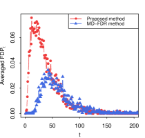
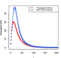
We first compare the proposed method with the MD-FDR method in terms of their FDPt (defined in (13)) and (defined in (21)) for fixed with independent Monte Carlo simulations. The averaged and across the replications are plotted in Figures 3 and 4 as functions of . According to Figure 3, the averaged of both methods are below for all with a trend of first increasing and then decreasing as increases. The of the proposed method has a plateau near for . In addition, the of the proposed method is larger than that of the MD-FDR method, which suggests that the proposed method is less conservative while still controlled under the target tolerance level. Figure 4 compares the averaged of the proposed method and the MD-FDR method for different . It displays that, for both methods, first increases and then decreases as increases. The proposed method has a lower averaged than the MD-FDR method for all , indicating a smaller detection delay.
Next, we compare the two methods in terms of aggregated performance measures. In particular, we consider the aggregated risk AFDR defined in (36), where we set the deadline parameter . For aggregated utility, we consider the the total average detection delay (TADD), defined as
| (38) |
where is defined in (23). Then, we let the aggregated utility be . A higher utility, which corresponds to a lower TADD, reflects a quicker detection of the changes.
Tables 1 and 2 compare the two methods in terms of their aggregated risk AFDR and the aggregated utility TADD, respectively, which are estimated based on a Monte Carlo simulation with 1000 replications. From Table 1, we can see that both the proposed method and MD-FDR method control AFDR below the tolerance level , while the MD-FDR method is more conservative. We also note that as grows larger, AFDR of the proposed method is approaching . From Table 2, we can see that the TADD of the proposed method is significantly less than that of the MD-FDR method, indicating that the proposed method detects changes faster than the MD-FDR method, when the AFDR of both methods are controlled at the same level. An interesting observation is that TADD of both methods scale with as grows. That is, seems to converge to a constant as grows large. Specifically, for the proposed method, is around . For the MD-FDR method, is around for large .
Overall, these results suggests that the proposed method is less conservative and adapts better to the tolerance level than the MD-FDR method.
| K | Proposed method | MD FDR method |
|---|---|---|
| 10 | () | ( |
| 100 | () | () |
| 200 | () | () |
| 500 | () | () |
| 1000 | () | () |
| K | Proposed method | MD FDR method |
|---|---|---|
| 10 | 45.8 (0.5) | 61.4 (0.5) |
| 100 | 413.8 (1.3) | 650 (1.7) |
| 200 | 799.8 (1.9) | 1304.1 (2.4) |
| 500 | 1964.9 (3.0) | 3264 (3.7) |
| 1000 | 3891.4 (4.0) | 6535.3 (5.2) |
6 A Case Study: Multi-Channel Spectrum Sensing in Cognitive Radios
In this section, we conduct a case study on a multi-channel spectrum sensing problem for cognitive radios, following the settings described in [12]. Cognitive radios are radios that can dynamically and automatically adjust their operational parameters according to the environment so that the spectrum is utilized more efficiently [22, 30]. To make the most out of a spectrum, a cognitive user is allowed to use the idle spectrum band when the primary user is not transmitting. However, when the primary user starts transmission, the cognitive user should detect the change and vacate the spectrum band as soon as possible. The detection of the transmission of the primary user can be formulated as a sequential change detection problem, where the transmission time corresponds to the change point [24, 12].
We consider a multi-channel spectrum sensing problem for cognitive radios, where there are independent frequency channels assigned to independent primary users. The cognitive users monitor the spectrum bands and collect signal samples sequentially. The distribution of the signals will change when a primary user starts transmission. As soon as the change is detected, the cognitive user vacates the spectrum band, so that the primary user can use it without interference. Here, each channel corresponds to a data stream, and the time that a primary user starts transmission corresponds to a change point in that data stream. Our goal is to have a sequential decision that can detect the transmission of the primary user at each channel quickly to reduce the interference, while controlling the false discovery rate, which corresponds to the expected proportion of unoccupied channels among the detected ones.
Specifically, we assume that is the signal collected from the th cognitive user at time , is the time when the -th primary user starts transmission, and s and s follow the change point model described in (1) and (2). For the change point , we further assume that
with and . That is, follows a mixture distribution of a point mass at infinity and a geometric distribution.
For the pre- and post- change distributions, we assume
where denotes a Gaussian white noise and denotes the faded received primary radio signal at the cognitive user’s end. We further assume that , , and s and s are independent, where and denote the circularly-symmetric complex Gaussian distributions with mean and the complex variance and , respectively. Note that a complex random variable has a circularly-symmetric complex Gaussian distribution with a variance if its real and imaginary parts are independent and identically distributed univariate Gaussian random variables with the mean zero and the variance .
Under this model, has the distribution
Notice that in this setting, the streams share the same pre-change distribution, but have different post-change distributions characterized by their different variances. The above distribution assumptions are commonly adopted in the literature [24, 12].
In this case study, we assume and sample independent s from a uniform distribution over . We then treat as known parameters. Here, we sample from an interval to mimic the practical situation where the signals sent by the primary users may experience channel attenuation at the cognitive user’s end, which results in a range of variance-distinct post-change signals.
Let the tolerance level . We compare the performance of the proposed sequential decision following Algorithm 3 (with and ) and the MD-FDR method proposed in [12]. We also consider the aggregated risks AFDR (defined in (36)) and the aggregated utility TADD (defined in (38)).
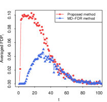
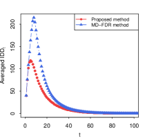
Figures 5 and 6 show the averaged and for different based on a Monte Carlo simulation with 1000 replications. We see that of both methods are below 0.1 with a peak at around and , respectively. According to Figure 5, the averaged of the MD-FDR method appears to be smaller than that of the proposed method for time , while both of them decline at a similar rate after time . For larger , the averaged of both methods are close to zero. According to Figure 6, the averaged of the MD-FDR method is larger than that of the proposed method for all , which suggests that the proposed method detects changes more quickly than that of the MD-FDR method.
Tables 3 and 4 show the AFDR and TADD for both methods for . According to the tables, the AFDR of both methods are controlled to be less than , with the AFDR of the MD-FDR method smaller than that of the proposed method for all . This indicates that the proposed method is less conservative in controlling FDR-type of risks, when compared with the MD-FDR method. Moreover, the proposed method has a much smaller TADD that that of the MD-FDR method for all , indicating that the proposed method has a smaller detection delay.
| K | Proposed method | MD FDR method |
|---|---|---|
| 10 | () | () |
| 100 | () | () |
| 200 | () | () |
| 500 | () | () |
| 1000 | () | () |
| K | Proposed method | MD FDR method |
|---|---|---|
| 10 | 122.1 (1.2) | 162 (1.4) |
| 100 | 1115.8 (3.7) | 1708.5 (4.6) |
| 200 | 2178.2 (5.1) | 3434.8 (6.6) |
| 500 | 5293.4 (8.1) | 8609.4 (10.4) |
| 1000 | 10460.1 (11.3) | 17246.7 (14.8) |
7 Conclusions
The parallel sequential change detection problem is widely encountered in the analysis of large-scale real-time streaming data. This study introduces a general decision theory framework for this problem, covering many compound performance metrics. It further proposes a sequential procedure under this general framework and proves its optimal properties under reasonable conditions. Simulation and case studies evaluate the performance of the proposed method and compare it with the method proposed in [12]. The results support the theoretical developments and also show that the proposed method outperforms in our simulation studies and case study.
The current study can be extended in several directions. First, the current parallel sequential change detection framework may be extended to account for multiple types of decisions, including alerting the changes without stopping the streams and diagnosis of the post-change distribution upon stopping, which is also known as the sequential change diagnosis [28, 16]. Second, in many applications, the post-change distribution of data is challenging to obtain. Also, it is sometimes difficult to specify a prior distribution for the change points. In these cases, it is desirable to formulate the problem in a non-Bayesian decision theory framework, and develop a flexible parallel sequential change detection method that is robust for unknown post-change distributions under this framework. Third, we assume that the change points are independent for different data streams. For some applications, it is reasonable to extend the methods to the case where the change points are dependent. For example, the change points may be driven by the same event [44] or propagated by each other [45].
Appendix
Appendix A An additional simulation study
In this simulation study, we let and for all and and , and for . In addition, we set and consider the risk process (see Example 3) and the utility process (see Example 5).
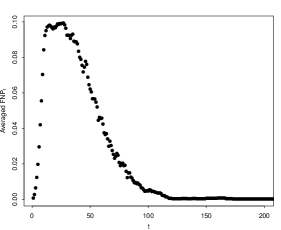
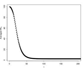
We plot the averaged risk measure and the averaged utility measure of the proposed method defined in Algorithm 4 in Figures 7 and 8 based on a Monte Carlo simulation with 1000 replications. From Figure 7 we can see that the averaged is below 0.1 with a peak at around , which is consistent with Proposition 3. From Figure 8 we can see that is decreasing to as increases.
Appendix B Proof of Results in Section 3
Proof of Proposition 1.
Proof of Proposition 2.
Appendix C Proof of Results in Section 4.1
Proof of Theorem 1.
First, we know that according to Proposition 2.
Next, we compare the proposed sequential decision with an arbitrary sequential decision satisfying , for . Let be the index set of active streams following at all time points, and be the set selected by at time . Note that both and select as the index sets at time , according to the assumption that for .
According to the second and third line of Algorithm 1, satisfies subject to . Because , and the index set selected by and at time are both , we have a.s. This further implies That is, . The proof is completed by taking expectation on both sides. ∎
Proof of Theorem 2.
First, according to Theorem 1, the sequential decision obtained from Algorithm 2 is locally optimal. Thus, to show obtained from Algorithm 4 is also locally optimal, it suffices to show that is a special case of under Assumption 2. Let be the index set of active streams following the decision at every time. For each , it is sufficient to show that obtained in the forth line of Algorithm 3 also solves the optimization problem in the third line of Algorithm 1. To see this, it is sufficient to show
| (39) |
for any set satisfying .
Recall that are chosen so that . We discuss two cases: for some ; and for all . In what follows, we show that (39) holds for both cases.
Case 1: for some .
In this case, . Recall that obtained in the forth line of Algorithm 3 satisfies . Thus, We complete the proof of (39) in Case 1 by recalling that and .
Case 2: for all .
Let . In this case, there exists and such that (we set for the ease of presentation).
Note that , , and . According to Assumption 2, we have
| (40) |
That is, the risk evaluated at is no greater than at . With similar arguments, we have
| (41) |
Combining (40) and (41), we obtain
| (42) |
Recall that . Thus, the above inequality also implies
| (43) |
Next, we consider . By replacing with and ‘’ with ‘’ in (40) – (42), we obtain under Assumption 2. This implies According to equation (43) and the proof in Case 1, we have Combining these inequalities, we obtain (39). ∎
Proof of Corollary 1.
We start with the proof of the first statement of the corollary. According to (7) – (22), we have if , and if . In addition, according to the definition, , and fall into the interval , and and belong to . Thus, Assumption 1 is verified for .
Next, we show that if and then Assumption 2 is satisfied. Without loss of generality, we assume , where . Also, assume , , , and . We consider different choices of and below.
Lemma 1.
For , then
if for all .
We apply the above lemma with , and . Since we obtain
It follows that
If , we have
If , we have
If , then where we used the fact that .
If , then .
Since is a special case of where in Example 2, if , we also have . The proof for the other set of and can be obtained similarly by flipping their signs. We omit the repetitive details. ∎
Appendix D Proof of Results in Section 4.2
D.1 Proof sketch for Theorem 3
The proof of Theorem 3 is involved. In this section, we provide a high level summary of steps in proving Theorem 3 and an overview of the supporting lemmas in Appendix D.2–D.4. We will wrap up these supporting results and provide the proof of Theorem 3 in Appendix D.5.
In Appendix D.2, we define a special partial order relationship ‘’ over the space so that one can compare vectors in even when they have different dimensions. We also study monotone functions in terms of this special partial order relation. It turns out that the concepts of ‘entrywise monotonicity’ and ‘appending monotonicity’ (defined in Definitions 3 and 4) of functions are closely related to their monotonicity in terms of the partial order ‘’. In particular, we show that the utility function is a decreasing function over . See Lemma 3 for more details.
Let denotes the proposed method. Heuristically, if we could argue that for all decision all , then Theorem 3 is proved by combining this with the assumption and that is decreasing. However, this statement does not hold almost surely for the stochastic processes and . Instead, we show this stochastic version of this statement using concepts such as stochastic ordering. That is for any increasing functions over . The main analysis is carried out through induction using supporting lemma developed in Appendix D.3 and Appendix D.4.
In particular, in Appendix D.3, we study the monotonicity (in terms of the partial order ‘’) of the proposed one-step selection rule. We show that the proposed decision induces a monotone mapping over (Lemma 7). We also show that the order statistic of the posterior probability of the remaining stream will become larger by following decisions other than the proposed one (Lemma 6). Roughly, these result suggests that proposed method tends to make ‘smaller’ at the ‘current time’, when compared with other methods. In Appendix D.4, we show several stochastic ordering results regarding the process following different decisions. In particular, Lemma 13 states that is stochastically increasing in following the proposed method. Lemma 12 states that becomes ‘stochastically larger’ if we follow another method that also controls the risk for one step, when compared with the proposed method.
We note that the proof of the results in Appendix D.4 follows similar ideas of that in [13] with the following main differences. First, [13] only allows geometric priors and time-homogeneous pre-/post- change distributions, which leads to homogeneous Markov chains for different . Under the current settings, we allow a general class of prior distributions and time-heterogeneous of pre/post-change distributions. As a result, are still Markov chains for different , but their transition kernels will be time-heterogeneous. Second, [13] only considers the risk measure LFNR while we need to take care of a range of more complicated risk and utility functions. To address the additional challenges, we leverage results in Appendix D.2 and D.3 to perform detailed analysis on the risk and utility processes.
D.2 Partial order spaces and monotone mapping
In this section, we first introduce the classic definition of partial order spaces, then define a partial order relation over the space . After that, we provide several useful supporting lemmas connecting the proposed sequential decision with processes over .
Definition 5.
A partially ordered space (or pospace) is a topological space with a closed partial order . That is, ‘’ satisfies 1) for all ; 2) and implies that ; 3) and imply that , and the set is a closed set.
Recall is defined as
where denotes the vector with zero dimension. The elements in are order statistics of elements in the following space .
It is easy to verify that for , , and for any .
We define a partial order relation over . Let the function denote the dimension of a vector.
Definition 6.
For , if and for In addition, for all .
The next lemma states that is a polished partial order space.
Lemma 2 (Lemma F.1 in [13]).
is a partially ordered polish space equipped with a closed partial order .
Next, we present the definition for monotone functions mapping from a partial order space to another one.
Definition 7.
Let and be two partially ordered polish spaces. For a function , is said to be increasing if for all satisfying . In addition, a function is said to be decreasing if is increasing.
In particular, a function is said to be increasing, if for all , where ‘’ refers to the typical ‘smaller or equal’ relation over real numbers; a function is said to be increasing, if for all .
The next lemma presents the connection between monotone functions with respect to the partial order and its entrywise and appending monotonicity.
Lemma 3.
If a function is entrywise decreasing and appending increasing, then is decreasing with respect to the partial order relation ‘’. In particular, the utility function is a decreasing function over in terms of ‘’.
Proof.
For with , there are two cases: 1) and for ; and 2) and for . For the first case, because is entrywise decreasing. For the second case, because in entrywise increasing. In addition, since is appending decreasing, . Combining these two inequalities, we arrive at . ∎
D.3 Property of the one-step selection rule in Algorithm 3
Recall that in Assumption 3. We define two related maps and below. For any , if , we define , otherwise we define as
| (44) |
and
| (45) |
in (44) is well-defined, thanks to the following lemma.
Proof.
Next, we show the connection between the maps and and Algorithm 3.
Lemma 5.
Proof.
We first show that defined in line 3–4 of Algorithm 3 is non-decreasing in . Recall that, for , and , where denotes the th element of the order statistics . According to Assumption 4, is appending increasing. Thus,
Next, we show that . Recall that if and if from the line 5 in Algorithm 3, where satisfy and are obtained in the line 2 of Algorithm 3.
The following lemma compares the posterior probability associated with the proposed sequential decision rule and that of another sequential rule so that the risk process is controlled at the desired level.
Lemma 6.
Proof.
We first show the “In addition” part by contradiction. Suppose there exists () such that and . Because is the order statistic of , for . Combining this with the assumption that is entrywise increasing, we arrive at This implies , which contradicts with .
For the first part of the lemma, for any with which satisfies and , to show , it suffices to show and for . Similar to the previous arguments, since for , and the function is entrywise increasing, which implies . ∎
Lemma 7.
Proof.
If , then . It follows that . We then assume in the rest of the proof. Assume , and .
Recall that and , it is sufficient to show and for .
According to the definition of the partial order relation, and for . Also note that . This implies that and for .
D.4 Monotone coupling of stochastic processes living on
In this section, we first introduce the definition and classic results on stochastic dominance and coupling over a partial order space (see, e.g., [42, 23, 26] for more details). Then, we present results for several stochastic processes living on which are useful for comparing the proposed sequential decision with other decisions.
Definition 8.
Let be a partially ordered polish space. Assume are two -valued random variables. is stochastically dominated by (denoted by ) if for all increasing, bounded and measurable functions , .
Let denote that random variables on both sides have the same distribution. The next result [26] connects coupling with stochastic ordering.
Fact 1 (Strassen’s theorem for a polish pospace).
Let be a polish partially ordered space, and let and be -valued random variables. Then, if and only if there exists a coupling such that and and a.s.
Next we introduce the ‘monotonicity’ of a Markov kernel over a pospace.
Definition 9.
Let be two transition kernels over a partially ordered polish space . is said to be stochastically dominated by (denoted by or ) if
for all . Moreover, if , then the kernel is said to be stochastically monotone.
Lemma 8.
Proof.
Recall that . From the right-hand side of (49) we know is a function of and . For , conditioning on , its density function is which is determined by . Thus, only depends on , given , which further implies that is a Markov chain.
Next, from the above argument we know the probability density function of conditioning on is which is independent of the index given under Assumption 5. This, combined with (49), implies that the conditional probability of given is independent of the index . That is, all the streams share the same transition kernel . In the rest of the proof, we show that the kernels are stochastically monotone, for which we extend the proof of Lemma F.9 in [13].
Under Assumption 5, and for all for some functions and . We first describe a random variable , which we will see to have the distribution . Let . For , first generate a random variable with the density and then compute and let From this generation process, we can see that has the same distribution as . That is, has the density function .
Next, to show the kernel is stochastically monotone, by Definition 9, it is sufficient to show for any with . Because is increasing in and according to Lemma F.6 in [13], we have Combine this result with Fact 1, there exists a coupling such that , and a.s. Let and Then, we have By Fact 1, this inequality implies , which further implies . ∎
For the ease of presentation, let and denote the active set and the historical information following the decision . Similarly, we let be the posterior probability for the change point to occur before time at the -th stream, following the decision . We also let denote the vector of posterior probability associated with the subset of data streams following the decision .
Lemma 9.
Under Assumption 5, for any sequential decision , is independent of given . In addition, the conditional density of at given with is
| (50) |
where represents the set of all permutations over . is a transition kernel on .
Proof.
Lemma 10.
Under Assumption 5, for with , and .
Proof.
Next, we compare several decisions described below. Let be the proposed sequential decision, and be an arbitrary decision procedure. Let be an operator over the space of sequential decisions, and for each decision ,
| (51) |
That is, maps to another sequential decision rule which makes the same decision as at time and switch to the proposed at time and afterwards.
In what follows, we will compare and for a fixed and an arbitrary . For the ease of presentation, we write
| (52) |
and
| (53) |
Note that . Also, turn to the proposed method one time unit later than .
The next lemma provides the transition kernel for the posterior probability process following the decision .
Lemma 11.
Proof.
Under Assumptions 1, 3 and 4, Lemmas 5 and 9 hold. Then, the proof follows similar arguments as that of Lemma F.13 in [13] by replacing in Lemma F.13 in [13] with , in Lemma F.13 in [13] with , and Lemmas D.2 and D.10 in [13] with Lemmas 5 and 9, respectively. The rest of the proof is omitted to avoid repetitions. ∎
The next lemma compares the decisions and at time conditional on the history up to time , where and are given in (52) and (53), respectively.
Lemma 12.
Proof.
From the definition of and , we have the iterative formula and for and . Also, for , . By induction, we have for . In particular, . This proves the first part of the lemma.
We proceed to prove that is stochastically dominated by conditional on . By Lemma 9, we can see that is independent of the history given . Also, given the history , is a deterministic function of the history and the sequential decision . Let . Then has the conditional probability density . Similarly, assume that . Then, has the conditional probability density .
According to the above arguments it suffices to show to prove the lemma. According to Assumption 5 and Lemma 10, it suffices to show that . Next we compare and under two cases: and . If , then holds due to the definition of the partial order. If , since given the history , is a deterministic function of the history , let denote . According to Lemma 5, . By Lemma 6, we have .
∎
The above Lemma 12 shows that the decision can select streams with ‘smaller’ posterior probabilities and the order statistics of these posterior probabilities remains ‘stochastically smaller’ one time unit further.
Specifically, given the history at , at time , the ordered posterior probabilities of the remaining stream are “stochastically smaller” following when compared with that of . Next, we provide results on combining comparison results on consecutive time points. We need the following result concerning the composition of stochastic monotone transition kernels, which is a corollary of Proposition 1 in [23].
Fact 2 (Strassen’s theorem for Markov chains over a polish pospace).
Assume and are two Markov chains over a partially ordered pospace . Denote by and their transition kernels respectively.
Assume that for all , where ‘’ is defined in Definition 9. and let
where denotes the composition of Markov kernels (see, e.g., [21] for the definition of composition of Markov kernels).
Then, for all ,
Next, we will show for any sequential decision and , the transition kernel of the conditional distribution of given is stochastically monotone for all .
Lemma 13.
Proof.
For any sequential decision and , let for . By Lemma 11, we can see that is a Markov chain with the transition kernels . By Lemma 7, for any satisfying . This further implies according to Lemma 10. By Lemma 11, we arrive at for any . That is, is stochastically monotone for all .
Note that for any , conditional on has the composite transition kernel . Thus, according to Fact 2, such composite transition kernel is also stochastically monotone. That is, for any satisfying , we have for all By Definition 8, we further have for any bounded, decreasing and measurable function , which implies that is decreasing in .
∎
Let be in the support of and .
Lemma 14.
Proof.
According to the definition of in (5) and Assumption 4, we can see (55), which proves the first part of the lemma.
For the rest of the lemma, it is sufficient to show . According to Lemma 3, is decreasing. Thus, we only need to show , which is our focus for the rest of the proof.
Denote by and the index set at time following and , respectively. According to the definition of , is obtained by Algorithm 3 with the input and . This further implies that according to Lemma 5. Note that , so , and it is sufficient to show
| (56) |
On the other hand, , so . According to 6 (with replaced by and replaced by ), there are two possible cases: 1) and and ; or 2) and . We can see that in both cases (56) holds, which completes the proof.
∎
D.5 Proof of Theorem 3
Proof of Theorem 3.
Theorem 3 is implied by the following stronger result, which will be the focus of the proof: for any , and any ,
| (57) |
where denotes the utility at time following sequential decisions and is defined in (51). Notice that a.s. If the above equation (57) is proved, Theorem 3 follows by setting in (57) and taking expectation on both sides.
In the rest of the proof, we show that (57) holds by induction on .
Now we assume the induction assumption (57) holds for and all and all decisions . That is,
| (58) |
for all , and . In the rest of the proof, we show that (57) also holds for and all to complete the induction.
First, by replacing with in (58), we obtain . Taking conditional expectation on both sides, we arrive at
| (59) |
Next, we consider where we recall . According to the definition of , we have
| (60) |
where is defined in Assumption 4. According to Lemma 5,
Combining the above two equations, we arrive at
| (61) |
Note that . We further write the above equation as
| (62) |
where we define the function as the composition of and . According to Lemma 3, is a decreasing function. By Lemma 7, is an increasing mapping. Thus, the function is a decreasing function over . Applying Lemma 13 (with replaced by , replaced by , replaced by , replaced by , replaced by ) to , we can see that
| (63) |
is decreasing and bounded function in for . We point out that we also used the assumption that is bounded (see Assumptions 1 and 4) in order to apply Lemma 13. We further simplify the above equation using the fact that and obtain that
| (64) |
is decreasing in and it is a bounded function.
Now, we consider . By law of total expectation, we have
| (65) |
Recall that . Similar to the derivations in (60)–(65) with replaced by , we also obtain
| (66) |
where we used the fact that in the derivations.
According to Lemma 12, is stochastically dominated by . Combining this result with that is a bounded, decreasing and measurable function, we arrive at
| (67) |
Combining the above inequality with (65) and (66), and noting that and , we arrive at
| (68) |
Finally, by combining equations (59) and (68) we have
| (69) |
holds for all and all decision . In other words, we proves that (57) holds for and all and , which completes the induction. ∎
D.6 Proof of Propositions 4–7, Remark 2, Corollary 2–4, Lemma 1 and Counterexample 1
The proof of proposition 4 is based on the following lemma.
Lemma 15.
Let be a differentiable function satisfying that is continuous and does not depend on for all . Then,
| (70) |
Proof.
Since the function on is a continuous function over a compact set, the supremum on the left-hand side of (70) is attainable. Because , to show (70), it suffices to show that which is equivalent to
To verify this, we compare function values coordinate-wise iteratively. For any , we first look at the first cooridate . Under the assumption that is continuous and does not depend on , it follows that
| (71) |
if . Similarly,
| (72) |
if . Without loss of generality, assume . Then, we look at the second coordinate for . With similar arguments, we have
| (73) |
We continue similar reasoning for the third to -th coordinates. At the end, we arrive at which completes the proof. ∎
Proof of Proposition 4.
We start with showing that (30) implies is entrywise increasing. It suffices to show that for each , if , , and for all , then . We define a composite function as . We can see that extends the domain of to the unordered space . Because for , to show is entrywise increasing, it suffices to show that for each , if , , and for all , then . Note that for , is twice differentiable. Thus, it suffices to show that for all and all , for all .
Note that for each , , with the partial derivatives and second derivatives
for some constants and . We can see that for each , does not depend on . Applying Lemma 15 to for , we have . Note that . Thus,
| (74) |
Since is symmetric in its arguments, the right-hand side of the above equation is the same as where we recall is the vector whose first -th elements are ’s and the -th to -th elements are ’s. Thus,
| (75) |
According to (30), the right-hand side of the above equation is non-negative. Thus, , which completes the proof of the first part of the proposition.
We proceed to the proof of the ‘Moreover’ part. To show is appending increasing, it is sufficient to show that for all and
Proof of Remark 2.
First, a direct calculation gives Plugging this equation in (30), for , we can see that (30) is equivalent to
The above inequalities are equivalent to . By the Pascal’s triangle, we simplify the above inequalities as Combining the above equations and inequalities for and obtain which is further simplified as ∎
Proof of Corollary 2.
First note that Assumption 1 is verified in the proof of Corollary 1. Thus, it suffices to show that the risk process satisfies Assumption and 3 and the utility process satisfies and 4.
From their definitions in Example 1, 2, and 3 and 5 respectively, we can see they are all symmetric in their arguments and functions of their ordered statistics . We define a function such that and are both in the form of for any choice of .
We start with verifying that satisfies Assumption 3.
If , by the definition in Example 3, we have for . Clearly, is entrywise increasing. To see is also appending increasing, first we can see that for any . For with and , Thus, is appending increasing.
For , by the definition in Example 2,
| (77) |
for . Clearly, is a polynomial function of as defined in Proposition 4. To show is entrywise increasing and appending increasing, we only need to verify (30) and (31) by Proposition 4. We use the following arguments to avoid tedious calculations.
We revisit the definition of . It is the conditional probability of the event that there are at least false non-detection errors given the information filtration . Note that and . Thus, Then, due to the symmetry of GLFWER. Recall . Note that is equivalent to a.s. and is equivalent to a.s. Thus, we further have . Note that if and , then . On the other hand, recall . Thus,
| (78) |
Based on the above equation, we have for all . This verifies (30). Moreover, for all . This verifies (31).
Proof of Lemma 1.
Proof of Counterexample 1.
Denote by the collection of all possible values of for all . Denote by the collection of all the subsets of . Then, the problem is formulated through a Markov Decision Process (MDP) with the state and the action space and the optimal solution can be obtained by backward induction.
We define a value function and an action-value function as follows. Recall that . Denote by , , and the realization of , and , respectively. For any , the value function is defined as
| (79) |
for all . Of note, is the quantity we would like to maximize.
For any , we define the action-value function as
| (80) |
for all . According to the definition of in (5), for
| (81) |
where and are the realization of and given that . Note that and are determined by .
According to Proposition 3.1 in [7], the following optimality equations hold for for
| (82) |
and
| (83) |
Combining (82) and (83) yields a backward induction equation for :
| (84) |
By solving the above optimality equations, we are able to enumerate all sequential decisions that maximize and . We omit the detailed calculation for the ease of presentation. In particular, for , any sequential decision that maximizes selects as
| (85) |
Of note, our proposed method is one such decision. On the other hand, for , any the sequential decision that maximizes selects as
| (86) |
Note that , so the described above is well-defined.
Proof of Proposition 5.
According to the definition of , implies for all . Thus, , where the last equation is due to . ∎
Proof of Proposition 6.
for any , where the second last inequality is due to the assumption that is uniformly optimal, and the last equation is obtained based on the definition of aggregated risk. ∎
Proof of Corollary 3.
Proof of Proposition 7.
Note that
| (87) |
where we define , , and . For each , because in probability as goes to infinity and , we have
| (88) |
according to the dominated convergence theorem. For , by dominated convergence theorem again, we have
| (89) |
Combining the above two equations, we obtain
| (90) |
On the other hand, by following a sequential decision in , we have a.s., which implies . This, combined with (90), implies
| (91) |
Combining (87), (88) and (91), we further have
| (92) |
Since for all , we have . Combine this with (87) and (92), we arrive at which completes the proof. ∎
Appendix E Proofs of equations (26) and (27)
Proof of Equation (26).
If , then . Next, we consider the case where . Let . Then,
We complete the proof by combining the above equation with the the definition of . ∎
Proof of Equation (18).
By the definition of , we simplify the above result as Then in light of the relationship between and , we further simplify it to ∎
References
- Bartroff [2018] Jay Bartroff. Multiple hypothesis tests controlling generalized error rates for sequential data. Statistica Sinica, 28:363–398, 2018.
- Bartroff and Song [2014] Jay Bartroff and Jinlin Song. Sequential tests of multiple hypotheses controlling type I and II familywise error rates. Journal of statistical planning and inference, 153:100–114, 2014.
- Bartroff and Song [2020] Jay Bartroff and Jinlin Song. Sequential tests of multiple hypotheses controlling false discovery and nondiscovery rates. Sequential analysis, 39(1):65–91, 2020.
- Bartroff et al. [2008] Jay Bartroff, Matthew Finkelman, and Tze Leung Lai. Modern sequential analysis and its applications to computerized adaptive testing. Psychometrika, 73(3):473–486, 2008.
- Basseville and Nikiforov [1993] Michèle Basseville and Igor V Nikiforov. Detection of abrupt changes: Theory and application. Prentice Hall, Upper Saddle River, NJ, 1993.
- Benjamini and Hochberg [1995] Yoav Benjamini and Yosef Hochberg. Controlling the false discovery rate: a practical and powerful approach to multiple testing. Journal of the Royal statistical society: series B (Methodological), 57:289–300, 1995.
- Bertsekas and Shreve [1996] Dimitri P Bertsekas and Steven E Shreve. Stochastic optimal control: the discrete-time case, volume 5. Athena Scientific, 1996.
- Chan [2017] Hock Peng Chan. Optimal sequential detection in multi-stream data. The Annals of Statistics, 45:2736–2763, 2017.
- Chen [2019] Hao Chen. Sequential change-point detection based on nearest neighbors. The Annals of Statistics, 47:1381–1407, 2019.
- Chen and Zhang [2015] Hao Chen and Nancy Zhang. Graph-based change-point detection. The Annals of Statistics, 43:139–176, 2015.
- Chen et al. [2016] Jie Chen, Wenyi Zhang, and H Vincent Poor. Non-bayesian multiple change-point detection controlling false discovery rate. In 2016 IEEE International Symposium on Information Theory (ISIT), pages 31–35. IEEE, 2016.
- Chen et al. [2020] Jie Chen, Wenyi Zhang, and H Vincent Poor. A false discovery rate oriented approach to parallel sequential change detection problems. IEEE Transactions on Signal Processing, 68:1823–1836, 2020.
- Chen and Li [2021] Yunxiao Chen and Xiaoou Li. Compound sequential change-point detection in parallel data streams. Statistica Sinica, 2021.
- Chen et al. [2021] Yunxiao Chen, Yi-Hsuan Lee, and Xiaoou Li. Item quality control in educational testing: Change point model, compound risk, and sequential detection. Journal of Educational and Behavioural Statistics, 2021.
- Dal Pozzolo et al. [2017] Andrea Dal Pozzolo, Giacomo Boracchi, Olivier Caelen, Cesare Alippi, and Gianluca Bontempi. Credit card fraud detection: a realistic modeling and a novel learning strategy. IEEE transactions on neural networks and learning systems, 29:3784–3797, 2017.
- Dayanik et al. [2008] Savas Dayanik, Christian Goulding, and H Vincent Poor. Bayesian sequential change diagnosis. Mathematics of Operations Research, 33(2):475–496, 2008.
- Efron [2004] Bradley Efron. Large-scale simultaneous hypothesis testing: The choice of a null hypothesis. Journal of the American Statistical Association, 99:96–104, 2004.
- Efron [2012] Bradley Efron. Large-scale inference: Empirical Bayes methods for estimation, testing, and prediction. Cambridge University Press, Cambridge, England, 2012.
- Efron et al. [2001] Bradley Efron, Robert Tibshirani, John D Storey, and Virginia Tusher. Empirical Bayes analysis of a microarray experiment. Journal of the American Statistical Association, 96:1151–1160, 2001.
- Fellouris and Sokolov [2016] Georgios Fellouris and Grigory Sokolov. Second-order asymptotic optimality in multisensor sequential change detection. IEEE Transactions on Information Theory, 62(6):3662–3675, 2016.
- Fristedt and Gray [1997] Bert Fristedt and Lawrence Gray. Construction of random sequences. In A Modern Approach to Probability Theory, pages 429–442. Springer, 1997.
- Haykin [2005] Simon Haykin. Cognitive radio: brain-empowered wireless communications. IEEE journal on selected areas in communications, 23(2):201–220, 2005.
- Kamae et al. [1977] Teturo Kamae, Ulrich Krengel, and George L O’Brien. Stochastic inequalities on partially ordered spaces. The Annals of Probability, 5(6):899–912, 1977.
- Lai et al. [2008] Lifeng Lai, Yijia Fan, and H Vincent Poor. Quickest detection in cognitive radio: A sequential change detection framework. In IEEE GLOBECOM 2008-2008 IEEE Global Telecommunications Conference, pages 1–5. IEEE, 2008.
- Lai [2001] Tze Leung Lai. Sequential analysis: Some classical problems and new challenges. Statistica Sinica, 11:303–351, 2001.
- Lindvall [2002] Torgny Lindvall. Lectures on the coupling method. Courier Corporation, 2002.
- Lorden [1971] Gary Lorden. Procedures for reacting to a change in distribution. The Annals of Mathematical Statistics, 42:1897–1908, 1971.
- Ma et al. [2020] Xiaochuan Ma, Lifeng Lai, and Shuguang Cui. Two-stage bayesian sequential change diagnosis. IEEE Transactions on Information Theory, 2020.
- Mei [2010] Yajun Mei. Efficient scalable schemes for monitoring a large number of data streams. Biometrika, 97:419–433, 2010.
- Mitola and Maguire [1999] Joseph Mitola and Gerald Q Maguire. Cognitive radio: making software radios more personal. IEEE personal communications, 6(4):13–18, 1999.
- Moustakides [1986] George V Moustakides. Optimal stopping times for detecting changes in distributions. The Annals of Statistics, 14:1379–1387, 1986.
- Page [1954] Ewan S Page. Continuous inspection schemes. Biometrika, 41:100–115, 1954.
- Pollak [1985] Moshe Pollak. Optimal detection of a change in distribution. The Annals of Statistics, 13:206–227, 1985.
- Pollak [1987] Moshe Pollak. Average run lengths of an optimal method of detecting a change in distribution. The Annals of Statistics, 15:749–779, 1987.
- Polunchenko and Tartakovsky [2012] Aleksey S Polunchenko and Alexander G Tartakovsky. State-of-the-art in sequential change-point detection. Methodology and Computing in Applied Probability, 14:649–684, 2012.
- Poor and Hadjiliadis [2008] H Vincent Poor and Olympia Hadjiliadis. Quickest detection. Cambridge University Press, Cambridge, England, 2008.
- Roberts [1966] SW Roberts. A comparison of some control chart procedures. Technometrics, 8:411–430, 1966.
- Shewhart [1931] Walter Andrew Shewhart. Economic control of quality of manufactured product. Van Nostrand, Oxford, England, 1931.
- Shiryaev [1963] Albert N Shiryaev. On optimum methods in quickest detection problems. Theory of Probability & Its Applications, 8:22–46, 1963.
- Song and Fellouris [2017] Yanglei Song and Georgios Fellouris. Asymptotically optimal, sequential, multiple testing procedures with prior information on the number of signals. Electronic Journal of Statistics, 11(1):338–363, 2017.
- Song and Fellouris [2019] Yanglei Song and Georgios Fellouris. Sequential multiple testing with generalized error control: An asymptotic optimality theory. The Annals of Statistics, 47:1776–1803, 2019.
- Strassen [1965] Volker Strassen. The existence of probability measures with given marginals. The Annals of Mathematical Statistics, 36(2):423–439, 1965.
- Tartakovsky et al. [2014] Alexander Tartakovsky, Igor Nikiforov, and Michele Basseville. Sequential analysis: Hypothesis testing and changepoint detection. CRC Press, 2014.
- Xie and Siegmund [2013] Yao Xie and David Siegmund. Sequential multi-sensor change-point detection. The Annals of Statistics, 41:670–692, 2013.
- Zhang et al. [2021] Rui Zhang, Yao Xie, Rui Yao, and Feng Qiu. Online detection of cascading change-points. arXiv preprint arXiv:1911.05610, 2021.