Precise ground state of multi-orbital Mott systems via the variational discrete action theory

Abstract

Determining the ground state of multi-orbital Hubbard models is critical for understanding strongly correlated electron materials, yet existing methods struggle to simultaneously reach zero temperature and infinite system size. The de facto standard is to approximate a finite dimension multi-orbital Hubbard model with a $d=\infty$ version, which can then be formally solved via the dynamical mean-field theory (DMFT), though the DMFT solution is limited by the state of unbiased impurity solvers for zero temperature and multiple orbitals. The recently developed variational discrete action theory (VDAT) offers a new approach to solve the $d=\infty$ Hubbard model, with a variational ansatz that is controlled by an integer $\mathcal{N}$, and monotonically approaches the exact solution at an increasing computational cost. Here we propose a decoupled minimization algorithm to implement VDAT for the multi-orbital Hubbard model in $d=\infty$ and study $\mathcal{N}=2-4$ . At $\mathcal{N}=2$, VDAT rigorously recovers the multi-orbital Gutzwiller approximation, reproducing known results. At $\mathcal{N}=3$, VDAT precisely captures the competition between the Hubbard $U$, Hund $J$, and crystal field $\Delta$ in the two orbital Hubbard model over all parameter space, with a negligible computational cost. For sufficiently large $U/t$ and $J/U$, we show that $\Delta$ drives a first-order transition within the Mott insulating regime. In the large orbital polarization limit with finite $J/U$, we find that interactions have a nontrivial effect even for small $U/t$. VDAT will have far ranging implications for understanding multi-orbital model Hamiltonians and strongly correlated electron materials.

I Introduction

The multi-orbital Hubbard model can be considered as a minimal model for a wide class of strongly correlated electron materials [1, 2]. Due to the complexity of the multi-orbital Hubbard model, it is far less studied than the single band Hubbard model[3, 4, 5, 6]. In finite dimensions, there are only a limited number of studies using state-of-the-art techniques on the multi-orbital Hubbard model, such as density matrix renormalization group (DMRG) in one dimension[7] and variational quantum Monte-Carlo in two dimensions[8, 9]. Alternatively, the overwhelming majority of studies focus on the local physics by approximating the finite dimensional Hubbard model with a $d=\infty$ counterpart. The $d=\infty$ Hubbard model represents the essential local physics of the Mott transition, and can be formally exactly solved using the dynamical mean-field theory (DMFT)[10, 11, 12]. In this paper, we restrict our attention purely to the ground state properties at zero temperature.

The main idea of DMFT is to map the multi-orbital Hubbard model to a self-consistently determined multi-orbital Anderson impurity model (AIM), and the self-consistency requires the determination of the Green’s function of the AIM. Two main paradigms to solve the AIM at zero temperature are Green’s function and wave function based techniques. For Green’s function based methods, the zero temperature formalism is the most natural choice, but this approach is essentially limited to perturbation theory[10, 11]. Finite temperature techniques based on the imaginary time Matsubara formalism can be executed perturbatively or using numerically exact quantum Monte-Carlo (QMC) based techniques[13]. The hybridization expansion continuous time QMC (CTQMC) [14, 15, 13] has been extensively used to study the multi-orbital Hubbard model[16, 17, 18, 19, 20, 21, 22, 23]. However, it is computationally expensive to extrapolate to zero temperature. Wave function based techniques are advantageous in that they naturally address zero temperature, though they come with their own set of limitations. The simplest possibility is to discretize the bath of the AIM and exactly diagonalize the truncated Hamiltonian[24], but this approach cannot easily be improved in practice due to the exponentially increasing computational cost of increasing the bath size. Both numerical renormalization group (NRG)[25, 26, 27] and density matrix renormalization group (DMRG)[28, 29] allow one to accurately approximate a continuous bath, though each approach has limitations. NRG uses energy as the criterion to truncate the Hamiltonian, resulting in an exponential scaling when applied to a multi-orbital problem[30]. There has been some success navigating this issue, and there are several studies executing DMFT using NRG in multi-orbital problems [31, 32, 33, 34]. Alternatively, DMRG uses the entanglement entropy as a criteria to truncate the Hamiltonian, and it should naturally accommodate the multi-orbital problem. However, given that DMRG only computes the ground state, additional techniques are needed to obtain the Green’s function[35, 36, 37, 38], which are not well controlled techniques in general. Despite this limitation, there have been a limited number of applications executing DMFT using DMRG in two-orbital problems[39, 40, 41, 42]. In summary, neither NRG nor DMRG studies of the multi-orbital AIM cover all of parameter space (e.g. the strong interaction regime). Therefore, there is not yet a universal technique to efficiently study the ground state of the multi-orbital Hubbard model over all of parameter space for $d=\infty$, and this seriously limits our ability to study strongly correlated electron materials. In this paper, we will demonstrate the VDAT fills this methodological void.

VDAT directly solves the ground state of the Hubbard model in $d=\infty$ without mapping to the AIM[43, 44]. VDAT uses a variational ansatz for the many-body density matrix, known as the sequential product density matrix (SPD), and the accuracy of the SPD is controlled by an integer $\mathcal{N}$. Unlike many variational ansatz, the SPD is unbiased in the sense that it monotonically approaches the exact solution for increasing $\mathcal{N}$. In the context of the Hubbard model, the SPD recovers most well known variational wavefunctions: $\mathcal{N}=1$ recovers Hartree-Fock, $\mathcal{N}=2$ recovers the Gutzwiller wave function, and $\mathcal{N}=3$ recovers the Gutzwiller-Baeriswyl and Baeriswyl-Gutzwiller wavefunctions. For $d=\infty$, VDAT can exactly evaluate the SPD using the self-consistent canonical discrete action (SCDA). The computational cost of VDAT grows with $\mathcal{N}$, at an exponential scaling for an exact evaluation and a polynomial scaling for a numerical evaluation using Monte-Carlo, so rapid convergence with $\mathcal{N}$ is important if VDAT is to be a practical alternative to DMFT. Previous work [44] on the single orbital AIM on a ring and the $d=\infty$ single orbital Hubbard model are already well converged for $\mathcal{N}=3$ as compared to the numerically exact solution given by DMRG and DMFT solved within NRG, respectively; with $\mathcal{N}=4$ pushing the result even closer to the exact solution. Given that $\mathcal{N}=2$ recovers the Gutzwiller approximation, which is already qualitatively reasonable, the great success of $\mathcal{N}=3$ is not unexpected. In this paper, we will demonstrate that $\mathcal{N}=3$ maintains a high fidelity in the multi-orbital problem, with complex local interactions including the Hubbard $U$, Hund $J$, and crystal field $\Delta$; remedying the known deficiencies of $\mathcal{N}=2$. We explicitly show that differences between $\mathcal{N}=3$ and $\mathcal{N}=4$ are very small, and comparison to CTQMC extrapolated to zero temperature yields excellent agreement. Importantly, $\mathcal{N}=3$ has a similar computational cost to $\mathcal{N}=2$, requiring approximately one second to solve the two-band Hubbard model on a single processor core, orders of magnitude faster than DMFT solved using QMC based techniques.

It is useful to precisely contrast VDAT within the SCDA to DMFT. Before the development of VDAT[43, 44], DMFT was the only formalism to exactly solve the Hubbard model in $d=\infty$, necessitating the use of Green’s functions even if one is only concerned with the ground state properties. VDAT offers a paradigm shift, allowing the exact solution of the ground state properties of the $d=\infty$ Hubbard model within the wave function paradigm, providing a massive computational speedup for a given accuracy. For $\mathcal{N}=2$, the SCDA provides an alternative approach to the original proof that the Gutzwiller wave function is exactly evaluated using the Gutzwiller approximation in $d=\infty$ [45, 46, 47, 48], but the SCDA also exactly evaluates the SPD for $\mathcal{N}\geq 3$. From another viewpoint, the SCDA can be viewed as the integer time analogue of DMFT, given that the integer time self-energy is assumed to be local within the SCDA. All of the aforementioned ideas result from the same simplifications which occur in infinite dimensions. Just as DMFT can be used as a robust approximation of local physics in finite dimensions, the SCDA can be applied in the analogous fashion for determining ground state properties. Moreover, just as DMFT can be improved in finite dimensions using cluster dynamical mean-field theory[49], the dynamical vertex approximation[50], dual fermions[51], etc., VDAT can use the integer time analogues of these same ideas.

The structure of this paper is as follows. In Sec. II, we describe the general VDAT formalism, including the SPD and the DAT. A new derivation for the evaluation of integer time correlation functions in the compound space is provided, and the gauge freedom of the SPD is identified and discussed. In Sec. III, we provide an alternate view of the SCDA in terms of two effective discrete actions subject to self-consistency constraints. Furthermore, we introduce a decoupled minimization scheme to efficiently execute the minimization of the variational parameters within the SCDA. The computational cost of the SCDA is analyzed, and explicit results are provided. In Sec. IV.3, we provide VDAT results for the two-orbital Hubbard model in $d=\infty$ for a wide variety of parameters, and compare with published DMFT results. Finally, we conclude in Sec. V.

II Variational Discrete Action Theory

II.1 SPD for lattice models

We begin by reviewing the SPD[43, 44] in the context of a lattice model with local interactions, and we consider a corresponding Hamiltonian defined in an arbitrary lattice as

$$\hat{H}=\hat{K}+\hat{H}_{loc}=\boldsymbol{\epsilon}\cdot\hat{\boldsymbol{n}}+\sum_{i}\hat{H}_{loc;i},$$ (1)

where $\boldsymbol{\epsilon}\cdot\hat{\boldsymbol{n}}\equiv\sum_{\ell\ell^{\prime}}[\boldsymbol{\epsilon}]_{\ell\ell^{\prime}}[\hat{\boldsymbol{n}}]_{\ell\ell^{\prime}}$ and $[\hat{\boldsymbol{n}}]_{\ell\ell^{\prime}}=\hat{a}_{\ell}^{\dagger}\hat{a}_{\ell^{\prime}}$ and $\ell=1,\dots,L$ labels a complete, orthonormal, single-particle basis; and $\hat{H}_{loc;i}$ is the local interaction on lattice site $i$. The ansatz of VDAT is the SPD, and the G-type SPD can be motivated by considering the following variational wavefunction

$$|\Psi\rangle=\hat{\mathcal{P}}\left(\bm{\gamma}_{1},u_{1}\right)...\hat{\mathcal{P}}\left(\bm{\gamma}_{M},u_{M}\right)|\Psi_{0}\rangle$$ (2)

where

$$\hat{\mathcal{P}}\left(\bm{\gamma}_{j},u_{j}\right)=\exp\left(\bm{\gamma}_{j}\cdot\hat{\bm{n}}\right)\prod_{i}\hat{P}_{i}(u_{j}),$$ (3)

$$\hat{P}_{i}\left(u_{j}\right)=\sum_{\Gamma}u_{j,i\Gamma}\hat{P}_{i\Gamma},$$ (4)

where $j=1,...,M$, the matrices $\bm{\gamma}_{j}$ are Hermitian, the index $\Gamma$ enumerates a basis of many-body operators $\{\hat{P}_{i\Gamma}\}$ which are Hermitian and local to site $i$, $u_{j}=\{u_{j,i\Gamma}\}$, and $|\Psi_{0}\rangle$ is a non-interacting wavefunction. The basis $\{\hat{P}_{i\Gamma}\}$ should be chosen such that the resulting vector space covers $\exp(\hat{H}_{loc;i})$ for arbitrary interaction parameters within $\hat{H}_{loc;i}$ (see Section IV.1 for the choice of $\{\hat{P}_{i\Gamma}\}$ in the two orbital Hubbard model). The variational parameters are $\bm{\gamma}_{j}$, $u_{j}$, and the choice of $|\Psi_{0}\rangle$. The integer $M$ sets the accuracy of the variational wavefunction, and $M\rightarrow\infty$ is guaranteed to recover the exact wavefunction. In order to execute the variational theory, the expectation value $\langle\Psi|\hat{H}|\Psi\rangle$ must be evaluated, and this is best achieved by abstracting to a more general density matrix ansatz of which this wave function is a special case. We can rewrite $|\Psi\rangle\langle\Psi|$ as a special case of the G-type sequential product density matrix[43, 44] as

$$\hat{\varrho} =\hat{\mathcal{P}}\left(\bm{\gamma}_{1},u_{1}\right)\dots\hat{\mathcal{P}}\left(\bm{\gamma}_{\mathcal{N}},u_{\mathcal{N}}\right),$$ (5)

where $\mathcal{N}=2M+1$ in general or $\mathcal{N}=2M$ if one restricts to $\bm{\gamma}_{1}=\boldsymbol{0}$ for $M>0$. Notice that when we rewrite $|\Psi_{0}\rangle\langle\Psi_{0}|$ as $\exp\left(\bm{\gamma}_{M+1}\cdot\hat{\bm{n}}\right)$, the $\bm{\gamma}_{M+1}$ has divergent matrix elements. Therefore, it is natural to reparametrize $\bm{\gamma}_{\tau}$ using $\bm{\lambda}_{\tau}=(1+\exp(-\bm{\gamma}_{\tau})^{T})^{-1}$, and $\bm{\lambda}_{M+1}$ is the single particle density matrix of $|\Psi_{0}\rangle$. The variational parameters are then $\lambda=\{\boldsymbol{\lambda}_{1},\dots,\boldsymbol{\lambda}_{M+1}\}$ and $u=\{u_{1},\dots,u_{M}\}$, and the remaining parameters are given as $\bm{\lambda}_{M+1+k}\equiv\bm{\lambda}_{M+1-k}$, $u_{M+k}\equiv u_{M+1-k}$, where $k>0$, with $u_{0}$ chosen such that $\hat{P}_{i}\left(u_{0}\right)=\hat{1}$. While we have focused on the G-type SPD, which is used in our present calculations, it is worth noting that there is a second class of SPD denoted as B-type [43].

The variational principle dictates that the ground state energy is evaluated as

$$E=\min_{\lambda u}\langle\hat{H}\rangle_{\hat{\varrho}(\lambda,u)},$$ (6)

where $\langle\hat{O}\rangle_{\hat{\rho}}\equiv\textrm{Tr}(\hat{\rho}\hat{O})/\textrm{Tr}(\hat{\rho})$. The accuracy of the SPD is controlled by $\mathcal{N}$, and the error will monotonically decrease with increasing $\mathcal{N}$. There are two main challenges posed by the SPD ansatz: exactly evaluating $\langle\hat{H}\rangle_{\hat{\varrho}(\lambda,u)}$ and minimizing over the sets of variational parameters $\lambda$ and $u$. In the case of a $d=\infty$ lattice, we previously proved that the SCDA can be used to exactly evaluate $\langle\hat{H}\rangle_{\hat{\varrho}(\lambda,u)}$[43], and here we demonstrate that the SCDA can be executed efficiently for the two band Hubbard model.

It should be emphasized that the SPD is defined by the sequence $(\hat{\mathcal{P}}_{1},\dots,\hat{\mathcal{P}}_{\mathcal{N}})$, where $\hat{\mathcal{P}}_{\tau}\equiv\hat{\mathcal{P}}\left(\bm{\gamma}_{\tau},u_{\tau}\right)$, and therefore for $\mathcal{N}>1$ there are always distinct SPD’s that correspond to an equivalent many-body density matrix, which we refer to as gauge equivalent. The SPD gives rise to the notion of integer time correlation functions of the form $\text{Tr}(\hat{\mathcal{P}}_{1}\hat{O}_{1}\dots\hat{\mathcal{P}}_{\mathcal{N}}\hat{O}_{\mathcal{N}})/\textrm{Tr}(\hat{\varrho})$. While it may not be immediately obvious why this correlation function is relevant, integer time correlation function naturally emerge when constructing a diagrammatic expansion and when evaluating the derivatives of the energy with respect to the variational parameters[43].

II.2 The discrete action theory represented in the compound space

The discrete action theory (DAT) is a general formalism to evaluate integer time correlation functions of the SPD [43]. It is convenient to represent the DAT in a compound space $\mathbb{H}_{c}=\otimes_{\tau=1}^{\mathcal{N}}\mathbb{H}$, where $\mathbb{H}$ is the original Fock space. Each pair of operators $\hat{a}{}_{\ell}^{\dagger}$ and $\hat{a}{}_{\ell}$ can be promoted into $\mathbb{H}_{c}$ as $\mathcal{N}$ distinct pairs of operators with integer time index $\tau=1,\dots,\mathcal{N}$, denoted $\textrm{\@text@baccent{$\hat{a}$}}_{\ell}^{\dagger(\tau)}$ and $\textrm{\@text@baccent{$\hat{a}$}}_{\ell}^{(\tau)}$, which are defined by the canonical anti-commutation relations $\{\textrm{\@text@baccent{$\hat{a}$}}_{\ell}^{\dagger(\tau)},\textrm{\@text@baccent{$\hat{a}$}}_{\ell^{\prime}}^{(\tau^{\prime})}\}=\delta_{\ell\ell^{\prime}}\delta_{\tau\tau^{\prime}}$ and $\{\textrm{\@text@baccent{$\hat{a}$}}_{\ell}^{(\tau)},\textrm{\@text@baccent{$\hat{a}$}}_{\ell^{\prime}}^{(\tau^{\prime})}\}=0$. Any operator $\hat{O}=f(\{\hat{a}{}_{\ell}^{\dagger}\},\{\hat{a}{}_{\ell}\})$ can be promoted to $\mathbb{H}_{c}$ with time index $\tau$ as $\textrm{\@text@baccent{$\hat{O}$}}^{\left(\tau\right)}=f(\{\textrm{\@text@baccent{$\hat{a}$}}{}_{\ell}^{\dagger(\tau)}\},\{\textrm{\@text@baccent{$\hat{a}$}}_{\ell}^{(\tau)}\})$, and this implies that promotion preserves the algebraic structure of the operator. The utility of the compound space and promoted operators can be seen from the following identity,

$$\frac{\text{Tr}(\hat{\mathcal{P}}_{1}\hat{O}_{1}\dots\hat{\mathcal{P}}_{\mathcal{N}}\hat{O}_{\mathcal{N}})}{\text{Tr}(\hat{\mathcal{P}}_{1}\dots\hat{\mathcal{P}}_{\mathcal{N}})}=\langle\textrm{\@text@baccent{$\hat{O}$}}_{1}^{\left(1\right)}\dots\textrm{\@text@baccent{$\hat{O}$}}_{\mathcal{N}}^{\left(\mathcal{N}\right)}\rangle_{\textrm{\@text@baccent{$\hat{\spdsymb}$}}},$$ (7)

where the left hand side of the equation is a general integer time correlation function and the right hand side is the corresponding observable evaluated under the many-body operator $̱\hat{\varrho}$ in $\mathbb{H}_{c}$, and we refer to $̱\hat{\varrho}$ as the discrete action. The discrete action is defined as $\textrm{\@text@baccent{$\hat{\spdsymb}$}}\equiv\textrm{\@text@baccent{$\hat{Q}$}}\prod_{\tau}\textrm{\@text@baccent{$\hat{\mathcal{P}}$}}_{\tau}^{(\tau)}$, where $̱\hat{Q}$ is a unitary operator in $\mathbb{H}_{c}$ defined as

$$\textrm{\@text@baccent{$\hat{Q}$}}\equiv\exp\left(\sum_{\ell\left(\tau\neq\tau^{\prime}\right)}\frac{\pi}{\mathcal{N}\sin\left(\pi\left(\tau-\tau^{\prime}\right)/\mathcal{N}\right)}\textrm{\@text@baccent{$\hat{a}$}}_{\ell}^{\dagger\left(\tau\right)}\textrm{\@text@baccent{$\hat{a}$}}_{\ell}^{\left(\tau^{\prime}\right)}\right).$$ (8)

We can show that $\textrm{\@text@baccent{$\hat{Q}$}}^{-1}\textrm{\@text@baccent{$\hat{a}$}}_{\ell}^{\dagger(\tau)}\textrm{\@text@baccent{$\hat{Q}$}}=-\textrm{\@text@baccent{$\hat{a}$}}_{\ell}^{\dagger(\tau+1)}$ and $\textrm{\@text@baccent{$\hat{Q}$}}^{-1}\textrm{\@text@baccent{$\hat{a}$}}_{\ell}^{(\tau)}\textrm{\@text@baccent{$\hat{Q}$}}=-\textrm{\@text@baccent{$\hat{a}$}}_{\ell}^{(\tau+1)}$, where $\textrm{\@text@baccent{$\hat{a}$}}_{\ell}^{\dagger(\mathcal{N}+1)}\equiv-\textrm{\@text@baccent{$\hat{a}$}}_{\ell}^{\dagger(1)}$, and thus we refer to $̱\hat{Q}$ as the integer time translation operator, which encodes the intrinsic time correlation of the SPD and only depends on $\mathcal{N}$ (see Section VII for derivation).

The equivalence in Eq. 7 was first proved using an explicit matrix representation[43], and here we provide an alternative proof based on a diagrammatic expansion. We first prove that for arbitrary $\hat{O}_{\tau}$,

$$\langle\hat{O}_{1}\dots\hat{O}_{\mathcal{N}}\rangle_{\hat{1}}=\langle\textrm{\@text@baccent{$\hat{O}$}}_{1}^{\left(1\right)}\dots\textrm{\@text@baccent{$\hat{O}$}}_{\mathcal{N}}^{(\mathcal{N})}\rangle_{\textrm{\@text@baccent{$\hat{Q}$}}}.$$ (9)

Notice that $\hat{1}$ and $̱\hat{Q}$ are non-interacting operators in the original space and compound space, respectively, so Wick’s theorem may be employed in both cases. Given that the promotion does not change the algebraic structure, both expectation values will yield the same diagrams with corresponding contractions. Therefore, the only point to be verified is that all contractions that appear in the diagrammatic expansion are equivalent, which will be satisfied if

$$\langle\textrm{\@text@baccent{$\hat{A}$}}_{\ell;\eta}^{\left(\tau\right)}\textrm{\@text@baccent{$\hat{A}$}}_{\ell^{\prime};\eta^{\prime}}^{\left(\tau^{\prime}\right)}\rangle_{\textrm{\@text@baccent{$\hat{Q}$}}}=\langle\hat{A}_{\ell;\eta}\hat{A}_{\ell^{\prime};\eta^{\prime}}\rangle_{\hat{1}}$$ (10)

for all $\tau\leq\tau^{\prime}$, where $\hat{A}_{\ell;0}\equiv\hat{a}_{\ell}^{\dagger}$ and $\hat{A}_{\ell;1}\equiv\hat{a}_{\ell}.$ First, one can directly compute $\langle\hat{A}_{\ell;\eta}\hat{A}_{\ell^{\prime};\eta^{\prime}}\rangle_{\hat{1}}=\frac{1}{2}\delta_{\ell\ell^{\prime}}\delta_{\left|\eta-\eta^{\prime}\right|,1}$. Second, the definition of $̱\hat{Q}$ gives $\langle\textrm{\@text@baccent{$\hat{a}$}}_{\ell}^{\left(\tau\right)\dagger}\textrm{\@text@baccent{$\hat{a}$}}_{\ell^{\prime}}^{\left(\tau^{\prime}\right)}\rangle_{\textrm{\@text@baccent{$\hat{Q}$}}}=\frac{1}{2}\text{sign$\left(\tau^{\prime}-\tau+\frac{1}{2}\right)$}\delta_{\ell\ell^{\prime}}$ and $\langle\textrm{\@text@baccent{$\hat{a}$}}_{\ell}^{\left(\tau\right)}\textrm{\@text@baccent{$\hat{a}$}}_{\ell^{\prime}}^{\left(\tau^{\prime}\right)}\rangle_{\textrm{\@text@baccent{$\hat{Q}$}}}=0$, which proves Eq. 9. Equation 9 can now be applied in two instances using $\hat{O}_{\tau}\rightarrow\hat{\mathcal{P}}_{\tau}$ and $\hat{O}_{\tau}\rightarrow\mathcal{\hat{P}}_{\tau}\hat{O}_{\tau}$, respectively, and subsequently dividing the latter by the former, which will yield Eq. 7 given that $\textrm{\@text@baccent{$\hat{\mathcal{P}}$}}_{\tau}^{\left(\tau\right)}$ are bosonic and commute with any operator in a different integer time.

Using Eq. 7, the ground state energy under $\hat{\varrho}$ can be equivalently evaluated in the compound space $\mathbb{H}_{c}$ as

$$\langle\hat{H}\rangle_{\hat{\varrho}(\lambda,u)}=\langle\textrm{\@text@baccent{$\hat{H}$}}^{\left(\mathcal{N}\right)}\rangle_{\textrm{\@text@baccent{$\hat{\spdsymb}$}}\left(\lambda,u\right)},$$ (11)

where the discrete action can be rearranged into a product of a noninteracting and interacting part[43], given as

$$\textrm{\@text@baccent{$\hat{\spdsymb}$}}\left(\lambda,u\right)=\textrm{\@text@baccent{$\hat{\spdsymb}$}}_{0}\left(\lambda\right)\prod_{i\tau}\textrm{\@text@baccent{$\hat{P}$}}_{i}^{\left(\tau\right)}\left(u_{\tau}\right),$$ (12)

where

$$\textrm{\@text@baccent{$\hat{\spdsymb}$}}_{0}\left(\lambda\right)=\textrm{\@text@baccent{$\hat{Q}$}}\exp\left(-\sum_{\tau}\ln\left(\bm{\lambda}_{\tau}^{-1}-\boldsymbol{1}\right)^{T}\cdot\textrm{\@text@baccent{$\hat{\bm{n}}$}}^{(\tau)}\right).$$ (13)

It should be emphasized that the partitioning in Eq. 12 is only possible because projectors from different integer time steps commute with each other.

A direct evaluation of Eq. 11 in the compound space has no obvious advantage, but the methodological advantage is that $\textrm{\@text@baccent{$\hat{\spdsymb}$}}_{0}$ can be used as a non-interacting starting point and $̱\hat{P}$ can be treated as a perturbation. Therefore, we can generalize the usual Green’s function techniques to the integer time case[43], and an important example is the discrete Dyson equation

$$\boldsymbol{g}^{-1}-\boldsymbol{1}=\left(\boldsymbol{g}_{0}^{-1}-\boldsymbol{1}\right)\boldsymbol{S},$$ (14)

where $\text{$\bm{g}$}=\left\langle\textrm{\@text@baccent{$\hat{\bm{n}}$}}\right\rangle_{\textrm{\@text@baccent{$\hat{\spdsymb}$}}}$, $\text{$\bm{g}$}_{0}=\left\langle\textrm{\@text@baccent{$\hat{\bm{n}}$}}\right\rangle_{\textrm{\@text@baccent{$\hat{\spdsymb}$}}_{0}}$, $[\textrm{\@text@baccent{$\hat{\bm{n}}$}}]_{\ell\tau,\ell^{\prime}\tau^{\prime}}=\textrm{\@text@baccent{$\hat{a}$}}_{\ell}^{\dagger(\tau)}\textrm{\@text@baccent{$\hat{a}$}}_{\ell^{\prime}}^{(\tau^{\prime})},$ and $\boldsymbol{S}$ is the exponential form of the integer time self-energy. The discrete Dyson equation, which is a matrix equation of dimension of $L\mathcal{N}\times L\mathcal{N}$, exactly relates the interacting and noninteracting integer time Green’s function via $\boldsymbol{S}$. It should be emphasized that the discrete Dyson equation is not equivalent to discretizing the usual Dyson equation (see Sections IVB and IVC in Ref. [43]).

II.3 Gauge freedom of SPD and VDAT

Recall that the SPD is defined by the sequence $(\hat{\mathcal{P}}_{1},\dots,\hat{\mathcal{P}}_{\mathcal{N}})$, and therefore for $\mathcal{N}>1$ there are always distinct SPD’s that correspond to an equivalent many-body density matrix, which we refer to as gauge equivalent. A gauge transformation can be defined by the transformation $\hat{\mathcal{P}}_{\tau}\rightarrow\hat{\mathcal{P}}_{\tau}^{\prime}$ such that $\hat{\mathcal{P}}_{1}\dots\mathcal{\hat{P}}_{\mathcal{N}}=\hat{\mathcal{P}}^{\prime}_{1}\dots\mathcal{\hat{P}}^{\prime}_{\mathcal{N}}$. Therefore, this gauge freedom must be fixed in order to avoid numerical instabilities. To illustrate the gauge freedom, we consider an $\mathcal{N}=2$, G-type SPD $\hat{\varrho}=\hat{P}_{1}\hat{K}_{2}\hat{P}_{1}^{\dagger}$ and a gauge transformation $\hat{P}^{\prime}_{1}=\hat{P}_{1}\hat{N}$ and $\hat{K}^{\prime}_{2}=\hat{N}^{-1}\hat{K}_{2}(\hat{N}^{\dagger})^{-1}$, resulting in $\hat{\varrho}^{\prime}=\hat{P}^{\prime}_{1}\hat{K}^{\prime}_{2}(\hat{P}^{\prime}_{1})^{\dagger}$; where $\hat{N}$ is a general non-interacting operator. The kinetic projector and local projector are transformed into new forms, which yields different integer time Green’s functions and self-energies, but will yield the same static expectation values (i.e. where all observables are measured in the last integer time step). To consider how $\boldsymbol{g}$ and $\boldsymbol{S}$ change, consider the the explicit example of $\hat{N}=\hat{N}^{\dagger}=\exp(\mu\sum_{\ell}\hat{n}_{\ell})$, where $\boldsymbol{g}$ is changed as

$$\bm{g}^{\prime}=\textrm{diag}(\exp\left(\mu\boldsymbol{1}\right),\boldsymbol{1})\hskip 1.99168pt\bm{g}\hskip 1.99168pt\textrm{diag}(\exp\left(-\mu\boldsymbol{1}\right),\boldsymbol{1}),$$ (15)

and $\boldsymbol{S}$ is changed as

$$\bm{S}^{\prime}=\textrm{diag}(\boldsymbol{1},\exp\left(-\mu\boldsymbol{1}\right))\hskip 1.99168pt\bm{S}\hskip 1.99168pt\textrm{diag}(\exp\left(-\mu\boldsymbol{1}\right),\boldsymbol{1}).$$ (16)

One possible way to constrain this gauge is by requiring $\left|\bm{S}\right|=1$. For the case of $\mathcal{N}=3$ G-type SPD’s, the gauge transformation has the form $\hat{K}_{1}\hat{P}_{1}\hat{K}_{2}\hat{P}_{1}^{\dagger}\hat{K}_{1}=\hat{K}^{\prime}_{1}\hat{P}^{\prime}_{1}\hat{K}^{\prime}_{2}(\hat{P}^{\prime}_{1})^{\dagger}\hat{K}^{\prime}_{1}$, yielding two possibilities. First, we have $\hat{K}^{\prime}_{1}=\hat{K}_{1}$ and $\hat{P}_{1}^{\prime}=\hat{P}_{1}\hat{N}$ and $\hat{K}^{\prime}_{2}=\hat{N}^{-1}\hat{K}_{2}\left(\hat{N}^{\dagger}\right)^{-1}$, yielding

$$\boldsymbol{g}^{\prime}=\textrm{diag}(\exp(\mu\boldsymbol{1}),\boldsymbol{1},\boldsymbol{1})\boldsymbol{\bm{g}}\textrm{diag}(\exp(-\mu\boldsymbol{1}),\boldsymbol{1},\boldsymbol{1}),$$ (17)

$$\bm{S}^{\prime}=\textrm{diag}(\boldsymbol{1},\exp(-\mu\boldsymbol{1}),\boldsymbol{1})\boldsymbol{S}\textrm{diag}(\exp(-\mu\boldsymbol{1}),\boldsymbol{1},\boldsymbol{1}).$$ (18)

Second, we have $\hat{K}^{\prime}_{1}=\hat{K}_{1}\hat{N}^{-1}$ and $\hat{P}_{1}^{\prime}=\hat{N}\hat{P}_{1}$ and $\hat{K}^{\prime}_{2}=\hat{K}_{2}$, yielding

$$\boldsymbol{g}^{\prime}=\textrm{diag}(\boldsymbol{1},\exp(\mu\boldsymbol{1}),\boldsymbol{1})\boldsymbol{\bm{g}}\textrm{diag}(\boldsymbol{1},\exp(-\mu\boldsymbol{1}),\boldsymbol{1}),$$ (19)

$$\bm{S}^{\prime}=\textrm{diag}(\exp(-\mu\boldsymbol{1}),\boldsymbol{1},\boldsymbol{1})\boldsymbol{S}\textrm{diag}(\boldsymbol{1},\exp(-\mu\boldsymbol{1}),\boldsymbol{1}).$$ (20)

Both gauges may be constrained by requiring $\left|\bm{S}\right|=1$ and requiring the determinants of the $(1,2)$ and $(2,1)$ integer time sub-blocks of $\boldsymbol{S}$ are the negative of each other. The case of $\mathcal{N}=4$ is discussed in Supplemental Material[52].

III The self-consistent canonical discrete action theory

III.1 General formulation of the SCDA

The key idea of the SCDA[43, 44] is to approximately compute the total energy with two effective discrete actions that are determined self-consistently, and a key feature of the SCDA is that it becomes exact for $d=\infty$[43]. The kinetic energy is determined by $\textrm{\@text@baccent{$\hat{\rho}$}}_{K}$, which approximates the exact interacting projector by a non-interacting operator parameterized by $S=\{\bm{S}_{i}\}$, where $\bm{S}_{i}$ is local to site $i$ and has dimension $N_{i}\mathcal{N}\times N_{i}\mathcal{N}$ where $N_{i}$ is the number of spin orbitals associated with site $i$. Alternatively, the local interaction energy is determined by $\textrm{\@text@baccent{$\hat{\rho}$}}_{loc}$, which approximates the non-interacting discrete action and is parametrized by $\mathcal{G}=\{\bm{\mathcal{G}}_{i}\}$, where $\bm{\mathcal{G}}_{i}$ is local to site $i$ and has dimension $N_{i}\mathcal{N}\times N_{i}\mathcal{N}$. Finally, $S$ and $\mathcal{G}$ are uniquely determined by the variational parameters $\lambda$ and $u$ through the self-consistency of the local integer time Green’s function and the discrete Dyson equation. Mathematically, this procedure is described by

$$E\left(\lambda,u\right)=\langle\textrm{\@text@baccent{$\hat{K}$}}^{\left(\mathcal{N}\right)}\rangle_{\textrm{\@text@baccent{$\hat{\rho}$}}_{K}}+\langle\textrm{\@text@baccent{$\hat{H}$}}_{loc}^{\left(\mathcal{N}\right)}\rangle_{\textrm{\@text@baccent{$\hat{\rho}$}}_{loc}},$$ (21)

where

$$\textrm{\@text@baccent{$\hat{\rho}$}}_{K} =\textrm{\@text@baccent{$\hat{\spdsymb}$}}_{0}\left(\lambda\right)\prod_{i}\exp(-\ln\bm{S}_{i}^{T}\cdot\textrm{\@text@baccent{$\hat{\bm{n}}$}}_{i}),$$ (22)

$$\textrm{\@text@baccent{$\hat{\rho}$}}_{loc} =\prod_{i}\big{(}\textrm{\@text@baccent{$\hat{\rho}$}}_{loc;i}^{0}(\bm{\mathcal{G}}_{i})\prod_{\tau}\hat{P}_{i}^{(\tau)}(u_{\tau})\big{)},$$ (23)

where $[\textrm{\@text@baccent{$\hat{\bm{n}}$}}_{i}]_{m\tau,m^{\prime}\tau^{\prime}}=\textrm{\@text@baccent{$\hat{a}$}}_{im}^{\dagger(\tau)}\textrm{\@text@baccent{$\hat{a}$}}_{im^{\prime}}^{(\tau^{\prime})}$ and $m$ is an index which labels a spin orbital associated with site $i$, and $\textrm{\@text@baccent{$\hat{\rho}$}}_{loc,i}^{0}(\bm{\mathcal{G}}_{i})=\exp(-\ln\left(\bm{\mathcal{G}}{}_{i}^{-1}-\boldsymbol{1}\right)^{T}\cdot\textrm{\@text@baccent{$\hat{\bm{n}}$}}{}_{i})$. Finally, $S$ and $\mathcal{G}$ can be determined by the following two conditions for all $i$:

$$\left(\boldsymbol{g}_{i}^{-1}-\boldsymbol{1}\right)=\left(\bm{\mathcal{G}}_{i}^{-1}-\boldsymbol{1}\right)\boldsymbol{S}_{i},\hskip 20.00003pt\bm{g}_{i}=\bm{g}^{\prime}_{i},$$ (24)

where $\boldsymbol{g}_{i}=\left\langle\textrm{\@text@baccent{$\hat{\boldsymbol{n}}$}}_{i}\right\rangle_{\textrm{\@text@baccent{$\hat{\rho}$}}_{loc}}$ and $\boldsymbol{g}^{\prime}_{i}=\left\langle\textrm{\@text@baccent{$\hat{\boldsymbol{n}}$}}_{i}\right\rangle_{\textrm{\@text@baccent{$\hat{\rho}$}}_{K}}$.

The preceding discussion fully defines the SCDA algorithm, and now we consider how to evaluate the expectation of an arbitrary operator under $\textrm{\@text@baccent{$\hat{\rho}$}}_{K}$ or $\textrm{\@text@baccent{$\hat{\rho}$}}_{loc}$. Given that $\textrm{\@text@baccent{$\hat{\rho}$}}_{K}$ is noninteracting, it is straightforward to evaluate the expectation value. For $\textrm{\@text@baccent{$\hat{\rho}$}}_{loc}$, we first evaluate a local operator $\textrm{\@text@baccent{$\hat{O}$}}_{i}$ as

$$\langle\textrm{\@text@baccent{$\hat{O}$}}_{i}\rangle_{\textrm{\@text@baccent{$\hat{\rho}$}}_{loc}} =\frac{\sum_{\{\Gamma_{\tau}\}}\langle(\prod_{\tau}\textrm{\@text@baccent{$\hat{P}$}}_{i\Gamma_{\tau}}^{\left(\tau\right)})\textrm{\@text@baccent{$\hat{O}$}}_{i}\rangle_{\textrm{\@text@baccent{$\hat{\rho}$}}_{loc,i}^{0}}\prod_{\tau}u_{\tau,i\Gamma_{\tau}}}{\sum_{\{\Gamma_{\tau}\}}\langle\prod_{\tau}\textrm{\@text@baccent{$\hat{P}$}}_{i\Gamma_{\tau}}^{\left(\tau\right)}\rangle_{\textrm{\@text@baccent{$\hat{\rho}$}}_{loc,i}^{0}}\prod_{\tau}u_{\tau,i\Gamma_{\tau}}},$$ (25)

where $\langle(\prod_{\tau}\textrm{\@text@baccent{$\hat{P}$}}_{i\Gamma_{\tau}}^{\left(\tau\right)})\textrm{\@text@baccent{$\hat{O}$}}_{i}\rangle_{\textrm{\@text@baccent{$\hat{\rho}$}}_{loc,i}^{0}}$ and $\langle\prod_{\tau}\textrm{\@text@baccent{$\hat{P}$}}_{i\Gamma_{\tau}}^{\left(\tau\right)}\rangle_{\textrm{\@text@baccent{$\hat{\rho}$}}_{loc,i}^{0}}$ can be evaluated using Wick’s theorem, resulting in a finite polynomial in terms of the entries of $\boldsymbol{\mathcal{\bm{G}}}{}_{i}$. For a product of local operators on distinct sites, we have $\langle\textrm{\@text@baccent{$\hat{A}$}}\dots\textrm{\@text@baccent{$\hat{B}$}}\rangle_{\textrm{\@text@baccent{$\hat{\rho}$}}_{loc}}=\langle\textrm{\@text@baccent{$\hat{A}$}}\rangle_{\textrm{\@text@baccent{$\hat{\rho}$}}_{loc}}\dots\langle\textrm{\@text@baccent{$\hat{B}$}}\rangle_{\textrm{\@text@baccent{$\hat{\rho}$}}_{loc}}$. Finally, an arbitrary operator can be written as a sum over products of local operators, allowing the evaluation of any observable. However, given that $S$ and $\mathcal{G}$ are implicit functions of $\lambda$ and $u$, taking the gradient of the energy with respect to $\lambda$ and $u$ is nontrivial. This issue will be circumvented using the decoupled minimization scheme presented below.

III.2 Decoupled minimization algorithm for the SCDA

Given that $\bm{S}{}_{i}$ and $\bm{\mathcal{G}}_{i}$ are constrained by the discrete Dyson equation, one of them can be eliminated. One can begin with either $\bm{\mathcal{G}}_{i}$ or $\bm{S}{}_{i}$, and this will yield distinct but equivalent decoupled minimization algorithms. Here we start with $\bm{\mathcal{G}}_{i}$, and then $\textrm{\@text@baccent{$\hat{\rho}$}}_{loc}\left(u,\mathcal{G}\right)$ can be determined from Eq23, which determines $\boldsymbol{g}_{i}\left(u,\mathcal{G}\right)=\left\langle\textrm{\@text@baccent{$\hat{\boldsymbol{n}}$}}_{i}\right\rangle_{\textrm{\@text@baccent{$\hat{\rho}$}}_{loc}}$and $E_{loc}\left(u,\mathcal{G}\right)=\langle\textrm{\@text@baccent{$\hat{H}$}}_{loc}^{\left(\mathcal{N}\right)}\rangle_{\textrm{\@text@baccent{$\hat{\rho}$}}_{loc}}$. Using the discrete Dyson equation, we have

$$\bm{S}{}_{i}\left(u,\mathcal{G}\right)=\left(\bm{\mathcal{G}}_{i}^{-1}-\bm{1}\right)^{-1}\left(\bm{g}_{i}{}^{-1}-\bm{1}\right).$$ (26)

The $\textrm{\@text@baccent{$\hat{\rho}$}}_{K}\left(\lambda,u,\mathcal{G}\right)$ can be determined from Eq 22, which determines $\boldsymbol{g}^{\prime}_{i}\left(\lambda,u,\mathcal{G}\right)=\left\langle\textrm{\@text@baccent{$\hat{\boldsymbol{n}}$}}_{i}\right\rangle_{\textrm{\@text@baccent{$\hat{\rho}$}}_{K}}$ and $K\left(\lambda,u,\mathcal{G}\right)=\langle\textrm{\@text@baccent{$\hat{K}$}}^{\left(\mathcal{N}\right)}\rangle_{\textrm{\@text@baccent{$\hat{\rho}$}}_{K}}$. Finally, we compute the total energy as $E\left(\lambda,u,\mathcal{G}\right)=K+E_{loc}$, and the constraint function is $\bm{\Delta}_{i}\left(\lambda,u,\mathcal{G}\right)\equiv\bm{g}_{i}-\bm{g}^{\prime}_{i}$. In summary, the problem can be cast as

$$E=\begin{array}[]{rl}\min&E\left(\lambda,u,\mathcal{G}\right)\\[5.0pt] \textrm{subject to}&\bm{\Delta}_{i}\left(\lambda,u,\mathcal{G}\right)=\boldsymbol{0},\hskip 10.00002pti=1,\dots,N_{\textrm{site}}\end{array}$$ (27)

The constraint can be implemented by assuming that $\bm{g}^{\prime}_{i}$ and $\bm{S}{}_{i}$ are constant, allowing for a solution for $\bm{\mathcal{G}}_{i}$ as

$$\bm{\mathcal{G}}^{\prime}{}_{i}=(\boldsymbol{1}+\left(\bm{g}_{i}^{\prime}{}^{-1}-1\right)\bm{S}_{i}^{-1})^{-1}.$$ (28)

The new $\bm{\mathcal{G}}^{\prime}{}_{i}$ can then be used to start a new iteration, and this process will be iterated until self-consistency is achieved.

To minimize the variational parameters $\lambda$ and $u$, we begin by computing the first derivative of $E\left(\lambda,u,\mathcal{G}\right)$ with respect to $\lambda$ for a fixed $\Delta=\{\boldsymbol{\Delta}_{i}\}$ and $u$, given as

$$\frac{dE}{d\lambda} =\frac{\partial K}{\partial\lambda}+\sum_{i}\frac{\partial E}{\partial\bm{\mathcal{G}}_{i}}\cdot\frac{\partial\bm{\mathcal{G}}_{i}}{\partial\lambda}\big{|}_{\Delta},$$ (29)

where

$$\frac{\partial E}{\partial\bm{\mathcal{G}}_{i}}\cdot\frac{\partial\bm{\mathcal{G}}_{i}}{\partial\lambda}\big{|}_{\Delta}\equiv\sum_{mm^{\prime}}\frac{\partial E}{\partial[\bm{\mathcal{G}}_{i}]_{mm^{\prime}}}\frac{\partial[\bm{\mathcal{G}}_{i}]_{mm^{\prime}}}{\partial\lambda}\big{|}_{\Delta}.$$ (30)

The above notation indicates how contraction is performed between the respective tensors. Using $\frac{\partial\bm{\mathcal{G}}_{i}}{\partial\lambda}\big{|}_{\Delta}=-\sum_{i^{\prime}}\frac{\partial\bm{\mathcal{G}}_{i}}{\partial\bm{\Delta}_{i^{\prime}}}\cdot\frac{\partial\bm{\Delta}_{i^{\prime}}}{\partial\bm{g}^{\prime}}\cdot\frac{\partial\bm{g}^{\prime}}{\partial\lambda}$ and $\partial K/\partial\lambda=\frac{\partial}{\partial\lambda}\left(\boldsymbol{\epsilon}\cdot\bm{n}\right)$, where for a given $i$ and $i^{\prime}$ the derivative identity $\frac{\partial[\bm{\mathcal{G}}_{i}]_{m_{1}m_{2}}}{\partial\bm{\Delta}_{i^{\prime}}}\cdot\frac{\partial\bm{\Delta}_{i^{\prime}}}{\partial[\bm{\mathcal{G}}_{i}]_{m_{1}^{\prime}m_{2}^{\prime}}}=\delta_{m_{1}m_{1}^{\prime}}\delta_{m_{2}m_{2}^{\prime}}$ can be used to obtain $\partial\bm{\mathcal{G}}_{i}/\partial\bm{\Delta}_{i^{\prime}}$ from $\partial\bm{\Delta}_{i^{\prime}}/\partial\bm{\mathcal{G}}_{i}$, an effective potential $\bm{v}_{K,i}=\sum_{i^{\prime}}(\partial E/\partial\bm{\mathcal{G}}_{i^{\prime}})\cdot(\partial\bm{\mathcal{G}}_{i^{\prime}}/\partial\bm{\Delta}_{i})$ can be constructed in the compound space such that

$$\frac{dE}{d\lambda}=\frac{\partial}{\partial\lambda}\langle\boldsymbol{\epsilon}\cdot\textrm{\@text@baccent{$\hat{\bm{n}}$}}^{\left(\mathcal{N}\right)}+\sum_{i}\text{{\hbox{\bm{v}}}}_{K,i}\cdot\textrm{\@text@baccent{$\hat{\bm{n}}$}}_{i}\rangle_{\textrm{\@text@baccent{$\hat{\rho}$}}_{K}\left(\lambda,S\right)},$$ (31)

where $S$ and $\boldsymbol{v}_{K,i}$ are held constant when taking the derivative. This allows $\lambda$ to be updated as

$$\lambda^{\prime}=\text{argmin}_{\lambda}\langle\boldsymbol{\epsilon}\cdot\textrm{\@text@baccent{$\hat{\bm{n}}$}}^{\left(\mathcal{N}\right)}+\sum_{i}\text{{\hbox{\bm{v}}}}_{K,i}\cdot\textrm{\@text@baccent{$\hat{\bm{n}}$}}_{i}\rangle_{\textrm{\@text@baccent{$\hat{\rho}$}}_{K}\left(\lambda,S\right)},$$ (32)

where $S$ and $\boldsymbol{v}_{K,i}$ are held constant when minimizing over $\lambda$. To compute $\bm{v}_{K}$, we use the automatic differentiation technique in the forward mode. An analogous procedure can be used to update $u$ as

$$u^{\prime}=\text{argmin}_{u}\langle\textrm{\@text@baccent{$\hat{H}$}}_{loc}^{\left(\mathcal{N}\right)}+\sum_{i}\bm{v}_{loc,i}\cdot\textrm{\@text@baccent{$\hat{\bm{n}}$}}_{i}\rangle_{\textrm{\@text@baccent{$\hat{\rho}$}}_{loc}\left(u,\mathcal{G}\right)},$$ (33)

$$\bm{v}_{loc,i}=\frac{\partial K}{\partial\bm{g}_{i}}-\sum_{i^{\prime}i^{\prime\prime}}\frac{\partial E}{\partial\bm{\mathcal{G}}_{i^{\prime}}}\cdot\frac{\partial\bm{\mathcal{G}}_{i^{\prime}}}{\partial\bm{\Delta}_{i^{\prime\prime}}}\cdot\frac{\partial\bm{\Delta}_{i^{\prime\prime}}}{\partial\bm{g}_{i}},$$ (34)

where $\mathcal{G}$ and $\bm{v}_{loc,i}$ are held constant when minimizing over $u$. Finally, $\mathcal{G}$, $\lambda$, and $u$ can be updated using Eqns. 28, 32, and 33 in each iteration, and when all quantities converge, the constraint has been satisfied while minimizing over all variational parameters.

III.2.1 Translation Symmetry

In many cases, we will be solving a Hamiltonian that is invariant to translation symmetry, which will dramatically reduce the computational cost within the SCDA. Translation symmetry dictates that $\boldsymbol{\mathcal{G}}_{i}$ and $u_{\tau,i\Gamma}$ are independent of $i$, and therefore we make the simplification $\boldsymbol{\mathcal{G}}_{i}\rightarrow\boldsymbol{\mathcal{G}}$ and $u_{\tau,i\Gamma}\rightarrow u_{\tau,\Gamma}$; and in this context $u=\{u_{1},\dots,u_{M}\}$ and $u_{\tau}=\{u_{\tau,\Gamma}\}$. We will use $k=1,\dots,N_{\textrm{site}}$ to label reciprocal lattice points, $i=1,\dots,N_{\textrm{site}}$ for real space lattice points, $\alpha=1,\dots,N_{\textrm{orb}}$ for orbitals, and $\sigma=\uparrow,\downarrow$ for spin; and therefore $L=2N_{\textrm{site}}N_{\textrm{orb}}$. Furthermore, the variational parameters become $\lambda=\{\lambda_{k}\}$, where $\lambda_{k}=\{\boldsymbol{\lambda}_{1,k},\dots,\boldsymbol{\lambda}_{M+1,k}\}$ and $\boldsymbol{\lambda}_{\tau,k}$ is a matrix of dimension $2N_{\textrm{orb}}\times 2N_{\textrm{orb}}$, which is the $(k,k)$ sub-block of the matrix $\boldsymbol{\lambda}_{\tau}$ .

The decoupled minimization algorithm for the case of translation symmetry is summarized as follows. In each iteration, we start with $\lambda,u,\bm{\mathcal{G}}$, and for any site $i$ we have

$$\textrm{\@text@baccent{$\hat{\rho}$}}_{loc;i}\left(u,\boldsymbol{\mathcal{G}}\right)=\textrm{\@text@baccent{$\hat{\rho}$}}_{loc;i}^{0}(\bm{\mathcal{G}})\prod_{\tau}\textrm{\@text@baccent{$\hat{P}$}}_{i}^{\left(\tau\right)}\left(u_{\tau}\right).$$ (35)

We can then compute the local integer time Green’s function $\bm{g}_{loc}\left(u,\boldsymbol{\mathcal{G}}\right)=\left\langle\textrm{\@text@baccent{$\hat{\boldsymbol{n}}$}}_{i}\right\rangle_{\textrm{\@text@baccent{$\hat{\rho}$}}_{loc;i}}$, the interaction energy $E_{loc}\left(u,\mathcal{G}\right)=N_{\textrm{site}}\langle\textrm{\@text@baccent{$\hat{H}$}}_{loc;i}^{\left(\mathcal{N}\right)}\rangle_{\textrm{\@text@baccent{$\hat{\rho}$}}_{loc;i}}$, and the exponential form of the integer time self-energy

$$\bm{S}{}_{loc}\left(u,\boldsymbol{\mathcal{G}}\right)=\left(\bm{\mathcal{G}}^{-1}-\bm{1}\right)^{-1}\left(\bm{g}_{loc}{}^{-1}-\bm{1}\right).$$ (36)

For each $k$ point, we define

$$\textrm{\@text@baccent{$\hat{\rho}$}}_{K,k}\left(\lambda_{k},u,\boldsymbol{\mathcal{G}}\right)= \textrm{\@text@baccent{$\hat{Q}$}}\exp\left(-\sum_{\tau}\ln\left(\bm{\lambda}_{\tau,k}^{-1}-\boldsymbol{1}\right)^{T}\cdot\textrm{\@text@baccent{$\hat{\bm{n}}$}}_{k}^{(\tau)}\right)$$

$$\times\exp\Big{(}-\ln\bm{S}_{loc}^{T}\cdot\textrm{\@text@baccent{$\hat{\bm{n}}$}}_{k}\Big{)},$$ (37)

and compute the integer time Green’s function $\bm{g}^{\prime}_{k}\left(\lambda_{k},\boldsymbol{S}_{loc}\right)=\left\langle\textrm{\@text@baccent{$\hat{\boldsymbol{n}}$}}_{k}\right\rangle_{\textrm{\@text@baccent{$\hat{\rho}$}}_{K,k}},$ the local integer time Green’s function $\bm{g}_{loc}^{\prime}\left(\lambda,u,\boldsymbol{\mathcal{G}}\right)=N_{\textrm{site}}^{-1}\sum_{k}\bm{g}^{\prime}_{k},$ the kinetic energy $K\left(\lambda,u,\boldsymbol{\mathcal{G}}\right)=\sum_{k}\langle\boldsymbol{\epsilon}_{k}\cdot\textrm{\@text@baccent{$\hat{\bm{n}}$}}_{k}^{\left(\mathcal{N}\right)}\rangle_{\textrm{\@text@baccent{$\hat{\rho}$}}_{K,k}}$, and the constraint $\bm{\Delta}\left(\lambda,u,\boldsymbol{\mathcal{G}}\right)=\bm{g}_{loc}-\bm{g}_{loc}^{\prime}$. The iteration procedure to update $\bm{\mathcal{G}}$ becomes

$$\bm{\mathcal{G}}^{\prime}=(\boldsymbol{1}+\left(\bm{g}_{loc}^{\prime}{}^{-1}-1\right)\bm{S}_{loc}^{-1})^{-1}.$$ (38)

Similarly, $\lambda$ can be updated as

$$\lambda^{\prime}_{k}=\text{argmin}_{\lambda_{k}}\langle\boldsymbol{\epsilon}_{k}\cdot\textrm{\@text@baccent{$\hat{\bm{n}}$}}_{k}^{\left(\mathcal{N}\right)}+\text{{\hbox{\bm{v}}}}_{K}\cdot\textrm{\@text@baccent{$\hat{\bm{n}}$}}_{k}\rangle_{\textrm{\@text@baccent{$\hat{\rho}$}}_{K,k}\left(\lambda_{k},\boldsymbol{S}_{loc}\right)},$$ (39)

where $\bm{v}_{K}=\frac{1}{N_{\textrm{site}}}\frac{\partial E}{\partial\bm{\mathcal{G}}}\cdot\frac{\partial\bm{\mathcal{G}}}{\partial\bm{\Delta}}$. The update for $u$ simplifies to

$$u^{\prime}=\text{argmin}_{u}\langle\textrm{\@text@baccent{$\hat{H}$}}_{loc,i}^{\left(\mathcal{N}\right)}+\bm{v}_{loc}\cdot\textrm{\@text@baccent{$\hat{\bm{n}}$}}_{i}\rangle_{\textrm{\@text@baccent{$\hat{\rho}$}}_{loc;i}\left(u,\mathcal{G}\right)},$$ (40)

$$\bm{v}_{loc}=\frac{1}{N_{\textrm{site}}}\left(\frac{\partial K}{\partial\bm{g}_{loc}}-\frac{\partial E}{\partial\bm{\mathcal{G}}}\cdot\frac{\partial\bm{\mathcal{G}}}{\partial\bm{\Delta}}\cdot\frac{\partial\bm{\Delta}}{\partial\bm{g}_{loc}},\right).$$ (41)

For the special case of $\mathcal{N}=2$, which recovers the usual Gutzwiller approximation, this decoupled minimization algorithm can be simplified. First, $[\boldsymbol{\lambda}_{1,k}]_{\alpha\sigma,\alpha^{\prime}\sigma^{\prime}}=\frac{1}{2}\delta_{\alpha\alpha^{\prime}}\delta_{\sigma\sigma^{\prime}}$ and $\boldsymbol{\lambda}_{2,k}$ is chosen as the single-particle density matrix of the non-interacting Hamiltonian at $k$. Second, the self-consistency can be fulfilled a priori by choosing $\bm{\mathcal{G}}=\langle\textrm{\@text@baccent{$\hat{\boldsymbol{n}}$}}_{i}\rangle_{\textrm{\@text@baccent{$\hat{\spdsymb}$}}_{0}\left(\lambda\right)}$ if one enforces $\langle\textrm{\@text@baccent{$\hat{\boldsymbol{n}}$}}_{i}^{(2)}\rangle_{\textrm{\@text@baccent{$\hat{\spdsymb}$}}_{0}\left(\lambda\right)}=\langle\textrm{\@text@baccent{$\hat{\boldsymbol{n}}$}}_{i}^{(2)}\rangle_{\textrm{\@text@baccent{$\hat{\rho}$}}_{loc}}$ [43]. In this case, only $u$ must be updated during each iteration. Alternatively, both $\boldsymbol{\mathcal{G}}$ and $u$ would need to be updated.

IV The Two Band Hubbard model with $\mathcal{N}=2,3,4$

IV.1 Hamiltonian for the two band Hubbard model and the SPD

In this paper, we focus on the two orbital Hubbard model on the Bethe lattice in $d=\infty$. The local portion of the Hamiltonian consists of the crystal field splitting and the Slater-Kanamori parameterization of the local interaction, given as

$$\hat{H}_{loc;i}= \Delta\sum_{\sigma}(\hat{n}_{i1\sigma}-\hat{n}_{i2\sigma})-\mu\sum_{\alpha\sigma}\hat{n}_{i\alpha\sigma}$$

$$+U\hat{O}_{i1}+U^{\prime}\hat{O}_{i2}+\left(U^{\prime}-J\right)\hat{O}_{i3}-J\hat{O}_{i4}$$ (42)

where

$$\hat{O}_{i1}=\sum_{\alpha=1,2}\hat{n}_{i\alpha\uparrow}\hat{n}_{i\alpha\downarrow},$$ (43)

$$\hat{O}_{i2}=\sum_{\sigma}\hat{n}_{i1\sigma}\hat{n}_{i2\bar{\sigma}},\hskip 10.00002pt\hat{O}_{i3}=\sum_{\sigma}\hat{n}_{i1\sigma}\hat{n}_{i2\sigma},$$ (44)

$$\hat{O}_{i4}=\left(\hat{a}_{i1\downarrow}^{\dagger}\hat{a}_{i1\uparrow}\hat{a}_{i2\uparrow}^{\dagger}\hat{a}_{i2\downarrow}+\hat{a}_{i1\downarrow}^{\dagger}\hat{a}_{i2\uparrow}\hat{a}_{i1\uparrow}^{\dagger}\hat{a}_{i2\downarrow}+h.c.\right),$$ (45)

where $\Delta$ is the crystal field, $U$ and $U^{\prime}=U-2J$ are on-site intraorbital and interorbital Coulomb interactions, respectively, and $J$ is the Hund coupling (see [52] for eigenvalues and eigenvectors of the local Hamiltonian).

It is instructive to deduce the limiting behavior of $U$, $J$, and $\Delta$ for a given hopping parameter $t$, some of which has been discussed previously [17]. For small values of $U$ and $J$ where the system is not strongly polarized (i.e. $n_{1\sigma}\not\rightarrow 0$), the susceptibility $\partial n_{1\sigma}/\partial\Delta$ is dictated by the non-interacting Hamiltonian. For large $U$ and small $\Delta$, the system is insulating and $J/\Delta$ will determine the nature of the insulator. There will be a competition between the spin triplet state with energy $U-3J$ and the spin singlet state with energy $U-\sqrt{4\Delta^{2}+J^{2}}$, and a transition will occur for $\Delta_{c}=\sqrt{2}J$. For $\Delta<\Delta_{c}$, the system will be in the triplet state and $n_{\alpha\sigma}=\frac{1}{2}$, and for $\Delta>\Delta_{c}$ the system will be in the singlet state where $n_{1\sigma}=(1/2-\Delta/\sqrt{4\Delta^{2}+J^{2}})$. For $\Delta=\Delta_{c}$, the singlet state will have $n_{1\sigma}^{\star}=1/2-\sqrt{2}/3\approx 0.0286$. For small $J/\Delta$, we have $n_{1\sigma}=J^{2}/(16\Delta^{2})+\dots$. Finally, for small $U$ and $J$ where the system is strongly polarized (i.e. $n_{1\sigma}\rightarrow 0$), there will be a competition between the kinetic energy and the local interactions. The kinetic energy will scale like $tn_{1\sigma}$ and the dominant interaction energy will scale like $J\sqrt{n_{1\sigma}}$, and therefore a metal-insulator transition (MIT) phase boundary $n_{1\sigma}\propto J^{2}/t^{2}$ should be anticipated.

The interacting projector of the SPD (Eq. 4) is defined using $\hat{P}_{i\Gamma}$, with $\Gamma=1,\dots,18$, and the first 16 are

$$\hat{P}_{i\Gamma}=\prod_{\alpha\sigma}\left(\Gamma_{\alpha\sigma}\hat{n}_{\alpha\sigma}+\left(1-\Gamma_{\alpha\sigma}\right)\left(1-\hat{n}_{\alpha\sigma}\right)\right),$$ (46)

where $\Gamma_{\alpha\sigma}\in\{0,1\}$ and are determined from the binary relation $\left(\Gamma_{1\uparrow}\Gamma_{1\downarrow}\Gamma_{2\uparrow}\Gamma_{2\downarrow}\right)_{2}=\Gamma-1$ (see [52] for explicit expressions). The remaining two operators are given as

$$\hat{P}_{i17} =\hat{a}_{i1\uparrow}^{\dagger}\hat{a}_{i1\downarrow}\hat{a}_{i2\downarrow}^{\dagger}\hat{a}_{i2\uparrow}+h.c.,$$ (47)

$$\hat{P}_{i18} =\hat{a}_{i1\uparrow}^{\dagger}\hat{a}_{i2\downarrow}\hat{a}_{i1\downarrow}^{\dagger}\hat{a}_{i2\uparrow}+h.c.$$ (48)

For the non-interacting projector, we use $N_{\textrm{site}}=40$, which proved to be sufficiently converged.

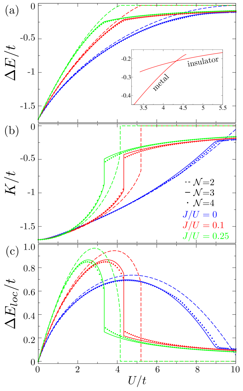
Figure 1: Zero temperature energetics as a function of $U/t$ for various $J/U$ at $\Delta=0$ in the two band Hubbard model for the $d=\infty$ Bethe lattice at half filling. VDAT results for $\mathcal{N}=2,3,4$ are provided. ($a$) The total energy difference $\Delta E(t,U,J)=E(t,U,J)-E(0,U,J)$, where $E(t,U,J)$ is the total energy per site. Inset shows metastable region for $\mathcal{N}=3$ at $J/U=0.1$. ($b$) Kinetic energy per site $K=\langle\hat{K}\rangle/N_{\textrm{site}}$. ($c$) Interaction energy difference $\Delta E_{loc}(t,U,J)=E_{loc}(t,U,J)-E_{loc}(0,U,J)$, where $E_{loc}(t,U,J)$ is the interaction energy per site.

IV.2 Computational complexity of the SCDA

The power of VDAT within the SCDA is that it can be exactly evaluated for $d=\infty$ at a very small computational cost, and here we examine the computational complexity. For simplicity, we focus on the case with translation symmetry, outlined in Section III.2.1. Within a given iteration of the SCDA, there are two relevant scalings to consider: the aspects relevant to $\textrm{\@text@baccent{$\hat{\rho}$}}_{K,k}\left(\lambda,\boldsymbol{S}_{loc}\right)$ and $\textrm{\@text@baccent{$\hat{\rho}$}}_{loc}\left(u,\boldsymbol{\mathcal{G}}\right)$. For the former, the complexity scales linearly in $N_{\textrm{site}}$ and polynomially in $N_{\textrm{orb}}\mathcal{N}$. For the latter, the complexity is independent of $N_{\textrm{site}}$ and scales exponentially in $N_{\textrm{orb}}\mathcal{N}$. Normally, the exponential scaling will be the limiting factor, and therefore we focus on showcasing the cost in specific examples for the two orbital Hubbard model.

For a given $N_{\textrm{orb}}$ and $\mathcal{N}$, there are three relevant tasks for evaluating expectation values under $\textrm{\@text@baccent{$\hat{\rho}$}}_{loc}\left(u,\boldsymbol{\mathcal{G}}\right)$. First, given an input $u$ and $\boldsymbol{\mathcal{G}}$, the $\boldsymbol{g}_{loc}$ and $E_{loc}$ must be computed. Second, the $\boldsymbol{v}_{K}$ and $\boldsymbol{v}_{loc}$ require the computation of the first derivatives $\partial\boldsymbol{g}_{loc}/\partial\boldsymbol{\mathcal{G}}$ and $\partial E_{loc}/\partial\boldsymbol{\mathcal{G}}$ . Third, Eq. 40 must be minimized with respect to $u$, requiring the computation of the polynomial coefficients of $\boldsymbol{g}_{loc}$ and $E_{loc}$ in $u$ given in Eq. 25. For each task, the compiled machine code size and the execution time is provided for $\mathcal{N}=2,3,4$ in Table 1. The machine code size is proportional to the number of instructions which need to be executed. We provide the execution time for $N_{\textrm{orb}}=2$ using a single processor core, demonstrating that the compute time is approximately proportional to the machine code size. The tiny computational times on this modest computational resource illustrates the power of VDAT for the two-orbital Hubbard model. Indeed, all VDAT results generated in this study were executed using a single processing core. It should be noted that $\mathcal{N}=2$ and $\mathcal{N}=3$ are on the same scale, which is true for all $\mathcal{N}=2M$ and $\mathcal{N}=2M+1$ for $M>0$, and this can be understood from the fact that these two cases share the same number of interacting projectors. Given that the minimization over all variational parameters can be achieved on the order of 10 iterations, the total computation time for $\mathcal{N}=4$ is roughly estimated by the cost of task 2 times 10, yielding $\approx 5$ seconds. The total computation time for $\mathcal{N}\leq 3$ is less than one second, and it is dominated by aspects relevant to $\textrm{\@text@baccent{$\hat{\rho}$}}_{K,k}\left(\lambda,\boldsymbol{S}_{loc}\right)$.

	Task1		Task 2		Task 3
$\mathcal{N}$	time (s)	size (Mb)	time (s)	size (Mb)	time (s)	size (Mb)
2	$2\cdot 10^{-5}$	$1.3\cdot 10^{-1}$	$6\cdot 10^{-5}$	$5.1\cdot 10^{-1}$	$4\cdot 10^{-5}$	$2.7\cdot 10^{-1}$
3	$7\cdot 10^{-5}$	$5.2\cdot 10^{-1}$	$3\cdot 10^{-4}$	$3.3$	$2\cdot 10^{-4}$	$1.9$
4	$4\cdot 10^{-2}$	$2.6\cdot 10^{2}$	$5\cdot 10^{-1}$	$3.0\cdot 10^{3}$	$8\cdot 10^{-2}$	$7.2\cdot 10^{2}$

Table 1: Computational cost for various tasks within the SCDA for the two orbital Hubbard model at different $\mathcal{N}$. Each of the three tasks is defined in the main text. The compiled machine code size of the corresponding function and the execution time on a single processor core is provided.

To better understand the scaling for aspects relevant to $\textrm{\@text@baccent{$\hat{\rho}$}}_{loc}\left(u,\boldsymbol{\mathcal{G}}\right)$, it useful to think in terms of the number of effective orbitals $N_{\textrm{eff}}$, which is the number of spin orbitals in the compound space that have a nontrivial interacting projector. For example, for $N_{\textrm{orb}}=2$ at $\mathcal{N}=2-3$ we have $N_{\textrm{eff}}=8$, while for $\mathcal{N}=4-5$ we have $N_{\textrm{eff}}=16$. The computational time $t$ for a given task scales exponentially with $N_{\textrm{eff}}$, so we approximately have $t=c_{0}c_{1}^{N_{\textrm{eff}}}$, and using the results from Table 1 for task 1 with $\mathcal{N}=2$ and $\mathcal{N}=4$, we estimate $c_{0}=10^{-8}$ seconds and $c_{1}=2.6$. Using this simple parametrization, we can estimate the time required for $N_{\textrm{orb}}=5$ and $\mathcal{N}=2-3$, where $N_{\textrm{eff}}=20$, resulting in $t=1.8$ seconds on a single core. In the absence of any symmetry, there will be on the order of $2^{10}$ variational parameters which will need to be minimized. Overall, it appears that generally treating $d$-orbitals with the present algorithm should be tractable for $\mathcal{N}\leq 3$. We can also estimate the time required for $N_{\textrm{orb}}=7$ and $\mathcal{N}=2-3$, where $N_{\textrm{eff}}=28$, resulting in $t=3.6\times 10^{3}$ seconds on a single core. In the absence of symmetry, there will be on the order of $2^{14}$ variational parameters. Therefore, it appears that generally treating $f$-electrons will require parellelization, which can be achieved in a number of ways. Perhaps the simplest approach would be to perform a generalized Hubbard-Stratonovich transformation, recasting the interacting projectors into a sum of non-interacting projectors, and allowing the evaluation of Eq. 25 in a perfectly parallel fashion; dividing the task 1 cost of $t=3.6\times 10^{3}$ by the number of available cores. Therefore, generally treating $f$-electrons for $\mathcal{N}\leq 3$ using reasonable computational resources appears completely tractable.

IV.3 Results

We now illustrate VDAT for the two-orbital Hubbard model in $d=\infty$, where the SCDA exactly evaluates the SPD. Our VDAT results stand alone in the sense that the results monotonically approach the exact solution as $\mathcal{N}$ increases. However, we also compare to published DMFT results using the CTQMC algorithm to solve the DMFT impurity problem, which recovers the numerically exact results at a finite temperature [17]. Given that our VDAT results are at zero temperature, one must compare to the finite temperature DMFT results with caution, as the insulating regime will be rather sensitive to temperature. We will focus on the half filled case of two electrons per site in the paramagnetic state (i.e. $n_{1\sigma}+n_{2\sigma}=1$).

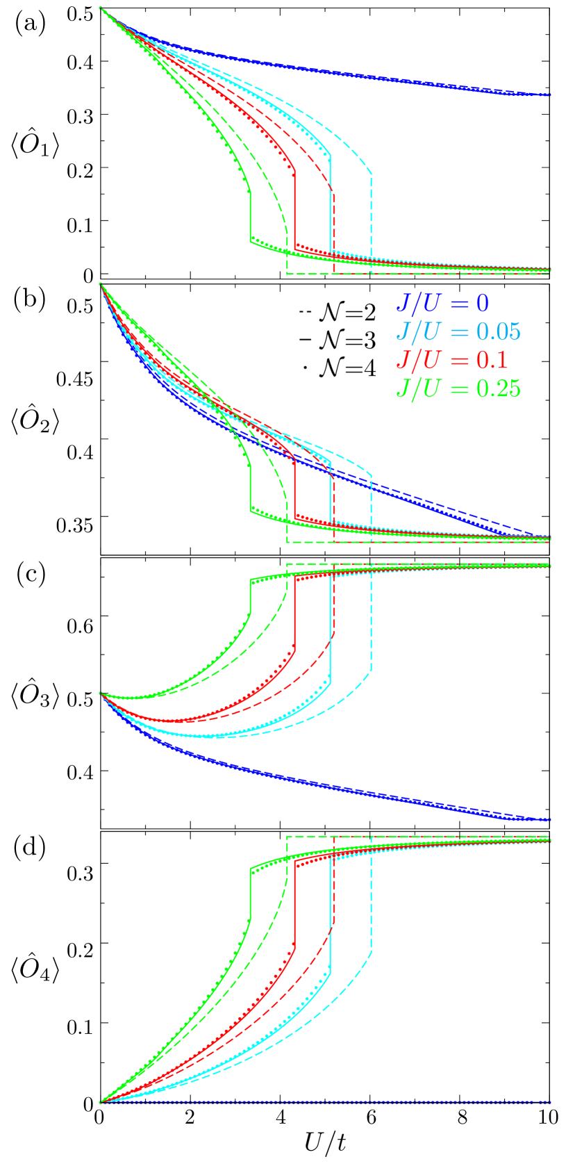
Figure 2: Local two particle correlation functions as a function of $U/t$ for various $J/U$ at $\Delta=0$ in the two band Hubbard model for the $d=\infty$ Bethe lattice at half filling. VDAT results for $\mathcal{N}=2,3,4$ are provided. Panels $a$-$d$ are expectation values of the operators defined in Eqns. 43-45.

We begin by considering the all of the different components of the energy at $\Delta=0$ for a broad range of $J$ and $U$. The total energy is computed using $\mathcal{N}=2,3,4$ with $J/U=0,0.1,0.25$ over a dense grid of $U/t\in[0,10]$ (see Figure 1, panel $a$). In order to facilitate comparison, we plot the difference in the total energy and the atomic energy, where the latter is $E(0,U,J)=U-3J$. For a given $U$ and $J$, the total energy strictly decreases as $\mathcal{N}$ increases, as is required by the variational principle. The $\mathcal{N}=2$ result recovers the usual Gutzwiller approximation, and yields an insulator which is simply a collection of atoms. Clearly, $\mathcal{N}=3$ produces a substantial quantitative improvement over $\mathcal{N}=2$, in addition to a realistic insulating state which allows for virtual hopping. The $\mathcal{N}=4$ result only produces a small quantitative change as compared to $\mathcal{N}=3$, demonstrating that both $\mathcal{N}=3$ and $\mathcal{N}=4$ are close to the exact solution. We now focus on the qualitative nature of the MIT. For $J/U>0$, a clear kink in the total energy as a function of $U/t$ can be observed for all $\mathcal{N}$, indicating a first-order MIT. For $\mathcal{N}=3$, we illustrate the metastable regime by initiating calculations from both metallic and insulating solutions (see Figure 1, panel $a$ inset). Alternatively, for $J/U=0$, the MIT is continuous for all $\mathcal{N}$. For $\mathcal{N}=2$, our results are consistent with previous findings using the Gutzwiller approximation [53]. For $\mathcal{N}\geq 3$ and $J/U>0$, the fact that the first order transition survives is consistent with DMFT calculations which used DMRG [54] or NRG[31] solvers.

It is also interesting to separately consider the kinetic and interaction energy (see Figure 1, panel $b$ and $c$, respectively), which probe the derivative of the total energy with respect to $t$ and $U$ (assuming fixed $J/U$), respectively. The kinetic energy increases with increasing $\mathcal{N}$ in the metallic regime and decreases in the insulating regime. The opposite behavior is observed for the interaction energy. Additionally, a clear discontinuity can be observed at the MIT for $J/U>0$, as the MIT is first-order, whereas a kink is observed for $J/U=0$ as the MIT is continuous.

In order to understand the competition between $U$ and $J$, it is useful to study the individual components of the interaction energy, defined in Eqns. 43-45, and we plot each as a function of $U/t$ for various $J/U$ (see Figure 2). The $\langle\hat{O}_{1}\rangle$, $\langle\hat{O}_{2}\rangle$, and $\langle\hat{O}_{4}\rangle$ all change monotonically as a function of $U$, dictated by the sign of the respective coupling coefficients in the local Hamiltonian, while $\langle\hat{O}_{3}\rangle$ is nonmonotonic in $U$ for finite $J/U$. In the small $U$ regime, the $\langle\hat{O}_{3}\rangle$ decreases, commensurate with the respective coupling coefficient, while in the large $U$ regime it increases due to the prominence of the triplet states.

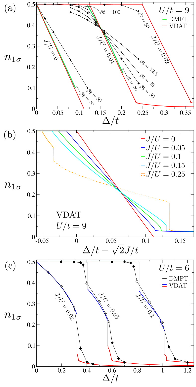
Figure 3: The occupancy $n_{1\sigma}$ as a function of $\Delta$ for various $J/U$ at a given $U/t$ in the two band Hubbard model for the $d=\infty$ Bethe lattice at half filling. VDAT results are presented for $\mathcal{N}=3$, in addition to published DMFT (CTQMC) results[17] at various temperatures. ($a$) Results for $U/t=9$; all VDAT and DMFT results are insulators; thick green lines are extrapolations of the DMFT results to zero temperature (see text for details). ($b$) VDAT results for $U/t=9$ at larger values of $J/U$, where the $x$-axis is shifted by $\sqrt{2}J/t$. Solid lines are insulators, while the dashed line is a metal. ($c$) Results for $U/t=6$. Solid (hollow) DMFT points are insulating (metallic), and red (blue) VDAT lines are insulating (metallic).

We now proceed to more thoroughly explore nonzero $\Delta$, and we begin by examining $n_{1\sigma}$ as a function of $\Delta/t$ at relatively large values of $U/t=6,9$ for various $J/U$ (see Figure 3), which can be compared to previous DMFT calculations [17]. We begin by making general observations about the large $U/t$ insulating regime, where the case of $J=0$ and $J>0$ are qualitatively different (see Figure 3, panel $a$). For $J/U=0$, the system has an approximately constant orbital susceptibility for $\Delta<\Delta_{c}$ and is fully polarized for $\Delta>\Delta_{c}$, where $\Delta_{c}\approx t^{2}/U$. We refer to these two regions as partially and fully orbitally polarized insulators, respectively. For $J/U>0$, the orbital susceptibility is zero for $\Delta<\Delta_{c_{1}}$, approximately constant for $\Delta_{c_{1}}<\Delta<\Delta_{c_{2}}$, and determined from $n_{1\sigma}\approx J^{2}/(16\Delta^{2})$ for $\Delta>\Delta_{c_{2}}$; where $\Delta_{c_{1}}\approx\sqrt{2}J$ and $\Delta_{c_{2}}\approx\Delta_{c_{1}}+t^{2}/U$. We refer to these three regions as zero, partially, and largely orbitally polarized Mott insulators. The underlying physics of these different regions has been discussed previously [17], but the nature of the transition between these regions at zero temperature has not been resolved.

At $U/t=9$, the system is insulating for all values of $\Delta/t$ and $J/U$ (see Figure 3, panel $a$). Interestingly, the polarization (i.e. $n_{2\sigma}-n_{1\sigma}$) at the transition point between the partially and largely orbitally polarized insulators is roughly independent of $J$ and $U$, and occurs at $n_{1\sigma}\approx n_{1\sigma}^{\star}=1/2-\sqrt{2}/3\approx 0.0286$. In contrast to $J=0$, for finite $J$ the system will not fully polarize for finite $\Delta$. The previously published DMFT results are strongly affected by temperature, as illustrated by the calculations for $J/U=0.01$ at $\beta t=12.5,25,50,100$. We extrapolate the DMFT results to $\beta t\rightarrow\infty$, which agrees well with our zero temperature $\mathcal{N}=3$ results for the zero and partially orbitally polarized insulators, while the DMFT results were not computed for the largely orbitally polarized insulator. For $J/U=0$, only $\beta t=50$ was computed with DMFT, and we approximately extrapolate their results to zero temperature by approximating the entropy. The crystal field for a given $n_{1\sigma}$ can be computed from the free energy as $\Delta_{T}=-\left(1/4\right)\partial F(T,n_{1\sigma})/\partial n_{1\sigma}$, where $F(T,n_{1\sigma})=E(T,n_{1\sigma})-TS(T,n_{1\sigma})$ and $E(T,n_{1\sigma})$ is the Legendre transform of the total energy with respect to $\Delta$ where the polarization is parametrized in terms of $n_{1\sigma}$. We assume that $E(0,n_{1\sigma})\approx E(T,n_{1\sigma})$ for small $T$, so the zero temperature crystal field can be approximated as $\Delta_{T=0}=-\left(1/4\right)\partial E(T,n_{1\sigma})/\partial n_{1\sigma}$. To estimate $S(T,n_{1\sigma})$, we use the atomic limit to approximate $S(T,1/2)\approx\ln 6$ and $S(T,0)=0$. Given the symmetry between $n_{1\sigma}$ and $n_{2\sigma}$, we assume that $S(T,n_{1\sigma})$ is quadratic about $n_{1\sigma}=1/2$, and thus we approximate $S(T,n_{1\sigma})\approx(1-4(n_{1\sigma}-\frac{1}{2})^{2})\ln 6$, yielding $\Delta_{T=0}-\Delta_{T}\approx 2\ln 6\left(n_{1\sigma}-\frac{1}{2}\right)T.$ The green curve removes this finite temperature contribution from the DMFT result, yielding excellent agreement with our $\mathcal{N}=3$ result. For $J=0$, the temperature effect is straightforward: for $n_{1\sigma}<1/2$, we have $\Delta_{T=0}<\Delta_{T}$ due to the fact that finite temperature favors the high entropy state with zero polarization. However, for $J>0$, the effect of temperature is clearly more subtle. We see temperature plays opposite roles in the small and large orbital polarization regime. It is also interesting to explore larger values of $J/U$ (see Figure 3, panel $b$), and for a convenient comparison, we shift the $x$-axis by $\sqrt{2}J/t$. As $J/U$ increases, the orbital susceptibility decreases, and the transition from the partially to largely orbitally polarized Mott insulator is first order for $J/U=0.1,0.15$. For $J/U=0.25$ the crystal field drives a first-order MIT from a partially orbitally polarized Mott insulator to a metal followed by another first-order MIT to a largely orbitally polarized Mott insulator. At $U/t=6$ (see Figure 3, panel $c$), the results contain both metallic and insulating phases, and VDAT can faithfully capture the details of the metal-insulator transition. The differences between VDAT and DMFT are relatively small in this case, and are likely attributable to the finite temperature of the DMFT calculations.

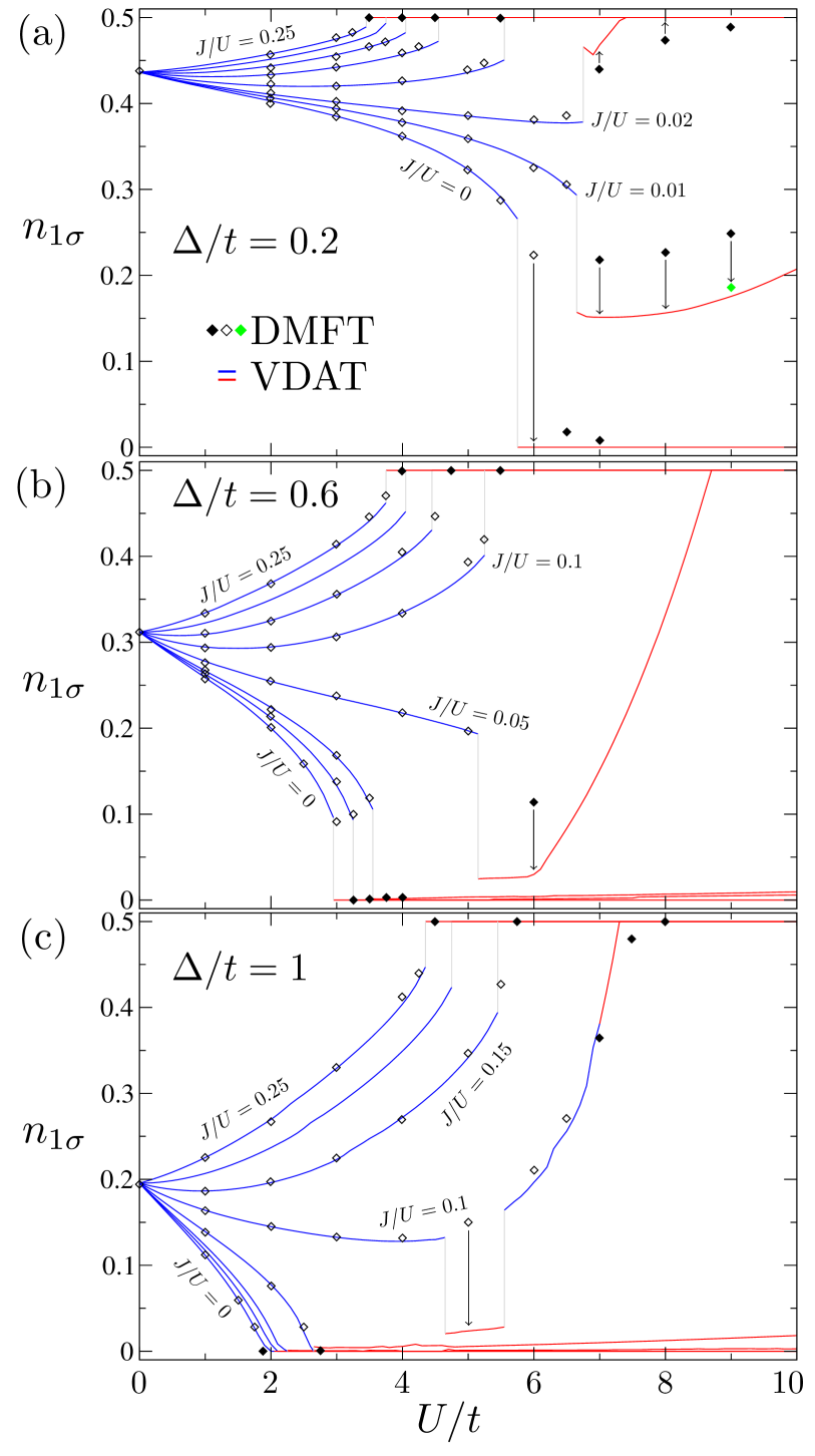
Figure 4: The occupancy $n_{1\sigma}$ as a function of $U/t$ for various $J/U$ at a given $\Delta/t$ in the two band Hubbard model for the $d=\infty$ Bethe lattice at half filling. VDAT results are presented for $\mathcal{N}=3$, in addition to published DMFT (CTQMC) results at $\beta t=50$[17]. VDAT results for $J/U=0,0.01,0.02,0.05,0.1,0.15,0.2,0.25$ are provided in each panel (select curves are labeled), and corresponding DMFT results are provided where available (arrows are used when the correspondence is unclear). Red (blue) VDAT lines are insulating (metallic), while black solid (hollow) DMFT points are insulating (metallic); and the green DMFT point is an extrapolation to zero temperature (see text for details). ($a$) $\Delta/t=0.2$ ($b$) $\Delta/t=0.6$ ($c$) $\Delta/t=1$.

The previous results focused more on the large $U/t$ regime, and here we explore a broad range of $U/t$ for various values of $J/U$ and $\Delta/t$ (see Figure 4). Overall, there is excellent agreement with DMFT in the metallic region, while there are nontrivial differences in the insulating regime which are likely due to the finite temperature of the DMFT calculations. The zero temperature extrapolation of the DMFT results for $U/t=9$ and $J/U=0.01$ and $\Delta/t=0.2$ from Figure 3$a$ is plotted as a green point in Figure 4$a$, showing good agreement with our VDAT results. Interestingly, at $\Delta/t=0.6$ and $J/U=0.05$ (see Figure 4, panel $b$), increasing $U/t$ drives a transition from a metal to a largely orbitally polarized Mott insulator which then transitions to a partially orbitally polarized Mott insulator followed by a zero orbitally polarized Mott insulator. Similar behavior is observed for $\Delta/t=1.0$ and $J/U=0.1$ (see Figure 4, panel $c$), though the system becomes has an additional first order transition from the largely orbitally polarized Mott insulator to a metal before transitioning to the partially orbitally polarized Mott insulator.

In order to obtain a detailed understanding over the entire phase space of parameters, we evaluate the quasiparticle weight as function of $U/t$ and $n_{1\sigma}$ for various $J/U$, which serves as a phase diagram of the metal-insulator transition (see Figure 5). Additionally, a Maxwell construction is used to determine if a given value of $n_{1\sigma}$ is stable with respect to $\Delta$, and hatched lines are used to denote unstable regions. We used two resolutions for the phase diagram: 0.1 in $U/t$ and 0.01 in $n_{1\sigma}$ for $n_{1\sigma}>0.05$, and 0.01 in $U/t$ and 0.001 in $n_{1\sigma}$ for $n_{1\sigma}<0.05$, yielding a total of 55,000 calculations per phase diagram, and this level of resolution would be formidable using DMFT. In the region of large polarization (i.e. $n_{1\sigma}\rightarrow 0$), the kinetic energy is approaching zero, making the convergence of the calculation challenging; this region would be best explored by treating $n_{1\sigma}$ as a perturbation parameter, but we leave this for future work. For $J/U=0$ (see Figure 5, panel $a$), at $n_{1\sigma}=1/2$ there is a MIT at $U/t=9.1$, and the transition value of $U/t$ decreases monotonically for decreasing $n_{1\sigma}$. In the large polarization limit where $n_{1\sigma}\rightarrow 0$, there is a band-insulator to fully polarized Mott insulator transition at finite $U/t$. Furthermore, for $2.3\leq U/t\leq 8$ there is a first-order MIT driven by $\Delta$ (denoted by hatching), and three regimes can be seen. For the smallest $U/t$ region, there is a metal to band insulator transition; for intermediate $U/t$, there is a metal to fully orbitally polarized Mott insulator transition; for largest $U/t$, there is a metal to partially orbitally polarized Mott insulator transition.

For $J/U>0$ (see Figure 5, panels $b$-$f$), the metal to insulator transition value of $U/t$ is no longer a monotonic function of $n_{1\sigma}$. There is a first-order insulator to metal transition in $\Delta$ around $n_{1\sigma}=1/2$, and the range increases with $J/U$. For sufficiently large $J/U$ in the large polarization region, the zero quasiparticle weight boundary coincides with the first-order phase boundary. Additionally, there is an approximately vertical boundary between the partially and largely orbitally polarized Mott insulators, which becomes first-order for sufficiently large $J/U$. Finally, the quasiparticle weight decreases as $n_{1\sigma}\rightarrow 0$ for all $U/t>0$, and this is most easily seen for the larger values of $J/U$. This behavior is expected given our scaling analysis in Section IV.1, which suggests that for $n_{1\sigma}<\alpha J^{2}$ the quasiparticle weight is zero, where $\alpha$ is a positive constant. Given the numerical difficulty for treating small values of $n_{1\sigma}$ (i.e. $n_{1\sigma}<0.01$), it would be preferable to explore this regime treating $n_{1\sigma}$ as a small parameter, which would allow for an analytic evaluation using $\mathcal{N}=3$. Such an exercise would clearly answer whether or not the Mott insulator exists for infinitesimal $U/t$ with fixed $J/U>0$ in the large polarization limit. Nonetheless, the presence of strong electronic correlations in the largely polarized regime is clear. Therefore, crystals bearing $d$-electrons or $f$-electrons which are nominally a band insulator, according to experiment or density functional theory, may in reality be in this largely polarized regime which has nontrivial electronic correlations. In future work, we will investigate the doping dependence of this regime.

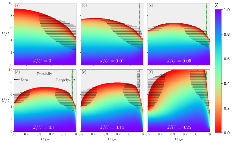
Figure 5: VDAT $\mathcal{N}=3$ results for the quasiparticle weight $Z$ as a function of $n_{1\sigma}$ and $U/t$ for various $J/U$ in the two band Hubbard model for the $d=\infty$ Bethe lattice at half filling. The quasiparticle weight is zero when the color is grey. The black hatched lines indicate unstable regions. The vertical green lines at $n_{1\sigma}=1/2-\sqrt{2}/3\approx 0.0286$ indicate the boundary between the partially and largely orbitally polarized Mott insulator for $U/t\rightarrow\infty$. For $J/U=0.1$, the zero, partially, and largely orbitally polarized Mott insulating regimes are labeled.

V Conclusions and Future Outlook

In this work, we applied the recently developed VDAT within the SCDA to the two-orbital Hubbard model in $d=\infty$. The SCDA is a self-consistent algorithm to compute the total energy under the SPD using an iterative approach, and this poses a serious technical challenge of how to efficiently compute the derivatives of the total energy with respect to the variational parameters. We surmounted this challenge using an iterative decoupled minimization algorithm. At each iteration, the variational parameters are updated using a local effective model and a collection of independent effective models for the $k$-points, and the SCDA self-consistency is maintained using a fixed point method. In addition to this minimization algorithm, two formal developments were made to VDAT. First, we provided a diagrammatic proof of the equivalence of integer time correlation functions under the SPD to corresponding observables measured in the compound space. Second, we identified the gauge symmetry of the SPD, and we proposed various schemes for fixing the gauge freedom, which is of practical importance for stabilizing the minimization within the SCDA.

Using the aforementioned formal and technical developments, we studied the half filled two orbital Hubbard model in $d=\infty$ over a broad range of parameter space in $U/t$, $J/U$, and $\Delta/t$ at zero temperature. The computational cost of VDAT for this model is negligible, requiring approximately one second on a single processor core at $\mathcal{N}=3$ to solve the model for a given $U/t$, $J/U$, and $\Delta/t$. At $\Delta=0$, we evaluated $\mathcal{N}=2,3,4$, where $\mathcal{N}=2$ recovers the Gutzwiller approximation, and the results for $\mathcal{N}=3,4$ only exhibited very small differences, suggesting the results are largely converged with respect to $\mathcal{N}$. Given that increasing $\mathcal{N}$ monotonically approaches the exact solution, $\mathcal{N}=3,4$ should be close to the exact solution, and therefore $\mathcal{N}=3$ should serve as a standard theory of Mott and Hund physics in the $d=\infty$ Hubbard model. VDAT for $\mathcal{N}>2$ confirms the previous Gutzwiller results (i.e. $\mathcal{N}=2)$ that the $U$ driven MIT for $\Delta=0$ (i.e. $n_{1\sigma}=1/2$) and $J>0$ is first-order, and is continuous for $J=0$. For $\Delta>0$ and $J>0$, VDAT for $\mathcal{N}=3$ confirms previous finite temperature DMFT results of a zero orbital susceptibility region for $\Delta\apprle\sqrt{2}J$, and confirms previous conjectures that the transition to finite susceptibility is sharp at zero temperature[17]. At intermediate values of $U/t$ and sufficiently large values of $J/U$, there exists a first-order $\Delta$ driven MIT going from a zero orbitally polarized Mott insulator to a partially polarized metal, followed by a first-order transition to either a partially or largely orbitally polarized Mott insulator. For large $U/t$, there is a $\Delta$ driven transition from a partially to a largely orbitally polarized Mott insulator, and this transition appears to be continuous at small $J/U$ and first-order at large $J/U$. Finally, for nonzero $J/U$, the quasiparticle weight decreases as $n_{1\sigma}\rightarrow 0$ for all nonzero $U/t$, and this VDAT result is consistent with scaling arguments in the large polarization limit. Detailed phase diagrams of the quasiparticle weight as a function of $n_{1\sigma}$ and $U/t$ are presented at an unprecedented resolution. In summary, VDAT uncovered qualitative physics which had not yet been resolved, and this is due to the fact that VDAT operates at zero temperature and exactly evaluates the SPD ansatz for arbitrary $U$, $J$, and $\Delta$.

Analogous to DMFT, VDAT within the SCDA can be straightforwardly applied in finite dimensions as a local approximation. Therefore, VDAT within the SCDA at $\mathcal{N}=3$ will likely become a de facto standard for probing the local physics of multiband Hubbard models at zero temperature, delivering the quality of DMFT at a cost not far beyond the Gutzwiller approximation. An obvious next step will be to combine VDAT within the SCDA with DFT, in the same spirit of DFT plus Gutzwiller[55]. DFT+VDAT($\mathcal{N}=3$) will have similar quality to DFT+DMFT at a cost similar to DFT+Gutzwiller, and DFT+VDAT will have distinct advantages over DFT+DMFT in that it naturally accesses zero temperature.

Another important future direction will be executing VDAT within finite dimensions. There are various approaches to extend DMFT to finite dimensions, such as cluster DMFT[49, 2], dual Fermions[50], the dynamical vertex approximation[50], etc, and it is clear that integer time analogues can be pursued within VDAT. Given the massive speedup of VDAT within the SCDA relative to DMFT, it seems likely that there will be a similar speedup when applying VDAT to finite dimensions. Therefore, it seems possible that the SPD at $\mathcal{N}=3$ and beyond can be precisely evaluated using VDAT in finite dimensions, allowing for a zero temperature solution that would compete with all existing state-of-the-art methods for the single band Hubbard model[6].

VI Acknowledgments

This work was supported by the Columbia Center for Computational Electrochemistry.

VII Appendix

Here we review some key properties of non-interacting many-body density matrices and derive an explicit expression for $̱\hat{Q}$. Consider a generalized non-interacting many-body density matrix $\hat{\rho}_{0}=\exp\left(\boldsymbol{v}\cdot\hat{\boldsymbol{n}}\right)$, where $\hat{\rho}_{0}$ is generalized in the sense that $\boldsymbol{v}$ is an arbitrary matrix. The following set of identities are useful when evaluating the non-interacting integer time Green’s function

$$\hat{\rho}_{0}^{-1}\hat{a}_{i}^{\dagger}\hat{\rho}_{0}=\sum_{i^{\prime}}\left[\bm{S}_{0}\right]_{ii^{\prime}}\hat{a}_{i^{\prime}}^{\dagger},$$ (49)

$$\hat{\rho}_{0}\hat{a}_{i}^{\dagger}\hat{\rho}_{0}^{-1}=\sum_{i^{\prime}}\left[\bm{S}_{0}^{-1}\right]_{ii^{\prime}}\hat{a}_{i^{\prime}}^{\dagger},$$ (50)

$$\hat{\rho}_{0}^{-1}\hat{a}_{i}\hat{\rho}_{0}=\sum_{i^{\prime}}\hat{a}_{i^{\prime}}\left[\bm{S}_{0}^{-1}\right]_{i^{\prime}i},$$ (51)

$$\hat{\rho}_{0}\hat{a}_{i}\hat{\rho}_{0}^{-1}=\sum_{i^{\prime}}\hat{a}_{i^{\prime}}\left[\bm{S}_{0}\right]_{i^{\prime}i},$$ (52)

where $\boldsymbol{S}_{0}=\exp\left(-\boldsymbol{v}^{T}\right)$. In order to prove Eq. 49, we first prove that it holds for an infinitesimal $\tilde{\boldsymbol{v}}$ by directly evaluating

$$\exp\left(-\tilde{\boldsymbol{v}}\cdot\hat{\boldsymbol{n}}\right)\hat{a}_{i}^{\dagger}\exp\left(\tilde{\boldsymbol{v}}\cdot\hat{\boldsymbol{n}}\right)=\hat{a}_{i}^{\dagger}+\left[\hat{a}_{i}^{\dagger},\tilde{\boldsymbol{v}}\cdot\hat{\boldsymbol{n}}\right]$$

$$=\hat{a}_{i}^{\dagger}-\sum_{i^{\prime}}[\tilde{\boldsymbol{v}}]_{i^{\prime}i}\hat{a}_{i^{\prime}}^{\dagger}=\sum_{i^{\prime}}[\tilde{\boldsymbol{S}}_{0}]_{ii^{\prime}}\hat{a}_{i^{\prime}}^{\dagger},$$ (53)

where $\tilde{\boldsymbol{S}}_{0}=\exp\left(-\tilde{\boldsymbol{v}}^{T}\right)$. For a finite $\boldsymbol{v}$, consider $\tilde{\boldsymbol{v}}=\boldsymbol{v}/N$ and iteratively apply Eq. 53 $N$ times with $N\rightarrow\infty$, which proves Eq. 49. Equations 50-52 can then be derived from Eq. 49. Using the preceding identities, we can derive

$$\frac{\textrm{Tr}(\hat{\rho}_{0}\hat{a}_{i}^{\dagger}\hat{a}_{j})}{\textrm{Tr}(\hat{\rho}_{0})}=\left[\frac{\boldsymbol{1}}{\boldsymbol{1}+\boldsymbol{S}_{0}}\right]_{ij}.$$ (54)

We now proceed to derive an explicit expression for $̱\hat{Q}$, and to simplify notation we consider $L=1$, though the derivation is general. We begin by explicitly evaluating $\boldsymbol{g}_{Q}$ using Eq. 93 in Ref. [43], resulting in

$$[\boldsymbol{g}_{Q}]_{\tau\tau^{\prime}}=\frac{1}{2}\textrm{sign}(\tau^{\prime}-\tau+\frac{1}{2}).$$ (55)

Using Eqns. 112 and 113 from Ref. [43], we obtain

$$\textrm{\@text@baccent{$\hat{Q}$}}=\exp\left(-\ln\left(\bm{S}_{Q}^{T}\right)\cdot\textrm{\@text@baccent{$\hat{\boldsymbol{n}}$}}\right)=\exp\left(\ln\left(\bm{S}_{Q}\right)\cdot\textrm{\@text@baccent{$\hat{\boldsymbol{n}}$}}\right),$$ (56)

where $\boldsymbol{S}_{Q}=\boldsymbol{g}_{Q}^{-1}-\boldsymbol{1}$, and the matrix elements are

$$[\boldsymbol{S}_{Q}]_{\tau\tau^{\prime}}=-\delta_{\tau+1,\tau^{\prime}}+\delta_{\tau-\mathcal{N}+1,\tau^{\prime}},$$ (57)

which implies $\boldsymbol{S}_{Q}^{-1}=\boldsymbol{S}_{Q}^{T}=\boldsymbol{S}_{Q}^{\dagger}$ and $\textrm{\@text@baccent{$\hat{Q}$}}^{\dagger}=\textrm{\@text@baccent{$\hat{Q}$}}^{-1}$. We can now compute

$$\ln\bm{S}_{Q}=\sum_{\omega}\ln\left(-\lambda_{\omega}\right)v_{\omega}v_{\omega}^{T},$$ (58)

where $\omega=\frac{2\pi}{\mathcal{N}}m$ and $m=1,2,\dots,\mathcal{N}$ and $\lambda_{\omega}=\exp\left(i\left(\omega-\frac{\pi}{\mathcal{N}}\right)\right)$ and

$$v_{\omega}=\frac{1}{\sqrt{\mathcal{N}}}\left(1,\lambda_{\omega}^{1},\dots,\lambda_{\omega}^{\mathcal{N}-1}\right)^{T}.$$ (59)

The matrix elements of $\ln\boldsymbol{S}_{Q}$ can then be evaluated as

$$[\ln\bm{S}_{Q}]_{\tau\tau^{\prime}} =\frac{i}{\mathcal{N}}\sum_{\omega}\left(\omega-\frac{\pi}{\mathcal{N}}-\pi\right)\lambda_{\omega}^{\tau-\tau^{\prime}}$$ (60)

$$=\begin{cases}0&\tau=\tau^{\prime}\\ \frac{\pi}{\mathcal{N}}\frac{1}{\sin\left(\pi\left(\tau-\tau^{\prime}\right)/\mathcal{N}\right)}&\tau\neq\tau^{\prime}\end{cases}.$$ (61)

Finally, using Eqns. 49-52 and Eq. 57, we obtain

$$\textrm{\@text@baccent{$\hat{Q}$}}^{-1}\textrm{\@text@baccent{$\hat{a}$}}^{\dagger\left(\tau\right)}\textrm{\@text@baccent{$\hat{Q}$}}=-\textrm{\@text@baccent{$\hat{a}$}}^{\dagger\left(\tau+1\right)},$$ (62)

$$\textrm{\@text@baccent{$\hat{Q}$}}\textrm{\@text@baccent{$\hat{a}$}}^{\dagger\left(\tau\right)}\textrm{\@text@baccent{$\hat{Q}$}}^{-1}=-\textrm{\@text@baccent{$\hat{a}$}}^{\dagger\left(\tau-1\right)},$$ (63)

$$\textrm{\@text@baccent{$\hat{Q}$}}^{-1}\textrm{\@text@baccent{$\hat{a}$}}^{\left(\tau\right)}\textrm{\@text@baccent{$\hat{Q}$}}=-\textrm{\@text@baccent{$\hat{a}$}}^{\left(\tau+1\right)},$$ (64)

$$\textrm{\@text@baccent{$\hat{Q}$}}\textrm{\@text@baccent{$\hat{a}$}}^{\left(\tau\right)}\textrm{\@text@baccent{$\hat{Q}$}}^{-1}=-\textrm{\@text@baccent{$\hat{a}$}}^{\left(\tau-1\right)},$$ (65)

where we define $\textrm{\@text@baccent{$\hat{a}$}}_{\ell}^{\dagger(\mathcal{N}+1)}\equiv-\textrm{\@text@baccent{$\hat{a}$}}_{\ell}^{\dagger(1)}$ and $\textrm{\@text@baccent{$\hat{a}$}}_{\ell}^{\dagger(0)}\equiv-\textrm{\@text@baccent{$\hat{a}$}}_{\ell}^{\dagger(\mathcal{N})}$.

References

• Imada et al. [1998] M. Imada, A. Fujimori, and Y. Tokura, Rev. Mod. Phys. 70, 1039 (1998).
• Kotliar et al. [2006] G. Kotliar, S. Y. Savrasov, K. Haule, V. S. Oudovenko, O. Parcollet, and C. A. Marianetti, Rev. Mod. Phys. 78, 865 (2006).
• Montorsi [1992] A. Montorsi, The Hubbard Model - A Reprint Volume (World Scientific, Singapore, 1992).
• Gebhard [1997] F. Gebhard, The Mott Metal-Insulator Transition - Models And Methods (Springer Science and Business Media, Berlin, 1997).
• Essler et al. [2005] F. H. L. Essler, H. Frahm, F. Gohmann, A. Klumper, and V. E. Korepin, The One-Dimensional Hubbard Model (Cambridge University Press, Cambridge, 2005).
• Leblanc et al. [2015] J. Leblanc, A. E. Antipov, F. Becca, I. W. Bulik, G. Chan, C. M. Chung, Y. J. Deng, M. Ferrero, T. M. Henderson, C. A. Jimenez-hoyos, E. Kozik, X. W. Liu, A. J. Millis, N. V. Prokof’ev, M. P. Qin, G. E. Scuseria, H. Shi, B. V. Svistunov, L. F. Tocchio, I. S. Tupitsyn, S. R. White, S. W. Zhang, B. X. Zheng, Z. Y. Zhu, and E. Gull, Physical Review X 5, 041041 (2015).
• Kaushal et al. [2017] N. Kaushal, J. Herbrych, A. Nocera, G. Alvarez, A. Moreo, F. A. Reboredo, and E. Dagotto, Phys. Rev. B 96, 155111 (2017).
• Tocchio et al. [2016] L. F. Tocchio, F. Arrigoni, S. Sorella, and F. Becca, Journal Of Physics-condensed Matter 28, 105602 (2016).
• franco et al. [2018] C. D. franco, L. F. Tocchio, and F. Becca, Phys. Rev. B 98, 075117 (2018).
• Georges et al. [1996] A. Georges, G. Kotliar, W. Krauth, and M. J. Rozenberg, Rev. Mod. Phys. 68, 13 (1996).
• Kotliar and Vollhardt [2004] G. Kotliar and D. Vollhardt, Physics Today 57, 53 (2004).
• Vollhardt [2012] D. Vollhardt, Annalen Der Physik 524, 1 (2012).
• Gull et al. [2011] E. Gull, A. J. Millis, A. I. Lichtenstein, A. N. Rubtsov, M. Troyer, and P. Werner, Rev. Mod. Phys. 83, 349 (2011).
• Werner et al. [2006] P. Werner, A. Comanac, L. D. Medici, M. Troyer, and A. J. Millis, Phys. Rev. Lett. 97, 076405 (2006).
• Haule [2007] K. Haule, Phys. Rev. B 75, 155113 (2007).
• Werner and Millis [2006] P. Werner and A. J. Millis, Phys. Rev. B 74, 155107 (2006).
• Werner and Millis [2007] P. Werner and A. J. Millis, Phys. Rev. Lett. 99, 126405 (2007).
• Werner et al. [2008] P. Werner, E. Gull, M. Troyer, and A. J. Millis, Phys. Rev. Lett. 101, 166405 (2008).
• Poteryaev et al. [2008] A. I. Poteryaev, M. Ferrero, A. Georges, and O. Parcollet, Phys. Rev. B 78, 045115 (2008).
• Werner et al. [2009] P. Werner, E. Gull, and A. J. Millis, Phys. Rev. B 79, 115119 (2009).
• Kita et al. [2011] T. Kita, T. Ohashi, and N. Kawakami, Phys. Rev. B 84, 195130 (2011).
• Hoshino and Werner [2015] S. Hoshino and P. Werner, Phys. Rev. Lett. 115, 247001 (2015).
• Ryee et al. [2021] S. Ryee, M. J. Han, and S. Choi, Phys. Rev. Lett. 126, 206401 (2021).
• Caffarel and Krauth [1994] M. Caffarel and W. Krauth, Phys. Rev. Lett. 72, 1545 (1994).
• Wilson [1975] K. G. Wilson, Rev. Mod. Phys. 47, 773 (1975).
• Wilson [1983] K. G. Wilson, Rev. Mod. Phys. 55, 583 (1983).
• Bulla et al. [2008] R. Bulla, T. A. Costi, and T. Pruschke, Rev. Mod. Phys. 80, 395 (2008).
• Schollwock [2005] U. Schollwock, Rev. Mod. Phys. 77, 259 (2005).
• Schollwock [2011] U. Schollwock, Annals Of Physics 326, 96 (2011).
• Peters [2011] R. Peters, Phys. Rev. B 84, 075139 (2011).
• Pruschke and Bulla [2005] T. Pruschke and R. Bulla, European Physical Journal B 44, 217 (2005).
• Stadler et al. [2015] K. M. Stadler, Z. P. Yin, J. V. delft, G. Kotliar, and A. Weichselbaum, Phys. Rev. Lett. 115, 136401 (2015).
• Kugler et al. [2019] F. B. Kugler, S. Lee, A. Weichselbaum, G. Kotliar, and J. V. delft, Phys. Rev. B 100, 115159 (2019).
• Kugler et al. [2020] F. B. Kugler, M. Zingl, H. Strand, S. Lee, J. V. delft, and A. Georges, Phys. Rev. Lett. 124, 016401 (2020).
• Kuhner and White [1999] T. D. Kuhner and S. R. White, Phys. Rev. B 60, 335 (1999).
• Jeckelmann [2002] E. Jeckelmann, Phys. Rev. B 66, 045114 (2002).
• White and Feiguin [2004] S. R. White and A. E. Feiguin, Phys. Rev. Lett. 93, 076401 (2004).
• Daley et al. [2004] A. J. Daley, C. Kollath, U. Schollwock, and G. Vidal, Journal Of Statistical Mechanics-theory And Experiment , P04005 (2004).
• Fernandez and Hallberg [2018] Y. N. Fernandez and K. Hallberg, Frontiers In Physics 6, 13 (2018).
• Nunez-fernandez et al. [2018] Y. Nunez-fernandez, G. Kotliar, and K. Hallberg, Phys. Rev. B 97, 121113 (2018).
• Hallberg and Nunez-fernandez [2020] K. Hallberg and Y. Nunez-fernandez, Physical Review B 102, 245138 (2020).
• Boidi et al. [2021] N. A. Boidi, H. F. Garcia, Y. Nunez-fernandez, and K. Hallberg, Physical Review Research 3, 043213 (2021).
• Cheng and Marianetti [2021a] Z. Q. Cheng and C. A. Marianetti, Phys. Rev. B 103, 195138 (2021a).
• Cheng and Marianetti [2021b] Z. Q. Cheng and C. A. Marianetti, Phys. Rev. Lett. 126, 206402 (2021b).
• Metzner and Vollhardt [1987] W. Metzner and D. Vollhardt, Phys. Rev. Lett. 59, 121 (1987).
• Metzner and Vollhardt [1988] W. Metzner and D. Vollhardt, Phys. Rev. B 37, 7382 (1988).
• Metzner and Vollhardt [1989] W. Metzner and D. Vollhardt, Phys. Rev. Lett. 62, 324 (1989).
• Bunemann et al. [1997] J. Bunemann, F. Gebhard, and W. Weber, Journal Of Physics-condensed Matter 9, 7343 (1997).
• Maier et al. [2005] T. Maier, M. Jarrell, T. Pruschke, and M. H. Hettler, Rev. Mod. Phys. 77, 1027 (2005).
• Rohringer et al. [2018] G. Rohringer, H. Hafermann, A. Toschi, A. A. Katanin, A. E. Antipov, M. I. Katsnelson, A. I. Lichtenstein, A. N. Rubtsov, and K. Held, Rev. Mod. Phys. 90, 025003 (2018).
• Rubtsov et al. [2008] A. N. Rubtsov, M. I. Katsnelson, and A. I. Lichtenstein, Phys. Rev. B 77, 033101 (2008).
• [52] See Supplemental Material at [URL will be inserted by publisher] for the eigenstates of the local Hamiltonian for the two-orbital Hubbard model and the gauge freedom at $\mathcal{N}=4$.
• Bunemann et al. [1998] J. Bunemann, W. Weber, and F. Gebhard, Phys. Rev. B 57, 6896 (1998).
• Hallberg et al. [2015] K. Hallberg, D. J. Garcia, P. S. Cornaglia, J. I. Facio, and Y. Nunez-fernandez, Epl 112, 17001 (2015).
• Deng et al. [2009] X. Y. Deng, L. Wang, X. Dai, and Z. Fang, Phys. Rev. B 79, 075114 (2009).