Suzaku Observations of the Cluster Outskirts and Intercluster Filament in the Triple Merger Cluster Abell 98

Abstract

We present Suzaku observations of the Abell 98 (A98) triple galaxy cluster system and the purported intercluster filament. The three subclusters are expected to lie along a large scale cosmic filament. With partial azimuthal coverage of the northernmost cluster, we find that the inferred entropy profile of this relatively low mass cluster ($kT\approx 2.8$ keV) adheres to expectations from models of self-similar pure gravitational collapse in the region of the virial radius. There is evidence of extended structure beyond $r_{\_}{200}$ to the north of the northernmost cluster, along the merger axis, with properties consistent with what is expected for the warm-hot intergalacitc medium (WHIM; $kT=0.11_{\_}{-0.02}^{+0.01}$ keV, $n_{\_}e={7.6\times 10^{-5}}^{+3.6\times 10^{-5}}_{\_}{-3.6\times 10^{-5}}$ cm^-3). No such emission is detected at the same radius in regions away from the merger axis, consistent with the expectation that the merger axis of this triple system lies along a large scale cosmic filament. In the bridge region between A98N and A98S, there is evidence of filamentary emission at the $2.2\sigma$ level, as well as a tentative detection of cool gas ($kT\sim 1$ keV). The entropy profile of this intercluster filament suggests that the A98 system is most likely aligned closer to the plane of the sky rather than along the line of sight. The structure to the north of the system, as well as in between A98N and A98S is indicative that the clusters are connected to a larger-scale structure spanning at least 4 Mpc.

1 Introduction

Cosmological simulations predict that massive galaxy clusters are generally located at the nodes of the web-like, large-scale structure of the universe (e.g. IllustrisTNG simulation; Nelson et al. (2021)). The assembly and evolution of galaxy clusters throughout time are powerful tools for precision cosmology (e.g. Schellenberger & Reiprich (2017)), which informs our understanding of the growth and evolution of structure. Simulations predict that the baryons in the cosmic web have been shock heated and compressed to electron temperatures $T_{\_}e$ $\approx 10^{5}-10^{7}$ K with electron densities $n_{\_}{e}\approx 10^{-7}-10^{-5}$ cm^-3. This diffuse, primordial baryonic gas is known as the warm-hot intergalactic medium (WHIM), which is thought to comprise of baryons in the local universe (e.g., Bregman, 2007).

One key assumption when using galaxy clusters for precision cosmology is that clusters are in hydrostatic equilibrium. However, it has been observed that many massive galaxy clusters seemingly deviate from hydrostatic equilibrium at large cluster radii (e.g. Walker et al. (2013)). This could be due to a number of physical processes in the intracluster medium (ICM), including clumping of cool gas (Eckert et al., 2015; Simionescu et al., 2011; Tchernin et al., 2016) at large cluster radii ($\sim r_{\_}{200}$ ) biasing the average surface brightness of cluster outskirts high, non-thermal pressure support from bulk motions, turbulence or cosmic rays (Lau et al., 2009; Vazza et al., 2009; Battaglia et al., 2013), and -ion non-equilibrium (Fox & Loeb, 1997; Wong & Sarazin, 2009; Hoshino et al., 2010; Avestruz et al., 2015) (for a review of cluster outskirts, see e.g. Walker et al. (2019)).

The ICM thermodynamic history of clusters is encoded in the entropy profiles of the ICM. Unlike larger mass clusters, studies of lower mass galaxy clusters and groups with Suzaku have shown close agreement in the virialization region between the predicted entropy profiles based on self-similar gravitational collapse models, and the inferred entropy profiles of the systems based on X-ray spectroscopy studies (Su et al., 2015; Bulbul et al., 2016; Sarkar et al., 2021). This could be due to the fact that galaxy groups are likely more evolved than galaxy clusters (Paul et al., 2017).

Another theory is that due to their smaller mass, galaxy groups are more sensitive to common thermodynamic processes such as stellar and active galactic nuclei (AGN) feedback (e.g. Pratt et al., 2010; Lovisari et al., 2015), injecting entropy into their outskirts. This injected entropy could artificially correct for the entropy deficiency observed in more massive clusters around the virialization region, making the ICM of the lower mass cluster or group look like it’s obeying self-similarity. However, an entropy excess at large group and low mass cluster radii has not yet been observed. Isolated groups also tend to be in less dynamically active regions than clusters, as they are not at the nodes of the cosmic web. The relative isolation would lead there to be fewer clumps, weaker accretion shocks, and less turbulence.

Simulations (e.g. Angelinelli et al., 2021) and deep X-ray observations (e.g. Mirakhor & Walker, 2020) of galaxy clusters have revealed that the thermodynamic structure of the outskirts varies azimuthally, presumably due in large part to the growth of hierarchical structure through cosmic filaments. Understanding the physical processes at work in the ICM in the outskirts of clusters is key to our of the growth of cosmic structure, and to using clusters for precision cosmology.

Table 1: J2000 right ascension and declination, redshift ($z$), electron temperature ($T_{\_}e$), and $r_{\_}{500}$ for the three main subclusters consisting of the A98 system.

Object	R.A.	Dec	z	$T_{\_}e$ [keV]	$r_{\_}{500}$ [Mpc]
A98N	$00^{\rm{h}}46^{\rm{m}}25^{\rm{s}}$	$20^{\rm{d}}37^{\rm{m}}14^{\rm{s}}$	0.1043	2.78	0.72
A98S	$00^{\rm{h}}46^{\rm{m}}29^{\rm{s}}$	$20^{\rm{d}}28^{\rm{m}}04^{\rm{s}}$	0.1063	2.82	0.72
A98SS	$00^{\rm{h}}46^{\rm{m}}36^{\rm{s}}$	$20^{\rm{d}}15^{\rm{m}}44^{\rm{s}}$	0.1218	2.42	0.67

Abell 98 consists of three subclusters (Abell et al., 1989); Abell 98N (A98N), Abell 98S (A98S), and Abell 98SS (A98SS). The right ascension and declination (Jones & Forman, 1999; Burns et al., 1994), redshift (White et al., 1997; Pinkney et al., 2000), and measured electron temperature and inferred $r_{\_}{500}$ (Vikhlinin et al., 2009) are presented in Table 1.

The bimodal distribution of A98N and A98S was first seen in the X-ray with the Einstein telescope (Forman et al., 1981; Henry et al., 1981). A98SS was also later observed with the Einstein telescope (Jones & Forman, 1999). The presence of three subclusters aligned colinearly on Mpc scales suggests the presence of a local large scale structure filament aligned with the subclusters.

Paterno-Mahler et al. (2014) found, with relatively shallow Chandra and XMM-Newton observations, that there is evidence for a shock heated region to the south of A98N, perhaps due to an early stage cluster merger. Their dynamical analysis supported this conclusion. This study also determined that A98S has an asymmetric ICM distribution, indicating that A98S is still undergoing a major merger.

Sarkar et al. (2022) found definitive evidence of a shock edge to the south of A98N with deeper Chandra observations, confirming that A98N and A98S are likely in the early stages of a merging event.

The errors reported are $90\%$ unless otherwise stated. Throughout this work, we assume $H_{\_}0=70$ km s^-1 Mpc^-1, $\Omega_{\_}M$=0.3, and $\Omega_{\_}\Lambda$=0.7. The average redshift of the A98 system is $\bar{z}=0.1042$ corresponding to 1$\arcsec=1.913$ kpc. For this analysis we assume the abundance table of Grevesse & Sauval (1998).

Table 2: Details of the Suzaku, Chandra, and XMM-Newton observations used in this work.

Observatory	Pointing	ObsID	RA	Dec	Date Obs	Exposure [ks] ACIS-I XIS0/XIS1/XIS3 MOS1/MOS2/PN	PI
Suzaku	A98C	809077010	00h46m 29s.93	+20h33m 25s.9	2014-06-09	59.75/58.86/59.63	S. Randall
Suzaku	A98N	809078010	00h46m 18s.12	+20h50m 20s.0	2014-07-02	-/-/24.9	S. Randall
Suzaku	A98N	809078020	00h46m 18s.02	+20h50m 21s.1	2014-07-03	23.3/21.1/22.5	S. Randall
Suzaku	A98N	809078030	00h46m 19s.18	+20h49m 43s.3	2014-12-21	48.9/50.3/51.5	S. Randall
Suzaku	A98S	809080010	00h46m 42s.48	+20h16m 30s.0	2014-12-20	47.7/48.4/49.0	S. Randall
Suzaku	A98W	809079010	00h45m 15s.40	+20h40m 10s.2	2014-07-03	95.6/96.9/99.7	S. Randall
Chandra	A98N	11877	00h46m 24s.80	+20h28m 05s.0	2009-09-17	19.5	S. Murray
Chandra	A98S	11876	00h46m 29s.30	+20h37m 17s.0	2009-09-17	19.8	S. Murray
Chandra	A98SS	12185	00h46m 36s.10	+20h15m 22s.5	2010-09-08	19.8	S. Murray
XMM-Newton	A98C	0652460201	00h46m 13s.40	+20h34m 47s.5	2010-12-26	33.0/33.0/24.0	C. Jones

2 Observations and Data Reduction

In this Section we discuss the data and reduction techniques for the X-ray observations of A98 listed in Table 2.

2.1 Suzaku

Suzaku observed the A98 system with a total of 6 pointings (see Table 2) from June-December 2014. Three of the four XIS detectors, XIS0, XIS1, and XIS3, were on for each observation. We find that these Suzaku observations are offset by $\sim 33$″ in right ascension from both the Chandra and XMM-Newton observations of the system. When analyzing data from the different observations jointly, this astrometry correction is taken into account.

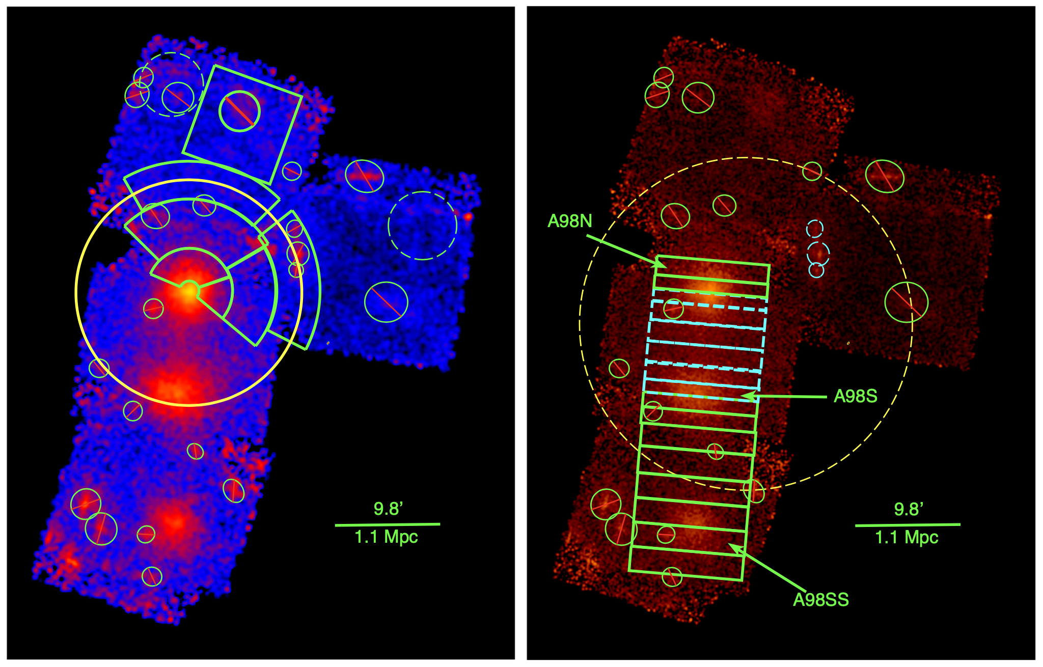
Figure 1: Left: Annotated, mosaic, background subtracted, and exposure corrected Suzaku image of the A98 system in the $0.5-7.0$ keV band. The image is binned to emphasize diffuse features in the system, and smoothed with a 20.8$\arcsec$ Gaussian. The sectors are the regions used for the temperature and entropy profiles for A98N. The yellow circle denotes $r_{\_}{200}$ for A98N derived from the $T_{\_}{500}$-$r_{\_}{500}$ relation found by Vikhlinin et al. (2009). The dashed green circles are regions used to constrain the sky background. The excluded regions are point sources, with the exception of a potential background cluster (see Section 4.2), and are excluded from further analysis. The cyan dashed circle regions mark the point sources that are modelled simultaneously with the outermost sector to the west of A98N. The box region to the north is used to estimate large-scale properties described in Section 4.2. Right: The Suzaku image is smoothed with a 10.4$\arcsec$ circular Gaussian. The box regions are used for the intercluster filament thermodynamic profiles presented in Section 4.2.2. The dashed cyan boxes are used to derive the temperature, electron density, and entropy profile for A98N and A98S presented in Figure 12. The dashed yellow circle denotes the XMM-Newton field of view. The cyan dashed regions and exclusion regions are the same as in the left panel.

The Suzaku data are reduced using HEASOFT version 6.22.1 and the latest calibration database as of May 2014. . The FTOOL aepipeline is used for the first order reprocessing of the unfiltered files. Appropriate filters were applied for an Earth elevation greater than 5^∘, a sunlit Earth elevation greater than 20^∘, a cutoff rigidity greater than 6 GeV/c, and passages just before and after the South Atlantic Anomaly with XSELECT. The 5x5 editing mode files are first converted to the 3x3 editing mode using xis5x5to3x3 and then the events are combined for each detector. The corners of the chips illuminated by the Fe⁵⁵ calibration sources are then removed. The second rows adjacent to the charge injected rows at 6 keV are removed from XIS1 for further analysis due to the increase in NXB level on XIS1. Due to the micrometeorite hit to XIS0, the impacted region is excluded from the XIS0 field throughout the analysis. Light curves are extracted from the events files with the CIAO tool dmextract. The CIAO tool deflare is used on the light curves with the iterative sigma clipping routine lcsigmaclip set to $3\sigma$. No instances of strong flaring in the observations are found.

The non-X-ray background (NXB) images are generated using the xisnxbgen routine (Tawa et al., 2008). The NXB images are then scaled so that the hard-band (10-12 keV) count rate matches the source Suzaku observations. After creating source and scaled NXB mosaic images, the mosaic NXB image is then subtracted from the source image. Flat field images are generated with the routine xissim to create effective exposure maps. to create the final image shown in Figure 1. . The CIAO tool wavdetect is used on wavelet scales of 14, 28, and 56 pixels, where each pixel is $2\arcsec$ in length after binning, to detect point sources. The image was then inspected by eye in order to make appropriate adjustments to the point source regions detected for exclusion from further analysis.

2.2 Chandra

The A98 system was observed with Chandra, with a total of three pointings from September 2009-September 2010 (see Table 2). More recent, deeper Chandra obervations of this system will be presented in Sarkar et al. (in prep). CIAO version 4.9 and CALDB version 4.7.7 are used for the Chandra data reduction. After using chandrarepro to generate level 2 events files (see Table 2 for observations), light curves are extracted with the CIAO tool dmextract, and then run through the deflare routine to filter the level 2 events files for any possible flares during the observation.

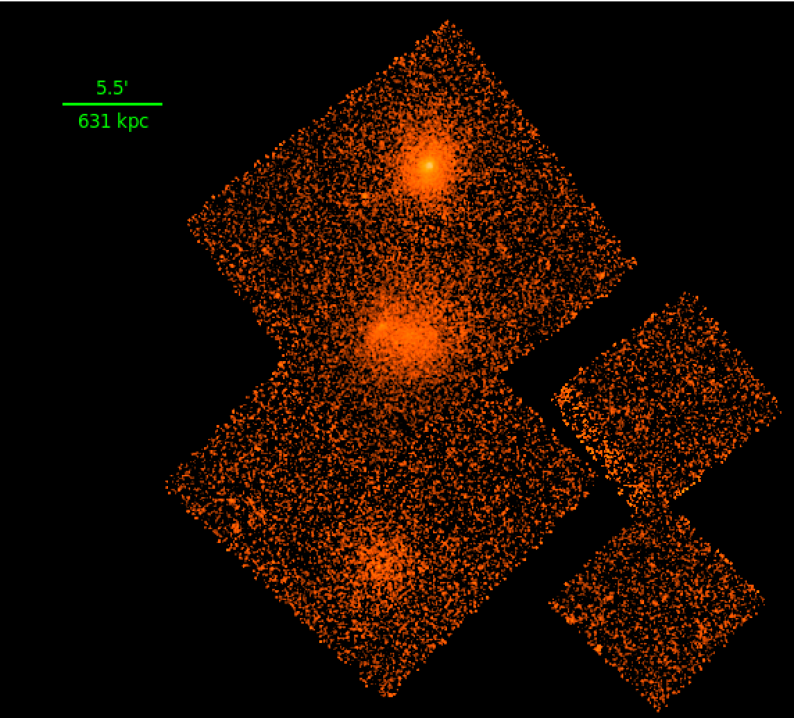
Figure 2: 0.3-7.0 keV blank sky background subtracted, exposure corrected, mosaic image of the Chandra observations (see Table 2). The image is smoothed with a 10″  Gaussian.

The asphist, mkinstmap, and mkexpmap routines in CIAO are used to generate exposure maps for imaging. The blank sky background files with the closest observation periods to each of the Chandra observations are reprojected to match the observations using the CIAO routine reproject_events. The blank sky background images are hard-band (10-12 keV) scaled to match high-energy particle background count rate of the source observations. We use the wavdetect routine on wavelet scales of 2, 4, 6, 8, 10, 12, and 16 pixels, where the pixels are 0.98″ in length to detect background sources for removal. These sources are excluded from further analysis. The routine dmfilth is used to fill in the excluded source regions by drawing counts from a Poisson distribution matched to the local surrounding regions for imaging. The mosaic background subtracted, exposure corrected Chandra 0.3-7.0 keV image is presented in Figure 2.

This Chandra data is used to corroborate Suzaku measurements, and is in general agreement with the deeper observations presented in Sarkar et al. (2022).

2.3 XMM-Newton

The Source Analysis Software (SAS) v18.0.0 is used to reduce the XMM-Newton event lists for A98N. The tools odfingest and cifbuild were used to create summary file and to build a respectively to prepare the data for further analysis. We then use the tool xmmextractor to generate images and calibrated events files for point-like source analysis. A smoothed 0.5-2.0 keV MOS2 image of this observation is presented in Figure 3.

3 Analysis

XSPEC version 12.11.0 was used to perform the spectral analysis. An absorbed (phabs) APEC model (Smith et al., 2001) was used for the source spectra.

3.1 Suzaku Spectroscopy

To extract spectra for the Suzaku observations, the XSELECT environment and subsequently the extract spec routine are utilized. Then the corresponding redistribution matrix file (RMF) is generated with xisrmfgen . The RMF and source spectrum are then used to generate the ancillary response files (ARFs) with xissimarfgen.

Two different ARFs are generated for each spectrum to be folded into two different model components in the spectral fits; the source model and the background model. The Chandra image is used to fit a 2D-$\beta$ model for all three clusters. In order to create more accurate ARFs for the source spectra, xissimarfgen utilizes an image of the 2D-$\beta$ model. A uniform circle with a radius of $20\arcmin$ is used to generate the ARFs folded into the background model, under the assumption that it is uniform.

The background model includes components from the local hot bubble (LHB), the galactic halo (GH) and the cosmic X-ray background (CXB). Non X-ray background (NXB) spectra are generated with xisnxbgen (for more details see (Tawa et al., 2008)) and are subtracted from the source spectra in XSPEC. We group all of our spectra such that each bin contains a minimum of 40 counts. In order to further constrain the GH and LHB, and CXB emission, we extract a spectrum of an annulus from the ROSAT All Sky Survey (RASS). The RASS annulus is centered on RA = $0^{\rm h}46^{\rm m}18^{\rm s}.8872$ and Dec = $20^{\rm h}28^{\rm m}13^{\rm s}.557$, approximately on the X-ray centroid of A98SS, with an inner radius of $0.5643^{\circ}$ and an outer radius of $0.6738^{\circ}$. The free model parameters can be seen in Table 3. The LHB temperature is fixed to $kT=0.1$ keV, and the powerlaw component for the CXB is fixed to $\Gamma=1.4$.

Table 3: The free parameters for the fits to the dashed green background regions shown in Figure 1 (Left).

BG Region	CXB Norm [photons/keV/cm2/s/arcmin2]	GH $kT$ [keV]	GH Norm [cm-5arcmin-2]	LHB Norm [cm-5arcmin-2]
West	$6.9e-7^{+4\rm{e}-8}_{\_}{-4\rm{e}-8}$	$0.19_{\_}{-0.01}^{+0.03}$	$1.3e-6_{\_}{-3\rm{e}-7}^{+8\rm{e}-7}$	$2.1e-7_{\_}{-2\rm{e}-7}^{+1\rm{e}-7}$
North	$6.8e-7^{+3\rm{e}-8}_{\_}{-3\rm{e}-8}$	$0.19_{\_}{-0.02}^{+0.04}$	$1.4e-6_{\_}{-4\rm{e}-7}^{+8\rm{e}-7}$	$1.8e-7_{\_}{-1\rm{e}-7}^{+1\rm{e}-7}$

Most point sources are removed by inspecting the Suzaku, Chandra, and XMM-Newton observations listed in Table 2. The bright point sources that are not excluded from the regions for analysis are modelled simultaneously. We first model the point sources with an absorbed powerlaw model for AGN, and an APEC model for a foreground galactic star, using the XMM-Newton data that overlaps the Suzaku field of view (FOV). We then take the parameters from the model to simulate the same Suzaku point source with the FTOOL xissim. We use this simulation to estimate the Suzaku normalization for the point source models and then fold the point source models into the region fits, allowing the point source parameters to vary within their $90\%$ errors derived from the XMM-Newton fit of the source.

3.1.1 Suzaku Scattered Light

Due to Suzaku’s relatively large PSF, one must consider the effects of scattered light from adjacent regions when performing spectral analysis. In order to determine the effect of scattered light across adjacent regions, we use xissim to simulate each region with $2\times 10^{6}$ photons as is done in e.g. Walker et al. (2012) and Bulbul et al. (2016). We calculate the percentage of photons that originate from the region of interest and are detected in that region, and what percentage of photons are scattered into the adjacent region in order to include a properly weighted component in the spectral fit to the adjacent region (Table 4). We use these values to test whether the scattered light affects our results, particularly in the faintest regions analyzed in this work. We find that the scattered light does not change the final results for the analysis of A98N, as the statistical error dominates the effect of scattered light. We find that the scattered light from outside of the FOV is negligible. Therefore, we omitted values from Table 4 where the adjacent sector was outside of the FOV of the observation containing the source sector.

Table 4: Percentage of light scattered from the regions in the columns into the regions in the rows. “N” represents the sectors to the north of A98N, and “W” represents the sectors to the west of A98N.

Region	N01	N02	N03	W01	W02	W03
N01	65.1	-	-	-	-	-
N02	-	73.2	6.69	-	-	-
N03	-	9.38	70.6	-	-	-
W01	-	-	-	54.5	6.2	-
W02	-	-	-	9.86	60.0	-
W03	-	-	-	-	-	60.7

3.1.2 Systematic Error in the Cosmic X-Ray Background

Suzaku is able to detect point sources down to a flux of $1\times 10^{-13}$ ergs cm^-2 s^-1 deg^-2. Moretti et al. (2003) defines the unresolved CXB flux in ergs cm^-2 s^-1 deg^-2 as

$$F_{\_}{CXB}=(2.18\pm 0.13)\times 10^{-11}-\int_{\_}{S_{\_}{lim}}^{S_{\_}{max}}\frac{dN}{dS}\times S~{}d.$$ (1)

The analytical form of the source flux distribution in the 2-10 keV band is characterized as (Moretti et al., 2003)

$$N(>S)=N_{\_}0\frac{(2\times 10^{-15})^{\alpha}}{S^{\alpha}+S_{\_}0^{\alpha-\beta}S^{\beta}}~{}\rm{ergs}~{}\rm{cm}^{-2}~{}\rm{s}^{-1},$$ (2)

where $\alpha=1.57_{\_}{}^{+0.10}$ and $\beta=0.44^{+0.12}_{\_}{-0.13}$ are the power laws for the bright and faint components of the distribution respectively, $N_{\_}0=5300_{\_}{-1400}^{+2850}$, $S_{\_}{lim}$ is the flux of the faintest point source detected in the observation, and $S_{\_}{max}=8\times 10^{-12}$ ergs cm^-2 s^-1. The nominal value, $S_{\_}{lim}$, for Suzaku point sources is $1\times 10^{-13}$ ergs cm^-2 s^-1 deg^-2 (e.g. Walker et al., 2013). Therefore the unresolved CXB in the background region used in the Suzaku observations has a flux of $1.87\pm$ $\times 10^{-11}$ ergs cm^-2 s^-1 deg^-2.

Finally, the expected $1\sigma$ in the unresolved CXB flux may be given by:

$$\sigma^{2}=\frac{1}{\Omega}\int_{\_}{0}^{S_{\_}{lim}}\frac{dN}{dS}\times S^{2}~{}d$$ (3)

where $\Omega$ is the solid angle (Bautz et al., 2009). We use this method to constrain the normalization of the CXB component of the background, and allow this parameter to vary within the derived $1\sigma$ errors.

3.2 XMM-Newton Spectral Analysis

SAS is used to generate all of the necessary files of the point-like regions shown in Figure 3 for analysis in XSPEC. In order to generate the source and background spectra, we use the evselect routine. We then use the rmfgen routine to generate the redistribution matrix files and the arfgen routine to generate the ancillary response file for the spectrum. The XMM-Newton spectra are grouped such that each bin contains a minimum of 25 counts due to the relatively low counts observed for the point sources. We then use an absorbed powerlaw model in XSPEC for the point sources that are AGN, and a simple APEC model for the point sources that are galactic stars.

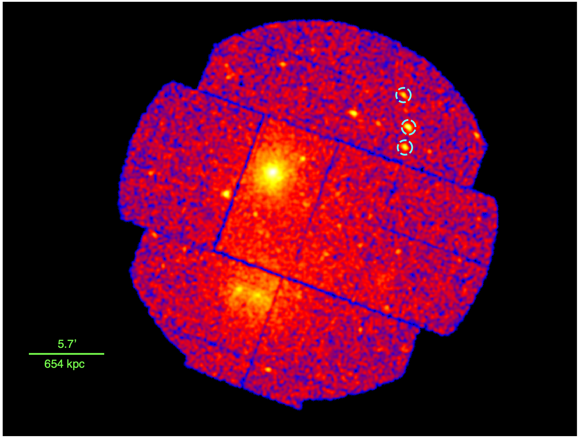
Figure 3: XMM-Newton MOS2 image of A98N and A98S smoothed with a $15\arcsec$ Gaussian kernel. The point sources modelled with XMM-Newton data in this work are highlighted with dashed cyan regions.

4 Results and Discussion

In this section we present temperature, electron density, and entropy profiles for regions shown in Figure 1.

The electron density of regions of interest is derived from the normalization for the APEC model in XSPEC. The electron density may be derived from the XSPEC normalization with the following equation:

$$n_{\_}e=\biggl{[}1.2\ N\times 4.07\times 10^{-10}(1+z)^{2}\\ \biggl{(}\frac{D_{\_}A}{\rm{Mpc}}\biggl{)}^{2}\biggl{(}\frac{V}{\rm{Mpc^{3}}}\biggl{)}^{-1}\biggl{]}^{1/2},$$ (4)

where $D_{\_}A$ is the angular diameter distance to the system, $V$ is the volume for an assumed geometry of the region, $N$ is the XSPEC normalization, and $z$ is the redshift of the object.

4.1 Cluster Thermodynamic Properties

Here we present thermodynamic profiles of the subclusters in the A98 system. In order to deproject our temperature measurements, we use the “onion peeling” method (Ettori et al., 2010) and assume a spherical geometry for the galaxy cluster components in the system.

The Suzaku temperature profile of A98N in partial (see sector regions in e.g. Figure 1 (Left)) is shown in Figure 4 as well as the “Universal” temperature profile (Ghirardini et al., 2019) expected based upon the average electron temperature of the system. While not all of the error constraints are tight, the temperature profile of A98N is not only consistent in partial azimuth, but also seems to adhere to expectations of the temperature profile based on average cluster temperature (cluster $T_{\_}{500}$ measurements with Suzaku are presented in Table 1).

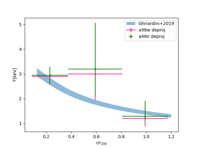
Figure 4: The deprojected temperature profile of A98N for the sectors to the north and west shown in Figure 1. The pink points are for the sectors to the west of A98N and the green points are for the sectors to the north of A98N. The blue line is the “Universal” temperature profile presented in Ghirardini et al. (2019)

The electron density profile of A98N in the northern and western sectors is shown in Figure 5. The profiles are consistent with each other within errors.

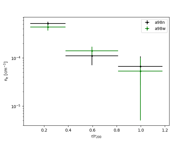
Figure 5: The electron density profile of the annuli to the north and west of A98N (see e.g. Figure 1 (Left))

.

The deprojected entropy profiles for A98N in the northern and western sectors, for the regions shown in e.g. Figure 1 (Left), are shown in Figure 6. Here, entropy is defined as $K=kT_{\_}en_{\_}e^{-2/3}$, where $k$ is Boltzmann’s constant, $T_{\_}e$ is the measured electron temperature, and $n_{\_}e$ is the derived electron density assuming a region appropriate volume as described in Equation 4.

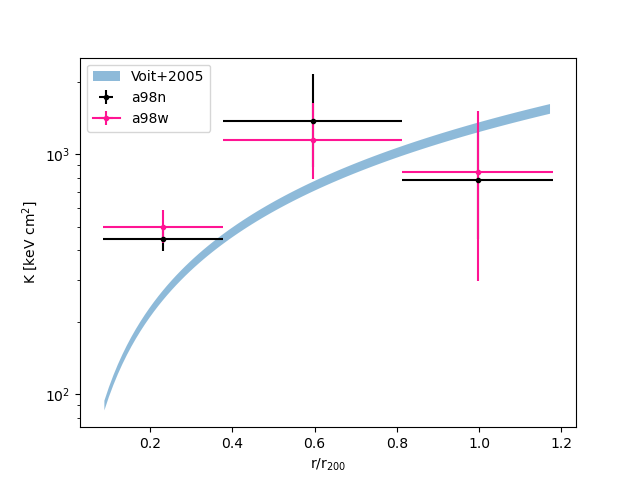
Figure 6: The blue line is the entropy profile expected from pure gravitational collapse (Voit et al., 2005) for A98N. The black points are for the sector regions to the north of A98N and the pink points are for the sector regions to the west of A98N shown in Figure 1.

We find that, in both sectors, the entropy values for A98N are consistent with the self-similar prediction of pure gravitational collapse, , near the virial radius, in which entropy $K\propto r^{1.1}$ (Voit et al., 2005). There is some hint of entropy flattening, however the errors on the entropy are too large to say definitively. This is in agreement with similar studies of lower mass systems (e.g. Su et al., 2015; Bulbul et al., 2016; Sarkar et al., 2021) even though A98N is most likely undergoing a merging event (Paterno-Mahler et al., 2014; Sarkar et al., 2022). At small cluster radii ($r<r_{\_}{500}$), the entropy for A98N is above that expected for self-similarity. This excess is consistent with what is seen in other systems, particularly lower mass systems (Sun et al., 2009), and is likely due to the effect of non-gravitational processes in the central region (e.g. AGN feedback (e.g. O’Sullivan et al., 2011)).

4.2 Large-Scale Filament

The box region to the north of A98N shown in Figure 1 is used to investigate larger-scale structure beyond $r_{\_}{200}$ of A98N. The excluded region within the box does not appear to be a point source, and also does not appear to be associated with the A98 system. Inspecting images from the DSS and SDSS reveals no obvious clustering of galaxies. There are not enough photons available to reliably model the spectrum of this source. This source could be a background galaxy cluster or faint group, although it would require further observations to determine its nature.

This region was fitted with an absorbed APEC model. The best fit values for this box region, excluding the possible background cluster, yield a temperature of assuming a cylindrical volume with length  Mpc and radius of  Mpc, and filling factor of 1 for the density measurement. These values are consistent with the dense end of the WHIM, ,

We compare a similar region to the west, and fit the region with the best fit parameters for the model of the northern region. The fit for the northern box region yields a $\chi^{2}$ of d.o.f. We find that the western comparison region is consistent with background only with a fit that gives a $\chi^{2}$ of d.o.f when the data is fit to the best fit model of the northern region. Such detections of this material are very rare (e.g. Bulbul et al., 2016; Werner et al., 2008). This detection is consistent with the detection of larger-scale structure in the Abell 1750 system, another low mass triple cluster system (Bulbul et al., 2016) similar to A98. With the advent of eRosita and future X-ray missions (e.g. Athena, Lynx), such detections should become more common.

4.2.1 A98N-A98S Bridge

To investigate whether the apparent surface brightness enhancement in between A98N and A98S is due to two cluster halos overlapping, we compare the combined surface brightness profiles of A98N and A98S to the emission across the bridge, as done in (Paterno-Mahler et al., 2014; Sarkar et al., 2022) .

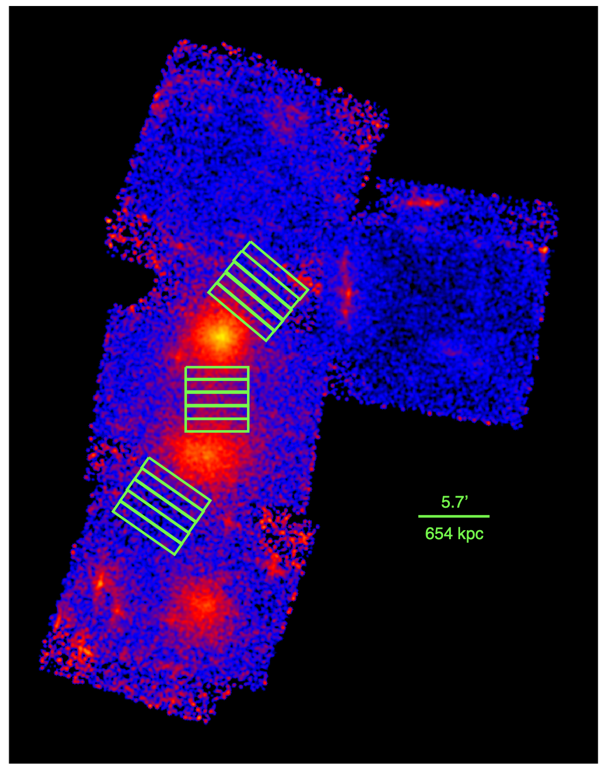
Figure 7: Same as Figure 1: Left, but instead smoothed with a $12.5\arcsec$ Gaussian. The rectangular annuli to the north of A98N and to the south of A98S are used to compare the combined surface brightness of the two clusters to the box regions in the bridge region (see Figure 8).

We combine the background subtracted surface brightness profiles of the box annuli to the north of A98N and to the south of A98S shown in Figure 7. These box annuli are oriented to avoid the large-scale and intercluster filaments in the system. We then compare these values to the surface brightness in the apparent bridge regions connecting A98N and A98S shown in Figure 7.

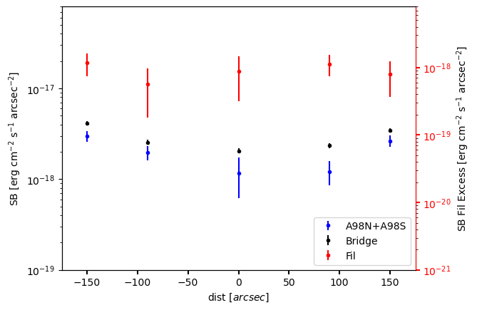
Figure 8: The surface brightness profile with XIS3 in the $0.5-2.0$ keV range, and $1\sigma$ errors for the filamentary region shown in Figure 7 is shown in black points, using the y-axis scale on the left. The corresponding combined rectangular annuli shown in Figure 7 for A98N and A98S are shown for comparison with the blue points. The filament excesses, are shown in red, using the y-axis scale on the right. The zero point on the x-axis is the midpoint of the tentative bridge connecting A98N to A98S.

The combined ICM surface brightness profile as compared to the bridge, and the resulting filament excess is presented in Figure 8 where the zero point on the x-axis is the midpoint of the region connecting A98N and A98S. The emission across the A98N-A98S bridge appears to be slightly enhanced, with a marginal ($2.2\sigma$) detection of excess filament emission. This excess emission is also seen at a higher significance with combined Suzaku and deeper Chandra observations (Sarkar et al., 2022) than are presented in this paper.

4.2.2 Bridge Thermodynamic Properties

We measure the temperature, electron density, entropy, and metallicity across the A98 system with the box regions shown in e.g. Figure 1 (Right). The temperature profile from north to south is shown in Figure 9, and is relatively flat across A98N and A98S before dipping in between A98S and A98SS. When compared to Chandra, the temperature profiles are consistent.

We find that in the intercluster region between A98N and A98S that a two temperature model is preferred (Table 5). We freeze the metallicity at its best fit value found from the one temperature fit, and freeze the metallicity of the second temperature component to $=0.2$ Z${}_{\_}\odot$.

Table 5: Parameters for a 1 temperature and 2 temperature model of the intercluster region between A98N and A98S.

Model	$T_{\_}1$ [keV]	$T_{\_}2$ [keV]	$\chi^{2}$	d.o.f
1T APEC	$2.7_{\_}{-0.2}^{+0.3}$	-	267.3	225
2T APEC	$4.0_{\_}{-1.0}^{+6.5}$	$1.3_{\_}{-0.3}^{+0.3}$	249.9	224

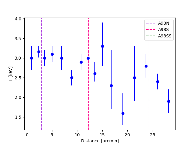
Figure 9: The temperature profile for the box regions across the A98 system shown in Figure 1. The profile starts from the north on the left of the plot. The purple, pink, and green dashed lines mark the center of A98N, A98S, and A98SS respectively.

The inferred electron density (Equation 4) for the regions across the bridge is presented in Figure 10. A cylindrical geometry is assumed for the regions in this profile. Assuming a box geometry for the regions across the bridge yields the same result within errors; therefore neither geometry is preferred. There is a steady decline in the electron density profile with local peaks corresponding to the cluster centers.

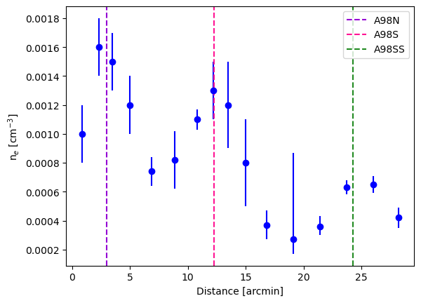
Figure 10: Inferred electron density profile across the A98 system. The profile is starting from the north on the left of the plot. The purple, pink, and green dashed lines mark the center of A98N, A98S, and A98SS respectively.

The metallicity profile across the bridge is shown in Figure 11. This profile suggests that the metallicity of the ICM is radius dependent, with a higher metallicity towards the center of the clusters, and decreases with radius.

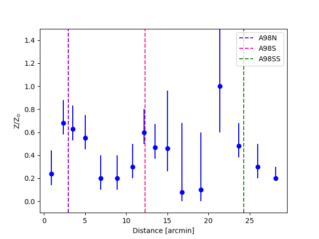
Figure 11: The metallicity profile across the A98 bridge. The profile is starting from the north on the left of the plot. The purple, pink, and green dashed lines mark the center of A98N, A98S, and A98SS respectively.

4.2.3 Filament Orientation

The cyan box regions shown in e.g. Figure 1 (Right) between A98N and A98S can be used to explore the entropy, presumed geometry, and inclination of the system. The entropy profile for the box regions between A98N and A98S is shown in Figure 12. We only include the regions from the center of A98N to the center of A98S in this entropy profile to investigate the filament orientation (cyan regions in e.g. Figure 1 (Right)).

The two extremes for filament orientation: along the line of sight (los) and in the plane of the sky (pos) are investigated (see Figure 12). At the midpoint of the filament, the measured entropy is already approximately the expected ICM value at this radius if the filament is in the pos. This means that either the filament is in the pos, or the entropy of the gas has somehow been increased (e.g., due to a merger shock (Sarkar et al., 2022)). The filament is more likely inclined close to the pos, as a los filament orientation yields entropy values well above what is expected from the self-similar entropy profiles of the clusters (Voit et al., 2005). Furthermore, a line of sight orientation of the system yields entropy values $\sim 2$ times higher than what is expected in the outskirts of both subclusters. These measurements rule out a significant contribution from WHIM emission in this region. The reported entropy values similarly assume a cylindrical geometry for the bridge regions, and assuming a box geometry yields a similar result within errors.

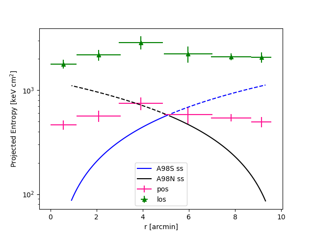
Figure 12: The entropy profile from north to south across the bridge between A98N and A98S. The blue line is the expected universal entropy profile for A98N. The black line is the expected universal entropy profile for A98S. The pink points are the inferred entropy for a filament orientation in the pos. The green triangles are for a filament orientation along the los. A filament orientation closer to the pos is preferred, as the los entropy values are $\sim 2$ times higher than what is expected in the outskirts of both subclusters.

5 Conclusions and Summary

In this paper we present results from an analysis of Suzaku, Chandra and XMM-Newton observations of the diffuse emission in the A98 system.

We find the following:

• The entropy profiles in northern and western sectors, along and away from the merger axis and the putative large scale structure filament, for A98N generally agree with each other, and with the self-similar expectation in the virialization region. This is consistent with previous suggestions (e.g. Su et al., 2015; Bulbul et al., 2016) that lower mass clusters and groups adhere more closely to self-similar expectations in their outskirts, in contrast with what is seen in most massive systems.

• The region to the north of A98N, beyond $r_{\_}{200}$, was found to have a temperature, density, and entropy consistent with those expected for the dense end of the WHIM. We find a temperature of for this region. The presence of similar emission at the same radius to the west, away from the putative large scale structure filament, is ruled out. This serves as further evidence that the system is consistent with the expectation that the merger axis lies along a large-scale structure filament. A similar result was found in the colinear triple system Abell 1750 (Bulbul et al., 2016). These measurements provide tantalizing evidence for the presence of a larger-scale structure, with the diffuse WHIM connecting to the cluster outskirts along cosmic filaments.

• When comparing the surface brightness of the A98N- A98S bridge regions to the combined surface brightness profiles of the two overlapping halos, a nominal $2.2\sigma$ excess in bridge emission is detected. This detection is suggestive of the presence of an intercluster filament in-between the two clusters. Additionally, there is evidence of two-phase plasma in this region; the lower temperature component ($kT\sim 1$ keV) is consistent with the dense end of the WHIM.

• Comparing the entropy profile of the A98N-A98S bridge to that of the self-similar expectations for A98N and A98S reveals that the system is likely inclined closer to the pos. This suggests that the clusters are interacting with each other as they are well within each other’s virial radius in projection.

In this study, a picture similar to the large-scale structure seen in cosmological simulations starts to emerge. Suzaku is a powerful tool for studying diffuse ICM emission at large cluster radii, but is no longer functional and available for future observations. The next generation of X-ray telescopes such as eRosita, XRISM, Athena, and Lynx will provide a wealth of information on the diffuse ICM in the virialization region of galaxy clusters and the surrounding large-scale structure (e.g. Reiprich et al., 2021). The ability to study increasingly low surface brightness cluster outskirt emission will help to answer key questions about the physical processes occurring in these interface regions. This will lead to a new era of synergy between observation and simulation in the pursuit to understand cosmology and the physics that govern the observable Universe.

References

- Abell et al. (1989) Abell, G. O., Corwin, Harold G., J., & Olowin, R. P. 1989, ApJS, 70, 1
- Angelinelli et al. (2021) Angelinelli, M., Ettori, S., Vazza, F., & Jones, T. W. 2021, arXiv e-prints, arXiv:2102.01096
- Avestruz et al. (2015) Avestruz, C., Nagai, D., Lau, E. T., & Nelson, K. 2015, ApJ, 808, 176
- Battaglia et al. (2013) Battaglia, N., Bond, J. R., Pfrommer, C., & Sievers, J. L. 2013, ApJ, 777, 123
- Bautz et al. (2009) Bautz, M. W., Miller, E. D., Sanders, J. S., et al. 2009, PASJ, 61, 1117
- Boehringer & Hensler (1989) Boehringer, H., & Hensler, G. 1989, A&A, 215, 147
- Bregman (2007) Bregman, J. N. 2007, ARA&A, 45, 221
- Bulbul et al. (2016) Bulbul, E., Randall, S. W., Bayliss, M., et al. 2016, ApJ, 818, 131
- Burns et al. (1994) Burns, J. O., Rhee, G., Owen, F. N., & Pinkney, J. 1994, ApJ, 423, 94
- Dolag et al. (2006) Dolag, K., Meneghetti, M., Moscardini, L., Rasia, E., & Bonaldi, A. 2006, MNRAS, 370, 656
- Eckert et al. (2015) Eckert, D., Roncarelli, M., Ettori, S., et al. 2015, MNRAS, 447, 2198
- Ettori et al. (2010) Ettori, S., Gastaldello, F., Leccardi, A., et al. 2010, A&A, 524, A68
- Forman et al. (1981) Forman, W., Bechtold, J., Blair, W., et al. 1981, ApJ, 243, L133
- Fox & Loeb (1997) Fox, D. C., & Loeb, A. 1997, ApJ, 491, 459
- Ghirardini et al. (2019) Ghirardini, V., Eckert, D., Ettori, S., et al. 2019, A&A, 621, A41
- Grevesse & Sauval (1998) Grevesse, N., & Sauval, A. J. 1998, Space Sci. Rev., 85, 161
- Henry et al. (1981) Henry, J. P., Henriksen, M. J., Charles, P. A., & Thorstensen, J. R. 1981, ApJ, 243, L137
- Hoshino et al. (2010) Hoshino, A., Henry, J. P., Sato, K., et al. 2010, PASJ, 62, 371
- Jones & Forman (1999) Jones, C., & Forman, W. 1999, ApJ, 511, 65
- Lau et al. (2009) Lau, E. T., Kravtsov, A. V., & Nagai, D. 2009, ApJ, 705, 1129
- Lovisari et al. (2015) Lovisari, L., Reiprich, T. H., & Schellenberger, G. 2015, A&A, 573, A118
- Mirakhor & Walker (2020) Mirakhor, M. S., & Walker, S. A. 2020, MNRAS, 497, 3204
- Moretti et al. (2003) Moretti, A., Campana, S., Lazzati, D., & Tagliaferri, G. 2003, ApJ, 588, 696
- Nelson et al. (2021) Nelson, D., Springel, V., Pillepich, A., et al. 2021, The IllustrisTNG Simulations: Public Data Release, , , arXiv:1812.05609
- O’Sullivan et al. (2011) O’Sullivan, E., Giacintucci, S., David, L. P., et al. 2011, ApJ, 735, 11