Learning Generic Lung Ultrasound Biomarkers for Decoupling Feature Extraction from Downstream Tasks

Abstract

Contemporary artificial neural networks (ANN) are trained end-to-end, jointly learning both features and classifiers for the task of interest. Though enormously effective, this paradigm imposes significant costs in assembling annotated task-specific datasets and training large-scale networks. We propose to decouple feature learning from downstream lung ultrasound tasks by introducing an auxiliary pre-task of visual biomarker classification. We demonstrate that one can learn an informative, concise, and interpretable feature space from ultrasound videos by training models for predicting biomarker labels. Notably, biomarker feature extractors can be trained from data annotated with weak video-scale supervision. These features can be used by a variety of downstream Expert models targeted for diverse clinical tasks (Diagnosis, lung severity, S/F ratio). Crucially, task-specific expert models are comparable in accuracy to end-to-end models directly trained for such target tasks, while being significantly lower cost to train.

1 Introduction

Medical diagnostics often involve the identification and analysis of various diagnostic indicators called biomarkers that can help understand the underlying pathology to inform patient care. When clinicians interpret point-of-care lung ultrasound (LUS), they identify biomarkers such as A-lines, B-lines, and pleural line thickness and then use these to inform diagnoses and patient care decisions. Training AI networks to specifically identify and classify these biomarkers can both enhance machine learning and render AI outputs to be relatable to clinicians.

Current typical ANN approaches train models end-to-end on the downstream task. By nature of this task specific training, the learnt features are task specific and do not readily generalize to other tasks. [25] These task specific models require retraining or transfer learning to adapt to new end tasks. [23]

We break down the diagnostic learning task into first predicting generic visual biomarkers using weak supervision followed by fitting task specific Expert models on these predicted biomarkers. Decoupling the feature learning from the downstream task enables the model to learn generic features that can readily adapt to new downstream tasks. Our approach of separating the biomarker detection and downstream analysis is analogous to the separation of the human visual cortex and prefrontal cortex of the brain.

The Biomarker detection model is trained to extract general-purpose LUS biomarker feature attributes, representing an entire video with a short vector of highly meaningful features. Compared to typical multi-layer-perceptron (MLP) classifiers that use 2-3 fully-connected (FC) layers, each with 1024-4096 features, our biomarker feature vector is much shorter, currently only 38 scalar values. Each feature carries specific meaning (e.g. the number of B-lines present in the video, which is a good indicator of the severity of the patient). Having such a succinct representation allows easier training of subsequent AI models to perform a variety of end tasks, including future tasks which were not originally anticipated when training the biomarker model. These 38 biomarker features that capture the consolidated view of a video lack any spatial or temporal grounding of these features thus only providing a weak supervision to train the Biomarker model. This problem setup provides some potential benefits highlighted below.

Reduced training cost: The Biomarker model needs to be trained only once and can be easily adapted to any task by training a subsequent expert model on top. The expert model can now be simpler than the biomarker model as it operates on concise biomarker features rather than on image or video space (an extreme dimensionality reduction). Because the expert model is analyzing a much simpler, more apropos representation, it can be trained using less data (with the task-specific labels), whereas more data is needed to train the more complex Biomarker model. Thus the training cost of each expert model is lower. Accordingly, small amounts of patient-specific or task-specific data might be used to create a new AI model by leveraging the biomarker model’s capabilities (which might be learned from a private dataset that was only used to train the biomarker model).

Annotation ease: Human annotators can provide simple, discrete (binary) cues of (presumably) clinically significant features, making no use of tedious segmentation labels, thus reducing the annotation burden. These visual semantic biomarker features are intended to be quickly assignable using binary checkboxes (often as a gestalt observation) by clinical experts. We then leverage weak supervision to ultimately achieve 38 scalar biomarker features.

Interpretable: The predicted biomarkers are relatable to clinicians who can readily understand and verify the Biomarker model’s outputs. This may provide confidence and insight into the immediate inputs of the subsequent diagnostic classification, helping establish trust in the model. We hope our method provides a step towards overall model interpretability. [19]

Causal in nature: By introducing this information bottleneck of training the expert model only on biomarker features, the expert model is limited from overfitting to spurious correlations in the data. [12] took a similar approach to train VAE’s only using a restricted set of input latent variables thus preventing the model from overfitting to confounding variables.

In the rest of the paper, we introduce the biomarker features and show the ease with which our biomarker model can be adapted to diagnostic tasks.

1.0.1 Related Work

Current LUS AI approaches [22, 3, 10] train models directly for the diagnostic end task, sometimes using segmentation labels for pretraining [24, 11] to help improve performance. Although segmentation labels may be thought of as a type of biomarker, segmentations do not succinctly describe the key properties of the videos and segmentation labels are costly to obtain.

The closest prior work may be [8], which annotated video frames to indicate the presence (or absence) of few LUS biomarkers (consolidation, effusion) and trained networks to detect the same. Comparatively, our biomarker features capture a broader range of qualitative characteristics, and our annotated biomarkers are gestalt’ed video features (at low labeling cost) rather than per-frame features, thus providing a weak supervision for model training. We further use these rich but compact biomarker features for diagnostic tasks.

Transfer learning is a popular technique used in the medical domain when working with limited training data, wherein a model trained on cross-domain or cross-modal data is fine-tuned for the intended task. [6, 23] Biomarkers provide a potentially better pretraining task, learning generic features that can be adapted for related downstream tasks.

Contributions Our main technical contribution is (1) the proposed “biomarker” pre-task that helps generalize to pulmonary LUS diagnostic tasks. Other key contributions are: (2) We quantitatively define and classify LUS biomarker features, (3) We believe this to be the first work using ANN models on LUS to predict S/F ratio, and for (4) predicting diverse pulmonary diseases.

2 Methodology

2.0.1 LUS Biomarkers

Merriam-Webster defines a biomarker as “a distinctive biological or biologically derived indicator of a process, event, or condition.” Therefore an ideal biomarker is one that is both sensitive and specific for a disease process. Precise characterization of the set of biomarkers is necessary to optimize the biomarker’s predictive power. For example, A-line count and intensity directly relate to normal lung while B-line count and intensity relate to disease lung. Likewise, pleural indents and breaks are biomarkers of disease. Thus, quantitative labeling of these biomarkers yields better test performance characteristics. To date, a few specific lung ultrasound biomarkers have been described, e.g. the “lung point” for pneumothorax and a sonolucent space between the parietal and visceral pleural surfaces for pleural effusion. [16]

In an effort to capture the qualitative characteristics of LUS diagnostic indicators, we quantitatively define and classify the biomarker features. We categorize the shape, size, location, and quantity of: A-line, B-line, Pleural line thickness & location, Pleural indents & breaks, Consolidation, and Effusion, [16] resulting in 38 (binary) biomarker features (refer to Figure 2 below and to Table 5 in supplementary material for the detailed list of biomarkers). The full list of biomarkers was developed by the authors achieving consensus among the senior clinicians. We recognize that the defined biomarkers aren’t comprehensive and may need to be augmented to better generalize to future diagnostic tasks.

In our experience, the use of an intuitive online quantitative annotator allowed trained sonographers to label and score hundreds of video clips in a fraction of the time that it would take to semantically label these same clips by drawing boundary masks.

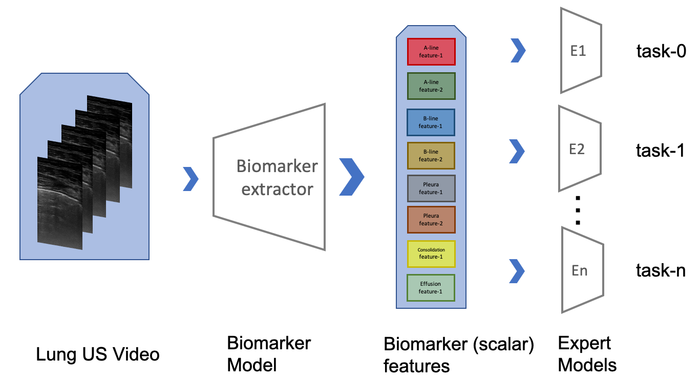
Figure 1: The Biomarker model condenses the video into multi-purpose biomarker feature attributes on which light weight task specific expert models are learnt with no loss in performance.

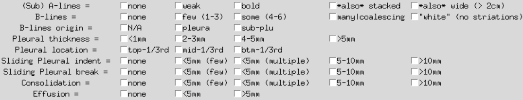
Figure 2: The checkbox annotator used for labeling the 38 biomarkers.

2.1 Data

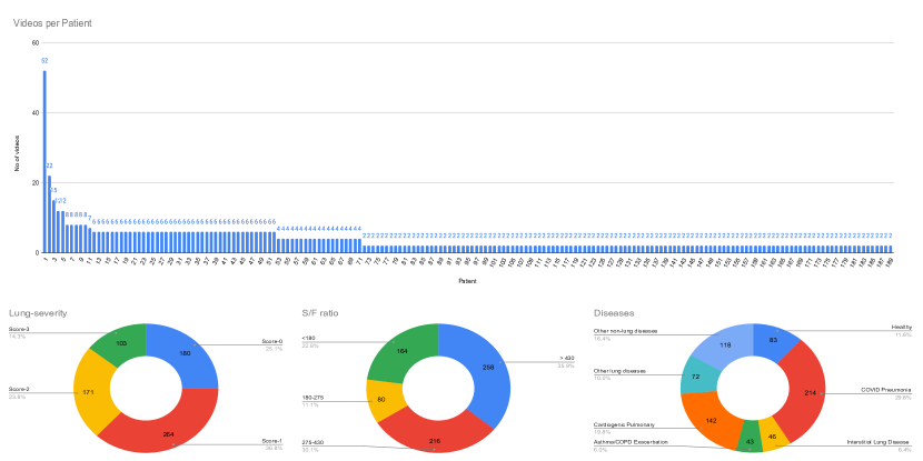
Figure 3: The various dataset distributions. (top) Videos per patient; (bottom) Videos per Lung-severity, S/F ratio, and Disease categories from left to right respectively.

We compiled a lung ultrasound dataset of linear probe videos consisting of 189 patients (718 videos) with multiple (minimum 2 per patient) ultrasound B-scans of left and right lung regions at depths ranging from 4cm to 6cm under different scan settings, obtained using a Sonosite X-Porte ultrasound machine. (Fig. 3 in supplementary material highlights the various dataset distribution.)

Biomarkers: We labeled the 38 binary biomarker features of every video. All the manual labeling was performed by individuals with at least six months of training from a pulmonary ultrasound specialist.

Lung-severity: Each video was scored into 4 lung-severity classes by using the scoring scheme as defined in [1] and similarly used in [22, 10]. The score-0 indicates a normal lung and scores 1 to 3 signify an abnormal lung with increasing level of severity. (Refer to Fig. 4 in supplementary material for sample images corresponding to the severity scores.)

S/F ratio: The S/F represents the ratio between measured blood oxyhemoglobin saturation (S) and the fraction of inspired oxygen (F). The lower this ratio, the more deranged is lung function. S/F is a standardized measurement used to assess lung function in research and at the bedside. We categorize the S/F ratio into the following 4-ranges: $[>430,275-430,180-275,<180]$. These reflect the maximum that the following devices are able to support lungs in oxygenating blood: ambient air, standard nasal cannula, venturi mask, and more intensive oxygen delivery devices only available in intensive care settings (e.g. non-invasive mechanical ventilation, invasive mechanical ventilation) respectively.

Disease: The diagnosis for each patient was recorded and categorised into the following 7-categories: Healthy, COVID Pneumonia, Interstitial Lung Disease, Asthma/COPD Exacerbation, Cardiogenic Pulmonary Edema, Other lung diseases, Other non-lung diseases. These diseases are representative of common pulmonary pathologies encountered in the inpatient clinical setting of an academic American hospital. Each disease imposes disease-specific changes to the physical architecture of lung parenchyma, a property that clinicians use to diagnose pulmonary disease with ultrasound at the bedside.

2.2 Model

We carry out our experiments on the TSM network [17] with ResNet-18 (RN18) [13] backbone and ImageNet [7] pretrained weights. Similar to the setup in [10], we use bi-directional residual shift with $1/8$ channels shifted in both directions. We perform multi-clip evaluation similar to [10] wherein we evaluate n clips (n=4) and the mean prediction across the clips, and use the same frame sampling strategy wherein we feed the model 15 frame inputs selected from 15 equally spaced segments beginning with a random start frame.

The model is trained on images which are resized to 224x224 pixels using bilinear interpolation. We augment the training data using standard augmentations: horizontal flipping, pixel intensity scaling (scales $[0.8,1.1]$), image-scaling ($\pm 20\%$), rotation ($\pm$ 15 degrees), and translation ($\pm$ 5% pixels). The training set is oversampled to address the class imbalance [20].

2.2.1 Classifiers

We use Decision Tree (DT), SVM, Random Forest (RF), AdaBoost (AB), Nearest Neighbours (NN), and MLP classifiers from the scikit-learn python library with default parameters. MLP Large uses 3 hidden layers (128, 64, 32) with adaptive learning rate. To handle the randomness in these simple classifiers we fit 3 models and choose the best model. Similar to the end-to-end trained model, we oversample the training data and perform multi-clip evaluation on the simple classifiers.

2.3 Training Strategy

2.3.1 Implementation

The network is implemented with PyTorch Lightning and trained using the stochastic gradient descent algorithm [4] with an Adam optimizer [15] set with an initial learning rate of $0.0001$, to optimize over cross-entropy loss. The model is trained on an Nvidia RTX A6000 GPU, with a batch size of 4 for 100 epochs. The ReduceLRonPlateau learning rate scheduler is used, which reduces the learning rate by a factor (0.5) when the performance metric (accuracy) plateaus on the validation set. For the final evaluation, we pick the best model with highest validation set accuracy to test on the held-out test set.

Metrics We report accuracy, precision, F1 score [10] and AUC of ROC metrics [14], with weighted average (weights correspond to support of each class) and consider one-vs-one approach for the multi-class classification. [9]

3 Experiments and Results

3.1 Cross-validation

We randomly split the 189 patients into four equal folds, with one fold as the held-out test set (46 patients with 162 videos) and use the other three folds for training by performing 3-fold cross-validation by training on two folds and validating on the other. By creating patient based splits this provides a stricter evaluation (recommended in [21]), although the folds don’t share the same distribution of classes. We report the metrics on the held-out test set in the form of mean and standard deviation over the three independent cross-validation runs.

3.2 Biomarker feature training

We train the biomarker model to predict the 38 biomarker features using binary-cross-entropy loss and use the trained model for the diagnostic tasks by fitting classifier models on top. Refer to Table 4 for biomarker model metrics.

3.3 Diagnostic classification task

We train three task specific models end-to-end (E2E) for lung-severity (4 class), S/F ratio (4 class), and disease category (7 class) classification tasks respectively. We compare the performance of each with the biomarker model (trained once on biomarker feature prediction task) fitted with multiple simple classifiers.

Table 1 shows the mean and standard deviation of the classification metrics obtained from 3-fold cross-validation runs on the independent held-out test set. We observe that the biomarker model achieves comparable performance (often surpassing) the end-to-end trained model on all three diagnostic tasks. By having been trained only once, the Biomarker model ready adapts to different downstream tasks at fractional training cost compared to task-specific end-to-end models, with no loss in performance.

The question that arises now is whether the performance gains of the biomarker model derive from the biomarker features themselves or instead from the different classifier heads (vs. the traditional FC MLP in an ANN). So, we evaluate by fitting simple classifiers on resnet features (from the layer before the last linear classification layer (having 512 embedding size)) of the end-to-end trained model similar to [2, 18]. Although this helps improve the end-to-end model’s performance, it remains subpar to biomarker model’s performance, thus indicative of the effectiveness of biomarker features.

We further evaluated if training an end-to-end model using biomarker pretrained weights improves performance for the lung-severity classification task and observed that it boosts the end-to-end model’s performance and has comparable performance to the biomarker model (refer to section ‘Pretrain on Biomarkers’ of Table 1). We conclude that pretraining on biomarker features provides benefits in both scenarios, whether traditional pretraining or our explicit use by simple Expert models.

In another experiment, we evaluated the transfer-learning/adaptability of the biomarker model by comparing it with the lung-severity end-to-end trained model fit with simple classifiers to predict S/F ratio and Disease categories. We observe (refer to section ‘Lung-severity Features’ of Table 1) that adapting the lung-severity model performs better than the end-to-end trained S/F ratio and disease task models. Yet, this approach sill falls short compared to the biomarker model, suggesting that Biomarker features are more adaptable.

In summary, the Biomarker model generalized better to different diagnostic tasks, and it matched or exceeded the performance of end-to-end trained models.

Table 1: Classification metrics. The biomarker model trained only once for biomarker feature extraction and adapted for diagnostic tasks achieves better performance than directly training end-to-end.

Method	Lung-severity			S/F ratio			Disease		Train Time
	AUC of ROC	Accuracy		AUC of ROC	Accuracy		AUC of ROC	Accuracy	(in min)
End-to-end
E2E	81.5 $\pm$ 1.0	57.6 $\pm$ 2.8		54.6 $\pm$ 4.3	29.6 $\pm$ 1.5		59.2 $\pm$ 1.8	29.2 $\pm$ 2.3	3 x 194
DT	68.2 $\pm$ 2.0	55.6 $\pm$ 2.8		52.9 $\pm$ 2.8	32.1 $\pm$ 5.0		51.8 $\pm$ 2.0	26.5 $\pm$ 1.0	3 x 1
SVM	80.5 $\pm$ 1.9	57.8 $\pm$ 2.3		55.4 $\pm$ 2.5	31.3 $\pm$ 4.7		58.2 $\pm$ 0.4	26.9 $\pm$ 0.8	3 x 1
RF	81.3 $\pm$ 0.2	59.1 $\pm$ 0.8		56.1 $\pm$ 1.7	34.8 $\pm$ 2.5		58.7 $\pm$ 1.0	29.0 $\pm$ 1.3	3 x 2
AB	73.2 $\pm$ 4.8	50.4 $\pm$ 8.6		54.4 $\pm$ 3.2	31.3 $\pm$ 2.9		51.9 $\pm$ 2.8	18.5 $\pm$ 10.3	3 x 2
NN	74.6 $\pm$ 0.7	56.0 $\pm$ 3.0		52.5 $\pm$ 0.9	26.8 $\pm$ 3.6		54.6 $\pm$ 1.7	28.8 $\pm$ 2.8	3 x 1
MLP	80.3 $\pm$ 0.8	59.9 $\pm$ 1.3		54.2 $\pm$ 2.3	32.7 $\pm$ 3.1		57.7 $\pm$ 1.8	29.2 $\pm$ 1.5	3 x 2
MLP large	79.5 $\pm$ 1.7	59.3 $\pm$ 1.8		54.0 $\pm$ 3.1	34.6 $\pm$ 2.0		57.2 $\pm$ 0.8	28.6 $\pm$ 1.8	3 x 3
Biomarker Features									1 x 173.21
DT	68.3 $\pm$ 2.5	54.1 $\pm$ 4.5		55.3 $\pm$ 1.7	35.2 $\pm$ 2.7		53.7 $\pm$ 2.3	24.7 $\pm$ 2.2	3 x 1
SVM	82.9 $\pm$ 1.3	61.3 $\pm$ 2.1		61.7 $\pm$ 2.2	35.8 $\pm$ 4.1		64.2 $\pm$ 3.7	24.1 $\pm$ 1.5	3 x 1
RF	81.2 $\pm$ 1.7	60.3 $\pm$ 3.2		60.5 $\pm$ 2.1	38.5 $\pm$ 1.9		61.2 $\pm$ 3.0	28.4 $\pm$ 0.9	3 x 2
AB	72.7 $\pm$ 2.3	50.8 $\pm$ 2.0		59.3 $\pm$ 3.7	40.3 $\pm$ 4.8		56.2 $\pm$ 3.6	17.9 $\pm$ 5.3	3 x 2
NN	76.2 $\pm$ 3.4	54.1 $\pm$ 2.5		52.8 $\pm$ 2.5	29.0 $\pm$ 3.5		54.5 $\pm$ 5.2	20.8 $\pm$ 3.4	3 x 1
MLP	83.2 $\pm$ 1.4	62.1 $\pm$ 2.0		61.0 $\pm$ 1.7	37.4 $\pm$ 1.3		63.7 $\pm$ 3.5	25.3 $\pm$ 2.0	3 x 2
MLP large	81.6 $\pm$ 0.9	61.1 $\pm$ 1.5		57.4 $\pm$ 1.7	36.6 $\pm$ 4.1		61.1 $\pm$ 4.4	29.2 $\pm$ 1.8	3 x 3
	Pretrain on Biomarkers			Lung-severity Features
E2E	82.4 $\pm$ 2.0	57.4 $\pm$ 0.5							-
DT	68.7 $\pm$ 3.4	57.8 $\pm$ 3.7		56.4 $\pm$ 1.7	37.2 $\pm$ 1.6		53.7 $\pm$ 0.6	22.6 $\pm$ 2.0	3 x 1
SVM	81.9 $\pm$ 2.7	60.5 $\pm$ 3.6		60.2 $\pm$ 1.9	33.5 $\pm$ 2.6		59.3 $\pm$ 2.7	20.2 $\pm$ 2.8	3 x 1
RF	81.6 $\pm$ 3.3	61.1 $\pm$ 2.5		58.2 $\pm$ 1.2	38.9 $\pm$ 2.2		59.4 $\pm$ 1.8	26.1 $\pm$ 2.0	3 x 2
AB	71.2 $\pm$ 3.4	47.9 $\pm$ 13.8		56.8 $\pm$ 3.4	38.3 $\pm$ 3.5		56.6 $\pm$ 1.8	16.9 $\pm$ 4.1	3 x 2
NN	76.5 $\pm$ 2.4	61.1 $\pm$ 0.5		56.4 $\pm$ 0.8	28.8 $\pm$ 3.0		53.7 $\pm$ 3.5	17.5 $\pm$ 2.8	3 x 1
MLP	82.6 $\pm$ 2.3	61.7 $\pm$ 3.6		59.7 $\pm$ 2.6	37.0 $\pm$ 2.0		60.1 $\pm$ 1.7	25.7 $\pm$ 2.0	3 x 2
MLP large	80.6 $\pm$ 2.1	62.6 $\pm$ 2.0		57.9 $\pm$ 2.9	37.2 $\pm$ 2.6		59.5 $\pm$ 1.6	25.9 $\pm$ 1.3	3 x 3

POCOVID Dataset: We next tested the lung-severity models on the 21 linear probe videos in the publicly usable subset of the POCOVID-Net dataset. [3] We observed (refer to Table 4) that the biomarker (Bio) model generalizes better than the end-to-end (E2E) trained model.

Table 2: Biomarker feature model metrics.

Method	Accuracy	Precision	F1-score
Biomarker	76.4 $\pm$ 1.0	70.8 $\pm$ 0.1	73.0 $\pm$ 0.5

Table 3: POCOVID Dataset results.

Method	AUC of ROC	Accuracy
E2E	61.5 $\pm$ 3.2	39.7 $\pm$ 4.5
E2E (SVM)	58.8 $\pm$ 2.0	36.5 $\pm$ 2.2
E2E (MLP)	58.9 $\pm$ 0.7	39.7 $\pm$ 2.2
Bio (SVM)	65.6 $\pm$ 3.1	25.4 $\pm$ 5.9
Bio (MLP)	65.9 $\pm$ 4.1	30.2 $\pm$ 2.2

Table 4: Inter-labeler agreement with LUS Specialist.

Labeler/Model	AUC of ROC	Accuracy
trainee	-	56.79
E2E	75.34	43.21
E2E (SVM)	70.05	46.30
E2E (MLP)	73.70	45.06
Bio (SVM)	76.38	47.53
Bio (MLP)	77.64	49.38

Inter-labeler agreement: We compare the lung-severity model’s predictions and the trainee’s labels (used for training) with labels obtained from an LUS specialist on the test set. We observe (refer to Table 4) the trainee has 56% agreement with the specialist and the biomarker (Bio) model has higher agreement than the end-to-end (E2E) model.

4 Conclusion

Biomarkers can provide improved pre-training and supervision tasks, which helped train a robust lung-ultrasound AI model that can generalize to other tasks. In the future, we would like to incorporate self-supervised training into our biomarker model and to explore ways the model can self-discover interpretable biomarker features rather than pre-specifying them.

Table 5: Biomarkers features (and sub-categories) used in the paper that try to capture the qualitative characteristics of the biomarkers by grouping them into discretized ranges/classes.

Biomarker Feature	Captured qualitative characteristics	Categories
A-line	signifies A-line strength and spread	5
B-line	signifies number of B-lines and type (coalescing or white lung [16])	5
B-line origin	signifies whether B-lines originate at pleura or sub-pleura	3
Pleural line thickness	signifies the thickness of the pleural line	4
Pleural line location	signifies the pleural line location in the image	3
Pleural indents	signifies the indentations in the pleural line	5
Pleural breaks	signifies the breaks in the pleural line	5
Consolidation	signifies the size of consolidation	5
Effusion	signifies the size of effusion	3

Score-0	Score-1	Score-2	Score-3

Figure 4: Sample test set video images corresponding to the four lung-severity classes.

Table 6: Classification metrics using I3D Model. We make use of single stream I3D model [5] with ResNet-50 backbone with Kinetics-400 pretrain weights from PyTorch Moodel Zoo to train the three end-to-end (E2E) models and the biomarker model. We again observe that with the new I3D model architecture, the biomarker model trained only once for biomarker feature extraction and adapted for diagnostic tasks achieves better performance than directly training end-to-end. Highest scores are shown in bold.

Method	Lung-severity			S/F ratio			Disease		Train Time
	AUC of ROC	Accuracy		AUC of ROC	Accuracy		AUC of ROC	Accuracy	(in min)
End-to-end
E2E	81.1 $\pm$ 2.9	57.2 $\pm$ 3.8		56.2 $\pm$ 1.3	34.9 $\pm$ 4.7		59.1 $\pm$ 1.2	24.9 $\pm$ 3.8	3 x 263
Biomarker Features									1 x 256
DT	65.2 $\pm$ 3.6	51.6 $\pm$ 3.4		54.6 $\pm$ 1.5	33.3 $\pm$ 3.8		52.3 $\pm$ 1.5	22.4 $\pm$ 1.3	3 x 1
SVM	82.4 $\pm$ 0.4	58.2 $\pm$ 1.6		61.6 $\pm$ 1.5	36.8 $\pm$ 1.2		64.9 $\pm$ 4.5	26.1 $\pm$ 1.8	3 x 1
RF	81.7 $\pm$ 0.1	60.5 $\pm$ 2.3		61.8 $\pm$ 1.5	40.5 $\pm$ 1.8		65.3 $\pm$ 3.2	30.2 $\pm$ 4.0	3 x 2
AB	71.9 $\pm$ 5.6	48.4 $\pm$ 3.9		56.1 $\pm$ 1.9	34.4 $\pm$ 5.8		59.1 $\pm$ 3.7	20.8 $\pm$ 2.5	3 x 2
NN	72.8 $\pm$ 0.3	51.6 $\pm$ 0.6		54.7 $\pm$ 1.2	31.1 $\pm$ 0.8		58.4 $\pm$ 1.9	23.0 $\pm$ 2.1	3 x 1
MLP	82.8 $\pm$ 1.1	60.7 $\pm$ 1.3		59.9 $\pm$ 0.4	37.4 $\pm$ 2.5		64.2 $\pm$ 3.6	25.7 $\pm$ 1.2	3 x 2
MLP large	80.3 $\pm$ 1.7	61.3 $\pm$ 1.8		57.6 $\pm$ 1.6	36.2 $\pm$ 2.3		62.2 $\pm$ 3.6	27.6 $\pm$ 2.6	3 x 3

Table 7: Detailed classification metrics for the end-to-end (E2E) model and the biomarker model on Lung-severity task (As additional metric for lung-severity task sub-part of Table 1).

Method	AUC of ROC	Accuracy	Precision	F1-score
End-to-end
E2E	81.53 $\pm$ 1.02	57.61 $\pm$ 2.78	58.42 $\pm$ 2.50	57.01 $\pm$ 3.16
DT	68.18 $\pm$ 2.02	55.56 $\pm$ 2.81	55.65 $\pm$ 2.82	55.27 $\pm$ 2.98
SVM	80.53 $\pm$ 1.90	57.82 $\pm$ 2.27	58.46 $\pm$ 2.24	57.47 $\pm$ 1.99
RF	81.28 $\pm$ 0.23	59.05 $\pm$ 0.77	59.52 $\pm$ 0.46	58.41 $\pm$ 0.60
AB	73.17 $\pm$ 4.78	50.41 $\pm$ 8.59	47.47 $\pm$ 10.66	45.07 $\pm$ 11.79
NN	74.58 $\pm$ 0.71	55.97 $\pm$ 3.04	57.06 $\pm$ 3.36	55.97 $\pm$ 3.16
MLP	80.29 $\pm$ 0.78	59.88 $\pm$ 1.33	60.19 $\pm$ 1.59	59.48 $\pm$ 0.94
MLP Large	79.49 $\pm$ 1.71	59.26 $\pm$ 1.82	59.46 $\pm$ 2.06	58.85 $\pm$ 1.37
Biomarker Features
DT	68.26 $\pm$ 2.50	54.12 $\pm$ 4.52	54.55 $\pm$ 4.59	54.12 $\pm$ 4.52
SVM	82.93 $\pm$ 1.32	61.32 $\pm$ 2.10	62.12 $\pm$ 2.14	61.43 $\pm$ 2.06
RF	81.24 $\pm$ 1.73	60.29 $\pm$ 3.24	61.10 $\pm$ 3.15	60.27 $\pm$ 3.27
AB	72.72 $\pm$ 2.27	50.82 $\pm$ 2.04	55.46 $\pm$ 2.53	48.80 $\pm$ 1.26
NN	76.25 $\pm$ 3.36	54.12 $\pm$ 2.49	54.58 $\pm$ 2.14	54.15 $\pm$ 2.34
MLP	83.24 $\pm$ 1.41	62.14 $\pm$ 2.04	62.83 $\pm$ 1.70	62.16 $\pm$ 2.10
MLP Large	81.64 $\pm$ 0.93	61.11 $\pm$ 1.51	62.03 $\pm$ 1.27	61.20 $\pm$ 1.25

References

- [1] Simple, Safe, Same: Lung Ultrasound for COVID-19 - Tabular View - ClinicalTrials.gov, https://clinicaltrials.gov/ct2/show/record/NCT04322487?term=ultrasound+covid&draw=2&view=record
- [2] Almabdy, S., Elrefaei, L.: Deep convolutional neural network-based approaches for face recognition. Applied Sciences (Switzerland) 9(20) (10 2019). https://doi.org/10.3390/APP9204397
- [3] Born, J., Wiedemann, N., Cossio, M., Buhre, C., Brändle, G., Leidermann, K., Aujayeb, A., Moor, M., Rieck, B., Borgwardt, K.: Accelerating Detection of Lung Pathologies with Explainable Ultrasound Image Analysis. Applied Sciences (Switzerland) 11(2) (1 2021). https://doi.org/10.3390/app11020672, https://www.mdpi.com/2076-3417/11/2/672
- [4] Bottou, L.: Large-scale machine learning with stochastic gradient descent. In: Proceedings of COMPSTAT 2010 - 19th International Conference on Computational Statistics, Keynote, Invited and Contributed Papers. pp. 177–186. Springer Science and Business Media Deutschland GmbH (2010). https://doi.org/10.1007/978-3-7908-2604-3_16, https://link.springer.com/chapter/10.1007/978-3-7908-2604-3_16
- [5] Carreira, J., Zisserman, A.: Quo Vadis, action recognition? A new model and the kinetics dataset. In: Proceedings - 30th IEEE Conference on Computer Vision and Pattern Recognition, CVPR 2017. vol. 2017-Janua, pp. 4724–4733 (2017). https://doi.org/10.1109/CVPR.2017.502
- [6] Cheng, D., Lam, E.Y.: Transfer Learning U-Net Deep Learning for Lung Ultrasound Segmentation (10 2021), https://arxiv.org/abs/2110.02196v1
- [7] Deng, J., Dong, W., Socher, R., Li, L.J., Li, K., Fei-Fei, L.: ImageNet: A Large-Scale Hierarchical Image Database http://www.image-net.org.
- [8] Durrani, N., Vukovic, D., Burgt, J.V.D., Antico, M., Sloun, R.J.G.V., Demi, L., Canty, D., Wang, A., Royse, A., Royse, C., Haji, K., Chetty, G., Fontanarosa, D.: Automatic Deep Learning-Based Consolidation / Collapse Classification in Lung Ultrasound Images for COVID-19 Induced Pneumonia Automatic Deep Learning-Based Consolidation / Collapse Classification in Lung Ultrasound Images for COVID-19 Induced Pneumonia (2022). https://doi.org/10.36227/techrxiv.17912387.v1
- [9] Fawcett, T.: An introduction to ROC analysis. Pattern Recognition Letters 27(8), 861–874 (6 2006). https://doi.org/10.1016/j.patrec.2005.10.010
- [10] Gare, G.R., Chen, W., Ling, A., Hung, Y., Chen, E., Tran, H.V., Fox, T., Lowery, P., Zamora, K., Deboisblanc, B.P., Luis Rodriguez, R., Galeotti, J.M.: The Role of Pleura and Adipose in Lung Ultrasound AI . https://doi.org/10.1007/978-3-030-90874-4_14, https://doi.org/10.1007/978-3-030-90874-4_14
- [11] Gare, G.R., Schoenling, A., Philip, V., Tran, H.V., Bennett, P., Rodriguez, R.L., Galeotti, J.M.: DENSE PIXEL-LABELING FOR REVERSE-TRANSFER AND DIAGNOSTIC LEARNING ON LUNG ULTRASOUND FOR COVID-19 AND PNEUMONIA DETECTION (2021)
- [12] Gordaliza, P.M., Vaquero, J.J., Muñoz-Barrutia, A.: Translational Lung Imaging Analysis Through Disentangled Representations. Proceedings of Machine Learning Research-Under Review pp. 1–13 (2022)
- [13] He, K., Zhang, X., Ren, S., Sun, J.: Deep residual learning for image recognition. In: Proceedings of the IEEE Computer Society Conference on Computer Vision and Pattern Recognition. vol. 2016-December, pp. 770–778. IEEE Computer Society (12 2016). https://doi.org/10.1109/CVPR.2016.90, http://image-net.org/challenges/LSVRC/2015/
- [14] Kim, H.E., Kim, H.H., Han, B.K., Kim, K.H., Han, K., Nam, H., Lee, E.H., Kim, E.K.: Changes in cancer detection and false-positive recall in mammography using artificial intelligence: a retrospective, multireader study. The Lancet Digital Health 2(3), e138–e148 (3 2020). https://doi.org/10.1016/S2589-7500(20)30003-0, www.thelancet.com/
- [15] Kingma, D.P., Ba, J.L.: Adam: A method for stochastic optimization. In: 3rd International Conference on Learning Representations, ICLR 2015 - Conference Track Proceedings. International Conference on Learning Representations, ICLR (12 2015), https://arxiv.org/abs/1412.6980v9
- [16] Lichtenstein, D.A.: Current Misconceptions in Lung Ultrasound: A Short Guide for Experts. Chest 156(1), 21–25 (2019). https://doi.org/10.1016/j.chest.2019.02.332, https://doi.org/10.1016/j.chest.2019.02.332
- [17] Lin, J., Gan, C., Han, S.: TSM: Temporal Shift Module for Efficient Video Understanding. Proceedings of the IEEE International Conference on Computer Vision 2019-Octob, 7082–7092 (11 2018), http://arxiv.org/abs/1811.08383
- [18] Lin, T.Y., Roychowdhury, A., Maji, S.: Bilinear CNNs for Fine-grained Visual Recognition http://vis-www.cs.umass.edu/bcnn.
- [19] Lipton, Z.C.: The Mythos of Model Interpretability (6 2016), https://arxiv.org/abs/1606.03490
- [20] Rahman, M.M., Davis, D.N.: Addressing the Class Imbalance Problem in Medical Datasets. International Journal of Machine Learning and Computing pp. 224–228 (2013). https://doi.org/10.7763/ijmlc.2013.v3.307
- [21] Roshankhah, R., Karbalaeisadegh, Y., Greer, H., Mento, F., Soldati, G., Smargiassi, A., Inchingolo, R., Torri, E., Perrone, T., Aylward, S., Demi, L., Muller, M.: Investigating training-test data splitting strategies for automated segmentation and scoring of COVID-19 lung ultrasound imagesa). The Journal of the Acoustical Society of America 150(6), 4118 (12 2021). https://doi.org/10.1121/10.0007272, https://asa.scitation.org/doi/abs/10.1121/10.0007272
- [22] Roy, S., Menapace, W., Oei, S., Luijten, B., Fini, E., Saltori, C., Huijben, I., Chennakeshava, N., Mento, F., Sentelli, A., Peschiera, E., Trevisan, R., Maschietto, G., Torri, E., Inchingolo, R., Smargiassi, A., Soldati, G., Rota, P., Passerini, A., Van Sloun, R.J., Ricci, E., Demi, L.: Deep Learning for Classification and Localization of COVID-19 Markers in Point-of-Care Lung Ultrasound. IEEE Transactions on Medical Imaging 39(8), 2676–2687 (8 2020). https://doi.org/10.1109/TMI.2020.2994459
- [23] Tan, T., Li, Z., Liu, H., Zanjani, F.G., Ouyang, Q., Tang, Y., Hu, Z., Li, Q.: Optimize Transfer Learning for Lung Diseases in Bronchoscopy Using a New Concept: Sequential Fine-Tuning. IEEE Journal of Translational Engineering in Health and Medicine 6 (8 2018). https://doi.org/10.1109/JTEHM.2018.2865787, /pmc/articles/PMC6175035//pmc/articles/PMC6175035/?report=abstracthttps://www.ncbi.nlm.nih.gov/pmc/articles/PMC6175035/
- [24] Xue, W., Cao, C., Liu, J., Duan, Y., Cao, H., Wang, J., Tao, X., Chen, Z., Wu, M., Zhang, J., Sun, H., Jin, Y., Yang, X., Huang, R., Xiang, F., Song, Y., You, M., Zhang, W., Jiang, L., Zhang, Z., Kong, S., Tian, Y., Zhang, L., Ni, D., Xie, M.: Modality alignment contrastive learning for severity assessment of COVID-19 from lung ultrasound and clinical information. Medical Image Analysis 69, 101975 (4 2021). https://doi.org/10.1016/j.media.2021.101975, https://doi.org/10.1016/j.media.2021.101975
- [25] Zech, J.R., Badgeley, M.A., Liu, M., Costa, A.B., Titano, J.J., Oermann, E.K.: Variable generalization performance of a deep learning model to detect pneumonia in chest radiographs: A cross-sectional study. PLOS Medicine 15(11), e1002683 (11 2018). https://doi.org/10.1371/JOURNAL.PMED.1002683, https://journals.plos.org/plosmedicine/article?id=10.1371/journal.pmed.1002683