Hydrodynamic modelling of pulsation period decrease in the Mira–type variable T UMi

Abstract

Pulsation period decrease during the initial stage of the thermal pulse in the helium–burning shell of the Mira–type variable T UMi is investigated with numerical methods of stellar evolution and radiation hydrodynamics. To this end, a grid of evolutionary tracks was calculated for stars with masses on the main sequence $1M_{\sun}\leq M_{\mathrm{ZAMS}}\leq 2.2M_{\sun}$ and metallicity $Z=0.01$. Selected models of AGB evolutionary sequences were used for determination of the initial conditions and the time–dependent inner boundary conditions for the equations of hydrodynamics describing evolutionary changes in the radially pulsating star. The onset of period decrease during the initial stage of the thermal pulse is shown to nearly coincide with the peak helium–burning luminosity. The most rapid decrease of the period occurs during the first three decades. The pulsation period decreases due to both contraction of the star and mode switching from the fundamental mode to the first overtone. The time–scale of mode switching is of the order of a few dozen pulsation cycles. The present–day model of the Mira–type variable T UMi is the first–overtone pulsator with small-amplitude semi–regular oscillations. Theoretical estimates of the pulsation period at the onset of period decrease and the rate of period change three decades later are shown to agree with available observational data on T UMi for AGB stars with masses $1.04M_{\sun}\leq M\leq 1.48M_{\sun}$.

1 Introduction

Variability of T UMi was discovered at the beginning of the twentieth century by Pickering & Fleming (1906) and for a long time this star was known as a long–period Mira–type variable with fairly regular light variations and the period $\Pi\approx 300$ d (Samus’ et al., 2017). This star has attracted the attention after reports by Gal & Szatmary (1995) and Mattei & Foster (1995) on significant decrease of the pulsation period which has begun in 1970s when its period of light variations was $\Pi\approx 315$ d. The authors of these papers supposed that observed period decrease is due to the star contraction during the initial stage of the thermal pulse in the helium burning shell (Wood & Zarro, 1981). Observational estimates of the period change rate obtained from parabolic fits of the $O-C$ diagram spanning two decades are $\dot{\Pi}\approx-3.5$ d/yr (Smelcer, 2002) and $\dot{\Pi}\approx-3.8$ d/yr (Szatmáry et al., 2003). In 2001 the period of T UMi was $\Pi\approx 230$ d and afterwards the fairly periodic oscillations changed to semi–regular light variations with possible switch from the fundamental mode to the first overtone (Uttenthaler et al., 2011). In more detail observations of T UMi are duscussed by Molnár et al. (2019).

The date of the onset of pulsation period decrease in T UMi is known with accuracy about 10 yr so that this star is of great interest because of an opportunity to obtain constraints on the mass of the AGB star. However, only two theoretical studies devoted to evolution and pulsations of T UMi have been done so far. Fadeyev (2018) computed the grid of non–linear pulsation models of red giants with initial conditions obtained from evolutionary sequences of AGB–stars with masses on the main sequence $1M_{\sun}\leq M_{\mathrm{ZAMS}}\leq 2M_{\sun}$. He found that the mass of T UMi is $M=0.93M_{\sun}$. Molnár et al. (2019) undertook a linear analysis of stellar pulsations in red giants also based on stellar evolution calculations and their estimate of the mass of T UMi is $M=1.66M_{\sun}$.

Though the authors of both works used the Bloecker (1995) mass loss rate formula, Fadeyev (2018) carried out evolutionary calculations with parameter $\eta_{\mathrm{B}}=0.05$ whereas Molnár et al. (2019) used the value $\eta_{\mathrm{B}}=0.1$. Below we show that evolutionary calculations of the AGB stage with mass loss parameter in the range $0.02\leq\eta_{\mathrm{B}}\leq 0.1$ allow us to obtain hydrodynamic models reproducing period decrease observed during several decades in T UMi notwithstanding the fact that their stellar masses range from $1.04M_{\sun}$ to $1.48M_{\sun}$. Therefore, the existing observational data on T UMi are insufficient for accurate determination of the stellar mass. One should also bear in mind that the mass loss rates of AGB stars remain highly uncertain (Willson, 2000; Höfner & Olofsson, 2018).

Another cause of uncertainties in estimates of the stellar mass obtained by Fadeyev (2018) and Molnár et al. (2019) is due to the assumption that the initial model of the stellar envelope used for computations of stellar pulsations is assumed to be in thermal equilibrium. As we show below, this assumption appropriate in studies of Cepheids or RR Lyr stars becomes wrong in the case of significant deviation from thermal equilibrium in the contracting envelope of the AGB star undergoing a thermal pulse in the helium–burning shell.

The goal of the present study is to diminish the role of uncertainties mentioned above. First, the evolutionary sequences of AGB stars are calculated with different values of the mass loss parameter $\eta_{\mathrm{B}}$ in order to evaluate dependence of the theoretical estimate of the stellar mass on the mass loss rate. Second, the equations of radiation hydrodynamics are solved with time–dependent inner boundary conditions obtained from evolutionary calculations so that the hydrodynamic model is fully consistent with evolutionary changes in the stellar envelope. This method is appropriate for calculating the non–linear pulsations of stars with significant deviation from thermal equilibrion and has earlier been used for explanation of decaying oscillations in the type–II Cepheid RU Cam (Fadeyev, 2021). Hydrodynamic models of TU UMi presented below reproduce evolutionary changes in stellar pulsations for the time interval $\loa 120$ yr after the onset of period decrease.

2 Evolutionary sequences of AGB stars

Initial conditions for solution of the equations of hydrodynamics were determined on the basis of evolutionary computations for stars with masses on the main sequence $1M_{\sun}\leq M_{\mathrm{ZAMS}}\leq 2.2M_{\sun}$. The initial fractional abundances of helium and heavier elements were assumed to be $Y=0.28$ and $Z=0.01$, respectively. Stellar evolution was computed with the program MESA version 15140 (Paxton et al., 2019). Convection was treated according to the standard mixing–length theory (Böhm-Vitense, 1958) with mixing length to pressure height ratio $\alpha=1.8$. The extended convective mixing was treated according to the exponential diffusive overshoot method (Herwig, 2000) with parameter $f_{\mathrm{ov}}=0.014$. Energy generation rates and nucleosynthesis were computed using the nuclear reaction network consisting of 26 isotopes from hydrogen ${}^{1}\textrm{H}$ to magnesium ${{}^{24}}\textrm{Mg}$. The rates of 81 reactions were calculated with the database REACLIB (Cyburt et al., 2010).

Mass loss rates at evolutionary stages preceding AGB were evaluated by the (Reimers, 1975) formula using the parameter $\eta_{\mathrm{R}}=0.5$. We assumed that the AGB stage begins when the central helium abundance is $Y_{\mathrm{c}}\leq 10^{4}$. Calculations of AGB stellar evolution were done for three different values of the mass loss rate parameter ($\eta_{\mathrm{B}}=0.02$, 0.05, 0.1) of the Bloecker (1995) formula so that three evolutionary sequences of the AGB stage were computed for each value of the initial stellar mass $M_{\mathrm{ZAMS}}$.

In the present study we assumed that the onset of period decrease coincides with the maximum of the helium–burning luminosity $L_{3\alpha}$. The applicability of this approximation is illustrated in Fig. 1, where the helium–burning luminosity (top panel) and the radius of the evolving star (bottom panel) are shown as a function of time $t_{\textrm{ev}}$ for evolutionary sequences $M_{\mathrm{ZAMS}}=1.3M_{\sun}$, $\eta_{\mathrm{B}}=0.02$, $i_{\textrm{TP}}=8$ and $M_{\mathrm{ZAMS}}=1.7M_{\sun}$, $\eta_{\mathrm{B}}=0.05$, $i_{\textrm{TP}}=10$. Here $i_{\textrm{TP}}$ is the number of the thermal pulse and the time $t_{\textrm{ev}}$ is set to zero at the maximum of $L_{3\alpha}$. As seen in Fig. 1, the radius commences to decrease within a time interval $0\la t_{\textrm{ev}}\la 10$ yr. Because the pulsation period and the radius relate as $\Pi\propto r^{3/2}$ we can conclude that this time interval is comparable with observational uncertainty of the onset of period decrease in T UMi.

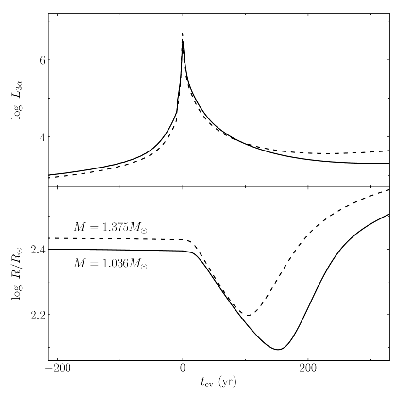
Figure 1: Time dependence of the helium–burning luminosity $L_{3\alpha}$ (top panel) and the stellar radius $R$ for evolutionary sequences $M_{\mathrm{ZAMS}}=1.3M_{\sun}$, $\eta_{\mathrm{B}}=0.02$, $i_{\textrm{TP}}=8$ (solid lines) and $M_{\mathrm{ZAMS}}=1.7M_{\sun}$, $\eta_{\mathrm{B}}=0.05$, $i_{\textrm{TP}}=10$ (dashed lines). The stellar mass $M$ is indicated at the plots.

To measure the deviation from thermal equilibrium in the spherically symmetric stellar envelope we used the parameter $\delta_{\mathrm{L}}=|1-L_{N}/L_{0}|$, where $L_{0}$ and $L_{N}$ are the luminosities at the innermost and the uppermost mass zones of the stellar envelope model, respectively. Envelopes of evolutionary models with age $t_{\textrm{ev}}\leq 0$ were found to insignificantly deviate from thermal equilibrium ($\delta_{\mathrm{L}}\loa 0.02$) so that the non–linear pulsation model can be computed with the time–independent inner boundary conditions

$$\dfrac{\partial r_{0}}{\partial t}=\dfrac{\partial L_{0}}{\partial t}=0.$$ (1)

To compute the limit–cycle pulsation models, we solved the Cauchy problem for the equations of radiation hydrodynamics (Fadeyev, 2015) and time–dependent turbulent convection (Kuhfuss, 1986). The model of the stellar enevelope selected for calculation of initial conditions was divided into 600 zones with the innermost zone at the radius $r_{0}\approx 2\times 10^{-3}R$, where $R$ is the radius of the outer boundary. The mass intervals of 500 outer zones increase geometrically inwards whereas the mass intervals of 100 inner zones decrease. The use of smaller mass intervals at the bottom of the envelope is necessary to obtain a better approximation in the inner layers of the stellar envelope with rapidly increasing pressure and temperature gradients.

Regular radial pulsations of red giants exist in the form of the standing wave with the open outer boundary so that the kinetic energy of pulsation motions $E_{\mathrm{K}}$ reaches the maximum twice per period. Fig. 2 shows the maxima of $E_{\mathrm{K}}$ as a function of time for the model of the evolutionary sequence $M_{\mathrm{ZAMS}}=1.8M_{\sun}$, $\eta_{\mathrm{B}}=0.1$, $i_{\textrm{TP}}=11$ with pulsation period $\Pi^{*}=312$ d. Calculations of initial conditions were finished after attainment of the limit–cycle oscillations. The pulsation period $\Pi^{*}$ of the model with age $t_{\textrm{ev}}=0$ was evaluated using the discrete Fourier transform of the kinetic energy of pulsation motions $E_{\mathrm{K}}$ at the stage of limit–cycle oscillations.

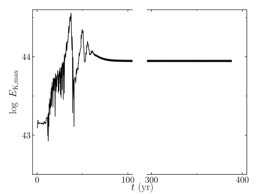
Figure 2: The maximum kinetic energy $E_{\mathrm{K,max}}$ as a function of time $t$ during amplitude growth and limit–cycle oscillations of the model $M_{\mathrm{ZAMS}}=1.8M_{\sun}$, $\eta_{\mathrm{B}}=0.1$, $i_{\textrm{TP}}=11$.

3 Hydrodynamic models

In this work we selected 26 evolutionary sequences with different values of $M_{\mathrm{ZAMS}}$, $\eta_{\mathrm{B}}$ and $i_{\textrm{TP}}$ for calculation of hydrodynamic models. Their pulsation periods at the peak helium–burning luminosity range between 262 d and 365 d. The initial conditions for calculating the hydrodynamic models were determined using the non–linear limit–cycle pulsation models with the age $-200~{}\textrm{yr}\loa t_{\textrm{ev}}\loa-100~{}\textrm{yr}$. Deviation from thermal equilibrium in the evolutionary model of the stellar envelope is $\delta_{\mathrm{L}}<10^{-3}$ so that calculations of limit–cycle stellar oscillations were performed in the manner described in the previous section.

3.1 Inner boundary conditions

Calculation of the hydrodynamic model implies that the time–independent inner boundary conditions (1) are replaced by the time–dependent inner boundary conditions $r_{0}(t_{\textrm{ev}})$, $L_{0}(t_{\textrm{ev}})$ determined from evolutionary calculations for the Lagrangean coordinate of the innermost mass zone. An example of time–dependent inner boundary conditions is displayed in two upper panels of Fig. 3. The plots of $T_{0}$ and $R$ in two lower panels show time dependences of the temperature at the innermost mass zone and the radius of the evolutionary model.

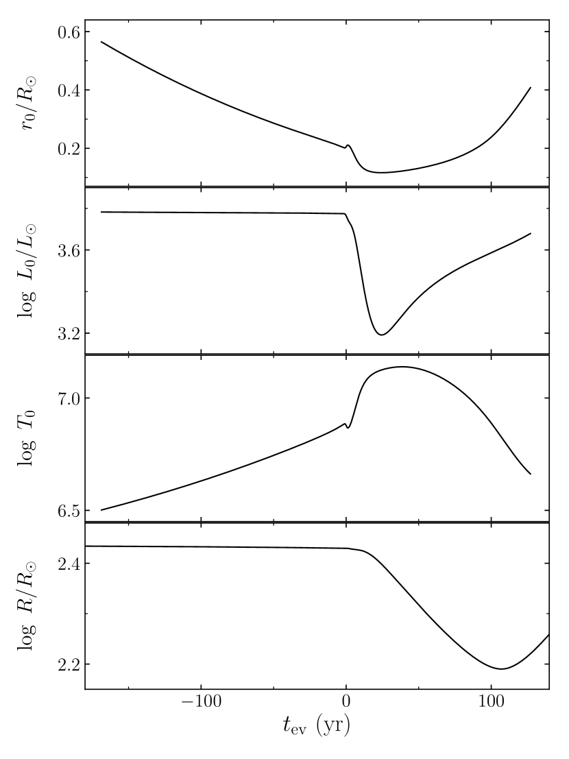
Figure 3: Time dependence of the radius $r_{0}$, the luminosity $L_{0}$ and the temperature $T_{0}$ at the innermost mass zone of the hydrodynamic model $M_{\mathrm{ZAMS}}=1.8M_{\sun}$, $\eta_{\mathrm{B}}=0.1$, $i_{\textrm{TP}}=11$. In the bottom panel, the radius $R$ of the evolutionary model as a function of the age $t_{\textrm{ev}}$.

In the present study we assumed that no convection occurred at the inner boundary so that the innermost mass zone should be always deeper than the bottom of the outer convection zone. Rapid decrease of the temperature $T_{0}$ for $t_{\textrm{ev}}>30$ yr (see Fig. 3) is accompanied by inward movement of the bottom of the outer convection zone. Hydrodynamic calculations are carried out only until the bottom of the convection zone reaches the inner boundary of the model. As seen in the lower panel of Fig. 3, our method of calculations allows us to consider the whole stage of stellar radius decrease as well as the initial stage of subsequent expansion of the star.

3.2 Evolution of stellar pulsations

The solution of the equations of hydrodynamics with time–dependent inner boundary conditions is almost fully consistent with calculations of stellar evolution. The only exception is that the hydrodynamic computations are done for the model with the constant mass. However at the end of hydrodynamic computations the difference between masses of the evolutionary and hydrodynamic models is less than $\sim 0.03\%$ so that effects of mass loss in hydrodynamic computations can be neglected.

In Fig. 4 we show the minimum and maximum radii of the pulsating star for hydrodynamic models $M_{\mathrm{ZAMS}}=1.3M_{\sun}$, $\eta_{\mathrm{B}}=0.02$, $i_{\textrm{TP}}=8$ and $M_{\mathrm{ZAMS}}=1.7M_{\sun}$, $\eta_{\mathrm{B}}=0.02$, $i_{\textrm{TP}}=14$. At the age $t_{\textrm{ev}}=0$ the mass of the star, the pulsation period and the relative amplitude at the upper boundary are $M=1.036M_{\sun}$, $\Pi^{*}=311$ d, $\delta R/R\approx 0.76$ and $M=1.458M_{\sun}$, $\Pi^{*}=330$ d, $\delta R/R\approx 0.61$, respectively. Decline of the pulsation amplitude during contraction of the star is due to decrease of the mass of the hydrogen ionization zone accompanying temperature increase in the stellar envelope.

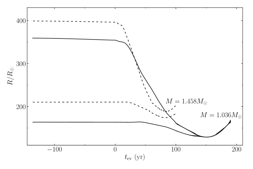
Figure 4: Time dependence of the minimum and maximum radii of hydrodynamic models $M_{\mathrm{ZAMS}}=1.3M_{\sun}$, $\eta_{\mathrm{B}}=0.02$, $i_{\textrm{TP}}=8$ (solid lines) and $M_{\mathrm{ZAMS}}=1.7M_{\sun}$, $\eta_{\mathrm{B}}=0.02$, $i_{\textrm{TP}}=14$ (dashed lines). Masses of hydrodynamic models are given near the curves.

The pulsation period of the hydrodynamic model $\Pi(t_{\textrm{ev}})$ was evaluated for each cycle of pulsations as a time interval between two adjacent maxima of the radius of the outer boundary. The temporal dependence of the period for the hydrodynamic model $M_{\mathrm{ZAMS}}=1.8_{\sun}$, $\eta_{\mathrm{B}}=0.10$, $i_{\textrm{TP}}=11$ is shown in the upper panel of Fig. 5. The gap in the plot corresponds to switch of oscillations from the fundamental mode ($f_{0}$) to the first overtone ($h_{1}$) when evaluation of the period becomes impossible because of a beat phenomenon.

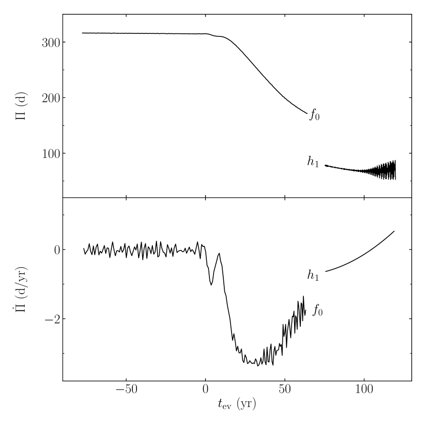
Figure 5: The time dependence of the pulsation period $\Pi$ (upper panel) and the rate of period change $\dot{\Pi}$ (lower panel) for the hydrodynamic model $M_{\mathrm{ZAMS}}=1.8_{\sun}$, $\eta_{\mathrm{B}}=0.10$, $i_{\textrm{TP}}=11$. Plots labelled as $f_{0}$ and $h_{1}$ correspond to pulsations in the fundamental mode and in the first overtone, respectively.

In the lower panel of Fig. 5 we show the time dependence of the rate of period change $\dot{\Pi}$. For the time interval with fundamental mode pulsations the period change rate was evaluated by differentiation of the Lagrange second degree interpolating polynomial and the scatter of individual estimates of $\dot{\Pi}$ is due to the fact that radial pulsations are not perfectly periodic. At the same time, we did not succeed to calculate in the same manner $\dot{\Pi}(t_{\textrm{ev}})$ for oscillations in the first overtone because of increasing scatter of individual estimates of the period (see the plot $h_{1}$ in the upper panel of Fig. 5). In the following subsection we will show that this is due to increasing amplitude of the fundamental mode. Rough estimates of $\dot{\Pi}$ shown in the lower panel of Fig. 5 by the smooth line were obtained by differentiation of the 3rd order algebraic polynomial approximating the time dependence $\Pi(t_{\textrm{ev}})$ labelled in the upper panel as $h_{1}$.

The most conspicuous feature of the plot labelled as $f_{0}$ in the lower panel of Fig. 5 is the deep minimum of $\dot{\Pi}(t_{\textrm{ev}})$ indicating that the most rapid period decrease takes place during a few decades after maximum of the helium–burning luminosity. In Fig. 6 we show the plots of $\dot{\Pi}(t_{\textrm{ev}})$ for three hydrodynamic models with periods at the maximum helium–burning luminosity $\Pi^{*}=262$ d, 314 d and 365 d. These models were computed for three different evolutionary sequences: $M_{\mathrm{ZAMS}}=1.6_{\sun}$, $\eta_{\mathrm{B}}=0.10$, $i_{\textrm{TP}}=7$, $M_{\mathrm{ZAMS}}=1.4_{\sun}$, $\eta_{\mathrm{B}}=0.02$, $i_{\textrm{TP}}=9$ and $M_{\mathrm{ZAMS}}=2.2_{\sun}$, $\eta_{\mathrm{B}}=0.10$, $i_{\textrm{TP}}=19$, respectively. Estimates of $\dot{\Pi}$ minima were obtained by polynomial approximation (dashed lines) and are shown by filled circles. Among 26 hydrodynamic models with periods $262~{}\textrm{d}\leq\Pi^{*}\leq 365~{}\textrm{d}$ we found that the highest rate of period decrease $\dot{\Pi}_{\mathrm{min}}$ as well as the time corresponding to this minimum $t_{\textrm{ev}}(\dot{\Pi}_{\mathrm{min}})$ depend only on the the value of period $\Pi^{*}$.

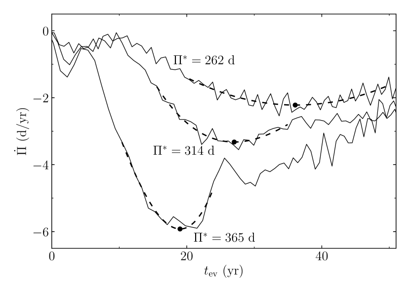
Figure 6: The rate of period change as a function of time for hydrodynamic models with period at the maximum helium–burning luminosity $\Pi^{*}=262$ d, 314 d and 365 d. Dashed lines show the polynomial approximation of the minimum of $\dot{\Pi}$. Filled circles represent estimates of the highest rate of period decrease.

Table 1 lists properties of eight hydrodynamic models with periods $\Pi^{*}$ different from the value 315 d by less than 5% so that below they are referred as hydrodynamic models of T UMi. The second and the third columns give the values of the highest rate of period decrease $\dot{\Pi}_{\mathrm{min}}$ and of the corresponding evolution time $t_{\textrm{ev}}(\dot{\Pi}_{\mathrm{min}})$. Columns labelled as $\Pi_{0}$ and $\Pi_{1}$ give the periods of the fundamental mode and of the first overtone evaluated by extrapolation of dependences $f_{0}$ and $h_{1}$ with respect to $t_{\textrm{ev}}$ into the central point of the gap. It should be noted that the period ratios $\Pi_{1}/\Pi_{0}$ given in the sixth column agree well with estimates obtained from the linear theory (Fox & Wood, 1982; Xiong & Deng, 2007; Molnár et al., 2019). In the seventh column we give the mass of the hydrodynamic model $M$ and in the last three columns we provide the values of $M_{\mathrm{ZAMS}}$, $\eta_{\mathrm{B}}$ and $i_{\textrm{TP}}$.

Table 1: Hydrodynamic models of T UMi.

$\Pi^{*}$	$\dot{\Pi}_{\mathrm{min}}$	$t_{\textrm{ev}}(\dot{\Pi}_{\mathrm{min}})$	$\Pi_{0}$	$\Pi_{1}$	$\Pi_{1}/\Pi_{0}$	$M$	$M_{\mathrm{ZAMS}}$	$\eta_{\mathrm{B}}$	$i_{\textrm{TP}}$
d	d/yr	yr	d	d		$M_{\sun}$	$M_{\sun}$
311	-3.31	31.1	142	71	0.500	1.04	1.3	0.02	8
312	-3.28	29.5	164	82	0.500	1.32	1.8	0.10	11
314	-3.35	26.9	150	75	0.500	1.14	1.4	0.02	9
318	-3.37	29.2	174	88	0.506	1.38	1.7	0.05	10
318	-3.20	31.4	151	75	0.497	1.24	1.5	0.02	10
320	-3.50	30.7	169	85	0.503	1.36	1.6	0.02	11
321	-3.18	31.8	170	85	0.500	1.39	1.6	0.02	10
325	-3.83	28.4	177	91	0.514	1.48	2.0	0.10	16

A cursory glance at Table 1 reveals that all hydrodynamic models insignificantly differ from each other in values of $\dot{\Pi}_{\mathrm{min}}$ and $t_{\textrm{ev}}(\dot{\Pi}_{\mathrm{min}})$. Moreover, the average values $\langle\dot{\Pi}_{\mathrm{min}}\rangle\approx-3.4$ d/yr and $\langle t_{\textrm{ev}}(\dot{\Pi}_{\mathrm{min}})\rangle\approx 30$ yr are in good agreement with observational estimates $\dot{\Pi}\approx-3.5$ d/yr (Smelcer, 2002) and $\dot{\Pi}\approx-3.8$ d/yr (Szatmáry et al., 2003) obtained nearly 30 yr after the onset of period decrease. Thus, the mass of T UMi seems to be in the range $1.04\leq M/M_{\sun}\leq 1.48$.

More rigorous constraint on the mass can be obtained when cessation of period decrease is detected observationally. Dependence of the duration of period decrease on the stellar mass is illustrated in Fig. 7 where the plots of the period as a function of time $t_{\textrm{ev}}$ are shown for three hydrodynamic models with different stellar masses. The minimum of the period is achieved when the star is the first overtone pulsator whereas the duration of period decrease ranges from $\approx 85$ yr for $M=1.48M_{\odot}$ to $\goa 150$ yr for $M=1.04M_{\odot}$.

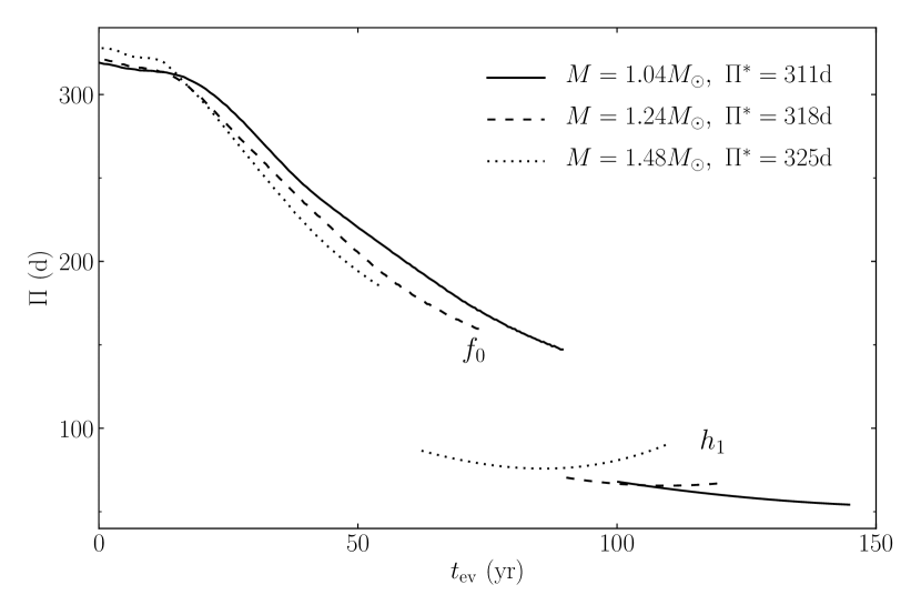
Figure 7: The pulsation period as a function of time for three hydrodynamic models listed in Table 1.

In conclusion of this subsection, it is to be noted that as soon as the deviation from thermal equilibrium in the pulsating envelope becomes appreciably large ($\delta_{\mathrm{L}}\goa 0.1$) the use of the time–dependent inner boundary conditions leads to results that significantly differ from those obtained with (1). For example, deviation from thermal equilibrium in the envelope of the model of the evolutionary sequence $M_{\mathrm{ZAMS}}=1.8M_{\sun}$, $\eta_{\mathrm{B}}=0.1$, $i_{\textrm{TP}}=11$ with age $t_{\textrm{ev}}=30$ yr is $\delta_{\mathrm{L}}=0.23$. The use of this model as initial conditions for calculations of self–excited nonlinear stellar oscillations with time–independent inner boundary conditions leads to the limit cycle solution in the form of the first overtone pulsator with period $\Pi=108$ d. However, as seen in Fig. 5, the hydrodynamic model with age $t_{\textrm{ev}}=30$ yr is still the fundamental mode pulsator with period $\Pi\approx 260$ d.

3.3 Pulsational mode switching

Solution of the equations of hydrodynamics with time–dependent inner boundary conditions allowed us to trace mode switching in the contracting stellar envelope. This is illustrated in Fig. 8 where the radius of the outer boundary of the hydrodynamic model $M_{\mathrm{ZAMS}}=1.8M_{\sun}$, $\eta_{\mathrm{B}}=10$, $i_{\textrm{TP}}=11$ is shown as a function of time $t_{\textrm{ev}}$. Mode switching from the fundamental mode to the first overtone occurs in the time interval $30~{}\textrm{yr}\loa t_{\textrm{ev}}\loa 70~{}\textrm{yr}$. The period ratio of the first overtone and the fundamental mode is $\Pi_{1}/\Pi_{0}\approx 0.50$ (see Table 1) so that mode switching is seen as the gradually increasing bump between two adjacent maxima of the radius. All hydrodynamic models show the similar behaviour and the only difference is the age at the onset of mode switching.

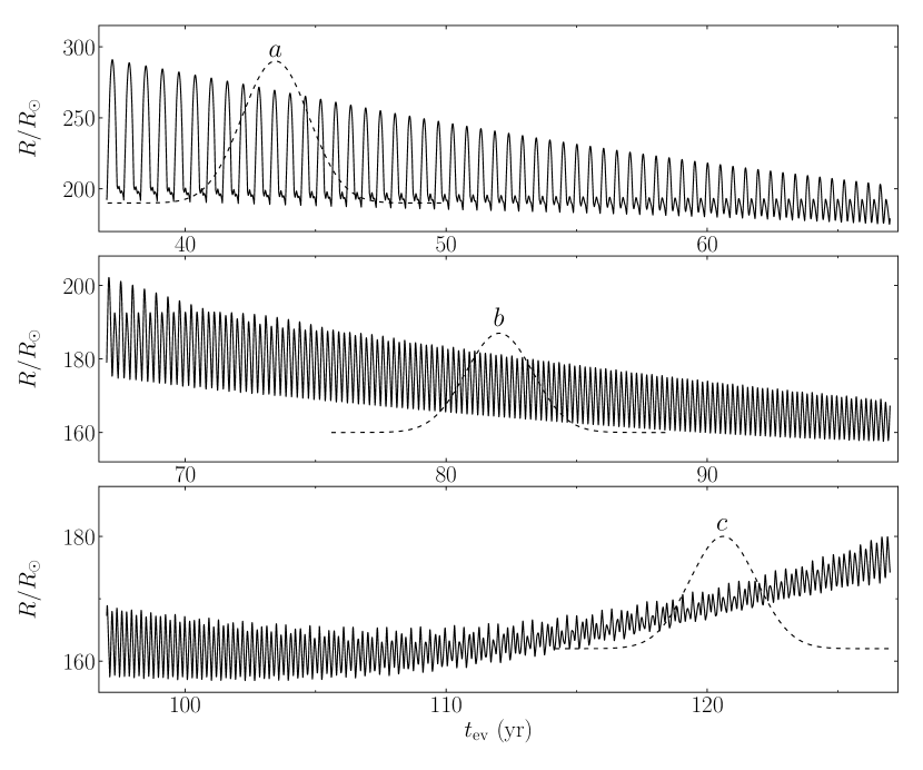
Figure 8: The radius of the outer boundary of the hydrodynamic model $M_{\mathrm{ZAMS}}=1.8M_{\sun}$, $\eta_{\mathrm{B}}=10$, $i_{\textrm{TP}}=11$ as a function of time during pulsational mode switching. Dashed lines represent the location of time intervals (gaussian windows) used for calculation of the short–time Fourier transform.

Mode switching from the fundamental mode to the first overtone is due to temperature growth in the pulsating envelope because it is accompanied by outward movement of the lower boundary of the hydrogen ionization zone in the first three decades after the peak helium–burning luminosity. Subsequent temperature decrease in the stellar envelope ($t_{\textrm{ev}}\goa 30$ yr) leads to inward movement of the lower boundary of the hydrogen ionization zone and to mode switching from the first overtone to the fundamental mode for $t_{\textrm{ev}}\goa 100$ yr.

Mode switching in the hydrodynamic model of T UMi can be also illustrated by results of the short–time Fourier transform of the temporal dependence of the stellar radius presented in Fig. 8. To this end the whole time interval of the hydrodynamic model $M_{\mathrm{ZAMS}}=1.8M_{\sun}$, $\eta_{\mathrm{B}}=10$, $i_{\textrm{TP}}=11$ ($-70~{}\textrm{yr}\leq t_{\textrm{ev}}\leq 127$ yr) was divided into 16 time intervals and the amplitude spectrum $A_{\mathrm{R}}$ was computed for the product of $R(t_{\textrm{ev}})$ and the gaussian window function $\sigma=5$ for each interval. The amplitude spectra of the stellar radius $A_{\mathrm{R}}$ are given in Fig. 9 for three intervals shown in Fig. 8 by the dashed lines. The case ’$a$’ (solid lines) corresponds to the early stage of mode switching when the amplitude of the first overtone is nearly one third of that of the fundamental mode whereas in the case ’$b$’ (dashed lines) the star became the first overtone pulsator since the spectral amplitude of the first overtone is about forty times greater in comparison with that of the fundamental mode. The amplitude spectrum shown in Fig. 9 by dotted lines (the case ’$c$’) allows us to conclude that increasing scatter of the curve $h_{1}$ in the upper panel of Fig. 5 corresponds to the beginning stage of a modal switch from the fundamental mode to the first overtone pulsation.

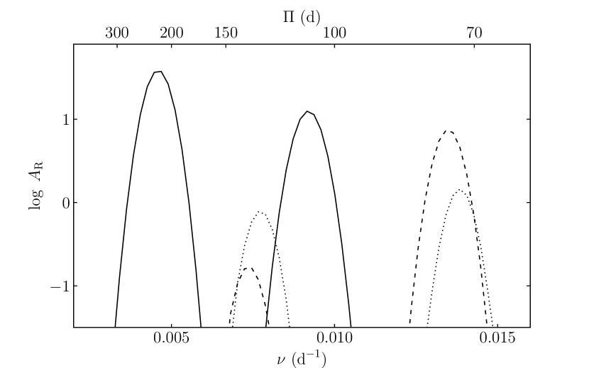
Figure 9: The amplitude spectra $A_{\mathrm{R}}$ for time intervals labelled in Fig. 8 as $a$ (solid lines), $b$ (dashed lines) and $c$ (dotted lines). The low–frequency and the high–frequency maxima of the spectra correspond to the fundamental mode and the first overtone, respectively.

Fig. 10 shows the plots of the radial displacement of Lagrangean mass zones in the hydrodynamic model $M_{\mathrm{ZAMS}}=1.8M_{\sun}$, $\eta_{\mathrm{B}}=0.1$, $i_{\textrm{TP}}=11$ for three values of the evolution time $t_{\textrm{ev}}$. For the sake of graphical representation the plots represent the normalized amplitudes $\delta r_{j}/\delta r_{N}$ because the surface amplitudes $\delta r_{N}$ significantly differ from each other. The plot for $t_{\textrm{ev}}=37$ yr corresponds to regular oscillations in the fundamental mode, whereas at the evolution time $t_{\textrm{ev}}=71$ yr the star oscillates in the first overtone. The node of the first overtone locates at the mass zone $j_{\mathrm{n}}\approx 380$ with mean radius $\langle r\rangle\approx 0.80\langle r_{N}\rangle$, whereas the inner boundary of the hydrogen ionization zone locates in mass zones $j>j_{\mathrm{n}}$. The non–zero amplitude of the radial displacement at the overtone node is due to the fact that pulsation motions are not perfectly periodic due to the presence of more than one mode. The plot for $t_{\textrm{ev}}=126$ yr corresponds to semi–regular oscillations and pulsational mode switching from the first overtone to the fundamental mode.

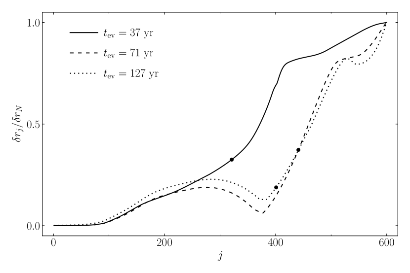
Figure 10: The normalized amplitude of the radial displacement of the $j$–th mass zone in the hydrodynamic model $M_{\mathrm{ZAMS}}=1.8M_{\sun}$, $\eta_{\mathrm{B}}=0.1$, $i_{\textrm{TP}}=11$ for $t_{\textrm{ev}}=37$ yr (solid line), $t_{\textrm{ev}}=71$ yr (dashed line) and $t_{\textrm{ev}}=115$ yr (dotted line). The mass zone $j=0$ corresponds to the inner boundary of the hydrodynamic model. Filled circles roughly indicate the inner boundary of the hydrogen ionization zone.

4 Conclusions

Calculations of non–linear stellar pulsations with time–dependent inner boundary conditions implicitly take into account effects of deviation from thermal equilibrium in the envelope of the pulsating star. As mentioned above, before the onset of period decrease ($t_{\textrm{ev}}<0$) deviation from thermal equilibrium can be neglected ($\delta_{\mathrm{L}}\loa 0.02$). However, for $t_{\textrm{ev}}>0$ deviation from thermal equilibrium rapidly increases and becomes as high as $\delta_{\mathrm{L}}\loa 0.3$ so that application of the theory of stellar pulsations with time–independent inner boundary conditions (1) leads to wrong solutions. The difference between these solutions is due to the fact that growth of the amplitude in the model computed with time–independent inner boundary conditions is accompanied by changes in the entropy structure of the pulsating star and relaxation of the model to the configuration with smaller stellar radius (Ya’Ari & Tuchman, 1996).

The hydrodynamic models of T UMi listed in Table 1 show good agreement with observational estimates of the period and the rate of period change. At the same time they are characterized by a relatively wide range of stellar masses: $1.04M_{\sun}\leq M\leq 1.48M_{\sun}$. To provide a stronger constraint on the stellar mass of T UMi one has to fix the date when the pulsation period ceases to decrease. Additional constraints on the model parameters can be obtained from observational estimates of the pulsation amplitude near the period minimum.

Data Availability

The data underlying this article will be shared on reasonable request to the corresponding author.

References

- Bloecker (1995) Bloecker T., 1995, A&A, 297, 727
- Böhm-Vitense (1958) Böhm-Vitense E., 1958, Z. Astrophys., 46, 108
- Cyburt et al. (2010) Cyburt R. H., et al., 2010, ApJS, 189, 240
- Fadeyev (2015) Fadeyev Y. A., 2015, MNRAS, 449, 1011
- Fadeyev (2018) Fadeyev Y. A., 2018, Astron. Lett., 44, 546
- Fadeyev (2021) Fadeyev Y. A., 2021, Astron. Lett., 47, 765
- Fox & Wood (1982) Fox M. W., Wood P. R., 1982, ApJ, 259, 198
- Gal & Szatmary (1995) Gal J., Szatmary K., 1995, A&A, 297, 461
- Herwig (2000) Herwig F., 2000, A&A, 360, 952
- Höfner & Olofsson (2018) Höfner S., Olofsson H., 2018, A&ARv, 26, 1
- Kuhfuss (1986) Kuhfuss R., 1986, A&A, 160, 116
- Mattei & Foster (1995) Mattei J. A., Foster G., 1995, JAAVSO, 23, 106
- Molnár et al. (2019) Molnár L., Joyce M., Kiss L. L., 2019, ApJ, 879, 62
- Paxton et al. (2019) Paxton B., et al., 2019, ApJS, 243, 10
- Pickering & Fleming (1906) Pickering E. C., Fleming W. P., 1906, ApJ, 23, 257
- Reimers (1975) Reimers D., 1975, in Baschek B., Kegel W. H., Traving G., eds, , Problems in stellar atmospheres and envelopes. Springer–Verlag, New York, pp 229–256
- Samus’ et al. (2017) Samus’ N. N., Kazarovets E. V., Durlevich O. V., Kireeva N. N., Pastukhova E. N., 2017, Astron. Rep., 61, 80
- Smelcer (2002) Smelcer L., 2002, Information Bulletin on Variable Stars, 5323, 1
- Szatmáry et al. (2003) Szatmáry K., Kiss L. L., Bebesi Z., 2003, A&A, 398, 277
- Uttenthaler et al. (2011) Uttenthaler S., et al., 2011, A&A, 531, A88
- Willson (2000) Willson L. A., 2000, ARA&A, 38, 573
- Wood & Zarro (1981) Wood P. R., Zarro D. M., 1981, ApJ, 247, 247
- Xiong & Deng (2007) Xiong D. R., Deng L., 2007, MNRAS, 378, 1270
- Ya’Ari & Tuchman (1996) Ya’Ari A., Tuchman Y., 1996, ApJ, 456, 350