Tri-Resonant Leptogenesis in a Seesaw Extension of the Standard Model

ABSTRACT

We study a class of leptogenesis models where the light neutrinos acquire their observed small masses by a symmetry-motivated construction. This class of models may naturally include three nearly degenerate heavy Majorana neutrinos that can strongly mix with one another and have mass differences comparable to their decay widths. We find that such a tri-resonant heavy neutrino system can lead to leptonic CP asymmetries which are further enhanced than those obtained in the usual bi-resonant approximation. Moreover, we solve the Boltzmann equations by paying special attention to the temperature dependence of the relativistic degrees of freedom of the plasma. The latter results in significant corrections to the evolution equations for the heavy neutrinos and the lepton asymmetry that have been previously ignored in the literature. We show the importance of these corrections to accurately describe the dynamical evolution of the baryon-to-photon ratio $\eta_{B}$ for heavy neutrino masses at and below $100~{}{\rm GeV}$, and demonstrate that successful leptogenesis at lower masses can be significantly affected by the variation of the relativistic degrees of freedom. The parameter space for the leptogenesis model is discussed, and it could be probed in future experimental facilities searching for charged lepton flavour violation and heavy neutrinos in future $Z$-boson factories.

Keywords: Seesaw; Leptogenesis; Baryon asymmetry; Boltzmann equations

1 Introduction

Observations done by the Wilkinson Microwave Anisotropy Probe (WMAP) and the Planck observatory indicate that the extent of the Baryon Asymmetry of the Universe (BAU) amounts to [1, 2]

$$\eta_{B}^{\rm CMB}=6.104\pm 0.058\times 10^{-10}.$$ (1.1)

Hence, explaining the observed BAU has been one of the central themes of Particle Cosmology for decades. The existence of this non-zero BAU is one of the greatest pieces of evidence for physics beyond the Standard Model (SM). In the SM, the neutrinos are strictly massless, and so this runs contrary to the observations of neutrino oscillations[3, 4, 5], which only exist for massive neutrinos. A minimal resolution to this problem will be to include additional heavy neutrinos which are singlets under the SM gauge group: ${\textrm{SU}(3)_{c}\times\textrm{SU}(2)_{L}\times\textrm{U}(1)_{Y}}$. These additional neutrinos are permitted to have large masses due to the inclusion of a Majorana mass term which violates lepton number, $L$, by two units. They also provide a mechanism to render the SM neutrinos massive, whilst ensuring that the generated mass is small in scale through the famous seesaw mechanism [6, 7, 8, 9]. On the other hand, the spacetime expansion of the FRW Universe provides a macroscopic arrow of cosmic time $t$, as well as Sakharov’s necessary out-of-thermal equilibrium condition [10] needed to potentially generate a large lepton-number asymmetry. This asymmetry is then rapidly converted into a baryon asymmetry through $(B+L)$-violating sphaleron transitions while the temperature of the Universe remains above the temperature $T_{\rm sph}\approx 132~{}{\rm GeV}$, after which these sphaleron transitions become exponentially suppressed. This mechanism is commonly referred to as leptogenesis [11].

A particularly interesting framework of leptogenesis is Resonant Leptogenesis (RL)[12, 13], which permits Majorana mass scales far lower than those that occur in typical Grand Unified Theory (GUT) models of leptogenesis [11, 14]. In RL models, the CP violation generated is greatly enhanced through the mixing of nearly degenerate heavy Majorana neutrinos $N_{\alpha}$, provided

$$\left|m_{N_{\alpha}}-m_{N_{\beta}}\right|\sim\frac{\Gamma_{N_{\alpha,\beta}}}{2}\;,$$

where $m_{N_{\alpha}}$ and $\Gamma_{N_{\alpha}}$ are the masses and the decay widths of $N_{\alpha}$, respectively. This mass arrangement in turn permits the generation of appreciable BAU at sub-${\rm TeV}$ masses [12, 15], in agreement with neutrino oscillation parameters [13, 16].

In this paper we study a class of leptogenesis models that may naturally include three nearly degenerate heavy Majorana neutrinos which can strongly mix with one another and have mass differences comparable to their widths. We compute the leptonic CP asymmetries generated in such a tri-resonant heavy neutrino system, to find that their size is further enhanced in comparison to those that were naively determined in the usually considered bi-resonant approximation. Accordingly, this enhanced mechanism of leptogenesis will be called Tri-Resonant Leptogenesis (TRL). In the context of models realising TRL, our aim is to find neutrino Yukawa couplings whose size lies much higher than the one expected from a typical seesaw scenario, whilst still achieving the observed BAU. To this end, we solve the Boltzmann equations (BEs) that describe the evolution of heavy neutrino and lepton-asymmetry number densities before the sphaleron freeze-out temperature, after including decay and scattering collision terms. An important novelty of the present study is to assess the significance of the temperature dependence of the relativistic degrees of freedom (dofs) in the plasma. Finally, we analyse observables of charged Lepton Flavour Violation (cLFV) that could be tested in current and projected experiments, such as ${\mu\rightarrow eee}$ at Mu3e [17], ${\mu\rightarrow e\gamma}$ at MEG  [18, 19], coherent $\mu\rightarrow e$ conversion at COMET [20] and PRISM [21], as well as matching the observed light neutrino mass constraints [3, 4, 5].

In our analysis we will not specify the origin of the structure of the Majorana-mass and the neutrino Yukawa matrices. But we envisage a high-scale SO(3)-symmetric mass spectrum for the heavy Majorana neutrinos, possibly of the order of GUT scale [22, 23], which is broken by renormalisation-group (RG) and new-physics threshold effects. Following a less constrained approach to model-building, we also assume an approximate $\mathbb{Z}_{6}$-symmetric texture for the entries of the neutrino Yukawa matrix. Such a construction enables the generation of the observed small neutrino masses, without imposing the expected seesaw suppression on the neutrino Yukawa parameters for heavy neutrino masses at the electroweak scale.

The layout of the paper is as follows. In Section 2 we describe the minimal extension of the SM that we will be studying, and introduce the flavour structure of its leptonic Yukawa sector. In Section 3 we specify the light neutrino mass spectrum for our analysis, and present the cLFV observables one may expect to probe in this model, such as ${\mu\rightarrow e\gamma}$, ${\mu\rightarrow eee}$, and coherent $\mu\to e$ conversion in nuclei. In Section 4 we explore the different aspects of leptogenesis, notably the CP violation generated in RL and TRL scenarios and derive the relevant set of BEs, upon which our numerical estimates are based. This set of BEs is solved including contributions from chemical potentials while crucially preserving the temperature dependence of the key parameter, denoted later as $h_{\rm eff}(T)$, that describes the variation of the relativistic dofs with $T$. In Section 5 we present approximate solutions to the BEs, which will help us to shed light on the attractor properties of our fully-fledged numerical estimates. In Section 6 we give a summary of our numerical results, including evolution plots for the BAU and comparisons with observable quantities. Finally, Section 7 summarises our conclusions and discusses possible future directions. Some technical aspects of our study have been relegated to Appendices A, B and C.

2 Seesaw Extension of the Standard Model

We adopt the framework of the conventional seesaw extension of the SM. This extension requires the addition of $n\geq 2$ right-handed neutrinos, which are singlets under the SM gauge group, and have lepton number $L_{\nu_{R}}=1$. Given this particle content and quantum number assignments, the Lagrangian of the right-handed neutrino sector reads:

$$\mathcal{L}_{\nu_{R}}=i\overline{\nu}_{R}\not{\partial}\nu_{R}-\left(\overline{L}\,{\bf h}^{\nu}\tilde{\Phi}\,\nu_{R}+\frac{1}{2}\overline{\nu}^{C}_{R}\,{\bf m}_{M}\nu_{R}+{\rm H.c.\,}\right).$$ (2.1)

Here, $L_{i}=(\nu_{iL},e_{iL})^{\sf T}$, with $i=1,2,3$, denote the left-handed lepton doublets, while $\nu_{\alpha R}$, with $\alpha=1,...,n$, are the right-handed neutrino fields. The matrices ${\bf h}^{\nu}$ and ${\bf m}_{M}$ are the neutrino Yukawa and the Majorana mass matrices, respectively, and $\tilde{\Phi}$ is the weak isospin conjugate of the Higgs doublet $\Phi$. Note that we reserve bold face for matrices in flavour space, and assume the implicit contraction of flavour space indices.

Without loss of generality, we assume that the Majorana mass matrix is diagonal, in which case we may recast the Lagrangian (2.1) in the unbroken phase as

$$\mathcal{L}_{\nu_{R}}=i\overline{N}\not{\partial}N-\left(\overline{L}\,{\bf h}^{\nu}\tilde{\Phi}\,P_{R}N+{\rm H.c.}\right)-\frac{1}{2}\overline{N}\,{\bf m}_{M}N,$$ (2.2)

where $P_{R/L}=\frac{1}{2}\left({\bf 1}_{4}\pm\gamma_{5}\right)$ is the right-/left- chiral projector, ${\bf 1}_{n}$ is the $n\times n$ identity matrix, ${\bf m}_{M}={\rm diag}(m_{N_{1}},...,m_{N_{n}})$, and $N_{\alpha}=\nu_{\alpha R}+\nu^{C}_{\alpha R}$ are the mass-eigenstate Majorana spinors associated to the right-handed neutrinos.

In the broken phase, this picture changes by the mixing between singlet and left-handed neutrinos. The mass eigenstates are particular combinations of the weak eigenstate neutrinos, given by

$$P_{R}\begin{pmatrix}\nu\\ N\end{pmatrix}=\begin{pmatrix}U_{\nu\nu_{L}^{C}}&U_{\nu\nu_{R}}\\ U_{N\nu_{L}^{C}}&U_{N\nu_{R}}\end{pmatrix}\begin{pmatrix}\nu_{L}^{C}\\ \nu_{R}\end{pmatrix}\;,$$ (2.3)

where $\nu_{1,2,3}$ are the light neutrino mass eigenstates and $U$ is a $(3+n)\times(3+n)$ unitary matrix that diagonalises the neutrino mass matrix (see Section 2.1). The subscripts, $\nu^{C}_{L}$ and $\nu_{R}$, on its sub-blocks indicate the possible components of the right-handed chirality projection of each mass eigenstate, represented here as vector columns $\nu$ and $N$. Following the notation of [24], we may then write the Lagrangian for the charged current interaction of the heavy neutrinos as

$$\mathcal{L}^{W}_{\rm int}=-\frac{g_{w}}{\sqrt{2}}W^{-}_{\mu}\overline{e}_{iL}B_{i\alpha}\gamma^{\mu}P_{L}N_{\alpha}+{\rm H.c.}\,,$$ (2.4)

where $g_{w}$ is the gauge coupling associated to the SU(2)_L group, and

$$B_{i\alpha}\simeq\xi_{i\alpha}=({\bf m}_{D}{\bf m}^{-1}_{M})_{i\alpha}$$ (2.5)

is the light-to-heavy neutrino mixing at first order in the expansion of the matrix-valued parameter $\xi$ [24]. In the following, we assume that the charged lepton Yukawa matrix is diagonal, and hence $B_{i\alpha}=(U_{\nu\nu_{R}})_{i\alpha}$. At first order in $\xi$, the effective light neutrino mass matrix, ${\bf m}^{\nu}$, follows the well-known seesaw relation [7]

$${\bf m}^{\nu}=-{\bf m}_{D}{\bf m}^{-1}_{M}{\bf m}^{\sf T}_{D}\;,$$ (2.6)

where ${\bf m}_{D}={\bf h}^{\nu}v/\sqrt{2}$ is the Dirac mass matrix, and $v\simeq 246~{}{\rm GeV}$ is the vacuum expectation value (VEV) of the Higgs field. By virtue of this relation, it is apparent that a Dirac mass matrix at a scale

$$|\!|{\bf m}_{D}|\!|\equiv\sqrt{\textrm{Tr}\left[\mathbf{m}_{D}^{\dagger}\mathbf{m}_{D}\right]}\approx v\;,$$ (2.7)

would in principle require GUT scale heavy neutrinos, which means that any impact of the singlet neutrino sector on experimental signatures would be beyond the realm of observation. This motivates the search for new model building strategies to explain sub-${\rm eV}$ light neutrinos, whilst maintaining agreement with light neutrino data and other low energy experiments.

2.1 Neutrino Flavour Model

In order to explain the smallness of neutrino masses, we investigate scenarios where the neutrino mass matrix is naturally small, preferably arising from the subtle breaking of a symmetry. When this symmetry is exact, (2.6) vanishes identically, given by the $3\times 3$ null matrix, $\mathbf{0}_{3}$, i.e.

$${\bf m}_{D}\,{\bf m}^{-1}_{M}\,{\bf m}^{\sf T}_{D}\,=\,{\bf 0}_{3}\;.$$ (2.8)

If we consider a singlet neutrino sector with a nearly degenerate mass spectrum, this is approximately equivalent to require that prior to the breaking of the symmetry the leading Yukawa matrix, ${\bf h}^{\nu}_{0}$, satisfies the condition

$${\bf h}^{\nu}_{0}\,{\bf h}^{\nu\sf T}_{0}\,=\,{\bf 0}_{3}\;.$$ (2.9)

Considering a model with three right-handed neutrinos, this motivates the following structure for the leading neutrino Yukawa matrix:

$${\bf h}^{\nu}_{0}=\begin{pmatrix}a&a\,\omega&a\,\omega^{2}\\ b&b\,\omega&b\,\omega^{2}\\ c&c\,\omega&c\,\omega^{2}\end{pmatrix}\;,$$ (2.10)

where the parameters $a$, $b$, and $c$ are in general real, and $\omega$ is the generator of the $\mathbb{Z}_{6}$ group, $\omega=\exp(\pi i/3)$. We remark that this choice is not unique, and the vanishing of the light neutrino mass matrix may be realised through other constructions of the neutrino Yukawa matrix. For example, one could replace the $\mathbb{Z}_{6}$ element $\omega$ with the $\mathbb{Z}_{3}$ element $\omega^{\prime}=\exp(-2\pi i/3)$. However, for concreteness, we select the $\mathbb{Z}_{6}$-symmetry realisation for our analysis.

Evidently, the flavour structure of (2.10) has to be perturbed in order to reproduce the observed neutrino oscillation phenomenon, which requires massive neutrinos. Even though ${\bf h}^{\nu}_{0}$ as given by (2.10) is rank one, a perturbation $\delta{\bf h}^{\nu}$ such that rank($\delta{\bf h}^{\nu})\geq 2$ is sufficient to explain neutrino oscillations, as long as the following condition is enforced:

$$({\bf h}^{\nu}_{0}+\delta{\bf h}^{\nu})\,{\bf m}_{M}^{-1}\,({\bf h}^{\nu}_{0}+\delta{\bf h}^{\nu})^{\sf T}\,=\,\frac{2}{v^{2}}\,{\bf m}^{\nu}\;.$$ (2.11)

where ${\bf m}^{\nu}$ is a $3\times 3$ complex and symmetric matrix. Taking $a$, $b$, $c$, and the singlet neutrino spectrum as input parameters, (2.11) defines a set of $12$ constraints for the entries of the perturbation matrix $\delta{\bf h}^{\nu}$. The solutions to (2.11) have to satisfy a further condition, which is $|\delta{\bf h}^{\nu}_{ij}|/|({\bf h}^{\nu}_{0})_{kl}|\ll 1$, with $i,j,k,l=1,2,3$. More generally, the zero mass condition of (2.9) can be enforced when the Majorana mass matrix ${\bf m}_{M}$ is not proportional to the identity, or even in the case when loop corrections to the tree-level seesaw relation of (2.6) are considered. This gives us complete control over the loop corrections to the light-neutrino mass matrix at all orders. For example, we can incorporate one-loop corrections to $\mathbf{m}^{\nu}$ [24] by modifying the tree-level zero mass condition as follows [25]:

$${\bf h}^{\nu}_{0}\left[{\bf m}^{-1}_{M}-\frac{\alpha_{w}}{16\pi M^{2}_{W}}{\bf m}^{\dagger}_{M}f({\bf m}_{M}{\bf m}^{\dagger}_{M})\right]{\bf h}^{\nu\sf T}_{0}=\,\mathbf{0}_{3}\;,$$ (2.12)

where

$$f({\bf m}_{M}{\bf m}^{\dagger}_{M})=\frac{M^{2}_{H}}{{\bf m}_{M}{\bf m}^{\dagger}_{M}-M^{2}_{H}{\bf 1}_{3}}\ln\left(\frac{{\bf m}_{M}{\bf m}^{\dagger}_{M}}{M^{2}_{H}}\right)+\frac{3M^{2}_{Z}}{{\bf m}_{M}{\bf m}^{\dagger}_{M}-M^{2}_{Z}{\bf 1}_{3}}\ln\left(\frac{{\bf m}_{M}{\bf m}^{\dagger}_{M}}{M^{2}_{Z}}\right)\;.$$ (2.13)

In the above, $\alpha_{w}\equiv g_{w}^{2}/(4\pi)^{2}$ is the electroweak-coupling parameter, and $M_{W}$, $M_{Z}$, and $M_{H}$ are the masses of the $W$, $Z$, and Higgs bosons, respectively. Redefining the quantity inside the square brackets in (2.12) as an effective inverse Majorana mass, $\overline{{\bf m}}_{M}^{-1}$, the restrictions can be recast as

$${\bf h}^{\nu}_{0}\overline{{\bf m}}_{M}^{-1}{\bf h}^{\nu\sf T}_{0}=\,\mathbf{0}_{3}\;.$$ (2.14)

This can be further simplified by rescaling the columns of the Yukawa matrix using the definition

$${\bf H}^{\nu}_{0}={\bf h}^{\nu}_{0}\,\overline{{\bf m}}^{-1/2}_{M}\;,$$ (2.15)

which leads to

$${\bf H}^{\nu}_{0}\,{{\bf H}^{\nu}_{0}}^{\sf T}=\,\mathbf{0}_{3}\;.$$ (2.16)

This results in the same condition of (2.9) but this time for a rescaled Yukawa matrix, ${\bf H}^{\nu}_{0}$, with dimensions of (mass)^-1/2. This shows that even for appreciable mass splittings between the singlet neutrinos and with the inclusion of loop corrections to the neutrino mass matrix, the Yukawa matrix can always be chosen in such a way that the neutrinos are massless by taking

$${\bf H}^{\nu}_{0}=\begin{pmatrix}\ell_{1}&\ell_{1}\,\omega&\ell_{1}\,\omega^{2}\\ \ell_{2}&\ell_{2}\,\omega&\ell_{2}\,\omega^{2}\\ \ell_{3}&\ell_{3}\,\omega&\ell_{3}\,\omega^{2}\end{pmatrix}\;,$$ (2.17)

where $\ell_{1,2,3}$ are real parameters. The dimensionless Yukawa matrix, ${\bf h}^{\nu}_{0}$, can be found using (2.15), and as explained previously, its structure can then be perturbed to reproduce the observed neutrino mass matrix ${\bf m}^{\nu}$. Here we will not address the origin of the texture of the neutrino Yukawa matrix ${\bf h}^{\nu}_{0}$, but it can be the subject of future studies on model building.

It is worthy to mention that the neutrino mass matrix is model dependent, and its relation to the observable parameters measured in neutrino oscillation experiments is given by

$${\bf m}^{\nu}=U_{\textrm{PMNS}}^{\sf T}\,\widehat{{\bf m}}^{\nu}U_{\textrm{PMNS}}\;,$$ (2.18)

where $U_{\textrm{PMNS}}$ is the PMNS lepton mixing matrix [26, 27] and $\widehat{{\bf m}}^{\nu}={\rm diag}(m_{1},m_{2},m_{3})$, in which $m_{1,2,3}$ are the light neutrino masses. The matrix $U_{\textrm{PMNS}}$ performs the Takagi factorisation [28, 29] when applied to the light neutrino mass matrix. If the Yukawa matrix of the charged leptons is assumed to be diagonal, $U_{\textrm{PMNS}}$ parameterises the flavour mixing in charged current interactions of the leptonic sector. The experimental values of the parameters involved in (2.18) are discussed in the next section.

3 Low Energy Observables

The observation of flavour neutrino oscillations at Super-Kamiokande [5] and the Sudbury Neutrino Observatory [3, 4] provides definite evidence of their massive nature. The resulting neutrino oscillation parameters offer strong constraints on the neutrino model parameters, which we discuss in this section. In addition, we present the formulae for the rates of selected charged cLFV processes, namely $\mu\rightarrow e\gamma$, $\mu\rightarrow eee$ and coherent $\mu\rightarrow e$ conversion in nuclei, which can be distinctive signatures of Majorana neutrino models, and are crucially dependent on the light-to-heavy neutrino mixing parameter presented in (2.5).

3.1 Neutrino Oscillation Data

In order to incorporate the neutrino mass constraints into our model, we follow the procedure outlined in Section 2.1. We neglect the non-unitarity effects that arise due to light-to-heavy neutrino mixing, and without loss of generality, we assume that the charged lepton Yukawa matrix, ${\bf h}^{\ell}$, is diagonal. With the first assumption in mind, the matrix $U_{\textrm{PMNS}}$ can be parameterised as follows [30, 31]:

$$U_{\textrm{PMNS}}\ =\ \begin{pmatrix}c_{12}c_{13}&s_{12}c_{13}&s_{13}e^{-i\delta}\\ -s_{12}c_{23}-c_{12}s_{23}s_{13}e^{i\delta}&c_{12}c_{23}-s_{12}s_{23}s_{13}e^{i\delta}&s_{23}c_{13}\\ s_{12}c_{23}-c_{12}c_{23}s_{13}e^{i\delta}&-c_{12}s_{23}-s_{12}c_{23}s_{13}e^{i\delta}&c_{23}c_{13}\end{pmatrix}\times\text{diag}(e^{i\alpha_{1}/2},e^{i\alpha_{2}/2},1)\;,$$ (3.1)

where $c_{ij}=\cos\theta_{ij}$ and $s_{ij}=\sin\theta_{ij}$ are the cosines and sines of the neutrino mixing angles, $\delta$ is the so-called Dirac phase, and $\alpha_{1,2}$ are the Majorana phases. Together with the neutrino squared mass differences $\Delta m^{2}_{21}\equiv m^{2}_{2}-m^{2}_{1}$ and $\Delta m^{2}_{31}\equiv m^{2}_{3}-m^{2}_{1}$, these angles and the Dirac phase comprise the light neutrino oscillation data.

The values of these parameters are experimentally bounded with the exception of the absolute neutrino mass scale, characterised by min($m_{1,3}$), and the sign of $\Delta m^{2}_{31}\equiv m^{2}_{3}-m^{2}_{1}$, which requires the distinction between the normal ($\Delta m^{2}_{31}>0$) and inverted ($\Delta m^{2}_{31}<0$) ordering hypotheses. For our numerical estimates, we use the latest best fit values for the neutrino oscillation parameters [32]:

$$\Delta m^{2}_{21}\equiv m^{2}_{2}-m^{2}_{1}=7.50\times 10^{-5}\,(\text{eV})^{2},\quad\Delta m^{2}_{31}\equiv m^{2}_{3}-m^{2}_{1}=2.55\times 10^{-3}\,(\text{eV})^{2},$$ (3.2)

$$\theta_{12}=34.3^{\circ},\quad\theta_{23}=49.26^{\circ},\quad\theta_{13}=8.58^{\circ},\quad\delta=194^{\circ}.$$ (3.3)

Since the experimental data allows a massless neutrino, for definiteness we work under the hypothesis that $m_{1}=0$ and the light neutrino spectrum follows normal ordering. Likewise, for the unconstrained Majorana phases, we set $\alpha_{1,2}=0$. For relevant tri-resonant benchmarks, we provide the relevant $\delta{\bf h}^{\nu}$ values, which reproduce the light neutrino data in Appendix C.

3.2 Lepton Flavour Violation

In the seesaw extension of the SM, the leading order contributions to cLFV processes appear at the one-loop level [33]. For the radiative decays of our interest, the expressions for the branching ratios are given by [34]

$${\rm BR}(\mu\to e\gamma) =\frac{\alpha_{w}^{3}s_{w}^{2}}{256\pi^{2}}\frac{m_{\mu}^{4}}{M_{W}^{4}}\>\frac{m_{\mu}}{\Gamma_{\mu}}\left|G_{\gamma}^{\mu e}\right|^{2},$$ (3.4)

$${\rm BR}(\mu\to eee) =\frac{\alpha_{w}^{4}}{24576\pi^{3}}\>\frac{m_{\mu}^{4}}{M_{W}^{4}}\frac{m_{\mu}}{\Gamma_{\mu}}\left\{2\left|\frac{1}{2}F_{\rm Box}^{\mu eee}+F_{Z}^{\mu e}-2s_{w}^{2}\left(F_{Z}^{\mu e}-F_{\gamma}^{\mu e}\right)\right|^{2}\right.$$

$$\left.+\ 4s_{w}^{4}\left|F_{Z}^{\mu e}-F_{\gamma}^{\mu e}\right|^{2}+16s_{w}^{2}\,\Re e\left[\left(F_{Z}^{\mu e}+\frac{1}{2}F_{\rm Box}^{\mu eee}\right)G_{\gamma}^{\mu e*}\right]\right.$$ (3.5)

$$\left.-\ 48s_{w}^{4}\,\Re e\,\left[\left(F_{Z}^{\mu e}-F_{\gamma}^{\mu e}\right)G_{\gamma}^{\mu e*}\right]+32s_{w}^{4}\left|G_{\gamma}^{\mu e}\right|^{2}\left[\ln\left(\frac{m_{\mu}^{2}}{m^{2}_{e}}\right)-\frac{11}{4}\right]\right\}\;,$$

where $s_{w}\equiv\sin\theta_{w}$ is the sine of the weak angle, $m_{e}$ is the mass of the electron, and $m_{\mu}$ and $\Gamma_{\mu}$ are the muon mass and width. The form factors are defined in Appendix B. It is worth mentioning that other cLFV decays involving $\tau$ leptons are also allowed, but we ignore them in the discussion of our results since the experimental bounds that apply to those processes are far weaker in the parameter space of interest to us.

The rate for the $\mu\to e$ conversion in an atomic nucleus ${}_{Z}^{A}X$ is given by [35]

$$R^{X}_{\mu\to e}\ =\ \frac{2G_{F}^{2}\alpha_{w}^{2}m_{\mu}^{5}}{16\pi^{2}\Gamma_{\rm capt}}\ \left|4V^{(p)}\left(2\tilde{F}_{u}^{\mu e}+\tilde{F}_{d}^{\mu e}\right)+4V^{(n)}\left(\tilde{F}_{u}^{\mu e}+2\tilde{F}_{d}^{\mu e}\right)+\frac{s_{w}^{2}}{2e}G_{\gamma}^{\mu e}D\right|^{2}\;,$$ (3.6)

where $G_{F}$ is Fermi’s constant, $e=g_{w}s_{w}$ is charge of the electron, $\Gamma_{\rm capt}$ is the nuclear capture rate, and $V^{(p)},V^{(n)},D$ are numerical estimations of the overlap integrals involved in the calculation of the conversion rate [36]. For the nuclei of our interest, Table 1 presents the numerical values of these parameters. The form factors $\tilde{F}_{q}^{\mu e}$ $(q=u,d)$ in (3.6) are defined as

$$\tilde{F}_{q}^{\mu e}\ =\ Q_{q}s_{w}^{2}F_{\gamma}^{\mu e}\;+\;\left(\frac{I^{q}_{3}}{2}-Q_{q}s_{w}^{2}\right)F_{Z}^{\mu e}\;+\;\frac{1}{4}F_{\rm Box}^{\mu eqq}\;,$$ (3.7)

where $Q_{u}=2/3$, $Q_{d}=-1/3$ refer to the electric charges of up- and down-type quarks, and $I^{u}_{3}=1/2$, $I^{d}_{3}=-1/2$ denote the third component of their weak isospin. The corresponding form factors can be found in Appendix B.

Nucleus (${}_{Z}^{A}X$)	$V^{(p)}$	$V^{(n)}$	$D$	$\Gamma_{\rm capt}~{}(10^{6}~{}{\rm s}^{-1})$
${}_{13}^{27}$Al	0.0161	0.0173	0.0362	13.45
${}_{22}^{48}$Ti	0.0396	0.0468	0.0864	2.59
${}_{79}^{197}$Au	0.0974	0.146	0.189	13.07

Table 1: Overlap integrals and muon capture rates for the nuclei of the elements used in the relevant experiments.

The search for cLFV is a prominent experimental endeavour, and there are several facilities that operate with the aim of finding a conclusive hint for this class of transitions. Despite the non-observation of these signals, experimental efforts have lead to stringent bounds on the parameter space of Majorana neutrino models, which are reflected by the current upper limits

$${\rm BR}(\mu\rightarrow e\gamma) <4.2\times 10^{-13}\qquad\text{MEG~{}\cite[cite]{[\@@bibref{}{MEG:2016leq}{}{}]}}\;,$$

$${\rm BR}(\mu\rightarrow eee) <1.0\times 10^{-12}\qquad\text{SINDRUM~{}\cite[cite]{[\@@bibref{}{SINDRUM:1987nra}{}{}]}}\;,$$ (3.8)

$$R^{\rm Au}_{\mu\rightarrow e} <7.0\times 10^{-13}\qquad\text{SINDRUM~{}\cite[cite]{[\@@bibref{}{SINDRUMII:2006dvw}{}{}]}}\;.$$

These limits are expected to be improved by a few orders of magnitude in the near future. There is a new generation of experiments that are either starting to take data, under construction, or in the proposal/design stage. Among them, we should mention MEG-II, COMET, Mu3e, Mu2e and PRISM, with the following projected sensitivities:

$${\rm BR}(\mu\rightarrow e\gamma) <6\times 10^{-14}\qquad\text{MEG II~{}\cite[cite]{[\@@bibref{}{MEGII:2018kmf}{}{}]}},$$

$${\rm BR}(\mu\rightarrow eee) <10^{-16}\qquad\text{\quad\,\, Mu3e~{}\cite[cite]{[\@@bibref{}{Blondel:2013ia}{}{}]}},$$

$$R^{\rm Al}_{\mu\rightarrow e} <3\times 10^{-17}\qquad\text{Mu2e~{}\cite[cite]{[\@@bibref{}{DiFalco:2022kqz}{}{}]}},$$ (3.9)

$$R^{\rm Al}_{\mu\rightarrow e} <10^{-17}\;\,\,\quad\qquad\text{COMET~{}\cite[cite]{[\@@bibref{}{Moritsu:2022lem}{}{}]}},$$

$$R^{\rm Ti}_{\mu\rightarrow e} <10^{-18}\qquad\text{\quad\,\, PRISM~{}\cite[cite]{[\@@bibref{}{BARLOW201144}{}{}]}}.$$

These projections will be compared with the cLFV rates as predicted by our leptogenesis model to assess its testability in the foreseeable future.

3.2.1 Non-Zero Leptonic CP Phases in cLFV Processes

Here we examine the impact of leptonic CP phases on cLFV processes for our class of seesaw models. It was argued in [40] that the existence of non-zero leptonic CP phases may have a substantive impact on the rate of cLFV processes through the interference terms involving the mixing $B_{\ell\alpha}$. Following a procedure similar to [40], we write the elements of $B_{i\alpha}$ as a magnitude $s_{i\alpha}$ and a phase $\varepsilon_{i\alpha}$. Thus, the terms that appear in the observable quantities are

$$\sum_{\alpha=1}^{3}B_{i\alpha}B_{j\alpha}^{*}=\sum_{\alpha=1}^{3}s_{i\alpha}s_{j\alpha}e^{i(\varepsilon_{i\alpha}-\varepsilon_{j\alpha})}=\sum_{\alpha=1}^{3}s_{i\alpha}s_{j\alpha}e^{i\Delta^{ij}_{\alpha}}\;,$$ (3.10)

where we have introduced the CP phases $\Delta^{ij}_{\alpha}=\varepsilon_{i\alpha}-\varepsilon_{j\alpha}$. These CP phases are expected to be small and can easily be extracted by taking the ratio of imaginary to real parts of the mixing, i.e.

$$\frac{\Im m\left\{B_{i\alpha}B_{j\alpha}^{*}\right\}}{\Re e\left\{B_{i\alpha}B_{j\alpha}^{*}\right\}}=\tan\left(\Delta_{\alpha}^{ij}\right)\approx\Delta_{\alpha}^{ij}\;.$$ (3.11)

For the model introduced in Section 2, the heavy neutrino masses are nearly degenerate and the elements of the mixing matrix are all of similar scale. Therefore, the observable quantities may be approximated by taking the masses to be exactly degenerate and letting ${s_{i\alpha}\approx s_{i1}}$ for all $\alpha$. Under these simplifications, the variations in the cLFV observables are captured in the value of

$$\left|\sum_{\alpha=1}^{3}B_{i\alpha}B_{j\alpha}^{*}\right|^{2}\approx s_{i1}^{2}s_{j1}^{2}\sum_{\alpha,\beta=1}^{3}\cos\left(\Delta_{\alpha}^{ij}-\Delta_{\beta}^{ij}\right)\;.$$ (3.12)

Then, the observed deviation due to the existence of non-zero leptonic CP phases may be written as

$$D^{ij}=1-\frac{\left|\sum_{\alpha=1}^{3}B_{i\alpha}B_{j\alpha}^{*}\right|^{2}}{\left|\sum_{\alpha=1}^{3}B_{i\alpha}B_{j\alpha}^{*}\right|^{2}_{\Delta_{i}=0}}\approx 1-\frac{1}{9}\sum_{\alpha,\beta=1}^{3}\cos\left(\Delta_{\alpha}^{ij}-\Delta_{\beta}^{ij}\right)\;.$$ (3.13)

In the case of small leptonic CP phases, it can be seen that the deviation in the rate of cLFV processes away from the CP conserving rate may be given by

$$D^{ij}\approx\frac{1}{9}\left[\left(\Delta_{1}^{ij}-\Delta_{2}^{ij}\right)^{2}+\left(\Delta_{1}^{ij}-\Delta_{3}^{ij}\right)^{2}+\left(\Delta_{2}^{ij}-\Delta_{3}^{ij}\right)^{2}\right],$$ (3.14)

and so the observed deviation is itself a small effect.

In the context of the $\mathbb{Z}_{6}$ motivated model we have presented, the quantity $B_{i\alpha}B_{j\alpha}^{*}$ is completely real at lowest order, and therefore the leptonic CP phases are identically zero. Therefore, in order to have non-zero leptonic CP phases, we need to include the symmetry breaking term $\delta\mathbf{h}^{\nu}$. It is then not easy to verify that up to leading order in the perturbations, $\delta\mathbf{h}^{\nu}$, the relevant leptonic CP phases are given by

$$\Delta^{ij}_{\alpha}\approx\frac{\Im m\left\{(\mathbf{h}^{\nu}_{0}\mathbf{m}_{M}^{-1})_{i\alpha}(\delta\mathbf{h}^{\nu}\mathbf{m}_{M}^{-1})_{j\alpha}^{*}+(\delta\mathbf{h}^{\nu}\mathbf{m}_{M}^{-1})_{i\alpha}(\mathbf{h}^{\nu}_{0}\mathbf{m}_{M}^{-1})_{j\alpha}^{*}\right\}}{(\mathbf{h}^{\nu}_{0}\mathbf{m}_{M}^{-1})_{i\alpha}(\mathbf{h}^{\nu}_{0}\mathbf{m}_{M}^{-1})_{j\alpha}^{*}}\;.$$ (3.15)

Hence, $|\Delta_{\alpha}^{ij}|\sim|\!|\delta\mathbf{h}^{\nu}|\!|/|\!|\mathbf{h}^{\nu}_{0}|\!|\ll 1$. We may therefore expect the deviation away from the CP conserving cLFV observables to be very small in magnitude, $D^{ij}\sim|\!|\delta\mathbf{h}^{\nu}|\!|^{2}/(9|\!|\mathbf{h}^{\nu}_{0}|\!|^{2})$ . For the generic scenarios listed in Appendix C, one finds a deviation of $D^{ij}\sim 10^{-3}$, so any CP effect will be difficult to observe for the TRL models under study.

4 Tri-Resonant Leptogenesis

4.1 Leptonic Asymmetries

In leptogenesis, the CP violating effects that lead to the generation of a net baryon asymmetry come from the difference between the decay rate of heavy neutrinos into Higgs and leptons, and their charge-conjugate processes. In RL models, the absorptive part of the wavefunction contribution to the decay rate [41] is central to capture the resonance effects that arise in models with nearly degenerate singlet neutrino masses, and that result in the enhancement of CP violation [42]. To facilitate the presentation of the analytic results for the CP asymmetry in heavy neutrino decays within this framework, we introduce the coefficients [13, 16]

$$A_{\alpha\beta} =\sum_{l=1}^{3}\frac{{\bf h}^{\nu}_{l\alpha}{\bf h}_{l\beta}^{\nu*}}{16\pi}=\frac{({\bf h}^{\nu\dagger}{\bf h}^{\nu})^{*}_{\alpha\beta}}{16\pi},$$ (4.1)

$$V_{l\alpha} =\sum_{k=1}^{3}\sum_{\gamma\neq\alpha}\frac{{\bf h}^{\nu*}_{k\alpha}{\bf h}^{\nu}_{k\gamma}{\bf h}^{\nu}_{l\gamma}}{16\pi}f\left(\frac{m^{2}_{N_{\gamma}}}{m^{2}_{N_{\alpha}}}\right),$$ (4.2)

which pertain to the absorptive transition amplitudes for the propagator and vertex, respectively. Here ${f(x)=\sqrt{x}\left[1-(1+x)\ln\left(\frac{1+x}{x}\right)\right]}$ is the Fukugita-Yanagida one-loop function [11].

A full and consistent resummation of the CP-violating loop corrections, including three Majorana neutrino mixing, generates the following effective $L\tilde{\Phi}N$ Yukawa couplings [13, 16, 22]:

$$(\bar{\mathbf{h}}^{\nu}_{+})_{l\alpha}= \;{\bf h}^{\nu}_{l\alpha}+iV_{l\alpha}-i\sum_{\beta,\gamma=1}^{3}|\varepsilon_{\alpha\beta\gamma}|\,{\bf h}^{\nu}_{l\beta}$$

$$\times\frac{m_{N_{\alpha}}\left(M_{\alpha\alpha\beta}+M_{\beta\beta\alpha}\right)-iR_{\alpha\gamma}\left[M_{\alpha\gamma\beta}\left(M_{\alpha\alpha\gamma}+M_{\gamma\gamma\alpha}\right)+M_{\beta\beta\gamma}\left(M_{\alpha\gamma\alpha}+M_{\gamma\alpha\gamma}\right)\right]}{m_{N_{\alpha}}^{2}-m_{N_{\beta}}^{2}+2im^{2}_{N_{\alpha}}A_{\beta\beta}+2i\,\Im mR_{\alpha\gamma}\left(m_{N_{\alpha}}^{2}|A_{\beta\gamma}|^{2}+m_{N_{\beta}}m_{N_{\gamma}}\Re eA_{\beta\gamma}^{2}\right)}\;,$$ (4.3)

where $\epsilon_{\alpha\beta\gamma}$ is the anti-symmetric Levi-Civita symbol, $M_{\alpha\beta\gamma}\equiv m_{N_{\alpha}}A_{\beta\gamma}$ and

$$R_{\alpha\beta}\equiv\frac{m_{N_{\alpha}}^{2}}{m_{N_{\alpha}}^{2}-m_{N_{\beta}}^{2}+2im_{N_{\alpha}}^{2}A_{\beta\beta}}\;.$$ (4.4)

The corresponding CP-conjugate effective Yukawa coupling, which is associated to the $L^{C}\tilde{\Phi}^{*}N$ interaction, is denoted by $(\bar{\mathbf{h}}^{\nu}_{-})_{l\alpha}$, and it can be found through the replacement of ${\bf h}^{\nu}_{l\alpha}$ with $({\bf h}^{\nu}_{l\alpha})^{*}$ in (4.1). Notably, this resummed Yukawa coupling captures all possible degrees of resonance between the contributions to the CP asymmetry from the mixing between the singlet neutrinos, which includes the bi-resonant and tri-resonant cases. We should clarify here that the bi-resonant case implies maximally enhanced CP asymmetries through the mixing of two singlet neutrinos, and the tri-resonant implies maximally enhanced CP asymmetries through the mixing of all three singlet neutrinos. Moreover, in this formalism CP violation comes from the difference between the resummed Yukawa couplings $(\bar{\mathbf{h}}^{\nu}_{-})_{l\alpha}$ and $(\bar{\mathbf{h}}^{\nu}_{+})_{l\alpha}$, as it can be seen by calculating the heavy neutrino decay rates and scattering amplitudes with the help of (4.1). Note that for a model with two right-handed neutrinos (or equivalently, for a model utilising the bi-resonant approximation), the resummed Yukawa matrices are found by setting $R_{\alpha\beta}$ to zero in (4.1).

Using these effective Yukawa couplings, the partial decay widths of the heavy neutrinos read

$$\Gamma(N_{\alpha}\rightarrow L_{l}\Phi)=\frac{m_{N_{\alpha}}}{8\pi}\left|(\bar{{\bf h}}^{\nu}_{+})_{l\alpha}\right|^{2},\qquad\Gamma(N_{\alpha}\rightarrow L^{C}_{l}\Phi^{\dagger})=\frac{m_{N_{\alpha}}}{8\pi}\left|(\bar{\mathbf{h}}^{\nu}_{-})_{l\alpha}\right|^{2}\;.$$ (4.5)

In turn, these decay rates can be used to find the size of the CP asymmetries for each lepton family, which for a given right-handed neutrino $N_{\alpha}$ are defined as

$$\delta_{\alpha l}\equiv\frac{\Gamma(N_{\alpha}\rightarrow L_{l}\Phi)-\Gamma(N_{\alpha}\rightarrow L^{C}_{l}\Phi^{\dagger})}{\sum_{k=e,\mu,\tau}\Gamma(N_{\alpha}\rightarrow L_{k}\Phi)+\Gamma(N_{\alpha}\rightarrow L^{C}_{k}\Phi^{\dagger})}=\frac{\left|(\bar{\mathbf{h}}^{\nu}_{+})_{l\alpha}\right|^{2}-\left|(\bar{\mathbf{h}}^{\nu}_{-})_{l\alpha}\right|^{2}}{(\bar{\mathbf{h}}^{\nu\dagger}_{+}\bar{\mathbf{h}}^{\nu}_{+})_{\alpha\alpha}+(\bar{\mathbf{h}}^{\nu\dagger}_{-}\bar{\mathbf{h}}^{\nu}_{-})_{\alpha\alpha}}.$$ (4.6)

We also define the total CP asymmetry, $\delta_{\alpha}$, associated with each heavy neutrino species:

$$\delta_{\alpha}\equiv\sum_{l=e,\mu,\tau}\delta_{\alpha l}\;.$$ (4.7)

In particular, a non-vanishing $\delta_{\alpha}$ may only be generated in models, for which the flavour- and rephasing-invariant CP-odd quantity

$$\Delta_{CP} =\Im m\left\{\textrm{Tr}\left[(\mathbf{h}^{\nu})^{\dagger}\mathbf{h}^{\nu}\mathbf{m}_{M}^{\dagger}\mathbf{m}_{M}\mathbf{m}_{M}^{\dagger}(\mathbf{h}^{\nu})^{\sf T}(\mathbf{h}^{\nu})^{*}\mathbf{m}_{M}\right]\right\}$$ (4.8)

$$=\sum_{\alpha<\beta}m_{N_{\alpha}}m_{N_{\beta}}\left(m_{N_{\alpha}}^{2}-m_{N_{\beta}}^{2}\right)\,\Im m\Big{[}\left(\mathbf{h}^{\nu\dagger}\mathbf{h}^{\nu}\right)_{\beta\alpha}^{2}\Big{]}$$ (4.9)

is non-zero [12, 13, 43, 44]. For the model presented in Section 2, this CP-odd quantity may be expressed as

$$\Delta_{CP} \approx\left(a^{2}+b^{2}+c^{2}\right)^{2}\sum_{\alpha<\beta}m_{N_{\alpha}}m_{N_{\beta}}\left(m_{N_{\alpha}}^{2}-m_{N_{\beta}}^{2}\right)\,\Im m\Big{(}\omega^{2(\alpha-\beta)}\Big{)}\;.$$ (4.10)

When all heavy neutrino masses are exactly degenerate, the CP-odd invariant $\Delta_{CP}$ vanishes. However, with the inclusion of mass differences, $\Delta_{CP}$ is proportional to the imaginary part of the $\mathbb{Z}_{6}$ element $\omega^{2}$ only.

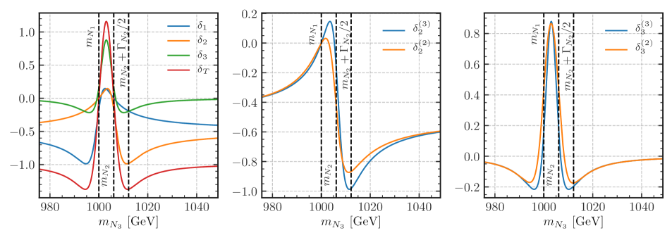
Figure 1: Left panel: CP asymmetries in the decays of $N_{1}$, $N_{2}$ and $N_{3}$, together with the total CP asymmetry $\delta_{T}=\sum_{\alpha}\delta_{\alpha}$, as a function of the mass of $N_{3}$. Centre panel: CP asymmetry in the decay of $N_{2}$ vs. $m_{N_{3}}$ as calculated in a model that considers two-neutrino mixing ($\delta^{(2)}_{2}$) and three-neutrino mixing ($\delta^{(3)}_{2}$). Right panel: CP asymmetry in the decay of $N_{3}$ vs. $m_{N_{3}}$ calculated in a model that considers two-neutrino mixing ($\delta^{(2)}_{3}$) and three-neutrino mixing ($\delta^{(3)}_{3}$). In all three panels, the vertical dashed lines indicate, from left to right, the values of $m_{N_{1}}$, $m_{N_{2}}$ and the tri-resonant value of $m_{N_{3}}$ (for details, see text).

Several applications of the RL formalism (e.g. [45, 46, 47, 48, 49, 50, 51]) exploit the bi-resonant enhancement of CP violating effects due to the mixing of two Majorana neutrinos, while the contribution to the CP asymmetry due a third singlet neutrino is either absent due to the neutrino mass model choice, or negligible when compared to the one generated in the decays of the resonating pair. However, in a model with three right-handed neutrinos, in the region where the masses of the heavy neutrinos satisfy the resonance condition

$$|m_{N_{\alpha}}-m_{N_{\beta}}|\simeq\frac{\Gamma_{N_{\alpha,\beta}}}{2}\qquad(\alpha\neq\beta),$$ (4.11)

effects of constructive interference generated by a third resonating neutrino can further enhance CP violation as compared to the case when only two neutrinos are in resonance. Figure 1 shows the behaviour of the CP asymmetries in the decays of $N_{1}$, $N_{2}$, and $N_{3}$, as well as the total CP asymmetry $\delta_{T}=\sum_{\alpha}\delta_{\alpha}$, plotted against $m_{N_{3}}$. In this figure, the mass of $N_{2}$ is fixed at the value $m_{N_{2}}=m_{N_{1}}+\Gamma_{N_{1}}/2$, therefore it fulfills the bi-resonant condition. On the left panel, it can be seen that when $m_{N_{3}}=m_{N_{2}}$, the total CP asymmetry (solid red line) vanishes due to the destructive interference effect of $N_{3}$, while at $m_{N_{3}}=m_{N_{2}}+\Gamma_{N_{2}}/2$, $|\delta_{T}|$ reaches a maximum that is more than 35% higher than in a model where the mass of the third singlet neutrino lies outside the resonance region (i.e., high $m_{N_{3}}$). In this tri-resonant point, one has $\delta_{1}\approx\delta_{3}$, while $\delta_{2}$ is the dominant contribution to $\delta_{T}$. Furthermore, we find that the values of $\delta_{1,2,3}$ are independent of the mass scale, $m_{N_{1}}$, provided that the tri-resonant condition is satisfied. Thus, the enhancement of $\delta_{2}$ is pervasive throughout the tri-resonant parameter space. The middle panel of Figure 1 shows the impact of the proper three-neutrino mixing resummation on the asymmetry $\delta_{2}$ by comparing the asymmetry calculated by considering three Majorana neutrino mixing ($\delta^{(3)}_{2}$) with the two-neutrino mixing case ($\delta^{(2)}_{2}$). When $m_{N_{3}}$ lies in the resonance region, it can be seen that the mixing with $N_{3}$ becomes important, and there is a sizeable difference between the two- and three-neutrino mixing scenarios, where the latter has a sizeable enhancement effect on $\delta_{2}$. The right panel of Figure 1 shows that the inclusion of three-neutrino mixing also affects the size of the maximum magnitude of the asymmetry in the decays of $N_{3}$, although to a lesser extent.

Overall, Figure 1 showcases a resonant enhancement of the total CP asymmetry of the model when the three heavy neutrinos are in successive resonance, a scenario that we have described as tri-resonant, in contrast to the bi-resonant approximation commonly studied in the literature. We identify a particular tri-resonant structure which generates appreciable BAU and maximises the scale of CP asymmetry within a model with three singlet neutrino mixing. In the literature, there also exist studies which consider the mixing effects of three singlet neutrinos [22, 23, 52, 53, 54, 55]. These studies utilise a flavour structure different to the $\mathbb{Z}_{6}$ structure we have adopted, and in the case of [53], it is more similar to that proposed in [56]. Hence, the flavour structure presented in these studies cannot be mapped onto the discrete flavour symmetries we have used here, so as to enable some meaningful comparison. Finally, we must point out that our approximate $\mathbb{Z}_{6}$-symmetric flavour structure provides both light neutrino masses, and the origin for CP violation.

4.2 Boltzmann Equations

The conditions for generating a BAU, dictated by [10], require not only a violation of the CP symmetry, but also a departure from thermal equilibrium and baryon number violation. Here, we introduce the set of Boltzmann equations that describe the out-of-equilibrium dynamical generation of a lepton asymmetry in the early Universe, and assume that it is reprocessed into a net baryon number through equilibrium $(B+L)$-violating sphaleron transitions [57].

At temperatures, $T$, pertinent to leptogenesis, the Universe is assumed to be radiation dominated, with an energy and entropy density given by

$$\rho(T) =\frac{\pi^{2}}{30}g_{\rm eff}(T)\,T^{4}\;,$$ (4.12)

$$s(T) =\frac{2\pi^{2}}{45}h_{\rm eff}(T)\,T^{3}\;,$$ (4.13)

respectively. Here $g_{\rm eff}$ and $h_{\rm eff}$ are the relativistic dofs of the SM plasma that correspond to $\rho$ and $s$, respectively. For our numerical results, we use the tabulated data for the relativistic dofs as calculated in [59].

The evolution of the heavy neutrino and lepton asymmetry number densities are described by their respective BEs in terms of the dimensionless parameter $z_{\alpha}=m_{N_{\alpha}}/T$, for $\alpha=1,2,3$. In line with previous conventions, we use $z=z_{1}$. These BEs are presented in [16], and due to the approximate democratic structure of the neutrino Yukawa matrix in our TRL models, we sum over lepton flavours, which leaves us with four coupled evolution equations.

Following the conventions of [16], we normalise all number densities with the photon number density

$$n_{\gamma}(z_{\alpha})=\frac{2\zeta(3)T^{3}}{\pi^{2}}=\frac{2\zeta(3)}{\pi^{2}}\left(\dfrac{m_{N_{\alpha}}}{z_{\alpha}}\right)^{3},$$ (4.14)

which for a given particle species $i$, gives us the ratio

$$\eta_{i}(z_{\alpha}) =\frac{n_{i}(z_{\alpha})}{n_{\gamma}(z_{\alpha})}\;.$$ (4.15)

In addition, we define the departure from equilibrium for the heavy-neutrino density as

$$\delta\eta_{N_{\alpha}}(z_{\alpha}) =\frac{\eta_{N_{\alpha}}(z_{\alpha})}{\eta_{N_{\alpha}}^{\rm eq}(z_{\alpha})}-1\;,$$ (4.16)

where $\eta_{N_{\alpha}}^{\rm eq}$ denotes $\eta_{N_{\alpha}}$ in thermal equilibrium, for which we use the approximate expression

$$\eta_{N_{\alpha}}^{\rm eq}(z_{\alpha})\approx\frac{z_{\alpha}^{2}}{2\zeta(3)}K_{2}(z_{\alpha}).$$ (4.17)

Here, $\zeta(3)\approx 1.202$ is Apéry’s constant, and $K_{n}(z)$ is a modified Bessel function of the second kind. In the BEs, we have also included terms which depend on the parameter

$$\delta_{h}(z_{\alpha})=1-\dfrac{1}{3}\dfrac{d\ln h_{\rm eff}}{d\ln z_{\alpha}}\;,$$ (4.18)

since we allow $h_{\textrm{eff}}$ to vary with $T$.

Considering decay terms, $\Delta L=1$ and $\Delta L=2$ scattering processes, and the running of the dof parameters, the BEs can be written as

$$\frac{d\delta\eta_{N_{\alpha}}}{d\ln z_{\alpha}}= -\dfrac{\delta_{h}(z_{\alpha})}{H(z_{\alpha})\ \eta_{N_{\alpha}}^{\rm eq}(z_{\alpha})}\left[\delta\eta_{N_{\alpha}}\left(\Gamma^{D(\alpha)}+\Gamma^{S(\alpha)}_{Y}+\Gamma^{S(\alpha)}_{G}\right)+\frac{2}{9}\,\eta_{L}\,\delta_{\alpha}\left(\tilde{\Gamma}^{D(\alpha)}+\hat{\Gamma}^{S(\alpha)}_{Y}+\hat{\Gamma}^{S(\alpha)}_{G}\right)\right]$$

$$+\left(\delta\eta_{N_{\alpha}}+1\right)\,\left[z_{\alpha}\frac{K_{1}(z_{\alpha})}{K_{2}(z_{\alpha})}-3(\delta_{h}(z_{\alpha})-1)\right]\;,$$ (4.19)

$$\frac{d\eta_{L}}{d\ln z}= -\frac{\delta_{h}(z)}{H(z)}\Bigg{\{}\sum_{\alpha=1}^{3}\delta\eta_{N_{\alpha}}\delta_{\alpha}\left(\Gamma^{D(\alpha)}+\Gamma^{S(\alpha)}_{Y}+\Gamma^{S(\alpha)}_{G}\right)$$

$$+\frac{2}{9}\eta_{L}\left[\sum_{\alpha=1}^{3}\left(\tilde{\Gamma}^{D(\alpha)}+\tilde{\Gamma}^{S(\alpha)}_{Y}+\tilde{\Gamma}^{S(\alpha)}_{G}+\Gamma^{W(\alpha)}_{Y}+\Gamma^{W(\alpha)}_{G}\right)+\Gamma^{\Delta L=2}\right]$$

$$+\dfrac{2}{27}\eta_{L}\,\sum_{\alpha=1}^{3}\delta_{\alpha}^{2}\,\left(\Gamma^{W(\alpha)}_{Y}+\Gamma^{W(\alpha)}_{G}\right)\Bigg{\}}-3\eta_{L}(\delta_{h}(z)-1)\;,$$ (4.20)

where

$$H(z_{\alpha})=\sqrt{\frac{4\pi^{3}g_{\textrm{eff}}(z_{\alpha})}{45}}\frac{m_{N_{\alpha}}^{2}}{M_{\textrm{Pl}}}\frac{1}{z_{\alpha}^{2}}$$ (4.21)

is the Hubble parameter, and $M_{\textrm{Pl}}\approx 1.221\times 10^{19}~{}{\rm GeV}$ is the Planck mass. Since the BEs are not identical to the ones utilised in the literature due to the non-trivial $T$-dependence of $h_{\rm eff}$, we show how they are obtained in Appendix A. The various collision terms are defined in the literature [16] as

$$\Gamma^{D(\alpha)} =\frac{1}{n_{\gamma}}\gamma^{N_{\alpha}}_{L\Phi},$$ (4.22)

$$\tilde{\Gamma}^{D(\alpha)} =\left(1+\dfrac{12}{21}\right)\Gamma^{D(\alpha)},$$ (4.23)

$$\Gamma^{S(\alpha)}_{Y} =\frac{1}{n_{\gamma}}\left[\gamma^{N_{\alpha}L}_{Qu^{C}}+2\gamma^{N_{\alpha}u^{C}}_{LQ^{C}}\right],$$ (4.24)

$$\tilde{\Gamma}^{S(\alpha)}_{Y} =\frac{1}{n_{\gamma}}\left[\left(\delta\eta_{N_{\alpha}}+1+\dfrac{12}{21}\right)\gamma^{N_{\alpha}L}_{Qu^{C}}+\left(2+\dfrac{98}{159}(\delta\eta_{N_{\alpha}}+2)\right)\gamma^{N_{\alpha}u^{C}}_{LQ^{C}}\right],$$ (4.25)

$$\hat{\Gamma}^{S(\alpha)}_{Y} =\frac{1}{n_{\gamma}}\left[\left(-(\delta\eta_{N_{\alpha}}+1)+\dfrac{12}{21}\right)\gamma^{N_{\alpha}L}_{Qu^{C}}+\left(2-\dfrac{98}{159}\delta\eta_{N_{\alpha}}\right)\gamma^{N_{\alpha}u^{C}}_{LQ^{C}}\right],$$ (4.26)

$$\Gamma^{S(\alpha)}_{G} =\frac{1}{n_{\gamma}}\left[\gamma^{N_{\alpha}V_{\mu}}_{L\Phi}+\gamma^{N_{\alpha}L}_{V_{\mu}\Phi^{\dagger}}+\gamma^{N_{\alpha}\Phi^{\dagger}}_{LV_{\mu}}\right],$$ (4.27)

$$\tilde{\Gamma}^{S(\alpha)}_{G} =\frac{1}{n_{\gamma}}\left[\left(1+\dfrac{12}{21}\right)\gamma^{N_{\alpha}V_{\mu}}_{L\Phi}+\left(\delta\eta_{N_{\alpha}}+1+\dfrac{12}{21}\right)\gamma^{N_{\alpha}L}_{V_{\mu}\Phi^{\dagger}}+\left(1+(\delta\eta_{N_{\alpha}}+1)\dfrac{12}{21}\right)\gamma^{N_{\alpha}\Phi^{\dagger}}_{LV_{\mu}}\right],$$ (4.28)

$$\hat{\Gamma}^{S(\alpha)}_{G} =\frac{1}{n_{\gamma}}\left[\left(1+\dfrac{12}{21}\right)\gamma^{N_{\alpha}V_{\mu}}_{L\Phi}+\left(-(\delta\eta_{N_{\alpha}}+1)+\dfrac{12}{21}\right)\gamma^{N_{\alpha}L}_{V_{\mu}\Phi^{\dagger}}+\left(1-(\delta\eta_{N_{\alpha}}+1)\dfrac{12}{21}\right)\gamma^{N_{\alpha}\Phi^{\dagger}}_{LV_{\mu}}\right],$$ (4.29)

$$\Gamma^{W(\alpha)}_{Y} =\frac{1}{n_{\gamma}}\left[\left(2+\dfrac{12}{21}\right)\gamma^{N_{\alpha}L}_{Qu^{C}}+\left(2+\dfrac{12}{7}\right)\gamma^{N_{\alpha}u^{C}}_{LQ^{C}}\right],$$ (4.30)

$$\Gamma^{W(\alpha)}_{G} =\frac{1}{n_{\gamma}}\left[\left(1+\dfrac{12}{21}\right)\gamma^{N_{\alpha}V_{\mu}}_{L\Phi}+\left(2+\dfrac{12}{21}\right)\gamma^{N_{\alpha}L}_{V_{\mu}\Phi^{\dagger}}+\left(1+\dfrac{24}{21}\right)\gamma^{N_{\alpha}\Phi^{\dagger}}_{LV_{\mu}}\right],$$ (4.31)

$$\Gamma^{\Delta L=2} =\frac{2}{n_{\gamma}}\left(1+\dfrac{12}{21}\right)\left[{\gamma^{\prime}}^{L\Phi}_{L^{C}\Phi^{\dagger}}+\gamma^{LL}_{\Phi^{\dagger}\Phi^{\dagger}}\right],$$ (4.32)

where $\gamma^{X}_{Y}$ are CP-conserving collision terms for the process ${X\rightarrow Y}$. The latter is defined as

$$\gamma^{X}_{Y}\equiv\gamma(X\rightarrow Y)+\gamma(\overline{X}\rightarrow\overline{Y}),$$ (4.33)

where the bar denotes CP conjugation. The pertinent analytical expressions of the collision terms and scattering cross sections can all be found in [16]. Note that the primed terms correspond to collision terms with subtracted real intermediate states (RIS), which can take negative values due to the lack of an on-shell contribution to the squared amplitude.

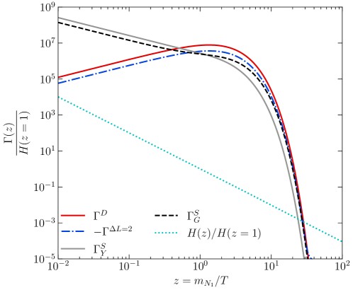
Figure 2: The $\delta\eta_{N_{\alpha}}$ independent collision terms are defined in (4.32) for $|{\bf h}^{\nu}_{ij}|\approx 3\times 10^{-3}$ and $m_{N_{1}}=500~{}{\rm GeV}$. The wash-out terms, $\Gamma^{W}_{Y,G}$, are uniformly different by a factor of two compared to their source ($\Gamma^{S}_{Y,G}$) counterparts.

The typical dependence of the various collision terms on $z=m_{N_{1}}/T$ is shown in Figure 2, for $|{\bf h}^{\nu}_{ij}|\approx 3\times 10^{-3}$ and $m_{N_{1}}=500~{}{\rm GeV}$. The other two masses obey the tri-resonant condition, which results in a sizeable $\Delta L=2$ rate. It is noteworthy that the collision term that describes the decays and the RIS parts is larger than $\Gamma^{\Delta L=2}$, as also observed in [13]. For this figure, the relevant perturbation matrix, $\delta{\bf h}^{\nu}$, needed to match the neutrino data may be found in Appendix C under Benchmark A.

During leptogenesis, part of the lepton asymmetry that is generated in the processes described above is partially converted into a baryon asymmetry by $(B+L)$-violating sphaleron transitions which become exponentially suppressed below the temperature $T_{\rm sph}\simeq 132$ GeV [71]. In order to compare the generated BAU at $T=T_{\rm sph}$ to its value at the recombination epoch, we assume that there are no considerable entropy releasing processes, and hence the entropy density remains approximately constant as the Universe cools. Using entropy conservation and the relation ${s(T)\sim h_{\textrm{eff}}(T)\,T^{3}}$, it can be shown that the BAU at $T_{\textrm{sph}}$ is related to the BAU at $T_{\textrm{rec}}$ by

$$\eta^{\rm rec}_{B}=\frac{h_{\rm eff}(T_{\rm rec})}{h_{\rm eff}(T_{\rm sph})}\frac{n_{B}(T_{\rm sph})}{n_{\gamma}(T_{\rm sph})}=f\frac{n_{B}(T_{\rm sph})}{n_{\gamma}(T_{\rm sph})}\;.$$ (4.34)

For the dilution factor, $f$, we use the approximate value $1/27$ [72, 13], while for the conversion factor between lepton and baryon number above the sphaleron temperature, we use the equilibrium relation given by [73]

$$\eta_{B}=-\frac{28}{51}\eta_{L}\;.$$ (4.35)

5 Approximate Solutions to Boltzmann Equations

In this section we discuss the solution of the BEs (4.19) and (4.20) in order to understand the production of a lepton asymmetry in the early Universe. As a first approach, we consider a simplified version of these equations, where we ignore the “back-reaction” (i.e. the second term of (4.19)), the variation of the relativistic dofs, and only take into account the decay and RIS terms. Moreover, we assume that $m_{N_{1}}\approx m_{N_{2}}\approx m_{N_{3}}$.

5.1 Approximation for $\delta\eta_{N_{\alpha}}$

We begin by solving the equation for $\delta\eta_{N_{\alpha}}$, which takes the form

$$\dfrac{d\delta\eta_{N_{\alpha}}}{dz}=\dfrac{K_{1}(z)}{K_{2}(z)}\left[1+\left(1-z\dfrac{\Gamma_{N_{\alpha}}}{H(z=1)}\right)\ \delta\eta_{N_{\alpha}}\right]\;.$$ (5.1)

Initially (at $z\ll 1$), right-handed neutrinos are taken to be in thermal equilibrium, so $\delta\eta_{N_{\alpha}}=0$. Therefore, at early times, we expect the second term of (5.1) to vanish. Moreover, at such high temperatures, we may approximate ${K_{1}(z)/K_{2}(z)\approx z/2}$, so

$$\delta\eta_{N_{\alpha}}\approx\dfrac{z^{2}}{4}\,,\qquad\text{for }z\ll 1\;.$$ (5.2)

As the temperature drops, $\delta\eta_{N_{\alpha}}$ increases, and at some point the second term starts to become comparable to the first. So, $\delta\eta_{N_{\alpha}}$ continues to increase until both terms become equal. We denote this point as $z=\hat{z}$, and assuming $\hat{z}\gg H(z=1)/\Gamma_{N_{\alpha}}$, it is estimated as

$$\hat{z}\approx\left(\dfrac{4\,H(z=1)}{\Gamma_{N_{\alpha}}}\right)^{1/3}\;.$$ (5.3)

For $z\approx\hat{z}$, we observe that the RHS of (5.1) stays close to zero. That is, $\delta\eta_{N_{\alpha}}\approx H(z=1)/\Gamma_{N_{\alpha}}z^{-1}$, since any increase (decrease) with respect to this behaviour pushes $\delta\eta_{N_{\alpha}}$ to negative (positive) values. Consequently, we find that for $z\gg\hat{z}$,

$$\delta\eta_{N_{\alpha}}\approx\dfrac{H(z=1)}{\Gamma_{N_{\alpha}}z}\;.$$ (5.4)

Notice that this result does not depend on the initial condition. Also, we should point out that at late times, namely $z\gg 1$, (5.4) solves (5.1) up to terms $\mathcal{O}(1/z^{2})$.

5.1.1 The Neutrino Boltzmann Equation as an Autonomous System

The independence from the initial conditions has been previously highlighted in the literature (e.g. [16, 22]). However, it would be helpful to analyse its attractor properties. We begin by noting that (5.1) can be written in the form of an autonomous system

$$\dfrac{d\mathbf{r}}{dt}=\mathbf{V}\left(z(t),\delta\eta_{N_{\alpha}}(t)\right)\;,$$ (5.5)

with $\mathbf{r}=(z,\delta\eta_{N_{\alpha}})^{\sf T}$ and

$$\mathbf{V}\left(z(t),\delta\eta_{N_{\alpha}}(t)\right)=\left(\begin{matrix}1\\[8.5359pt] \dfrac{K_{1}(z(t))}{K_{2}(z(t))}\left[1+\left(1-z(t)\dfrac{\Gamma_{N_{\alpha}}}{H(z=1)}\right)\ \delta\eta_{N_{\alpha}}(t)\right]\end{matrix}\right).$$ (5.6)

Here, the vector field $\mathbf{V}$ represents the flow of (5.1), which helps to demonstrate how $\mathbf{r}$ reaches the stable solution, independently of the initial conditions. In Figure 3, we show the evolution of $\delta\eta_{N_{\alpha}}$ for $\Gamma_{N_{\alpha}}=100\,H(z=1)$ and for two different initial conditions. Along with the two curves, we show the direction of $\mathbf{V}$, which indicates at each point the tendency of $\mathbf{r}$. Moreover, darker arrows imply higher values of $\left|d\delta\eta_{N_{\alpha}}/dz\right|$. As both curves merge at $z\gtrsim\hat{z}$, $\delta\eta_{N_{\alpha}}$ ends up becoming ignorant of the initial condition. This feature is also imprinted in the direction of $\mathbf{V}$. The normalised vector, $\mathbf{V}$, is parallel to the $z$-axis for $z\lesssim\hat{z}$, while it points towards the solution for $z\gtrsim\hat{z}$.

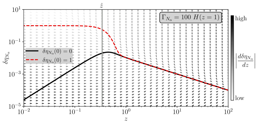
Figure 3: The solution of (5.1) for $\Gamma_{N_{\alpha}}=100\ H(z=1)$ with initial conditions $\delta\eta_{N_{\alpha}}(z\to 0)=0$ (black) and $\delta\eta_{N_{\alpha}}(z\to 0)=1$ (dashed red). The arrows show the direction of $\mathbf{V}$, while the colour gradient encodes the size of $\delta\eta_{N_{\alpha}}$, with light grey (black) for low (high) values of $\left|d\delta\eta_{N_{\alpha}}/dz\right|$. The vertical grey line shows the value of $\hat{z}$ as estimated by (5.3).

5.2 Approximation for $\eta_{L}$

The corresponding equation for the lepton asymmetry, assuming that $\delta\eta_{N_{\alpha}}\sim 1/z$, can be written as

$$\dfrac{d\eta_{L}}{dz}=\dfrac{\delta_{T}}{2\zeta(3)}K_{1}(z)\,z^{2}\ \left(1-z\,\dfrac{2k_{L}}{3\delta_{T}}\eta_{L}\right)\;,$$ (5.7)

where $\delta_{T}=\sum_{\alpha}\delta_{\alpha}$ and $k_{L}=\displaystyle\sum_{a}\dfrac{\Gamma_{N_{\alpha}}}{H(z=1)}$.

Initially, at $z\ll 1$, the lepton asymmetry is assumed to vanish. So, at high temperatures, only the first term of (5.7) contributes. Therefore, since $K_{1}(z)z^{2}\approx z$, $\eta_{L}\approx\delta_{T}/\left(4\zeta(3)\right)\,z^{2}$. As $\eta_{L}$ increases, both terms become comparable at

$$z=\tilde{z}\approx 2k_{L}^{-1/3}\;.$$ (5.8)

After this point, the RHS of (5.7) remains close to zero, as in the previous case. Hence,

$$\eta_{L}\approx\dfrac{3\delta_{T}}{2k_{L}\,z}\;.$$ (5.9)

However, at very low temperatures, $z\gg 1$, the RHS of (5.7) becomes exponentially suppressed, due to the asymptotic behaviour $K_{1}(z\ll 1)\sim e^{-z}$. Then, the lepton asymmetry becomes a constant, i.e. $\eta_{L}$ freezes out at some $z=z_{\rm fo}$. This point can be estimated by demanding that the rate at which $\eta_{L}$ changes is comparable to its magnitude, which implies that

$$\dfrac{k_{L}}{3\zeta(3)}\sqrt{\dfrac{\pi}{2}}e^{-z_{\rm fo}}\ z_{\rm fo}^{5/2}\approx 1\;.$$ (5.10)

This equation can be solved using fixed point iteration. Keeping the first two iterations, we estimate

$$z_{\rm fo}\approx\ln(3k_{L})+5/2\ln(\ln(3k_{L}))+\mathcal{O}\left(\ln\ln\ln k_{L}\right)\;.$$ (5.11)

At lower temperatures, with $z>z_{\rm fo}$, the lepton asymmetry becomes

$$\eta_{L}\approx\dfrac{3\delta_{T}}{2k_{L}\,z_{\rm fo}}\;.$$ (5.12)

As before, we note that this solution is independent of any initial asymmetry that might have existed before the one generated by the heavy Majorana neutrino decays.

5.2.1 The Baryon Asymmetry

Using (4.34) and (4.35) and assuming that the freeze-out happens before $z=z_{\rm sph}$, i.e. $z_{\rm fo}>m_{N_{\alpha}}/T_{\rm sph}$, the predicted baryon asymmetry at the time of recombination reads

$$\eta_{B}\sim-3\times 10^{-2}\ \displaystyle\dfrac{\delta_{T}}{k_{L}\left[\ln(3k_{L})+5/2\ln(\ln(3k_{L}))\right]}\;.$$ (5.13)

However, if $z_{\rm fo}<m_{N_{\alpha}}/T_{\rm sph}$, the baryon asymmetry becomes

$$\eta_{B}\sim-3\times 10^{-2}\ \displaystyle\dfrac{\delta_{T}}{k_{L}z_{\rm sph}}\;.$$ (5.14)

It should be noted that the resulting value of $\eta_{L}$ is proportional to $\delta_{T}/[k_{L}\ln(3k_{L})]$, with the logarithmic dependence coming from the determination of the freeze-out temperature. This means that, generally, for a given value of $k_{L}$, only $\delta_{T}$ determines the baryon asymmetry. In particular, for $k_{L}>10$, the observed baryon asymmetry can be obtained for $\delta_{T}\gtrsim 10^{-7}$.

5.2.2 The Lepton Asymmetry Boltzmann Equation as an Autonomous System

The lepton asymmetry BE (5.7) can also be written as an autonomous system

$$\dfrac{d\mathbf{r}}{dt}=\mathbf{V}\Big{(}z(t),\eta_{L}(t)\Big{)}\;,$$ (5.15)

with $\mathbf{r}=(z,\eta_{L})^{\textsf{T}}$ and

$$\mathbf{V}\Big{(}z(t),\eta_{L}(t)\Big{)}=\left(\begin{matrix}1\\[8.5359pt] \dfrac{\delta_{T}}{2\zeta(3)}K_{1}(z(t))\,z^{2}(t)\ \left(1-z(t)\,\dfrac{2k_{L}}{3\delta_{T}}\eta_{L}(t)\right)\end{matrix}\right)\;.$$ (5.16)

This system is similar to (5.6), but it also exhibits a freeze-out. We can observe the evolution of $\eta_{L}$ in Figure 4, where we show the flow of the autonomous system of (5.15), along with its solution for two initial conditions.

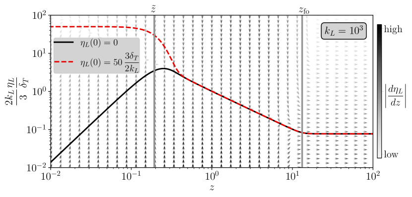
Figure 4: The solution of (5.7) for $k_{L}=100$ with initial conditions $\eta_{L}(z\to 0)=0$ (black) and $\eta_{L}(z\to 0)=50\,(3\delta_{T}/2k_{L})$ (dashed red). The arrows show the direction of $\mathbf{V}$, while the colour gradient encodes the size of the LHS relative to $\eta_{L}$; from light grey for low values to darker grey for higher values. The two vertical (grey) lines show the values of $z=\tilde{z}$ and $z=z_{\rm fo}$ as approximated in (5.8) and (5.11), respectively.

We note that the derivative of $\eta_{L}$ can only deviate significantly from zero in the range $\tilde{z}\lesssim z\lesssim z_{\rm fo}$. This is the period in which $d\eta_{L}/dz$ pushes the solution towards $\eta_{L}\sim 1/z$, as below (above) this curve $\mathbf{V}$ points upwards (downwards), with significant magnitude. Notice that in the region $z\gtrsim z_{\rm fo}$, $\mathbf{V}$ points towards the right. This means that the component that dominates $\mathbf{V}$ is $dz/dt=1$. Thus, the flow of (5.15) will only follow $z$, as $d\eta_{L}/dz$ gets exponentially suppressed.

5.3 Numerical Approximation of the Complete Boltzmann
Equations

Although (5.1) and (5.7) are very different than their more accurate counterparts, i.e. the BEs (4.19) and (4.20), they show that their solutions mostly follow the lines that cause the RHS to approximately vanish. In other words, they follow “attractor” solutions. The same argument used to show this for (5.1) and (5.7) can be applied to (4.19) and (4.20). Assuming that the $\eta_{L}$-dependent term of (4.19) is suppressed (i.e. $\delta_{\alpha}\ll 1$), we can estimate the evolution of both $\delta\eta_{N_{\alpha}}$ and $\eta_{L}$ by demanding the vanishing of the RHS of (4.19) and (4.20). Although such an estimation can only be done numerically, it can still be helpful as it shows that the initial conditions do not change the lepton asymmetry at low temperatures.

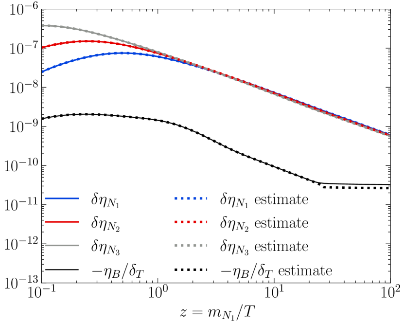
(a)

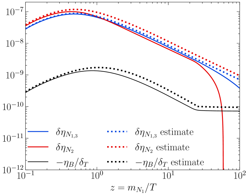
(b)

Figure 5: Numerical and approximate solutions of the BEs (4.19) and (4.20) for two points in our parameter space with $m_{N_{1}}=m_{N_{2}}/2=m_{N_{3}}/4=700~{}{\rm GeV}$ (left) and $m_{N_{3}}\approx m_{N_{2}}\approx m_{N_{1}}=700~{}{\rm GeV}$ (right), and $|{\bf h}^{\nu}_{ij}|\approx 3\times 10^{-4}$. The lines correspond to the numerical solutions for $\delta_{N_{1}}$ (blue), $\delta_{N_{2}}$ (red), $\delta_{N_{3}}$ (grey), and $\eta_{L}/\delta_{1}$ (black), while the dotted lines of the same colour show the corresponding estimate.

In Figure 5(a), we show the solution of the BEs (4.19) and (4.20) for $m_{N_{1}}=700~{}{\rm GeV}$, $m_{N_{2}}=1.4~{}{\rm TeV}$, $m_{N_{3}}=2.8~{}{\rm TeV}$, and $|{\bf h}^{\nu}_{ij}|\approx 3\times 10^{-4}$. We note that this is away from the resonant region, so $\delta_{T}\ll 1$. As this results in a suppressed back-reaction term of (4.19), the numerical estimates turn out to agree with the numerical solution of the BEs, even at high temperatures. This suggests that the addition of the $2\to 2$ processes pushes the system towards its attractor solution faster. Finally, as can be seen, the freeze-out is not identified correctly, and the resulting baryon asymmetry is slightly underestimated.

For scenarios with large $\delta_{\alpha}$, the approximation deviates from the attractor solution, as the BEs (4.19) and (4.20) are no longer independent due to the lepton back-reaction contribution to (4.19). In Figure 5(b) we show the evolution of $\delta\eta_{N_{\alpha}}$ and $\eta_{B}$ for $m_{N_{1}}=700~{}{\rm GeV}$ (with $m_{N_{2,3}}$ satisfying the tri-resonant condition (4.11)) and $|{\bf h}^{\nu}_{ij}|\approx 3\times 10^{-4}$, which results in $\delta_{T}\sim-1$ (Benchmark $\mathbf{B}$ in Appendix C). In turn, the back-reaction term in (4.19) gives a non-trivial contribution to the evolution of $\delta\eta_{N_{\alpha}}$. Consequently, for $z\gg 1$, $\delta\eta_{N_{1,2,3}}$ decrease at a higher rate, resulting in a discrepancy between the numerical and approximate solutions. Note that, as shown in Figure 1, we have $\delta_{1}\approx\delta_{3}$, while $\delta_{2}$ yields the dominant contribution to the CP asymmetry. This is reflected in Figure 5(b), as $\delta\eta_{N_{2}}$ begins to fall at lower $z$ than $\delta\eta_{N_{1,3}}$.

5.3.1 The Effect of Varying Relativistic Degrees of Freedom

As already mentioned, we have taken into account the temperature dependence of the effective relativistic dofs of the plasma, which introduces a dependence on $d\ln h_{\rm eff}/d\ln T$ in both (4.19) and (4.20). In Figure 6 we show $d\ln h_{\rm eff}/d\ln T$ as a function of the temperature in the range $100~{}{\rm GeV}\leq T\leq 10~{}{\rm TeV}$. The two lines correspond to the tabulated values given in [59] (in black) and [74] (in blue).

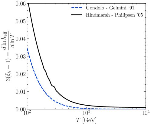
Figure 6: The derivative of $\ln h_{\rm eff}$ with respect to $\ln T$ for $100~{}{\rm GeV}\leq T\leq 10~{}{\rm TeV}$. The black (solid) line corresponds to the tabulated values of $h_{\rm eff}$ given in [59], while the blue (dashed) line corresponds to [74].

Despite the seemingly small deviation from zero, the effect of a non-vanishing derivative of $h_{\rm eff}$ is, in general, not negligible. In particular, for $\delta_{h}>1$ the last term of (4.19) can dominate, which can result in a negative $\delta\eta_{N_{\alpha}}$. If this happens at temperatures close to $T_{\rm sph}$, $\delta\eta_{N_{\alpha}}$ does not have time to “bounce” to positive values. Then, since $\eta_{L}$ depends on $\delta\eta_{N_{\alpha}}$, $\eta_{B}$ can also obtain a negative value at $T=T_{\rm sph}$.

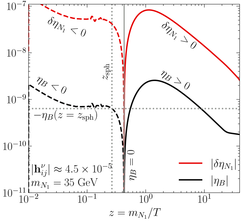
(a)

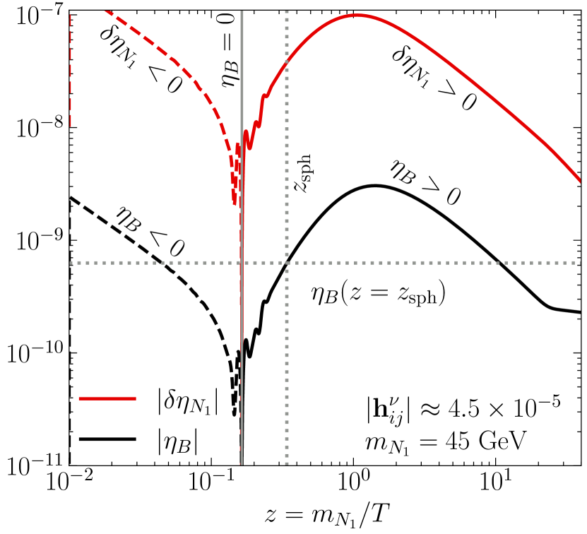
(b)

Figure 7: Evolution of $\delta_{N_{1}}$ (red) and $\eta_{L}$ (black) for $m_{N_{1}}=35~{}{\rm GeV}$ (a) and $m_{N_{1}}=45~{}{\rm GeV}$ (b), and $|{\bf h}^{\nu}_{ij}|\approx 4.5\times 10^{-5}$. The black and red solid (dashed) lines show where $\eta_{B}$ and $\delta_{N_{1}}$are positive (negative), the solid grey lines shows the points where $\eta_{B}=0$. The vertical dotted grey lines correspond to $z_{\rm sph}=m_{N_{1}}/T_{\rm sph}$, while the horizontal ones show the value of $|\eta_{B}|$ at $z=z_{\rm sph}$.

This behaviour is observed in Figure 7, where we show the evolution of $\delta_{N_{1}}$ (in red) and $\eta_{L}$ (in black) for $m_{N_{1}}=35~{}{\rm GeV}$ (Figure 7(a)) and $m_{N_{1}}=45~{}{\rm GeV}$ (Figure 7(b)). In both Figures 7(a) and 7(b), the solid (dashed) lines show the regime where the corresponding quantities are positive (negative), and the vertical solid grey lines show the points where $\eta_{B}=0$. The vertical dashed grey line corresponds to $T=T_{\rm sph}$, while the horizontal one displays the value of $\eta_{B}$ at $z=z_{\rm sph}$. We observe that, although the curves in both figures are similar, the prediction for the baryon asymmetry is considerably different. Particularly, in both Figures 7(a) and 7(b), the quantities are negative for $z\ll 1$ and they change sign close to $z\sim 10^{-1}$. For $m_{N_{1}}=35~{}{\rm GeV}$, this sign change would occur after the sphalerons decouple. Therefore the generated BAU is negative. Conversely, for $m_{N_{1}}=45~{}{\rm GeV}$, the sphaleron freeze-out occurs after $\eta_{B}$ becomes positive, and thus the generated BAU is positive. Moreover, we should note that this behaviour is stable under perturbing the initial conditions of both $\delta\eta_{N_{\alpha}}$ and $\eta_{L}$, as the system reaches quickly its attractor solution.

Therefore, there seems to be a mass scale, below which the resulting $\eta_{B}$ is negative, which also depends on the values of $h_{\rm eff}$ and its derivative.

(a)

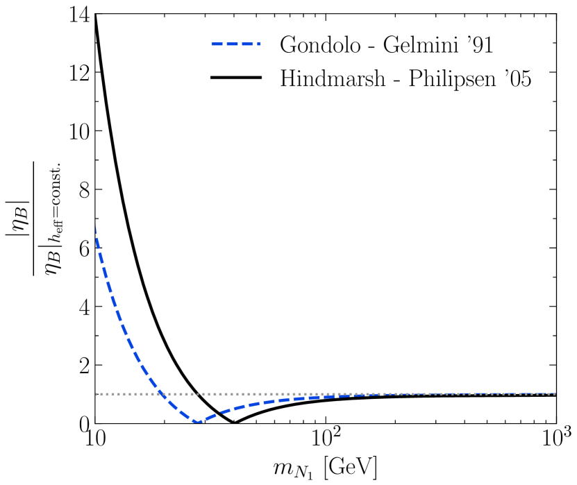
(b)

Figure 8: Left panel: The resulting $\eta_{B}$ for $|{\bf h}^{\nu}_{ij}|\approx 3\times 10^{-4}$ in the tri-resonant scenario as a function of $m_{N_{1}}$ for $h_{\rm eff}$ as given in [59] (black), [74] (blue), and taking $h_{\rm eff}={\rm const.}\approx 105$ (red). The grey dotted line shows $\eta_{B}^{\rm CMB}=6.104\times 10^{-10}$. Right panel: The ratio of $|\eta_{B}|$ with varying $h_{\rm eff}$, the black (blue) line corresponds to [59] ([74]), with respect to $h_{\rm eff}={\rm const.}$ The grey dotted line indicates $|\eta_{B}|/\eta_{B}|_{h_{\rm eff}={\rm const.}}=1$.

In Figure 8(a) we show the dependence of $\eta_{B}$ for $|{\bf h}^{\nu}_{ij}|\approx 3\times 10^{-4}$ in the tri-resonant scenario using three different forms of $h_{\rm eff}$: (i) using data given in [59] (in black), (ii) the tabulated $h_{\rm eff}$ provided in [74] (in blue), and (iii) taking $h_{\rm eff}={\rm const.}\approx 105$ (in red). We observe that $\eta_{B}$ depends heavily on the derivative of $h_{\rm eff}$ for $m_{N_{1}}\lesssim 100~{}{\rm GeV}$. In particular, the commonly used assumption, $h_{\rm eff}={\rm const.}$, results in overall larger baryon asymmetry today, while the cases with varying $h_{\rm eff}$ are lower. In fact, larger values of $d\ln h_{\rm eff}/d\ln T$ imply a smaller $\eta_{B}$. Moreover, at around $m_{N_{1}}=40~{}{\rm GeV}$, $\eta_{B}$ becomes negative, which means that this is a scale below which the CP asymmetries need to change their sign. A positive $\eta_{B}$ can be obtained by changing $\mathbf{h}_{+}^{\nu}$ to its CP conjugate, e.g. by $\omega\to\omega^{*}$. We should stress that the regime $m_{N_{1}}\lesssim 100~{}{\rm GeV}$ needs to be carefully studied along with the values of $h_{\rm eff}$ at temperatures larger than $T_{\rm sph}$, as the baryon asymmetry is very sensitive on the derivative of $h_{\rm eff}$. This sensitivity can also be seen in Figure 8(b), where we show the ratio between $|\eta_{B}|$ with varying $h_{\rm eff}$ (again, black corresponds to [59] and blue to [74]) with respect to $h_{\rm eff}={\rm const}$. In this figure, we observe again that $m_{N_{1}}\lesssim 100~{}{\rm GeV}$ is sensitive to the derivative of $h_{\rm eff}$, as both lines deviate considerably from $1$ as well as from each other by a factor of $\sim 2$ for $m_{N_{1}}\lesssim 40~{}{\rm GeV}$. In the regime $m_{N_{1}}\lesssim 40~{}{\rm GeV}$, the baryon asymmetry would receive contributions from other effects, e.g., from coherent heavy neutrino oscillations [75, 76, 77, 78, 79, 80, 81, 82]. The impact of the derivative of $h_{\rm eff}$ on the dynamics of the baryon asymmetry would not be affected by the inclusion of these effects, as they would introduce another source of CP asymmetry at most comparable to the one considered in the BE (4.20). As a consequence, previous analyses that do not take the effect of $d\ln h_{\rm eff}/d\ln T$ into account must be revisited accordingly.

6 Results

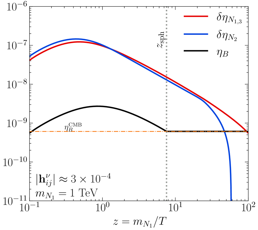
(a)

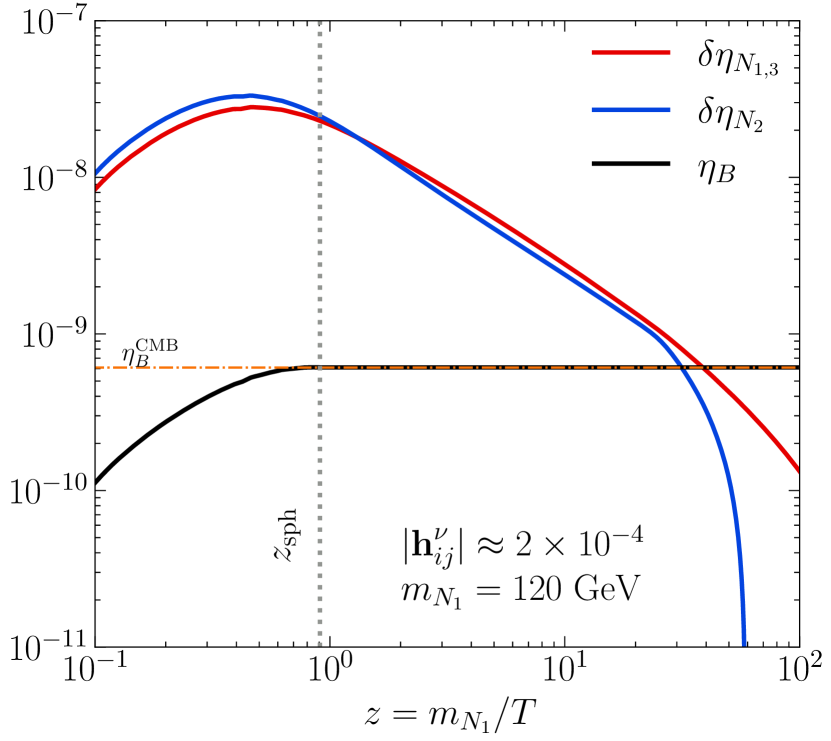
(b)

Figure 9: Evolution plots for the baryon asymmetry $\eta_{B}$ (black solid line) and the deviation from equilibrium of the neutrino densities $\delta\eta_{N_{\alpha}}$ (blue and red solid lines). The choice for the values of the mass of the lightest singlet neutrino and the scale of the Yukawa coupling can be seen on each panel, and the grey (dotted) line indicates the value $z=z_{\rm sph}$ at which the sphaleron processes freeze out. The orange dot-dashed line indicates the observed value of the baryon asymmetry of $\eta^{\rm CMB}_{B}=6.104\times 10^{-10}$.

We present the numerical solutions to the BEs as shown in (4.19) and (4.20) for the benchmark model defined by the rescaled Yukawa matrix presented in (2.17), and for a tri-resonant singlet neutrino spectrum. In the following analysis, we restrict ourselves to heavy neutrino masses above $40~{}{\rm GeV}$. Below this mass scale, our approach is more limited due to the fact that by ignoring thermal masses, we do not account for phase space suppression effects and their impact on the leptonic asymmetries. Besides these thermal effects, a more detailed treatment [81, 83, 84, 85, 86, 87] would require us to incorporate additional CP violating effects induced by the coherent oscillation of heavy neutrinos [75, 76, 77, 78, 80, 82], along with those effects that come from their CP-violating decays [12, 42, 13]. Finally, we note that for low singlet neutrino masses, the necessary CP violation could originate from Higgs decays into a singlet neutrino and a lepton doublet when the thermal effects of the plasma are considered [79, 88].

As discussed in the previous section, the scattering terms generate a delay in the onset of the maximum of the baryon asymmetry, which modifies the shape of the curve for the baryon asymmetry evolution depending on the mass of the singlet neutrinos. Figure 9(a) shows the evolution of the baryon asymmetry for $|{\bf h}^{\nu}_{ij}|=3\times 10^{-4}$ and $m_{N_{1}}=1~{}{\rm TeV}$ (labeled as Benchmark C in Appendix C), and it demonstrates that for ${\rm TeV}$ singlet neutrinos, the baryon asymmetry is reached by the freeze-out of the lepton asymmetry after the maximum value is reached. Figure 9(b) presents the evolution for $|{\bf h}^{\nu}_{ij}|=2\times 10^{-4}$ and $m_{N_{1}}=120~{}{\rm GeV}$ (Benchmark D in Appendix C), and illustrates how the generation of the baryon asymmetry happens at the maximum when the mass of the heavy neutrinos becomes lower. In both panels, we selected the initial conditions $\eta_{L}(z_{0})=0$ and $\delta\eta_{N_{\alpha}}(z_{0})=0$ for $\alpha=1,2,3$, with $z_{0}=10^{-2}$. However, due to the attractive nature of the solution to the BEs, the evolution of the baryon asymmetry remain effectively unchanged for any other reasonable choice. Also, since $\delta_{2}$ is the largest CP asymmetry, $\delta\eta_{N_{2}}$ deviates significantly from $\delta\eta_{N_{1,3}}$ at high values of $z$, as outlined in Section 5.

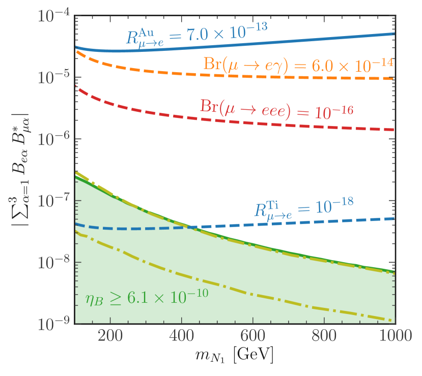
(a)

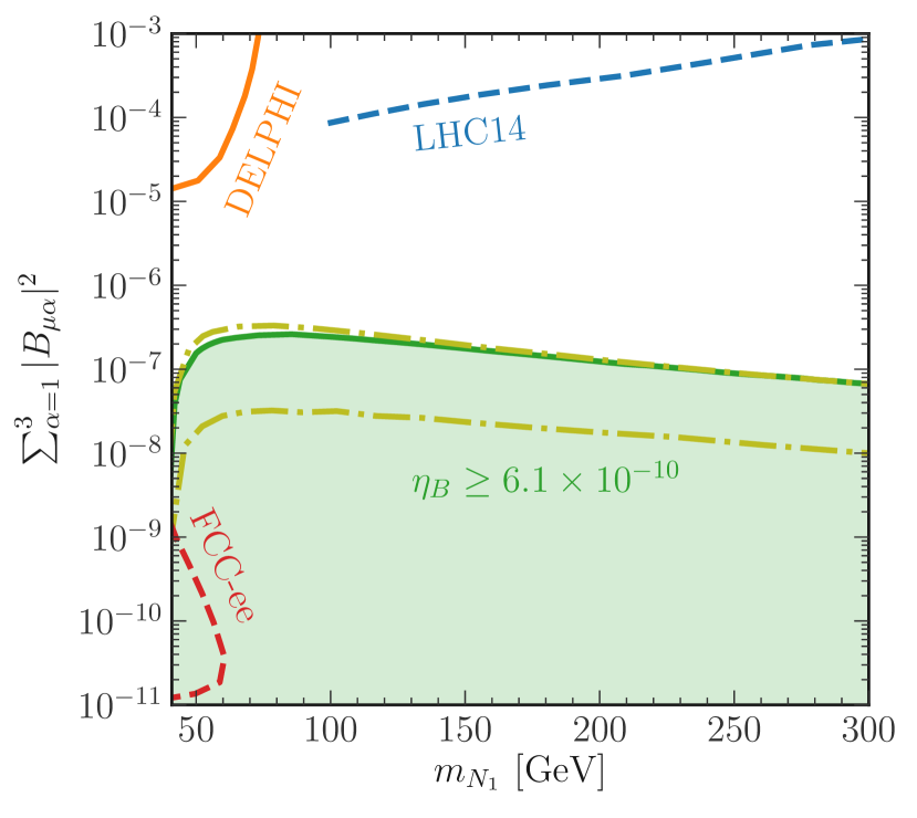
(b)

Figure 10: Parameter space for the TRL model, including current limits (solid lines) and projected sensitivities of future experiments (dashed lines). Left panel: Projected sensitivities of cLFV searches for $\mu\rightarrow e\gamma$ (orange dashed line), $\mu\rightarrow eee$ (dashed red line), coherent $\mu\rightarrow e$ conversion in titanium (dashed blue line), and current limits from searches for coherent $\mu\rightarrow e$ conversion in gold (solid blue line). These curves are based on the limits presented in (3.8) and (3.9). Right panel: Projected sensitivities for collider searches at LHC$14$ (blue dashed line), FCC-ee (red dashed line), and current limits from DELPHI (orange solid line). For details, see text. In both panels, the green region indicates points in the parameter space where leptogenesis can lead to the observed value for the baryon asymmetry, where the green solid line corresponds to the points that reproduce exactly the observed value for a tri-resonant model. The upper and lower yellow dot-dashed lines were obtained by scaling the total CP asymmetry $\delta_{T}$ by a factor of 2 and 0.1 respectively, and matching the observed baryon asymmetry. They represent an estimate of the uncertainty on the calculation of the solid green line due to oscillations.

Figure 10 shows the parameter space for the TRL model on the $\sum_{\alpha}B_{l\alpha}B^{*}_{k\alpha}$ vs. $m_{N_{1}}$ plane. For this figure, we set $a=b=c$ in (2.10). Additionally, we assume that the masses are in consecutive resonance, as defined in (4.11). For definiteness, we take as initial conditions $\eta_{L}(z_{0})=0$ and $\delta\eta_{N_{\alpha}}(z_{0})=0$, with $z_{0}=10^{-2}$, although our results are largely independent of the initial conditions. The region of parameter space that leads to a successful generation of the baryon asymmetry is depicted in green, where the solid green line indicates the value for which the obtained baryon asymmetry is equal to the observed value of $\eta^{\rm CMB}_{B}=6.104\times 10^{-10}$. The green dashed line indicates an estimate of this curve when an additional source of CP violation, generated by heavy neutrino oscillations, is included. For a fixed mass, the green region below the line yields, in principle, a higher value for $\eta_{B}$, but a relaxation of the tri-resonant condition (i.e. an increase or decrease in mass differences) can adjust the precise observed value.

In Figure 10, we have included an upper and a lower yellow dot-dashed line, obtained by scaling the total CP asymmetry $\delta_{T}$ by a factor of 2 and 0.1, respectively. They represent an estimate of the theoretical uncertainties associated to the heavy neutrino oscillation effects that were ignored in the BEs (4.19) and (4.20). This estimate was made by assuming, in line with [81], that the contribution from oscillations denoted there by $\delta\eta_{L,{\rm osc}}$ acts as a source of CP asymmetry which is distinct from and additive to the one that originates from mixing, $\delta\eta_{L,{\rm mix}}$, which we only consider here. It is necessary to point out, however, that a full three neutrino oscillation formula will differ from the approximate expression for $\delta\eta_{L,{\rm osc}}$ as presented in [81] [c.f. (5.21) therein], potentially allowing for constructive or destructive contributions to CP violating effects in the tri-resonant regime. This different treatment reflects the lack of consensus in the literature concerning whether the mixing of heavy neutrinos is contained within the oscillation phenomenon (e.g. [89]), or are two different mechanisms [81, 83]. Likewise, mixing and oscillation effects could potentially interfere, a conclusion that is supported by the results presented in [84]. On the basis of this ongoing debate, we relegate the study of tri-resonant heavy neutrino oscillation effects to a future work.

The left panel (Figure 10(a)) shows the sensitivity estimates and limits on Majorana neutrino models from searches for cLFV transitions involving muons. We only include the lines that lie close to the parameter space that leads to sufficient baryogenesis, and ignore current limits besides the one from coherent $\mu\rightarrow e$ conversion in gold. As it can be seen, the green area is currently far from the region of cLFV detection, and the only experiment that could probe this parameter space in the future is PRISM by searching for coherent $\mu\rightarrow e$ conversion in titanium. The right panel (Figure 10(b)) shows projected and current limits from collider observables. The estimate denoted by LHC$14$ (blue dashed line) presents conservative projections for the sensitivity to the process $pp\rightarrow N\ell^{\pm}jj$ at the LHC with $300~{}{\rm fb}^{-1}$ data operating at $\sqrt{s}=14~{}{\rm TeV}$ [90, 91]. The DELPHI line (orange, solid) represents 95% C.L. limits found by comparing LEP data with the prediction for signals of decaying heavy neutrinos that are produced via $Z\rightarrow N\nu_{L}$ [92]. Similar limits have been derived by the L3 collaboration [93]. The red dashed line shows the sensitivity to the same signals at the Future Circular Collider (FCC) for electron-positron collisions assuming normal order of the light neutrino spectrum, and considering the lifetime of the heavy neutrinos [94].

In summary, Figure 10(a) highlights the potential of PRISM to probe the parameter space of our leptogenesis model in the mass range below $400~{}{\rm GeV}$. On the collider front, Figure 10(b) shows that high luminosity $Z$-factories could probe the parameter space in a narrow range of masses, but for remarkably low values of the light-to-heavy neutrino mixings. Below the mass range we analyse, an extensive portion of the parameter space is ruled out by searches for heavy neutrinos that are produced in fixed target experimental facilities (e.g [95, 96, 97, 98, 99, 100, 101, 102, 103, 104]) or in atmospheric showers [105, 106, 107], while future upgrades promise a significant gain in sensitivity for the heavy neutrino parameter space. This further motivates a complete analysis including heavy neutrino oscillation effects, which could reveal a viable parameter space within the reach of these experiments. Above the $Z$ pole, the LHC $14$ projection lies far above the region where leptogenesis is successful. In models with two singlet neutrinos, an analysis searching for LNV lepton-trijet and dilepton-dijet signatures in future electron-positron, proton-proton, or electron-proton colliders shows that a sensitivity close to $10^{-6}$ could be achieved in the range of a few hundred ${\rm GeV}$ [108]. However, this is still an order of magnitude above our prediction for the viable leptogenesis parameter space, and a potential improvement on the sensitivity by the addition of a third singlet neutrino would require a dedicated analysis. A recent extensive review of current bounds and projections, including several exclusion lines that we omit in the presentation of our results, can be found in [109]. For bounds and projections on multi-TeV heavy neutrinos, the interested reader may consult the recent results communicated in [110].

7 Conclusions

We have studied a class of leptogenesis models where the smallness of the light-neutrino masses is accounted for by approximate discrete symmetries, such as $\mathbb{Z}_{3}$ or $\mathbb{Z}_{6}$ symmetries. The new feature of this class of models is that they may naturally give rise to three nearly degenerate heavy Majorana neutrinos that can strongly mix with one another and have mass differences comparable to their decay widths. In particular, we have shown how such tri-resonant heavy neutrino systems can lead to leptonic CP asymmetries that are further enhanced than those obtained in the frequently considered bi-resonant approximation. In this context, this enhanced mechanism of leptogenesis was termed Tri-Resonant Leptogenesis.

Following [16], we have formulated the BEs for TRL by considering chemical potential corrections, as well as by keeping the temperature dependence of the effective relativistic dofs of the plasma ($h_{\rm eff}$ and $g_{\rm eff}$). We have found that the latter may result in significant corrections to the heavy neutrino number density and lepton asymmetry BEs. To the best of our knowledge, these corrections have not been taken into account before in the numerical estimates of the baryon-to-photon ratio $\eta_{B}$ in thermal leptogenesis.

After performing a careful numerical study of the solutions to the evolution equations, we have explicitly demonstrated that for $m_{N}\stackrel{{\scriptstyle<}}{{{}_{\sim}}}100~{}{\rm GeV}$, the effect of the derivative of $h_{\rm eff}(T)$ with respect to the temperature $T$ of the plasma has an important influence on the evolution of the baryon asymmetry $\eta_{B}$ in the Universe. Moreover, an accurate determination of $h_{\rm eff}(T)$ will reduce the uncertainty in the predictions for the BAU. In addition, as illustrated in Figure 10, our approach to the BEs may be limited due to the uncertainties pertaining the omission of heavy neutrino oscillations, and a complete treatment would need to account for these phenomena. Given the alternate approaches to the treatment of neutrino oscillation and mixing effects, we have decided to postpone such considerations for later work.

In the TRL models that we have been studying here, the allowed parameter space that leads to successful leptogenesis gets significantly enlarged as compared to the expectation from ordinary seesaw models. Furthermore, a part of this parameter space will be probed by several projected experiments that include both cLFV and collider observables. Extensions to this model, via its supersymmetrisation, could lead to a considerable expansion of the leptogenesis parameter space due to the potential occurrence of additional cancellations that allow higher values of light-to-heavy neutrino mixings [111]. Likewise, the possible existence of more than three nearly degenerate heavy neutrinos can trigger a much more involved multi-resonant dynamics. Hence, requiring successful multi-Resonant Leptogenesis may imply a further relaxation of the stringent constraints on the theoretical parameters of such models. Finally, the inclusion of flavour effects may enhance the prospects of observable cLFV and LNV in future experiments. We aim to return and study some of the issues mentioned above in the near future.

Acknowledgements

The work of AP and DK is supported in part by the Lancaster-Manchester-Sheffield Consortium for Fundamental Physics, under STFC Research Grant ST/T001038/1. The work of PCdS is funded by Agencia Nacional de Investigación y Desarrollo (ANID) through the Becas Chile Scholarship No. 72190359. TM acknowledges support from the STFC Doctoral Training Partnership under STFC training grant ST/V506898/1.

Appendix

Appendix A Impact of $T$-dependent $h_{\rm eff}$ on BEs

In order to derive (4.19) and (4.20), we begin by writing down the general form of a BE in an isotropically expanding FRW Universe,

$$\dfrac{dn}{dt}\>+\>3\,H\,n\ =\ {\cal C}\;,$$ (A.1)

with ${\cal C}$ representing the relevant collision terms. In order to be able to solve such an equation, we rewrite it in terms of the temperature $T$, instead of the cosmic time $t$. This can be done by assuming conservation of the comoving entropy $(S=sa^{3})$, which implies $ds/dt=-3\,H\,s$. The latter observation enables us to perform the change of variables

$$\dfrac{d}{dt}=\dfrac{ds}{dt}\dfrac{dT}{ds}\dfrac{d}{dT}=H\,\delta_{h}^{-1}\dfrac{d}{d\ln z}\;,$$ (A.2)

where $\delta_{h}$ was defined in (4.18), $z=M/T$, and $M$ is some convenient mass scale, which in (4.19) and (4.20) is chosen to be $m_{N_{\alpha}}$.

For the BE that describes the evolution of the lepton asymmetry (4.20), we write the LHS of (A.1) as

$$\dfrac{dn_{L}}{dt}+3\,H\,n_{L}\,=\,\eta_{L}\,\dfrac{n_{\gamma}}{dt}+\dfrac{\eta_{L}}{dt}\,n_{\gamma}+3\,H\,\eta_{L}\,n_{\gamma}\,=\,n_{\gamma}\,H\,\delta_{h}^{-1}\bigg{[}\dfrac{d\eta_{L}}{d\ln z}+3\eta_{L}\Big{(}\delta_{h}-1\Big{)}\bigg{]}\;,$$ (A.3)

where we have used (A.2) and $dn_{\gamma}/dt=-3\,H\,\delta_{h}^{-1}\,n_{\gamma}$. Identifying ${\cal C}$ with the collision terms given in [16], we obtain the evolution equation for the lepton asymmetry (4.20).

Following the same steps as above, the heavy neutrino BE (4.19) becomes

$$\dfrac{dn_{N_{\alpha}}}{dt}+3\,H\,n_{N_{\alpha}}\,=\,n_{\gamma}\,H\,\delta_{h}^{-1}\bigg{[}\dfrac{d\eta_{N_{\alpha}}}{d\ln z}+3\eta_{N_{\alpha}}\Big{(}\delta_{h}-1\Big{)}\bigg{]}\;.$$ (A.4)

We can then express (A.4) in terms of $\delta\eta_{N_{\alpha}}$ as

$$\dfrac{dn_{N_{\alpha}}}{dt}+3\,H\,n_{N_{\alpha}}\,=\,H\,\delta_{h}^{-1}\,n_{\gamma}\,\eta_{N_{\alpha}}^{\rm eq}\bigg{[}\dfrac{d\delta\eta_{N_{\alpha}}}{d\ln z}+\Big{(}\delta\eta_{N_{\alpha}}+1\Big{)}\dfrac{d\ln\eta_{N_{\alpha}}^{\rm eq}}{d\ln z}+3\Big{(}\delta\eta_{N_{\alpha}}+1\Big{)}\Big{(}\delta_{h}-1\Big{)}\bigg{]}\;,$$ (A.5)

where

$$\dfrac{d\ln\eta_{N_{\alpha}}^{\rm eq}}{d\ln z}\,=\,-\dfrac{m_{N_{\alpha}}}{T}\dfrac{K_{1}(z_{\alpha})}{K_{2}(z_{\alpha})}\;.$$ (A.6)

Once again, substituting ${\cal C}$ for the collision terms evaluated in [16], we arrive at (4.19).

Appendix B Form Factors for cLFV Processes

We list the form factors that appear in the calculation of the cLFV processes in (3.4), (3.5) and (3.6). These depend on the light-to-heavy neutrino mixing defined in (2.5) and are given by [34, 112]

$$G_{\gamma}^{\mu e} = \sum^{3}_{\alpha=1}B_{e\alpha}B^{*}_{\mu\alpha}G_{\gamma}(x_{N_{\alpha}}),$$ (B.1)

$$F_{\gamma}^{\mu e} = \sum^{3}_{\alpha=1}B_{e\alpha}B^{*}_{\mu\alpha}F_{\gamma}(x_{N_{\alpha}}),$$ (B.2)

$$F_{Z}^{\mu e} = \sum^{3}_{\alpha=1}B_{e\alpha}B^{*}_{\mu\alpha}\left[F_{Z}(x_{N_{\alpha}})+2G_{Z}(x_{N_{\alpha}},0)\right],$$ (B.3)

$$F_{\rm Box}^{\mu euu} = \sum^{3}_{\alpha=1}B_{e\alpha}B^{*}_{\mu\alpha}\left[H_{\rm Box}(x_{N_{\alpha}},0)-H_{\rm Box}(0,0)\right],$$ (B.4)

$$F_{\rm Box}^{\mu edd} = -\sum^{3}_{\alpha=1}B_{e\alpha}B^{*}_{\mu\alpha}\left[F_{\rm Box}(x_{N_{\alpha}},0)-F_{\rm Box}(0,0)\right],$$ (B.5)

$$F_{\rm Box}^{\mu eee} = 2\>\sum^{3}_{\alpha=1}B_{e\alpha}B^{*}_{\mu\alpha}\left[F_{\rm Box}(x_{N_{\alpha}},0)-F_{\rm Box}(0,0)\right],$$ (B.6)

where $x_{N_{\alpha}}\equiv(m_{N_{\alpha}}/M_{W})^{2}$. In (B.3) and (B.6), we neglected terms of order higher than two in the light-heavy neutrino mixing parameters, since they do not modify our numerical results, while in (B.5) and (B.4) we ignore the squared modulus of non-diagonal entries of the CKM matrix.

The analytic forms of the loop functions that appear in the previous form factors are specified below:

$$G_{\gamma}(x) =-\frac{x(2x^{2}+5x-1)}{4(1-x)^{3}}-\frac{3x^{3}}{2(1-x)^{4}}\ln x,$$ (B.7)

$$F_{\gamma}(x) =\frac{x(7x^{2}-x-12)}{12(1-x)^{3}}\;-\;\frac{x^{2}(x^{2}-10x+12)}{6(1-x)^{4}}\ln x,$$ (B.8)

$$F_{Z}(x) =-\frac{5x}{2(1-x)}-\frac{5x^{2}}{2(1-x)^{2}}\ln x,$$ (B.9)

$$G_{Z}(x,0) =-\frac{x}{2(1-x)}\ln x,$$ (B.10)

$$H_{\rm Box}(x,0) =\frac{4}{1-x}+\frac{4x}{(1-x)^{2}}\ln x,$$ (B.11)

$$F_{\rm Box}(x,0) =\frac{1}{1-x}+\frac{x}{(1-x)^{2}}\ln x,$$ (B.12)

where it is helpful to indicate the limiting values $H_{\rm Box}(0,0)=4$ and $F_{\rm Box}(0,0)=1$.

Appendix C Benchmark Scenarios

For each one of the selected benchmarks presented, it is possible to find numerical solutions for the entries of perturbation matrix $\delta{\bf h}^{\nu}$ such that the model is in agreement with the observed neutrino oscillation parameters (see (3.3)). Here, we present the values of $\delta{\bf h}^{\nu}$ for four representative points, including the ones used in the evolution plots shown in Section 6.

1. $m_{N_{1}}=500~{}{\rm GeV}$, $|({\bf h}^{\nu}_{0})_{ij}|=3\times 10^{-3}$,

   $$\delta\mathbf{h}^{\nu}=\left(\begin{matrix}0&(6.40-8.15\,i)\times 10^{-12}&0\\ (-7.24+3.80\,i)\times 10^{-7}&0&-(6.91+4.37\,i)\times 10^{-7}\\ -(1.97+0.0837\,i)\times 10^{-4}&(0.911-1.75\,i)\times 10^{-4}&(1.06-1.66\,i)\times 10^{-4}\end{matrix}\right).$$

2. $m_{N_{1}}=700~{}{\rm GeV}$, $|({\bf h}^{\nu}_{0})_{ij}|=3\times 10^{-4}$,

   $$\delta\mathbf{h}^{\nu}=\left(\begin{matrix}0&(0.898-1.14\,i)\times 10^{-10}&0\\ (-8.58+4.50\,i)\times 10^{-7}&0&-(8.19+5.18\,i)\times 10^{-7}\\ -(2.02+0.0578\,i)\times 10^{-5}&(0.910-1.75\,i)\times 10^{-5}&(1.01-1.69\,i)\times 10^{-5}\end{matrix}\right).$$

3. $m_{N_{1}}=1~{}{\rm TeV}$, $|({\bf h}^{\nu}_{0})_{ij}|=3\times 10^{-4}$,

   $$\delta\mathbf{h}^{\nu}=\left(\begin{matrix}0&(1.29-1.64\,i)\times 10^{-10}&0\\ (-1.03+0.539\,i)\times 10^{-6}&0&-(9.80+6.20\,i)\times 10^{-7}\\ -(2.03+5.19\,i)\times 10^{-5}&(0.910-1.75\,i)\times 10^{-5}&(1.00-1.70\,i)\times 10^{-5}\end{matrix}\right).$$

4. $m_{N_{1}}=120~{}{\rm GeV}$, $|({\bf h}^{\nu}_{0})_{ij}|=2\times 10^{-4}$,

   $$\delta\mathbf{h}^{\nu}=\left(\begin{matrix}0&(2.46-3.14\,i)\times 10^{-11}&0\\ (-3.53+1.85\,i)\times 10^{-7}&0&-(3.37+2.13\,i)\times 10^{-7}\\ -(1.24+0.0421\,i)\times 10^{-5}&-(0.562+1.08\,i)\times 10^{-5}&(0.637-1.04\,i)\times 10^{-5}\end{matrix}\right).$$

We note that for all the benchmark models listed above, we have $m_{N_{1}}\approx m_{N_{2}}\approx m_{N_{3}}$, such that their mass differences are subleading to the light-neutrino masses and their mixing.

References

- [1] Planck Collaboration, N. Aghanim et al., Planck 2018 results. VI. Cosmological parameters, Astron. Astrophys. 641 (2020) A6, [arXiv:1807.06209]. [Erratum: Astron.Astrophys. 652, C4 (2021)].
- [2] B. D. Fields, K. A. Olive, T.-H. Yeh, and C. Young, Big-Bang Nucleosynthesis after Planck, JCAP 03 (2020) 010, [arXiv:1912.01132]. [Erratum: JCAP 11, E02 (2020)].
- [3] SNO Collaboration, Q. R. Ahmad et al., Measurement of the rate of interactions produced by solar neutrinos at the Sudbury Neutrino Observatory, Phys. Rev. Lett. 87 (2001) 071301, [nucl-ex/0106015].
- [4] SNO Collaboration, Q. R. Ahmad et al., Direct evidence for neutrino flavor transformation from neutral current interactions in the Sudbury Neutrino Observatory, Phys. Rev. Lett. 89 (2002) 011301, [nucl-ex/0204008].
- [5] Super-Kamiokande Collaboration, Y. Fukuda et al., Evidence for oscillation of atmospheric neutrinos, Phys. Rev. Lett. 81 (1998) 1562–1567, [hep-ex/9807003].
- [6] P. Minkowski, at a Rate of One Out of Muon Decays?, Phys. Lett. 67B (1977) 421–428.
- [7] M. Gell-Mann, P. Ramond, and R. Slansky, Complex Spinors and Unified Theories, Conf. Proc. C790927 (1979) 315–321, [arXiv:1306.4669].
- [8] T. Yanagida, Horizontal gauge symmetry and masses of neutrinos, Conf. Proc. C7902131 (1979) 95–99.
- [9] R. N. Mohapatra and G. Senjanovic, Neutrino Mass and Spontaneous Parity Nonconservation, Phys. Rev. Lett. 44 (1980) 912.
- [10] A. D. Sakharov, Violation of CP Invariance, C asymmetry, and baryon asymmetry of the universe, Pisma Zh. Eksp. Teor. Fiz. 5 (1967) 32–35.
- [11] M. Fukugita and T. Yanagida, Baryogenesis without grand unification, Phys. Lett. B174 (1986) 45.
- [12] A. Pilaftsis, CP violation and baryogenesis due to heavy Majorana neutrinos, Phys. Rev. D 56 (1997) 5431–5451, [hep-ph/9707235].
- [13] A. Pilaftsis and T. E. J. Underwood, Resonant leptogenesis, Nucl. Phys. B 692 (2004) 303–345, [hep-ph/0309342].
- [14] P. Di Bari and R. Samanta, The -inspired leptogenesis timely opportunity, JHEP 08 (2020) 124, [arXiv:2005.03057].
- [15] A. Pilaftsis, Heavy Majorana neutrinos and baryogenesis, Int. J. Mod. Phys. A 14 (1999) 1811–1858, [hep-ph/9812256].
- [16] A. Pilaftsis and T. E. J. Underwood, Electroweak-scale resonant leptogenesis, Phys. Rev. D 72 (2005) 113001, [hep-ph/0506107].
- [17] A. Blondel et al., Research Proposal for an Experiment to Search for the Decay , arXiv:1301.6113.
- [18] MEG Collaboration, A. M. Baldini et al., Search for the lepton flavour violating decay with the full dataset of the MEG experiment, Eur. Phys. J. C 76 (2016), no. 8 434, [arXiv:1605.05081].
- [19] MEG II Collaboration, A. M. Baldini et al., The design of the MEG II experiment, Eur. Phys. J. C 78 (2018), no. 5 380, [arXiv:1801.04688].
- [20] COMET Collaboration, M. Moritsu, Search for muon-to-electron conversion with the COMET experiment, Universe 8 (2022) 196, [arXiv:2203.06365].
- [21] R. Barlow, The PRISM/PRIME Project, Nuclear Physics B - Proceedings Supplements 218 (2011), no. 1 44–49. Proceedings of the Eleventh International Workshop on Tau Lepton Physics.
- [22] F. F. Deppisch and A. Pilaftsis, Lepton Flavour Violation and in Minimal Resonant Leptogenesis, Phys. Rev. D 83 (2011) 076007, [arXiv:1012.1834].
- [23] A. Pilaftsis and D. Teresi, Mass bounds on light and heavy neutrinos from radiative minimal-flavor-violation leptogenesis, Phys. Rev. D 92 (2015), no. 8 085016, [arXiv:1506.08124].
- [24] A. Pilaftsis, Radiatively induced neutrino masses and large Higgs neutrino couplings in the standard model with Majorana fields, Z. Phys. C 55 (1992) 275–282, [hep-ph/9901206].
- [25] P. S. B. Dev and A. Pilaftsis, Minimal Radiative Neutrino Mass Mechanism for Inverse Seesaw Models, Phys. Rev. D 86 (2012) 113001, [arXiv:1209.4051].
- [26] B. Pontecorvo, Inverse beta processes and nonconservation of lepton charge, Sov. Phys. JETP 7 (1958) 172–173.
- [27] Z. Maki, M. Nakagawa, and S. Sakata, Remarks on the unified model of elementary particles, Prog. Theor. Phys. 28 (1962) 870–880.
- [28] L. Autonne, Sur les matrices hypohermitiennes et sur les matrices unitaires, Annales De L’Université de Lyons, Nouvelle Série I 38 (1915) 1–77.
- [29] T. Takagi Japan J. Math. 1 (1925) 83.
- [30] S. Bilenky, J. Hošek, and S. Petcov, On the oscillations of neutrinos with Dirac and Majorana masses, Physics Letters B 94 (1980), no. 4 495–498.
- [31] J. Schechter and J. W. F. Valle, Neutrino Masses in SU(2) U(1) Theories, Phys. Rev. D 22 (1980) 2227.
- [32] P. de Salas, D. Forero, S. Gariazzo, P. Martínez-Miravé, O. Mena, C. Ternes, M. Tórtola, and J. Valle, 2020 Global reassessment of the neutrino oscillation picture, arXiv:2006.11237.
- [33] T. P. Cheng and L.-F. Li, in Theories With Dirac and Majorana Neutrino Mass Terms, Phys. Rev. Lett. 45 (1980) 1908.
- [34] A. Ilakovac and A. Pilaftsis, Flavor violating charged lepton decays in seesaw-type models, Nucl. Phys. B 437 (1995) 491, [hep-ph/9403398].
- [35] R. Alonso, M. Dhen, M. B. Gavela, and T. Hambye, Muon conversion to electron in nuclei in type-I seesaw models, JHEP 01 (2013) 118, [arXiv:1209.2679].
- [36] R. Kitano, M. Koike, and Y. Okada, Detailed calculation of lepton flavor violating muon electron conversion rate for various nuclei, Phys. Rev. D 66 (2002) 096002, [hep-ph/0203110]. [Erratum: Phys.Rev.D 76, 059902 (2007)].
- [37] SINDRUM Collaboration, U. Bellgardt et al., Search for the Decay , Nucl. Phys. B 299 (1988) 1–6.
- [38] SINDRUM II Collaboration, W. H. Bertl et al., A Search for muon to electron conversion in muonic gold, Eur. Phys. J. C 47 (2006) 337–346.
- [39] S. Di Falco, Status of the Mu2e experiment at Fermilab, PoS EPS-HEP2021 (2022) 557.
- [40] A. Abada, J. Kriewald, and A. M. Teixeira, On the role of leptonic CPV phases in cLFV observables, Eur. Phys. J. C 81 (2021), no. 11 1016, [arXiv:2107.06313].
- [41] J. Liu and G. Segrè, Reexamination of generation of baryon and lepton number asymmetries in the early Universe by heavy particle decay, Phys. Rev. D 48 (Nov, 1993) 4609–4612.
- [42] A. Pilaftsis, Resonant CP violation induced by particle mixing in transition amplitudes, Nucl. Phys. B 504 (1997) 61–107, [hep-ph/9702393].
- [43] G. C. Branco, L. Lavoura, and M. N. Rebelo, Majorana Neutrinos and CP Violation in the Leptonic Sector, Phys. Lett. B 180 (1986) 264–268.
- [44] B. Yu and S. Zhou, Sufficient and Necessary Conditions for CP Conservation in the Case of Degenerate Majorana Neutrino Masses, Phys. Rev. D 103 (2021), no. 3 035017, [arXiv:2009.12347].
- [45] P.-H. Gu and U. Sarkar, Leptogenesis with Linear, Inverse or Double Seesaw, Phys. Lett. B 694 (2011) 226–232, [arXiv:1007.2323].
- [46] M. Garny, A. Kartavtsev, and A. Hohenegger, Leptogenesis from first principles in the resonant regime, Annals Phys. 328 (2013) 26–63, [arXiv:1112.6428].
- [47] M. Aoki, N. Haba, and R. Takahashi, A model realizing inverse seesaw and resonant leptogenesis, PTEP 2015 (2015), no. 11 113B03, [arXiv:1506.06946].
- [48] T. Asaka and T. Yoshida, Resonant leptogenesis at TeV-scale and neutrinoless double beta decay, JHEP 09 (2019) 089, [arXiv:1812.11323].
- [49] A. Granelli, K. Moffat, and S. Petcov, Flavoured resonant leptogenesis at sub-TeV scales, Nuclear Physics B 973 (2021) 115597.
- [50] G. Chauhan and P. S. B. Dev, Resonant Leptogenesis, Collider Signals and Neutrinoless Double Beta Decay from Flavor and CP Symmetries, arXiv:2112.09710.
- [51] I. Chakraborty, H. Roy, and T. Srivastava, Resonant leptogenesis in (2,2) inverse see-saw realisation, Nuclear Physics B 979 (2022) 115780.
- [52] A. Abada, G. Arcadi, V. Domcke, M. Drewes, J. Klaric, and M. Lucente, Low-scale leptogenesis with three heavy neutrinos, JHEP 01 (2019) 164, [arXiv:1810.12463].
- [53] M. Drewes, Y. Georis, and J. Klarić, Mapping the Viable Parameter Space for Testable Leptogenesis, Phys. Rev. Lett. 128 (2022), no. 5 051801, [arXiv:2106.16226].
- [54] M. Drewes, Y. Georis, C. Hagedorn, and J. Klarić, Low-scale leptogenesis with flavour and CP symmetries, arXiv:2203.08538.
- [55] A. Granelli, J. Klarić, and S. T. Petcov, Tests of Low-Scale Leptogenesis in Charged Lepton Flavour Violation Experiments, arXiv:2206.04342.
- [56] A. Pilaftsis, Resonant tau-leptogenesis with observable lepton number violation, Phys. Rev. Lett. 95 (2005) 081602, [hep-ph/0408103].
- [57] V. Kuzmin, V. Rubakov, and M. Shaposhnikov, On anomalous electroweak baryon-number non-conservation in the early universe, Physics Letters B 155 (1985), no. 1 36–42.
- [58] G. Belanger, F. Boudjema, A. Pukhov, and A. Semenov, micrOMEGAs3: A program for calculating dark matter observables, Comput. Phys. Commun. 185 (2014) 960–985, [arXiv:1305.0237].
- [59] M. Hindmarsh and O. Philipsen, WIMP dark matter and the QCD equation of state, Phys. Rev. D 71 (2005) 087302, [hep-ph/0501232].
- [60] F. Karsch, E. Laermann, and A. Peikert, The Pressure in two flavor, (2+1)-flavor and three flavor QCD, Phys. Lett. B 478 (2000) 447–455, [hep-lat/0002003].
- [61] K. Kajantie, M. Laine, K. Rummukainen, and Y. Schroder, The Pressure of hot QCD up to g6 ln(1/g), Phys. Rev. D 67 (2003) 105008, [hep-ph/0211321].
- [62] J. Rang, Improved traditional Rosenbrock–Wanner methods for stiff ODEs and DAEs, Journal of Computational and Applied Mathematics 286 (2015) 128–144.
- [63] D. Karamitros, NaBBODES: Not a Black Box Ordinary Differential Equation Solver in C++, 2019.
- [64] P. Rentrop and P. Kaps, Generalized Runge-Kutta Methods of Order Four with Stepsize Control for Stiff Ordinary Differential Equations., Numerische Mathematik 33 (1979) 55–68.
- [65] J. Rang and L. Angermann, New Rosenbrock W-Methods of Order 3 for Partial Differential Algebraic Equations of Index 1, BIT Numerical Mathematics 45 (2005) 761–787.
- [66] P. Virtanen, R. Gommers, T. E. Oliphant, M. Haberland, T. Reddy, D. Cournapeau, E. Burovski, P. Peterson, W. Weckesser, J. Bright, S. J. van der Walt, M. Brett, J. Wilson, K. J. Millman, N. Mayorov, A. R. J. Nelson, E. Jones, R. Kern, E. Larson, C. J. Carey, İ. Polat, Y. Feng, E. W. Moore, J. VanderPlas, D. Laxalde, J. Perktold, R. Cimrman, I. Henriksen, E. A. Quintero, C. R. Harris, A. M. Archibald, A. H. Ribeiro, F. Pedregosa, P. van Mulbregt, and SciPy 1.0 Contributors, SciPy 1.0: Fundamental Algorithms for Scientific Computing in Python, Nature Methods 17 (2020) 261–272.
- [67] D. Karamitros, SimpleSplines: A header only library for linear and cubic spline interpolation in C++, 2021.
- [68] D. Karamitros, LAInt: A header only library for local adaptive integration in C++, 2022.
- [69] J. D. Hunter, Matplotlib: A 2d graphics environment, Computing in Science & Engineering 9 (2007), no. 3 90–95.
- [70] H. A. Weldon, Effective Fermion Masses of Order gT in High Temperature Gauge Theories with Exact Chiral Invariance, Phys. Rev. D 26 (1982) 2789.
- [71] M. D’Onofrio, K. Rummukainen, and A. Tranberg, Sphaleron Rate in the Minimal Standard Model, Phys. Rev. Lett. 113 (2014), no. 14 141602, [arXiv:1404.3565].
- [72] W. Buchmuller, P. Di Bari, and M. Plumacher, Leptogenesis for pedestrians, Annals Phys. 315 (2005) 305–351, [hep-ph/0401240].
- [73] J. A. Harvey and M. S. Turner, Cosmological baryon and lepton number in the presence of electroweak fermion-number violation, Phys. Rev. D 42 (Nov, 1990) 3344–3349.
- [74] P. Gondolo and G. Gelmini, Cosmic abundances of stable particles: Improved analysis, Nucl. Phys. B 360 (1991) 145–179.
- [75] E. K. Akhmedov, V. A. Rubakov, and A. Y. Smirnov, Baryogenesis via neutrino oscillations, Phys. Rev. Lett. 81 (1998) 1359–1362, [hep-ph/9803255].
- [76] T. Asaka and M. Shaposhnikov, The MSM, dark matter and baryon asymmetry of the universe, Phys. Lett. B 620 (2005) 17–26, [hep-ph/0505013].
- [77] T. Asaka, S. Eijima, and H. Ishida, Kinetic Equations for Baryogenesis via Sterile Neutrino Oscillation, JCAP 02 (2012) 021, [arXiv:1112.5565].
- [78] B. Shuve and I. Yavin, Baryogenesis through Neutrino Oscillations: A Unified Perspective, Phys. Rev. D 89 (2014), no. 7 075014, [arXiv:1401.2459].
- [79] T. Hambye and D. Teresi, Higgs doublet decay as the origin of the baryon asymmetry, Phys. Rev. Lett. 117 (2016), no. 9 091801, [arXiv:1606.00017].
- [80] M. Drewes, B. Garbrecht, D. Gueter, and J. Klaric, Leptogenesis from Oscillations of Heavy Neutrinos with Large Mixing Angles, JHEP 12 (2016) 150, [arXiv:1606.06690].
- [81] P. S. Bhupal Dev, P. Millington, A. Pilaftsis, and D. Teresi, Flavour Covariant Transport Equations: an Application to Resonant Leptogenesis, Nucl. Phys. B 886 (2014) 569–664, [arXiv:1404.1003].
- [82] J. Klarić, M. Shaposhnikov, and I. Timiryasov, Reconciling resonant leptogenesis and baryogenesis via neutrino oscillations, Phys. Rev. D 104 (2021), no. 5 055010, [arXiv:2103.16545].
- [83] P. S. Bhupal Dev, P. Millington, A. , and D. Teresi, Kadanoff–Baym approach to flavour mixing and oscillations in resonant leptogenesis, Nucl. Phys. B 891 (2015) 128–158, [arXiv:1410.6434].
- [84] A. Kartavtsev, P. Millington, and H. Vogel, Lepton asymmetry from mixing and oscillations, JHEP 06 (2016) 066, [arXiv:1601.03086].
- [85] J. Racker, CP violation in mixing and oscillations in a toy model for leptogenesis with quasi-degenerate neutrinos, JHEP 04 (2021) 290, [arXiv:2012.05354].
- [86] H. Jukkala, K. Kainulainen, and P. M. Rahkila, Flavour mixing transport theory and resonant leptogenesis, JHEP 09 (2021) 119, [arXiv:2104.03998].
- [87] J. Racker, CP violation in mixing and oscillations for leptogenesis. Part II. The highly degenerate case, JHEP 11 (2021) 027, [arXiv:2109.00040].
- [88] T. Hambye and D. Teresi, Baryogenesis from -violating Higgs-doublet decay in the density-matrix formalism, Phys. Rev. D 96 (Jul, 2017) 015031.
- [89] B. Garbrecht and M. Herranen, Effective Theory of Resonant Leptogenesis in the Closed-Time-Path Approach, Nucl. Phys. B 861 (2012) 17–52, [arXiv:1112.5954].
- [90] F. F. Deppisch, P. S. Bhupal Dev, and A. Pilaftsis, Neutrinos and Collider Physics, New J. Phys. 17 (2015), no. 7 075019, [arXiv:1502.06541].
- [91] P. S. B. Dev, A. Pilaftsis, and U. K. Yang, New Production Mechanism for Heavy Neutrinos at the LHC, Phys. Rev. Lett. 112 (2014), no. 8 081801, [arXiv:1308.2209].
- [92] DELPHI Collaboration, P. Abreu et al., Search for neutral heavy leptons produced in Z decays, Z. Phys. C 74 (1997) 57–71. [Erratum: Z.Phys.C 75, 580 (1997)].
- [93] L3 Collaboration, O. Adriani et al., Search for isosinglet neutral heavy leptons in Z0 decays, Phys. Lett. B 295 (1992) 371–382.
- [94] FCC-ee study Team Collaboration, A. Blondel, E. Graverini, N. Serra, and M. Shaposhnikov, Search for Heavy Right Handed Neutrinos at the FCC-ee, Nucl. Part. Phys. Proc. 273-275 (2016) 1883–1890, [arXiv:1411.5230].
- [95] PIENU Collaboration, A. Aguilar-Arevalo et al., Improved search for heavy neutrinos in the decay , Phys. Rev. D 97 (2018), no. 7 072012, [arXiv:1712.03275].
- [96] PIENU Collaboration, A. Aguilar-Arevalo et al., Search for heavy neutrinos in decay, Phys. Lett. B 798 (2019) 134980, [arXiv:1904.03269].
- [97] NA62 Collaboration, E. Cortina Gil et al., Search for heavy neutral lepton production in decays to positrons, Phys. Lett. B 807 (2020) 135599, [arXiv:2005.09575].
- [98] NA62 Collaboration, E. Cortina Gil et al., Search for decays to a muon and invisible particles, Phys. Lett. B 816 (2021) 136259, [arXiv:2101.12304].
- [99] G. Bernardi et al., Search for Neutrino Decay, Phys. Lett. B 166 (1986) 479–483.
- [100] G. Bernardi et al., Further limits on heavy neutrino couplings, Phys. Lett. B 203 (1988) 332–334.
- [101] NuTeV, E815 Collaboration, A. Vaitaitis et al., Search for neutral heavy leptons in a high-energy neutrino beam, Phys. Rev. Lett. 83 (1999) 4943–4946, [hep-ex/9908011].
- [102] T2K Collaboration, K. Abe et al., Search for heavy neutrinos with the T2K near detector ND280, Phys. Rev. D 100 (2019), no. 5 052006, [arXiv:1902.07598].
- [103] MicroBooNE Collaboration, P. Abratenko et al., Search for Heavy Neutral Leptons Decaying into Muon-Pion Pairs in the MicroBooNE Detector, Phys. Rev. D 101 (2020), no. 5 052001, [arXiv:1911.10545].
- [104] NOMAD Collaboration, P. Astier et al., Search for heavy neutrinos mixing with tau neutrinos, Phys. Lett. B 506 (2001) 27–38, [hep-ex/0101041].
- [105] A. Kusenko, S. Pascoli, and D. Semikoz, New bounds on MeV sterile neutrinos based on the accelerator and Super-Kamiokande results, JHEP 11 (2005) 028, [hep-ph/0405198].
- [106] P. Coloma, P. Hernández, V. Muñoz, and I. M. Shoemaker, New constraints on Heavy Neutral Leptons from Super-Kamiokande data, Eur. Phys. J. C 80 (2020), no. 3 235, [arXiv:1911.09129].
- [107] C. Argüelles, P. Coloma, P. Hernández, and V. Muñoz, Searches for Atmospheric Long-Lived Particles, JHEP 02 (2020) 190, [arXiv:1910.12839].
- [108] S. Antusch, E. Cazzato, and O. Fischer, Sterile neutrino searches at future , , and colliders, Int. J. Mod. Phys. A 32 (2017), no. 14 1750078, [arXiv:1612.02728].
- [109] A. M. Abdullahi et al., The Present and Future Status of Heavy Neutral Leptons, in 2022 Snowmass Summer Study, 3, 2022. arXiv:2203.08039.
- [110] K. A. U. Calderón, I. Timiryasov, and O. Ruchayskiy, Improved constraints and the prospects of detecting TeV to PeV scale Heavy Neutral Leptons, arXiv:2206.04540.
- [111] P. Candia da Silva and A. Pilaftsis, Radiative neutrino masses in the MSSM, Phys. Rev. D 102 (2020), no. 9 095013, [arXiv:2008.05450].
- [112] A. Ilakovac, B. A. Kniehl, and A. Pilaftsis, Semileptonic lepton number / flavor violating tau decays in Majorana neutrino models, Phys. Rev. D 52 (1995) 3993–4005, [hep-ph/9503456].
- [113] A. Meurer, C. P. Smith, M. Paprocki, O. Čertík, S. B. Kirpichev, M. Rocklin, A. Kumar, S. Ivanov, J. K. Moore, S. Singh, T. Rathnayake, S. Vig, B. E. Granger, R. P. Muller, F. Bonazzi, H. Gupta, S. Vats, F. Johansson, F. Pedregosa, M. J. Curry, A. R. Terrel, v. Roučka, A. Saboo, I. Fernando, S. Kulal, R. Cimrman, and A. Scopatz, SymPy: symbolic computing in Python, PeerJ Computer Science 3 (Jan., 2017) e103.