Pythae: Unifying Generative Autoencoders in Python A Benchmarking Use Case

Abstract

In recent years, deep generative models have attracted increasing interest due to their capacity to model complex distributions. Among those models, variational autoencoders have gained popularity as they have proven both to be computationally efficient and yield impressive results in multiple fields. Following this breakthrough, extensive research has been done in order to improve the original publication, resulting in a variety of different VAE models in response to different tasks. In this paper we present Pythae, a versatile open-source Python library providing both a unified implementation and a dedicated framework allowing straightforward, reproducible and reliable use of generative autoencoder models. As an example of application, we propose to use this library to perform a case study benchmark where we present and compare 19 generative autoencoder models representative of some of the main improvements on downstream tasks such as image reconstruction, generation, classification, clustering and interpolation. The open-source library can be found at https://github.com/clementchadebec/benchmark_VAE.

1 Introduction

Over the past few years, generative models have proven to be a promising approach for modelling datasets with complex inherent distributions such a natural images. Among those, Variational AutoEncoders (VAE) [37, 56] have gained popularity due to their computational efficiency and scalability, leading to many applications such as speech modelling [10], clustering [24, 70], data augmentation [14] or image generation [54]. Similarly to autoencoders, these models encourage good reconstruction of an observed input data from a latent representation, but they further assume latent vectors to be random variables involved in the generation process of the observed data. This imposes a latent structure wherein latent variables are driven to follow a prior distribution that can then be used to generate new data. Since this breakthrough, various contributions have been made to enrich the original VAE scheme through new generating strategies [24, 65, 27, 5, 50], reconstruction objectives [41, 61] and more adapted latent representations [30, 35, 66, 3, 14] to cite a few. A drawback of VAEs is that due to the intractability of the log-likelihood objective function, VAEs have to resort to optimizing a lower bound on the true objective as a proxy, which has been mentionned as a major limitation of the model [11, 1, 30, 21, 71]. Hence, extensive research has been proposed to improve this bound through richer distributions [57, 55, 38, 13]. More recently, it has been shown that autoencoders can be turned into generative approaches through latent density estimation [27], extending the concept of Generative AutoEncoders (GAE) to a more general class of autoencoder models.

Nonetheless, most of this research has been done in parallel across disjoint sub-fields of research and to the best of our knowledge little to no work has been done on homogenising and integrating these distinct methods in a common framework. Moreover, for many of the aforementioned publications, implementations may not be available or maintained, therefore requiring time-consuming re-implementation. This induces a strong bottleneck for research to move forward in this field and makes reproducibility challenging, which calls for the need of a unified generative autoencoder framework. To address this issue we introduce Pythae (Python AutoEncoder), a versatile open source Python library for generative autoencoders providing unified implementations of common methods, along with a reproducible framework allowing for easy model training, data generation and experiment tracking. We then propose to illustrate the usefulness of the proposed library on a benchmark case study of 19 generative autoencoder methods on classical image datasets. We consider five different downstream tasks: image reconstruction and generation, latent vector classification and clustering, and image interpolation on three well known imaging datasets.

2 Variational autoencoders

In this section, we recall the original VAE setting and present some of the main improvements that were proposed to enhance the model.

2.1 Background

Given $x\in\mathbb{R}^{D}$, a set of observed variables deriving from an unknown distribution $p(x)$, a VAE assumes that there exists $z\in\mathbb{R}^{d}$ such that $z$ is a latent representation of $x$. The generation process of $x$ thus decomposes as

$$p_{\theta}(x)=\int_{\mathcal{Z}}p_{\theta}(x|z)p_{z}(z)dz\,,$$ (1)

where $p_{z}$ is the prior distribution on the latent space $\mathbb{R}^{d}$. The distribution $p_{\theta}(x|z)$ is referred to as the decoder and is modelled with a simple parametric distribution whose parameters are given by a neural network. Since the true posterior $p_{\theta}(z|x)$ is most of the time intractable due to the integral in Eq. (1) recourse to Variational Inference [32] is needed and a variational distribution $q_{\phi}(z|x)$ which we refer to as the encoder is introduced. The approximate posterior $q_{\phi}$ is again taken as a simple parametric distribution whose parameters are also modelled by a neural network. This allows to define an unbiased estimate $\widehat{p}_{\theta}$ of the marginal distribution $p_{\theta}(x)$ using importance sampling with $q_{\phi}(z|x)$ i.e. $\widehat{p}_{\theta}(x)=\frac{p_{\theta}(x|z)p_{z}(z)}{q_{\phi}(z|x)}$ and $\mathbb{E}_{z\sim q_{\phi}}\big{[}\widehat{p}_{\theta}\big{]}=p_{\theta}$. Applying Jensen’s inequality leads to a lower bound on the likelihood given in Eq. (1):

$$\log\underbrace{\mathbb{E}_{z\sim q_{\phi}}\big{[}\widehat{p}_{\theta}(x)\big{]}}_{p_{\theta}(x)} \geq\mathbb{E}_{z\sim q_{\phi}}\big{[}\log\widehat{p}_{\theta}(x)\big{]}=\underbrace{\mathbb{E}_{z\sim q_{\phi}}[\log p_{\theta}(x|z)]}_{\text{reconstruction}}-\underbrace{\mathcal{D}_{KL}\big{[}q_{\phi}(z|x)||p_{z}(z)\big{]}}_{\text{regularisation}}\,,$$ (2)

where $\mathcal{D}_{KL}(p||q)$ is the Kullback-Leibler divergence between distributions $p$ and $q$. This bound is referred to as the Evidence Lower Bound (ELBO) [37] and is used as the training objective to maximize in the traditional VAE scheme. It can be interpreted as a two terms objective [27] where the reconstruction loss forces the output of the decoder to be close to the original input $x$, while the regularisation loss forces the posterior distribution $q_{\phi}(z|x)$ outputted by the encoder to be close to the prior distribution $p_{z}(z)$. Under standard VAE assumption, the prior distribution is a multivariate standard Gaussian $p_{z}=\mathcal{N}(0,I_{d})$, the approximate posterior is set to $q_{\phi}(z|x)=\mathcal{N}\big{(}z\big{|}\mu(x),\Sigma(x)\big{)}$ where $\big{(}\mu(x),\Sigma(x)\big{)}$ are outputs of the encoder network.

2.2 Improvements upon the classical VAE method

Building on the breakthrough of VAEs, several papers have proposed improvements to the model. In this section we present 4 axes which we consider to be representative of the major advancements made on VAEs, as well as classical models characterising the main improvements within each of these axes.

Improving the prior

It has been shown that the role of the prior distribution $p_{z}$ is crucial in the good performance of the VAE [31] and choosing a family of overly simplistic priors can lead to over-regularization [20] and poor reconstruction performance [22]. In particular, it was shown that the prior maximizing the ELBO objective is the aggregated posterior $q(z)=\frac{1}{N}\sum_{i=1}^{N}q_{\phi}(z|x_{i})$ [65]. However, it should be noted that a perfect fit between the prior and the aggregated posterior is not necessarily desired since it has been shown in [6, 65] that it may lead to over-fitting as it essentially amounts to the model memorising the training set. Hence, multi-modal priors [48, 24, 65] were proposed, followed by hierarchical latent variable models [62, 39] and prior learning based approaches [17, 2] to address the poor expressiveness of the prior distribution and model richer generative distributions. Considering a specific geometry of the latent space also led to alternative priors taking into account geometrical aspects of the latent space [23, 25, 45, 3, 15, 59, 34, 14]. Another interesting approach proposed for instance in [66, 27] consists in using density estimation post training with another distribution or normalising flows [55] on the learned latent codes.

Towards a better lower bound Another major axis of improvement of the VAE model has been to tighten the gap between the ELBO objective and the true log probability [11, 1, 30, 21, 71]. The ELBO objective can indeed be written as the difference between the true log probability and a KL divergence between the approximate posterior and the true posterior

$$\mathcal{L}_{\text{ELBO}}(x)=\log p_{\theta}(x)-\mathcal{D}_{KL}\big{[}q_{\phi}(z|x)||p(z|x)\big{]}\,.$$ (3)

Hence, if one wants to make the ELBO gap tighter, particular attention should be paid to the choice in the approximate posterior $q_{\phi}(z|x)$. In the original model, $q_{\phi}(z|x)$ is chosen as a simple distribution for tractability of the ELBO in Eq. (2). However, several approaches have been proposed to extend the choice of $q_{\phi}$ to a wider class of distributions using MCMC sampling [57] or normalising flows [55]. For instance, Kingma et al. [38] improve upon the works of [55] with an inverse auto-regressive normalising flow (IAF), a new type of normalizing flow that better scales to high-dimensional latent spaces. With this objective in mind a Hamiltonian VAE aimed at targeting the true posterior during training with a Hamiltonian Monte Carlo [49] inspired scheme was proposed [13] and extended to Riemannian latent spaces in [14].

Encouraging disentanglement

Although there is no clear consensus upon the definition of disentanglement, it is commonly referred to as the independence between features in a representation [46]. This is a desirable behaviour for VAEs, as it is argued that disentangled features may be more representative and interpretable [30]. In that regard, several approaches have been proposed encouraging a better disentanglement of the features in the latent space. Higgins et al. [30] first argue that increasing the weight of the KL divergence term in the ELBO loss enforces a higher disentanglement of the latent features as the posterior probability is forced to match a multivariate normal standard Gaussian. Following this idea, [12] propose to achieve disentanglement by gradually increasing the proximity between the posterior and the prior [12]. Other methods challenge the view that disentanglement can be achieved by simply forcing the posterior to match the prior, or raise the point that in this case disentanglement is achieved at the cost of a bad reconstruction. From these observations, new approaches arise such as [35] who augment the VAE objective with a penalty that encourages factorial representation of the marginal distributions, or [16] that enforce a penalty on the total correlation favouring disentanglement.

Amending the distance between distributions It can be stressed that the reconstruction term $\mathbb{E}_{z\sim q_{\phi}(z|x)}[\log p_{\theta}(x|z)]$ in eq. (2) has a crucial role in the reconstruction and that its choice should be dependent of the application. For instance, methods using a discriminator [41] or using a deterministic differentiable loss function [61] acting as a distance between the input data and its reconstruction were also proposed. The second term in the ELBO measures the distance between the approximate posterior and the prior distribution through the KL divergence and it has however been argued that other distances between probability distributions could be used instead. Hence, approaches using a GAN to distinguish samples from the posterior from samples from the prior distribution [44] or methods based on optimal transport have also been proposed [64, 72].

3 The Pythae library

Why Pythae ?

To the best of our knowledge, although some well referenced libraries grouping different Variational Auto-Encoder methods exist (e.g. [63]), there exists no framework providing both adaptable and easy-to-use unified implementations of state-of-the-art Generative AutoEncoder (GAE) methods. This induces both a strong brake for reproducible research and democratisation of the models since implementations might be difficult to adapt to other use-cases, no longer maintained, or completely unavailable.

Project vision

Starting from this observation, we created Pythae, an open-source python library inspired from [53, 69] providing unified implementations of generative autoencoding methods, allowing for easy use and training of GAE models. Pythae is designed with the following points in mind:

• Usable by all Pythae makes GAE models accessible to all - beginners to experts. This means beginners can run ready-to-use models with a few lines of code, while more advanced users can easily access and adapt different methods to their specific use-cases, with custom encoder/decoder definition. Indeed, the library was designed to be flexible enough to allow users to use existing implementations on their own data, with custom model hyper-parameters, training configurations and network architectures.

  The library has an online documentation and is also explained and illustrated through tutorials available either on a local machine or on the Google Colab platform [9].

• Unified implementation The brick-like structure of Pythae allows for seamless but efficient interchange between models, sampling techniques, network architectures, model hyper-parameters and training schemes. Pythae is unit-tested ensuring code quality and continuous development with a code coverage of 98% as of release 0.6. The library is made available on pip and conda allowing an easy integration. Its development is performed through releases that ensure stable and robust implementations.

• A reproducible research environment Pythae is open to all and as such encourages transparent and reproducible research, as illustrated in the next section. With a variety of different interchangeable models gathered in a common library, it can be used as a sandbox for research and applications. Moreover, the library also integrates an easy-to-use experiment tracking tool (wandb) [8] allowing to monitor runs launched with Pythae and compare them through a graphic interface, and an online model sharing tool, the HuggingFace Hub, allowing to share models with peers.

• Evolving and driven by the community Pythae’s design is intended to evolve with the addition of new models to enrich the existing model base. Furthermore, peers can contribute by reviewing and submitting models to enrich the library, a few of which have already been added at the time of this publication.

Code structure

Pythae was thought for easy model training and data generation, while striving for simplicity with a quick and user-friendly model selection and configuration. The backbone of the library is the module pythae.models in which all the autoencoder models are implemented. Each model implementation is accompanied with a configuration dataclass containing any hyper-parameters relative to the model and allowing easing configuration loading and saving from json files.

All the models are implemented using a common API allowing for a seamless integration with pythae.trainers (for training) and pythae.samplers (for generation) along with a simplified usage as illustrated in Fig. 1. In particular, Pythae provides pipelines allowing to train an autoencoder model or to generate new data with only a few lines of code, as shown in Appendix. A.

It mainly relies on the Pytorch [52] framework and in its basic usage only essential hyper-parameter configurations and data (arrays or tensors) are needed to launch a model training or generation. More advanced options allowing further flexibility such as defining custom encoder and decoder neural-networks are also available and can be found in the documentation and tutorials. It can adapt to various types of data through the use of different already-implemented or user provided encoder and decoder neural-network architectures. In addition, Pythae also provides several ways to generate new data through different popular sampling methods in the pythae.samplers module. We detail some aspects of the library in Appendix. A.

Figure 1: Pythae library diagram

4 Case study benchmark

By nature of its structured framework, Pythae allows for easy comparison between models on any chosen task. As an illustrative purpose, we propose a case study where we use Pythae to perform a straightforward benchmark comparison of models implemented in Pythae on a selection of well-known elementary tasks. The aim of these tasks is to underline general trends within groups of GAEs, based on common behaviours, as well as judge the versatility of the models. However, this benchmark should not be considered as a means to rank models on these tasks, as performances depend on sometimes complex hyper-parameter tuning and training, which we consider to be outside of the scope of this benchmarking use case. The scripts used for the benchmark are provided in supplementary materials.

4.1 Benchmark setting

In this section, we present the setting of the benchmark. Comprehensive results for all the experiments are available through the monitoring tool [8] used in Pythae to allow complete transparency.

The data

To perform the different tasks presented in this paper, 3 classical and widely used image datasets are considered: MNIST [42], CIFAR10 [40] and CELEBA [43]. These datasets are publicly available, widely used for generative model related papers and have well known associated metrics in the literature. Each dataset is split into a train set, a validation set and a test set. For MNIST and CIFAR10 the validation set is composed of the last 10k images extracted from the official train set and the test set corresponds to the official one. For CELEBA, we use the official train/val/test split.

The models

We propose to compare 19 generative autoencoder models representative of the improvements proposed in the literature and presented in Sec. 2.2. Descriptions and explanations of each implemented model can be found in Appendix. D. We use as baseline an Autoencoder (AE) and a Variational Autoencoder (VAE). To assess the influence of a more expressive prior, we propose using a VAE with VAMP prior (VAMP) [65] and regularised autoencoders with either a gradient penalty (RAE-GP) or a L2 penalty on the weights of the decoder (RAE-L2) that use ex-post density estimation [27]. To represent models trying to reach a better lower bound, we choose a Importance Weighted Autoencoder (IWAE) [11] and VAEs adding either simple linear normalising flows (VAE-lin-NF) [55] or using IAF (VAE-IAF) [38]. For disentanglement-based models, we select a $\mathbf{\beta}$-VAE [30], a FactorVAE [35] and a $\beta$-TC VAE [16]. To stress the influence of the distance used between distributions we add a Wasserstein Autoencoder (WAE)[64] and an InfoVAE [72] with either Inverse Multi-Quadratic (IMQ) or a Radial Basis Function kernel (RBF) together with an Adversarial Autoencoder (AAE)[44], a VAEGAN[41] and a VAE using structural similarity metric for reconstruction (MSSSIM-VAE) [61]. Finally, we add a VQVAE [66] since having a discrete latent space has shown to yield promising results. Models implemented in Pythae requiring too much training time or more intricate hyper-parameter tuning were excluded from the benchmarks.

In the following, we will distinguish AE-based (autoencoder-based) methods (AE, RAE, WAE and VQVAE) from the other variational-based methods.

Training paradigm

Each of the aforementioned models is equipped with the same neural network architecture for both the encoder and decoder leading to a comparable number of parameters . For each task, 10 different configurations are considered for each model, allowing a simple exploration of the models’ hyper-parameters, leading to 10 trained models for each dataset and each neural network type (ConvNet or ResNet) leading to a total of 1140 models. It is important to note that the hyper-parameter exploration is not exhaustive and models sensitive to hyper-parameter tuning may have better performances with a more extensive parameter search. The sets of hyper-parameters explored are detailed in Appendix. D for each model.

4.2 Experiments

In this section, we present the main results observed on 5 downstream tasks.

4.2.1 Fixed latent dimension

In this first part, latent dimensions are set to 16, 256 and 64 for the MNIST, CIFAR10 and CELEBA datasets respectively, as we observed those latent dimensions to lead to good performances. See results per model and across the 10 configurations specified in Appendix. D to assess the influence of the parameters on the tasks.

Task 1: Image reconstruction

For each model, reconstruction error is evaluated by selecting the configuration minimising the Mean Square Error (MSE) between the input and the output of the model on the validation set, while results are shown on the test set. We show in Table. 1 the MSE and Frechet Inception Distance (FID) [29] of the reconstructions from this model on the test set. It is important to note that using the MSE as a metric places models using different reconstruction losses (VAEGAN and MSSSIM-VAE) at a disadvantage.

As expected, the autoencoder-based models seem to perform best for the reconstruction task. Nonetheless, this experiment also shows the interest of adding regularisation to the autoencoder since improvements over the AE (RAE-GP, RAE-L2) achieve better performance than the regular AE. Moreover, $\beta$-VAE type models demonstrate their versatility as small enough $\beta$ values can lead to less regularisation, therefore favouring a better reconstruction.

Task 2: Image generation

We consider an image generation task with the trained models. In this experiment, we also explore different ways of sampling new data, either 1) using a simple distribution chosen as $\mathcal{N}(0,I_{d})$ and corresponding to the standard prior for variational approaches ($\mathcal{N}$); 2) fitting a 10 components mixture of Gaussian in the latent space post training as proposed in [27] (GMM), 3) fitting a normalising flow taken as a Masked Autoregressive Flow (MAF) [51] or 4) fitting a VAE in a similar fashion as [22]. For the MAF, two-layer MADE [26] are used. For each sampler, we select the models achieving the lowest FID on the validation set and compute the Inception Score (IS) [58] and the FID on the test set. It should be noted that although the use of IS and FID has been criticised [4, 60, 18, 47, 33], we still choose to use those metrics for clarity’s sake as they are within the most commonly used metrics for image generation on generative models. The main results are shown in Table. 3 for the normal and GMM sampler (see Appendix. D for the other sampling schemes).

One of the key findings of this experiment is that performing ex-post density (therefore not using the standard Gaussian prior) for the variational approach tends to almost always lead to better generation metrics even when a simple 10-components mixture of Gaussian is used. Interestingly, we note that when a more advanced density estimation model such as a MAF is used, results appear equivalent to those of the GMM (see Appendix. D). This may be due to the simplicity of the database we used and in consequence of the distribution of the latent codes that can be approximated well enough with a GMM. It should nonetheless be noted that the number of components in the GMM remains a key parameter which was set to the number of classes for MNIST and CIFAR10 since it is known, however too high a value may lead to overfitting while a low one may lead to worse results.

Task 3: Classification

To measure the meaningfulness of the learned latent representations we perform a simple classification task with a single layer classifier as proposed in [19]. The rationale behind this is that if a GAE succeeds in learning a disentangled latent representation a simple linear classifier should perform well [7]. A single layer classifier is trained in a supervised manner on the latent embeddings of MNIST and CIFAR10. The train/val/test split used is the same as for the autoencoder training. For each model configuration, we perform 20 runs of the classifier on the latent embeddings and define the best hyper-parameter configuration as the one achieving the highest mean accuracy on these 20 runs on the validation set. We report the mean accuracy on the test set across the 20 runs for the selected configuration in Table. 2 (left).

As expected, models explicitly encouraging disentanglement in the latent space such as the $\beta$-VAE and $\beta$-TC VAE achieve better classification when compared to a standard VAE. Nonetheless, AE-based models seem again the best suited for such a task since variational approaches tend to enforce a continuous space, consequently bringing latent representations of different classes closer to each other. As a general observation, we can state that models with a more flexible prior achieve better results on this task.

Task 4: Clustering

As a complement to the previous task, performing clustering directly in the latent space of the trained autoencoders can give insights on the quality of the latent representation. Indeed, a well defined latent space will maintain the separation of the classes inherent to the datasets, leading to easy and stable $k$-means performances. To do so, we propose to fit 100 separate runs of the $k$-means algorithm and we show the mean accuracy obtained on the train embeddings in Table. 2 (right). This experiment allows us to explore and measure the clusterability of the generated latent spaces [7]. To measure accuracy we assign the label of the most prevalent class to each cluster.

The conclusions of this experiment are slightly different from the previous one since models targeting disentanglement seem to be equalled by the original VAE. Interestingly, adversarial approaches and other alternatives to the standard VAE KL regularisation method seem to achieve the best results.

Task 5: Interpolation

Finally, we propose to assess the ability of the model to perform meaningful interpolations. For this task, we consider a starting and ending image in the test set of MNIST and CIFAR10 and perform a linear interpolation in the generated latent spaces between the two encoded images. We show in Appendix. B the decoding along the interpolation curves. For this task, no metric was found relevant since the notion of "good" interpolation can be disputable. Nonetheless, the obtained interpolated images can be reconstructed and qualitatively evaluated.

For this task, variational approaches were found to obtain better results as the inherent structure the posterior distribution imposes in the latent space results in a "smoother" transition from one image to another when compared to autoencoders that mainly superpose images, especially in higher dimensional latent spaces.

4.2.2 Varying latent dimension

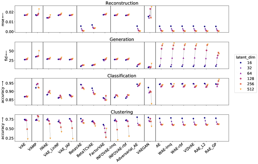
An important parameter of autoencoder models which is too often neglected in the literature is the dimension of the latent space. We now propose to keep the same configurations as previously but re-evaluate Tasks 1 to 5 with the latent space varying in the range $[16,32,64,128,256,512]$. Results are shown in Fig. 2 for MNIST and a ConvNet (see Appendix. D for CIFAR, ResNet and interpolations). For the generation task, we select the sampler with lowest FID on the validation set.

Assessing the influence of the latent dimension

A clear difference in behaviour is exhibited between variational-based and AE-based methods. For each given task, AEs share a common trend with respect to the evolution of the latent dimension: a common optimal latent dimension within the range $[16,32,64,128,256,512]$ is found for each task, but differs drastically among different tasks (e.g. 512 for reconstruction, 16 for generation, either 16 or 512 for classification and 512 for clustering with the MNIST dataset). This suggests the existence of a common intra-group optimal latent space dimension for a given task. In addition, we observe that $\beta$-VAE type methods (with the right hyper-parameter choice) can exhibit similar behaviours to AE models. The same observation can be made for variational-based methods, where it is interesting to note that although lower performances are achieved, the apparent optimal latent dimension varies less with respect to the choice of the task. Therefore, a latent dimension of 16 to 32 appears to be the optimal choice for all 4 Tasks on the MNIST dataset, and 32 to 128 on the CIFAR10 dataset. It should be noted that unsupervised tasks such as clustering of the latent representation of the CIFAR10 dataset are hard and models are expected to perform poorly, leading to less interpretable results.

Figure 2: From top to bottom: Evolution of the reconstruction MSE, generation FID, classification accuracy and clustering accuracy with respect to the latent space dimension on the MNIST dataset.

Table 1: Mean Squared Error ($10^{-3}$) and FID (lower is better) computed with 10k samples on the test set. For each model, the best configuration is the one achieving the lowest MSE on the validation set.

Model	ConvNet						ResNet
	MNIST (16)		CIFAR10 (256)		CELEBA (64)		MNIST (16)		CIFAR10 (256)		CELEBA (64)
	MSE $\downarrow$	FID $\downarrow$	MSE $\downarrow$	FID $\downarrow$	MSE $\downarrow$	FID $\downarrow$	MSE $\downarrow$	FID $\downarrow$	MSE $\downarrow$	FID $\downarrow$	MSE $\downarrow$	FID $\downarrow$
VAE	16.85	30.71	16.24	218.66	9.83	49.22	17.24	36.06	16.33	176.63	10.59	58.75
VAMP	24.17	44.95	17.45	221.40	10.81	51.64	17.11	37.58	16.87	177.03	11.50	60.89
IWAE	14.14	34.28	16.19	237.14	9.47	50.00	15.79	38.74	16.02	183.37	10.14	60.18
VAE-lin-NF	16.75	31.14	16.57	221.39	9.90	49.84	17.23	36.74	16.59	177.08	10.68	58.73
VAE-IAF	16.71	30.64	16.33	223.65	9.87	50.05	17.05	35.98	16.39	177.05	10.63	58.41
$\beta$-VAE	5.61	10.55	3.60	50.55	7.28	46.96	5.87	15.81	2.40	55.67	7.78	51.59
$\beta$-TC VAE	6.78	14.11	5.06	53.49	7.65	50.82	7.12	18.44	4.05	66.89	8.08	52.70
Factor VAE	17.27	30.39	16.41	224.3	10.16	53.61	18.13	37.97	16.55	176.8	10.93	59.46
InfoVAE-IMQ	16.65	30.62	16.19	216.44	9.81	50.51	17.17	37.33	16.32	173.79	10.63	58.04
InfoVAE-RBF	16.59	30.63	16.23	217.52	9.85	50.14	17.01	37.04	16.32	175.37	10.64	58.68
AAE	5.59	10.87	2.60	40.66	7.25	50.22	5.98	17.01	2.33	55.93	7.76	50.97
MSSSIM-VAE	32.60	37.91	39.42	276.70	35.60	124.52	33.67	40.25	39.61	254.34	35.43	119.92
VAEGAN	15.49	5.54	31.40	289.35	8.91	86.58	23.25	11.35	30.22	300.07	9.32	86.32
AE	5.47	11.61	2.82	41.98	7.03	51.08	6.13	13.74	2.34	55.43	7.74	50.54
WAE-IMQ	5.55	11.29	2.81	41.79	7.04	52.11	5.78	16.21	2.34	56.55	7.74	50.50
WAE-RBF	5.53	11.34	2.82	42.21	7.03	51.43	5.80	16.14	2.34	56.00	7.74	51.38
VQVAE	5.59	11.02	2.84	44.60	7.06	52.27	6.00	15.27	2.34	55.84	7.73	50.29
RAE-L2	5.24	15.37	2.25	49.28	6.90	53.98	5.76	17.27	2.35	57.85	7.74	51.07
RAE-GP	5.31	12.08	2.81	41.15	7.06	51.85	5.83	15.69	2.34	56.71	7.76	51.36

Table 2: Left: Mean test accuracy of a single layer classifier on the embedding obtained in the latent spaces of each model average on 20 runs. Right: Mean accuracy of 100 $k$-means fitted on the training embeddings coming from the autoencoders.

Model	Classification				Clustering
	ConvNet		ResNet		ConvNet		ResNet
	MNIST	CIFAR10	MNIST	CIFAR10	MNIST	CIFAR10	MNIST	CIFAR10
VAE	86.75 (0.05)	32.61 (0.03)	86.80 (0.03)	32.37 (0.03)	69.71 (2.01)	17.18 (0.68)	74.21 (0.97)	18.12 (0.74)
VAMP	92.17 (0.02)	33.46 (0.17)	92.58 (0.04)	33.03 (0.22)	67.26 (1.25)	24.03 (0.24)	72.48 (0.96)	23.35 (0.11)
IWAE	87.96 (0.04)	31.86 (0.04)	88.18 (0.03)	32.26 (0.04)	63.93 (1.73)	19.55 (0.67)	73.66 (2.30)	18.44 (0.86)
VAE-lin-NF	86.04 (0.04)	31.57 (0.02)	85.85 (0.05)	31.74 (0.03)	65.48 (2.76)	17.09 (0.64)	68.80 (3.65)	18.74 (0.68)
VAE-IAF	88.32 (0.02)	33.52 (0.02)	87.91 (0.02)	32.41 (0.02)	75.31 (1.69)	17.81 (0.73)	76.11 (2.15)	18.42 (0.66)
$\beta$-TC VAE	90.96 (0.02)	45.40 (0.05)	91.91 (0.02)	42.17 (0.07)	65.68 (0.91)	24.14 (0.65)	68.98 (2.67)	25.57 (0.61)
Factor VAE	86.08 (0.06)	31.38 (0.04)	83.44 (0.05)	31.76 (0.04)	51.02 (1.73)	15.77 (0.60)	60.79 (2.06)	17.56 (0.68)
InfoVAE-IMQ	86.33 (0.04)	32.48 (0.02)	86.31 (0.06)	32.10 (0.05)	68.17 (2.34)	16.65 (0.80)	71.31 (2.62)	18.10 (0.79)
InfoVAE-RBF	85.94 (0.03)	32.50 (0.03)	86.12 (0.04)	31.67 (0.03)	66.02 (1.14)	16.22 (0.69)	71.93 (1.91)	18.61 (0.67)
AAE	93.28 (0.03)	43.93 (0.07)	94.31 (0.03)	40.62 (0.11)	74.19 (3.22)	24.72 (0.75)	80.41 (2.09)	24.76 (0.53)
MSSSIM-VAE	78.30 (0.03)	20.26 (0.06)	76.54 (0.03)	20.24 (0.04)	49.33 (1.32)	11.70 (0.19)	48.58 (1.37)	11.70 (0.17)
VAEGAN	92.34 (0.02)	26.56 (0.04)	90.31 (0.03)	29.90 (0.03)	77.29 (1.19)	17.20 (0.45)	79.67 (0.90)	22.23 (0.44)
AE	93.81 (0.02)	42.15 (0.07)	94.26 (0.03)	40.47 (0.13)	73.55 (0.60)	23.19 (0.52)	77.30 (0.84)	23.18 (0.37)
WAE-IMQ	93.60 (0.02)	45.89 (0.07)	94.62 (0.03)	41.35 (0.03)	72.33 (2.92)	23.81 (0.61)	78.46 (3.48)	25.09 (0.82)
WAE-RBF	93.72 (0.02)	43.38 (0.08)	94.51 (0.02)	40.63 (0.08)	74.20 (1.94)	23.70 (0.71)	77.33 (1.92)	24.66 (0.63)
VQVAE	93.45 (0.02)	42.89 (0.07)	94.63 (0.04)	40.40 (0.09)	72.61 (0.40)	23.85 (0.48)	76.68 (2.36)	23.68 (0.37)
RAE-L2	94.75 (0.01)	42.76 (0.08)	94.43 (0.03)	40.22 (0.05)	74.07 (0.36)	23.77 (0.54)	78.66 (0.29)	24.84 (0.73)
RAE-GP	94.10 (0.02)	43.66 (0.07)	94.45 (0.02)	40.93 (0.14)	72.88 (0.52)	24.84 (0.53)	77.66 (1.29)	23.86 (0.32)

Table 3: Inception Score (higher is better) and FID (lower is better) computed with 10k samples on the test set. For each model and sampler we report the results obtained by the model achieving the lowest FID score on the validation set.

Model	Sampler	ConvNet						ResNet
		MNIST		CIFAR10		CELEBA		MNIST		CIFAR10		CELEBA
		FID $\downarrow$	IS $\uparrow$	FID	IS	FID	IS $\uparrow$	FID $\downarrow$	IS $\uparrow$	FID	IS	FID	IS
VAE	$\mathcal{N}$	28.5	2.1	241.0	2.2	54.8	1.9	31.3	2.0	181.7	2.5	66.6	1.6
	GMM	26.9	2.1	235.9	2.3	52.4	1.9	32.3	2.1	179.7	2.5	63.0	1.7
VAMP	VAMP	64.2	2.0	329.0	1.5	56.0	1.9	34.5	2.1	181.9	2.5	67.2	1.6
IWAE	$\mathcal{N}$	29.0	2.1	245.3	2.1	55.7	1.9	32.4	2.0	191.2	2.4	67.6	1.6
	GMM	28.4	2.1	241.2	2.1	52.7	1.9	34.4	2.1	188.8	2.4	64.1	1.7
VAE-lin NF	$\mathcal{N}$	29.3	2.1	240.3	2.1	56.5	1.9	32.5	2.0	185.5	2.4	67.1	1.6
	GMM	28.4	2.1	237.0	2.2	53.3	1.9	33.1	2.1	183.1	2.5	62.8	1.7
VAE-IAF	$\mathcal{N}$	27.5	2.1	236.0	2.2	55.4	1.9	30.6	2.0	183.6	2.5	66.2	1.6
	GMM	27.0	2.1	235.4	2.2	53.6	1.9	32.2	2.1	180.8	2.5	62.7	1.7
$\beta$-VAE	$\mathcal{N}$	21.4	2.1	115.4	3.6	56.1	1.9	19.1	2.0	124.9	3.4	65.9	1.6
	GMM	9.2	2.2	92.2	3.9	51.7	1.9	11.4	2.1	112.6	3.6	59.3	1.7
$\beta$-TC VAE	$\mathcal{N}$	21.3	2.1	116.6	2.8	55.7	1.8	20.7	2.0	125.8	3.4	65.9	1.6
	GMM	11.6	2.2	89.3	4.1	51.8	1.9	13.3	2.1	106.5	3.7	59.3	1.7
FactorVAE	$\mathcal{N}$	27.0	2.1	236.5	2.2	53.8	1.9	31.0	2.0	185.4	2.5	66.4	1.7
	GMM	26.9	2.1	234.0	2.2	52.4	2.0	32.7	2.1	184.4	2.5	63.3	1.7
InfoVAE - RBF	$\mathcal{N}$	27.5	2.1	235.2	2.1	55.5	1.9	31.1	2.0	182.8	2.5	66.5	1.6
	GMM	26.7	2.1	230.4	2.2	52.7	1.9	32.3	2.1	179.5	2.5	62.8	1.7
InfoVAE - IMQ	$\mathcal{N}$	28.3	2.1	233.8	2.2	56.7	1.9	31.0	2.0	182.4	2.5	66.4	1.6
	GMM	27.7	2.1	231.9	2.2	53.7	1.9	32.8	2.1	180.7	2.6	62.3	1.7
AAE	$\mathcal{N}$	16.8	2.2	139.9	2.6	59.9	1.8	19.1	2.1	164.9	2.4	64.8	1.7
	GMM	9.3	2.2	92.1	3.8	53.9	2.0	11.1	2.1	118.5	3.5	58.7	1.8
MSSSIM-VAE	$\mathcal{N}$	26.7	2.2	279.9	1.7	124.3	1.3	28.0	2.1	254.2	1.7	119.0	1.3
	GMM	27.2	2.2	279.7	1.7	124.3	1.3	28.8	2.1	253.1	1.7	119.2	1.3
VAEGAN	$\mathcal{N}$	8.7	2.2	199.5	2.2	39.7	1.9	12.8	2.2	198.7	2.2	122.8	2.0
	GMM	6.3	2.2	197.5	2.1	35.6	1.8	6.5	2.2	188.2	2.6	84.3	1.7
AE	$\mathcal{N}$	26.7	2.1	201.3	2.1	327.7	1.0	221.8	1.3	210.1	2.1	275.0	2.9
	GMM	9.3	2.2	97.3	3.6	55.4	2.0	11.0	2.1	120.7	3.4	57.4	1.8
WAE - RBF	$\mathcal{N}$	21.2	2.2	175.1	2.0	332.6	1.0	21.2	2.1	170.2	2.3	69.4	1.6
	GMM	9.2	2.2	97.1	3.6	55.0	2.0	11.2	2.1	120.3	3.4	58.3	1.7
WAE - IMQ	$\mathcal{N}$	18.9	2.2	164.4	2.2	64.6	1.7	20.3	2.1	150.7	2.5	67.1	1.6
	GMM	8.6	2.2	96.5	3.6	51.7	2.0	11.2	2.1	119.0	3.5	57.7	1.8
VQVAE	$\mathcal{N}$	28.2	2.0	152.2	2.0	306.9	1.0	170.7	1.6	195.7	1.9	140.3	2.2
	GMM	9.1	2.2	95.2	3.7	51.6	2.0	10.7	2.1	120.1	3.4	57.9	1.8
RAE-L2	$\mathcal{N}$	25.0	2.0	156.1	2.6	86.1	2.8	63.3	2.2	170.9	2.2	168.7	3.1
	GMM	9.1	2.2	85.3	3.9	55.2	1.9	11.5	2.1	122.5	3.4	58.3	1.8
RAE - GP	$\mathcal{N}$	27.1	2.1	196.8	2.1	86.1	2.4	61.5	2.2	229.1	2.0	201.9	3.1
	GMM	9.7	2.2	96.3	3.7	52.5	1.9	11.4	2.1	123.3	3.4	59.0	1.8

5 Conclusion

In this paper, we introduce Pythae, a new open-source Python library unifying common and state-of-the-art Generative AutoEncoder (GAE) implementations, allowing reliable and reproducible model training, data generation and experiment tracking. This library was designed as an open model testing environment driven by the community, wherein peers are encouraged to contribute by adding their own models, and by doing so favour reproducible research and accessibility to ready-to-use GAE models. As an illustration of the capabilities of Pythae, we perform a benchmarking of 19 generative autoencoder models on 5 downstream tasks (image reconstruction, generation, classification, clustering and interpolation) leading to some interesting findings on the general behaviours of generative autoencoder models. We hope that the library will continue to be adopted by the community and expand thanks to the increasing number of contributions.

Appendix A Usage of Pythae

In this section we illustrate through simple examples how to use Pythae pipelines. The library is documented and also available on pypi allowing a wider use and easier integration in other codes. All of the implementations proposed in the library are adaptations of the official code when available and allowed by the licence. If not, the method is re-implemented. Table. 4 lists all the implemented models as of June 2022.

1. Training configuration Before launching a model training, one must specify the training configuration that should be used. This can be done easily by instantiating a BaseTrainerConfig instance taking as input all the hyper-parameters related to the training (number of training epochs, learning rate to apply…). See the full documentation for additional arguments that can be passed to the BaseTrainerConfig.

            from pythae.trainers import BaseTrainerConfig        # Set up the model configuration        my_training_config = BaseTrainerConfig(            output_dir=’my_model’,            num_epochs=50,            learning_rate=1e-3,            batch_size=200) 

2. Model configuration Similarly to the TrainerConfig, the model can then be instantiated with the model configuration specifying any hyper-parameters relevant to the model. Note that each model has its own configuration with specific hyper-parameters. See the online documentation for more details.

            from pythae.models import BetaVAE, BetaVAEConfig        # Set up the model configuration        my_vae_config = BetaVAEConfig(            input_dim=(1, 28, 28),            latent_dim=16,            beta=2)        # Build the model        my_vae_model = BetaVAE(model_config=my_vae_config) 

3. Training A model training can then be launched by simply using the built-in training pipeline in which only the training/evaluation data need to be specified.

            from pythae.pipelines import TrainingPipeline        pipeline = TrainingPipeline(            training_config=my_training_config,            model=my_vae_model)        # Launch the Pipeline        pipeline(            train_data=your_train_data, # arrays or tensors            eval_data=your_eval_data) # arrays or tensors 

4. Model reloading The weights and configuration of the trained model can be reloaded using the AutoModel instance proposed in Pythae.

            from pythae.models import AutoModel        my_trained_vae = AutoModel.load_from_folder(’path/to/trained_model’) 

5. Data generation A data generation pipeline can be instantiated similarly to a model training. The pipeline can then be called with any relevant arguments such as the number of samples to generate or the training and evaluation data that may be needed to fit the sampler.

            from pythae.samplers import GaussianMixtureSamplerConfig        from pythae.pipelines import GenerationPipeline        # Define your sampler configuration        gmm_sampler_config = GaussianMixtureSamplerConfig(            n_components=10)        # Build the pipeline        pipeline = GenerationPipeline(            model=my_trained_vae,            sampler_config=gmm_sampler_config)        # Launch generation        generated_samples = pipeline(            num_samples=100,            return_gen=True,            train_data=train_data,            eval_data=None) 

Table 4: List of implemented VAEs

Name	Reference
Variational Autoencoder (VAE)	Kingma and Welling [37]
Beta Variational Autoencoder (BetaVAE)	Higgins et al. [30]
VAE with Linear Normalizing Flows (VAE_LinNF)	Rezende and Mohamed [55]
VAE with Inverse Autoregressive Flows (VAE_IAF)	Kingma et al. [38]
Disentangled $\beta$-VAE (DisentangledBetaVAE)	Higgins et al. [30]
Disentangling by Factorising (FactorVAE)	Kim and Mnih [35]
Beta-TC-VAE (BetaTCVAE)	Chen et al. [16]
Importance Weighted Autoencoder (IWAE)	Burda et al. [11]
VAE with perceptual metric similarity (MSSSIM_VAE)	Snell et al. [61]
Wasserstein Autoencoder (WAE)	Tolstikhin et al. [64]
Info Variational Autoencoder (INFOVAE_MMD)	Zhao et al. [72]
VAMP Autoencoder (VAMP)	Tomczak and Welling [65]
Hyperspherical VAE (SVAE)	Davidson et al. [23]
Adversarial Autoencoder (Adversarial_AE)	Makhzani [44]
Variational Autoencoder GAN (VAEGAN)	Larsen et al. [41]
Vector Quantized VAE (VQVAE)	Van Den Oord et al. [66]
Hamiltonian VAE (HVAE)	Caterini et al. [13]
Regularized AE with L2 decoder param (RAE_L2)	Ghosh et al. [27]
Regularized AE with gradient penalty (RAE_GP)	Ghosh et al. [27]
Riemannian Hamiltonian VAE (RHVAE)	Chadebec et al. [14]

Maintenance plan:

We intend for this library to be maintained in the long term. In that view, the main author’s contact details will remain available and up-to-date on the github repository, which will remain the main discussion channel. Additionally, we are currently considering adding back-up contributors that will also support this effort in the long-term. Since this library has already started to be a community effort with external contributors, we further hope that the community will also continue to help reviewing and updating the current implementations.

Original papers reproducibility

We validate the implementations by reproducing some results presented in the original publications when the official code has been released or when enough details about the experimental section of the papers were available (we indeed noted that in many papers key elements for reproducibility were missing such as the data split considered, which criteria is used to select the model on which the metrics are computed, the hyper-parameters are not fully disclosed or the network architectures is unclear making reproduction very hard if not impossible in certain cases). This insists on the fact that the framework is flexible enough to reproduce results from publications. Finally, we have open-sourced the scripts, configurations and results on the repository at https://github.com/clementchadebec/benchmark_VAE/tree/main/examples/scripts/reproducibility and made the trained models available on the HuggingFace Hub (e.g. https://huggingface.co/clementchadebec/reproduced_iwae).

Appendix B Interpolations

In this section, we show the interpolations obtained on the three considered datasets. For each model, we select both a starting image and an ending image from the test set and perform a linear interpolation between the corresponding embeddings in the learned latent space. We then show the decoded trajectory all along the interpolation line. For this task, we use the model configuration that obtained the lowest FID on the validation set with a GMM sampler from the generation task. We show the resulting interpolations for latent spaces of dimension 16 and 256 for MNIST, 32 and 256 for CIFAR10 and 64 for CELEBA. As mentioned in the paper, for this complex task, variational approaches tend to outperform the AE-based methods. This is well illustrated on MNIST with a latent space of dimension 256 since all the AE-based approaches eventually superpose the starting and ending image, making the interpolation visually irrelevant. Impressively, the regularisation imposed by the variational approaches prevents such undesirable behaviours from occurring. This adds to the observation made in Sec. 4.2.2 of the paper where we note some robustness to the latent dimension for the variational methods. Nonetheless, as stated in the paper this regularisation can also degrade image reconstruction, leading to very blurry interpolations, as illustrated on Fig. 5.

VAE
VAMP
IWAE
VAE-lin-NF
VAE-IAF
$\beta$-VAE
$\beta$-TC-VAE
Factor-VAE
InfoVAE - IMQ
InfoVAE - RBF

(a) MNIST (16)

(b) MNIST (256)

(c)

(d)

(e)

(f)

(g)

(h)

(i)

(j)

(k)

(l)

(m)

(n)

(o)

(p)

(q)

(r)

(s)

(t)

Figure 3: Interpolations on MNIST with the same starting and ending images for latent spaces of dimension 16 and 256. For each model we select the configuration achieving the lowest FID on the generation task on the validation set with a GMM sampler.

AAE
MSSSIM-VAE
VAEGAN
AE
WAE-IMQ
WAE-RBF
VQVAE
RAE-l2
RAE-GP

(a) MNIST (16)

(b) MNIST (256)

(c)

(d)

(e)

(f)

(g)

(h)

(i)

(j)

(k)

(l)

(m)

(n)

(o)

(p)

(q)

(r)

Figure 4: Interpolations on MNIST with the same starting and ending images for latent spaces of dimension 16 and 256. For each model we select the configuration achieving the lowest FID on the generation task on the validation set with a GMM sampler.

VAE
VAMP
IWAE
VAE-lin-NF
VAE-IAF
$\beta$-VAE
$\beta$-TC-VAE
Factor-VAE
InfoVAE - IMQ
InfoVAE - RBF

(a) CIFAR10 (32)

(b) CIFAR10 (256)

(c)

(d)

(e)

(f)

(g)

(h)

(i)

(j)

(k)

(l)

(m)

(n)

(o)

(p)

(q)

(r)

(s)

(t)

Figure 5: Interpolations on CIFAR10 with the same starting and ending images for latent spaces of dimension 32 and 256. For each model we select the configuration achieving the lowest FID on the generation task on the validation set with a GMM sampler.

AAE
MSSSIM-VAE
VAEGAN
AE
WAE-IMQ
WAE-RBF
VQVAE
RAE-l2
RAE-GP

(a) CIFAR10 (32)

(b) CIFAR10 (256)

(c)

(d)

(e)

(f)

(g)

(h)

(i)

(j)

(k)

(l)

(m)

(n)

(o)

(p)

(q)

(r)

Figure 6: Interpolations on CIFAR10 with the same starting and ending images for latent spaces of dimension 32 and 256. For each model we select the configuration achieving the lowest FID on the generation task on the validation set with a GMM sampler.

VAE
VAMP
IWAE
VAE-lin-NF
VAE-IAF
$\beta$-VAE
$\beta$-TC-VAE
Factor-VAE
InfoVAE - IMQ
InfoVAE - RBF

(a) CELEBA (64)

(b) CELEBA (64)

(c)

(d)

(e)

(f)

(g)

(h)

(i)

(j)

(k)

(l)

(m)

(n)

(o)

(p)

(q)

(r)

(s)

(t)

Figure 7: Interpolations on CELEBA with the same starting and ending images for a latent space of dimension 64. For each model we select the configuration achieving the lowest FID on the generation task on the validation set with a GMM sampler.

AAE
MSSSIM-VAE
VAEGAN
AE
WAE-IMQ
WAE-RBF
VQVAE
RAE-l2
RAE-GP

(a) CELEBA (64)

(b) CELEBA (64)

(c)

(d)

(e)

(f)

(g)

(h)

(i)

(j)

(k)

(l)

(m)

(n)

(o)

(p)

(q)

(r)

Figure 8: Interpolations on CELEBA with the same starting and ending images for a latent space of dimension 64. For each model we select the configuration achieving the lowest FID on the generation task on the validation set with a GMM sampler.

Appendix C Detailed experiments set-up

We detail here the main experimental set-up and implementation choices made in the benchmark. We let the reader refer to the code available online for specific implementation aspects

The data

To perform the benchmaks presented in the paper, we select 3 classical free-to-use image datasets: MNIST [42], CIFAR10 [40] and CELEBA [43]. These datasets are publicly available, widely used for generative model related papers and have well known associated metrics in the literature. Each dataset is split into a train set, a validation set and a test set. For MNIST and CIFAR10 the validation set is composed of the last 10k images extracted from the official train set and the test set corresponds to the official one. For CELEBA, we use the official train/val/test split.

Training paradigm

We equip each model used in the benchmark with the same neural network architecture for both the encoder and decoder, taken as a ConvNet and ResNet (architectures given in Tables. 5 and 6) leading to a comparable number of parameters . For the 19 considered models, due to computational limitations, 10 different configurations are considered, allowing a simple exploration of the models’ hyper-parameters. The sets of hyper-parameters explored are detailed in Appendix. D for each model. The models are then trained on MNIST and CIFAR10 for 100 epochs, a starting learning rate of $1e^{-4}$ and batch size of 100 with Adam optimizer [36]. A scheduler reducing the learning rate by half if the validation loss does not improve for 10 epochs is also used. For CELEBA, we use the same setting but we train the models for 50 epochs with a starting learning rate of $1e^{-3}$. Models with unstable training (NaN, huge training spikes…) are iteratively retrained with a starting learning rate divided by 10 until training stabilises. All 19 models are trained on a single 32GB V100 GPU. This leads to 10 trained models for each method, each dataset (MNIST, CIFAR10 or CELEBA) and each neural network (ConvNet or ResNet) leading to a total of 1140 models. The training setting (curves, configs …) can be found at https://wandb.ai/benchmark_team/trainings.

Sampling paradigm for the MAF and VAE samplers

For the Masked Autoregressive Flow sampler used for sampling we use a 3-layer MADE [26] with 128 hidden units and ReLU activation for each layer and stack 2 blocks of MAF to create the flow. For the masked layers, the mask is made sequentially and the ordering is reversed between each MADE. For this normalising flow we consider a starting distribution given by a standard Gaussian. For the auxiliary VAE sampling method proposed in [22], we consider a simple VAE with a Multi Layer Perceptron (MLP) encoder and decoder, with 2 hidden layers composed of 1024 units and ReLU activation. Both samplers are fitted with 200 epochs using the train and evaluation embeddings coming from the trained autoencoder models. A learning rate of $1e^{-4}$, a scheduler decreasing the learning rate by half if the validation loss does not improve for 10 epochs and a batch size of 100 are used for these samplers.

Table 5: Neural network architecture used for the convolutional networks.

	MNIST	CIFAR10	CELEBA
Encoder	(1, 28, 28)	(3, 32, 32)	(3, 64, 64)
Layer 1	Conv(128, 4, 2), BN, ReLU	Conv(128, 4, 2), BN, ReLU	Conv(128, 4, 2), BN, ReLU
Layer 2	Conv(256, 4, 2), BN, ReLU	Conv(256, 4, 2), BN, ReLU	Conv(256, 4, 2), BN, ReLU
Layer 3	Conv(512, 4, 2), BN, ReLU	Conv(512, 4, 2), BN, ReLU	Conv(512, 4, 2), BN, ReLU
Layer 4	Conv(1024, 4, 2), BN, ReLU	Conv(1024, 4, 2), BN, ReLU	Conv(1024, 4, 2), BN, ReLU
Layer 5	Linear(1024, latent_dim)*	Linear(4096, latent_dim)*	Linear(16384, latent_dim)*
Decoder
Layer 1	Linear(latent_dim, 16384)	Linear(latent_dim, 65536)	Linear(latent_dim, 65536)
Layer 2	ConvT(512, 3, 2), BN, ReLU	ConvT(512, 4, 2), BN, ReLU	ConvT(512, 5, 2), BN, ReLU
Layer 3	ConvT(256, 3, 2), BN, ReLU	ConvT(256, 4, 2), BN, ReLU	ConvT(256, 5, 2), BN, ReLU
Layer 4	Conv(1, 3, 2), Sigmoid	Conv(3, 4, 1), Sigmoid	ConvT(128, 5, 2), BN, ReLU
Layer 5	-	-	ConvT(3, 5, 1), Sigmoid
*Doubled for VAE-based models

Table 6: Neural network architecture used for the residual networks.

	MNIST	CIFAR10	CELEBA
Encoder	(1, 28, 28)	(3, 32, 32)	(3, 64, 64)
Layer 1	Conv(64, 4, 2)	Conv(64, 4, 2)	Conv(64, 4, 2)
Layer 2	Conv(128, 4, 2)	Conv(128, 4, 2)	Conv(128, 4, 2)
Layer 3	Conv(128, 3, 2)	Conv(128, 3, 1)	Conv(128, 3, 2)
Layer 4	ResBlock**	ResBlock**	Conv(128, 3, 2)
Layer 5	ResBlock**	ResBlock**	ResBlock**
Layer 6	Linear(2048, latent_dim)*	Linear(8192, latent_dim)*	ResBlock**
Layer 7	-	-	Linear(2048, latent_dim)*
Decoder
Layer 1	Linear(latent_dim, 2048)	Linear(latent_dim, 8192)	Linear(latent_dim, 2048)
Layer 2	ConvT(128, 3, 2)	ResBlock**	ConvT(128, 3, 2)
Layer 3	ResBlock**	ResBlock**	ResBlock**
Layer 4	ResBlock**, ReLU	ConvT(64, 4, 2)	ResBlock**
Layer 5	ConvT(64, 3, 2), ReLU	ConvT(3, 4, 2), Sigmoid	ConvT(128, 5, 2), Sigmoid
Layer 6	ConvT(1, 3, 2), Sigmoid	-	ConvT(64, 5, 2), Sigmoid
Layer 6	-	-	ConvT(3, 4, 2), Sigmoid
*Doubled for VAE-based models
**The ResBlocks are composed of one Conv(32, 3, 1) followed by Conv(128, 1, 1) with ReLU.

Appendix D Additional results

D.1 Effect of the latent dimension on the 4 tasks with the CIFAR10 database

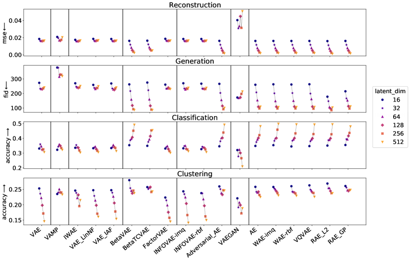
Analogously to the results shown in the paper on the MNIST dataset for the 4 chosen tasks (reconstruction, generation, classification and clustering), Fig. 9 shows the impact the choice of the latent space dimension has on the performances of the models on the CIFAR10 dataset, whose image arguably have a greater intrinsic latent dimension than images of the MNIST dataset. Similarly to MNIST, two distinct groups appear: the AE-based methods and variational methods. Again, for all tasks but clustering, variational based methods demonstrate good robustness properties with respect to the dimension of the latent space when compared to AE approaches.

Figure 9: From top to bottom: Evolution of the reconstruction MSE, generation FID, classification accuracy and clustering accuracy with respect to the latent space dimension on the CIFAR dataset.

D.2 Complete generation table

In Table. 7 are presented the full results obtained for generation i.e. including the MAF and 2-stage VAE sampler [22]. As mentioned in the paper, it is interesting to note that fitting a GMM instead of using the prior for the variational-based approaches seems to often allow a better image generation since it allows a better prospecting of the learned latent space of each model. Interestingly, it seems that fitting more complex density estimators such as a normalising flow (MAF sampler) or another VAE (2-stage sampler) does not improve the generation results when compared to the GMM for those datasets.

Table 7: Inception Score (higher is better) and FID (lower is better) computed with 10k samples on the test set. For each model and sampler we report the results obtained by the model achieving the lowest FID score on the validation set.

Model	Sampler	ConvNet						ResNet
		MNIST		CIFAR10		CELEBA		MNIST		CIFAR10		CELEBA
		FID $\downarrow$	IS $\uparrow$	FID	IS	FID	IS $\uparrow$	FID $\downarrow$	IS $\uparrow$	FID	IS	FID	IS
	$\mathcal{N}$	28.5	2.1	241.0	2.2	54.8	1.9	31.3	2.0	181.7	2.5	66.6	1.6
	GMM	26.9	2.1	235.9	2.3	52.4	1.9	32.3	2.1	179.7	2.5	63.0	1.7
	VAE	40.3	2.0	337.5	1.7	70.9	1.6	48.7	1.8	358.0	1.3	76.4	1.4
VAE	MAF	26.8	2.1	239.5	2.2	52.5	2.0	31.0	2.1	181.5	2.5	62.9	1.7
VAMP	VAMP	64.2	2.0	329.0	1.5	56.0	1.9	34.5	2.1	181.9	2.5	67.2	1.6
	$\mathcal{N}$	29.0	2.1	245.3	2.1	55.7	1.9	32.4	2.0	191.2	2.4	67.6	1.6
	GMM	28.4	2.1	241.2	2.1	52.7	1.9	34.4	2.1	188.8	2.4	64.1	1.7
	VAE	42.4	2.0	346.6	1.5	74.3	1.5	50.1	1.9	364.8	1.2	76.4	1.4
IWAE	MAF	28.1	2.1	243.4	2.1	52.7	1.9	32.5	2.1	190.4	2.4	64.3	1.7
VAE-lin NF	$\mathcal{N}$	29.3	2.1	240.3	2.1	56.5	1.9	32.5	2.0	185.5	2.4	67.1	1.6
	GMM	28.4	2.1	237.0	2.2	53.3	1.9	33.1	2.1	183.1	2.5	62.8	1.7
	VAE	40.1	2.0	311.0	1.6	71.1	1.6	49.7	1.9	296.2	1.7	75.6	1.4
	MAF	27.7	2.1	239.1	2.1	53.4	2.0	32.4	2.0	184.2	2.5	62.7	1.7
	$\mathcal{N}$	27.5	2.1	236.0	2.2	55.4	1.9	30.6	2.0	183.6	2.5	66.2	1.6
	GMM	27.0	2.1	235.4	2.2	53.6	1.9	32.2	2.1	180.8	2.5	62.7	1.7
	VAE	39.4	2.0	330.5	1.1	73.0	1.5	44.8	1.9	322.7	1.5	76.7	1.4
VAE-IAF	MAF	26.9	2.1	236.8	2.2	53.6	1.9	30.6	2.1	182.5	2.5	63.0	1.7
$\beta$-VAE	$\mathcal{N}$	21.4	2.1	115.4	3.6	56.1	1.9	19.1	2.0	124.9	3.4	65.9	1.6
	GMM	9.2	2.2	92.2	3.9	51.7	1.9	11.4	2.1	112.6	3.6	59.3	1.7
	VAE	14.0	2.2	139.6	3.6	55.0	1.9	20.3	2.1	152.5	3.5	61.5	1.7
	MAF	9.5	2.2	100.9	3.5	51.5	2.0	12.0	2.1	120.0	3.6	59.7	1.8
	$\mathcal{N}$	21.3	2.1	116.6	2.8	55.7	1.8	20.7	2.0	125.8	3.4	65.9	1.6
	GMM	11.6	2.2	89.3	4.1	51.8	1.9	13.3	2.1	106.5	3.7	59.3	1.7
	VAE	18.4	2.2	127.9	4.2	59.7	1.8	28.3	2.0	164.0	3.3	66.4	1.5
$\beta$-TC VAE	MAF	12.0	2.2	95.6	3.6	52.2	1.9	13.7	2.1	116.6	3.4	60.1	1.7
FactorVAE	$\mathcal{N}$	27.0	2.1	236.5	2.2	53.8	1.9	31.0	2.0	185.4	2.5	66.4	1.7
	GMM	26.9	2.1	234.0	2.2	52.4	2.0	32.7	2.1	184.4	2.5	63.3	1.7
	VAE	41.2	1.9	338.3	1.5	75.0	1.5	54.7	1.8	316.2	1.3	77.7	1.4
	MAF	26.7	2.2	236.7	2.2	52.7	1.9	32.8	2.1	185.8	2.5	63.4	1.7
	$\mathcal{N}$	27.5	2.1	235.2	2.1	55.5	1.9	31.1	2.0	182.8	2.5	66.5	1.6
	GMM	26.7	2.1	230.4	2.2	52.7	1.9	32.3	2.1	179.5	2.5	62.8	1.7
	VAE	39.7	2.0	327.2	1.5	73.7	1.5	50.6	1.9	363.4	1.2	75.8	1.4
InfoVAE - RBF	MAF	25.9	2.1	233.5	2.2	52.2	2.0	30.5	2.1	181.3	2.5	62.7	1.7
InfoVAE - IMQ	$\mathcal{N}$	28.3	2.1	233.8	2.2	56.7	1.9	31.0	2.0	182.4	2.5	66.4	1.6
	GMM	27.7	2.1	231.9	2.2	53.7	1.9	32.8	2.1	180.7	2.6	62.3	1.7
	VAE	40.4	1.9	323.8	1.6	73.7	1.5	49.9	1.9	341.8	1.8	75.7	1.4
	MAF	27.2	2.1	232.3	2.1	53.8	2.0	30.6	2.1	182.5	2.5	62.6	1.7
	$\mathcal{N}$	16.8	2.2	139.9	2.6	59.9	1.8	19.1	2.1	164.9	2.4	64.8	1.7
	GMM	9.3	2.2	92.1	3.8	53.9	2.0	11.1	2.1	118.5	3.5	58.7	1.8
	VAE	13.4	2.2	144.0	3.4	58.2	1.8	15.1	2.1	145.2	3.6	59.0	1.7
AAE	MAF	9.3	2.2	101.1	3.2	53.8	2.0	11.9	2.1	133.6	3.1	59.2	1.8
MSSSIM-VAE	$\mathcal{N}$	26.7	2.2	279.9	1.7	124.3	1.3	28.0	2.1	254.2	1.7	119.0	1.3
	GMM	27.2	2.2	279.7	1.7	124.3	1.3	28.8	2.1	253.1	1.7	119.2	1.3
	VAE	51.2	1.9	355.5	1.1	137.9	1.2	51.6	1.9	372.1	1.1	136.5	1.2
	MAF	26.9	2.2	279.8	1.7	124.0	1.3	27.5	2.1	254.1	1.7	119.5	1.3
	$\mathcal{N}$	8.7	2.2	199.5	2.2	39.7	1.9	12.8	2.2	198.7	2.2	122.8	2.0
	GMM	6.3	2.2	197.5	2.1	35.6	1.8	6.5	2.2	188.2	2.6	84.3	1.7
	VAE	11.2	2.1	310.9	2.0	54.5	1.6	9.2	2.1	272.7	2.0	88.8	1.6
VAEGAN	MAF	6.9	2.3	199.0	2.1	36.7	1.8	6.6	2.2	191.9	2.5	84.8	1.7
AE	$\mathcal{N}$	26.7	2.1	201.3	2.1	327.7	1.0	221.8	1.3	210.1	2.1	275.0	2.9
	GMM	9.3	2.2	97.3	3.6	55.4	2.0	11.0	2.1	120.7	3.4	57.4	1.8
	MAF	9.9	2.2	108.3	3.1	55.7	2.0	12.0	2.1	136.5	3.0	58.3	1.8
	$\mathcal{N}$	21.2	2.2	175.1	2.0	332.6	1.0	21.2	2.1	170.2	2.3	69.4	1.6
	GMM	9.2	2.2	97.1	3.6	55.0	2.0	11.2	2.1	120.3	3.4	58.3	1.7
WAE - RBF	MAF	9.8	2.2	108.2	3.1	56.0	2.0	11.8	2.2	135.3	3.0	58.3	1.8
WAE - IMQ	$\mathcal{N}$	18.9	2.2	164.4	2.2	64.6	1.7	20.3	2.1	150.7	2.5	67.1	1.6
	GMM	8.6	2.2	96.5	3.6	51.7	2.0	11.2	2.1	119.0	3.5	57.7	1.8
	MAF	9.5	2.2	107.8	3.1	51.6	2.0	11.8	2.1	130.2	3.0	58.7	1.7
	$\mathcal{N}(0,1)$	28.2	2.0	152.2	2.0	306.9	1.0	170.7	1.6	195.7	1.9	140.3	2.2
	GMM	9.1	2.2	95.2	3.7	51.6	2.0	10.7	2.1	120.1	3.4	57.9	1.8
VQVAE	MAF	9.6	2.2	104.7	3.2	52.3	1.9	11.7	2.2	136.8	3.0	57.9	1.8
RAE-L2	$\mathcal{N}$	25.0	2.0	156.1	2.6	86.1	2.8	63.3	2.2	170.9	2.2	168.7	3.1
	GMM	9.1	2.2	85.3	3.9	55.2	1.9	11.5	2.1	122.5	3.4	58.3	1.8
	MAF	9.5	2.2	93.4	3.5	55.2	2.0	12.3	2.2	136.6	3.0	59.1	1.7
	$\mathcal{N}$	27.1	2.1	196.8	2.1	86.1	2.4	61.5	2.2	229.1	2.0	201.9	3.1
	GMM	9.7	2.2	96.3	3.7	52.5	1.9	11.4	2.1	123.3	3.4	59.0	1.8
RAE - GP	MAF	9.7	2.2	106.3	3.2	52.5	1.9	12.2	2.2	139.4	3.0	59.5	1.8

D.3 Further interesting results

Generated samples

In addition to quantitative metrics, we also provide in Fig. 10 and Fig. 11 some samples coming from the different models using either a $\mathcal{N}(0,I_{d})$ or fitting a GMM with 10 components on MNIST and CELEBA. This allows to visually differentiate the quality of the different sampling methods.

VAE
IWAE
VAE-lin-NF
VAE-IAF
$\beta$-VAE
$\beta$-TC-VAE
Factor-VAE
InfoVAE - IMQ
InfoVAE - RBF
AAE
MSSSIM-VAE
VAEGAN
AE
WAE-IMQ
WAE-RBF
VQVAE
RAE-L2
RAE-GP

(a) MNIST - $\mathcal{N}$

(b) MNIST - GMM

(c)

(d)

(e)

(f)

(g)

(h)

(i)

(j)

(k)

(l)

(m)

(n)

(o)

(p)

(q)

(r)

(s)

(t)

(u)

(v)

(w)

(x)

(y)

(z)

(aa)

(ab)

(ac)

(ad)

(ae)

(af)

(ag)

(ah)

(ai)

(aj)

Figure 10: Generated samples on MNIST for a latent space of dimension 16 and ConvNet architecture. For each model, we select the configuration achieving the lowest FID on the validation set.

VAE
IWAE
VAE-lin-NF
VAE-IAF
$\beta$-VAE
$\beta$-TC-VAE
Factor-VAE
InfoVAE - IMQ
InfoVAE - RBF
AAE
MSSSIM-VAE
VAEGAN
AE
WAE-IMQ
WAE-RBF
VQVAE
RAE-L2
RAE-GP

(a) CELEBA - $\mathcal{N}$

(b) CELEBA - GMM

(c)

(d)

(e)

(f)

(g)

(h)

(i)

(j)

(k)

(l)

(m)

(n)

(o)

(p)

(q)

(r)

(s)

(t)

(u)

(v)

(w)

(x)

(y)

(z)

(aa)

(ab)

(ac)

(ad)

(ae)

(af)

(ag)

(ah)

(ai)

(aj)

Figure 11: Generated samples on CELEBA for a latent space of dimension 64 and ConvNet architecture. For each model, we select the configuration achieving the lowest FID on the validation set.

Sampler ablation study

Fig. 12 shows the same results as Table. 7 but under a different prism. In this plot, we show the influence each sampler has on the generation quality for all the models considered in this study. Note that sampling using a $\mathcal{N}(0,I_{d})$ for an AE, RAE or VQVAE is far from being optimal since those models do not enforce explicitly the latent variables to follow this distribution. As mentioned in the paper, this experiment shows that using more complex density estimators such as a GMM or a normalising flow almost always improves the generation metric.

Figure 12: Evolution of the FID for the generation task depending on the sampler, for a ConvNet, the MNIST dataset and a latent dimension of 16. For each sampler and model, we select the configuration achieving the lowest FID on the validation set.

Neural network architecture ablation study

As explained in the paper and in Appendix. C, we consider two different neural architectures for the encoder and decoder of each model: a ConvNet (convolutional neural network) and a ResNet (residual neural network). Fig. 13 shows the influence the choice of the neural architecture has on the ability of the model to perform the 4 tasks presented in the paper. The results are computed for each model on MNIST and a latent dimension of 16. The ConvNet architecture has approximately 20 times more parameters than the ResNet in such conditions. We select the best configuration for each model and each task on the validation set and report the results on the test set. Unsuprisingly, we see in Fig. 13 that the ConvNet architecture, more adapted to capture features intrinsic to images, leads to the best performances for reconstruction and generation. Interestingly, the ResNet outperforms the ConvNet for the classification and clustering tasks, meaning that in addition to the network complexity, its structure can play a major role in the representation learned by the models.

Figure 13: Evolution of the metrics for the 4 tasks depending on the network type on the MNIST dataset and a latent dimension of 16.

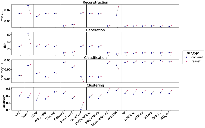
Training time

Fig. 14 shows the training times required for each model for both network architectures on the MNIST dataset. For each model, we show the results obtained with the configuration giving the best performances on the generation task with fixed latent dimension 16. It is interesting to note that although VAEGAN outperforms other models on the generation task, it is at the price of a higher computational time. This is due to the discriminator network (a convolutional neural net) that is called several times during training and takes images as inputs. It should be noted that methods applying normalising flows to the posterior (VAE-lin-NF and VAE-IAF) maintain a reasonable training time, as the flows were chosen for their scalability.

Figure 14: Total training time for the models trained on the MNIST dataset with latent dimension 16 with the best performance on the generation task.

D.4 Configurations and results by models

In this section we briefly explain each model considered in the benchmark, and show the evolution of performances on the 4 tasks and the training speed with respect to the choice of the hyper-parameters. For all 4 tasks we consider the MNIST dataset and a fixed latent space of dimension 16, as well as the Normal Gaussian sampler (if applicable) and the convolutional network architecture. For each model, 10 configuration runs with different hyper-parameters were tested. It should be noted that this configuration search was done empirically and is not exhaustive, therefore models with multiple hyper-parameters or that are sensitive to the choice of hyper-parameters will tend to have sub-optimal configuration choices. Although hyper-parameter choices are dependant on both the auto-encoder architecture and the dataset, it is interesting to note the relative evolution of the performances on the different tasks and the training time induced by different hyper-parameter choices.

Notations

In order to better underline the differences between different models and for clarity purposes, we set the following unified notations:

• $X=\{x_{1},\dots,x_{N}\}\in\mathcal{X}^{N}$ the input dataset

• $x\in\mathcal{X}$ an observation from the dataset, and $z\in\mathcal{Z}=\mathbb{R}^{d}$ its corresponding latent vector

• $\hat{x}$ the reconstruction of $x$ by the auto-encoder model

• $p_{z}(z)$ the prior distribution, with $p_{z}\equiv\mathcal{N}(0,I_{d})$ under standard VAE assumption

• $q_{\phi}(z|x)$ the approximate posterior distribution, modelled by the encoder. Kingma and Welling [37] set

  $$q_{\phi}(z|x)\equiv\mathcal{N}\big{(}\mu_{\phi}(x),\Sigma_{\phi}(x))\big{)}$$

  where $\Sigma_{\phi}(x)=diag[\sigma_{\phi}(x)]$ and $\big{(}\mu_{\phi}(x),\sigma_{\phi}(x)\big{)}\in\mathbb{R}^{2\times d}$ are outputs of the encoder network. The sampling process $z\sim q_{\phi}(z|x)$ is therefore performed by sampling $\varepsilon\sim\mathcal{N}(0,I_{d})$ and setting $z=\mu_{\phi}(x)+\Sigma_{\phi}(x)^{1/2}\cdot\varepsilon$ (re-parametrization trick).

• $p_{\theta}(x|z)$ the distribution of $x$ given $z$

• $p_{\theta}(x)=\int_{\mathcal{Z}}p_{\theta}(x|z)p_{z}(z)dz$ the marginal distribution of $x$

• $q_{\phi}(z)=\dfrac{1}{N}\sum_{i=1}^{N}q_{\phi}(z|x_{i})$ the aggregated posterior integrated over the training set.

• $\mathcal{D}_{KL}$ the Kullback-Leibler divergence

We further recall that Kingma and Welling [37] use the unbiased estimate $\widehat{p}_{\theta}(x)$ of ${p}_{\theta}(x)$ defined as

$$\widehat{p}_{\theta}(x)=\frac{p_{\theta}(x|z)p_{z}(z)}{q_{\phi}(z|x)}$$

to derive the standard Evidence Lower Bound (ELBO) of the log probability $\log p_{\theta}(x)$ which we wish to maximize:

$$\mathcal{L}_{ELBO}=\mathbb{E}_{x\sim p_{\theta}(x)}\big{[}\mathcal{L}_{ELBO}(x)\big{]}$$

with

$$\mathcal{L}_{ELBO}(x)=\underbrace{\mathbb{E}_{z\sim q_{\phi}}[\log p_{\theta}(x|z)]}_{\text{reconstruction}}-\underbrace{\mathcal{D}_{KL}\big{[}q_{\phi}(z|x)||p_{z}(z)\big{]}}_{\text{regularisation}}$$

The reconstruction loss is maximized when $\hat{x}$ is close to $x$, thus encouraging a good reconstruction of the input $x$, while the regularisation term is maximized when $q_{\phi}(z|x)$ is close to $p_{z}(z)$, encouraging the posterior distribution to follow the chosen prior distribution.

The integration over $p_{\theta}(x)$ is approximated by the empirical distribution of the training dataset, and the negative ELBO function acts as a loss function to minimize for the encoder and decoder networks.

VAE with a VampPrior (VAMP)

Starting from the observation that a standard Gaussian prior may be too simplistic, Tomczak and Welling [65] proposes a less restrictive prior: the Variational Mixture of Posteriors (VAMP). A VAE with a VAMP prior aims at relaxing the posterior constraint by replacing the conventional normal prior with a multimodal aggregated posterior given by:

$$p_{z}(z)=\frac{1}{K}\sum_{k=1}^{K}q_{\phi}(z|u_{k})\,,$$

where $u_{k}$ are pseudo-inputs living in the data space $\mathcal{X}$ learned through back-propagation and acting as anchor points for the prior distribution. For the VAMP VAE implementation, we use the same architecture as the authors’ implementation for the network generating the pseudo-inputs: a MLP with a single layer and Tanh activation.

Results by configuration

Table 8: VAMP configurations

Config	1	2	3	4	5	6	7	8	9	10
Number of pseudo-inputs (K)	10	20	30	500	100	150	200	250	300	500

Figure 15: Results on VAMP

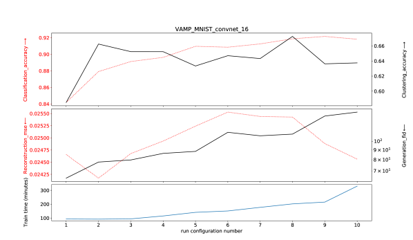
Importance Weighted Autoencoder (IWAE)

Burda et al. [11] introduce an alternative lower bound to maximize, derived from importance weighting where the new unbiased estimate $\widehat{p}_{\theta}(x)$ of the marginal distribution $p_{\theta}(x)$ is computed with $L$ samples $z_{1},\dots,z_{L}\sim q_{\phi}(z|x)$ :

$$\widehat{p}_{\theta}(x)=\dfrac{1}{L}\sum_{i=1}^{L}\frac{p_{\theta}(x|z_{i})p_{z}(z_{i})}{q_{\phi}(z_{i}|x)}\,.$$

This estimate induces a new lower bound of the true marginal distribution $p_{\theta}(x)$ using Jensen’s inequality:

$$\mathcal{L}_{\text{IWAE}}(x):=\mathbb{E}_{z_{1},\dots,z_{L}\sim q(z|x)}\bigg{[}\log\frac{1}{L}\sum\limits_{i=1}^{L}\frac{p_{\theta}(x|z_{i})p_{z}(z_{i})}{q_{\phi}(z_{i}|x)}\bigg{]}\leq\log\underbrace{\mathbb{E}_{z_{1},\dots,z_{L}\sim q(z|x)}\big{[}\widehat{p}_{\theta}(x)\big{]}}_{p_{\theta}(x)}.$$

As the number of samples $L$ increases, $\mathcal{L}_{\text{IWAE}}(x)$ becomes closer to $\log p_{\theta}(x)$, therefore providing a tighter bound on the true objective. Note that when $L=1$ we recover the original VAE framework.

As expected the reconstruction quality increases with the number of samples. Nonetheless, we note that increasing the number of samples has a significant impact on the computation of a single training step, therefore leading to a much slower training process.

Results by configuration

Table 9: IWAE configurations

Config	1	2	3	4	5	6	7	8	9	10
Number of samples (L)	2	3	4	5	6	7	8	9	10	12

Figure 16: Results on IWAE

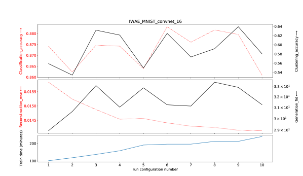
Variational Inference with Normalizing Flows (VAE-lin-NF)

In order to model a more complex family of approximate posterior distributions, Rezende and Mohamed [55] propose to use a succession of normalising flows to transform the simple distribution $q_{\phi}(z|x)$, allowing it to model more complex behaviours. In practice, after having sampled $z_{0}\sim q_{\phi}(z|x)$, $z_{0}$ is passed through a chain of $K$ invertible smooth mappings from the latent space $\mathbb{R}^{d}$ to itself:

$$z_{K}=f_{K}\circ\dots\circ f_{2}\circ f_{1}(z_{0})\,.$$

The modified latent vector $z_{K}$ is then used as input $z$ for the decoder network. In their paper, the authors propose to use two types of transformations: planar and radial flows.

$$f_{\mathrm{planar}}(z)=z+uh(w^{\top}z+b)\hskip 14.22636pt;\hskip 14.22636ptf_{\mathrm{radial}}(z)=z+\beta g(\alpha,r)(z-z_{0})\,,$$

where $h$ is a smooth non-linearity with tractable derivatives and $g(\alpha,r)=\frac{1}{\alpha+r}$. The parameters are such that $r=\|z-z_{0}\|$, $u,w,z_{0}\in\mathbb{R}^{d}$, $\alpha\in\mathbb{R}^{+}$ and $b,\beta\in\mathbb{R}$. We can easily compute the resulting density $q$ given by

$$\log q(z_{K})=\log q_{\phi}(z_{0}|x)-\sum\limits_{k=1}^{K}\log\bigg{|}\det\frac{\partial f_{k}}{\partial z}\bigg{|}\,.$$

This makes the ELBO tractable and optimisation possible.

Results by configuration

Table 10: VAE-lin-NF configurations

Config	1	2	3	4	5	6	7	8	9	10
Flow sequence	PPPPP	RRRRR	PRPRP	10P	15P	20P	30P	PRPRPRPRPR	PPP	PRPPRPPPPR
‘P’ stands for planar flow - ‘R’ stands for radial flow

Figure 17: Results on VAE-lin-NF

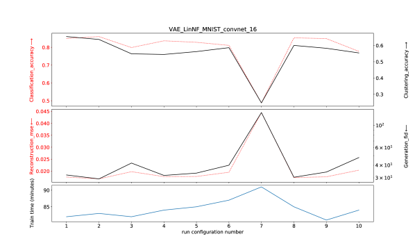
Variational Inference with Inverse Autoregressive Flow (VAE-IAF)

Kingma et al. [38] improve upon the works of [55] with a new type of normalising flow that better scales to high-dimensional latent spaces. The main idea is again to apply several transformations to a sample from a simple distribution in order to model richer distributions. Starting from $z_{0}\sim q_{\phi}(z|x)$, the proposed IAF flow consists in applying consecutively the following transformation

$$z_{k}=\mu_{k}+\sigma_{k}\cdot z_{k-1}\,,$$

where $\mu_{k}$ and $\sigma_{k}$ are the outputs of an autoregressive neural network taking $z_{k-1}$ as input. Inspired from the original paper, to implement one Inverse Autoregressive Flow we use MADE [26] and stack multiple IAF together to create a richer flow. The MADE mask is made sequentially for the masked autoencoders and the ordering is reversed after each MADE.

Results by configuration

Table 11: VAE-IAF configurations

Config	1	2	3	4	5	6	7	8	9	10
hidden size in MADE	32.0	32.0	32.0	32.0	32.0	32.0	32.0	32.0	64.0	128.0
number hidden units in MADE	2.0	2.0	2.0	2.0	2.0	2.0	4.0	6.0	2.0	2.0
number of IAF blocks	1.0	2.0	5.0	10.0	20.0	4.0	4.0	4.0	4.0	4.0

Figure 18: Results on VAE-IAF

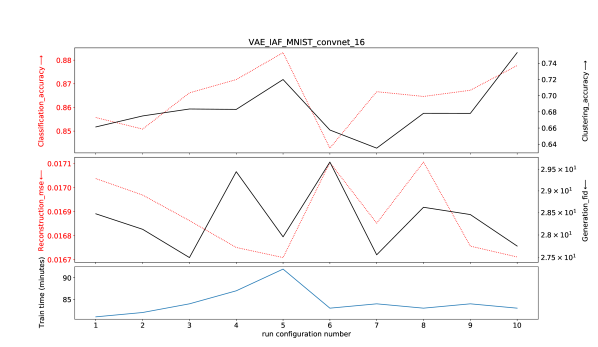
$\beta$-VAE

Higgins et al. [30] argue that increasing the weight of the KL divergence term in the ELBO loss enforces a stronger disentanglement of the latent features as the posterior probability is forced to match a multivariate standard Gaussian. They propose to add a hyper-parameter $\beta$ in the ELBO leading to the following objective to maximise:

$$\mathcal{L}_{\beta\text{-VAE}}(x)=\mathbb{E}_{z\sim q_{\phi}}[\log p_{\theta}(x|z)]-\beta\mathcal{D}_{KL}\big{[}q_{\phi}(z|x)||p_{z}(z)\big{]}\,.$$

Although the original publication specifies $\beta>1$ to encourage a better disentanglement, a smaller value of $\beta$ can be used to relax the regularisation constraint of the VAE. Therefore, for this model we consider a range of values for $\beta$ from $1e^{-3}$ to $1e^{3}$.

As expected, we see in Fig. 19 a trade-off appearing between reconstruction and generation. Indeed, a very small $\beta$ will tend to less regularise the model since the latent variables will no longer be driven to follow the prior, favouring a better reconstruction. On the other hand, a higher value for $\beta$ will constrain the model, leading to a better generation quality. Moreover, as can be seen in Fig. 19, too high a value of $\beta$ will lead to over-regularisation, resulting in poor performances on all evaluated tasks.

Results by configuration

Table 12: $\beta$-VAE configurations

Config	1	2	3	4	5	6	7	8	9	10
$\beta$	$1e^{-3}$	$1e^{-2}$	$1e^{-1}$	$0.5$	2	5	10	20	$1e^{2}$	$1e^{3}$

Figure 19: Results on $\beta$-VAE

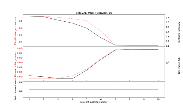
$\beta$-TC-VAE

Chen et al. [16] extend on the ideas of Higgins et al. [30] by rewriting and re-weighting specific terms in the ELBO loss with multiple hyperparameters. The authors note that the KL-divergence term of the ELBO loss can be rewritten as

$$\mathbb{E}_{x\sim p_{\theta}}\bigg{[}\mathcal{D}_{KL}\big{[}q_{\phi}(z|x)||p_{z}(z)\big{]}\bigg{]}=\underbrace{I(x,z)}_{\text{Mutual information}} +\underbrace{\mathcal{D}_{KL}\big{[}q_{\phi}(z)||\prod_{j=1}^{d}q_{\phi}(z_{j})\big{]}}_{\text{TC-loss}}$$

$$+\underbrace{\sum_{j=1}^{d}\mathcal{D}_{KL}\big{[}q_{\phi}(z_{j})||p_{z}(z_{j})\big{]}}_{\text{Dimension-wise KL}}$$

• The mutual information term corresponds to the amount of information shared by $x$ and its latent representation $z$. It is claimed that maximising the mutual information encourages better disentanglement and a more compact representation of the data.

• The TC-loss corresponds to the total correlation between the latent distribution and its fully disentangled version, maximising it enforces the dimensions of the latent vector to be uncorrelated.

• Maximising the dimension-wise KL prevents the marginal distribution of each latent dimension from diverging too far from the prior Gaussian distribution

The authors therefore propose to replace the classical regularisation term with the more general term

$$\mathcal{L}_{\text{reg}}:=\alpha I(x,n)+\beta\mathcal{D}_{KL}\big{[}q_{\phi}(z)||\prod_{j}q_{\phi}(z_{j})\big{]}+\gamma\sum_{j}\mathcal{D}_{KL}\big{[}q_{\phi}(z_{j})||p_{z}(z_{j})\big{]}\,.$$

Similarly to the authors, we set $\alpha=\gamma=1$ and only perform a search on the parameter $\beta$. Fig. 20 shows a reconstruction-generation trade-off similar to the $\beta$-VAE model

Results by configuration

Table 13: $\beta$-TC-VAE configurations

Config	1	2	3	4	5	6	7	8	9	10
$\beta$	$1e^{-3}$	$1e^{-2}$	$1e^{-1}$	$0.5$	1	2	5	10	50	$1e^{2}$

Figure 20: Results on $\beta$-TC-VAE

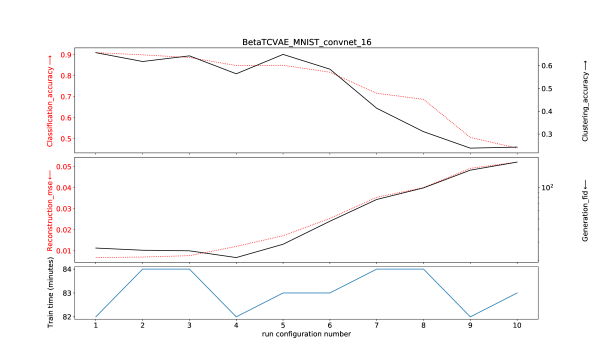
Factor VAE

Kim and Mnih [35] augment the VAE objective with a penalty that encourages factorial representation of the marginal distributions, enforcing a stronger disentangling of the latent space. Noting that a high $\beta$ value in $\beta$-VAE ELBO loss encourages disentanglement at the expense of reconstruction quality, FactorVAE proposes a new lower bound of the log likelihood with an added disentanglement term:

$$\mathcal{L}_{\text{FactorVAE}}(x):=\mathcal{L}_{ELBO}(x)-\gamma\mathcal{D}_{KL}\big{(}q_{\phi}(z)||\bar{q}_{\phi}(z)\big{)}\ \text{, with }\bar{q}_{\phi}(z):=\prod_{j=1}^{d}q_{\phi}(z_{j})$$

The distribution of representations $q_{\phi}(z)=\frac{1}{N}\sum_{i=1}^{N}q_{\phi}(z|x_{i})$ of the entire dataset is therefore forced to be close to its fully-disentangled equivalent $\bar{q}_{\phi}(z)$ while leaving the ELBO loss as it is. They further propose to approximate the KL divergence with a discriminator network $D$ that is trained jointly to the VAE:

$$\mathcal{D}_{KL}\big{(}q(z)||\bar{q}(z)\big{)}\approx\mathbb{E}_{q_{z}(z)}\bigg{[}\log\frac{D(z)}{1-D(z)}\bigg{]}$$

As suggested in the authors’s paper, the discriminator is set as a MLP composed of 6 layers each with 1000 hidden units and LeakyReLU activation.

Results by configuration

Table 14: FactorVAE configurations

Config	1	2	3	4	5	6	7	8	9	10
$\gamma$	1	2	5	10	15	20	30	40	50	100

Figure 21: Results on FactorVAE

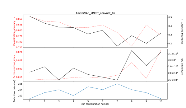
InfoVAE

Zhao et al. [72] note that the traditional VAE ELBO objective can lead to both inaccurate amortized inference and VAE models that tend to ignore most of the latent variables, therefore not fully taking advantage of the modelling capacities of the VAE scheme and learning less meaningful latent representations. In order to counteract these two issues, they propose to rewrite and re-weight the ELBO objective in order to counterbalance the imbalance between the distribution in the data space and the latent space, and add a mutual information term between $x$ and $z$ to encourage a stronger dependency between the two variables, preventing the model from ignoring the latent encoding. One can re-write the ELBO loss in order to explicit the KL divergence between the marginalised posterior and the prior

$$\mathcal{L}_{\text{ELBO}}(x):=-\mathcal{D}_{KL}[q_{\phi}(z)||p_{z}(z)]-\mathbb{E}_{z\sim p_{z}}\bigg{[}\mathcal{D}_{KL}[q_{\phi}(x|z)||p_{\theta}(x|z)]\bigg{]}\,.$$

Introducing an additional mutual information term $I_{q}(x;z)$ and extending the objective function to use any given divergence $D$ between probability measures instead of the KL objective, the authors propose a new objective defined as

$$\mathcal{L}_{\text{InfoVAE}}(x):=-\lambda D[q_{\phi}(z)||p_{z}(z)]-\mathbb{E}_{z\sim p_{z}}\bigg{[}\mathcal{D}_{KL}[q_{\phi}(x|z)||p_{\theta}(x|z)]\bigg{]}+\alpha I_{q}(x;z)$$

where $\lambda$ and $\alpha$ are hyperparameters. In our experiments, $\alpha$ is set to 0 as recommended in the paper in the case where $p_{\theta}(x|z)$ is a simple distribution. $D$ is chosen as the Maximum Mean Discrepancy (MMD) [28], defined as

$$\mbox{MMD}_{k}(p_{\lambda}(z),q_{\phi}(z))=||\int_{\mathcal{Z}}k(z,.)dp_{\lambda}(z)-\int_{\mathcal{Z}}k(z,.)dq_{\phi}(z)||_{\mathcal{H}_{k}}$$

with $k:\mathcal{Z}\times\mathcal{Z}\rightarrow\mathbb{R}$ a positive-definite kernel and its associated RKHS $\mathcal{H}_{k}$. We choose to differentiate 2 cases in the benchmark: one with a Radial Basis Function (RBF) kernel, the other with the Inverse MultiQuadratic (IMQ) kernel as proposed in [64] where the kernel is given by $k(x,y)=\sum\limits_{s\in\mathcal{S}}\frac{s\cdot C}{s\cdot C+\|x-y\|_{2}^{2}}$ with $s\in[0.1,0.2,0.5,1,2,5,10]$ and $C=2\cdot d\cdot\sigma^{2}$, $d$ being the dimension of the latent space and $\sigma$ a parameter part of the hyper-parameter search.

The authors underline that choosing $\lambda>0$, $\alpha=1-\lambda$ and $D=\mathcal{D}_{KL}$, we recover the $\beta$-VAE model [30], while choosing $\alpha=\lambda=1$ and setting $D$ as the Jensen Shannon divergence we recover the Adversarial AE model [44].

Results by configuration

Table 15: InfoVAE configurations

Config	1	2	3	4	5	6	7	8	9	10
kernel bandwidth - $\sigma$	$1e^{-2}$	$1e^{-1}$	0.5	1	1	1	1	1	2	5
$\lambda$	10	10	10	$1e^{-2}$	$1e^{-1}$	10	100	100	10	10

Figure 22: Results on InfoVAE-RBF

Figure 23: Results on InfoVAE-IMQ

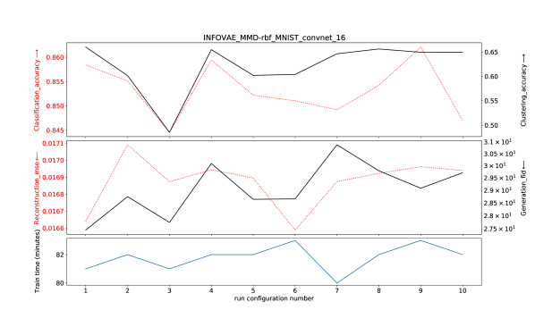
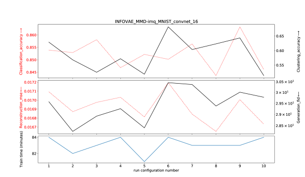
Adversarial AE (AAE)

Makhzani [44] propose to use a GAN-like approach by replacing the regularisation induced by the KL divergence with a discriminator network $D$ trained to differentiate between samples from the prior and samples from the posterior distribution. The encoder network therefore acts as a generator network, leading to the following objective

$$\mathcal{L}_{\text{AAE}}(x)=\mathbb{E}_{z\sim q_{\phi}(z|x)}[\log p_{\theta}(x|z)]+\alpha\mathcal{L}_{\mathrm{GAN}}\,,$$

with $\mathcal{L}_{\mathrm{GAN}}$ the standard GAN loss defined by

$$\mathcal{L}_{\mathrm{GAN}}=\mathbb{E}_{\tilde{z}\sim p_{z}(z)}\bigg{[}\log(1-D(\tilde{z})))\bigg{]}+\mathbb{E}_{x\sim p_{\theta}}\bigg{[}\mathbb{E}_{z\sim q_{\phi}(z|x)}[\log D(z)]\bigg{]}\,.$$

For the Adversarial Autoencoder implementation, we use a MLP neural network for the discriminator composed of a single hidden layer with 256 units and ReLU activation.

We observe a similar trade-off between reconstruction and generation quality as observed with $\beta$-VAE type models, as the $\alpha$ term acts like the $\beta$ term, balancing between regularisation and reconstruction.

Results by configuration

Table 16: AAE configurations

Config	1	2	3	4	5	6	7	8	9	10
$\alpha$	$1e^{-3}$	$1e^{-2}$	$1e^{-1}$	0.25	0.5	0.75	0.9	0.95	0.99	0.999

Figure 24: Results on Adversarial AE

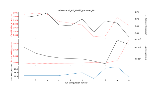
EL-VAE (MSSSIM-VAE)

Snell et al. [61] propose an extension of the ELBO loss to a more general case where any deterministic reconstruction loss $\Delta(x,\hat{x})$ can be used by replacing the probabilistic decoder $p_{\theta}$ with a deterministic equivalent $f_{\theta}$ such that the reconstruction $\hat{x}$ of $x$ given $z\sim q_{\phi}(z|x)$ is defined as $\hat{x}=f_{\theta}(z)$. The modified ELBO objective is thus defined as

$$\mathcal{L}_{\mathrm{EL-VAE}}(x)=\Delta(x,\hat{x})-\beta\mathcal{D}_{KL}\big{(}q_{\phi}(z|x)||p(z)\big{)}\,,$$

with $\beta\leq 1$. As suggested in the original paper we use a multi scale variant of the single scale SSIM [68]: the Multi Scale Structural Similarity Metric (MS-SSIM) [67].

Results by configuration

Table 17: MSSSIM-VAE configurations

Config	1	2	3	4	5	6	7	8	9	10
$\beta$	$1e^{-2}$	$1e^{-2}$	$1e^{-2}$	$1e^{-1}$	$1e^{-1}$	$1e^{-1}$	1	1	1	1
window size in MSSSIM	3	5	11	5	3	11	11	5	3	15

Figure 25: Results on MSSSIM-VAE

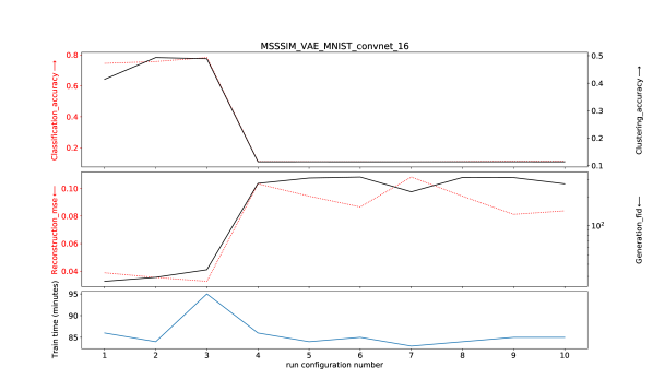
VAE-GAN

Larsen et al. [41] use a GAN like approach by training a discriminator to distinguish real data from reconstructed data. In addition, the discriminator learns to distinguish between real data and data generated by sampling from the prior distribution in the latent space.

Noting that intermediate layers of a discriminative network trained to differentiate real from generated data can act as data-specific features, the authors propose to replace the reconstruction loss of the ELBO with a Gaussian log-likelihood between outputs of intermediate layers of a discriminative network $D$:

$$\mathcal{L}_{\text{VAE-GAN}}=\underbrace{\mathbb{E}_{z\sim q_{\theta}(z|x)}\bigg{[}\log\mathcal{N}(D_{l}(x)|D_{l}(\hat{x}),I)\bigg{]}}_{\text{reconstruction}}-\underbrace{\mathcal{D}_{KL}\big{[}q_{\phi}(z|x)||p_{z}(z)\big{]}}_{\text{regularisation}}-\mathcal{L}_{GAN}\,,$$

where $D_{l}$ is the output of the $l^{\mathrm{th}}$ layer of the discriminator $D$, chosen to be representative of abstract intermediate features learned by the discriminator, and $\mathcal{L}_{\mathrm{GAN}}$ is the standard GAN objective defined as

$$\mathcal{L}_{\mathrm{GAN}}=\log\bigg{(}\frac{D(x)}{1-D(x_{\mathrm{gen}})}\bigg{)}\,,$$

where $x_{\mathrm{gen}}$ is generated using $z\sim p_{z}(z)$. As encouraged by the authors, we add a hyper-parameter $\alpha$ to the reconstruction loss for the decoder only, such that a higher value of $\alpha$ will encourage better reconstruction abilities with respect to the features extracted at the $l^{\mathrm{th}}$ layer of the discriminator network, whereas a smaller value will encourage fooling the discriminator, therefore favouring regularisation toward the prior distribution. For the VAEGAN implementation, we use a discriminator whose architecture is similar to the model’s encoder given in Table. 5. For MNIST and CIFAR we remove the BatchNorm layer and change the activation of layer 2 to Tanh instead of ReLU. For CELEBA, the BatchNorm layer is kept and the activation of layer 2 is also changed to Tanh. For all datasets, the output size of the last linear layer is set to 1 instead of $d$ and followed by a Sigmoid activation.

Results by configuration

Table 18: VAEGAN configurations

Config	1	2	3	4	5	6	7	8	9	10
$\alpha$	0.3	0.5	0.7	0.8	0.8	0.8	0.9	0.9	0.99	0.999
reconstruction layer (l)	3	3	3	3	2	4	3	3	3	3

Figure 26: Results on VAEGAN

Wasserstein Autoencoder (WAE)

Tolstikhin et al. [64] generalise the VAE objective by replacing both terms in the ELBO: similarly to [61] (EL-VAE), the reconstruction loss is replaced by any measurable cost function $\Delta$, and the standard KL divergence is substituted with any arbitrary divergence $\mathcal{D}$ between two distributions, leading to the following objective function

$$E_{q_{\phi}(z|x)}[\Delta(x,\hat{x})]+\lambda\mathcal{D}_{z}(p_{z}(z),q_{\phi}(z))\,,$$

with $\lambda$ a hyper-parameter. The authors propose two different penalties for $\mathcal{D}_{z}$:

1. GAN-based: WAE-GAN

   An adversarial discriminatory network $D(z,z^{\prime})$ is trained jointly to separate the "true" points sampled from the prior $p_{z}(z)$ from the "fake" ones sampled from $q_{\phi}(z|x)$, similarly to [44] (Adversarial AE).

2. MMD-based

   The Maximum Mean Discrepancy is used as a distance between the prior and the posterior distribution. This is the case considered in the benchmark. We choose to differentiate 2 cases in the benchmark: one with a Radial Basis Function (RBF) kernel, the other with the Inverse MultiQuadratic (IMQ) kernel as proposed in [64] where the kernel is given by $k(x,y)=\sum\limits_{s\in\mathcal{S}}\frac{s\cdot C}{s\cdot C+\|x-y\|_{2}^{2}}$ with $s\in[0.1,0.2,0.5,1,2,5,10]$ and $C=2\cdot d\cdot\sigma^{2}$, $d$ being the dimension of the latent space and $\sigma$ a parameter part of the hyper-parameter search. As proposed by the authors, for this model we choose to use a deterministic encoder meaning that $q_{\phi}(z|x)=\delta_{\mu_{\phi}(x)}$.

Results by configuration

Table 19: WAE configurations

Config	1	2	3	4	5	6	7	8	9	10
kernel bandwidth - $\sigma$	$1e^{-2}$	$1e^{-1}$	0.5	1	1	1	1	1	2	5
$\lambda$	1	1	1	$1e^{-2}$	$1e^{-1}$	1	10	100	1	1

Figure 27: Results on WAE-RBF

Figure 28: Results on WAE-IMQ

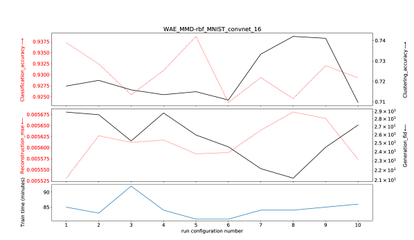
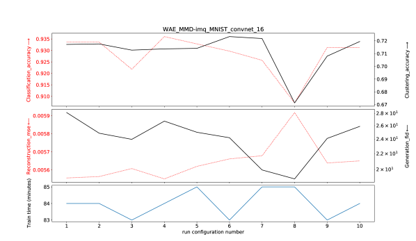
Vector Quantized VAE (VQ-VAE)

Van Den Oord et al. [66] propose to use a discrete space. Therefore, the latent embedding space is defined as a $\mathbb{R}^{K\times D}$ vector space of $K$ different $D$ dimensional embedding vectors $\mathcal{E}=\{e_{1},\dots,e_{K}\}$ which are learned and updated at each iteration.

Given an embedding size $d$ and an input $x$, the output of the encoder $z_{e}(x)$ is of size $\mathbb{R}^{d\times D}$. Each of its $d$ elements is then assigned to the closest embedding vector resulting in an embedded encoding $z_{q}(x)\in\mathcal{E}^{d}$ such that $\big{(}z_{q}(x)\big{)}_{j}=e_{l}$ where $l=\text{argmin}_{1\leq l\leq d}||(z_{e}(x))_{j}-e_{l}||_{2}$ for $j\in[1,d]$. Since the argmin operation is not differentiable, learning of the embeddings and regularisation of the latent space is done by introducing the stopgradient operator $sg$ in the training objective:

$$\mathcal{L}_{\text{VQ-VAE}}(x):=\log p(x|z_{q}(x))+\alpha||sg[z_{e}(x)]-e||_{2}^{2}+\beta||z_{e}(x)-sg[e]||_{2}^{2}\,.$$

For the VQVAE implementation we use the Exponential Moving Average update as proposed in [66] to replace the term $||sg[z_{e}(x)]-e||_{2}^{2}$ in the loss. Thus, we consider only two hyper-parameters in the search: the size of the dictionary of embeddings $K$ and the regularisation factor $\beta$.

Results by configuration

Table 20: VQVAE configurations

Config	1	2	3	4	5	6	7	8	9	10
$K$	128	256	512	512	512	512	512	512	1024	2948
$\beta$	0.25	0.25	0.9	0.1	0.5	0.25	0.75	0.25	0.25	0.25

Figure 29: Results on VQVAE

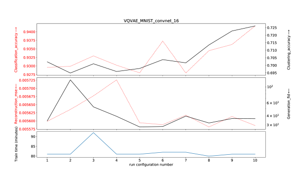
RAE L2 and RAE GP

Ghosh et al. [27] propose to replace the stochastic VAE with a deterministic autoencoder by adapting the ELBO objective to a deterministic case. Under standard VAE assumption with Gaussian decoder, both the reconstruction and the regularisation terms in the ELBO loss can be written in closed form as

$$\left\{\begin{aligned} \mathcal{L}_{\text{reconstruction}}(x)&=||x-\hat{x}||_{2}^{2}\,,\\ \mathcal{L}_{\text{regularisation}}(x)&=\frac{1}{2}\Big{[}||z||^{2}_{2}-d+\sum_{i=1}^{d}(\sigma_{\phi}(x)_{i}-\log\sigma_{\phi}(x)_{i})\Big{]}\,.\end{aligned}\right.$$

Arguing that the regularisation of the VAE model is done through a noise injection mechanism by sampling from the approximate posterior distribution $z\sim\mathcal{N}(\mu_{\phi},diag(\sigma_{\phi}))$, the authors propose to replace this stochastic regularisation with an explicit regularisation term, leading to the following deterministic objective:

$$\mathcal{L}_{\text{RAE}}=||x-\hat{x}||_{2}^{2}+\frac{\beta}{2}||z||^{2}_{2}+\lambda\mathcal{L}_{\text{REG}}\,,$$ (4)

where $\mathcal{L}_{\text{REG}}$ is an explicit regularisation. They propose to use either

• a L2 loss on the weights of the decoder (RAE-L2), which amounts to applying weight decay on the parameters of the decoder.

• a gradient penalty on the output of the decoder (RAE-GP), which amounts to applying a L2 norm on the gradient of the output of the decoder.

Results by configuration

Table 21: RAE configurations

Config	1	2	3	4	5	6	7	8	9	10
$\beta$	$1e^{-6}$	$1e^{-4}$	$1e^{-3}$	$1e^{-3}$	$1e^{-3}$	$1e^{-3}$	$1e^{-3}$	$1e^{-2}$	$1e^{-1}$	1
$\lambda$	$1e^{-3}$	$1e^{-3}$	$1e^{-6}$	$1e^{-4}$	$1e^{-2}$	$1e^{-1}$	1	$1e^{-3}$	$1e^{-3}$	$1e^{-3}$

Figure 30: Results on RAE-L2

Figure 31: Results on RAE-GP

References

- Alemi et al. [2017] Alexander A Alemi, Ian Fischer, Joshua V Dillon, and Kevin Murphy. Deep variational information bottleneck. In International Conference on Learning Representations, 2017.
- Aneja et al. [2020] Jyoti Aneja, Alexander Schwing, Jan Kautz, and Arash Vahdat. NCP-VAE: Variational autoencoders with noise contrastive priors. arXiv:2010.02917 [cs, stat], 2020.
- Arvanitidis et al. [2018] Georgios Arvanitidis, Lars Kai Hansen, and Sören Hauberg. Latent space oddity: On the curvature of deep generative models. In 6th International Conference on Learning Representations, ICLR 2018, 2018.
- Barratt and Sharma [2018] Shane Barratt and Rishi Sharma. A note on the inception score. arXiv preprint arXiv:1801.01973, 2018.
- Bauer and Mnih [2019a] Matthias Bauer and Andriy Mnih. Resampled priors for variational autoencoders. In The 22nd International Conference on Artificial Intelligence and Statistics, pages 66–75. PMLR, 2019a.
- Bauer and Mnih [2019b] Matthias Bauer and Andriy Mnih. Resampled priors for variational autoencoders. pages 66–75. PMLR, 2019b. ISBN 2640-3498.
- Berthelot* et al. [2019] David Berthelot*, Colin Raffel*, Aurko Roy, and Ian Goodfellow. Understanding and improving interpolation in autoencoders via an adversarial regularizer. In International Conference on Learning Representations, 2019. URL https://openreview.net/forum?id=S1fQSiCcYm.
- Biewald [2020] Lukas Biewald. Experiment tracking with weights and biases, 2020. URL https://www.wandb.com/. Software available from wandb.com.
- Bisong [2019] Ekaba Bisong. Google Colaboratory, pages 59–64. Apress, Berkeley, CA, 2019. ISBN 978-1-4842-4470-8. doi: 10.1007/978-1-4842-4470-8_7. URL https://doi.org/10.1007/978-1-4842-4470-8_7.
- Blaauw and Bonada [2016] Merlijn Blaauw and Jordi Bonada. Modeling and transforming speech using variational autoencoders. Morgan N, editor. Interspeech 2016; 2016 Sep 8-12; San Francisco, CA.[place unknown]: ISCA; 2016. p. 1770-4., 2016. Publisher: International Speech Communication Association (ISCA).
- Burda et al. [2016] Yuri Burda, Roger Grosse, and Ruslan Salakhutdinov. Importance weighted autoencoders. arXiv:1509.00519 [cs, stat], 2016.
- Burgess [2018] Christopher P. et al. Burgess. Understanding disentangling in -vae. arXiv preprint arXiv:1804.03599, 2018.
- Caterini et al. [2018] Anthony L Caterini, Arnaud Doucet, and Dino Sejdinovic. Hamiltonian variational auto-encoder. In Advances in Neural Information Processing Systems, pages 8167–8177, 2018.
- Chadebec et al. [2021] Clément Chadebec, Elina Thibeau-Sutre, Ninon Burgos, and Stéphanie Allassonnière. Data Augmentation in High Dimensional Low Sample Size Setting Using a Geometry-Based Variational Autoencoder. arXiv preprint arXiv:2105.00026, 2021.
- Chen et al. [2018a] Nutan Chen, Alexej Klushyn, Richard Kurle, Xueyan Jiang, Justin Bayer, and Patrick Smagt. Metrics for deep generative models. In International Conference on Artificial Intelligence and Statistics, pages 1540–1550. PMLR, 2018a.
- Chen et al. [2018b] Ricky TQ Chen, Xuechen Li, Roger B Grosse, and David K Duvenaud. Isolating sources of disentanglement in variational autoencoders. Advances in neural information processing systems, 31, 2018b.
- Chen et al. [2016] Xi Chen, Diederik P Kingma, Tim Salimans, Yan Duan, Prafulla Dhariwal, John Schulman, Ilya Sutskever, and Pieter Abbeel. Variational lossy autoencoder. arXiv preprint arXiv:1611.02731, 2016.
- Chong and Forsyth [2020] Min Jin Chong and David Forsyth. Effectively unbiased fid and inception score and where to find them. In Proceedings of the IEEE/CVF conference on computer vision and pattern recognition, pages 6070–6079, 2020.
- Coates et al. [2011] Adam Coates, Andrew Ng, and Honglak Lee. An analysis of single-layer networks in unsupervised feature learning. In Proceedings of the fourteenth international conference on artificial intelligence and statistics, pages 215–223. JMLR Workshop and Conference Proceedings, 2011.
- Connor et al. [2021] Marissa Connor, Gregory Canal, and Christopher Rozell. Variational autoencoder with learned latent structure. In International Conference on Artificial Intelligence and Statistics, pages 2359–2367. PMLR, 2021.
- Cremer et al. [2018] Chris Cremer, Xuechen Li, and David Duvenaud. Inference suboptimality in variational autoencoders. In International Conference on Machine Learning, pages 1078–1086. PMLR, 2018.
- Dai and Wipf [2018] Bin Dai and David Wipf. Diagnosing and Enhancing VAE Models. In International Conference on Learning Representations, 2018.
- Davidson et al. [2018] Tim R Davidson, Luca Falorsi, Nicola De Cao, Thomas Kipf, and Jakub M Tomczak. Hyperspherical variational auto-encoders. In 34th Conference on Uncertainty in Artificial Intelligence 2018, UAI 2018, pages 856–865. Association For Uncertainty in Artificial Intelligence (AUAI), 2018.
- Dilokthanakul et al. [2017] Nat Dilokthanakul, Pedro A. M. Mediano, Marta Garnelo, Matthew C. H. Lee, Hugh Salimbeni, Kai Arulkumaran, and Murray Shanahan. Deep unsupervised clustering with gaussian mixture variational autoencoders. arXiv:1611.02648 [cs, stat], 2017.
- Falorsi et al. [2018] Luca Falorsi, Pim de Haan, Tim R. Davidson, Nicola De Cao, Maurice Weiler, Patrick Forré, and Taco S. Cohen. Explorations in homeomorphic variational auto-encoding. arXiv:1807.04689 [cs, stat], 2018.
- Germain et al. [2015] Mathieu Germain, Karol Gregor, Iain Murray, and Hugo Larochelle. Made: Masked autoencoder for distribution estimation. In International Conference on Machine Learning, pages 881–889. PMLR, 2015.
- Ghosh et al. [2020] Partha Ghosh, Mehdi SM Sajjadi, Antonio Vergari, Michael Black, and Bernhard Schölkopf. From variational to deterministic autoencoders. In 8th International Conference on Learning Representations, ICLR 2020, 2020.
- Gretton et al. [2012] Arthur Gretton, Karsten M Borgwardt, Malte J Rasch, Bernhard Schölkopf, and Alexander Smola. A kernel two-sample test. The Journal of Machine Learning Research, 13(1):723–773, 2012.
- Heusel et al. [2017] Martin Heusel, Hubert Ramsauer, Thomas Unterthiner, Bernhard Nessler, and Sepp Hochreiter. Gans trained by a two time-scale update rule converge to a local nash equilibrium. In Advances in Neural Information Processing Systems, 2017.
- Higgins et al. [2017] Irina Higgins, Loic Matthey, Arka Pal, Christopher Burgess, Xavier Glorot, Matthew Botvinick, Shakir Mohamed, and Alexander Lerchner. beta-VAE: Learning basic visual concepts with a constrained variational framework. ICLR, 2(5):6, 2017.
- Hoffman and Johnson [2016] Matthew D Hoffman and Matthew J Johnson. Elbo surgery: yet another way to carve up the variational evidence lower bound. In Workshop in Advances in Approximate Bayesian Inference, NIPS, volume 1, page 2, 2016.
- Jordan et al. [1999] Michael I Jordan, Zoubin Ghahramani, Tommi S Jaakkola, and Lawrence K Saul. An introduction to variational methods for graphical models. Machine Learning, 37(2):183–233, 1999.
- Jung and Keuper [2021] Steffen Jung and Margret Keuper. Internalized biases in fréchet inception distance. In NeurIPS 2021 Workshop on Distribution Shifts: Connecting Methods and Applications, 2021.
- Kalatzis et al. [2020] Dimitrios Kalatzis, David Eklund, Georgios Arvanitidis, and Soren Hauberg. Variational autoencoders with riemannian brownian motion priors. In International Conference on Machine Learning, pages 5053–5066. PMLR, 2020.
- Kim and Mnih [2018] Hyunjik Kim and Andriy Mnih. Disentangling by factorising. In International Conference on Machine Learning, pages 2649–2658. PMLR, 2018.
- Kingma and Ba [2014] Diederik P Kingma and Jimmy Ba. Adam: A method for stochastic optimization. arXiv preprint arXiv:1412.6980, 2014.
- Kingma and Welling [2014] Diederik P. Kingma and Max Welling. Auto-encoding variational bayes. arXiv:1312.6114 [cs, stat], 2014.
- Kingma et al. [2016] Durk P. Kingma, Tim Salimans, Rafal Jozefowicz, Xi Chen, Ilya Sutskever, and Max Welling. Improved variational inference with inverse autoregressive flow. Advances in neural information processing systems, 29, 2016.
- Klushyn et al. [2019] Alexej Klushyn, Nutan Chen, Richard Kurle, and Botond Cseke. Learning Hierarchical Priors in VAEs. Advances in neural information processing systems, page 10, 2019.
- Krizhevsky et al. [2009] Alex Krizhevsky, Geoffrey Hinton, et al. Learning multiple layers of features from tiny images. 2009.
- Larsen et al. [2016] Anders Boesen Lindbo Larsen, Søren Kaae Sønderby, Hugo Larochelle, and Ole Winther. Autoencoding beyond pixels using a learned similarity metric. In International conference on machine learning, pages 1558–1566. PMLR, 2016.
- LeCun [1998] Yann LeCun. The MNIST database of handwritten digits. 1998.
- Liu et al. [2015] Ziwei Liu, Ping Luo, Xiaogang Wang, and Xiaoou Tang. Deep learning face attributes in the wild. In Proceedings of International Conference on Computer Vision (ICCV), December 2015.
- Makhzani [2016] Alireza et al. Makhzani. Adversarial autoencoders. arXiv preprint arXiv:1511.05644, 2016.
- Mathieu et al. [2019a] Emile Mathieu, Charline Le Lan, Chris J Maddison, Ryota Tomioka, and Yee Whye Teh. Continuous hierarchical representations with poincaré variational auto-encoders. In Advances in neural information processing systems, pages 12565–12576, 2019a.
- Mathieu et al. [2019b] Emile Mathieu, Tom Rainforth, Nana Siddharth, and Yee Whye Teh. Disentangling disentanglement in variational autoencoders. In International Conference on Machine Learning, pages 4402–4412. PMLR, 2019b.
- Morozov et al. [2020] Stanislav Morozov, Andrey Voynov, and Artem Babenko. On self-supervised image representations for gan evaluation. In International Conference on Learning Representations, 2020.
- Nalisnick et al. [2016] Eric Nalisnick, Lars Hertel, and Padhraic Smyth. Approximate inference for deep latent gaussian mixtures. In NIPS Workshop on Bayesian Deep Learning, volume 2, page 131, 2016.
- Neal [2005] Radford M Neal. Hamiltonian importance sampling. In talk presented at the Banff International Research Station (BIRS) workshop on Mathematical Issues in Molecular Dynamics, 2005.
- Pang et al. [2020] Bo Pang, Tian Han, Erik Nijkamp, Song-Chun Zhu, and Ying Nian Wu. Learning latent space energy-based prior model. Advances in Neural Information Processing Systems, 33, 2020.
- Papamakarios et al. [2017] George Papamakarios, Theo Pavlakou, and Iain Murray. Masked autoregressive flow for density estimation. Advances in neural information processing systems, 30, 2017.
- Paszke et al. [2017] Adam Paszke, Sam Gross, Soumith Chintala, Gregory Chanan, Edward Yang, Zachary DeVito, Zeming Lin, Alban Desmaison, Luca Antiga, and Adam Lerer. Automatic differentiation in pytorch. 2017.
- Pedregosa et al. [2011] F. Pedregosa, G. Varoquaux, A. Gramfort, V. Michel, B. Thirion, O. Grisel, M. Blondel, P. Prettenhofer, R. Weiss, V. Dubourg, J. Vanderplas, A. Passos, D. Cournapeau, M. Brucher, M. Perrot, and E. Duchesnay. Scikit-learn: Machine learning in python. Journal of Machine Learning Research, 12:2825–2830, 2011.
- Razavi et al. [2020] Ali Razavi, Aaron van den Oord, and Oriol Vinyals. Generating diverse high-fidelity images with vq-vae-2. Advances in Neural Information Processing Systems, 2020.
- Rezende and Mohamed [2015] Danilo Rezende and Shakir Mohamed. Variational inference with normalizing flows. In International Conference on Machine Learning, pages 1530–1538. PMLR, 2015.
- Rezende et al. [2014] Danilo Jimenez Rezende, Shakir Mohamed, and Daan Wierstra. Stochastic backpropagation and approximate inference in deep generative models. In International conference on machine learning, pages 1278–1286. PMLR, 2014.
- Salimans et al. [2015] Tim Salimans, Diederik Kingma, and Max Welling. Markov chain monte carlo and variational inference: Bridging the gap. In International Conference on Machine Learning, pages 1218–1226, 2015.
- Salimans et al. [2016] Tim Salimans, Ian Goodfellow, Wojciech Zaremba, Vicki Cheung, Alec Radford, and Xi Chen. Improved techniques for training gans. Advances in neural information processing systems, 29, 2016.
- Shao et al. [2018] Hang Shao, Abhishek Kumar, and P. Thomas Fletcher. The riemannian geometry of deep generative models. In 2018 IEEE/CVF Conference on Computer Vision and Pattern Recognition Workshops (CVPRW), pages 428–4288. IEEE, 2018. ISBN 978-1-5386-6100-0. doi: 10.1109/CVPRW.2018.00071.
- Shmelkov et al. [2018] Konstantin Shmelkov, Cordelia Schmid, and Karteek Alahari. How good is my gan? In Proceedings of the European Conference on Computer Vision (ECCV), pages 213–229, 2018.
- Snell et al. [2017] Jake Snell, Karl Ridgeway, Renjie Liao, Brett D Roads, Michael C Mozer, and Richard S Zemel. Learning to generate images with perceptual similarity metrics. In 2017 IEEE International Conference on Image Processing (ICIP), pages 4277–4281. IEEE, 2017.
- Sønderby et al. [2016] Casper Kaae Sønderby, Tapani Raiko, Lars Maaløe, Søren Kaae Sønderby, and Ole Winther. Ladder variational autoencoder. In 29th Annual Conference on Neural Information Processing Systems (NIPS 2016), 2016.
- Subramanian [2020] A.K Subramanian. Pytorch-vae. https://github.com/AntixK/PyTorch-VAE, 2020.
- Tolstikhin et al. [2018] I Tolstikhin, O Bousquet, S Gelly, and B Schölkopf. Wasserstein auto-encoders. In 6th International Conference on Learning Representations (ICLR 2018), 2018.
- Tomczak and Welling [2018] Jakub Tomczak and Max Welling. Vae with a vampprior. In International Conference on Artificial Intelligence and Statistics, pages 1214–1223. PMLR, 2018.
- Van Den Oord et al. [2017] Aaron Van Den Oord, Oriol Vinyals, et al. Neural discrete representation learning. Advances in neural information processing systems, 30, 2017.
- Wang et al. [2003] Zhou Wang, Eero P Simoncelli, and Alan C Bovik. Multiscale structural similarity for image quality assessment. In The Thrity-Seventh Asilomar Conference on Signals, Systems & Computers, 2003, volume 2, pages 1398–1402. Ieee, 2003.
- Wang et al. [2004] Zhou Wang, Alan C Bovik, Hamid R Sheikh, and Eero P Simoncelli. Image quality assessment: from error visibility to structural similarity. IEEE transactions on image processing, 13(4):600–612, 2004.
- Wolf et al. [2020] Thomas Wolf, Lysandre Debut, Victor Sanh, Julien Chaumond, Clement Delangue, Anthony Moi, Pierric Cistac, Tim Rault, Rémi Louf, Morgan Funtowicz, Joe Davison, Sam Shleifer, Patrick von Platen, Clara Ma, Yacine Jernite, Julien Plu, Canwen Xu, Teven Le Scao, Sylvain Gugger, Mariama Drame, Quentin Lhoest, and Alexander M. Rush. Transformers: State-of-the-art natural language processing. In Proceedings of the 2020 Conference on Empirical Methods in Natural Language Processing: System Demonstrations, pages 38–45, Online, October 2020. Association for Computational Linguistics. URL https://www.aclweb.org/anthology/2020.emnlp-demos.6.
- Yang et al. [2019] Linxiao Yang, Ngai-Man Cheung, Jiaying Li, and Jun Fang. Deep clustering by gaussian mixture variational autoencoders with graph embedding. In Proceedings of the IEEE/CVF International Conference on Computer Vision, pages 6440–6449, 2019.
- Zhang et al. [2018] Cheng Zhang, Judith Bütepage, Hedvig Kjellström, and Stephan Mandt. Advances in variational inference. IEEE Transactions on Pattern Analysis and Machine Intelligence, 41(8):2008–2026, 2018.
- Zhao et al. [2016] Shengjia Zhao, Jiaming Song, and Stefano Ermon. Infovae: Information maximizing variational autoencoders. arXiv preprint arXiv:1706.02262, 2016.