Warp and flare of the Galactic disc revealed with supergiants by Gaia EDR3
Abstract
Context. The outer Galactic disc contains some features such as the warp and flare, whose origin is still debated. The Gaia data provide an excellent opportunity to probe the Galactic disc at large distances and study these features.
Aims. We derive the density distributions of the average (old) whole population and the supergiants (representative of a young population), and we use them to constrain their warp and flare. By comparing the results, we study how the properties of these phenomena depend on the studied population.
Methods. We used Lucy’s deconvolution method to recover corrected star counts as a function of distance, from which we derive the density distribution.
Results. We find that supergiants have an asymmetric warp, reaching a maximum amplitude of kpc and minimum amplitude of kpc at a distance of kpc, which is almost twice as high as the amplitude of the whole population of the disc. We find a significant flare of the whole population, especially in the thick disc. The scale height increases from kpc and kpc in the solar neighbourhood, to kpc and kpc in the remote regions of the Milky Way ( kpc). The supergiants’ population has only a small flare.
Key Words.:
Galaxy:disc – Galaxy: structure1 Introduction
Although we have an extensive knowledge of our Galaxy, there are still many aspects for which our understanding of the Milky Way is incomplete. Wide discussions about features such as warp, flare, or cut-off show that there is much more to be learned about the Milky Way. To this end, the Gaia Early Data Release 3 (Gaia Collaboration et al. 2021b, EDR3) presents an opportunity to study the Galaxy in greater detail than ever before. With its precise positional, proper motions, radial velocity measurements, and distance determinations for millions of stars, it offers the most accurate information about our Galaxy to date; ideal for making advances in all branches of Galactic astrophysics.
The Galactic warp is a well-known feature of the Galactic disc, but its shape is constrained only roughly and there is no consensus on the mechanism causing it. Some of the theories include accretion of intergalactic matter onto the disc (López-Corredoira et al. 2002a), a misaligned halo (Ostriker & Binney 1989), interaction with satellites (García-Ruiz et al. 2002), or an intergalactic magnetic field (Battaner et al. 1990). Currently the kinematical information about the warp is not sufficient to constrain the formation models. Chrobáková et al. (2020) compared the warp of the whole stellar population with the warp of Cepheids and suggest that warp is dependent on the age of the studied population, which would indicate that warp is caused by a non-gravitational mechanism. A similar conclusion was reached by Wang et al. (2020) using LAMOST DR4. In this paper, we recalculate the Galactic warp using the most recent Gaia EDR3 data and compare this with the warp of supergiants, to test this hypothesis.
The flare is an increase in the scale height of the Galactic disc with galactocentric radius, detected in both the gaseous and stellar components. Grabelsky et al. (1987) and May et al. (1997) confirmed flare in the outer disc by tracing molecular clouds, Sánchez-Salcedo et al. (2008) modelled the flare applying modified Newtonian dynamics (MOND), and Narayan & Jog (2002) treated HI, H2, and stars as gravitationally coupled components of the disc, calculating scale heights for all three components and giving predictions for the flare that matched observations very well. Stellar flare was studied by several authors as well (Alard 2000; López-Corredoira et al. 2002b; Momany et al. 2006). López-Corredoira & Molgó (2014) studied 3D stellar distribution using Sloan Extension for Galactic Understanding and Exploration (SEGUE) data, finding that flare is a prominent feature for Galactocentric distance of kpc. Yusifov (2004) reached a similar conclusion studying pulsars. Bovy et al. (2016b) studied the structure of the Galactic disc, distinguishing various stellar populations using APOGEE survey data covering Galactocentric distances of kpc. They did not find stellar flaring in the high- mono-abundance population, while the low- mono-abundance populations exhibit Galactic flare.
To explain the dependence of the disc thickness on azimuth, Kalberla et al. (2007) modelled it with a ring of dark matter embedded in the disc, and Saha et al. (2009) applied a lopsided dark matter halo. López-Corredoira & Betancort-Rijo (2009) proposed accretion of intergalactic matter onto the disc as a possible mechanism to explain both the flare and its dependence on azimuth.
More recently, the flare was studied with Gaia DR2 using OB stars (Li et al. 2019) or with LAMOST (Wang et al. 2018) and Cepheids (Feast et al. 2014). Possible existence of the flare was also explored in the thick disc (López-Corredoira & Molgó 2014; Mateu & Vivas 2018; Wang et al. 2018). Yu, Y. et al. (2021) studied the warp and the flare traced by OB stars using LAMOST DR5 data and Yu, Z. et al. (2021) investigated the Galactic disc using LAMOST and Gaia Red Clump Sample VII.
In this paper, we use the Gaia EDR3 data to study the warp and flare. We are especially interested in the properties of these features for various stellar populations, and therefore we analyse separately the population of supergiants. The paper is structured as follows. In Section 2 we describe our data selection and the extinction map used. In Section 3 we present the method used to calculate the density distribution and explain how we chose the sample of supergiants. Section 4 is dedicated to the analysis of the warp and Section 5 deals with the analysis of the flare. In Section 6 we conclude the paper.
2 Data Selection
We used the Gaia EDR3 data, collected during the first 34 months of observations. We are interested in sources with G-band (330–1050 nm) magnitude. The photometric uncertainties were mmag for G¡13, 1 mmag at G=17, and 6 mmag at G=20 mag. We chose a magnitude up to G=19, where the catalogue was sufficiently complete (Fabricius et al. 2021). More details on the catalogue validation are available in Fabricius et al. (2021). To ensure the quality of the dataset, we applied several constraints. To select sources with good astrometry, we only chose data with five- and six-parameter solutions, satisfying the following condition on renormalised unit weight error (RUWE):
as suggested by Lindegren et al. (2021). In addition, following Gaia Collaboration et al. (2021a), we applied the following constraint to ensure that the sources had good photometry:
where denotes the colour index, with the band covering the range 330–680 nm and the band covering the range 640–1050 nm, and excess_flux is the BP and RP flux excess, corrected as suggested by Riello et al. (2021). Moreover, we applied:
| phot_g_mean_flux_over_error | ||||
| phot_rp_mean_flux_over_error | ||||
| phot_bp_mean_flux_over_error |
which removed variable stars (Gaia Collaboration et al. 2018). We followed the approach of Chrobáková et al. (2020) and chose data with a parallax in the interval [0,2] mas, and apparent magnitude in the - band between G=12 and G=19. We corrected fluxes for six-point sources as well, as suggested by Riello et al. (2021), using codes listed in the appendix of Gaia Collaboration et al. (2021b). We also added the zero-point correction as found by Lindegren et al. (2021), using the publicly available Python package111https://gitlab.com/icc-ub/public/gaiadr3_zeropoint, which calculates the zero-point as a function of ecliptic latitude, magnitude, and colour.
Extinction map
In order to estimate the extinction, we used the three-dimensional, full-sky extinction map from Bovy et al. (2016a), using the Python package mwdust. This extinction map is a combination of maps of Marshall et al. (2006), Green et al. (2015), and Drimmel et al. (2003), and provides reddening as defined in Schlegel et al. (1998).
In order to convert the interstellar reddening of these maps into , we used the coefficients (Hendy 2018; Rybizki et al. 2018):
| (4) |
3 Methods
We followed the approach of Chrobáková et al. (2020), who used the fundamental equation of stellar statistics (Chandresekhar & Münch 1951) to derive the stellar density:
| (5) |
| (6) | |||||
where are the star counts, is the covered angular surface, is the parallax interval (0.01 mas in our case, which must be added in the equation because we did not use the unit parallax), is the luminosity function in the G filter, is the limiting maximum apparent magnitude, and is the extinction as a function of distance. For the luminosity function, we used the values given in Table 1 of Chrobáková et al. (2020) for the whole population; or we determined it following the same method for some sub-samples.
The density determination required that we measure the star counts as a function of distance. However, it is well known that the parallax error grows with the distance from the observer, preventing the precise determination of distances. Therefore, we could not simply use the observed star counts to calculate the density, as at distances higher that roughly 5 kpc they are biased. In order to recover correct star counts, we applied a statistical deconvolution method developed by López-Corredoira & Sylos-Labini (2019) based on Lucy’s method (Lucy 1974). They express the observed number of stars per parallax as a convolution of the real number of stars with a Gaussian function:
| (7) |
where
| (8) |
For the error , we averaged parallax errors of every bin. More details about the method can be found in Chrobáková et al. (2020).
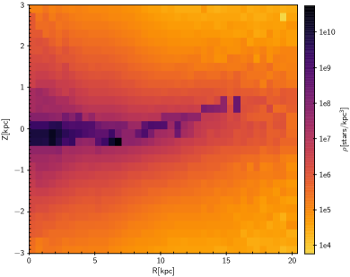
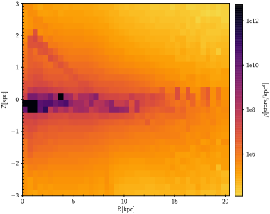
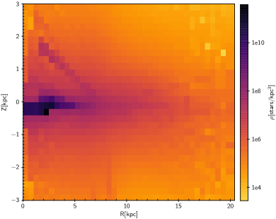
With the corrected star counts, we reveal density distribution up to 20 kpc, which can be seen in Fig. 1. This result is almost identical with the one obtained with Gaia DR2 data (Chrobáková et al. 2020). Similarly, we can see overdensities above the plane for azimuths between and . As commented in Chrobáková et al. (2020), these structures are most likely a contamination, since they disappear after integrating the density through the whole disc.
We divided the data into bins of Galactic longitude , Galactic latitude and apparent magnitude . For the values of , we made bins of length and corresponding in bins of . We divided each of the lines of sight in magnitude, binned with size between G=12 and G=19. We also made bins of mas in parallax. We did not use negative parallaxes because these affect the distribution of parallaxes and statistical properties. However, in our method we do not calculate the average distance from the average parallax. We used Lucy’s method, which iterates the counts of the stars with positive parallaxes, until we obtained the final solution. This does not mean that we truncated the star counts with negative parallaxes; we simply did not use this information because it is not necessary with this approach. Further details on this method and tests of its possible biases can be found in Chrobáková et al. (2020).
4 Sample definition
We analysed this density distribution to reveal the warp and the flare in the whole stellar population, which we will refer to as Sample 0. Moreover, we separated supergiants from the dataset in order to analyse their density distribution separately and find differences with the respect to the whole population. We used two different approaches to separate the supergiants, as described below.
4.1 Sample 1
In the first approach, we chose only stars which we can be certain are supergiants. Based on the error of parallax, we calculated the interval of possible magnitudes in the - band for every star:
| (9) |
where is parallax and is parallax error. Then we chose only the stars with and . In the end we had a dataset of stars.
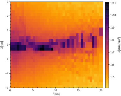
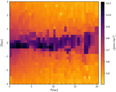
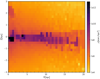
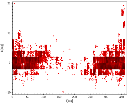
As the distribution was not homogeneous, we divided stars in bins as follows. For and and , we had bins with and . For the same range of for , we had and . We binned the stars in in one bin. We also made bins in magnitude and mas in parallax. In Fig. 2 (a), we show the distribution of the sources selected with this method.
4.2 Sample 2
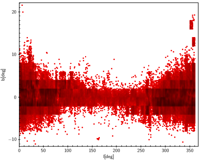
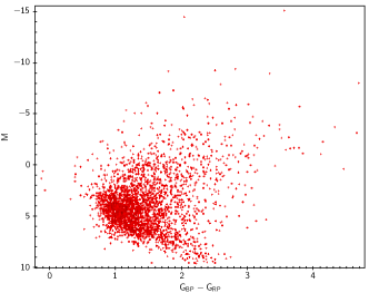
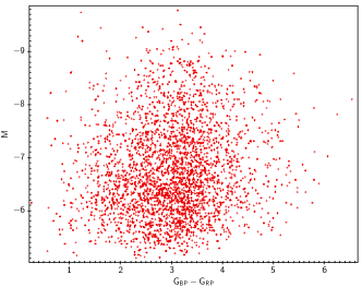
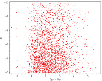
The second approach was less strict; we chose sources with absolute magnitude in the - band within the interval , regardless of the error of the magnitude. The advantage of this method is that we were complete, and therefore we could make statistical analysis of the data to investigate the flare. As this sample was distributed more homogeneously, we divided the stars in bins the same way as for the total population. In Fig. 2 (b), we show the distribution of the sources selected with this method. In the end, this sample contained about stars. In Fig. 3 we show the Hertzsprung-Russell diagrams (HRD) of all three of the samples.
5 Warp analysis
The first feature that we studied is the Galactic warp. We removed data for as in this part we did not have enough data. Following the approach of Chrobáková et al. (2020), we calculated the average elevation of the plane as
| (10) |
Then, we fitted with Eq. (11) of Chrobáková et al. (2020), which represents a common warp model:
| (11) |
where and are free parameters characterizing the warp. We did not account for the height of the Sun on the Galactic plane because some recent studies (e.g. Cheng et al. 2020) suggest that warp starts at smaller radii than previously thought and, therefore, the Solar neighbourhood could be slightly warped. For Sample 0, we find values of warp parameters:
| (12) | |||||
while for Sample 1, we find:
| (13) | |||||
and for Sample 2:
| (14) | |||||
The error of stands for the error of the amplitude alone, without the variations of and . For the fit, we used the function curve fit from the python SciPy package, which uses non-linear least squares to fit a function to data.
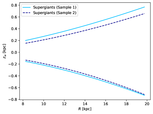
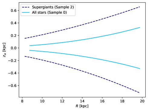
In Fig. 4 we compare the warp amplitude for supergiants for both samples (Sample 1 and Sample 2). The two samples are in very good agreement, yielding warp amplitude with only negligible differences, showing that the Sample 2 is not significantly contaminated. In Fig. 5, we plot the maximum and minimum amplitudes of warp for the whole population (Sample 0), compared with the supergiants (Sample 2). We confirm that the warp amplitude for the whole population is almost identical to what we found with Gaia DR2 data (Chrobáková et al. 2020). We obtain a maximum warp amplitude of kpc and minimum of kpc at a distance of kpc, which is slightly higher than the result obtained with Gaia DR2 data, with a small asymmetry between the northern and the southern warp. From comparison with the supergiants, it is clear that the warp amplitude of supergiants is significantly larger that of the whole population, reaching an amplitude twice as large at a distance of kpc. As supergiants are a young population, a few tens of Myr old on average (e.g. Bouret et al. 2012), whereas the whole population is Gyr old (e.g. Kilic et al. 2017), there is a clear relationship between the warp amplitude and the age of the studied population, thus confirming conclusions of previous studies (Chrobáková et al. 2020; Wang et al. 2020).
6 Flare analysis
In order to investigate the Galactic flare, we considered the density distribution of the Galactic disc as consisting of a thick and a thin component. We adopted the model of the flared disc presented by López-Corredoira & Molgó (2014) in the form:
| (15) | |||||
where the Galactocentric cylindrical coordinate system () is used. This model takes into account the thick and the thin discs, with an exponential decrease in density in the horizontal and the vertical directions. is the scale length of the whole disc. and are the scale heights of the thin and the thick discs, respectively. The deficit of stars in the inner region of the disc is characterised by the parameter (López-Corredoira et al. 2004). Since we focus on the remote regions of the Galaxy, we kept constant at kpc (López-Corredoira & Molgó 2014). The Galactocentric distance of the Sun is kpc and is the volume mass density of the Galactic disc in the solar neighbourhood. The parameter represents the ratio of thick and thin stars in the solar neighbourhood and we kept it at . We experimented with setting as a free parameter, but it was varying only slightly, with negligible influence on , and therefore we kept it at the local value as done by López-Corredoira & Molgó (2014). The parameters , , , and are free and their values were then determined from the fitting procedure. The thin and thick discs were divided based on the geometry of the density profiles in the vertical plane.
| Reference | Data source | Constrains | Scale length [kpc] |
|---|---|---|---|
| This work | Gaia EDR3 | ; the whole population | |
| This work | Gaia EDR3 | ; supergiants (Sample 2) | |
| Chrobáková et al. (2020) | Gaia DR2 | the whole population | |
| Li et al. (2019) | Gaia DR2 | OB stars | |
| Wang et al. (2018) | LAMOST | RGB, thin disc, kpc | |
| Wang et al. (2018) | LAMOST | RGB, thick disc, kpc | |
| López-Corredoira & Molgó (2014) | SDSS-SEGUE | thin disc | |
| López-Corredoira & Molgó (2014) | SDSS-SEGUE | thick disc |
6.1 Method
To find the horizontal and vertical star distribution in the Galactic disc, we used the density maps (Fig. 1). We carried the fitting procedure out in two steps: 1) investigating the density profile in the Galactic equatorial plane; 2) investigating the density profile in the vertical direction.
6.2 Density profile in the Galactic equatorial plane
First of all, we focused on the Galactic plane in order to fit the scale length of the Galactic disc. We applied the following constrains on the data: we used stars with kpc and Galactocentric distances kpc; the bin size was kpc in and kpc in and we only considered bins with number of stars . We applied the disc model with exponential decrease in in the following form:
| (16) | |||||
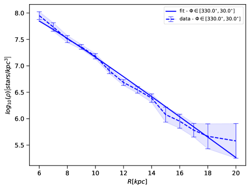
with and as free parameters to be fitted. We defined the azimuthal angle to be measured from the centre-Sun-anticentre direction towards the Galactic rotation, going from to . Since we could not distinguish the individual populations, we neglected the contribution of the thick disc stars in the Galactic equatorial plane. We applied the weighted minimum chi-square method on the data to obtain the values of the fitting parameters in the plane of the Galactic disc given by Eq.(16). The best results of the fitting procedure in the equatorial plane are presented in Table 1, where the comparison with other works is also included. The density profiles in the Galactic plane for the whole data sample are plotted in Fig. 6. Comparing the scale length for various azimuths, one can see the slight dependence of the on , especially for larger Galactic azimuths; kpc and kpc for and for , respectively. On the other hand, variations of the scale length near the centre-Sun-anticentre direction is not present ( kpc and kpc for and for , respectively), and the average value of the scale length kpc (for ) with little dependence on azimuth. The results are in agreement with previous works. For example, Li et al. (2019) present kpc for OB stars using Gaia DR2 data, and Chrobáková et al. (2020) show kpc using Gaia DR2 data. On the other hand, Yu, Y. et al. (2021) show kpc for OB stars.
6.3 The scale height
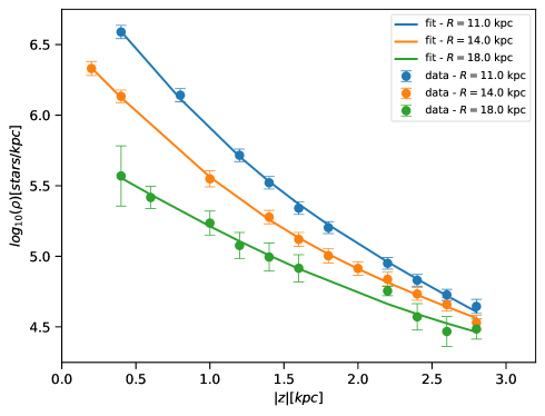
In order to investigate the flaring of the Galactic disc, we fitted the vertical density profiles of the whole data sample, which are presented in Fig. 1, with the model of flared thick and thin discs described by Eq. (6). We applied the weighted minimum chi-square method to obtain the values of the scale height of the thick and thin discs, while the scale length calculated in Sec. 6.2 remained fixed. We divided the data in bins with size kpc and kpc. The vertical density profiles for various values of Galactocentric distances ( kpc, kpc and kpc) are plotted in Fig. 7. The values of the scale height are presented in Table 2 and shown in Fig. 8. The fitting function is a polynomial of the second order. Here, we stress again that we divide the Galactic disc into thin and thick discs, based solely on geometric properties.
| [kpc] | [kpc] | [kpc] |
|---|---|---|
| 5.0 | ||
| 6.0 | ||
| 7.0 | ||
| 8.0 | ||
| 9.0 | ||
| 10.0 | ||
| 11.0 | ||
| 12.0 | ||
| 13.0 | ||
| 14.0 | ||
| 15.0 | ||
| 16.0 | ||
| 17.0 | ||
| 18.0 | ||
| 19.0 | ||
| 20.0 |
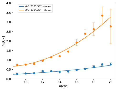
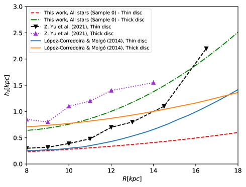
The Galactic flare is significant in Sample 0, which represents the whole population. The scale height of the thin disc rises from kpc in the solar neighbourhood ( kpc) to kpc in the remote regions of the Galactic disc ( kpc). The flaring of the thick disc is even more significant, where the scale height increases from kpc in kpc to reach kpc in kpc. The strong flare in the thick disc is present despite large error bars of for kpc. Comparison of the results with other works is presented in Fig. 9. The flaring of the thin and the thick discs is presented in the results of all authors, but our data exhibits stronger flaring of the thick disc in the remote regions for kpc compared to Yu, Y. et al. (2021) and López-Corredoira & Molgó (2014).
6.4 The northern and southern flare
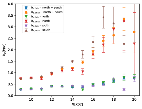
We also focused on the differences between the northern and the southern flare. In Fig. 10 we plot the comparison of the northern, southern and northern+southern flares. There is no significant difference in the dependence of the scale height with the Galactocentric distance for kpc. However, for larger distances, the flaring of the thick disc is asymmetric. The value of the southern scale height is approxomately kpc higher than the of the northern flare in kpc, although the error bars due to the lack of robust datasets in this region have to be taken into account. The difference decreases for kpc and the scale height error bars of the northern and southern flares overlap.
6.5 The azimuthal dependence of the scale height
In order to study the azimuthal dependence of the scale height, we divided the Galactic disc into sectors. We used the following azimuth intervals , , , and . The results for various Galactocentric distances kpc are plotted in Fig. 11.
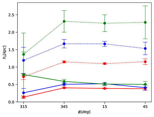
The dependence of the scale height is not significant in our data for kpc. The value of the thick disc in kpc for the azimuth is significantly lower than for the rest of azimuth intervals. However, considering the error bars of , the azimuthal asymmetry almost vanishes.
6.6 Supergiants
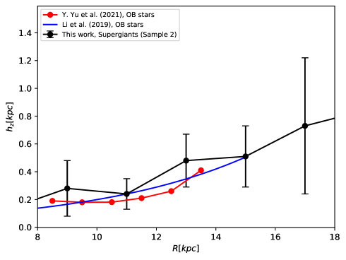
We also investigated the flaring of supergiants. We only used Sample 2, defined in Section 4.2, as Sample 1 was incomplete and therefore could not be used to model the flare. Since we only put constraints on the absolute magnitude of the stars (), contamination is expected in the dataset, although as mentioned is Section 5, it is not significant. We followed the flare analysis procedure described in Sections 6.1 - 6.3. We considered the thin disc and we did not put any constrains on the azimuth. Due to the significantly smaller size of the dataset, we used larger bins: kpc and kpc. We calculated the scale length kpc of the disc. The flaring of Sample 2 stars is presented in Table 3. One can see the subtle increase in , from values kpc in the solar neighbourhood ( kpc) to kpc in the remote regions of the Milky Way ( kpc). A significant increase in the scale height appears for kpc, where kpc. Although the error bars are huge in this interval of the Galactocentric distances (from kpc to kpc), the higher value of the scale height for kpc ( kpc) might be a real feature in the studied data sample. The comparison with other works using OB stars is plotted in Fig. 12.
| R [kpc] | Scale-height [kpc] |
|---|---|
7 Conclusions
We used Gaia EDR3 to study the outer Galactic disc using supergiants and compared them with the whole population. We concentrated on the Galactic warp and flare. The warp of the whole population is similar to the results from previous works (e.g. Chrobáková et al. 2020), reaching a maximum amplitude of kpc and a minimum amplitude of kpc at a distance kpc, revealing a small asymmetry between the northern and the southern warp. The warp of the supergiants, which are notably younger than the whole population, reaches a much larger maximum amplitude of kpc and a minimum of kpc at a distance kpc, with the north-south asymmetry maintained. The difference between the warps of the two populations is significant, confirming a significant relationship between the age of the studied population and the warp amplitude. This result suggests that the warp is induced by a non-gravitational mechanism, such as accretion of intergalactic matter onto the disc or an intergalactic magnetic field.
We find a significant flare of the whole population, especially in the thick disc. The scale height increases from kpc and kpc for kpc, to kpc and kpc at the Galactocentric distance kpc), if the azimuth is considered. We also investigated the dependence of the scale height on the azimuth, which is not present for kpc. For kpc and the changes of the are visible. However, considering the error bars of the , the azimuthal asymmetry almost vanishes. On the other hand, we find a small north-south asymmetry, especially in the thick disc. The asymmetry appears for kpc and the value of of the southern flare is approximately kpc higher than for the northern flare. However, the error bars of the for the northern and the southern flares overlap for kpc. A subtle flare is present in the supergiants population, in comparison with the whole population of the disc. We find a significant increase in the for , but considering error bars, this rise of remains inconclusive. The error bars for reach higher values due to a significant dispersion of densities in vertical profiles and asymmetry between northern and southern flares. It is therefore clear that the population of supergiants is warped more significantly than the whole population, while the flare for this population is less prominent.
Investigation into the warping and flaring mechanisms (e.g. various mechanisms of disc heating, mergers, magnetic field, etc.) is beyond the scope of this study. However, the forthcoming Gaia data releases promise significant improvement in positional and kinematic data, which will pave the way for a better understanding of the dynamics forming these structural features in the remote regions of the Milky Way.
Acknowledgements.
We thank the anonymous referee for helpful comments, which improved this paper. ZC and MLC were supported by the grant PGC-2018-102249-B-100 of the Spanish Ministry of Economy and Competitiveness (MINECO). RN was supported by the VEGA - the Slovak Grant Agency for Science, grant No. 1/0761/21, by the Slovak Research and Development Agency under the contract No. APVV 18-0103 and by the Erasmus+ programe of the European Union under grant No. 2020-1-CZ01-KA203-078200. This work made use of the IAC Supercomputing facility HTCondor (http://research.cs.wisc.edu/htcondor/), partly financed by the Ministry of Economy and Competitiveness with FEDER funds, code IACA13-3E-2493. This work has made use of data from the European Space Agency (ESA) mission Gaia (https://www.cosmos.esa.int/gaia), processed by the Gaia Data Processing and Analysis Consortium (DPAC, https://www.cosmos.esa.int/web/gaia/dpac/consortium). Funding for the DPAC has been provided by national institutions, in particular the institutions participating in the Gaia Multilateral Agreement.References
- Alard (2000) Alard, C. 2000, arXiv e-prints, astro-ph/0007013
- Battaner et al. (1990) Battaner, E., Florido, E., & Sanchez-Saavedra, M. L. 1990, A&A, 236, 1
- Bouret et al. (2012) Bouret, J. C., Hillier, D. J., Lanz, T., & Fullerton, A. W. 2012, A&A, 544, A67
- Bovy et al. (2016a) Bovy, J., Rix, H.-W., Green, G. M., Schlafly, E. F., & Finkbeiner, D. P. 2016a, ApJ, 818, 130
- Bovy et al. (2016b) Bovy, J., Rix, H.-W., Schlafly, E. F., et al. 2016b, ApJ, 823, 30
- Chandresekhar & Münch (1951) Chandresekhar, S. & Münch, G. 1951, ApJ, 113, 150
- Cheng et al. (2020) Cheng, X., Anguiano, B., Majewski, S. R., et al. 2020, ApJ, 905, 49
- Chrobáková et al. (2020) Chrobáková, Ž., Nagy, R., & López-Corredoira, M. 2020, A&A, 637, A96
- Drimmel et al. (2003) Drimmel, R., Cabrera-Lavers, A., & López-Corredoira, M. 2003, A&A, 409, 205
- Fabricius et al. (2021) Fabricius, C., Luri, X., Arenou, F., et al. 2021, A&A, 649, A5
- Feast et al. (2014) Feast, M. W., Menzies, J. W., Matsunaga, N., & Whitelock, P. A. 2014, Nature, 509, 342
- Gaia Collaboration et al. (2021a) Gaia Collaboration, Antoja, T., McMillan, P. J., et al. 2021a, A&A, 649, A8
- Gaia Collaboration et al. (2018) Gaia Collaboration, Babusiaux, C., van Leeuwen, F., et al. 2018, A&A, 616, A10
- Gaia Collaboration et al. (2021b) Gaia Collaboration, Brown, A. G. A., Vallenari, A., et al. 2021b, A&A, 649, A1
- García-Ruiz et al. (2002) García-Ruiz, I., Kuijken, K., & Dubinski, J. 2002, MNRAS, 337, 459
- Grabelsky et al. (1987) Grabelsky, D. A., Cohen, R. S., Bronfman, L., Thaddeus, P., & May, J. 1987, ApJ, 315, 122
- Green et al. (2015) Green, G. M., Schlafly, E. F., Finkbeiner, D. P., et al. 2015, ApJ, 810, 25
- Hendy (2018) Hendy, Y. H. M. 2018, NRIAG Journal of Astronomy and Geophysics, 7, 180
- Kalberla et al. (2007) Kalberla, P. M. W., Dedes, L., Kerp, J., & Haud, U. 2007, A&A, 469, 511
- Kilic et al. (2017) Kilic, M., Munn, J. A., Harris, H. C., et al. 2017, ApJ, 837, 162
- Li et al. (2019) Li, C., Zhao, G., Jia, Y., et al. 2019, ApJ, 871, 208
- Lindegren et al. (2021) Lindegren, L., Bastian, U., Biermann, M., et al. 2021, A&A, 649, A4
- López-Corredoira & Betancort-Rijo (2009) López-Corredoira, M. & Betancort-Rijo, J. 2009, A&A, 493, L9
- López-Corredoira et al. (2002a) López-Corredoira, M., Betancort-Rijo, J., & Beckman, J. E. 2002a, A&A, 386, 169
- López-Corredoira et al. (2002b) López-Corredoira, M., Cabrera-Lavers, A., Garzón, F., & Hammersley, P. L. 2002b, A&A, 394, 883
- López-Corredoira et al. (2004) López-Corredoira, M., Cabrera-Lavers, A., Gerhard, O. E., & Garzón, F. 2004, A&A, 421, 953
- López-Corredoira & Molgó (2014) López-Corredoira, M. & Molgó, J. 2014, A&A, 567, A106
- López-Corredoira & Sylos-Labini (2019) López-Corredoira, M. & Sylos-Labini, F. 2019, A&A, 621, A48
- Lucy (1974) Lucy, L. B. 1974, ApJ, 79, 745
- Marshall et al. (2006) Marshall, D. J., Robin, A. C., Reylé, C., Schultheis, M., & Picaud, S. 2006, A&A, 453, 635
- Mateu & Vivas (2018) Mateu, C. & Vivas, A. K. 2018, MNRAS, 479, 211
- May et al. (1997) May, J., Alvarez, H., & Bronfman, L. 1997, A&A, 327, 325
- Momany et al. (2006) Momany, Y., Zaggia, S., Gilmore, G., et al. 2006, A&A, 451, 515
- Narayan & Jog (2002) Narayan, C. A. & Jog, C. J. 2002, A&A, 394, 89
- Ostriker & Binney (1989) Ostriker, E. C. & Binney, J. J. 1989, MNRAS, 237, 785
- Riello et al. (2021) Riello, M., De Angeli, F., Evans, D. W., et al. 2021, A&A, 649, A3
- Rybizki et al. (2018) Rybizki, J., Demleitner, M., Fouesneau, M., et al. 2018, PASP, 130
- Saha et al. (2009) Saha, K., Levine, E. S., Jog, C. J., & Blitz, L. 2009, ApJ, 697, 2015
- Sánchez-Salcedo et al. (2008) Sánchez-Salcedo, F. J., Saha, K., & Narayan, C. A. 2008, MNRAS, 385, 1585
- Schlegel et al. (1998) Schlegel, D. J., Finkbeiner, D. P., & Davis, M. 1998, ApJ, 500, 525
- Wang et al. (2018) Wang, H.-F., Liu, C., Xu, Y., Wan, J.-C., & Deng, L. 2018, MNRAS, 478, 3367
- Wang et al. (2020) Wang, H. F., López-Corredoira, M., Huang, Y., et al. 2020, ApJ, 897, 119
- Yusifov (2004) Yusifov, I. 2004, in The Magnetized Interstellar Medium, ed. B. Uyaniker, W. Reich, & R. Wielebinski, 165–169
- Yu, Y. et al. (2021) Yu, Y., Wang, H.-F., Cui, W.-Y., et al. 2021, ApJ, 922, 80
- Yu, Z. et al. (2021) Yu, Z., Li, J., Chen, B., et al. 2021, ApJ, 912, 106