Asymptotic Soft Cluster Pruning for Deep Neural Networks
Abstract
Filter pruning method introduces structural sparsity by removing selected filters and is thus particularly effective for reducing complexity. Previous works empirically prune networks from the point of view that filter with smaller norm contributes less to the final results. However, such criteria has been proven sensitive to the distribution of filters, and the accuracy may hard to recover since the capacity gap is fixed once pruned. In this paper, we propose a novel filter pruning method called Asymptotic Soft Cluster Pruning (ASCP), to identify the redundancy of network based on the similarity of filters. Each filter from over-parameterized network is first distinguished by clustering, and then reconstructed to manually introduce redundancy into it. Several guidelines of clustering are proposed to better preserve feature extraction ability. After reconstruction, filters are allowed to be updated to eliminate the effect caused by mistakenly selected. Besides, various decaying strategies of the pruning rate are adopted to stabilize the pruning process and improve the final performance as well. By gradually generating more identical filters within each cluster, ASCP can remove them through channel addition operation with almost no accuracy drop. Extensive experiments on CIFAR-10 and ImageNet datasets show that our method can achieve competitive results compared with many state-of-the-art algorithms.
1 Introduction
Deep convolutional neural networks (CNNs) have shown superior performance in a variety of tasks such as computer vision [30], natural language processing [3], and object detection [23]. However, its state-of-the-art performance is based on deeper and wider architecture, hindering the deployment in resources-limited devices due to its expensive computation cost and memory footprint. To solve this realistic problem, network pruning has been well studied by a large amount of researchers. Existing solutions on pruning can be roughly divided into two categories: weight pruning and filter pruning. Weight pruning [4] [7] [15] refers to pruning the weights of a filter. However, such fine-grained method will cause unstructured sparsity, which may still be less efficient in saving the memory usage and computational cost, since the unstructured model cannot leverage the existing high-efficiency BLAS libraries. In contrast, filter pruning directly deletes the whole filter and is believed easy to achieve acceleration on general platforms.
Most of the previous filer pruning methods [38] [20] [17] follow the three-stage pipeline: training a large model, pruning filters via a pre-defined criterion, e.g., -norm, fine-tuning to compensate for the accuracy loss. The norm-based criterion is based on the assumption that the smaller norm of filter is, the less contribution to final result it brings. One drawback of such pipeline is that it is very sensitive to the distribution of filters. Although the norm of filters is small, it may still contain semantic information which is helpful for further processing. Another problem is that once pruned, there will be a capacity gap compared to the original network. This may make the network performance hard to recover even after fine-tuning. Although methods like Soft Filter Pruning (SFP) [10] and SofteR Filter Pruning (SRFP) [2] can eliminate this disadvantage by zeroing filters instead of directly removing them, there will be a severe accuracy drop after pruning when the pruning rate is large since they manually force the filters not to contribute at all, which can be seen as strong regularization.
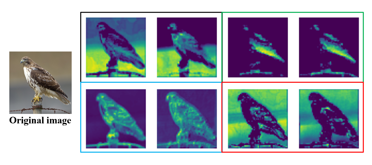
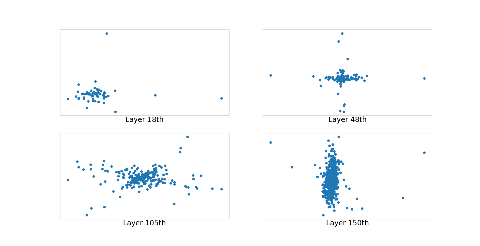
“More-similar-less-important” is another viewpoint to identify pruned filters regardless of their norm. As shown in Fig. 1(a), there are many feature maps pairs of convolutional layers that contain similar semantic information. Such observation has also been pointed out by GhostNet [5], indicating the redundancy is very prevalent on the feature map level, which reveals the similarity of corresponding filters. For further investigation, filters from different depth of the network after decomposition by PCA are visualized in Fig. 1(b), which shows the phenomenon of closing to each other and forming clusters. Although methods like FPGM [11] and FPKM [26] prune the network from this perspective, setting redundant filter to zero will undoubtedly bring information loss, since similar filters does not mean zero contribution.
To address the problems of distribution sensitive and semantic information loss that mentioned above, in this paper, we propose a novel model pruning method based on clustering. Instead of zeroing out unimportant filters, we intend to set them as value of cluster centroids to preserve their ability of extracting features while training. After convergence, we obtain a network whose filters are divided into several clusters and exactly identical within each cluster. Due to the linear and combinational properties of convolutional layer, we can then discard all but to keep one filter of each clusters of current layer and add up the parameters along the corresponding channels of the next layer. Pruning such way will cause almost zero performance loss, thus allowing to retrain for a very limited epochs to overcome the effect caused by batch normalization, which avoids the time-consuming fine-tuning process in previous works.
To summarize, our main contributions are three-fold as follows:
-
•
We empirically demonstrate the redundancy of filters through similarity of feature maps and propose the Asymptotic Soft Cluster Pruning (ASCP) to generate identical filters in a soft manner. Multiple guidelines of clustering are given through analysis and can theoretically well protect feature extraction ability of filters.
-
•
To prevent from strong regularization, we adopt different strategies of pruning rate to prune in an asymptotic way. After convergence, the channel-wise addition operation is introduced to remove identical filters without information loss, since the compact network is equivalent to the unpruned one regardless of batch normalization, which suggest our method can omit the time-consuming fine-tuning step.
-
•
Extensive experiments on CIFAR-10 and ImageNet datasets demonstrate the effectiveness and efficiency of the proposed ASCP compared with other state-of-the-art methods.
2 Related Work
In this section, we will give a comprehensive overview of different pruning methods, which can be roughly divided into three aspects, pruning structure, pruning criteria and pruning manner.

Pruning Structure. Early works of network pruning concentrate on fine-grained granularities: weight-level [15], vector-level [36] and kernel level [16]. For the architecture consistency, this type of non-structured methods can only zeroize the unnecessary parameters rather than pruned. The need of saving special coordinate for every weight makes it difficult to satisfy in nowadays trillion-level model. During inference, although the model sizes and number of multiply-accumulate operations are dramatically decreased, the irregular structure of dense matrices requires additional computations and special hardware designs for acceleration. In line with our work, a few methods have been recently proposed for filter-level pruning (i.e., structured pruning), which can reduce both network size and inference speed and are well supported by various off-the-shelf deep learning libraries. By directly deleting redundant filters in current layer, the corresponding kernels in next layer should also be pruned to keep the consistency of architecture.
Pruning Criteria. Selecting a proper criterion to identify filters which need to be pruned is a major point of network pruning. [16] prunes filters with small -norm in each layer, while [6] [21] are based on -norm. [29] uses the Taylor series to estimate the loss change after each filter’s removal and prune the filters that cause minimal training loss change. Network slimming [25] applies LASSO on the scaling factors of BN, by setting the BN scaling factor to zero, channel-wise pruning is enabled. FPGM [11] prunes filters nearest to the geometric median of each layer using Euclidian distance, refraining from the limits of norm-based criterion. [13] indicates activation may also be an indicator, and it introduces Average Percentage Of Zeros (APoZ) to judge if one output activation map is contributing to the result.
Pruning Manner. The traditional hard filter pruning pipeline will reduce the model capacity of the original models, thus facing the problem of unrecoverable performance loss after incorrect pruning. Besides, the overreliance on pre-trained models and huge time cost of fine-tuning make it unsuitable to deploy in real world scenarios. To overcome that, SFP [10] zeroizes pruned filters with a binary mask and updates filters in a soft manner to maintain the capacity of the network. Based on SFP, ASFP [9] gradually increases the pruning rate to alleviate the accuracy drop caused by pruning and stabilize the whole pruning process. STP [31] uses first-order Taylor series to measure the importance of filters while SRFP [2] removes filters smoothly by gradually decaying to zero, so that it can better preserve the trained information. [1] analysis the characteristic of hard manner and soft manner, and propose GHFP to smoothly switch from soft to hard to achieve a balance between performance and convergence speed.
3 Methodology
3.1 Formulation
In this section, we formally introduce the symbol and notation. The deep CNN network can be parameterized by , where , and is the total number of convolutional layers in a network, and represent the height and width of a kernel. and denote the number of output channels and input channels for the -th convolution layer, respectively. The output feature map is calculated by the convolution operation of input feature map and , shown as below:
| (1) |
and denote the -th output channel of output feature maps and the -th filter of the -th layer, respectively. Assume that the pruning rate of -th layer is , then the number of filters after pruning will reduce from to . Accordingly, the size of the pruned output tensor would be . Given a dataset and a desired sparsity level (i.e., the number of remaining filters), hard filter pruning can be formulated as:
| (2) | ||||
where is the loss function (e.g., cross-entropy loss), is the filter set of the pruned network. Typically, hard filter pruning prunes the model layer by layer and fine-tune iteratively to complement the degradation of the performance. However, once filters are pruned, they will not be updated again which may cause capacity reduction. To alleviate that, soft filter pruning (SFP) and its variants prune filters by simply zeroizing them, which can be represented by
| (3) |
where is a Boolean matrix with the same shape as , indicates whether the filter is pruned or not. denotes the Hadamard product. Specifically, if is pruned, otherwise we set .
3.2 Asymptotic Soft Cluster Pruning
Base on the observation that filters are naturally united in each layer, our ASCP intend to manually introduce similar filters to generate redundancy. As depicted in Fig. 2, our pipeline is carried out iteratively till convergence, and then prunes the network with channel addition operation.
Filter Clustering: We first reshape 4D tensor into a 2D matrix of size . Therefore, each column of this 2D matrix stands for the filter of the weight tensor. Then we can regard them as coordinates in high dimensional space and conduct clustering as:
| (4) |
where is the amount of clusters of -th layer, is the cluster centroid which is assigned to. The optimization can be solved by [28] or other clustering algorithms. After clustering, filters in the -th layer can be divided into clusters, where their norm are relatively close and may have a certain linear relationship [11]. Filters within each cluster can generate similar feature maps of the next layer, therefore, the clusters with more filters can be identified as more redundant.
Setting the hyper-parameter properly is quite critical, since it determines the performance of network after pruning. Next, we propose three guidelines for effectively setting.
Guideline 1: Silhouette Coefficient. With the common used Silhouette Coefficient, we can set by solving the following optimization:
| (5) | ||||
where denotes the average intra-cluster distance (i.e., the average distance between within a cluster), and is the average inter-cluster distance, which means the average distance between and filters within all other clusters.
Guideline 2: Constant over layers. Although Silhouette Coefficient can be precise, such guideline can be quite time-consuming when is large. Besides, if the layer extracts a variety of features, the number of clusters can be massive. This will do harm to the total pruning rate since we need to keep one filter of each cluster, which will be illustrated later in our channel addition operation. In practice, we find that setting to a constant across all layers could perform relatively well for shallow and plain networks (e.g., VGGNet).
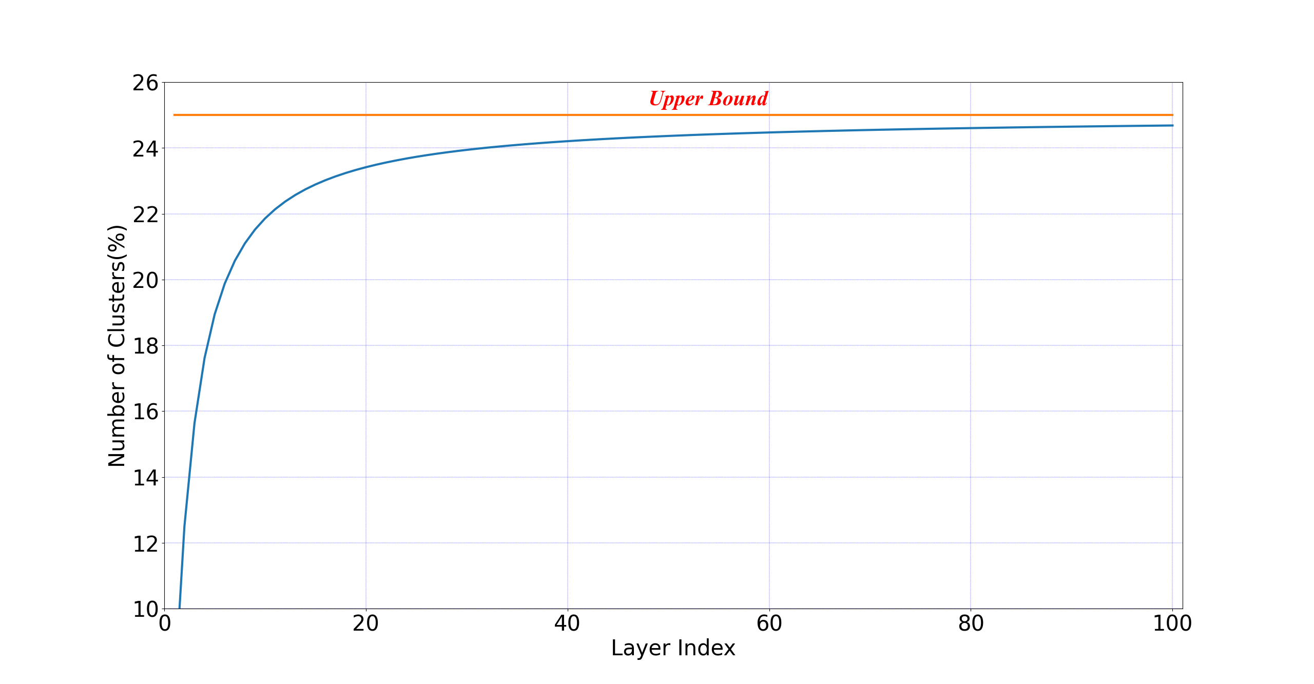
Guideline 3: Adaptive coefficient. However, for a deep and complex structure (e.g. ResNet-50), the above two guidelines can be less effective. As the forward propagation goes, the deeper layers suppose to have more channels to extract various features, which logically should be assigned more clusters. We scale the pruning rate to the worse case and restrict it to satisfy the realistic pruning rate as in Eq. 6, which factually treats as the lower pruning bound. In our experiment, since the pruning rate is same across layers, we can simply scale the arctangent function to modify its upper bound, as shown in Fig. 3(a).
| (6) |
Filter Selection: We adopt the Euclidean distance to evaluate the similarity of filters as Eq. 7. In general, those filters close to assigned cluster centroids would have more redundancy. Based on this understanding, we can find the “most similar” filters and set their values to centroids which they belong to.
| (7) | |||
To avoid severe information loss, we limit to gradually increase from the initial value towards the goal pruning rate . The definition of is list as follows:
| (8) |
where represents the initial pruning rate for the -th layer. To stabilize the pruning process, we consider two kinds of strategies, which are linear increase and exponential increase respectively.
The linear increase strategy can be written as:
| (9) |
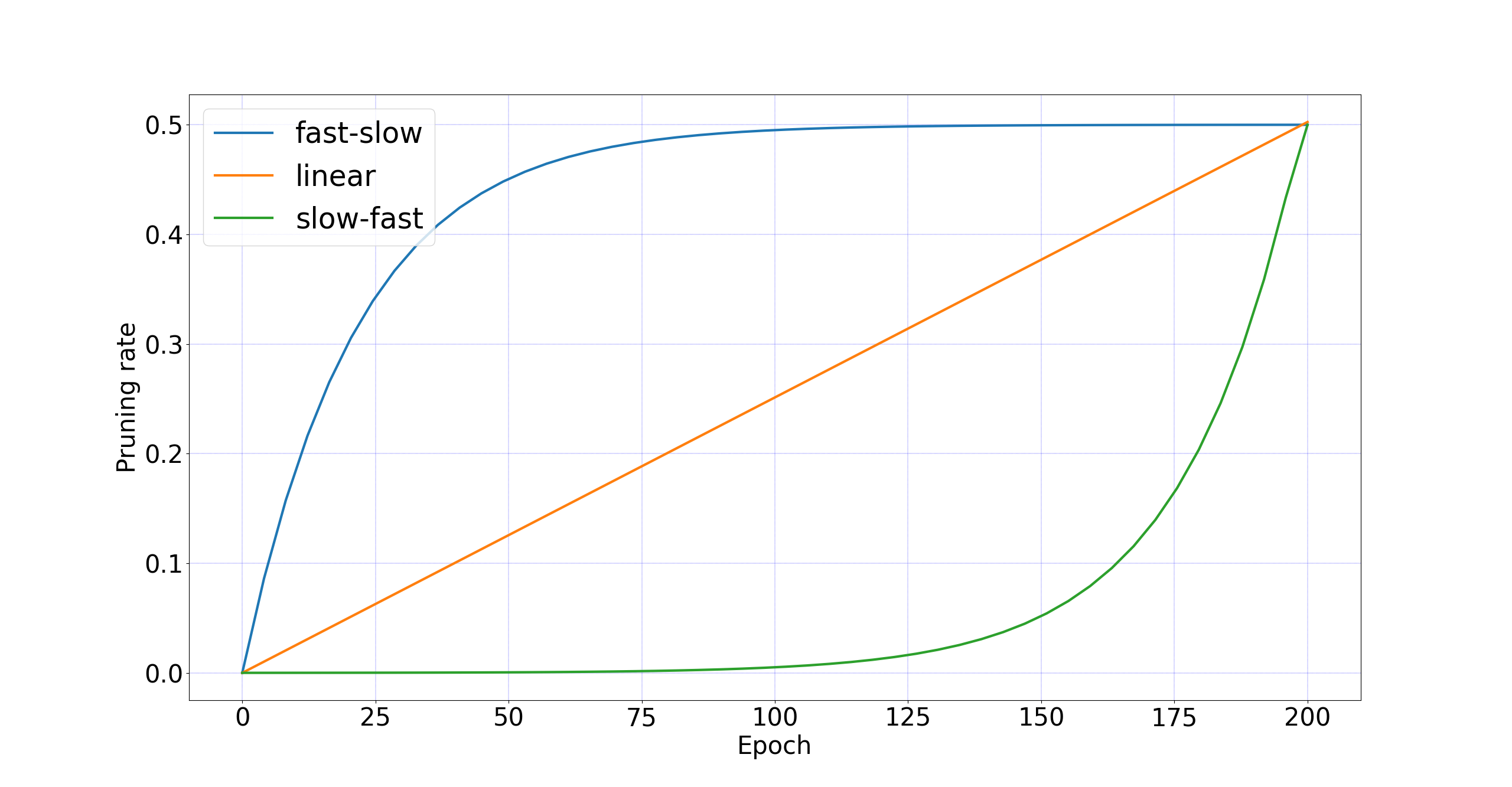
where is the number of total training epochs. Starting from zero, the pruning rate will linearly increase until it reach the goal pruning rate, as illustrated in Fig. 3(b). Similarly, the exponential increase strategy can be given by:
| (10) |
where and are two hyper-parameters to control the growth speed of the pruning rate. For different setting of hyper-parameters, the trend of pruning rate can be fast to slow, or vice versa, as shown in Fig. 3.
Filter Recovery: Filters can be wrongly reconstructed since the cluster centroids are changing along the whole pruning process. Thus after the selection step, we retrain the network for some epochs so that it can recover from the wrong assignment. Furthermore, our method allows the model to keep the same capacity, which ensures the high performance of the model. As the pruning step is integrated into the normal training schema, the model can be trained and pruned synchronously.
Channel Addition: Before convergence, ASCP iterates over the clustering, selection and recovery procedures. When the model converges, it contains lots of identical filters as redundancy, where we can apply channel addition operation to obtain a compact model. As shown in Fig. 2, suppose filters and are identical, we can safely prune one of them by adding corresponding channels of the filters in the next layer, which can be represented by:
| (11) |
where denotes the input feature map of +1-th layer after pruning . and represent the -th and -th channel of , respectively. is the complementary set of . Although the parameters of batch normalization are ignored, we can simply eliminate this effect by fine-tuning for a few epochs. Therefore, there will be no influence to remove these filters as well as the corresponding feature maps. The details of our ASCP are illustrated in Algorithm 1.
| Depth | Method | Baseline(%) | Pruned Accu.(%) | Accu. Drop(%) | Pruned FLOPs(%) |
|---|---|---|---|---|---|
| 20 | SFP [10] | 92.20 | 91.20 | 1.00 | 29.3 |
| ASFP [9] | 92.89 | 91.62 | 1.27 | 29.3 | |
| SRFP [2] | 92.32 | 91.47 | 0.85 | 29.3 | |
| GHFP [1] | 92.89 | 92.14 | 0.75 | 29.3 | |
| Ours | 92.17 | 91.73 | 0.44 | 40.8 | |
| 56 | SFP [10] | 93.59 | 92.26 | 1.33 | 52.6 |
| ASFP [9] | 93.59 | 93.12 | 0.47 | 52.6 | |
| SRFP [2] | 93.66 | 92.67 | 0.99 | 52.6 | |
| FPGM [11] | 93.59 | 92.93 | 0.66 | 52.6 | |
| GHFP [1] | 94.85 | 93.84 | 1.01 | 52.6 | |
| Ours | 93.59 | 92.98 | 0.61 | 60.8 | |
| 110 | SFP [10] | 93.68 | 92.90 | 0.78 | 52.3 |
| ASFP [9] | 94.33 | 93.52 | 0.81 | 52.3 | |
| ASFRP [2] | 94.33 | 93.66 | 0.67 | 52.3 | |
| GHFP [1] | 94.76 | 94.38 | 0.38 | 52.3 | |
| Ours | 94.17 | 93.81 | 0.36 | 61.5 |
4 Experiment
4.1 Experimental Settings
Datasets. We conduct experiments on two publicly available datasets CIFAR-10 [14] and ImageNet [32] to show the efficiency of our method. CIFAR-10 dataset contains 60000 32*32 images with 10 classes, 50000 images for training while the remaining for testing. ImageNet is a large-scale dataset which contains 1.28 million 224*224 training images and 50k validation images drawn from 1000 categories. For both datasets, we first preprocess the data by subtracting the mean and dividing the standard-deviation, then adopt the same data augmentation scheme as [27] [12].
Network Architecture. We study the performance on various mainstream CNN models, including VGGNet [33] with a plain structure and ResNet series [8] with residual blocks. For CIFAR-10 dataset, we test our ASCP on VGGNet, ResNet-20, 56 and 110, while on ImageNet, we test it on ResNet-18, 34 and 50. Since ResNet is less redundant than VGGNet, we will focus more on it.
Configurations. The models are trained from scratch using SGD with a weight decay of 0.0005 and Nesterov momentum of 0.9 [34]. For CIFAR-10, we train the model with a batchsize of 128 for 200 epochs and use an initial learning rate as 0.1, while on ImageNet, the number of epochs, batchsize and the initial learning rate are set to 100, 256 and 0.1, respectively. The learning rate is divided by 5 at epoch 60, 120, 160 on CIFAR-10, and is divided by 10 every 30 epochs on ImageNet. We prune all the convolutional layers of VGGNet for it has a plain structure. While for ResNet, due to the existence of shortcut, we prune all the convolutional layers except for the last one of every residual block for simplification. The pruning operation is conducted after every training epoch with the same pruning rate across all selected layers. We compare our results with other state-of-the-art filter pruning methods, e.g., SFP[10], ASFP[9], SRFP/ASFRP[2], FPGM[11], GHFP[1], AutoPrune[37], VCNNP[40], GAL[22], GS[18], Hrank[19], and all the results are obtained from the original papers. We conduct each experiment for 3 times and report the mean value for comparison.
| Method | Baseline(%) | Pruned Accu.(%) | Accu. Drop(%) | Pruned FLOPs(%) |
|---|---|---|---|---|
| AutoPrune [37] | 92.40 | 91.50 | 0.9 | 23.0 |
| Ours(0.4) | 93.87 | 93.92 | -0.05 | 37.1 |
| VCNNP [40] | 93.25 | 93.18 | 0.07 | 39.1 |
| GAL [22] | 93.96 | 90.73 | 3.23 | 45.2 |
| GS [18] | 94.02 | 93.59 | 0.43 | 60.9 |
| Ours(0.6) | 93.87 | 93.51 | 0.36 | 61.9 |
| Hrank [19] | 93.96 | 92.34 | 1.62 | 65.3 |
| Ours(0.7) | 93.87 | 92.72 | 1.15 | 72.2 |
4.2 Pruning Results on CIFAR-10
| Depth | Method |
|
|
|
|
|
||||||||||
|---|---|---|---|---|---|---|---|---|---|---|---|---|---|---|---|---|
| 18 | SFP [10] | 70.28/67.10 | 89.63/87.78 | 3.18 | 1.85 | 41.8 | ||||||||||
| ASFP [9] | 70.23/68.02 | 89.51/88.19 | 2.21 | 1.32 | 41.8 | |||||||||||
| ASRFP [2] | 70.23/67.25 | 89.51/87.59 | 2.98 | 1.92 | 41.8 | |||||||||||
| Ours | 69.74/67.76 | 89.18/87.95 | 1.98 | 1.23 | 45.6 | |||||||||||
| 34 | SFP [10] | 73.92/71.83 | 91.62/90.33 | 2.09 | 1.29 | 41.1 | ||||||||||
| ASFP [9] | 73.92/72.53 | 91.62/91.04 | 1.39 | 0.58 | 41.1 | |||||||||||
| ASRFP [2] | 73.92/71.39 | 91.62/90.23 | 2.53 | 1.39 | 41.1 | |||||||||||
| FPGM [11] | 73.92/71.79 | 91.62/90.70 | 2.13 | 0.92 | 41.1 | |||||||||||
| Ours | 73.15/71.96 | 91.15/90.58 | 1.19 | 0.57 | 45.1 | |||||||||||
| 50 | SFP [10] | 76.15/74.61 | 92.87/92.06 | 1.54 | 0.87 | 41.8 | ||||||||||
| ASFP [9] | 76.15/75.53 | 92.87/92.73 | 0.62 | 0.14 | 41.8 | |||||||||||
| SRFP [2] | 76.15/75.98 | 92.87/92.81 | 0.17 | 0.06 | 41.8 | |||||||||||
| Ours | 75.56/75.13 | 92.70/92.55 | 0.43 | 0.15 | 48.5 |
ResNet-20/56/110. We conduct our experiment on ResNet-20, 56, 110 for CIFAR-10 dataset. After pruning the pre-trained model, it is finetuned to recover performance. We summarize the results in Table 1, our ASCP achieves comparable performance on CIFAR-10 compared with other filter pruning methods. For example, ASFP accelerates ResNet-56 by 52.6 with 1.20 accuracy drop while our ASCP can prune 60.8 of total FLOPs with only 0.61 accuracy drop. Notably, when the pruning rate is relatively small, these pruning techniques can not make a big gap with each other. However, as the pruning rate becomes larger, ASCP outperforms with only 0.36 accuracy loss and 61.5 of total FLOPs pruned on ResNet-110. This is because ASCP keeps the similar features instead of forcing them towards zeros as other SFP based methods, which demonstrated our ASCP can well protect feature extraction ability of the pruned model.
VGG-16. Table 2 shows the performance of different pruning techniques on VGG-16. We set the number of clusters to 25 of the total amount of filters in each layer to prune the pre-trained model, and then varies the pruning rate between 0.4/0.6/0.7 for better comparison. Our ASCP provides lower accuracy loss compared to AutoPrune and VCNNP (-0.05 v.s. 0.07, 0.9) with similar FLOPs reduction. Compared with GAL and Hrank, ASCP outperforms each of them in all aspects (45.2 v.s. 61.9 and 65.3 v.s. 72.2 in FLOPs reduction, 0.36 v.s. 3.23 and 1.15 v.s. 1.62 in accuracy loss), which proves its ability to compress and accelerate a neural network with a plain structure.
4.3 Pruning Results on ImageNet
For the ImageNet dataset, we evaluate our ASCP on ResNet-18, 34 and 50. We do not prune the last layer of each residual block and the projection shortcuts for simplification. For ResNet-50, since it has the bottleneck structure which contains three convolutional layers in each block, the actual pruned FLOPs will be larger than ResNet-18 and 34 under same pruning rate. Table 3 shows the performance of our ASCP compared with previous mentioned methods. As a result, our method can achieve better FLOPs reduction and lower accuracy drop, for instance, our ASCP can prune 48.5 FLOPs of ResNet-50 with only 0.43 top-1 and 0.15 top-5 accuracy drop.
4.4 Ablation Study
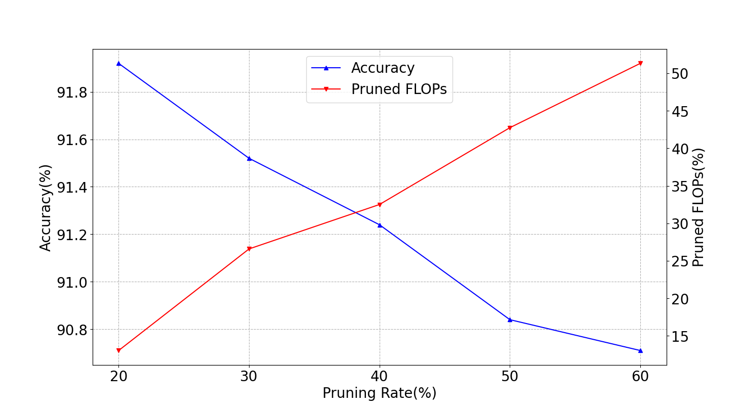
Varying pruning rates. To better shed light on the performance of our ASCP, we present the test accuracy under different pruning rate for ResNet-20 in Fig. 4(a). The network is trained from scratch with the number of clusters is fixed at 25 without fine-tuning. As shown in Fig. 4(a), with the decrease of pruning rate, the test accuracy increases linearly, and the pruned FLOPs decreases gradually as well. When the pruning rate is larger than 50, the accuracy loss compared with baseline is more than 1, which is difficult to recover even after fine-tuning. Thus, for a better trade-off between model complexity and performance, the pruning rate should be chosen carefully.
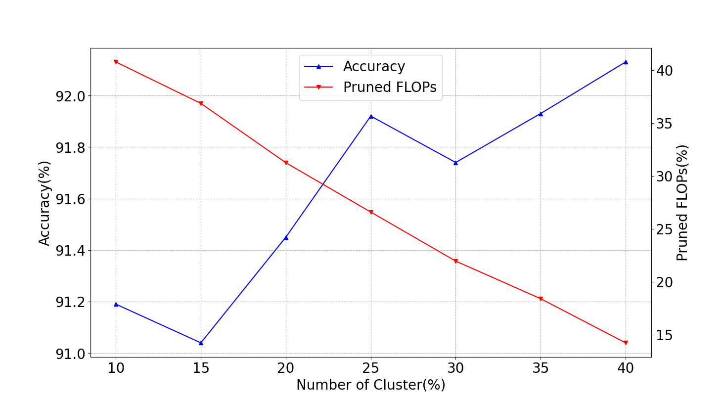
Influence of the number of clusters. In order to explore the influence of , we compare the test accuracy of pruned ResNet-20 with different on CIFAR-10 dataset. As shown in Fig. 4(b), the overall trend of accuracy is that the larger is, the higher test accuracy becomes. However, the pruned FLOPs is also downward and there exists some knee points of accuracy, which suggests that should not be too large and it needs to be well designed to balance the general performance.
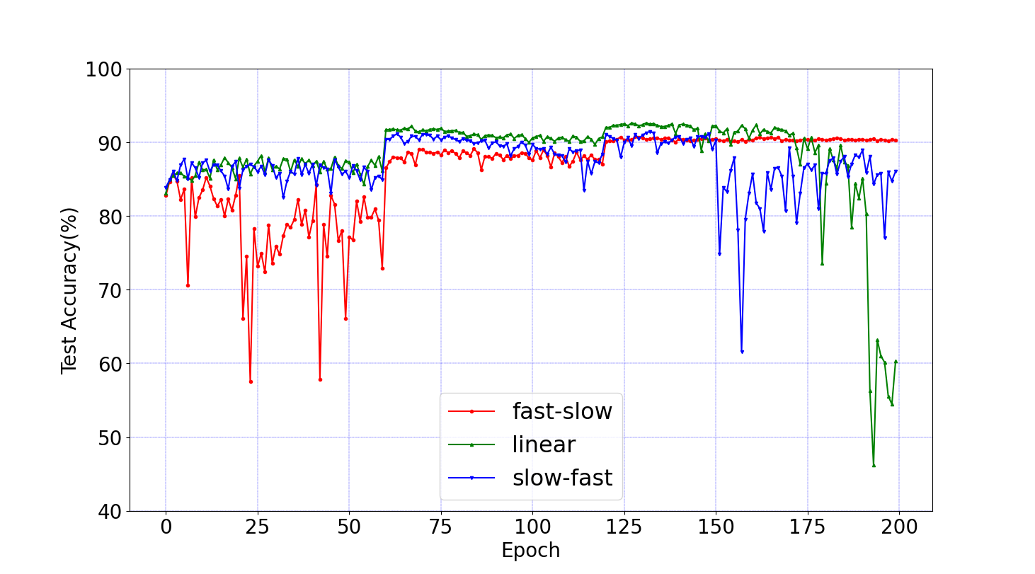
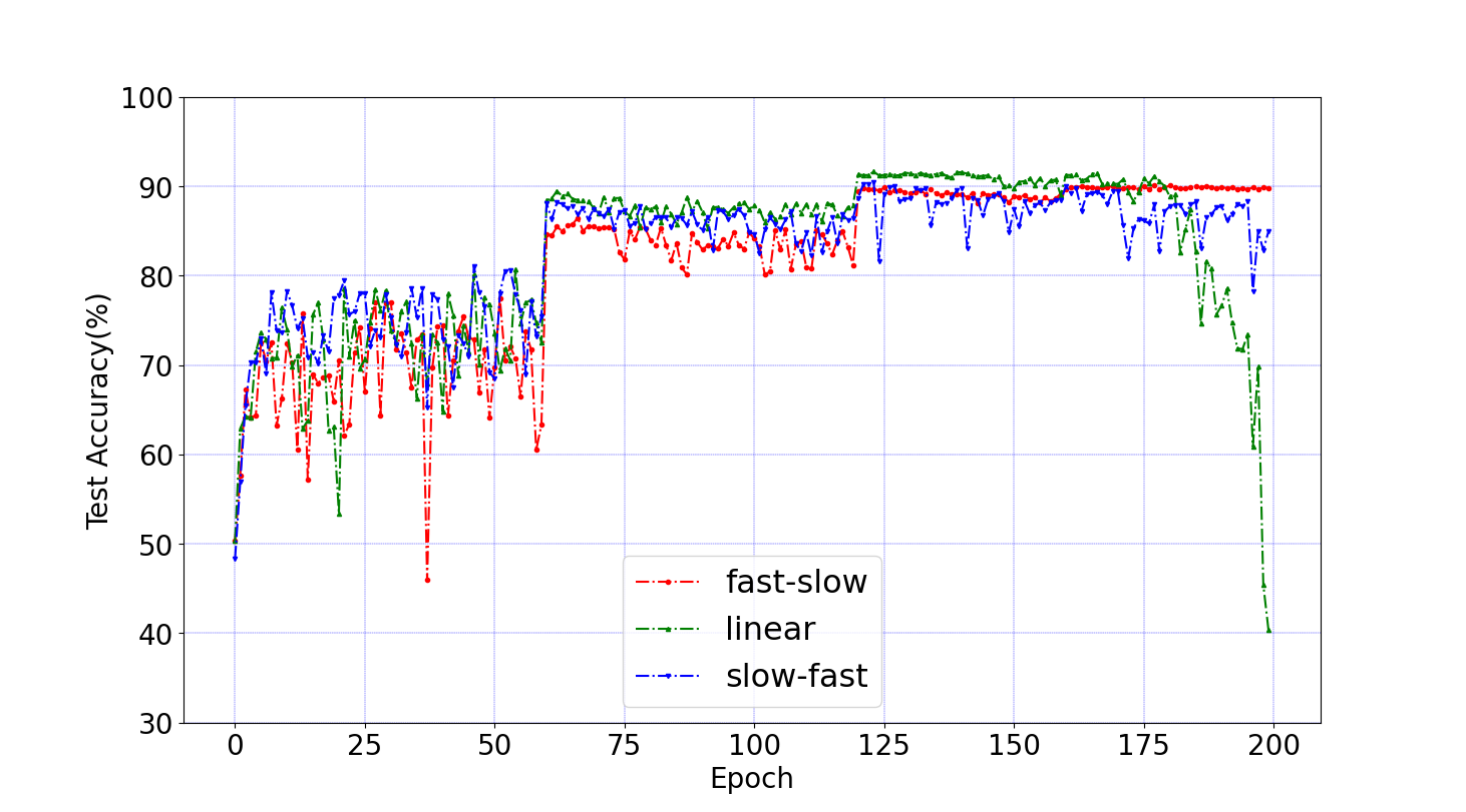
Different pruning strategies. We compare the results of three decay strategies when pruning ResNet-20 on CIFAR-10 with the training epochs increasing. The hyper-parameters and are 0.8 and 25, respectively. As shown in Fig. 5, no matter if it is trained from scratch or not, the fast-slow strategy outperforms others although it causes relatively larger accuracy loss at the initial stage of training process. The linear strategy creates identical filters in a much smoother manner which leads to a disastrous non-convergence issue, so it’s more efficient to use the fast-slow strategy while pruning.
5 Conclusion
To conclude, in this paper, we point out limitations of previous works and propose a novel filter pruning method based on clustering, named ASCP, to accelerate the deep CNNs. Specifically, ASCP considers the similarity between filters as redundancy and removes them in a softer way without information loss. Thanks to these, ASCP allows filters to be pruned more stable as the training procedures run and achieves the state-of-the-art performance in several benchmarks. In the future, we plan to work on how to combine ASCP with other norm-based criteria and more importantly, other acceleration algorithms, e.g., knowledge distillation and matrix decomposition, to push the performance to a higher stage.
6 Acknowledgements
This work was supported in part by the National Key R&D Program of China (No. 2018YFB1201500), the National Natural Science Foundation of China under Grant No. 61771072.
References
- [1] L. Cai, Z. An, C. Yang, and Y. Xu. Soft and hard filter pruning via dimension reduction. In 2021 International Joint Conference on Neural Networks (IJCNN), pages 1–8. IEEE, 2021.
- [2] L. Cai, Z. An, C. Yang, and Y. Xu. Softer pruning, incremental regularization. In 2020 25th International Conference on Pattern Recognition (ICPR), pages 224–230. IEEE, 2021.
- [3] Y. Chen. Convolutional neural network for sentence classification. Master’s thesis, University of Waterloo, 2015.
- [4] Y. Guo, A. Yao, and Y. Chen. Dynamic network surgery for efficient dnns. Advances in neural information processing systems, 29, 2016.
- [5] K. Han, Y. Wang, Q. Tian, J. Guo, C. Xu, and C. Xu. Ghostnet: More features from cheap operations. In Proceedings of the IEEE/CVF Conference on Computer Vision and Pattern Recognition, pages 1580–1589, 2020.
- [6] S. Han, H. Mao, and W. J. Dally. Deep compression: Compressing deep neural networks with pruning, trained quantization and huffman coding. arXiv preprint arXiv:1510.00149, 2015.
- [7] S. Han, J. Pool, J. Tran, and W. Dally. Learning both weights and connections for efficient neural network. Advances in neural information processing systems, 28, 2015.
- [8] K. He, X. Zhang, S. Ren, and J. Sun. Deep residual learning for image recognition. In Proceedings of the IEEE conference on computer vision and pattern recognition, pages 770–778, 2016.
- [9] Y. He, X. Dong, G. Kang, Y. Fu, C. Yan, and Y. Yang. Asymptotic soft filter pruning for deep convolutional neural networks. IEEE transactions on cybernetics, 50(8):3594–3604, 2019.
- [10] Y. He, G. Kang, X. Dong, Y. Fu, and Y. Yang. Soft filter pruning for accelerating deep convolutional neural networks. arXiv preprint arXiv:1808.06866, 2018.
- [11] Y. He, P. Liu, Z. Wang, Z. Hu, and Y. Yang. Filter pruning via geometric median for deep convolutional neural networks acceleration. In Proceedings of the IEEE/CVF Conference on Computer Vision and Pattern Recognition, pages 4340–4349, 2019.
- [12] Y. He, X. Zhang, and J. Sun. Channel pruning for accelerating very deep neural networks. In Proceedings of the IEEE international conference on computer vision, pages 1389–1397, 2017.
- [13] H. Hu, R. Peng, Y.-W. Tai, and C.-K. Tang. Network trimming: A data-driven neuron pruning approach towards efficient deep architectures. arXiv preprint arXiv:1607.03250, 2016.
- [14] A. Krizhevsky, G. Hinton, et al. Learning multiple layers of features from tiny images. 2009.
- [15] Y. LeCun, J. Denker, and S. Solla. Optimal brain damage. Advances in neural information processing systems, 2, 1989.
- [16] H. Li, A. Kadav, I. Durdanovic, H. Samet, and H. P. Graf. Pruning filters for efficient convnets. arXiv preprint arXiv:1608.08710, 2016.
- [17] Y. Li, S. Gu, C. Mayer, L. V. Gool, and R. Timofte. Group sparsity: The hinge between filter pruning and decomposition for network compression. In Proceedings of the IEEE/CVF conference on computer vision and pattern recognition, pages 8018–8027, 2020.
- [18] Y. Li, S. Gu, C. Mayer, L. V. Gool, and R. Timofte. Group sparsity: The hinge between filter pruning and decomposition for network compression. In Proceedings of the IEEE/CVF conference on computer vision and pattern recognition, pages 8018–8027, 2020.
- [19] M. Lin, R. Ji, Y. Wang, Y. Zhang, B. Zhang, Y. Tian, and L. Shao. Hrank: Filter pruning using high-rank feature map. In Proceedings of the IEEE/CVF conference on computer vision and pattern recognition, pages 1529–1538, 2020.
- [20] S. Lin, R. Ji, Y. Li, C. Deng, and X. Li. Toward compact convnets via structure-sparsity regularized filter pruning. IEEE transactions on neural networks and learning systems, 31(2):574–588, 2019.
- [21] S. Lin, R. Ji, Y. Li, Y. Wu, F. Huang, and B. Zhang. Accelerating convolutional networks via global & dynamic filter pruning. In IJCAI, volume 2, page 8, 2018.
- [22] S. Lin, R. Ji, C. Yan, B. Zhang, L. Cao, Q. Ye, F. Huang, and D. Doermann. Towards optimal structured cnn pruning via generative adversarial learning. In Proceedings of the IEEE/CVF Conference on Computer Vision and Pattern Recognition, pages 2790–2799, 2019.
- [23] T.-Y. Lin, M. Maire, S. Belongie, J. Hays, P. Perona, D. Ramanan, P. Dollár, and C. L. Zitnick. Microsoft coco: Common objects in context. In European conference on computer vision, pages 740–755. Springer, 2014.
- [24] Z. Lin, M. Courbariaux, R. Memisevic, and Y. Bengio. Neural networks with few multiplications. arXiv preprint arXiv:1510.03009, 2015.
- [25] Z. Liu, J. Li, Z. Shen, G. Huang, S. Yan, and C. Zhang. Learning efficient convolutional networks through network slimming. In Proceedings of the IEEE international conference on computer vision, pages 2736–2744, 2017.
- [26] Z. Liu, P. Wang, and Z. Li. More-similar-less-important: Filter pruning via kmeans clustering. In 2021 IEEE International Conference on Multimedia and Expo (ICME), pages 1–6. IEEE, 2021.
- [27] J.-H. Luo, J. Wu, and W. Lin. Thinet: A filter level pruning method for deep neural network compression. In Proceedings of the IEEE international conference on computer vision, pages 5058–5066, 2017.
- [28] J. MacQueen et al. Some methods for classification and analysis of multivariate observations. In Proceedings of the fifth Berkeley symposium on mathematical statistics and probability, volume 1, pages 281–297. Oakland, CA, USA, 1967.
- [29] P. Molchanov, S. Tyree, T. Karras, T. Aila, and J. Kautz. Pruning convolutional neural networks for resource efficient inference. arXiv preprint arXiv:1611.06440, 2016.
- [30] S. Ren, K. He, R. Girshick, and J. Sun. Faster r-cnn: Towards real-time object detection with region proposal networks. Advances in neural information processing systems, 28, 2015.
- [31] J. Rong, X. Yu, M. Zhang, and L. Ou. Soft taylor pruning for accelerating deep convolutional neural networks. In IECON 2020 The 46th Annual Conference of the IEEE Industrial Electronics Society, pages 5343–5349. IEEE, 2020.
- [32] O. Russakovsky, J. Deng, H. Su, J. Krause, S. Satheesh, S. Ma, Z. Huang, A. Karpathy, A. Khosla, M. Bernstein, et al. Imagenet large scale visual recognition challenge. International journal of computer vision, 115(3):211–252, 2015.
- [33] K. Simonyan and A. Zisserman. Very deep convolutional networks for large-scale image recognition. arXiv preprint arXiv:1409.1556, 2014.
- [34] I. Sutskever, J. Martens, G. Dahl, and G. Hinton. On the importance of initialization and momentum in deep learning. In International conference on machine learning, pages 1139–1147. PMLR, 2013.
- [35] Z. Wang, F. Li, G. Shi, X. Xie, and F. Wang. Network pruning using sparse learning and genetic algorithm. Neurocomputing, 404:247–256, 2020.
- [36] W. Wen, C. Wu, Y. Wang, Y. Chen, and H. Li. Learning structured sparsity in deep neural networks. Advances in neural information processing systems, 29, 2016.
- [37] X. Xiao, Z. Wang, and S. Rajasekaran. Autoprune: Automatic network pruning by regularizing auxiliary parameters. Advances in neural information processing systems, 32, 2019.
- [38] F. Yu, C. Han, P. Wang, R. Huang, X. Huang, and L. Cui. Hfp: Hardware-aware filter pruning for deep convolutional neural networks acceleration. In 2020 25th International Conference on Pattern Recognition (ICPR), pages 255–262. IEEE, 2021.
- [39] S. Zagoruyko and N. Komodakis. Paying more attention to attention: Improving the performance of convolutional neural networks via attention transfer. arXiv preprint arXiv:1612.03928, 2016.
- [40] C. Zhao, B. Ni, J. Zhang, Q. Zhao, W. Zhang, and Q. Tian. Variational convolutional neural network pruning. In Proceedings of the IEEE/CVF Conference on Computer Vision and Pattern Recognition, pages 2780–2789, 2019.