Modeling racial/ethnic differences in COVID-19 incidence with covariates subject to non-random missingness

Abstract

Characterizing the cumulative burden of COVID-19 by race/ethnicity is of the utmost importance for public health researchers and policy makers in order to design effective mitigation measures. This analysis is hampered, however, by surveillance case data with substantial missingness in race and ethnicity covariates. Worse yet, this missingness likely depends on the values of these missing covariates, i.e. they are not missing at random (NMAR). We propose a Bayesian parametric model that leverages joint information on spatial variation in the disease and covariate missingness processes and can accommodate both MAR and NMAR missingness. We show that the model is locally identifiable when the spatial distribution of the population covariates is known and observed cases can be associated with a spatial unit of observation. We also use a simulation study to investigate the model’s finite-sample performance. We compare our model’s performance on NMAR data against complete-case analysis and multiple imputation (MI), both of which are commonly used by public health researchers when confronted with missing categorical covariates. Finally, we model spatial variation in cumulative COVID-19 incidence in Wayne County, Michigan using data from the Michigan Department and Health and Human Services. The analysis suggests that population relative risk estimates by race during the early part of the COVID-19 pandemic in Michigan were understated for non-white residents compared to white residents when cases missing race were dropped or had these values imputed using MI.

, , and

1 Introduction

Complete and detailed surveillance data are critical sources of information for decision-making and communication in public health emergencies like the COVID-19 pandemic. Under ideal conditions, these data can provide an indication of emerging trends, e.g. growth in socioeconomic inequity in infection and disease risk, which can be used to craft policies and target resources. For example, after surveillance data pointed to wide racial/ethnic disparities in incidence and mortality in the COVID-19 pandemic in the United States (Millett et al., 2020; Zelner et al., 2021), policies intended to narrow the gap were put in place Office of Michigan Governor (2020); Governor Whitmer Executive Order (2020). However, without adequate information on the distribution of infection within and between different socioeconomic and race/ethnic groups, the impact of such policy measures is difficult to evaluate.

Missing covariates have long been a challenge associated with administrative datasets, such as public health surveillance data, and the scale and importance of this problem has only grown during the COVID-19 pandemic (Labgold et al., 2021; Millett et al., 2020). Covariate missingness in surveillance data may result from a variety of mechanisms, ranging from non-response on an intake form, refusal to participate in tracing interviews, or data-entry errors after these data are collected. Often this missingness is implicitly or explicitly assumed to occur at random, i.e. not as a function of the disease process or the attributes of individual cases. But if the process causing case data to be missing important categorical variables, e.g. age, race, sex, or neighborhood, is dependent on the disease process, excluding cases that are missing these covariates may result in estimates that are overconfident and biased. Furthermore, the direction of this bias is not easy to characterize, and may result in over- or under-estimates of group-level differences in risk as epidemic conditions shift.

In emergency situations, such as a surging pandemic, it is easy to see how the disease process itself may induce non-random missingness of covariates. For example, during a period of rapidly increasing caseloads, such as the Delta and Omicron surges of the COVID-19 pandemic, the overwhelming number of cases is likely to limit the ability of case investigators to collect data that are as detailed as those collected during lower-incidence periods. These differences may also be more pronounced when comparing wealthier and poorer jurisdictions with differential resources for case-finding and intervention. When these differential risks and resources are concentrated in communities with large proportions of non-White residents, the likelihood that the missingness of key demographic information, including race/ethnicity, will depend on the race of respondents is high. The intensity of this missingness is also likely to vary in space, reflecting numerous factors including differences in epidemic conditions as well as varying data quality across public health jurisdictions.

Both of these characteristics point to a nonignorable missing data problem, as presented in Rubin (1976). Both issues make quantifying the relative risk of infection among population strata during the COVID-19 pandemic potentially error-prone: high proportions of cases are missing demographic data, with missingness that is likely differential across population strata. It is in this scenario that omitting cases with missing demographic data may yield biased estimates of relative risk. Tools that assume ignorability, like multiple imputation methods typically do (Audigier et al., 2018), cannot correct for missingness that depends on the value of the covariate, and will thus incur bias as well. This problem is not exclusive to the challenge of characterizing sociodemographic disparities in infection risk: incomplete reporting of vaccination status may lead to difficulty in estimating risks of breakthrough COVID-19 infections among vaccinated people, and missing information on comorbid conditions increasing the risk of death may complicate efforts at estimating risks of death associated with infection.

In order to employ statistical methods that appropriately account for missingness, such as those presented in Little and Rubin (2002), one must make the modeling assumptions explicit in a joint probability model for the outcome variable, the covariate subject to missingness, and the missingness process for that covariate. When the missingness process is nonignorable, two broad classes of models can be used to encode the assumptions about the joint distribution: selection models and pattern mixture models (Little and Rubin, 2002). There is much literature on the theoretical and practical applications of both classes of models: Diggle and Kenward (1994); Clark and Houle (2014); Roy and Daniels (2008). For a review of selection and pattern mixture models see Little (2008) and Little (1995).

We develop a novel model that accounts for nonignorable missingness of demographic covariates for which there is known population data, as in Zangeneh (2012), but we take a selection model approach instead of a pattern mixture model approach. Our probabilistic model is similar to that of Stasny (1991), wherein Stasny develops a selection model for nonignorable missingness in binary survey data, though we incorporate ideas from Zangeneh (2012) in using known census demographic data. Our approach is to develop a model that allows for simultaneous modeling of the disease and missingness processes, and that incorporates information on spatial clustering of risk in addition to sociodemographic risk factors. Given the ubiquity of missing categorical covariates in public health surveillance data and the generality of our model, there are many potential applications of this class of models.

1.1 Alternative approaches

Because missing data can lead to ineffective and potentially life-threatening decision-making in public health and medicine, analysis of epidemiological data subject to missingness is an area of active research. This work, however, is often focused on accounting for data missing-at-random or on imputing values of continuous covariates. Recent work focusing on accounting for missing covariates when modeling disease data in space and time like Holland, Jones and Benschop (2015); Gómez-Rubio, Cameletti and Blangiardo (2019); Baker, White and Mengersen (2014) suffer from several limitations. Gómez-Rubio, Cameletti and Blangiardo (2019) presents a framework for joint modeling of the disease process and missingness process, which can incorporate NMAR missingness, but only for continuous covariates. When missing covariates are discrete, Gómez-Rubio, Cameletti and Blangiardo resort to multiple imputation, which compromises statistical efficiency gained from joint modeling, increases the computational burden, and assumes MAR missingness. Holland, Jones and Benschop (2015) does include a model for discrete missing covariates with an outcome model, but the missing data mechanism is assumed to be MAR. In other work, Baker, White and Mengersen (2014) developed a cross-validation approach to missing data imputation, but assume MAR missingness. Recent work in applications for missing data continue to assume MAR (Aguayo et al., 2020; Labgold et al., 2021). As we argue above, assuming missingness is MAR can bias inferences; Perkins et al. (2018); Sidi and Harel (2018); Stavseth, Clausen and Røislien (2019) explore how mistaken assumptions in the missing data model impact inferences. When missing data are inherently social in nature, MAR assumptions become even more tenuous than they might be in other settings. In the context of the COVID-19 pandemic, missingness of race/ethnicity data reflects a host of factors, including socioeconomic biases in the quality and thoroughness of public health data systems, which effectively guarantee correlation between the race/ethnicity of the respondent and their likelihood of missing these data. This paucity of recent work in spatial epidemiology employing an NMAR missingness model for discrete missing covariates, and the urgency of improving the quality of inferences from public health surveillance data provided the primary motivation for the development of our model.

The most germane work is Labgold et al. (2021), which applies Bayesian Improved Surname Geocoding (BISG) to the estimation of race/ethnicity disparities in COVID-19 incidence using data from Fulton County, Georgia. BISG was originally developed in Elliott et al. (2009) for understanding disparities in health outcomes when race data are not available. The approach is an extension of a geocoding model for race, which generates a categorical distribution over race using the location of the unit of analysis (in Labgold et al. the unit of analysis is a case-patient notified of a positive SARS-CoV-2 test). BISG adds surname information to this categorical distribution, with the intention of more accurately imputing race. The weakness of this approach is that the imputation is not informed by the outcome model or vice versa. In the infectious disease context, the information that many cases for which one observes race or ethnicity should inform the categorical distribution for cases missing race information. Labgold et al. addresses this limitation by further modeling the misclassification rate for BISG by comparing BISG’s imputed race to that of race for case-patients not missing race. The procedure, however, does not correspond to a probabilistic model, which makes it challenging to validate its implicit assumptions. Furthermore, BISG assumes that the missingness process is missing-at-random, which may not be a good assumption in the context of missing race data. Zhang et al. (2022) also accounts for missing race data in COVID-19 cases via multiple imputation, again assuming MAR missingness.

Despite the wide-ranging literature on analyzing case with missing covariates, a common practice among academic and applied researchers is to omit observations with missing covariates, performing what is known as “complete case analysis”, when confronted with missing data (Eekhout et al., 2012). For example, complete case analysis has been used in studies of racial/ethnic disparities of COVID-19 burden when race/ethnicity data are missing (Millett et al., 2020; Zelner et al., 2021) despite the authors’ acknowledgement of the risks inherent in dropping incomplete cases. This is an indication of the pervasiveness of the practice, in part due to the ease of performing complete case analysis in most statistical packages (e.g. the ubiquitous na.rm=TRUE argument in the R language) and in part due to the lack of methods available to researchers for nonignorable missingness. That complete case analysis is widely employed should galvanize methodologists to develop techniques that are more finely attuned to infectious disease epidemiology.

1.2 Considerations when imputing missing demographic information

Imputing missing demographic data presents multiple challenges at the intersection of ethics, sociology, and statistics (Kennedy et al., 2020). Kennedy et al. note that, beyond the formidable statistical challenges, dealing with missing data of this nature requires understanding how demographic categories in administrative data have changed over time, the relationship between official categories and categories that individuals use to identify themselves, and the fact that attributes like sex, gender, and race/ethnicity must be understood through an intersectional lens rather than as independent dimensions of identity. Furthermore, the authors note that to the extent that there is an imbalance in how groups are misrepresented in surveys, even imputation with uncertainty confers statistical bias and, ultimately, discrimination. The authors argue that despite these realities and being bound by data availability and antiquated study designs, researchers must take responsibility for the choices they make in handling missing data.

Omitting cases that have missing data may be mistaken as a safe practice when missingness of demographic information is assumed - implicitly or explicitly - to occur at random. However, in real-world public health surveillance data, it is unlikely that such information will be missing at random. Instead, there is a high likelihood that the rate of missingness will be correlated with the burden of disease in a community and the resources local authorities have to address it, which are in turn often reflected in race/ethnic disparities in disease outcomes. As this burden increases and the financial and material tools to find new cases dwindle, it becomes increasingly likely that race/ethnic minority groups will be subject to higher rates of missingness which are positively associated with disease risk. This intuition is reflected in our results, which show that when missingness does not occur completely random, dropping cases can result in biased estimates and overstatement of certainty in these estimates.

Furthermore, even when the data are missing completely at random - the most innocuous scenario - random variation in which cases are missing can amount to statistical bias in finite samples. Kennedy et al. note that this can serve as a form of discrimination if the conclusions from the analysis are used to draw inferences about the population and make decisions. This is particularly problematic when addressing missingness for groups that represent a small share of the observed data or overall population: In this case, dropping even a small number of cases missing data can result in diminished power to make valid inferences about group-specific risks. Because of this, making every effort to account for all sources of information on race/ethnicity, even those that are plausibly missing at random, is an ethical imperative.

Exact probabilistic imputation, like the approach we present below, avoids some, but not all, of the risks of wrongly imputing demographic characteristics associated with deterministic approaches. As Kennedy et al. point out, probabilistic imputation does not guarantee bias-free conclusions, especially if the procedure’s misclassification rates are not equally distributed across demographic subgroups. For example, a model that mistakenly assumes that the missingness process is ignorable risks under-representing groups for which the baseline rate of missingness is higher or for whom missingness is positively correlated with the disease process. A well-designed procedure, with results interpreted with awareness of simplifying assumptions and their potential to induce bias, can facilitate increased relevance of study results for underrepresented groups, while also providing a more appropriate representation of uncertainty in these conclusions.

1.3 Paper roadmap

In this paper, we present a new joint model that allows researchers to account for relationships between variation in the disease outcome measure of interest and the missingness process. This approach makes the flow of information and model assumptions clear, while at the same time affording researchers all the tools that have been developed to interrogate, summarize and present results from a coherent probabilistic model.

In the following sections, we will 1) Describe the justification for our approach and theoretical properties of the model, 2) Conduct a detailed simulation study to investigate the finite-sample performance of the model under several known data-generating processes, and finally, 3) Apply this model to detailed COVID-19 data from southeastern Michigan.

2 Methods

Suppose for each resident, indexed by $n$, in a large population with size $E$, the variable $U_{n}$ is a binary random variable that represents a diagnostic test result (e.g. COVID-19 polymerase chain reaction (PCR) test), $C_{n}$ is a categorical variable with $J$ levels that encodes race/ethnicity information which may be missing for some residents, $R_{n}$ is an indicator variable equal to $1$ if $C_{n}$ is observed and $0$ otherwise, and $S_{n}$ is a categorical variable encoding stratum information, like age or sex information for that resident. In other words, each resident is associated with the vector $(U_{n},C_{n},R_{n},S_{n})$, of which $U_{n}$ and $R_{n}$ are assumed to be random variables, while $C_{n}$ and $S_{n}$ are fixed characteristics of each resident.

Let the variable $Y_{ij}$ be the total cases in the population for which $S_{n}=i$ and $C_{n}=j$, or more explicitly,

$$Y_{ij}=\textstyle\sum_{\{n\,|\,S_{n}=i,C_{n}=j\}}U_{n},$$

and let $E_{ij}$ be the total count of the population in stratum $i$ and race/ethnicity $j$:

$$E_{ij}=\sum_{n=1}^{E}\mathbbm{1}_{S_{n}=i}\mathbbm{1}_{C_{n}=j}.$$

Let the set of test results $U_{n}$ for the population be $\mathcal{U}\in\{0,1\}^{E}$. Define $X_{ij}$ as the number of cases in stratum $i$ for which race/ethnicity $C_{n}$ is observed to be $j$ and $M_{i}$ as the number of cases in stratum $i$ as the number of cases missing race/ethnicity information:

$$X_{ij}\,|\,\mathcal{U}=\textstyle\sum_{\{n\,|\,S_{n}=i,C_{n}=j,U_{n}=1\}}R_{n}\quad\text{and}\quad M_{i}\,|\,\mathcal{U}=\textstyle\sum_{j}\sum_{\{n\,|\,S_{n}=i,C_{n}=j,U_{n}=1\}}(1-R_{n})$$

Let $Y_{ij}$ be conditionally independent Poisson random variables: $Y_{ij}|\mu_{ij}\sim\text{Poisson}(\mu_{ij}).$ where we define incidence as

$$\mu_{ij}/E_{ij},$$

or the per-capita rate of disease. We further assume that race/ethnicity observation indicators $R_{n}$ are conditionally independent Bernoulli distributed random variables with probability observing race/ethnicity information denoted as $p_{ij}$, which depends solely on stratum $i$ and race/ethnicity category $j$. Then

$$X_{ij}|\mathcal{U}\overset{d}{=}X_{ij}|Y_{ij},\implies\quad X_{ij}|Y_{ij},p_{ij}\sim\text{Binomial}(Y_{ij},p_{ij})$$

The distributional assumptions imply that marginalizing over total cases of race/ethnicity $j$ in stratum $i$, $Y_{ij}$, yields conditionally independent Poisson random variables:

$$X_{ij}|p_{ij},\mu_{ij}\sim\text{Poisson}(p_{ij}\mu_{ij})$$

for cases of race/ethnicity $j$ observed with race/ethnicity and missing cases are mutually independent of $X_{ij}$ and conditionally independent Poisson random variables:

$$M_{i}|(p_{i1},\mu_{i1}),\dots,(p_{iJ},\mu_{iJ})\sim\text{Poisson}(\textstyle\sum_{j}(1-p_{ij})\mu_{ij})$$

We show the connection between our model and the missing data modeling paradigm introduced by Rubin (1976) and further developed in Little and Rubin (2002) in appendix A, and also show that the model implies that the missingness can be not missing at random (NMAR) if $p_{ij}$ vary by $j$.

Given that $p_{i1}=p_{i2}=\dots=p_{iJ}$ for all $i$ is a strong constraint, allowing the model to learn the extent to which probability of observing race/ethnicity varies by race/ethnicity (i.e. allowing the model to learn how far missingness deviates from MAR) is the most judicious modeling choice.

2.1 Modeling incidence when missingness is dependent on race/ethnicity

We present a simple example of the model below, in which we assume that race/ethnicity is the only characteristic that predicts both disease incidence and the rate of missingness for individual-level race/ethnicity information. As above, we summarise population counts by age-sex stratum $i$ and race/ethnicity category $j$:

$$E_{ij}=\sum_{n=1}^{E}\mathbbm{1}_{S_{n}=i}\mathbbm{1}_{C_{n}=j}.$$

Let $\mathbf{e}_{i}$ be the vector $(E_{i1},\dots,E_{iJ})^{T}$ with the $j^{\rm th}$-element $E_{ij}$, and let

$$\mathbf{E}\in{}^{I\times J}\,\text{such that }\,\mathbf{E}_{[i,:]}=\mathbf{e}_{i}^{T}.$$

If exposure to the disease is governed solely by race/ethnicity, and infection probability and exposure is constant across age-sex strata $i$, then we may assume that $\mu_{ij}=\lambda_{j}E_{ij}$ and that $p_{ij}=p_{j},\forall i$. The observed data model, letting $\boldsymbol{\lambda}=(\lambda_{1},\dots,\lambda_{J})$ and $\mathbf{p}=(p_{1},\dots,p_{J})$, simplifies to the following:

$$\begin{split}X_{ij}|p_{j},\lambda_{j},E_{ij}&\sim\text{Poisson}(p_{j}\lambda_{j}E_{ij}),\\ M_{i}|\mathbf{p},\boldsymbol{\lambda},\mathbf{e}_{i}&\sim\text{Poisson}(\textstyle\sum_{j}\lambda_{j}(1-p_{j})E_{ij});\end{split}$$ (1)

where we have made the conditioning on parameters and population counts explicit.

2.1.1 Identifiability properties of the model

We can show that model (1) is globally identifiable by appealing to Theorem 4 of Rothenberg (1971). Theorem 2.1 shows that the model parameters $(\mathbf{p},\boldsymbol{\lambda})$ are globally identifiable given the observed data under minimal conditions on the parameters, and an easily verifiable condition on the population count matrix $\mathbf{E}$.

Theorem 2.1.

The observational model (1) is globally identifiable under the following conditions:

1. $\mathbf{E}$ is rank $J$,

2. $\lambda_{j}\in(0,\infty)\forall j\in[1,\dots,J]$,

3. $p_{j}\in(0,1)\forall j\in[1,\dots,J]$.

Proof.

Reparameterize the model from $(\lambda_{j},p_{j})$ to $(v_{j},u_{j})$ where $v_{j}=p_{j}\lambda_{j}$ and $u_{j}=(1-p_{j})\lambda_{j}$. Given conditions (E.b) to (E.c), the mapping is one-to-one and onto. Let $\mathbf{u}$ be the $J$-vector with element $j$ equal to $u_{j}$ and let $\mathbf{v}$ be similarly defined for $v_{j}$. The reparameterized model becomes:

$$X_{ij}|v_{j},E_{ij} \sim\text{Poisson}(v_{j}E_{ij})$$ (2)

$$M_{i}|\mathbf{u},\mathbf{e}_{i} \sim\text{Poisson}(\textstyle\sum_{j}u_{j}E_{ij})$$ (3)

We know that $\hat{v}_{j}=\frac{\sum_{i}X_{ij}}{\sum_{i}E_{ij}}$ is unbiased for $v_{j}$. Let $\mathbf{m}$ be the $I$-vector with element $i$ equal to $M_{i}$. Then

$$\mathbb{E}\left[\mathbf{m}\right]=\mathbf{E}\mathbf{u}$$

By condition (E.a)

$$\left(\mathbf{E}^{T}\mathbf{E}\right)^{-1}\mathbf{E}^{T}\mathbb{E}\left[\mathbf{m}\right]=\mathbf{u}.$$ (4)

Given that we can define unbiased estimators for $\mathbf{v}$ and $\mathbf{u}$ , by Theorem 4 in Rothenberg (1971), the model is globally identifiable in $(v_{j},u_{j})$. Given that our mapping from $(\lambda_{j},p_{j})$ to $(v_{j},u_{j})$ is one-to-one and onto, global identifiability in $(v_{j},u_{j})$ implies global identifiability in $(\lambda_{j},p_{j})$ because we can define an inverse mapping from $(v_{j},u_{j})$ to $(\lambda_{j},p_{j})$. ∎

It can also be seen that the variance-covariance matrix for the estimator for $\hat{\boldsymbol{\lambda}}$ is a sum of two components: the variance of $\hat{\mathbf{v}}$ and the variance-covariance matrix of the unbiased linear estimator for $\mathbf{u}$, $\left(\mathbf{E}^{T}\mathbf{E}\right)^{-1}\mathbf{E}^{T}\mathbf{m}$. This coincides with the Fisher information matrix, as derived in Appendix Section D.1, where we also show that the Fisher information matrix is positive definite under conditions (E.a) to (E.c).

2.1.2 Model intuition

We examine a simple setting in which there are two race/ethnicity groups (or equivalently, $J=2$) subject to missingness. The unbiased estimator, $\hat{u}_{1}$, for $u_{1}=(1-p_{1})\lambda_{1}$ can be expressed in terms of a projection matrix:

$$\mathbf{P}_{2}=\mathbf{e}_{2}(\mathbf{e}_{2}^{T}\mathbf{e}_{2})^{-1}\mathbf{e}_{2}^{T}$$

which is the projection for a vector in ^I to the subspace spanned by $\mathbf{e}_{2}$. Then

$$\hat{u}_{1}=\frac{\mathbf{m}^{T}(\mathbf{I}-\mathbf{P}_{2})\mathbf{e}_{1}}{\mathcal{\|}(\mathbf{I}-\mathbf{P}_{2})\mathbf{e}_{1}\|_{2}^{2}}.$$ (5)

which can be understood as a relative measure of the strength of the covariance between the number of cases with missing race/ethnicity information and population counts for group $1$ after accounting for the variation in population counts attributable to group $2$. The following estimator is unbiased for $\lambda_{1}$:

$$\frac{\sum_{i=1}^{I}X_{i1}}{\sum_{i=1}^{I}E_{i1}}+\hat{u}_{1}.$$ (6)

The first term in eq. 6 is the estimator for $\lambda_{1}p_{1}$ for a Poisson distribution with rate $\lambda_{1}p_{1}$, while the second term is a correction to account for missingness. If the covariance of $\mathbf{m}$ and a residualized $\mathbf{e}_{1}$ (by regressing $\mathbf{e}_{1}$ on $\mathbf{e}_{2}$) is large relative to the variance of the residualized $\mathbf{e}_{1}$ then the correction will be large. If, on the contrary, this quantity is small, the correction factor will be small. The estimator depends on the conditional expectation of the number of cases for each race/ethnicity being proportional to the number of residents in that category, which is a common assumption in modeling count data in epidemiology (Frome, 1983; Frome and Checkoway, 1985; Lash et al., 2021).

2.1.3 Bayesian inference and prior sensitivity

The two group setting in which one group’s population is small compared to the other group’s population motivates the careful choice of priors when doing Bayesian inference. We will show that in this setting the posterior mean for the rate of disease in the minority group is sensitive to priors. As above, let $j\in\{1,2\}$ and let the rate of disease in group $j$ be $\lambda_{j}$ while the probability of observing race/ethnicity $j$ is $p_{j}$. Under the following priors:

$$\begin{split}p_{j}&\overset{\text{iid}}{\sim}\text{Beta}(\alpha_{j},\beta_{j})\\ \lambda_{j}&\overset{\text{iid}}{\sim}\text{Gamma}(\alpha_{j}+\beta_{j},r_{j}),\end{split}$$ (7)

$v_{j}=p_{j}\lambda_{j}\perp\!\!\!\perp u_{j}=(1-p_{j})\lambda_{j}$. As shown in theorem 2.1, we can write the observed-data likelihood in terms of $u_{j}$ and $v_{j}$. If we assume, without loss of generality, that the majority group is $2$ for all $i$ (i.e. that $E_{i1}\ll E_{i2}$ for all $i$) we can make a likelihood approximation, detailed in Appendix Section D.2, that allows us to compute a closed-form approximate posterior mean and variance for $\lambda_{1}$, as well as the partial derivative of the posterior mean with respect to the prior rate parameter, $r_{1}$, for $\lambda_{1}$ when $\beta_{1}=1$, which is the second shape parameter for the beta prior over $p_{1}$ as well as part of the shape parameter for $\lambda_{1}$.

Let $s_{1}=\textstyle\sum_{i}\frac{m_{i}E_{i1}}{E_{i2}},s_{2}=\textstyle\sum_{i}\frac{m_{i}E_{i1}^{2}}{E_{i2}^{2}}$, and $E_{+1}=\textstyle\sum_{i}E_{i1}$. Further, let $\phi$ and $\Phi$ be the density and distribution function of the standard normal distribution, respectively, and $z=\frac{s_{1}-u_{2}(r_{1}+E_{+1})}{\sqrt{s_{2}}}$. If $\beta_{1}=1$, the posterior mean for $\lambda_{1}$ given $u_{2}$ is then

$$\mathbb{E}\left[\lambda_{1}|u_{2},r_{1},\beta_{1}=1\right]=\frac{\alpha_{1}+\sum_{i}x_{i1}}{r_{1}+E_{+1}}+\frac{s_{1}-u_{2}(r_{1}+E_{+1})}{s_{2}/u_{2}}+\frac{u_{2}}{\sqrt{s_{2}}}\phi(z)\Phi(z)^{-1}$$ (8)

with variance:

$$\text{Var}\left(\lambda_{1}|u_{2},r_{1},\beta_{1}=1\right)=\frac{\alpha_{1}+\sum_{i}x_{i1}}{(r_{1}+\sum_{i}E_{i1})^{2}}+\frac{u_{2}^{2}}{s_{2}}\left(1-z\phi(z)\Phi(z)^{-1}-\phi(z)^{2}\Phi(z)^{-2})\right)$$ (9)

Like our unbiased estimator for $\lambda_{1}$ in eq. 6, the first term in eq. 8 is the posterior mean for the rate of a Poisson random variable with rate $\lambda_{1}p_{1}$, while the second term is the correction for missing data. The first term of the correction, $\frac{s_{1}}{s_{2}/u_{2}}$ can be seen as an approximate least squares estimator for $u_{1}$ scaled by the weighted average of $m_{i}$ by dividing top and bottom by $\sum_{i}\frac{E_{i1}^{2}}{E_{i2}^{2}}$. The estimate is shrunk towards zero with magnitude dependent on $u_{2}$ and $r_{1}$. In fact, for an increase in $u_{2}$ the posterior conditional mean is shrunk towards zero, while an increase in $r_{1}$ similarly shrinks the posterior mean towards zero. This agrees with intuition that as the prior rate parameter for $\lambda_{1}$ increases, the prior mean decreases, and so too does the posterior mean. This can be seen from the partial derivative of the posterior mean with respect to $r_{1}$, which we show in section D.2 to be $\frac{\partial\mathbb{E}\left[\lambda_{1}|u_{2},r_{1},\beta_{1}=1\right]missing}{\partial r_{1}}=-\text{Var}\left(\lambda_{1}|u_{2},r_{1},\beta_{1}=1\right)$. The magnitude of the derivative is equal to that of the variance, eq. 9, which implies that the posterior mean is sensitive to $r_{1}$. This sensitivity does not decline as $E_{i1},E_{i2}\to\infty$ such that group 1 remains a minority to group 2. Suppose that we take $E_{i1},E_{i2}\to\infty$ such that $\frac{E_{i1}}{E_{i2}}=O(\frac{1}{E_{i1}})$. Then $\frac{E_{i1}^{2}}{E_{i2}}\to K<\infty$ for all $i$. Let $u_{2}^{\star}$, and $u_{1}^{\star}$ be the true data generating parameters, and let $z^{\star}={(u_{1}^{\star}IK-u_{2}^{\star}r_{1})}/{\sqrt{u_{2}^{\star}IK}}+\mathcal{Z}$, where $\mathcal{Z}\sim\mathrm{N}(0,1)$. The posterior mean and variance for $\lambda_{1}$ have the following convergence in distribution as $E_{i1},E_{i2}$ goes to infinity in the same order:

$$\mathbb{E}\left[\lambda_{1}|u_{2},r_{1},\beta_{1}=1\right] \overset{d}{\to}v_{1}^{\star}+\frac{u_{1}^{\star}IK-r_{1}u_{2}^{\star}}{IK}+\frac{\sqrt{u_{2}^{\star}}\phi(z^{\star})\Phi(z^{\star})^{-1}}{\sqrt{IK}}+\sqrt{\frac{u_{2}^{\star}}{IK}}\mathcal{Z},$$

$$\text{Var}\left(\lambda_{1}|u_{2},r_{1},\beta_{1}=1\right) \overset{d}{\to}\frac{u_{2}^{\star}}{IK}\left(1-z^{\star}\phi(z^{\star})\Phi(z^{\star})^{-1}-\phi(z^{\star})^{2}\Phi(z^{\star})^{-2})\right).$$

We can see that as $I\to\infty$, the posterior mean for $\lambda_{1}$ converges in probability to $v^{\star}+u^{\star}$, or the true data generating parameter, as we would expect for a globally identifiable model. However, for fixed $I$, the posterior mean remains both dependent on $u_{2}^{\star}$ and $r_{1}$, and, moreover, the derivative of the posterior mean with respect to $r_{1}$ can be seen to remain bounded away from zero and of the same magnitude as the posterior variance.

Nor does the sensitivity of the posterior mean for $\lambda_{1}$ to changes in $\beta_{1}$ diminish. We can calculate the limit for the expression $(\mathbb{E}\left[\lambda_{1}|u_{2},r_{1},\beta_{1}=2\right]-\allowbreak\mathbb{E}\left[\lambda_{1}|u_{2},r_{1},\beta_{1}=1\right])/\allowbreak\sqrt{\text{Var}\left(\lambda_{1}|u_{2},r_{1},\beta_{1}=1\right)}$, or the change in posterior mean scaled by the posterior standard deviation. The form is shown in the appendix to be

$$\frac{\sqrt{1-z^{\star}\phi(z^{\star})\Phi(z^{\star})^{-1}-\phi(z^{\star})^{2}\Phi(z^{\star})^{-2}}}{z^{\star}+\phi(z^{\star})\Phi(z^{\star})^{-1}}.$$

which approaches $1$ as $\mathbb{E}\left[z^{\star}\right]\to-\infty$.

This analysis implies that posterior inferences can be sensitive to both prior hyperparameters $\beta_{j}$ and $r_{j}$ for minority groups and can behave like a partially identified model asymptotically (Gustafson, 2015). In terms of classical approaches to prior sample size, like Gelman et al. (2013), a change from $p_{j}\sim\text{Beta}(1,1)$ to $p_{j}\sim\text{Beta}(1,2)$, or from $\lambda_{j}\sim\text{Gamma}(2,100)$ to $\lambda_{j}\sim\text{Gamma}(3,150)$ represents a small increase in prior information, but this can translate to large changes in the posterior mean for $\lambda_{j}$ for small minority populations.

Despite this prior sensitivity, we show in Figure 9 in Section D.2 that for reasonable values of cumulative incidence and race/ethnicity reporting rate for the majority group, the posterior mean dominates the maximum likelihood estimator in terms of root mean squared error for a large range of $u_{1}^{\star}$. Moreover, the asymptotic MLE for $u_{1}^{\star}$ has a non-negligible probability of being zero, whereas the posterior mean is almost surely positive. These results demonstrate the benefits of using Bayesian inference over classical maximum likelihood estimation.

2.2 Modeling incidence when missingness is dependent on both age-sex and race/ethnicity

Now assume that the rate of incident cases for age-sex stratum $i$ in race/ethnicity group $j$, or observation $(i,j)$, depends on fully-observed covariates, $\mathbf{z}_{i}\in{}^{K}$, associated with each stratum $i$. In the context of COVID-19, we expect that age-sex stratum will predict both exposure and probability of infection and disease given exposure, as well as the probability of race/ethnicity being recorded, so it is important to extend our model to incorporate this information. We assume that coefficients for $\mathbf{z}_{i}$, $\boldsymbol{\beta}$ for incidence and $\boldsymbol{\gamma}$ for race/ethnicity missingness, both in ^K, are shared between race/ethnicity groups, which amounts to assuming there is no interaction between race and age-sex strata for predicting incidence and missingness. As above, we allow average incidence, $\lambda_{j}$, and log-odds of observing race/ethnicity or $\eta_{j}$ to vary by group $j$. Let $\mathbf{p}_{i}$ be the length-$J$ vector with $j^{\text{th}}$ element equal to $p_{ij}$. Then we can define the following observed-data model:

$$\begin{split}X_{ij}|\lambda_{j},\mathbf{z}_{i},\boldsymbol{\beta},p_{ij},E_{ij}&\sim\text{Poisson}(p_{ij}\lambda_{j}\exp(\mathbf{z}_{i}^{T}\boldsymbol{\beta})E_{ij}),\\ M_{i}|\boldsymbol{\lambda},\mathbf{z}_{i},\mathbf{\beta},\mathbf{p}_{i},\mathbf{e}_{i}&\sim\text{Poisson}(\exp(\mathbf{z}_{i}^{T}\boldsymbol{\beta})\textstyle\sum_{j}(1-p_{ij})\lambda_{j}E_{ij}),\\ p_{ij}&=\left(1+\exp(-(\mathbf{z}_{i}^{T}\boldsymbol{\gamma}+\eta_{j})\right)^{-1};\end{split}$$ (10)

where the $X_{ij}$ are independent of $M_{i}$ since the missingness process is conditionally independent of the disease process. See C.1 for a graphical depiction of the model.

Theorem 2.2.

Let the model be defined as in (10) and let $\mathbf{E}$ be the $I$ by $J$ matrix where the $i$-th row is $\mathbf{e}_{i}=(E_{i1},E_{i2},\dots,E_{iJ})^{T}$, and let $\mathbf{Z}$ be the $I$ by $K$ matrix where the $i$-th row is $\mathbf{z}_{i}$. If all of the following conditions hold:

1. $\mathbf{E}$ is rank $J$

2. $\mathbf{Z}$ is rank $K$

3. $I\geq J+K$

4. $p_{j}\in(0,1)$ for all $j$

5. $\lambda_{j}\in(0,\infty)$ for all $j$

6. $e^{\mathbf{z}_{i}\boldsymbol{\beta}}\sum_{j}^{J}E_{ij}\in(0,\infty)$ for all $i$

7. ${\rm rank}\left(\begin{bmatrix}{\rm diag}(\mathbf{E}_{[:,1]})\mathbf{Z}&\dots&{\rm diag}(\mathbf{E}_{[:,J]})\mathbf{Z}&\mathbf{E}_{[:,1]}&\mathbf{E}_{[:,2]}&\dots&\mathbf{E}_{[:,J]}\end{bmatrix}\right)>J+K$

the model is locally identifiable.

The proof is in Appendix E and depends on showing that the model’s Fisher information matrix $\mathcal{I}$ is positive definite. We use a technique employed in Mukerjee and Sutradhar (2002), which establishes a lower bound for the positive definiteness of the Fisher Information matrix via a method of moments estimator. The idea rests on the derivation of the multivariate Cramér-Rao lower bound in Rao (2002). This partially establishes that the model is regular and shows that the model is locally identifiable (Watanabe, 2009; Rothenberg, 1971).

Given section 2.1.3, it is important to use prior information for minority groups when possible. To that end, the following priors can be employed:

$$\lambda_{j} \sim\text{LogNormal}(\mu_{\lambda_{j}},s_{\lambda}^{2})\quad\forall j\in[1,\dots,J],$$

$$\eta_{j} \sim\text{Normal}(\mu_{\eta_{j}},s_{\eta}^{2})\quad\forall j\in[1,\dots,J],$$

$$\boldsymbol{\beta} \sim\text{MultiNormal}(\boldsymbol{\mu}_{\beta},\Sigma_{\beta})$$

$$\boldsymbol{\gamma} \sim\text{MultiNormal}(\boldsymbol{\mu}_{\gamma},\Sigma_{\gamma})$$

where $\mu_{\lambda_{j}},\mu_{\eta_{j}},s_{\lambda},s_{\eta},\boldsymbol{\mu}_{\beta},\Sigma_{\beta},\boldsymbol{\mu}_{\gamma}$ and $\Sigma_{\gamma}$ are known hyperparameters.

2.3 Modeling geographic heterogeneity in incidence and missingness

Suppose the case data are observed for more than one geographical area so we have an additional fixed categorical variable $L_{n}\in\{1,\dots,G\}$ encoding the geographic area to which each resident in the population is associated. We may expect that geographical heterogeneity in incidence and race/ethnicity missingness exists between areas. For instance, with respect to the COVID-19 pandemic, we might want to allow for geographic heterogeneity in population substrata incidence and missingness because we expect that areas have different contact patterns. We can then further stratify the observations by area $g$ as:

$$X_{igj}\,|\,\mathcal{U}=\textstyle\sum_{\{n\,|\,S_{n}=i,L_{n}=g,C_{n}=j,U_{n}=1\}}R_{n}\,,\,M_{ig}\,|\,\mathcal{U}=\textstyle\sum_{j}\sum_{\{n\,|\,S_{n}=i,L_{n}=g,C_{n}=j,U_{n}=1\}}(1-R_{n}),$$

and we can tabulate population counts $E_{igj}$ as $E_{igj}=\sum_{n=1}^{E}\mathbbm{1}_{S_{n}=i}\mathbbm{1}_{C_{n}=j}\mathbbm{1}_{L_{n}=g}$.

Model eq. 10 naturally extends to incorporate this structure. Let $\mathbf{e}_{ig}$ be the $J$-vector with $j$-th element $E_{igj}$ for age-sex stratum $i$ and geographic area $g$. Similarly define the proportions of cases in stratum $i$ and geographic area $g$ with observed race/ethnic information as $\mathbf{p}_{ig}$, where $\mathbf{p}_{ig}$ is the $J$-vector with $j$-th element $p_{igj}$. We let the covariates for stratum $i$ vary by area $g$, $\mathbf{z}_{ig}$, vary by area $g$, and we also let the coefficients vary by $g$, so $\boldsymbol{\beta}_{g},\boldsymbol{\gamma}_{g}\in{}^{K}$. Let $\boldsymbol{\lambda}_{g}$ be the $J$-vector with $j$-th element $\lambda_{gj}$. The observed-data model becomes

$$\begin{split}X_{igj}|\lambda_{gj},\mathbf{z}_{ig},\boldsymbol{\beta}_{g},p_{igj},E_{igj}&\sim\text{Poisson}(p_{igj}\lambda_{gj}\exp(\mathbf{z}_{ig}^{T}\boldsymbol{\beta}_{g})E_{igj}),\\ M_{ig}|\boldsymbol{\lambda}_{g},\mathbf{z}_{ig},\boldsymbol{\beta}_{g},\mathbf{p}_{ig},\mathbf{e}_{ig}&\sim\text{Poisson}(\exp(\mathbf{z}_{ig}^{T}\boldsymbol{\beta}_{g})\textstyle\sum_{j}((1-p_{igj})\lambda_{gj}E_{igj}),\\ p_{igj}&=\left(1+\exp(-(\mathbf{z}_{ig}^{T}\boldsymbol{\gamma}_{g}+\eta_{gj})\right)^{-1}.\end{split}$$ (11)

See Section C.2 for a graphical depiction of the model with a table of model parameters. We can draw on the results from 2.2 to characterize the local identifiability of 11. By 2.2, within a geographic region $g$, the parameter set

$$\boldsymbol{\theta}_{g}=\{\boldsymbol{\lambda}_{g},\boldsymbol{\eta}_{g},\boldsymbol{\beta}_{g},\boldsymbol{\gamma}_{g}\}$$

is locally identifiable provided the conditions in 2.2 hold. However, when data are sparse, either because there is low incidence within an area or because there is a small minority group in geographic region $g$, we would like to shrink our estimates for $\boldsymbol{\theta}_{g}$ to the global mean. Ideally we would learn the degree of shrinkage for each dimension of $\boldsymbol{\theta}_{g}$. This motivates a hierarchical prior for elements of $\boldsymbol{\theta}_{g}$.

2.3.1 Hierarchical priors

To that end, we may wish to incorporate area-level covariates, represented by a $D$-length vector $\mathbf{w}_{g}$, into the model for $\boldsymbol{\theta}_{g}$. Let $\boldsymbol{\Pi_{\lambda}},\boldsymbol{\Pi_{\eta}}$ be in ^J×D and let $\boldsymbol{\Pi_{\beta}},\boldsymbol{\Pi_{\gamma}}$ be in ^K×D. A suitable model for the elements of $\boldsymbol{\theta}_{g}$ is:

$$\begin{split}\log(\boldsymbol{\lambda}_{g})&\sim\text{MultiNormal}\left(\boldsymbol{\alpha}_{\boldsymbol{\lambda}}+\boldsymbol{\Pi}_{\boldsymbol{\lambda}}\mathbf{w}_{g},\boldsymbol{\Sigma}_{\boldsymbol{\lambda}}\right)\\ \boldsymbol{\eta}_{g}&\sim\text{MultiNormal}\left(\boldsymbol{\alpha}_{\boldsymbol{\eta}}+\boldsymbol{\Pi}_{\boldsymbol{\eta}}\mathbf{w}_{g},\boldsymbol{\Sigma}_{\boldsymbol{\eta}}\right)\\ \boldsymbol{\beta}_{g}&\sim\text{MultiNormal}\left(\boldsymbol{\alpha}_{\boldsymbol{\beta}}+\boldsymbol{\Pi}_{\boldsymbol{\beta}}\mathbf{w}_{g},\boldsymbol{\Sigma}_{\boldsymbol{\beta}}\right)\\ \boldsymbol{\gamma}_{g}&\sim\text{MultiNormal}\left(\boldsymbol{\alpha}_{\boldsymbol{\gamma}}+\boldsymbol{\Pi}_{\boldsymbol{\gamma}}\mathbf{w}_{g},\boldsymbol{\Sigma}_{\boldsymbol{\gamma}}\right)\\ \end{split}$$ (12)

For a more detailed picture of how these parameters connect to eq. 11, see section C.2. Let the operation $\text{vec}(\mathbf{A}):{}^{M\times N}\to{}^{MN}$ via appending the $N$ $M$-length columns of $\mathbf{A}$ into an $NM$-length vector. Then the vector of unknown hyperparameters can be represented as

$$\boldsymbol{\phi}=( \text{vec}(\boldsymbol{\Pi_{\lambda}}),\text{vec}(\boldsymbol{\Pi_{\eta}}),\text{vec}(\boldsymbol{\Pi_{\beta}}),\text{vec}(\boldsymbol{\Pi_{\gamma}}),$$

$$\text{vec}(\boldsymbol{\Sigma_{\lambda}}),\text{vec}(\boldsymbol{\Sigma_{\eta}}),\text{vec}(\boldsymbol{\Sigma_{\beta}}),\text{vec}(\boldsymbol{\Sigma_{\gamma}}),$$

$$\boldsymbol{\alpha_{\lambda}},\boldsymbol{\alpha_{\eta}},\boldsymbol{\alpha_{\beta}},\boldsymbol{\alpha_{\gamma}})$$

We can encode our prior knowledge about the geographic heterogeneity of parameters into a joint prior over $\boldsymbol{\phi}$.

While the hierarchical prior in eq. 12 does not correspond to the set of priors in eq. 7 the results in section 2.1.3 suggest that posterior inferences for incidence parameters for areas with small minority groups relative to the majority groups can be sensitive to the priors over $\boldsymbol{\Sigma_{\lambda}},\boldsymbol{\Sigma_{\eta}}$, and $\boldsymbol{\alpha}_{\boldsymbol{\eta}}$.

Figure 9 in Section D.2 shows the large-population RMSE for the incidence of minority race/ethnicity cases that are missing race/ethnicity information, or $u_{1}$, under different prior scenarios. The RMSE of the posterior mean estimators are minimized when the prior mean for $u_{1}$ is close to the true parameter, when the prior for $u_{1}$ excludes prior mass near zero and the prior mean underestimates the true parameter, or when the prior mean slightly overestimates the true parameter and the prior for $u_{1}$ does not put substantial prior mass near zero. The near-zero prior behavior for $u_{1}$ can be translated to priors on $\boldsymbol{\Sigma_{\eta}}$, and $\boldsymbol{\alpha}_{\boldsymbol{\eta}}$. By limiting the amount of prior mass in the right tail of the distribution for $\boldsymbol{\alpha}_{\boldsymbol{\eta}}$ one can limit the amount of prior mass near zero for $u_{1}$; a normal distribution with substantial mass below 5 would suffice. The prior over $\boldsymbol{\Sigma_{\eta}}$ will also affect the tails of the marginal prior for geographic-specific parameters, and can also adversely affect shrinkage. If one uses a prior over population standard deviation with heavy tails, like a half-Cauchy, then the marginal prior for a geographic specific parameter will have substantial prior mass near zero. If, instead, the prior over the population standard deviation hews too closely to zero, like a half-normal with a standard deviation of 0.1, then the prior will shrink geographic-specific parameters too strongly towards the overall mean. Similar considerations about shrinkage should guide priors over $\boldsymbol{\Sigma_{\lambda}}$. For more information on techniques for prior formulation in Bayesian models see Gabry et al. (2019); Gelman, Simpson and Betancourt (2017).

See Section 3.7 for more information on prior specification for population parameters.

2.4 Inference

We perform Bayesian inference in Stan (Team, 2021a). Stan is at once a domain-specific modeling language and a suite of inference algorithms, including dynamic Hamiltonian Monte Carlo (HMC), a descendant of the No-U-Turn-Sampler (Betancourt, 2018; Hoffman et al., 2014). Stan’s implementation of dynamic HMC adaptively sets the algorithm’s tuning parameters (e.g. leapfrog integrator stepsize and mass matrix) during warmup iterations, which makes the sampler robust to many difficult-to-sample posteriors, such as those that arise from fitting hierarchical models like model (11) (Betancourt and Girolami, 2015).

We use Stan for inference because we are able to exactly marginalize over the discrete unknown cases as shown in appendix B. While Stan does not directly allow inference over discrete parameters, as long as the target density can be expressed as a marginalization over the discrete unknowns, Stan can sample from the posterior over the continuous parameter space and subsequently draw discrete random variables conditional on the draws of the continuous parameters.

3 Simulation study

In this section, we present a simulation study designed to quantify the finite-sample properties of our model under varying degrees of missingness, as well as to compare the model’s performance to alternative methods of inference commonly applied to datasets with missing covariates. We chose complete-case analysis, and two different multiple imputation approaches as the comparison methods because of their prevalence among researchers. The simulation study clarifies the potential pitfalls of using such methods when analyzing data with missing covariates.

3.1 Population data

In our simulation study, we drew on georeferenced population data from Wayne County, Michigan, which encompasses the City of Detroit and its surrounding suburbs. The geographical areas of analysis were Public Use Microdata Areas (PUMAs), which are administrative areas defined by the Census Bureau such that they comprise at least $100,000$ people. We aggregated Census-tract-level data from IPUMS National Historic Geographic Information System into PUMA-level counts (Manson et al., 2021). In Wayne County, there are 13 PUMAs nested within the county borders. Within each PUMA, we stratified the population by age and sex, with age in years binned in $10$-year right-open intervals between $0$ and $80$: $[0,10),[10,20),\dots,[70,80)$ and used a single group to capture those $80$ and older. We used the $2010$ Decennial Census population counts as $E_{ij}$ for each PUMA. The use of U.S. Census data constrains our race and ethnicity classification because Hispanic/Latino ethnicity is treated as mutually exclusive with race. This prevents a more nuanced modeling of a separate effects of ethnicity and race. Despite these limitations, for our simulation study we used the Census classifications to bucket the population into four groups: Black, Hispanic/Latino, Other, and White.

Table 1: Population summary in Wayne County, Michigan as of the 2010 Decennial Census

		Mean Age$\times$Sex$\times$Race/Eth.		$100\times$ Ratio
Race/Ethnicity	Total Pop.	$\times$PUMA Pop.	Std. dev. PUMA Pop.	to White
Black	732801	3132	3152	81
Hispanic/Latino	95260	407	757	11
Other	90343	386	397	10
White	902180	3855	3225	100

The Black and White categories comprised people who identified as Black or White alone and not Hispanic or Latino, while the Hispanic/Latino category included anyone who identified as Hispanic and Latino. The Other category included Asians and Pacific Islanders, Native Americans and Alaska Natives, mixed race individuals, as well as people of Other races, all of whom did not identify as Hispanic or Latino. From table 1 we can see that in Wayne the majority of the population is White, though the Black population is of a similar order of magnitude. Hispanic/Latino people and people classified as Other are around $10\%$ of the White population.

3.2 Data generating process

We simulated age-sex-stratum-specific incident cases of disease by PUMA from model 11, with fixed hyperparameters $\boldsymbol{\phi}$ under four scenarios that varied the proportion of cases that had fully-observed covariates: $90\%$, $80\%$, $60\%$, and $20\%$. The data were generated with two effects for sex, and nine effects for age, both with a sum to zero constraint in both the Poisson log-rate parameter and the Bernoulli log-odds parameter. More explicitly, the $\boldsymbol{\beta}_{g}$ parameter was decomposed into $\beta^{\text{sex}}$, and $\boldsymbol{\beta}^{\text{age}}$; $\boldsymbol{\gamma}_{g}$, $\boldsymbol{\alpha}_{\beta}$, and $\boldsymbol{\alpha}_{\lambda}$ were similarly decomposed. For the simulated datasets, the Poisson log-rate parameters for $\boldsymbol{\alpha}_{\beta}^{\text{age}}$ were fixed at values that mimicked the age pattern of relative risk of COVID-19 cumulative incidence in the first stage of the pandemic, roughly between March $1^{\textrm{st}}$, 2020 and July $1^{\textrm{st}}$, 2020. The relative risk of COVID-19 for younger people was much lower compared to that of older people, especially those over 60, and we set the values of $\boldsymbol{\alpha}_{\beta}^{\text{age}}$ accordingly: $(-2.5,\allowbreak-2.0,\allowbreak 0.0,\allowbreak 0.0,\allowbreak 0.5,\allowbreak 0.5,\allowbreak 1.0,\allowbreak 1.0,\allowbreak 1.5$) (Zelner et al., 2021). For the age pattern of the log-odds of missingness, older individuals were more likely to have race reported compared to younger ages and was thus reflected in our values for $\boldsymbol{\alpha}_{\gamma}^{\text{age}}=(-0.3,\allowbreak-0.3,\allowbreak-0.2,\allowbreak-0.2,\allowbreak-0.2,\allowbreak-0.1,\allowbreak 0.1,\allowbreak 0.4,\allowbreak 0.8)$.

In order to investigate hyperparameter inference as well as other functions of the parameters of epidemiological interest (like cumulative incidence per group at the county level or age-sex-standardized incidence) for majority and minority groups that was solely a function of missingness and not of rates of disease, we set each group’s average log-rate of disease, or the elements of $\boldsymbol{\alpha}_{\lambda}$, to $-4$ for all simulations. We then set $\boldsymbol{\alpha}_{\eta}$, the group-wise population log-odds of observing race, to vary between scenarios according to the average proportion of cases observed with race. In order to set proportions of fully-observed cases for each race/ethnicity, we set ratios of the proportions relative to that of Whites and then varied the White proportion such that the population weighted average rate of cases with fully-observed covariates matched the population target rates of $90\%,80\%,60\%,20\%$. Blacks-to-Whites was set to $\frac{0.75}{0.9}$, Hispanic/Latinos was set to $1$, Other was set to $\frac{0.6}{0.9}$. The generative model for the geography-specific parameters is:

$$\begin{split}\log\boldsymbol{\lambda}_{g}&\sim\text{MultiNormal}(\boldsymbol{\alpha}_{\lambda},\text{diag}(\boldsymbol{\sigma}_{\lambda}))\\ \boldsymbol{\eta}_{g}&\sim\text{MultiNormal}(\boldsymbol{\alpha}_{\eta},\text{diag}(\boldsymbol{\sigma}_{\eta}))\\ \boldsymbol{\beta}_{g}&\sim\text{MultiNormal}(\boldsymbol{\alpha}_{\beta},\text{diag}(\boldsymbol{\sigma}_{\beta}))\\ \boldsymbol{\gamma}_{g}&\sim\text{MultiNormal}(\boldsymbol{\alpha}_{\gamma},\text{diag}(\boldsymbol{\sigma}_{\gamma}))\end{split}$$ (13)

with all elements of $\boldsymbol{\sigma}_{\lambda}$ and $\boldsymbol{\sigma}_{\beta}$ equal to $0.5$ and all elements of $\boldsymbol{\sigma}_{\eta}$ and $\boldsymbol{\sigma}_{\gamma}$ equal to $0.3$,. The elements of the hierarchical scale parameters related to cumulative disease incidence, $\boldsymbol{\sigma}_{\lambda}$ and $\boldsymbol{\sigma}_{\beta}$, were set to larger values than the parameters related to the missingness process, $\boldsymbol{\sigma}_{\eta}$ and $\boldsymbol{\sigma}_{\gamma}$, to reflect the fact that missingness of race data in Wayne County in the first wave of the pandemic was driven by local-level patient non-response and county-wide lab processing issues, while cumulative incidence was driven largely by local transmission.

Summaries of the simulated datasets are shown in Table 2. The differences between race in the true cumulative incidence were driven solely by the difference in age distributions between races within Wayne County. The table highlights the fact that, excluding random variation, the scenarios differ only in the observed incidence, as the disease process model as represented via hyperparameters $\boldsymbol{\alpha}_{\lambda}$ and $\boldsymbol{\alpha}_{\beta}$ remains fixed between scenarios. The variance in incidence was a function of the variance of the realizations of the geography-specific parameters $\boldsymbol{\lambda}_{g}$ and $\boldsymbol{\beta}_{g}$ driven by the population scale parameters $\boldsymbol{\sigma}_{\lambda}$ and $\boldsymbol{\sigma}_{\beta}$.

Table 2: The table summarises the simulation study by missingness scenario by race/ethnicity. 200 datasets were simulated in each scenario. The column “Mean Obs.” gives the average proportion of cases observed with race/ethnicity data across 200 simulated datasets. Similarly, “Mean True Inc.” is the mean true incidence by group, and “Mean Obs. Inc.” is the mean observed incidence by group.

Proportion cases		Mean		Mean		Mean
w/ race/ethnicity	Race/Ethnicity	Obs.	Std. dev.	True Inc.	Std. dev.	Obs. Inc.	Std. dev.
90%	Black	80.7%	(2.4%)	3.4%	(0.9%)	2.8%	(0.8%)
	Hispanic/Latino	96.7%	(0.7%)	2.4%	(0.7%)	2.3%	(0.7%)
	Other	63.9%	(3.0%)	2.6%	(0.6%)	1.7%	(0.4%)
	White	97.1%	(0.5%)	4.4%	(1.8%)	4.3%	(1.7%)
80%	Black	72.7%	(3.0%)	3.4%	(1.0%)	2.5%	(0.8%)
	Hispanic/Latino	85.0%	(2.4%)	2.4%	(0.6%)	2.1%	(0.5%)
	Other	57.4%	(3.2%)	2.6%	(0.6%)	1.5%	(0.3%)
	White	86.5%	(2.1%)	4.2%	(1.2%)	3.7%	(1.0%)
60%	Black	53.7%	(4.6%)	3.5%	(1.1%)	1.9%	(0.7%)
	Hispanic/Latino	60.3%	(4.3%)	2.4%	(0.6%)	1.5%	(0.4%)
	Other	42.3%	(3.7%)	2.6%	(0.5%)	1.1%	(0.3%)
	White	64.4%	(4.4%)	4.3%	(1.3%)	2.8%	(1.0%)
20%	Black	17.2%	(3.5%)	3.4%	(0.8%)	0.6%	(0.2%)
	Hispanic/Latino	18.4%	(3.2%)	2.4%	(0.7%)	0.4%	(0.2%)
	Other	12.9%	(2.3%)	2.7%	(0.5%)	0.4%	(0.1%)
	White	21.7%	(4.5%)	4.4%	(1.5%)	1.0%	(0.6%)

3.3 Inferential models

We fitted four inferential models to the simulated datasets: model (11), which we will refer to as the “joint” model, the “complete case” model, defined in Equation 15, in which cases with missing race/ethnicity are dropped, and two “multiple imputation” models in which we impute the missing/race ethnicity cases and subsequently fit the complete case model to the generated datasets. The hierarchical prior structure of the joint model matched that of the data generating model in equation 13, with priors over the hyperparameters:

$$\boldsymbol{\alpha}_{\lambda} \sim\text{MultiNormal}(-\mathbf{5},\text{diag}(\mathbf{1}))\,, \boldsymbol{\sigma}_{\lambda} \sim\text{MultiNormal}^{+}(\mathbf{0},\text{diag}(\mathbf{1}))$$ (14)

$$\boldsymbol{\alpha}_{\eta} \sim\text{MultiNormal}(\mathbf{2},\text{diag}(\mathbf{1}))\,, \boldsymbol{\sigma}_{\eta} \sim\text{MultiNormal}^{+}(\mathbf{0},\text{diag}(\mathbf{1}))$$

$$\boldsymbol{\alpha}_{\beta} \sim\text{MultiNormal}(\mathbf{0},\text{diag}(\mathbf{1}))\,, \boldsymbol{\sigma}_{\beta} \sim\text{MultiNormal}^{+}(\mathbf{0},\text{diag}(\mathbf{1}))$$

$$\boldsymbol{\alpha}_{\gamma} \sim\text{MultiNormal}(\mathbf{0},\text{diag}(\mathbf{1}))\,, \boldsymbol{\sigma}_{\gamma} \sim\text{MultiNormal}^{+}(\mathbf{0},\text{diag}(\mathbf{0.25}))$$

A noteworthy characteristic of the priors for the hyperparameters is that the priors over $\boldsymbol{\alpha}_{\lambda}$ and $\boldsymbol{\alpha}_{\eta}$ were misspecified compared to the data-generating parameters. The true data-generating parameters fell one prior standard deviation above the prior means for $\boldsymbol{\alpha}_{\lambda}$, while the prior mean for $\boldsymbol{\alpha}_{\eta}$, which did not vary by scenario, was too large by 4 prior standard deviations in the 20% observed scenario and was too small by 1.5 standard deviations in the 90% observed scenario. This allowed us to examine the joint model’s finite-sample properties for large groups and smaller groups.

3.3.1 Complete case model definition

The complete case model is

$$\begin{split}X_{igj}|\lambda_{gj},\mathbf{z}_{ig},\boldsymbol{\beta}_{g},p_{igj},E_{igj}&\sim\text{Poisson}(\lambda_{gj}\exp(\mathbf{z}_{ig}^{T}\boldsymbol{\beta}_{g})E_{igj}),\\ \log\boldsymbol{\lambda}_{g}&\sim\text{MultiNormal}(\boldsymbol{\alpha}_{\lambda},\text{diag}(\boldsymbol{\sigma}_{\lambda})),\\ \boldsymbol{\beta}_{g}&\sim\text{MultiNormal}(\boldsymbol{\alpha}_{\beta},\text{diag}(\boldsymbol{\sigma}_{\beta})),\end{split}$$ (15)

which necessarily omits a model for the missing-race-data cases. The priors for the hyperparameters matched those in eq. 14 for the shared parameters between the joint model and the complete case model. We used the results of Theorem 2.2 to check that our PUMA-level models were locally identifiable. All 13 PUMAs satisfied the local identifiability criteria in 2.2.

3.3.2 Multiple imputation method description

1. Ad-hoc MI: The first multiple imputation model is an ad-hoc method which imputes missing cases using a multinomial distribution with a probability parameter equal to that of the population proportions. For example, suppose we observe $m_{ig}$ missing cases for a certain stratum $i$ in PUMA $g$, along with $\mathbf{x}_{ig}$ cases by race. In order to generate a single imputation draw, $\mathbf{y}_{ig}^{(s)}$, we draw the missing cases: $\boldsymbol{\epsilon}_{ig}^{(s)}\sim\text{Multinomial}(m_{ig},\mathbf{e}_{ig}/\sum_{j}E_{igj})$ and add $\boldsymbol{\epsilon}_{ig}^{(s)}$ to $\mathbf{e}_{ig}$: $\mathbf{y}_{ig}^{(s)}=\boldsymbol{\epsilon}_{ig}^{(s)}+\mathbf{x}_{ig}$. We loop through $i\in\{1,\dots,I\}$ to generate one complete dataset and repeat this step to generate multiple complete datasets.

2. Gibbs MI: The second multiple imputation model is described in Chapter 18 of Gelman et al. (2013): The method generates complete datasets using a Gibbs sampler that alternates between sampling missing cases $\boldsymbol{\epsilon}_{ig}^{(s)}|\boldsymbol{\theta}_{ig}^{(s-1)}\sim\text{Multinomial}(m_{ig},\frac{\boldsymbol{\theta}_{ig}^{(s-1)}}{\sum_{j}\boldsymbol{\theta}_{ig}^{(s-1)}})$ and $\boldsymbol{\theta}^{(s)}|\mathbf{y},\boldsymbol{\epsilon}^{(s)}\sim\text{Dirichlet}(\mathbf{1}+\mathbf{y}+\boldsymbol{\epsilon}^{(s)})$ where $\boldsymbol{\theta}^{(s)}$ is the concatenation of each $\boldsymbol{\theta}_{ig}^{(s)}$ for the Gibbs sampler iteration step $s$ into a single vector, and $\mathbf{y},\boldsymbol{\epsilon}^{(s)}$ are also vectors formed by concatenating $\mathbf{y}_{ig},\boldsymbol{\epsilon}_{ig}^{(s)}$ into single vectors appropriately matching the indexing of $\boldsymbol{\theta}^{(s)}$ and $\mathbf{1}$ is an appropriately sized vector of $1$s, representing the uniform prior over the simplex. We run the Gibbs sampler for 20 MCMC chains for 2,500 burn-in iterations and 2,500 samples, which we subsequently thin by 25 steps, resulting in 5,000 total posterior samples. We then take a subset of these samples 5,000 as our completed datasets.

We generate 100 imputed datasets from each method for each simulated dataset, fit model (15) to each imputed dataset with Stan and combine the 100 sets of posterior draws into a single superset of posterior samples. We then compute posterior summary statistics including credible intervals for each method using the single superset of posterior samples, following advice in Zhou and Reiter (2010) which showed that proper Bayesian inference using multiple imputation must follow this procedure.

3.4 Estimands of interest

In order to compare the models on a common subset of parameters, we limited our comparisons to those involving the data-generating disease process parameters $\boldsymbol{\alpha}_{\lambda}$, and $\boldsymbol{\alpha}_{\beta}$. The simplest estimands against which we measured each model’s inferences were $\boldsymbol{\alpha}_{\lambda}$, and $\boldsymbol{\sigma}_{\lambda}$. We were also interested in the following estimands:

$$\left(\exp((\boldsymbol{\alpha}_{\lambda})_{1}-(\boldsymbol{\alpha}_{\lambda})_{J}),\,\dots\,\exp((\boldsymbol{\alpha}_{\lambda})_{J-1}-(\boldsymbol{\alpha}_{\lambda})_{J})\right)$$

which are Wayne-county-level group-specific rates of disease relative to the rate of disease in category $J$; in the simulation study category $J$ was Whites. There are several more complex estimands which have epidemiological significance, which are similar to poststratification estimators Gelman and Little (1997); Gao et al. (2021) that are functions of the PUMA-local parameters $\boldsymbol{\beta}_{g}$ and $\boldsymbol{\lambda}_{g}$, or the Poisson model coefficients for strata and rates of disease by race/ethnicity category in a geography $g$.

3.4.1 Modeled incidence

The first will be total modeled incidence for a race/ethnicity category $j$, or $\mathbbm{I}_{j}$. Let $r_{igj}=\lambda_{gj}\exp(\mathbf{z}_{i}^{T}\boldsymbol{\beta}_{g})$ be the rate of expected cases per person of disease in stratum $i$, geographical area $g$ for category $j$. Then

$$\mathbbm{I}_{j}=\frac{\sum_{i=1}^{I}\sum_{g=1}^{G}E_{igj}r_{igj}}{\sum_{i=1}^{I}\sum_{g=1}^{G}E_{igj}}$$

is the total incidence for category $j$. Interest often lies in relative risk ratios, or

$$\mathbbm{I}_{j}/\mathbbm{I}_{J}.$$

3.4.2 Standardized incidence

The second estimand is the standardized incidence or $\mathbbm{SI}_{j}$. Let

$$\psi_{i}=\frac{\sum_{j=1}^{J}\sum_{g=1}^{G}E_{igj}r_{igj}}{\sum_{j=1}^{J}\sum_{g=1}^{G}E_{igj}}$$

be the population average incidence for a single stratum $i$. Then the $\mathbbm{SI}_{j}$ for category $j$ is:

$$\mathbbm{SI}_{j}=\frac{\sum_{g=1}^{G}\sum_{i=1}^{I}E_{igj}\psi_{i}}{\sum_{g=1}^{G}\sum_{i=1}^{I}E_{igj}}.$$

The standardized incidence for race/ethnicity $j$ quantifies the cumulative incidence based solely on race $j$’s population distribution across strata.

3.4.3 Standardized incidence ratio

The third estimand is the standardized incidence ratio, denoted as the SIR in Lash et al. (2021), though not to be confused with susceptible-infected-recovered models (Keeling and Rohani, 2011), which is the ratio of the modeled incidence to standardized incidence:

$$\text{SIR}_{j}=\frac{\mathbbm{I}_{j}}{\mathbbm{SI}_{j}}.$$

The $\text{SIR}_{j}$ measures how modeled cumulative incidence for a race/ethnicity category $j$ deviates from the standardized incidence. A ratio above one indicates that race/ethnicity category $j$ has experienced higher rates of disease than would be expected based on the population distribution across ages and sexes alone, while a ratio below one indicates the opposite. We can then derive relative estimands from $\mathbbm{I}_{j}$, $\mathbbm{SI}_{j}$, and $\text{SIR}_{j}$ as we did using $\boldsymbol{\alpha}_{\lambda}$.

3.5 Computation

We ran Stan via the cmdstanr interface in R (Team, 2021a; Gabry and Češnovar, 2021; R Core Team, 2021b) on University of Michigan’s Great Lakes Slurm High Performance Computing Cluster. For the exhaustive combination of models and datasets for the joint and complete-case models (1,600 in total), we ran four Markov chain Monte Carlo chains for 2,000 warmup iterations and 1,500 post-warmup iterations. In order to ensure that the posteriors had been sufficiently explored, for each dataset/model combination we recorded the maximum of all parameters’ rank-normalized $\hat{R}$s, and the minima of bulk effective sample size and tail effective sample size divided by the total post-warmup iterations, which was 6,000 (bulk ESS efficiency, and tail ESS efficiency, respectively) using the posterior package in R (Bürkner et al., 2021; R Core Team, 2021b; Vehtari et al., 2020).

We generated 100 imputed datasets for each of the 800 simulated datasets for each imputation method, and subsequently ran (15) for 500 warmup iterations and 1,000 post-warmup iterations with four MCMC chains, resulting in 160,000 fitted four-chain Stan models between both imputation methods.

Example R and Stan code, including models and code to verify identifiability condition (S.g), can be found at https://github.com/rtrangucci/epi-missing-data.

3.6 Results

3.6.1 Computation

The joint and complete-case models ran with maximum rank-normalized $\hat{R}$s below 1.013. All but one model ran with bulk ESS efficiency greater than 10.0% (the 1 out of 1,600 model/data pair that violated the threshold ran with 9.7% bulk ESS efficiency) and all ran with minimum tail ESS efficiency greater than 10%. No divergent transitions were recorded, though 29 complete case models fitted to datasets generated in the 20% observed scenario needed to be rerun with a warmup-iteration target Metropolis acceptance rate of 0.995, an increase compared to the 0.95 target acceptance rate that all models were run with initially. No iterations were observed that hit maximum treedepth, which was set to 14 for all runs.

A small minority of the multiple imputation runs encountered treedepth issues, though all 160,000 model-by-imputed dataset combinations ran with bulk and tail ESS efficiencies greater than 10.0%. The CPU time required to run the multiple imputation methods was, at a minimum, $\sim 42$ times greater than either the joint or the complete-case models which is a clear disadvantage to multiple imputation methods. Zhou and Reiter note that for Bayesian credible intervals to achieve nominal coverage with multiple imputation many more than the typically recommended 5-20 imputed datasets are required.

3.6.2 Bias and root mean squared error

We made boxplots of bias for each parameter across all simulation runs $S$. We used the posterior mean from each model as the estimator for each estimand $\theta$, or $\hat{\theta}=\mathbb{E}_{\theta|Y}\left[\theta\right]$, and calculated bias for a simulation run $s$ as

$$\text{bias}(\hat{\theta}_{s},\theta_{s})=\hat{\theta}_{s}-\theta_{s}.$$

Root mean squared error was calculated as

$$\text{RMSE}(\hat{\theta},\theta)=\sqrt{\frac{1}{S}\textstyle\sum_{s=1}^{S}\text{bias}(\hat{\theta}_{s},\theta_{s})^{2}}.$$

Asymptotic 95% confidence intervals were calculated using the Delta method (Lehmann and Casella, 1998).

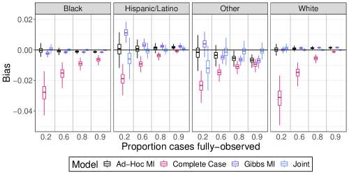
Figure 1: Bias across simulated datasets for the incidence, or $\mathbb{I}_{j}$ for Blacks, Hispanic/Latinos, Others, and Whites plotted against the proportion of cases observed with race data.

Bias in estimating incidence by race/ethnicity

As can be seen in Figure 1, for Blacks and Whites, which comprise 49% and 40% of the total population in Wayne County, the bias in the posterior mean incidence estimator generated by the joint model is small across all scenarios for most simulated datasets. For Whites, the average bias in the joint model posterior mean is not significantly different than zero in the 90%, 80% and 60% scenarios, while for Blacks, there is statistically significant average bias for joint-model posterior mean incidence in all scenarios other than 80%, but it is an order of magnitude smaller than the average bias of the posterior mean estimator from the imputation methods. The complete case model, as expected, is significantly negatively biased in all scenarios. The average bias from ad-hoc multiple imputation is smallest among all methods in the 20% scenario because the data generating process, outlined in Section 3.2, defines the true population rate of disease for each race/ethnicity group to be the same. The distribution of missing cases by category conditional on the total missing cases is multinomial with parameter $\mathbf{e}_{ig}\odot(1-\mathbf{p}_{ig})/\sum_{j}E_{igj}(1-p_{igj})$. When missingness is high, $(1-p_{igj})$ is close to one, so the ad-hoc multinomial imputation procedure with parameter $\mathbf{e}_{ig}/\sum_{j}E_{igj}$ is approximately correct. As missingness decreases, the ad-hoc imputation parameter diverges from the data generating process and the bias grows. This pattern can be seen in Figure 2 as well. In sum, the averages of the joint model estimators’ biases are sometimes more than two standard errors from zero, but the model’s absolute bias is significantly smaller compared to the absolute bias of the competing estimators, with exceptions in the 20% scenario compared to the Ad-Hoc MI method.

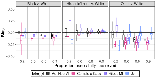
Figure 2: Bias across simulated datasets for the relative risk ratios, or $\mathbbm{I}_{j}/\mathbbm{I}_{J}$ for Blacks, Hispanic/Latinos, and Others relative to Whites plotted against the proportion of cases observed with race data.

Bias in estimating relative risk by race/ethnicity

In Figure 2 the joint model was able to estimate the relative risk of disease with mean bias that is not significantly different from zero for Blacks vs. Whites in the 80%, 60% and 20% observed scenarios, while in the 90% scenario the mean bias is significantly nonzero, but two orders of magnitude smaller than the mean bias incurred by the complete case model’s estimators. For Hispanic/Latinos and Others, there exists some mean bias in the 90%, 60%, and 20% scenarios, though in the 80% and 60% scenarios the mean bias is an order of magnitude smaller than that of the complete case analysis. Complete case analysis does yield estimators with average bias that is not significantly different from zero for the relative risk of disease for Hispanics/Latinos to Whites in the 90% observed scenario and has smaller average bias compared to the joint model’s estimators. This is due to the fact that in the simulated datasets the log-odds of observing race data was equal for Whites and Hispanics/Latinos, all else being equal. The average bias from multiple imputation using Gibbs sampling is consistently nonzero across all missingness scenarios for all groups in Figure 2. The Gibbs multiple imputation procedure assumes the data are MAR, when the DGP is NMAR for all scenarios. This highlights the danger of using a MAR procedure when the data are NMAR. The pattern of bias is similar for $\exp((\boldsymbol{\alpha}_{\lambda})_{j}-(\boldsymbol{\alpha}_{\lambda})_{J})$: the complete-case estimators are comparable in terms of mean bias to that of the joint-model estimators in the Hispanic/Latino group, while the complete-case estimators underperform in Blacks and Others. For $\boldsymbol{\sigma}_{\lambda}$, the complete-case posterior mean estimators are positively biased compared to the joint-model’s estimators, likely due to the fact that the complete case analysis attributes all variance in local area estimates of $\boldsymbol{\lambda}_{g}$ to variation in disease incidence while the joint model attributes some of the variation to variation in the observational process. The estimators from the joint model are, however, negatively biased, likely due to the fact that we have only 13 PUMAs and relatively strong $\text{Normal}^{+}(0,0.5^{2})$ priors that shrink towards zero on the population scale parameters $\boldsymbol{\sigma}_{\lambda}$.

Root mean squared error

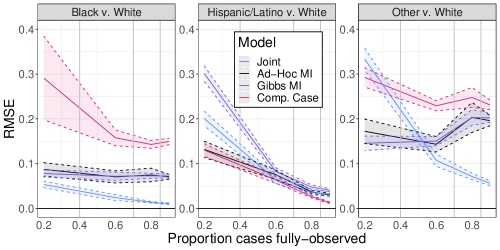
Figure 11: Root mean squared error across simulated datasets for the relative risk ratio, or $\mathbbm{I}_{j}/\mathbbm{I}_{J}$ for Blacks, Hispanic/Latinos, Others relative to Whites plotted against the proportion of cases observed with race data. The blue color corresponds to the joint model in equation (11), while the red color corresponds to a the model defined in equation (15), or a complete-case analysis. Smaller magnitude is better.

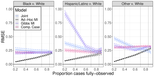
Figure 12: Mean squared error across simulated datasets for the population relative risk ratio, or $\exp((\boldsymbol{\alpha}_{\lambda})_{j}-(\boldsymbol{\alpha}_{\lambda})_{J})$ for Blacks, Hispanic/Latinos, Others relative to Whites plotted against the proportion of cases observed with race data. The blue color corresponds to the joint model in equation (11), while the red color corresponds to a the model defined in equation (15), or a complete-case analysis. Smaller magnitude is better.

The RMSEs are shown on in Section F.1. That of the joint-model estimators for $\text{SIR}_{j}$ are significantly smaller (as measured shown by nonoverlapping 95% confidence intervals) than the RMSEs for the complete-case estimators in the 90%, 80%, and 60% scenarios for nearly all groups (the exception is for Hispanics/Latinos in the 60% scenario, where the RMSEs are not significantly different). In the 20% observed scenario, the RMSEs of the joint-model estimators for Blacks and Whites are smaller than those of the complete case model, but the RMSEs of the joint-model estimators for Hispanic/Latinos and Others are larger than the complete-case estimators. This is due to the fact that Hispanic/Latinos and Others are smaller populations in Wayne County, and the parameter space for the is $2\times$ as large as the complete-case model’s parameter space. We also present the RMSE comparisons for the relative risk ratios and relative county-level rates, shown in figures 11 and 12, respectively. The relative risk ratio plots show a similar pattern to that of the $\text{SIR}_{j}$ estimates, with the exception of relative risk ratios for Hispanics/Latinos, for which the RMSEs of the complete-case estimators are smaller than those of the joint model’s. This is due to the fact that White and Hispanics/Latinos case-patients are observed at similar relative rates across simulations because the observation ratio, or $\text{inv\_logit}((\boldsymbol{\alpha}_{\eta})_{j})/\text{inv\_logit}((\boldsymbol{\alpha}_{\eta})_{J})=1$ for these two groups and the complete case analysis model implicitly assumes the observation ratios for all races to be exactly 1.

On the contrary, figure 12 shows that the RMSEs for the joint-model’s estimators are similar in magnitude or larger in all scenarios. While the joint-model’s estimators show smaller mean biases, the variance for the estimators is much larger compared to the complete case analysis. This is again due to the fact that there are only 13 PUMAs included in the simulation study, and the fact that the dimension of the parameter space is twice as large for the joint model as that of the complete case model. The RMSEs for the ad-hoc imputation approach are small in the 20% scenario for the same reason the bias is small in the 20% scenario, but the RMSE increases as the missingness decreases. This is a clear indication that the data generating process does not agree with the imputation procedure. The RMSEs for the Gibbs imputation approach are large for the 20% scenario, likely owing to the fact that as the number of missing cases increases, the variance of the imputed datasets increased due to increased posterior uncertainty for the imputation model. This could be an indication that more than 100 imputed datasets are necessary for the imputation procedure when missingness is high, which would accord with the observations in Zhou and Reiter (2010), though we were constrained by computational budget to use only 100 imputed datasets per simulated dataset.

3.6.3 Coverage and interval length

Table 3 summarizes the interval coverage for the complete-case model, the joint model, and the multiple imputation procedures. All intervals that follow are central $p\%$ posterior credible intervals. In the event the joint distribution of the simulated parameters and data matches the prior and the likelihood of the inferential model and we can properly draw samples from the posterior, the central $p\%$ posterior credible intervals (and any other posterior intervals, for that matter) will contain the parameter that generated the data with exactly $p\%$ probability (Cook, Gelman and Rubin, 2006). As expected, the complete-case model’s 50% intervals severely under cover for all but the county-level relative rates of disease for Hispanics and Latinos compared to the rate for Whites. The ad-hoc imputation method’s intervals over-covered for the population-level relative risk comparisons (as seen in 10), while they undercovered for the standardized incidence and relative risk measures, while the Gibbs sampler imputation’s intervals severely undercovered in all scenarios for all the parameters of interest. Despite the ad-hoc methods near-match to the data generating process in the 20% scenario, the intervals for incidence under-cover more than the joint model’s credible intervals. The joint model’s intervals are near the nominal coverage probabilities, i.e. the 50% intervals cover the true parameter value in 50% of simulations, though they do under-cover for sparsely populated groups like Others and Hispanic/Latinos, especially so with significant numbers of missing cases.

The same pattern is exhibited in the figure 3, which shows boxplots of the average coverage across all parameters related to the disease process for each simulated dataset for all models. The complete-case model’s 50% and 80% interval coverage is about 25% and 35%, respectively, while the joint model’s intervals achieve the nominal coverage probability on average. The multiple imputation methods’ intervals fare a bit better though they still under-cover: the rates are near 30%-35% and 60% to 65% on average.

In appendix section F.2 we present table 9, which mirrors table 3 but for 80% intervals. The pattern of performance is similar.

Table 3: Table shows 50% posterior credible interval coverages and lengths for estimands of interest from the simulation study. Coverage proportion is calculated across 200 simulated datasets for each model/simulation scenario. Column headers for percentages (e.g. 20%) indicate the missing-data simulation scenario which corresponds to the statistic calculated in the table column; the simulation scenario corresponds to the proportion of cases observed with completely observed race covariates.

		50% interval coverage				50% mean interval length
Parameter	Model	20%	60%	80%	90%	20%	60%	80%	90%
$\mathbbm{I}_{\text{Blacks}}$	Complete Case	0.00	0.00	0.00	0.00	1e-04	2e-04	2e-04	3e-04
	Joint	0.37	0.48	0.46	0.51	2e-03	7e-04	5e-04	4e-04
	Ad-Hoc MI	0.05	0.13	0.03	0.00	3e-04	3e-04	3e-04	3e-04
	Gibbs MI	0.01	0.01	0.00	0.00	5e-04	3e-04	3e-04	3e-04
$\mathbbm{I}_{\text{Hispanics/Latinos}}$	Complete Case	0.00	0.00	0.00	0.20	3e-04	5e-04	6e-04	7e-04
	Joint	0.26	0.47	0.48	0.42	6e-03	3e-03	2e-03	1e-03
	Ad-Hoc MI	0.07	0.15	0.18	0.00	9e-04	8e-04	8e-04	7e-04
	Gibbs MI	0.00	0.01	0.01	0.00	2e-03	1e-03	8e-04	7e-04
$\mathbbm{I}_{\text{Others}}$	Complete Case	0.00	0.00	0.00	0.00	3e-04	5e-04	5e-04	6e-04
	Joint	0.12	0.44	0.48	0.41	6e-03	5e-03	3e-03	3e-03
	Ad-Hoc MI	0.07	0.07	0.01	0.00	1e-03	8e-04	7e-04	7e-04
	Gibbs MI	0.09	0.01	0.00	0.00	2e-03	9e-04	7e-04	7e-04
$\mathbbm{I}_{\text{Whites}}$	Complete Case	0.00	0.00	0.00	0.00	1e-04	2e-04	3e-04	3e-04
	Joint	0.30	0.54	0.49	0.50	1e-03	7e-04	5e-04	4e-04
	Ad-Hoc MI	0.13	0.12	0.00	0.00	3e-04	3e-04	3e-04	3e-04
	Gibbs MI	0.14	0.01	0.00	0.00	4e-04	3e-04	3e-04	3e-04
$\mathbbm{I}_{\text{Blacks}}/\mathbbm{I}_{\text{Whites}}$	Complete Case	0.03	0.01	0.00	0.00	0.02	0.01	0.01	0.01
	Joint	0.48	0.54	0.52	0.48	0.06	0.03	0.02	0.01
	Ad-Hoc MI	0.04	0.10	0.01	0.00	0.01	0.01	0.01	0.01
	Gibbs MI	0.07	0.01	0.00	0.00	0.02	0.01	0.01	0.01
$\mathbbm{I}_{\text{Hispanics/Latinos}}/$	Complete Case	0.09	0.08	0.33	0.53	0.03	0.02	0.02	0.02
$\mathbbm{I}_{\text{Whites}}$	Joint	0.24	0.46	0.51	0.45	0.14	0.07	0.05	0.03
	Ad-Hoc MI	0.09	0.12	0.17	0.24	0.02	0.02	0.02	0.02
	Gibbs MI	0.00	0.09	0.07	0.05	0.05	0.02	0.02	0.02
$\mathbbm{I}_{\text{Others}}/\mathbbm{I}_{\text{Whites}}$	Complete Case	0.00	0.00	0.00	0.00	0.03	0.02	0.02	0.01
	Joint	0.12	0.43	0.47	0.41	0.16	0.12	0.09	0.07
	Ad-Hoc MI	0.09	0.06	0.00	0.00	0.02	0.02	0.02	0.02
	Gibbs MI	0.09	0.00	0.00	0.00	0.05	0.02	0.02	0.02

3.6.4 Breakdown analysis

The joint model performs well under the 90%-, 80%- and 60%-observed scenarios, but when there is a significant proportion of cases that are missing race data, like in the 20%-observed scenario, the model’s posterior intervals begin to undercover compared to the nominal coverage probabilities. One can see this in figure 3, as the interval coverage in the 60% observed scenario begin to undercover slightly as measured by the median across the 200 simulated datasets. In the 20% observed scenario, the $75^{\textrm{th}}$ quantiles of the mean parameter coverage for the full model for both the 50% and 80% intervals lie below the nominal coverage rates.

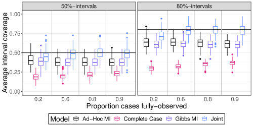
Figure 3: Boxplots of simulation-wise mean 50% and 80% interval coverage by observed data proportion scenario for the joint model, the complete-case model, and the multiple imputation methods. Horizontal black lines indicate the nominal coverage probability rates.

This leads us to conclude that informative priors are necessary when the model is fitted to datasets that have significant numbers of cases that are missing race data. If the likelihood and prior conflict, however, these priors may have an outsized influence on the posterior estimands.

3.7 Prior sensitivity results

In order to test the sensitivity of model inferences to priors over population hyperparameters such as the population mean log-incidence ($\boldsymbol{\alpha}_{\boldsymbol{\lambda}}$), or population mean log-odds of observing a specific race/ethnicity category ($\boldsymbol{\alpha}_{\boldsymbol{\eta}}$), we used a subset of 100 simulated datasets from the 20% observed scenario. We varied the parameters of the priors over the population hyperparameters over a grid and re-estimated the quantities of interest for each prior specification. We varied one prior parameter at a time while holding the other prior parameters fixed at the values shown in eq. 14. The parameter values are shown in Table 4.

Population parameter	Prior parameter	Values
${\boldsymbol{\alpha}_{\boldsymbol{\eta}}}_{j}$	$\mathbb{E}\left[\boldsymbol{\alpha}_{\boldsymbol{\eta}}\right]_{j}$	$\{0.5,1,\mathbf{2},3\}\forall j$
${\boldsymbol{\alpha}_{\boldsymbol{\lambda}}}_{j}$	$\mathbb{E}\left[\boldsymbol{\alpha}_{\boldsymbol{\lambda}}\right]_{j}$	$\{-3.5,-4,-4.5,\mathbf{-5}\}\forall j$
${\boldsymbol{\alpha}_{\boldsymbol{\eta}}}_{j}$	$\mathrm{SD}(\boldsymbol{\alpha}_{\boldsymbol{\eta}})_{j}$	$\{0.3,0.5,\mathbf{1},2,3\}\forall j$
${\boldsymbol{\alpha}_{\boldsymbol{\lambda}}}_{j}$	$\mathrm{SD}(\boldsymbol{\alpha}_{\boldsymbol{\lambda}})_{j}$	$\{0.3,0.5,\mathbf{1},2,3\}\forall j$
${\boldsymbol{\sigma}_{\boldsymbol{\eta}}}_{j}$	$\mathbb{E}\left[\boldsymbol{\sigma}_{\boldsymbol{\eta}}\right]_{j}/\sqrt{2/\pi}$	$\{0.25,0.5,\mathbf{1},2\}\forall j$
${\boldsymbol{\sigma}_{\boldsymbol{\lambda}}}_{j}$	$\mathbb{E}\left[\boldsymbol{\sigma}_{\boldsymbol{\lambda}}\right]_{j}/\sqrt{2/\pi}$	$\{0.25,0.5,\mathbf{1},2\}\forall j$

Table 4: Prior sensitivity simulation study prior settings.
Bold values correspond to settings used for results presented in 3.6. Prior parameter for $\boldsymbol{\sigma}_{\boldsymbol{\lambda}}$ and $\boldsymbol{\sigma}_{\boldsymbol{\eta}}$ is the standard deviation parameter for a half-normal distribution.

We measured 1) the sensitivity of the estimated posterior mean incidence by race/ethnic group, or $\mathbb{I}_{j}$, and 2) its bias. Our measure of posterior mean sensitivity to the prior mean was the change in posterior mean against a reference mean scaled by a reference standard deviation, where the reference mean and standard deviation were those obtained using the prior settings set out in Equation 14. Specifically, for an estimand $g(\boldsymbol{\theta})$, with a posterior over $\boldsymbol{\theta}$ $\pi_{\mathrm{b}}(\boldsymbol{\theta}|\mathrm{Data})$ under a prior with reference parameters $\mathrm{b}$ and a posterior $\pi_{\mathrm{a}}(\boldsymbol{\theta}|\mathrm{Data})$ under a prior with alternative parameters $\mathrm{a}$:

$$\text{Posterior Z-score}\,=\frac{\mathbb{E}_{\pi_{\mathrm{a}}(\boldsymbol{\theta}|\mathrm{Data})}[g(\boldsymbol{\theta})]-\mathbb{E}_{\pi_{\mathrm{b}}(\boldsymbol{\theta}|\mathrm{Data})}[g(\boldsymbol{\theta})]}{\sqrt{\mathrm{Var}_{\pi_{\mathrm{b}}(\boldsymbol{\theta}|\mathrm{Data})}(g(\boldsymbol{\theta}))}}$$ (16)

The measure of bias for a true estimand $g(\boldsymbol{\theta}^{\dagger})$ is

$$\frac{\mathbb{E}_{\pi_{\mathrm{a}}(\boldsymbol{\theta}|\mathrm{Data})}[g(\boldsymbol{\theta})]-g(\boldsymbol{\theta}^{\dagger})}{g(\boldsymbol{\theta}^{\dagger})}$$ (17)

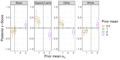
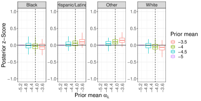
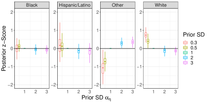
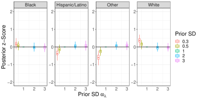
Figure 13: Graphs above show box plots of posterior-standard-deviation-scaled differences in posterior mean incidences with respect to a baseline prior for various priors over population hyperparameters, or $(\mathbb{E}_{\pi_{\mathrm{a}}(\boldsymbol{\theta}|\mathrm{Data})}[g(\boldsymbol{\theta})]-\mathbb{E}_{\pi_{\mathrm{b}}(\boldsymbol{\theta}|\mathrm{Data})}[g(\boldsymbol{\theta})])/{\sqrt{\mathrm{Var}_{\pi_{\mathrm{b}}(\boldsymbol{\theta}|\mathrm{Data})}(g(\boldsymbol{\theta}))}}$. The graphs quantify how sensitive posterior mean incidence for each race/ethnicity group is to priors over population parameters $\boldsymbol{\alpha}_{\boldsymbol{\lambda}}$ and $\boldsymbol{\alpha}_{\boldsymbol{\eta}}$.

Figure 13 shows that the posterior incidence estimate is somewhat sensitive to the priors over log-population mean incidence and log-odds of observing race/ethnicity information. The right-hand column in Figure 13 shows that as the prior mean for $\alpha_{\lambda}$ for the Other group differs from the true data-generating mean by 3 prior standard deviations, the posterior mean can change by roughly half a posterior standard deviation from the baseline prior.

Meanwhile, the left-hand column of Figure 13 shows the sensitivity of the posterior mean for incidence by race/ethnicity to the prior for $\alpha_{\lambda}$. Of interest is the posterior mean for the Other group because it is the minority group. In the $20$%-observed scenario, the true $\alpha_{\lambda}$ for the Other group is approximately $0.3$, while the prior mean for $\alpha_{\lambda}$ is $2$. When the prior standard deviation is decreased to 0.5 from 1, the prior mean is approximately 3 prior standard deviations away from the true data generating parameter, and the posterior mean decreases by about half a posterior standard deviation. Despite the fact that the posterior means can shift due to changes in the prior, however, the posterior mean never exceeds 2 posterior standard deviations, implying that the inferences do not appreciably change.

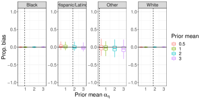
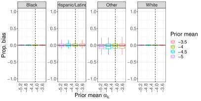
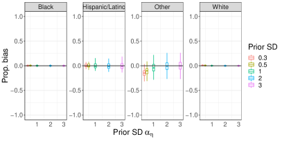
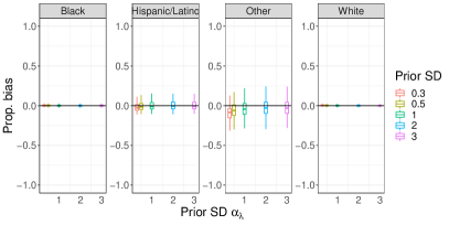
Figure 14: Graphs above show box plots of scaled biases in the posterior mean for true incidences $g(\theta^{\dagger})$, or $(\mathbb{E}_{\pi_{\mathrm{a}}(\boldsymbol{\theta}|\mathrm{Data})}[g(\boldsymbol{\theta})]-g(\boldsymbol{\theta}^{\dagger}))/{g(\boldsymbol{\theta}^{\dagger})}$. The graphs quantify how priors over population parameters $\boldsymbol{\alpha}_{\boldsymbol{\lambda}}$ and $\boldsymbol{\alpha}_{\boldsymbol{\eta}}$ influence the bias of the posterior mean estimator.

Digging deeper into the upper-left-hand plot in Figure 14 shows that when the prior for $\boldsymbol{\alpha}_{\boldsymbol{\eta}}$ is centered on missing-at-random missingness and the prior mean is too large compared to the true proportion of cases with observed race/ethnicity, the model over-allocates missing cases to majority groups while it under-allocates cases to minority groups. If we instead center the prior too low then we may over-allocate cases to minority groups.

The lower-left-hand plot in Figure 13 shows a similar phenomenon when the prior reflects too-strong certainty that the data-generating process is nearly missing-at-random. When too much prior weight is allocated to near-missing-at-random $\boldsymbol{\alpha}_{\boldsymbol{\eta}}$, the model deflates incidence for groups with higher-than-average missingness and inflates incidence for groups with lower-than-average incidence.

Figure 14 shows that the bias is not appreciable for incidence, with the exception of the Other group when the prior for $\alpha_{\lambda}$ is about 3 standard deviations or more too large.

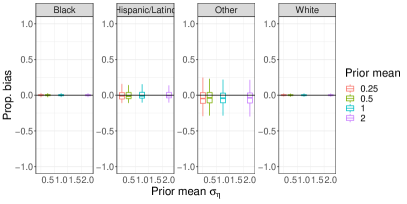
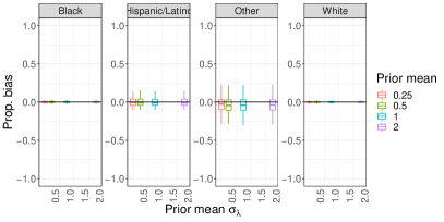
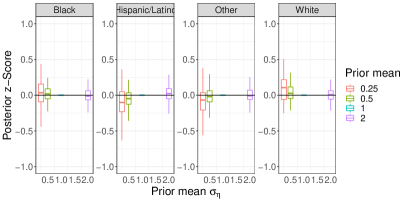
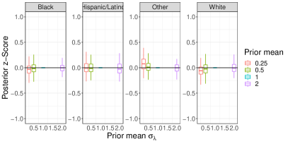
Figure 15: The graphs above show the posterior bias (eq. 17) and posterior z-scores (eq. 16) for $\boldsymbol{\sigma}_{\boldsymbol{\lambda}}$ and $\boldsymbol{\sigma}_{\boldsymbol{\eta}}$

Figure 15 shows posterior Z-score and bias plots for changes to the prior for population inter-geography standard deviation parameters for $\lambda_{gj}$ and $\eta_{gj}$, or $\boldsymbol{\sigma}_{\boldsymbol{\lambda}}$ and $\boldsymbol{\sigma}_{\boldsymbol{\eta}}$. The posterior for incidence is not especially sensitive to the prior over these parameters.

The results of the prior sensitivity simulation study show that the model inferences for incidence are relatively robust to misspecification of priors for population hyperparameters, but that care should be taken with the prior mass apportioned to data generating processes that are centered on missing-at-random scenarios.

4 Application to COVID-19 case data in Wayne County, Michigan

In this section we will apply both the complete-case model and the joint model to COVID-19 case data in Wayne County from the first wave of the pandemic.

4.1 Data

Table 5: Population summary in Wayne County, Michigan as of the 2010 Decennial Census

		Mean Age$\times$Sex$\times$Race/Eth.		$100\times$ Ratio
Race/Ethnicity	Total Pop.	$\times$PUMA Pop.	Std. dev. PUMA Pop.	to White
Asian/Pacific Islander	45894	196	315	5
Black	732801	3132	3152	81
Hispanic/Latino	95260	407	757	11
Other	44449	190	150	5
White	902180	3855	3225	100

Table 6: Cumulative incidence of PCR-confirmed COVID-19 infections in Wayne County, MI from March 1, 2020 through June 30, 2020. Mean and variance for Total uses only observed-race/ethnicity cases. Mean and Variance columns rounded to zero digits.

		Cumulative	Risk Relative			Prop. zero
Race/Ethnicity	Total Cases	Incidence	to Whites	Mean	Variance	counts
Asian/Pacific Islander	229	0.005	1.0	1	3	0.55
Black	9,577	0.013	2.6	41	1904	0.02
Hispanic/Latino	708	0.007	1.5	3	34	0.37
Other	834	0.019	3.8	4	13	0.18
White	4,476	0.005	1.0	19	389	0.08
Missing	3,464	NA	NA	15	204	0.06
Total	19,288	0.011	2.1	14	697	0.24

The source of our case data is the Michigan Disease Surveillance System (MDSS) maintained by the Michigan Department of Health and Human Services (MDHHS). MDHHS’s guidelines for the collection of probable COVID-19 cases is set out in Michigan Department of Health and Human Services. (2020) as outlined in Zelner et al. (2021). We included all reported PCR-confirmed COVID-19 cases for individuals outside of state prisons with that were entered into MDSS between $2020-03-01$ through $2020-06-30$. This comprises 22,141 cases of COVID-19. We then filtered out 1,374 cases, or about 6% of the total cases, that could not be geocoded to a unique address in Wayne County. We filtered a further 74 cases for which the case patients’ sex at birth was unknown, as well as 7 cases for which age was unknown. Finally, we dropped 1,398 cases which were matched to the address of a licensed nursing homes or long-term care facility (LTCF). We excluded these cases for two reasons: 1) the populations of nursing homes and LTCFs are likely not well-represented by the 2010 Census denominators and 2) the high incidence among nursing home and LTCF residents does not accord with our assumption of a Poisson process for disease cases. This results in a final dataset of 19,288 PCR-confirmed COVID-19 cases.

In total, approximately 18% of the 19,288 cases, or 3,464 cases, are missing race data. For cases that do include the race of the respondent and are not identified as Hispanic or Latino, we classify those who are identified as Asian or Hawaiian or Pacific Islander as Asian, those identified as Black/African American or Black/African American/Unknown as Black, and Caucasian and Caucasian/Unknown as White. We classify cases as Hispanic or Latino if the data field for patient ethnicity is equal to Hispanic or Latino. We classify those who identify as Native American or Alaska Native, mixed race, or other race as Other. Cases that are not missing race info but are missing patient ethnicity information are classified as the indicated race and are treated as not Hispanic or Latino.

We again have 13 PUMAs that comprise Wayne county, and 18 age by sex-at-birth strata per PUMA.

4.1.1 Aggregation to PUMAs

This yields 234 observations of the counts of PCR-confirmed COVID-19 cases within each race/ethnicity category, or 1,170 total observations of PUMA by age by sex-at-birth by race/ethnicity. The mean count is 13.5 while the variance is 696.9. As for observations of total counts of cases missing race and ethnicity information by PUMA by age by sex-at-birth, 6% of the 234 PUMAs have zero observed cases with missing race and ethnicity.

4.1.2 Population data

We added the Asian/Pacific Islander group as an additional race/ethnic category, because such individuals make up a significant fraction of the population in Wayne County, though in all other respects the PUMA-level population data is the same as in the simulation study in Subsection 3.1.

4.2 Models and priors

We fitted four of the models presented in Section 3.3: the joint model, the complete-case model, and the ad-hoc and Gibbs multiple imputation models. The full specification for the joint model is:

$$\begin{split}X_{igj}|\lambda_{gj},\mathbf{z}_{i},\boldsymbol{\beta}_{g},p_{igj},E_{igj}&\sim\text{Poisson}(p_{igj}\lambda_{gj}\exp(\mathbf{z}_{i}^{T}\boldsymbol{\beta}_{g})E_{igj}),\\ M_{ig}|\boldsymbol{\lambda}_{g},\mathbf{z}_{i},\boldsymbol{\beta}_{g},\mathbf{p}_{ig},\mathbf{e}_{ig}&\sim\text{Poisson}(\exp(\mathbf{z}_{i}^{T}\boldsymbol{\beta}_{g})\textstyle\sum_{j}((1-p_{igj})\lambda_{gj}E_{igj}),\\ p_{igj}&=\left(1+\exp(-(\mathbf{z}_{i}^{T}\boldsymbol{\gamma}_{g}+\eta_{gj})\right)^{-1},\\ \log\boldsymbol{\lambda}_{g}|\boldsymbol{\alpha}_{\lambda},\boldsymbol{\sigma}_{\lambda}&\sim\text{MultiNormal}(\boldsymbol{\alpha}_{\lambda},\text{diag}(\boldsymbol{\sigma}_{\lambda}^{2})),\\ \boldsymbol{\eta}_{g}|\boldsymbol{\alpha}_{\eta},\boldsymbol{\sigma}_{\eta}&\sim\text{MultiNormal}(\boldsymbol{\alpha}_{\eta},\text{diag}(\boldsymbol{\sigma}_{\eta}^{2})),\\ \boldsymbol{\beta}_{g}|\boldsymbol{\alpha}_{\beta},\boldsymbol{\sigma}_{\beta}&\sim\text{MultiNormal}(\boldsymbol{\alpha}_{\beta},\text{diag}(\boldsymbol{\sigma}_{\beta}^{2})),\\ \boldsymbol{\gamma}_{g}|\boldsymbol{\alpha}_{\gamma},\boldsymbol{\sigma}_{\gamma}&\sim\text{MultiNormal}(\boldsymbol{\alpha}_{\gamma},\text{diag}(\boldsymbol{\sigma}_{\gamma}^{2})),\end{split}$$ (18)

with the same priors over the hyperparameters as in eq. 14 with the exception of the prior scale for $\boldsymbol{\sigma}_{\gamma}$ set to $1$ instead of $0.5$.

The full specification for the complete-case model is

$$\begin{split}X_{igj}|\lambda_{gj},\mathbf{z}_{i},\boldsymbol{\beta}_{g},p_{igj},E_{igj}&\sim\text{Poisson}(\lambda_{gj}\exp(\mathbf{z}_{i}^{T}\boldsymbol{\beta}_{g})E_{igj}),\\ \log\boldsymbol{\lambda}_{g}|\boldsymbol{\alpha}_{\lambda},\boldsymbol{\sigma}_{\lambda}&\sim\text{MultiNormal}(\boldsymbol{\alpha}_{\lambda},\text{diag}(\boldsymbol{\sigma}_{\lambda}^{2})),\\ \boldsymbol{\beta}_{g}|\boldsymbol{\alpha}_{\beta},\boldsymbol{\sigma}_{\beta}&\sim\text{MultiNormal}(\boldsymbol{\alpha}_{\beta},\text{diag}(\boldsymbol{\sigma}_{\beta}^{2})),\end{split}$$ (19)

with the same priors as the joint model over the shared hyperparameters $\boldsymbol{\alpha}_{\lambda},\boldsymbol{\alpha}_{\beta},\boldsymbol{\sigma}_{\lambda}$ and $\boldsymbol{\sigma}_{\beta}$.

$\mathbf{z}_{i}$ was $9$-dimensional, with the first element encoding male vs. female and the next eight elements encoding the age stratum from $[0,10)$ to $[70,80)$. We used a sum contrast for age and a scaled sum contrast for male vs. female. We used the results of Theorem 2.2 to check that our model as defined is locally identifiable for each PUMA. All 13 PUMAs meet our criteria for the model to be locally identifiable. We needed to rerun the identifiability analysis because we expanded our race/ethnicity categories by one to include Asians/Pacific Islanders as a separate group. Our construction of the $\boldsymbol{\beta}_{g}$ and $\boldsymbol{\gamma}_{g}$ is the same as in the simulation study.

4.2.1 Computational results

We again used cmdstanr as the Stan interface via R (Gabry and Češnovar, 2021; R Core Team, 2021b). Each model was run with 8 MCMC chains with 3,000 warmup iterations, and 2,000 post-warmup iterations with a target Metropolis acceptance rate of 0.99. For the joint model, all $\hat{R}$s were less than 1.01, while the minimum bulk and tail ESS efficiencies were 0.098 and 0.200 rounded, respectively. For the complete-case model, all $\hat{R}$s were less than 1.01, while the minimum bulk and tail ESS efficiencies were 0.156 and 0.238, respectively. All ESS efficiency numbers are rounded to three digits.

The multiple imputation methods were run for 1,000 warmup, and 2,000 post-warmup iterations for each of the 100 imputed datasets. All $\hat{R}$s were below 1.01 for each imputed datasets MCMC run, and minimum bulk and tail efficiencies exceeded 10% for the Gibbs imputation scheme while minimum bulk and tail efficiencies exceed 9% and and 10%, respectively for the ad-hoc imputation scheme. Note that the $\hat{R}$ statistics for the combined chains are typically larger than 1.01 for many parameters of interest, which can be seen in table 12. This is due to the between-imputed-dataset variance.

4.3 Results and Model Comparison

4.3.1 Comparison of model results on completely-observed cases

Following Gelman et al. (2020) and Gabry et al. (2019), we performed a series of graphical posterior predictive checks, or PPCs, using the bayesplot package (Gabry and Mahr, 2021). These involved simulating PUMA by age by sex by race case counts from the fitted models and comparing these outputs to the observed data. Along this dimension, the joint model and the complete-case model were indistinguishable in terms of errors, squared errors, and 50%, 80% and 95% interval coverage for the observed data.

These checks also revealed that the observational variance, or $\frac{1}{IJ-1}\sum_{i,j}(x_{ij}-\bar{x})^{2}$, $\bar{x}=\frac{1}{IJ}\sum_{i,j}x_{ij}$ and the proportion of zeros, or $\frac{1}{IJ}\sum_{i,j}\mathbbm{1}_{x_{ij}=0}$, fell near the $50^{\textrm{th}}$ percentile for each model’s posterior over the two statistics, which indicates that the Poisson distribution is a suitable outcome distribution for this dataset.

We also used graphical PPCs to gauge whether the model assumption that there is no interaction between race and age is reasonable. The plots are included in Appendix Section H.1, and show that while there were deviations from the model’s posterior distribution for age by race cumulative incidence, they are small compared to the total cumulative incidence. Moreover, our interest lies in quantifying cumulative incidence by race for Wayne county instead of capturing all sources of variation in the observed data.

4.3.2 Posterior predictive checks on missing cases

We can compare the observed statistics for the missing cases to the joint model’s posterior predictive distribution for the same statistics. The mean, variance, and proportion of age/race/sex strata with zero cases observed all fell well within the joint model’s central 50% posterior intervals. A posterior predictive rootogram shown in Appendix Section H.2 that the tail is a bit thicker than the joint model expects, but the deviation is not extreme enough to warrant modifying the model.

4.3.3 Inference on epidemiological estimands

Following the results of our simulation study, the models’ inferences differed for the estimands introduced in Subsection 3.4, like modeled incidence, standardized incidence, standardized incidence ratios, and functions of these estimands.

A comparison of the modeled incidence inferences for the joint model, the complete-case model, and the Gibbs-sampler-imputation method is shown in Figure 4. The most striking aspect of the figure is the elevated incidence in the Other race category across all methods. The complete case model infers uniformly lower incidence than does the joint model, which makes sense as the complete case model omits cases that are missing race/ethnicity information. The left-hand panel shows the Gibbs-imputation method imputes higher incidence for Whites, Asians/Pacific Islanders, and Hispanics/Latinos compared to the joint model. This mirrors the Gibbs performance in the simulation study as shown in Figure 5. The plot shows that the standardized difference in posterior means between the Gibbs imputation and the joint model is systematically greater than zero for Hispanic/Latinos and Whites, while it is systematically lower than zero for Others in the 80% observed data scenario. Visually, we can see that the understatement for incidence is more extreme for Blacks and Others than it is for Hispanics or Latinos and for Whites. Both the Gibbs and complete case intervals are shorter than the joint-model intervals.

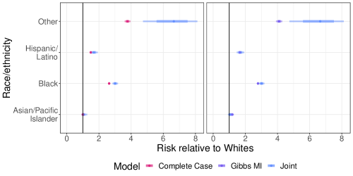
Figure 8: Relative risk of COVID-19. The inner intervals are 50% and the outer intervals are 80%.

Figure 8 shows the relative modeled incidence, or $\mathbb{I}_{j}/\mathbb{I}_{J}$, where $J$ is the category for Whites. The plot shows that relative risks for all nonwhites are smaller when using complete case analysis compared to that of the joint model. The increase is most substantial for the Other race/ethnicity category, but both Blacks and Hispanic and Latinos have significant increases in relative risk.

Table 11 in Appendix Subsection H.3 shows the exhaustive comparison between the two models for all of the estimands. Despite the models showing statistically significant differences for posterior means among the standardized incidence ratios, the practical differences are small for Blacks, Hispanics and Latinos and Asians and Pacific Islanders. The 80% posterior credible intervals, on the contrary, are larger on average for the joint models’ inferences on the standardized incidence ratios. Whites and people of Other races are seen to have statistically significant and practically significant differences in the models’ posterior mean estimators. The models’ inferences differed most significantly in terms of relative incidence, as can also be seen in Figures 8, where for Blacks vs. Whites and Others vs. Whites the posterior 80% credible intervals do not overlap, even after taking into account Monte Carlo standard error. The joint model’s posterior intervals for the epidemiological parameters of interest were wider on average, in agreement with the simulation study results.

4.3.4 Inference on missingness parameters

We cannot directly compare the inferences for the missingness parameters for the complete-case model to the joint model. We can, however, examine how the ratio of modeled incidences by race differs between races. In Figure 6, one can see that the 80% posterior credible intervals for the ratio of the complete-case model’s incidence to the joint model’s incidence do not include 1 for all races other than Asians and Pacific Islanders. The only groups for which the ratio of Gibbs-to-joint-model incidences exclude zero are Whites and Others, which again mirrors the pattern in Figure 5, though the difference is less extreme for Hispanics/Latinos and Asians/Pacific Islanders for the real-world data. The Gibbs imputation method’s inference for Blacks nearly matched that of the joint model. This is not surprising when we consider the fact that between-group comparisons of the ratio of incidences reveals that non-White residents, excluding Others had missingness proportions that were near equal between groups. This can be seen from 6 as the posterior intervals for the Complete Case comparison overlap for Hispanics/Latinos, Blacks and Asian/Pacific Islanders. It can also be seen that the posterior intervals for Others do not overlap with any other category, and that Whites and Blacks are also do not overlap. Figure 7 shows the supporting evidence for NMAR missingness of race; the plot shows the Wayne-County-wide population inferences for the probability that an individual with COVID-19 of a certain race will have race reported in their case line-listing, all else being equal. This estimand is a transformation of the $\boldsymbol{\alpha}_{\eta}$ parameter, namely, $\text{inv\_logit}(\boldsymbol{\alpha}_{\eta})$. The strongest evidence for NMAR missingness exists for the Other category, whose 80% posterior credible intervals do not intersect any other category’s intervals. There is also some evidence for NMAR missingness for Blacks with respect to Whites, as the 80% posterior credible intervals for the probability of completely observing race are $(0.81,0.91)$ vs. $(0.89,0.98)$, respectively, as shown in Table 13 in Appendix Subsection H.3.

Figure 4: Race/ethnicity category-specific modeled incidence by model. The inner intervals are 50% and the outer intervals are 80%.

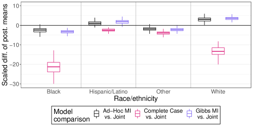
Figure 5: Boxplots of differences in posterior means between indicated methods and joint model scaled by pooled posterior standard deviation by race/ethnicity category-specific modeled incidence by simulated dataset for the 80% observed data scenario.

4.3.5 Summary

Our results largely align with those of prior analyses of racial disparities in COVID-19 incidence in the U.S. For example, Labgold et al. found a similarly large incidence among case-patients of Other race. The authors find a bias-adjusted PCR-confirmed COVID-19 rate of nearly 14% among Other race case-patients compared to rates of at most nearly 4% in Hispanic/Latino case-patients, who had the next-largest incidence among the races included in Labgold et al.’s study. The relative incidence between Others and Whites is nearly 14, which puts our 80% posterior credible interval of $(4.77,8.11)$ in context.

Several explanations are plausible for the elevated incidence among people of Other races; Wayne county has a large Middle Eastern population and these individuals may identify themselves as not being Black, Hispanic or Latino, Asian or Pacific Islander or White. The case data does include a field for Arab ethnicity, but the 2010 Census did not include a Middle Eastern or North African category for ethnicity. Another explanation may be our treatment of missing Hispanic/Latino ethnicity information. If many people who are identified as Other but do not have a recorded Hispanic/Latino ethnicity are truly Hispanic/Latino then our model would inflate the incidence in the Other category at the expense of the Hispanic/Latino category; given that the Other group is so small a small inflation in counts would result in a large inflation of risk.

There is strong evidence for nonignorable missingness driven by not-missing-at-random race covariates. The evidence is strongest for people of Other races. This means that omitting cases that are missing race and calculating relative risk between any race and Other would yield a biased estimate. Moreover, the size of the bias would be large because the probability of observing race for Others is low compared to the other categories; the 80% posterior credible interval is $(0.45,077)$. There is also some evidence for NMAR missingness for Blacks with respect to Whites. Given the small number of PUMAs we modeled, there would likely be stronger evidence in favor of NMAR missingness for other race/ethnicity categories if we were to model a larger geographical area, like all of Southeastern Michigan instead of just modeling Wayne County.

While the Complete Case inferences are predictably different from the joint model’s, the multiple imputation using Gibbs sampling also produced significantly different inferences. The coherence between the simulated data example and the applied data analysis suggest that multiple imputation procedures that assume MAR missingness when data are NMAR can exacerbate biases in the data by over-imputing cases for groups that are over-represented in the data because of NMAR missingness. This suggests that care must be taken when choosing an imputation procedure for missing demographic data.

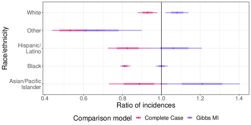
Figure 6: Posterior credible intervals for the ratio of modeled incidences by race/ethnicity, or $\mathbb{I}^{\text{CC}}_{j}/\mathbb{I}^{\text{J}}_{j}$ where CC stands for complete case model and $J$ stands for the joint model. The inner and outer intervals are 50% and 80% respectively.

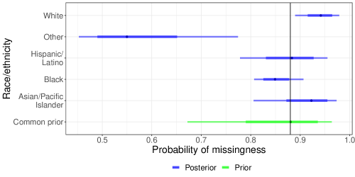
Figure 7: Posterior credible intervals for the population proportion of cases with fully-observed race data, all else being equal, by race/ethnicity, or $\text{inv\_logit}((\boldsymbol{\alpha}_{\eta})_{j})$. The inner and outer intervals are 50% and 80% respectively.

Overall, our case study illustrates the large risk of bias associated with ignoring NMAR categorical data when inferring relative risks from real-world data.

5 Discussion

Non-random missingness of race/ethnicity covariate data is a critical challenge for the analysis of public heath data during the COVID-19 pandemic. Multiple imputation methods, which have been adopted broadly in the analysis of survey data in which the assumption of ignorability is typically reasonable (Audigier et al., 2018), may not be appropriate for the analysis of missing race/ethnicity covariates in public health surveillance data in which the possibility of not-missing-at-random (NMAR) missingness is greater.

In order to meet the needs of public health researchers to model disease data that are missing important covariates, we developed a method to jointly model the missingness process along with the disease process. Most importantly, the model can learn the extent to which the missingness process is NMAR, so our method is broadly applicable to scenarios where missingness could plausibly be NMAR, like that of missing race data.

We use a selection model formulation that combines a Poisson sampling model for the counts of disease by stratum and a conditional binomial sampling model for cases with completely observed race/ethnicity with a probability of success parameter that depends on the race/ethnicity category. Through the incorporation of known population counts from census data, the model parameters can be identified. The model can be extended to incorporate a log-linear model for incidence, a logistic model for missingness, and a hierarchy to allow for geographic heterogeneity in local parameters.

Our use case is focused on missing race data in COVID-19 cases in Wayne County, Michigan from March 2020 through June 2020, which we suspect may have been NMAR. Wayne county saw the largest share of PCR-confirmed COVID-19 cases in the first wave of the pandemic, and also had a large share of cases that were missing race data, so it makes for an appropriate test bed for our method.

We ran a simulation study using Wayne county as the setting where we varied the proportion of cases with observed race from as high as 90% to as low as 20% to quantify the joint model’s finite sample performance and to compare its performance against a complete-case analysis and two multiple imputation methods. The results showed that the joint model performed well in the 90%- through 40%-observed scenarios compared to the competing methods though its performance suffered in the 20% observed-data scenario. This leads us to conclude that in order to use the joint model effectively in sparse data scenarios, better priors will be needed; prior formulation for the model is an area of active research.

We then applied the models to a dataset comprising PCR-confirmed COVID-19 cases with incomplete race data from Wayne County between March 2020 through June 2020. The differences between the joint-model inferences and the multiple-imputation inferences suggest that the missingness process for race may be NMAR and that care must be taken when applying methods that assume data are MAR. Model results also suggest that cases in the Other category, which comprises those of mixed race, Native Americans, and Other races, are being undercounted in Wayne County.

5.1 Limitations

The biggest limitation of our analysis is the result of the joint model’s dependence on census data for identifiability. This required the use of 2010 Decennial Census data, which is 10 years old, and may be systematically different than the true population distribution in Wayne County in 2020. The 2010 Decennial Census, however, is the most up-to-date source of spatially detailed population information, reflecting a broader limitation of any analysis that is dependent on decennial census data to estimate infection rates and relative risks. Because of this dependence on census population data, we were unable to model risk for race/ethnic categories that were potentially important in the Wayne County COVID-19 dataset, but for which census data were not available. MDSS collected information on Hispanic/Latino ethnicity separately from race, which resulted in missing covariate information in both categorical variables. Ideally we would have applied our method to multiple categorical covariates with missingness, but we were prevented from doing so due to the Census’ coarse race and ethnicity categories. As stated in Section 3.1, if the Census recorded ethnicity and race separately, we would be able to model the effect of ethnicity separately from that of race and we could treat the missing ethnicity data separately from that of missing race data. Instead, we set race/ethnicity as being equal to the observed race if Hispanic/Latino ethnicity was missing, which can understate uncertainty in our posterior and could result in understating incidence for Hispanics and Latinos and overstating incidence in all other categories. We ran a separate analysis where we treated these observations as missing race; the incidence results largely agreed with the model we presented in the main text for Blacks, Latinos, and Asians, though we observed significant differences in the White and Other incidences. This analysis overstates uncertainty, because individuals for whom we observe race but not ethnicity can be only one of two categories, but our model in its current formulation treats these cases as potentially arising from any of the race/ethnicity categories. Until we have detailed 2020 Decennial Census results, we cannot model ethnicity and race separately.

We are also constrained by the mismatch of the 2010 Census question about sex and our dataset’s definition of sex at birth. As Kennedy et al. (2020) argues, responses to the U.S. Census’ question of sex may not correspond to sexes at birth. This mismatch can lead to bias in our parameter estimates and an understatement of uncertainty.

Another limitation of our model is that it assumes a Poisson sampling distribution for incident cases of disease. When cumulative incidence increases over time, as has occurred with COVID-19, a binomial sampling model may be more appropriate. Similarly, our model assumes conditional independence between disease counts, which may not be appropriate as cumulative incidence grows. Both of these reasons are why we decided to focus on the first wave of the pandemic, which is when the disease was relatively rare among the population of Wayne County and for which the violations of conditional independence assumption could be reasonably assumed to not lead to too much understatement of uncertainty.

5.2 Conclusion

Public health surveillance systems will always have to contend with missing data. Because the nature and causes of this missingness are likely to change over time and across disease systems, it is important that the methods used to address missingness are flexible and able to account for both MAR and NMAR covariates. In Michigan, missingness of categorical demographic data among COVID-19 cases has varied over the course of the pandemic. For example, some localities in our data reported as much as 40% of PCR-confirmed COVID-19 cases having missing data on race/ethnicity for the period of rapidly-increasing incidence from October 2020 to February 2021.

Our simulation study shows that complete-case analysis or naïve multiple imputation can yield uncertainty intervals that are too short to be useful and point estimators that can over- or under-state between-group relative risks. Our method represents a computationally tractable and analytically transparent alternative that performs well in many scenarios, as evidenced in our simulation studies as well as analysis of data from Wayne County, Michigan.Given the need for public health authorities to characterize risks of disease among different population groups in as close to real-time as possible, flexible, efficient methods such as ours, are urgently needed.

5.2.1 Extensions and future work

This work can serve as a foundation on which to build new joint-disease-missing-covariate models targeted to specific applications. Although the model presented here can give useful inferences in its own right in a variety of settings, despite its relative simplicity, domain-specific modifications may be appropriate. For example, future models could incorporate multi-level information on the public health and healthcare systems generating surveillance data to account more explicitly for contextual drivers of missingness.

The joint model can also be extended to account for infectious disease transmission dynamics and other sources of temporal and spatial autocorrelation. For example, the one-period Poisson sampling model can be extended to a time-series susceptible-infected-recovered (TSIR) model or an endemic/epidemic model, both of which are discrete time analogues to classical susceptible-infected-recovered models (Held and Paul, 2012; Meyer and Held, 2014; Wakefield, Qi Dong and Minin, 2019; Bauer and Wakefield, 2018; Keeling and Rohani, 2011). When the disease becomes more widespread, potentially requiring a binomial likelihood, modeling the data a finer spatial resolution would make integrating over non-Poisson random variables more computationally efficient, particularly when combined with parallel computation of the likelihood. A dynamic programming implementation of the likelihood using binomial- instead of Poisson-distributed disease counts is included in appendix I. In order to regularize the model’s inferences as the parameter space dimension increases in step with the spatial resolution, one can use a computationally-efficient log-Gaussian Cox process as a prior for the spatially-dependent parameters (Li et al., 2012; Simpson et al., 2016). Furthermore, relaxing the conditional independence between categories is possible through a latent Poisson model, which we leave for future work.

The dependence of the joint model on the availability of sufficiently detailed and recent census data can also be mitigated. For example, uncertainty in group-specific population denominators can be accounted using frequently updated population datasets, such as the American Community Survey, even if these data are not available at the same level of spatial granularity as decennial census data. An alternative route is to perform a “tipping point” sensitivity analysis (Liublinska and Rubin, 2014) to flag changes in census data that would lead to a substantive change in conclusions (e.g. a reversal of the sign for log relative-risk measures). Given the many degrees-of-freedom of census population data, and the critical role played by such data in population-based analyses of health and illness, this presents an interesting and important challenge that should be explored in future work.

Appendix A Selection model derivation

Following Little, Rubin and Zangeneh (2017) and Gelman et al. (2013), we wish to model the joint distribution for the data:

$$\prod_{(i,j)}f((y_{ij},x_{ij})|\mu_{ij},p_{ij})$$

which we have factorized according to a selection model paradigm: $f(y_{ij}|\mu_{ij})$, and $f(x_{ij}|y_{ij},p_{ij})$, which follows from the conditional independence across $i$ and $j$ assumed in the generative model above. Let the vectors $\boldsymbol{\mu}_{i}$, $\mathbf{p}_{i}$ be the $J$-vectors with respective $j^{\textrm{th}}$ elements $\mu_{ij}$ and $p_{ij}$. Let $x_{ij}$, $w_{ij}$, $m_{i}$ be a specific realizations of $X_{ij}$, $W_{ij}$, $M_{i}$ and let $\mathbf{x}_{i}$, $\mathbf{w}_{i}$ be defined as $\boldsymbol{\mu}$ was defined, and where $W_{ij}\coloneqq Y_{ij}-X_{ij}$. Let $\mathbf{m}$ be the $I$ vector with $i^{\textrm{th}}$ element $m_{i}$. Then the complete data likelihood is defined as:

$$L((\boldsymbol{\mu}_{1},\mathbf{p}_{1}),\dots,(\boldsymbol{\mu}_{I},\mathbf{p}_{I}) |(\mathbf{x}_{1},\mathbf{w}_{1}),\dots,(\mathbf{x}_{I},\mathbf{w}_{I}))$$

$$=\int\prod_{(i,j)}e^{-\mu_{ij}}\frac{\mu_{ij}^{y_{ij}}}{y_{ij}!}\frac{y_{ij}!}{x_{ij}!w_{ij}!}p_{ij}^{x_{ij}}(1-p_{ij})^{w_{ij}}d\mathbf{w}_{1}\dots d\mathbf{w}_{I}$$

which is shown in appendix B to be

$$L((\boldsymbol{\mu}_{1},\mathbf{p}_{1}),\dots,(\boldsymbol{\mu}_{I},\mathbf{p}_{I}) |(\mathbf{x}_{1},m_{1}),\dots,(\mathbf{x}_{I},m_{I}))$$

$$=\left(\prod_{(i,j)}e^{-p_{ij}\mu_{ij}}\frac{(p_{ij}\mu_{ij})^{x_{ij}}}{x_{ij}!}\right)\prod_{i}e^{-\sum_{j}(1-p_{ij})\mu_{ij}}\frac{(\sum_{j}(1-p_{ij})\mu_{ij})^{m_{i}}}{m_{i}!}$$

By the properties in Little, Rubin and Zangeneh (2017) and Gelman et al. (2013) if $p_{ij}\neq p_{i}\forall(i,j)$ the complete data likelihood does not factorize into a term governing the observational process in $Y$ and the missinginess process in $R$, viz.

$$L(( \boldsymbol{\mu}_{1},\mathbf{p}_{1}),\dots,(\boldsymbol{\mu}_{I},\mathbf{p}_{I})|(\mathbf{x}_{1},m_{1}),\dots,(\mathbf{x}_{I},m_{I}))\neq$$

$$L(\boldsymbol{\mu}_{1},\dots,\boldsymbol{\mu}_{I}|(\mathbf{x}_{1},m_{1}),\dots,(\mathbf{x}_{I},m_{I}))L(\mathbf{p}_{1},\dots,\mathbf{p}_{I}|(\mathbf{x}_{1},m_{1}),\dots,(\mathbf{x}_{I},m_{I}))$$

Given that equality does not hold when $p_{ij}$ vary by $j$, we can say that in this case the data are not missing at random (NMAR), and thus we must model the joint distribution of observed data and missing data.

The observed data likelihood above is equivalent to the following generative model for the observed random variables $X_{ij}$ and $M_{i}$:

$$\begin{split}X_{ij}|p_{ij}\mu_{ij}&\sim\text{Poisson}(p_{ij}\mu_{ij})\\ M_{i}|\boldsymbol{\mu}_{i},\mathbf{p}_{i}&\sim\text{Poisson}(\textstyle\sum_{j}\mu_{ij}(1-p_{ij}))\end{split}$$ (20)

If we observe data for more than one geographic area, say for $g\in\{1,\dots,G\}$, we might expect our parameters to vary across locations. For example, geographic heterogeneity in cumulative incidence has been a fundamental characteristic of the COVID-19 pandemic and many other infectious disease outbreaks and epidemics (Bilal et al., 2021; Wakefield, Qi Dong and Minin, 2019). We can extend our generative model to capture geographic variation if we index our parameters with $g$ and model them as jointly distributed under $F_{\boldsymbol{\phi}}$, with $\boldsymbol{\phi}$ as a vector of unknown hyperparameters:

$$((\boldsymbol{\mu}_{1g},\mathbf{p}_{1g}),\dots,(\boldsymbol{\mu}_{Ig},\mathbf{p}_{Ig}))|\boldsymbol{\phi}\sim F_{\boldsymbol{\phi}}\ ,\forall g,$$ (21)

where $\boldsymbol{\mu}_{ig}$ and $\mathbf{p}_{ig}$ are $J$-vectors where the $j^{\textrm{th}}$ elements are equal to $\mu_{igj}$ and $p_{igj}$, respectively. The observed data model becomes

$$\begin{split}X_{igj}|p_{igj}\mu_{igj}&\sim\text{Poisson}(p_{igj}\mu_{igj}),\\ M_{ig}|\boldsymbol{\mu}_{ig},\mathbf{p}_{ig}&\sim\text{Poisson}(\textstyle\sum_{j}\mu_{igj}(1-p_{igj})),\end{split}$$ (22)

By extension, the joint hierarchical likelihood is:

$$\begin{split}\prod_{g}\big{(}&L((\boldsymbol{\mu}_{1g},\mathbf{p}_{1g}),\dots,(\boldsymbol{\mu}_{Ig},\mathbf{p}_{Ig})|(\mathbf{x}_{1g},m_{1g}),\dots,(\mathbf{x}_{Ig},m_{Ig}))\\ &f((\boldsymbol{\mu}_{1g},\mathbf{p}_{1g}),\dots,(\boldsymbol{\mu}_{Ig},\mathbf{p}_{Ig})|\boldsymbol{\phi})\big{)}\end{split}$$ (23)

where $f((\boldsymbol{\mu}_{1g},\mathbf{p}_{1g}),\dots,(\boldsymbol{\mu}_{Ig},\mathbf{p}_{Ig})|\boldsymbol{\phi})$ is the density associated with $F_{\boldsymbol{\phi}}$.

In the context of the COVID-19 case data, one might focus their analysis on a single county comprised of many smaller spatial units, with county-level parameters the target of inference, as in (23) and (21) as $\boldsymbol{\phi}$. We will typically have prior information about the hyperparameters from data in other states or in nearby counties, so we opt to use Bayesian inference. If we represent the prior density for $\boldsymbol{\phi}$ as $h(\boldsymbol{\phi}|\boldsymbol{\tau})$ and $\boldsymbol{\tau}$ are known, the joint posterior is:

$$\begin{split}\pi(&(\boldsymbol{\mu}_{1g},\mathbf{p}_{1g}),\dots,(\boldsymbol{\mu}_{Ig},\mathbf{p}_{Ig}),\boldsymbol{\phi}\big{|}(\mathbf{x}_{1g},m_{1g}),\dots,(\mathbf{x}_{Ig},m_{Ig}))\propto\\ \big{(}\prod_{g}\big{(}&L((\boldsymbol{\mu}_{1g},\mathbf{p}_{1g}),\dots,(\boldsymbol{\mu}_{Ig},\mathbf{p}_{Ig})|(\mathbf{x}_{1g},m_{1g}),\dots,(\mathbf{x}_{Ig},m_{Ig}))\\ &f((\boldsymbol{\mu}_{1g},\mathbf{p}_{1g}),\dots,(\boldsymbol{\mu}_{Ig},\mathbf{p}_{Ig})|\boldsymbol{\phi})\big{)}\big{)}h(\boldsymbol{\phi}|\boldsymbol{\tau})\end{split}$$ (24)

Given the structure of the model, the marginal posterior for $\boldsymbol{\phi}$ is informed by the data via the terms $L((\boldsymbol{\mu}_{1g},\mathbf{p}_{1g}),\dots,(\boldsymbol{\mu}_{Ig},\mathbf{p}_{Ig})|(\mathbf{x}_{1g},m_{1g}),\dots,(\mathbf{x}_{Ig},m_{Ig}))$, so it is important to understand the characteristics of the likelihood.

It can be seen that neither (20) nor (22) is identifiable as written without further assumptions.

Appendix B Derivation of likelihood in Section 2

Here we give proof of the following property used in Section 2: the data generating model given by the Poisson process and Binomial selection process at the beginning of Section 2 results in model (20).

Consider two groups, $j\in[1,2]$. As above, our fully observed likelihood gives the density for the vector of random variables, $(X_{i1},X_{i2},W_{i1},W_{i2})\forall i$, while we observe only $(X_{i1},X_{i2},M_{i})\forall i$. Thus, we must integrate over the set of all $\{(W_{i1},W_{i2}|W_{i1}+W_{i2}=M_{i}\}$.

$$\Pb\left(X_{i1}=x_{i1},X_{i2}=x_{i2},M_{i}=m_{i}\right)=$$ (25)

$$\Pb\left((X_{i1}=x_{i1},W_{i1}=0),(X_{i2}=x_{i2},W_{i2}=0)\right)\mathbbm{1}(m_{i}=0)$$ (26)

$$+\sum_{e=0}^{m_{i}}\Pb\left((X_{i1}=x_{i1},W_{i1}=e),(X_{i2}=x_{i2},W_{i2}=(m_{i}-e)\right)\mathbbm{1}(m_{i}>0).$$ (27)

Given that $W_{ij}=Y_{ij}-X_{ij}$, this expression is equivalent to

$$\Pb\left((X_{i1}=x_{i1},Y_{i1}=x_{i1}),(X_{i2}=x_{i2},Y_{i2}=x_{i2})\right)\mathbbm{1}(m_{i}=0)$$ (28)

$$+\sum_{e=0}^{m_{i}}\Pb\left((X_{i1}=x_{i1},Y_{i1}=x_{i1}+e),(X_{i2}=x_{i2},Y_{i2}=x_{i2}+(m_{i}-e)\right)\mathbbm{1}(m_{i}>0).$$ (29)

Each term

$$\Pb\left((X_{i1}=x_{i1},Y_{i1}=y_{i1}),(X_{i2}=x_{i2},Y_{i2}=y_{i2})\right)$$

decomposes to

$$\Pb\left(X_{i1}=x_{i1}|Y_{i1}=y_{i1}\right)\Pb\left(Y_{i1}=y_{i1}\right)\Pb\left(X_{i2}=x_{i2}|Y_{i2}=y_{i2}\right)\Pb\left(Y_{i2}=y_{i2}\right)$$

given the independence between $Y_{i1}$ and $Y_{i2}$ and the conditional independence of $X_{i1}|Y_{i1}$ and $X_{i2}|Y_{i2}$.

$$\prod_{i=1}^{I}\left(\frac{\lambda_{i1}^{x_{i1}}e^{-\lambda_{i1}}}{x_{i1}!}p_{i1}^{x_{i1}}\frac{\lambda_{i2}^{x_{i2}}e^{-\lambda_{i2}}}{x_{i2}!}p_{i2}^{x_{i2}}\right)^{\mathbbm{1}(m_{i}=0)}$$

$$\left(\sum_{e=0}^{m_{i}}\frac{\lambda_{i1}^{x_{i1}+(m_{i}-e)}e^{-\lambda_{i1}}}{(x_{i1}+(m_{i}-e))!}\binom{x_{i1}+m_{i}-e}{x_{i1}}p_{i1}^{x_{i1}}(1-p_{i1})^{m_{i}-e}\frac{\lambda_{i2}^{x_{i2}+e}e^{-\lambda_{i2}}}{(x_{i2}+e)!}\binom{x_{i2}+e}{x_{i2}}p_{i2}^{x_{i2}}(1-p_{i2})^{e}\right)^{1-\mathbbm{1}(m_{i}=0)}$$

This simplifies to

$$\prod_{i=1}^{I}\left(\frac{\mu_{i1}^{x_{i1}}e^{-\mu_{i1}}}{x_{i1}!}p_{i1}^{x_{i1}}\frac{\mu_{i2}^{x_{i2}}e^{-\mu_{i2}}}{x_{i2}!}p_{i2}^{x_{i2}}\right)$$

$$\left(\sum_{e=0}^{m_{i}}\frac{((1-p_{i1})\mu_{i1})^{(m_{i}-e)}}{(m_{i}-e)!}\frac{((1-p_{i2})\mu_{i2})^{e}}{e!}\right)$$

which, multiplying by $\frac{m_{i}!}{m_{i}!}$ and using the binomial theorem, further simplifies to

$$\prod_{i=1}^{I}\left(\frac{\mu_{i1}^{x_{i1}}e^{-\mu_{i1}}}{x_{i1}!}p_{i1}^{x_{i1}}\frac{\mu_{i2}^{x_{i2}}e^{-\mu_{i2}}}{x_{i2}!}p_{i2}^{x_{i2}}\right)$$

$$\frac{\left((1-p_{i1})\mu_{i1}+(1-p_{i2})\mu_{i2}\right)^{m_{i}}}{m_{i}!}$$

Finally we multiply by $e^{-((1-p_{i1})\mu_{i1}+(1-p_{i2})\mu_{i2})}e^{(1-p_{i1})\mu_{i1}+(1-p_{i2})\mu_{i2}}$ to yield

$$\prod_{i=1}^{I}\left(\frac{(\mu_{i1}p_{i1})^{x_{i1}}e^{-p_{i1}\mu_{i1}}}{x_{i1}!}\frac{(p_{i2}\mu_{i2})^{x_{i2}}e^{-p_{i2}\mu_{i2}}}{x_{i2}!}\right)\frac{e^{-((1-p_{i1})\mu_{i1}+(1-p_{i2})\mu_{i2})}\left((1-p_{i1})\mu_{i1}+(1-p_{i2})\mu_{i2}\right)^{m_{i}}}{m_{i}!}$$

which we recognise as the product of filtered Poisson random variables, and the marginally Poisson distributed cases missing stratum information.

The proof of the generalization to $J$ groups, which can be show with induction, has been omitted.

Appendix C Graphical model depictions

C.1 Graphical model of model with covariates

$$i \in\{1,\dots,I\}\text{ : Stratum}$$

$$j \in\{1,\dots,J\}\text{ : Category}$$

: Observed

: Latent

Variable	Domain	Description
$y_{ij}$	$\mathbb{N}_{0}$	Total cases
$x_{ij}$	$\mathbb{N}_{0}$	Observed cases
$E_{ij}$	$\mathbb{N}_{0}$	Observed population
$\mathbf{z}_{i}$	$\mathbb{R}^{K}$	Observed covariates
$\lambda_{j}$	$\mathbb{R}^{+}$	Per-capita rate of disease
$\eta_{j}$	$\mathbb{R}$	Log-odds of observing category info.
$\boldsymbol{\beta}$	$\mathbb{R}^{K}$	Log-relative rates of disease
$\boldsymbol{\gamma}$	$\mathbb{R}^{K}$	Log-odds of observing category info.

Table 7: Table of generative model variables for Equation 10

The parameters of interest in Table 7 are $\lambda_{j}$, which give the category-specific, per-capita rates of disease, and transformations of the parameters like those enumerated in Section 3.4.

C.2 Graphical model of hierarchical model with covariates

$$i \in\{1,\dots,I\}\text{ : Stratum}$$

$$g \in\{1,\dots,G\}\text{ : Geographic area}$$

$$j \in\{1,\dots,J\}\text{ : Category}$$

$$\text{For }\boldsymbol{\nu} \in\{\boldsymbol{\beta},\boldsymbol{\gamma},\boldsymbol{\eta},\boldsymbol{\lambda}\}\text{ : }$$

$$\boldsymbol{\alpha}_{\boldsymbol{\nu}} \nu$$ : Inter-geography mean for

$$\boldsymbol{\Pi}_{\boldsymbol{\nu}} \mathbf{w}_{g} \nu$$ : Coefs. on for

$$\boldsymbol{\Sigma}_{\boldsymbol{\nu}} \nu$$ : Inter-geography cov. matrix for

: Observed

: Latent

Variable	Domain	Description
$y_{igj}$	$\mathbb{N}_{0}$	Total cases
$x_{igj}$	$\mathbb{N}_{0}$	Observed cases
$E_{igj}$	$\mathbb{N}_{0}$	Observed population
$\mathbf{z}_{ig}$	$\mathbb{R}^{K}$	Observed covariates
$\mathbf{w}_{g}$	$\mathbb{R}^{D}$	Observed geographic-specific covariates
$\lambda_{gj}$	$\mathbb{R}^{+}$	Per-capita rate of disease
$\eta_{gj}$	$\mathbb{R}$	Log-odds of observing category
$\boldsymbol{\beta}_{g}$	$\mathbb{R}^{K}$	Log-relative rates of disease
$\boldsymbol{\gamma}_{g}$	$\mathbb{R}^{K}$	Log-odds of observing category

Table 8: Table of generative model variables for 11

The parameters of interest in Table 8 are $\lambda_{gj}$, which give the category-specific geographical-area-specific, per-capita rates of disease, and transformations of the parameters like those enumerated in Section 3.4. Interest may also lie in the across-geography mean category-specific log per-capita rates of disease for category $j$, $\boldsymbol{\alpha}_{\boldsymbol{\lambda}}$ the coefficients on $\mathbf{w}_{g}$ or $\boldsymbol{\Pi}_{\boldsymbol{\lambda}}$, and the inter-geography covariance between log-per-capita, category-specific rates of disease, $\boldsymbol{\Sigma}_{\boldsymbol{\lambda}}$

Appendix D Lemmas and Proofs for Model Identifiability Properties

D.1 Fisher information positive definiteness of simple model

The following is a derivation of the Fisher information matrix $\mathcal{I}$ for model 1. The likelihood for the model is

$$\ell(\lambda_{1},p_{1},\dots,\lambda_{J},p_{J}) =\sum_{i=1}^{I}\sum_{j=1}^{J}-E_{ij}\lambda_{j}+x_{ij}\log\left(E_{ij}\lambda_{j}p_{j}\right)-\log x_{ij}!$$

$$+\sum_{i=1}^{I}m_{i}\log\left(\sum_{j=1}^{J}E_{ij}\lambda_{j}(1-p_{j})\right)-\log m_{i}!$$

We reparameterize as we do in 2.1:

$$(\lambda_{j},p_{j})\to(v_{j},u_{j})\forall j\in[1,\dots,J]$$ (30)

where $v_{j}=\lambda_{j}p_{j}$ $u_{j}=\lambda_{j}(1-p_{j})$. Then the likelihood is

$$\ell(v_{1},u_{1},\dots,v_{j},u_{J}) =\sum_{i=1}^{I}\sum_{j=1}^{J}-E_{ij}(u_{j}+v_{j})+x_{ij}\log\left(E_{ij}v_{j}\right)-\log x_{ij}!$$

$$+\sum_{i=1}^{I}m_{i}\log\left(\sum_{j=1}^{J}E_{ij}u_{j}\right)-\log m_{i}!$$

Let $\delta_{i,j}$ be the Kronecker delta function. The Fisher information matrix for the reparameterized log-likelihood is:

$$-\mathbb{E}\left[\frac{\partial\ell}{\partial v_{j}v_{k}}\right] =\frac{\sum_{i=1}^{I}E_{ij}}{v_{j}}\delta_{j,k}$$ (31)

$$-\mathbb{E}\left[\frac{\partial\ell}{\partial u_{j}u_{k}}\right] =\sum_{i=1}^{I}\frac{E_{ij}E_{ik}}{\sum_{m=1}^{J}E_{im}u_{m}}$$ (32)

$$-\mathbb{E}\left[\frac{\partial\ell}{\partial u_{j}v_{k}}\right] =0$$ (33)

We can arrange the Fisher information in block matrix form for all $I$ observations:

$$\mathcal{I}=\begin{bmatrix}\mathbf{V}&0\\ 0&\mathbf{U}\end{bmatrix}$$ (34)

with

$$\mathbf{U}_{jk} =\sum_{i=1}^{I}\frac{E_{ij}E_{ik}}{\sum_{m=1}^{J}E_{im}u_{m}}$$ (35)

$$\mathbf{V}_{jk} =\frac{\sum_{i=1}^{I}E_{ij}}{v_{j}}\delta_{j,k}$$ (36)

$\mathcal{I}$ is positive definite if $\mathbf{U}\succ 0$ and $\mathbf{V}\succ 0$. $\mathbf{V}$ is a diagonal matrix and is positive definite as long as all elements along the diagonal are strictly positive. The parameter constraints on $u_{j}$ and $v_{j}$ yield $u_{j},v_{j}>0$ for each $j$ so as long as $\sum_{i=1}^{I}E_{ij}>0$ for all $j$ $\mathbf{V}\succ 0$ .

The matrix $\mathbf{U}$ can be represented as the matrix product of three matrices. Let $\mathbf{E}$ be the $I\times J$ matrix with its $(i,j)^{\textrm{th}}$ entry as $E_{ij}$, and let $\mathbf{S}$ be a diagonal matrix defined as

$$\mathbf{S}_{jk} =\frac{1}{\sqrt{\sum_{m=1}^{J}E_{im}u_{m}}}\delta_{j,k}$$ (37)

Then $\mathbf{U}=\mathbf{E}^{T}\mathbf{S}^{2}\mathbf{E}$. In order for $\mathbf{U}\succ 0$ $\mathbf{S}\mathbf{E}$ must be rank $J$. This will be so if $\mathbf{S}$ is invertible and if $\mathbf{E}$ is rank $J$. If $\det{\mathbf{S}}\neq 0$ $\mathbf{S}$ is invertible:

$$\det(\mathbf{S})=(\prod_{i=1}^{I}\sum_{m=1}^{J}E_{im}u_{m})^{-1/2}$$ (38)

$\mathbf{S}$ has a nonzero determinant if at least one $E_{im}u_{>}0$ for all $i\in[1,\dots,I]$. Given the constraints on the parameter space, $p_{j}\in(0,1)$ and $\lambda_{j}>0$ for all $j$ ensures that $u_{j}>0$ for all $j$. The minimal conditions for the positive definiteness of $\mathcal{I}$ are as follows:

• $\mathbf{E}$ is rank $J$

• $p_{j}\in(0,1)$

• $\lambda_{j}\in(0,\infty)$

• $\sum_{m=1}^{J}E_{im}>0\forall i$

Given estimators $\hat{v}_{j}=\sum_{i=1}^{I}X_{ij}/\sum_{i=1}^{I}E_{ij}$ for $v_{j}$ and $\hat{\mathbf{u}}=(\mathbf{E}^{T}\mathbf{E})^{-1}\mathbf{E}^{T}\mathbf{m}$, the observed Fisher information matrix $\hat{\mathcal{I}}$ is:

$$\hat{\mathcal{I}}=\begin{bmatrix}\hat{\mathbf{V}}&0\\ 0&\hat{\mathbf{U}}\end{bmatrix}$$ (39)

where

$$\hat{\mathbf{V}}_{mn}=\delta_{m,n}\frac{(\sum_{i=1}^{I}E_{ij})^{2}}{\sum_{i=1}^{I}X_{ij}}$$

and

$$\hat{\mathbf{U}}=\mathbf{E}^{T}\text{diag}(\mathbf{E}(\mathbf{E}^{T}\mathbf{E})^{-1}\mathbf{E}^{T}\mathbf{m})^{-1}\mathbf{E}$$

The inverse of $\hat{\mathcal{I}}$ is just the block diagonal matrix with $\hat{\mathbf{V}}^{-1}$ and $\hat{\mathbf{U}}^{-1}$ along the diagonal:

D.2 Derivation of posterior mean of $\lambda_{1}$ for minority group

Let $J=2$ and let the following priors be implemented for $p_{j},\lambda_{j}$

$$p_{j} \overset{\text{iid}}{\sim}\text{Beta}(\alpha_{j},\beta_{j})$$

$$\lambda_{j} \overset{\text{iid}}{\sim}\text{Gamma}(\alpha_{j}+\beta_{j},r_{j})$$

then $v_{j}=p_{j}\lambda_{j}\perp\!\!\!\perp u_{j}=(1-p_{j})\lambda_{j}$ with $v_{j}\sim\text{Gamma}(\alpha_{j},r_{j})$ and $u_{j}\sim\text{Gamma}(\beta_{j},r_{j})$ We can write the observed-data likelihood in terms of $u_{j}$ and $v_{j}$ as follows:

$$\exp\left(-\textstyle\sum_{j}u_{j}\textstyle\sum_{i}E_{ij}\right)\prod_{i=1}^{I}\frac{\left(E_{i1}u_{1}+E_{i2}u_{2}\right)^{m_{i}}}{m_{i}!}\prod_{j=1}^{J}\frac{\exp\left(-v_{j}\textstyle\sum_{i}E_{ij}\right)\left(\prod_{i=1}^{I}(E_{ij})^{x_{ij}}\right)v_{j}^{\sum_{i}x_{ij}}}{\prod_{i=1}^{I}x_{ij}!}$$

If we assume that, WLOG, group $2$ is the majority group for all $i$, or, in other words, $E_{i1}\ll E_{i2}$ for all $i$, then using the approximation

$$\left(E_{i1}u_{1}+E_{i2}u_{2}\right)^{m_{i}} =(E_{i2}u_{2})^{m_{i}}\exp m_{i}\log\left(1+\frac{E_{i1}}{E_{i2}u_{2}}u_{1}\right)$$

$$\approxeq(E_{i2}u_{2})^{m_{i}}\exp m_{i}\left(u_{1}\frac{E_{i1}}{E_{i2}u_{2}}-u_{1}^{2}\frac{E_{i1}^{2}}{2E_{i2}^{2}u_{2}^{2}}\right)$$

Leading to the approximate likelihood:

$$\exp\left(-\textstyle\sum_{j}u_{j}\textstyle\sum_{i}E_{ij}\right)\left(\prod_{i=1}^{I}E_{i2}\right)u_{2}^{\sum_{i}m_{i}}\frac{\prod_{i=1}^{I}\exp\left(u_{1}\frac{E_{i1}}{E_{i2}u_{2}}-u_{1}^{2}\frac{E_{i1}^{2}}{2E_{i2}^{2}u_{2}^{2}}\right)^{m_{i}}}{m_{i}!}$$

$$\times \prod_{j=1}^{2}\frac{\exp\left(-v_{j}\textstyle\sum_{i}E_{ij}\right)\left(\prod_{i=1}^{I}(E_{ij})^{x_{ij}}\right)v_{j}^{\sum_{i}x_{ij}}}{\prod_{i=1}^{I}x_{ij}!}$$

When we multiply by the priors and collect terms, we get an expression separable in $u_{j}$ and $v_{j}$:

$$\left(\prod_{i=1}^{I}E_{i2}\right)\exp\left(-u_{2}\textstyle\sum_{i}E_{i2}\right)u_{2}^{\beta_{2}+\sum_{i}m_{i}-1}/m_{i}!$$

$$u_{1}^{\beta_{1}-1}\exp\left(-u_{1}^{2}u_{2}^{-2}\textstyle\sum_{i}\frac{m_{i}E_{i1}^{2}}{2E_{i2}^{2}}+u_{1}\left(u_{2}^{-1}\textstyle\sum_{i}\frac{m_{i}E_{i1}}{E_{i2}}-r_{1}-\textstyle\sum_{i}E_{i1}\right)\right)$$

$$\times \prod_{j=1}^{2}\frac{\exp\left(-v_{j}\left(r_{j}+\textstyle\sum_{i}E_{ij}\right)\right)\left(\prod_{i=1}^{I}(E_{ij})^{x_{ij}}\right)v_{j}^{\alpha_{j}+\sum_{i}x_{ij}}-1}{\prod_{i=1}^{I}x_{ij}!}$$

The approximate posterior distribution, $\pi(u_{1}|u_{2},m)$, is a modified half-normal distribution, as introduced in Sun, Kong and Pal (2021). While the functional form of the posterior mean is complicated for general values of $\beta_{1}$, we compute the posterior mean, variance, and local sensitivity of the posterior mean to $r_{1}$ when $\beta_{1}=1$ and $\beta_{1}=2$, which correspond to implied priors for $u_{1}$ of an exponential distribution with rate $r_{1}$, and a gamma distribution with shape $2$ and rate $r$, respectively. Let $s_{1}=\textstyle\sum_{i}\frac{m_{i}E_{i1}}{E_{i2}},s_{2}=\textstyle\sum_{i}\frac{m_{i}E_{i1}^{2}}{E_{i2}^{2}}$, and $E_{+1}=\textstyle\sum_{i}E_{i1}$. Further, let $\phi$ and $\Phi$ be the density and distribution function of the standard normal distribution, respectively, and $z(u_{2},r_{1})=\frac{s_{1}-u_{2}(r_{1}+E_{+1})}{\sqrt{s_{2}}}$. If $\beta_{1}=1$, the posterior mean of $u_{1}|u_{2},m$ is

$$\mathbb{E}\left[u_{1}|u_{2},r_{1},\beta_{1}=1\right]=\frac{u_{2}}{\sqrt{s_{2}}}\left(z(u_{2},r_{1})+\phi(z(u_{2},r_{1}))\Phi(z(u_{2},r_{1}))^{-1}\right)$$

while the posterior variance is

$$\text{Var}\left(u_{1}|u_{2},r_{1},\beta_{1}=1\right)=\frac{u_{2}^{2}}{s_{2}}\left(1-z(u_{2},r_{1})\phi(z(u_{2},r_{1}))\Phi(z(u_{2},r_{1}))^{-1}-\phi(z(u_{2},r_{1}))^{2}\Phi(z(u_{2},r_{1}))^{-2})\right)$$

The posterior mean for $\lambda_{1}$ is then

$$\frac{\alpha_{1}+\sum_{i}x_{i1}}{r_{1}+\sum_{i}E_{ij}}+\frac{u_{2}}{\sqrt{s_{2}}}(z(u_{2},r_{1})+\phi(z(u_{2},r_{1}))\Phi(z(u_{2},r_{1}))^{-1})$$

with variance:

$$\frac{\alpha_{1}+\sum_{i}x_{i1}}{(r_{1}+\sum_{i}E_{i1})^{2}}+\frac{u_{2}^{2}}{s_{2}}\left(1-z(u_{2},r_{1})\phi(z(u_{2},r_{1}))\Phi(z(u_{2},r_{1}))^{-1}-\phi(z(u_{2},r_{1}))^{2}\Phi(z(u_{2},r_{1}))^{-2})\right)$$

The partial derivative of $\mathbb{E}\left[u_{1}|u_{2},r_{1}\right]$ with respect to $r_{1}$ is

$$\frac{-u_{2}^{2}}{s_{2}}\bigg{(}1- \frac{1}{\sqrt{s_{2}}}\phi(z(u_{2},r_{1}))\Phi(z(u_{2},r_{1}))^{-2}$$

$$\times\bigg{(}\sqrt{s_{2}}\phi(z(u_{2},r_{1}))+(s_{1}-u_{2}(E_{+j}+r_{1}))\Phi(z(u_{2},r_{1}))\bigg{)}\bigg{)}$$

which simplifies to

$$\frac{\partial\mathbb{E}\left[u_{1}|u_{2},r_{1}\right]missing}{\partial r_{1}} =\frac{-u_{2}^{2}}{s_{2}}\left(1-z(u_{2},r_{1})\phi(z(u_{2},r_{1}))\Phi(z(u_{2},r_{1}))^{-1}-\phi(z(u_{2},r_{1}))^{2}\Phi(z(u_{2},r_{1}))^{-2}\right)$$

$$=-\text{Var}\left(u_{1}|u_{2},r_{1}\right)$$

If $\beta_{1}=2$, the posterior mean of $u_{1}|u_{2},m$ is

$$\frac{u_{2}}{\sqrt{s_{2}}}\left(z(u_{2},r_{1})+\frac{\Phi(z(u_{2},r_{1}))}{\phi(z(u_{2},r_{1}))+z(u_{2},r_{1})\Phi(z(u_{2},r_{1}))}\right)$$

while the posterior variance is

$$\frac{u_{2}^{2}}{s_{2}}\left(2-\left(z(u_{2},r_{1})+\frac{\Phi(z(u_{2},r_{1}))}{\phi(z(u_{2},r_{1}))+z(u_{2},r_{1})\Phi(z(u_{2},r_{1}))}\right)\right)$$

The posterior mean for $\lambda_{1}$ is then

$$\frac{\alpha_{1}+\sum_{i}x_{i1}}{r_{1}+\sum_{i}E_{ij}}+\frac{u_{2}}{\sqrt{s_{2}}}\left(z(u_{2},r_{1})+\frac{\Phi(z(u_{2},r_{1}))}{\phi(z(u_{2},r_{1}))+z(u_{2},r_{1})\Phi(z(u_{2},r_{1}))}\right)$$

with variance:

$$\frac{\alpha_{1}+\sum_{i}x_{i1}}{(r_{1}+\sum_{i}E_{i1})^{2}}+\frac{u_{2}^{2}}{s_{2}}\left(2-\left(z(u_{2},r_{1})+\frac{\Phi(z(u_{2},r_{1}))}{\phi(z(u_{2},r_{1}))+z(u_{2},r_{1})\Phi(z(u_{2},r_{1}))}\right)\right)$$

Taking the difference between $\mathbb{E}\left[u_{1}|u_{2},r_{1},\beta_{1}=2\right]$ and $\mathbb{E}\left[u_{1}|u_{2},r_{1},\beta_{1}=1\right]$ yields

$$\frac{u_{2}}{\sqrt{s_{2}}}\Bigg{(}z(u_{2},r_{1})+\frac{\Phi(z(u_{2},r_{1}))}{\phi(z(u_{2},r_{1}))+z(u_{2},r_{1})\Phi(z(u_{2},r_{1}))}$$

$$-\left(z(u_{2},r_{1})+\phi(z(u_{2},r_{1}))\Phi(z(u_{2},r_{1}))^{-1}\right)\Bigg{)}$$

Algebra reveals that $\mathbb{E}\left[u_{1}|u_{2},r_{1},\beta_{1}=2\right]-\mathbb{E}\left[u_{1}|u_{2},r_{1},\beta_{1}=1\right]$ is

$$\frac{u_{2}}{\sqrt{s_{2}}}\frac{1-z(u_{2},r_{1})\phi(z(u_{2},r_{1}))\Phi(z(u_{2},r_{1}))^{-1}-\phi(z(u_{2},r_{1}))^{2}\Phi(z(u_{2},r_{1}))^{-2})}{z(u_{2},r_{1})+\phi(z(u_{2},r_{1}))\Phi(z(u_{2},r_{1}))^{-1}}$$

or

$$\frac{\text{Var}\left(u_{1}|u_{2},r_{1},\beta_{1}=1\right)}{\mathbb{E}\left[u_{1}|u_{2},r_{1},\beta_{1}=1\right]missing}$$

Dividing this by the standard deviation:

$$\frac{\sqrt{\text{Var}\left(u_{1}|u_{2},r_{1},\beta_{1}=1\right)}}{\mathbb{E}\left[u_{1}|u_{2},r_{1},\beta_{1}=1\right]missing}$$

$$=\frac{\sqrt{1-z(u_{2},r_{1})\phi(z(u_{2},r_{1}))\Phi(z(u_{2},r_{1}))^{-1}-\phi(z(u_{2},r_{1}))^{2}\Phi(z(u_{2},r_{1}))^{-2})}}{z(u_{2},r_{1})+\phi(z(u_{2},r_{1}))\Phi(z(u_{2},r_{1}))^{-1}}$$

If we further assume that $E_{i2},E_{i1}\to\infty$ such that $E_{i1}/E_{i2}\to 0$ and $E_{i1}^{2}/E_{i2}\to K<\infty$ for all $i$, the posterior for $u_{2}$ converges to a point mass at $u_{2}^{\star}$, the true data generating parameter.

This can be seen from the fact that the MLE for $u_{2}$ converges to $u_{2}^{\star}$. The gradient of the log-likelihood $\ell$ with respect to $u_{2}$ and $u_{1}$ is:

$$\frac{\partial\ell}{\partial u_{1}} =-E_{+1}-\frac{s_{2}u_{1}}{u_{2}^{2}}+\frac{s_{1}}{u_{2}}$$

$$\frac{\partial\ell}{\partial u_{2}} =-E_{+2}+\frac{s_{2}u_{1}^{2}}{u_{2}^{3}}-\frac{s_{1}u_{1}}{u_{2}^{2}}+\frac{m_{+}}{u_{2}}$$

Setting these equal to zero yields the following two solutions:

$$\hat{u}_{1}(u_{2}) =u_{2}\frac{s_{1}-u_{2}E_{+1}}{s_{2}}$$

$$\hat{u}_{2} =\frac{E_{+1}s_{1}+E_{+2}s_{2}\pm\sqrt{-4E_{+1}^{2}m_{+}s_{2}+(-E_{+1}s_{1}-E_{+2}s_{2})^{2}}}{2E_{+1}^{2}}$$

Recall that $M_{i}\sim\mathrm{Poisson}(u_{1}^{\star}E_{i1}+u_{2}^{\star}E_{i2})$. For $E_{i1},E_{i2}\to\infty$ with $u_{1}^{\star}$ and $u_{2}^{\star}$ bounded away from zero and $<\infty$, $\frac{M_{i}-(u_{1}^{\star}E_{i1}+u_{2}^{\star}E_{i2})}{\sqrt{u_{1}^{\star}E_{i1}+u_{2}^{\star}E_{i2}}}\overset{d}{\to}\mathrm{N}(0,1)$ by the CLT. Let $\mathcal{Z}\sim\mathrm{N}(0,1)$, then $s_{1}-u_{2}^{\star}E_{+1}\overset{d}{\to}u_{1}^{\star}IK+\sqrt{u_{2}^{\star}IK}\mathcal{Z},s_{2}\overset{p}{\to}u_{2}^{\star}IK$.

$$\frac{\sqrt{-4E_{+1}^{2}m_{+}s_{2}+(-E_{+1}s_{1}-E_{+2}s_{2})^{2}}}{2E_{+1}^{2}}=\sqrt{\frac{(E_{+1}IKu_{1}-E_{+1}^{2}u_{2}+E_{+2}IKu_{2})^{2}}{4E_{+1}^{4}}+O_{p}(\frac{1}{\sqrt{E_{+2}}})}$$

so

$$\frac{E_{+1}s_{1}+E_{+2}s_{2}\pm\sqrt{-4E_{+1}^{2}m_{+}s_{2}+(-E_{+1}s_{1}-E_{+2}s_{2})^{2}}}{2E_{+1}^{2}}\overset{p}{\to}u_{2}^{\star}$$

Finally, by Slutsky’s theorem

$$\hat{u}_{1}\overset{d}{\to}u_{1}^{\star}+\left(\sqrt{\frac{u_{2}^{\star}}{IK}}\right)\mathcal{Z}$$

We can calculate the asymptotic MSE of $\hat{u}_{1}$, assuming that when $\hat{u}_{1}\leq 0$ we set $\hat{u}_{1}$ to be $0$.

Let $\alpha=-u_{1}^{\star}\sqrt{IK/u_{2}^{\star}}$. Then bias of $\hat{u}_{1}$ is

$$\sqrt{u_{2}^{\star}/IK}\phi(\alpha)-u_{1}^{\star}\Phi(\alpha)$$

and the variance is

$$\sqrt{u_{2}^{\star}/IK}(1+\alpha\phi(\alpha)-\phi(\alpha)^{2}-\Phi(\alpha))+2\phi(\alpha)\Phi(\alpha)\sqrt{u_{2}/IK}u_{1}+\Phi(-\alpha)\Phi(\alpha)u_{1}^{2}$$

The asymptotics above also imply: $z(u_{2},r_{1})\overset{d}{\to}\frac{u_{1}^{\star}IK-u_{2}^{\star}r_{1}}{\sqrt{u_{2}^{\star}IK}}+\mathcal{Z}=z^{\star}$, and the posterior mean for $u_{1}$ given $\beta=1$ is

$$\sqrt{\frac{u_{2}}{IK}}\left(z^{\star}+\phi(z^{\star})\Phi(z^{\star})^{-1}\right)=u_{1}^{\star}-\frac{r_{1}u_{2}^{\star}}{IK}+\frac{\sqrt{u_{2}^{\star}}\phi(z^{\star})\Phi(z^{\star})^{-1}}{\sqrt{IK}}+\sqrt{\frac{u_{2}^{\star}}{IK}}\,\mathcal{Z}$$

The expression $z+\phi(z)/\Phi(z)\geq 0\forall z$, so the Bayesian posterior mean for $u_{1}$ will be positive a.s. whereas the MLE may be 0 with positive probability depending on $I$, $K$ and $u_{1}^{\star},u_{2}^{\star}$. The asymptotic posterior mean for $\beta=2$ is

$$\sqrt{\frac{u_{2}}{IK}}\left(z^{\star}+\frac{1}{z^{\star}+\phi(z^{\star})\Phi(z^{\star})^{-1}}\right)$$

We can compare the asymptotic root mean-squared error for the MLE and the posterior mean under an exponential prior for $u_{1}$, or $\mathrm{Exp}(r_{1})$ and under a $\mathrm{Gamma}(2,r_{1})$ prior for $u_{1}$ for a range of values of $u_{1}^{\star}$ for $I=15$ and $K=1$. Note that $u_{1}\sim\mathrm{Exp}(r_{1})$ corresponds to $p_{1}\sim\mathrm{Beta}(\alpha_{1},1)$ and $u_{1}\sim\mathrm{Gamma}(2,r_{1})$ corresponds to $p_{1}\sim\mathrm{Beta}(\alpha_{1},2)$. We use the square root of the exact asymptotic MSE for the MLE, while we use a Monte Carlo approximation to the RMSE for the two Bayesian estimators. We assume that $u_{i}^{\star}=(1-p_{i}^{\star})\lambda_{i}^{\star}$ and fix $p_{1}^{\star}=0.6$ and $p_{2}^{\star}=0.9$, which represents a high race/ethnicity reporting rate for the majority group, and low race/ethnicity reporting rate for the minority group. We assume $\lambda_{2}^{\star}\in\{0.001,0.009,0.02\}$ while we examine $\lambda_{1}^{\star}$ from $0.001$ to $0.05$. We fix the posterior mean for $u_{1}$ at $0.01$, which implies $r_{1}=100$ for the exponential prior and $r_{1}=200$ for the gamma prior.

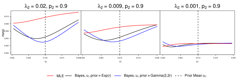
Figure 9: Asymptotic root mean-squared error (RMSE) of posterior mean for two Bayes estimators vs. MLE. Monte Carlo approximation to RMSE for posterior means, with standard error on the order of $10^{-6}$ for all $u_{1}$. Note an exponential prior puts prior mass near zero while the $\mathrm{gamma}(2,r_{1})$ prior puts vanishing prior mass as $u_{1}\to 0$. The $y$-axis represents the RMSE of the a given point estimator for certain data-generating values of $u_{1}$ and $u_{2}$. The panels of the graphs represent different true values of $u_{2}$, corresponding to $u_{2}=\lambda_{2}p_{2}$, while the $x$-axes represent a continuum of true values for $u_{1}$. The dashed vertical line represents the prior mean for $u_{1}$. Thus each panel of the graph shows how RMSE of each point estimator varies as $u_{1}$ increases from $4\times 10^{-6}$ to $1.9\times 10^{-2}$ given a certain value of $u_{2}$. The RMSE of the MLE, shown as the solid red line, slowly increases as $u_{1}$ increases as the variance of the MLE increases faster than the squared bias decreases. The Bayes estimators show decreasing RMSE as the prior mean for $u_{1}$ approaches the true $u_{1}$. Two conclusions can be drawn from the graphs: Both Bayes solutions dominate the MLE for reasonable values of $u_{1}$ and $u_{2}$. The exception is for small $u_{2}$ and when the prior for $u_{1}$ is several orders of magnitude too large. The second conclusion is that the Bayes estimator with gamma prior dominates the exponential-prior estimator when the prior mean for $u_{1}$ is moderately larger than the true $u_{1}$ and when the prior mean underestimates the true $u_{1}$.

Figure 9 shows that Bayes estimators yield gains over the MLE for minority groups. Within the class of Bayes estimators, estimators derived from models with priors that put too much support near zero (e.g. an exponential prior) can shrink too the posterior mean too strongly towards zero even when the prior mean over-estimates the true parameter. Given that the near-zero behavior is driven by the prior over $p_{1}$, limiting prior mass near $1$ for $p_{1}$ can yield point estimators with lower MSEs for a broad range of values for $u_{1}$.

D.3 DCT lemma

Lemma D.1.

Let $p_{\eta(\theta)}(X=k)$ be defined

$$\frac{1}{k!}\exp\left(\eta(\theta)k-e^{\eta(\theta)}\right),$$

where $\eta(\theta)$ is a univariate differentiable function of $\theta$, $\theta\in{}^{d}$. Let $g(\eta(\theta))=\int f(x)p_{\eta(\theta)}(x)d\mu(x)$ where $\mu$ is the counting measure on $[0,1,2,\dots]$. If we define the set $\theta\in\Theta_{f}$ as the set for which $\int\left|f(x)\right|p_{\eta(\theta)}(x)d\mu(x)<\infty$, then

$$\frac{\partial}{\partial\theta_{j}}g(\eta(\theta))=\int f(x)\frac{\partial}{\partial\theta_{j}}p_{\eta(\theta)}(x)d\mu(x)$$

Proof.

By the chain rule, the $\frac{\partial}{\partial\theta_{j}}g(\eta(\theta))=\frac{dg(\eta(\theta))}{d\eta(\theta)}\frac{\partial\eta(\theta)}{\partial\theta_{j}}$. By Theorem 2.4 in Keener (2010), $\frac{dg(\eta(\theta))}{d\eta(\theta)}$ exists and can be obtained via differentiating under the integral sign:

$$\frac{d}{d\eta(\theta)}g(\eta(\theta))=\int f(x)\frac{dp_{\eta(\theta)}(x)}{d\eta(\theta)}d\mu(x).$$

Using this result and the chain rule again yields

$$\frac{\partial}{\partial\theta_{j}}g(\eta(\theta)) =\frac{dg(\eta(\theta))}{d\eta(\theta)}\frac{\partial\eta(\theta)}{\partial\theta_{j}}$$ (40)

$$=\int f(x)\frac{dp_{\eta(\theta)}(x)}{d\eta(\theta)}\frac{\partial\eta(\theta)}{\partial\theta_{j}}d\mu(x)$$ (41)

$$=\int f(x)\frac{\partial}{\partial\theta_{j}}dp_{\eta(\theta)}(x)$$ (42)

∎

D.4 Lemmas and theorems in service of Fisher Info

Our local identifiability result is based on the following theorem that is referenced, though not proven, in Mukerjee and Sutradhar (2002). To our knowledge an explicit proof has not been given, though it follows directly from the proof of the Cramér-Rao lower bound in Rao (2002). This proof provides a slightly different route to showing local identifiability compared to that of Catchpole (1997). We give a proof below where we use the same notation as used in Rao (2002) for clarity’s sake.

Theorem D.2.

Suppose we have observations $X_{n}$ and let $\mathbf{x}\in{}^{N}$ be the collection of all observations, with the $n$-th element equal to $X_{n}$, where $\pi(\mathbf{x},\boldsymbol{\theta})$, parameterized by $\boldsymbol{\theta}\in{}^{d}$ with $i^{\textrm{th}}$ element $\theta_{i}$ is the joint density of the observations. Let $f_{1}(\mathbf{x}),\dots,f_{r}(\mathbf{x})$ be $r$ statistics for which $\mathbb{E}\left[f_{i}(\mathbf{x})\right]=g_{i}(\boldsymbol{\theta})$. Further, assume that $\frac{\partial}{\partial\theta_{j}}\int f_{i}(\mathbf{x})\pi(\mathbf{x},\boldsymbol{\theta})d\mathbf{x}=\int f_{i}(\mathbf{x})\frac{\partial}{\partial\theta_{j}}\pi(\mathbf{x},\boldsymbol{\theta})d\mathbf{x}=\frac{\partial g_{i}(\boldsymbol{\theta})}{\partial\theta_{j}}$. Let $\Delta$ be a matrix in ^r×d with elements $\Delta_{ij}=\frac{\partial g_{i}(\boldsymbol{\theta})}{\partial\theta_{j}}$. Let $\mathcal{I}$ be a matrix in ^d×d where the $(i,j)$-th element is defined as $\mathcal{I}_{ij}=\text{Cov}\left(\frac{\partial\log P(\mathbf{x},\boldsymbol{\theta})}{\partial\theta_{i}},\frac{\partial\log P(\mathbf{x},\boldsymbol{\theta})}{\partial\theta_{j}}\right)$. Let $\mathbf{V}$ be the matrix in ^r×r with $(i,j)$ elements $\mathbf{V}_{ij}=\text{Cov}\left(f_{i}(\mathbf{x}),f_{j}(\mathbf{x})\right)$. If $\mathbf{V}$ is positive definite, and $\Delta$ is full-rank, then the Fisher information matrix $\mathcal{I}$ is positive definite.

Proof.

Let $\mathbf{f}$ be the ordered collection of elements $f_{i}(\mathbf{x})$, and let $\nabla\log\pi(\mathbf{x},\boldsymbol{\theta})$ be the score vector. Then let the random vector $\rho=(\mathbf{f},\nabla\log\pi(\mathbf{x},\boldsymbol{\theta}))$. The covariance matrix associated with $\rho$, $\Sigma$, is a block matrix. Under $\pi(\mathbf{x},\boldsymbol{\theta})$, $\text{Cov}\left(f_{i},\frac{\partial\log\pi(\mathbf{x},\boldsymbol{\theta})}{\partial\theta_{j}}\right)=\frac{\partial g_{i}(\boldsymbol{\theta})}{\partial\theta_{j}}$, which is element $(i,j)$ of the matrix $\Delta$. The block covariance matrix for $\rho$ is:

$$\Sigma=\begin{bmatrix}\mathbf{V}&\Delta\\ \Delta^{T}&\mathcal{I}\end{bmatrix}$$

Suppose $\mathbf{V}$ is positive definite. We know $\mathcal{I}-\Delta^{T}\mathbf{V}^{-1}\Delta\succeq 0$, because $\Sigma$ is a covariance matrix which ensures it is positive semi definite. Furthermore, $\mathcal{I}\succeq\Delta^{T}\mathbf{V}^{-1}\Delta$. If $\Delta$ is full-rank then $\mathcal{I}\succ 0$. ∎

We need the following two lemmas to prove that the Fisher information is positive definite. First, the following lemma is stated in Tian (2004):

Lemma D.3.

Let $\mathbf{A}^{\dagger}$ be the Moore-Penrose inverse of a matrix $\mathbf{A}\in{}^{L\times M}$. Let $\mathbf{B}\in{}^{L\times T}$. The rank of a block matrix $[\mathbf{A}\,\,\mathbf{B}]$ is the rank of $\mathbf{A}$ plus the rank of $\mathbf{B}-\mathbf{A}\mathbf{A}^{\dagger}\mathbf{B}$.

Next, we will need this lemma later on:

Lemma D.4.

Suppose $\mathbf{W}\in{}^{I\times K}$ and $\mathbf{E}\in{}^{I\times J}$. Let $\mathbf{E}_{[:,j]}$ be an $I$-vector of the $j^{\textrm{th}}$ column of matrix $\mathbf{E}$, let $\mathbf{F}_{j}={\rm diag}(\mathbf{E}_{[:,j]})$.

1. $I\geq J+K$

2. ${\rm rank}\left(\mathbf{E}\right)=J$

3. ${\rm rank}\left(\mathbf{W}\right)=K$

4. $\forall i\in 1,\dots,I$ $\sum_{j=1}^{J}E_{ij}>0$

5. $\lambda_{j}>0\forall j\in 1,\dots,J$

6. ${\rm rank}\left(\begin{bmatrix}\mathbf{F}_{1}\mathbf{W}&\dots&\mathbf{F}_{J}\mathbf{W}&\mathbf{E}_{[:,1]}&\mathbf{E}_{[:,2]}&\dots&\mathbf{E}_{[:,J-1]}&\mathbf{E}_{[:,J]}\end{bmatrix}\right)>J+K$

Then the matrix

$$\begin{bmatrix}\left(\sum_{j}\lambda_{j}\mathbf{F}_{j}\right)\mathbf{W}&\mathbf{E}_{[:,1]}&\mathbf{E}_{[:,2]}&\dots&\mathbf{E}_{[:,J-1]}&\mathbf{E}_{[:,J]}\end{bmatrix}$$

is rank $J+K$.

Proof.

Given conditions (L.a) to (L.e) above , the matrix $\left(\sum_{j}\lambda_{j}\mathbf{F}_{j}\right)\mathbf{W}$ is rank $K$. Using lemma D.3 we proceed sequentially, showing first that

$$\text{rank}\left(\begin{bmatrix}\left(\sum_{j}\lambda_{j}\mathbf{F}_{j}\right)\mathbf{W}&\mathbf{E}_{[:,1]}\end{bmatrix}\right)=K+1$$

By D.3,

$$\text{rank}\left(\begin{bmatrix}\left(\sum_{j}\lambda_{j}\mathbf{F}_{j}\right)\mathbf{W}&\mathbf{E}_{[:,1]}\end{bmatrix}\right)= \text{rank}\left(\left(\sum_{j}\lambda_{j}\mathbf{F}_{j}\right)\mathbf{W}\right)$$

$$+\text{rank}\left(\mathbf{E}_{[:,1]}-\left(\sum_{j}\lambda_{j}\mathbf{F}_{j}\right)\mathbf{W}\left(\left(\sum_{j}\lambda_{j}\mathbf{F}_{j}\right)\mathbf{W}\right)^{\dagger}\mathbf{E}_{[:,1]}\right)$$

We can show that $\text{rank}\left(\mathbf{E}_{[:,1]}-\left(\sum_{j}\lambda_{j}\mathbf{F}_{j}\right)\mathbf{W}\left(\left(\sum_{j}\lambda_{j}\mathbf{F}_{j}\right)\mathbf{W}\right)^{\dagger}\mathbf{E}_{[:,1]}\right)=1$. We show by contradiction that given conditions on the coefficient matrix, no solution to the equation in $a_{k}$

$$\mathbf{E}_{[:,1]}=\sum_{k=1}^{K}a_{k}\left(\sum_{j=1}^{J}\lambda_{j}\mathbf{E}_{[:,j]}\odot\mathbf{W}_{k}\right)$$ (43)

can be found. This follows from examining the matrix of coefficients of the equation, shown here in block form:

$$\begin{bmatrix}\mathbf{E}_{[:,1]}&\lambda_{1}\mathbf{F}_{1}\mathbf{W}&\dots&\lambda_{J}\mathbf{F}_{J}\mathbf{W}\end{bmatrix}$$ (44)

Given condition (L.e), $\lambda_{j}>0$ for all $j$, for a fixed set of parameters $\lambda_{j}$ the matrix in eq. 44 has the same column space as

$$\begin{bmatrix}\mathbf{E}_{[:,1]}&\mathbf{F}_{1}\mathbf{W}&\dots&\mathbf{F}_{J}\mathbf{W}\end{bmatrix}$$ (45)

Given condition (L.f), matrix 45 has rank greater than $K$, so the system of equations in 43 will not have a solution in $a_{k},k\in[1,\dots,K]$. Thus the rank of matrix

$$\mathbf{E}_{[:,1]}-\left(\sum_{j}\lambda_{j}\mathbf{F}_{j}\right)\mathbf{W}\left(\left(\sum_{j}\lambda_{j}\mathbf{F}_{j}\right)\mathbf{W}\right)^{\dagger}\mathbf{E}_{[:,1]}$$ (46)

is $1$ so the rank of .

$$\begin{bmatrix}\left(\sum_{j}\lambda_{j}\mathbf{F}_{j}\right)\mathbf{W}&\mathbf{E}_{[:,1]}\end{bmatrix}$$

is $K+1$.

Now for the induction step: Suppose that

$$\begin{bmatrix}\left(\sum_{j}\lambda_{j}\mathbf{F}_{j}\right)\mathbf{W}&\mathbf{E}_{[:,1:M]}\end{bmatrix}$$

is rank $M+K$ and suppose we want to determine the rank of

$$\begin{bmatrix}\left(\sum_{j}\lambda_{j}\mathbf{F}_{j}\right)\mathbf{W}&\mathbf{E}_{[:,1:M]}&\mathbf{E}_{[:,M+1]}\end{bmatrix}.$$

By lemma D.3, the rank of the above matrix is

$$\text{rank}\begin{bmatrix}\left(\sum_{j}\lambda_{j}\mathbf{F}_{j}\right)\mathbf{W}&\mathbf{E}_{[:,1:M]}\end{bmatrix}$$ (47)

$$+\text{rank}\left(\mathbf{E}_{[:,M+1]}-\begin{bmatrix}\left(\sum_{j}\lambda_{j}\mathbf{F}_{j}\right)\mathbf{W}&\mathbf{E}_{[:,1:M]}\end{bmatrix}\begin{bmatrix}\left(\sum_{j}\lambda_{j}\mathbf{F}_{j}\right)\mathbf{W}&\mathbf{E}_{[:,1:M]}\end{bmatrix}^{\dagger}\mathbf{E}_{[:,M+1]}\right)$$ (48)

By the induction hypothesis, we know that eq. 47 equals $K+M$ and we look to see whether eq. 48 equals 1 by determining whether the system of equations below:

$$\mathbf{E}_{[:,M+1]}=\sum_{k=1}^{K}a_{k}\left(\sum_{j=1}^{J}\lambda_{j}\mathbf{E}_{j}\odot\mathbf{W}_{k}\right)+\sum_{m=1}^{M}d_{m}\mathbf{E}_{[:,m]}$$ (49)

has a solution in the variables $a_{k},k\in[1,\dots,K]$, $d_{m},m\in[1,\dots,M],M<J$. Then for a fixed $\{\lambda_{j},j\in[1,\dots,J]\}$ the coefficient matrix for the system of equations in eq. 49 has the same column space as

$$\begin{bmatrix}\mathbf{E}_{[:,M+1]}&\mathbf{F}_{1}\mathbf{W}&\dots&\mathbf{F}_{J}\mathbf{W}&\mathbf{E}_{[:,1:M]}\end{bmatrix}$$ (50)

By condition (L.f), the rank of matrix (50) is greater than $M+K$, which precludes $\mathbf{E}_{[:,M+1]}$ from lying in the column space of

$$\begin{bmatrix}\left(\sum_{j}\lambda_{j}\mathbf{F}_{j}\right)\mathbf{W}&\mathbf{E}_{[:,1:M]}\end{bmatrix}$$

. Thus the line (48) is equal to $1$ and summing with line (47) shows that the rank of

$$\begin{bmatrix}\left(\sum_{j}\lambda_{j}\mathbf{F}_{j}\right)\mathbf{W}&\mathbf{E}_{[:,1:M]}&\mathbf{E}_{[:,M+1]}\end{bmatrix}$$

is $M+1+K$. Therefore by induction,

$$\begin{bmatrix}\left(\sum_{j}\lambda_{j}\mathbf{F}_{j}\right)\mathbf{W}&\mathbf{E}_{[:,1]}&\mathbf{E}_{[:,2]}&\dots&\mathbf{E}_{[:,J-1]}&\mathbf{E}_{[:,J]}\end{bmatrix}$$

is rank $J+K$. ∎

Appendix E Full model local identifiability proof

Proof.

In order to draw on the results of D.2, we must ensure $\frac{\partial}{\partial\theta_{j}}\int f_{i}\pi(\mathbf{x},\theta)d\nu=\int f_{i}\frac{\partial}{\partial\theta_{j}}\pi(\mathbf{x},\theta)d\nu$ holds for model (10). This condition does indeed hold by lemma D.1 because our observational density is an exponential family density. Now we look for moment estimators, $\mathbf{f}=(f_{1},\dots,f_{r})$ with full-rank $\Delta$ and positive definite covariance matrices. As shown in section B, conditionally on unknown parameters, known covariates $\mathbf{z}_{i}$ and population counts $\mathbf{e}_{i}$, $X_{ij}$ is independent of $M_{i}$ for all $i$ and $j$. Let $\mathbf{x}_{j}=(X_{1j},X_{2j},\dots,X_{Ij})$, and set

$$\mathbf{f}=(\mathbf{x}_{1},\mathbf{x}_{2},\dots,\mathbf{x}_{J},M_{1},M_{2},\dots,M_{I}).$$

From the independence of the elements of the vector $(X_{i1},X_{i2},\dots,X_{iJ},,M_{i})^{T}$, and the conditional independence between observations $i$, $\text{Cov}(\mathbf{f})$ is diagonal, and is positive definite because conditions (S.d) to (S.f) are assumed to hold. The final condition for theorem D.2 to hold, which establishes a lower bound on the positive definiteness of the Fisher information matrix is to ensure that $\Delta$ has full column-rank. To that end, let us calculate $\Delta$, beginning with $\mathbb{E}\left[\mathbf{f}\right]$: The expected value of $\mathbf{f}$ is the vector:

$$\begin{bmatrix}E_{11}p_{11}e^{\mathbf{z}_{1}^{T}\boldsymbol{\beta}}\lambda_{1}\\ E_{21}p_{21}e^{\mathbf{z}_{2}^{T}\boldsymbol{\beta}}\lambda_{1}\\ \vdots\\ E_{I1}p_{I1}e^{\mathbf{z}_{I}^{T}\boldsymbol{\beta}}\lambda_{1}\\ E_{12}p_{12}e^{\mathbf{z}_{1}^{T}\boldsymbol{\beta}}\lambda_{2}\\ E_{22}p_{22}e^{\mathbf{z}_{2}^{T}\boldsymbol{\beta}}\lambda_{2}\\ \vdots\\ E_{I2}p_{I2}e^{\mathbf{z}_{I}^{T}\boldsymbol{\beta}}\lambda_{2}\\ \vdots\\ E_{1J}p_{1J}e^{\mathbf{z}_{1}^{T}\boldsymbol{\beta}}\lambda_{J}\\ E_{2J}p_{2J}e^{\mathbf{z}_{2}^{T}\boldsymbol{\beta}}\lambda_{J}\\ \vdots\\ E_{IJ}p_{IJ}e^{\mathbf{z}_{I}^{T}\boldsymbol{\beta}}\lambda_{J}\\ \sum_{j}E_{1j}(1-p_{1j})e^{\mathbf{z}_{1}^{T}\boldsymbol{\beta}}\lambda_{j}\\ \vdots\\ \sum_{j}E_{Ij}(1-p_{Ij})e^{\mathbf{z}_{I}^{T}\boldsymbol{\beta}}\lambda_{j}\end{bmatrix}$$

For efficiency of notation, let $c_{ij}=p_{ij}\lambda_{j}$ $p^{\prime}_{ij}=p_{ij}(1-p_{ij})$, and $q_{ij}=(1-p_{ij})$ Let $\mathbf{H}$ by the $(J+1)I\times 2K$ matrix of partial derivatives of $\mathbb{E}\left[\mathbf{f}\right]$ with respect to the vector $(\boldsymbol{\beta},\boldsymbol{\gamma})$:

$$\mathbf{H}=\begin{bmatrix}\mathbf{z}_{1}^{T}E_{11}c_{11}e^{\mathbf{z}_{1}^{T}\boldsymbol{\beta}}&\mathbf{z}_{1}^{T}E_{11}p^{\prime}_{11}\lambda_{1}e^{\mathbf{z}_{1}^{T}\boldsymbol{\beta}}\\ \mathbf{z}_{2}^{T}E_{21}c_{21}e^{\mathbf{z}_{2}^{T}\boldsymbol{\beta}}&\mathbf{z}_{2}^{T}E_{21}p^{\prime}_{21}\lambda_{1}e^{\mathbf{z}_{2}^{T}\boldsymbol{\beta}}\\ \vdots&\vdots\\ \mathbf{z}_{I}^{T}E_{I1}c_{I1}e^{\mathbf{z}_{I}^{T}\boldsymbol{\beta}}&\mathbf{z}_{I}^{T}E_{I1}p^{\prime}_{I1}\lambda_{1}e^{\mathbf{z}_{I}^{T}\boldsymbol{\beta}}\\ \mathbf{z}_{1}^{T}E_{12}c_{12}e^{\mathbf{z}_{1}^{T}\boldsymbol{\beta}}&\mathbf{z}_{1}^{T}E_{12}p^{\prime}_{12}\lambda_{2}e^{\mathbf{z}_{1}^{T}\boldsymbol{\beta}}\\ \mathbf{z}_{2}^{T}E_{22}c_{22}e^{\mathbf{z}_{2}^{T}\boldsymbol{\beta}}&\mathbf{z}_{2}^{T}E_{21}p^{\prime}_{22}\lambda_{2}e^{\mathbf{z}_{2}^{T}\boldsymbol{\beta}}\\ \vdots&\vdots\\ \mathbf{z}_{I}^{T}E_{I2}c_{I2}e^{\mathbf{z}_{I}^{T}\boldsymbol{\beta}}&\mathbf{z}_{I}^{T}E_{I2}p^{\prime}_{I2}\lambda_{2}e^{\mathbf{z}_{I}^{T}\boldsymbol{\beta}}\\ \vdots&\vdots\\ \mathbf{z}_{1}^{T}E_{1J}c_{1J}e^{\mathbf{z}_{1}^{T}\boldsymbol{\beta}}&\mathbf{z}_{1}^{T}E_{1J}p^{\prime}_{1J}\lambda_{J}e^{\mathbf{z}_{1}^{T}\boldsymbol{\beta}}\\ \mathbf{z}_{2}^{T}E_{2J}c_{2J}e^{\mathbf{z}_{2}^{T}\boldsymbol{\beta}}&\mathbf{z}_{2}^{T}E_{2J}p^{\prime}_{2J}\lambda_{J}e^{\mathbf{z}_{2}^{T}\boldsymbol{\beta}}\\ \vdots&\vdots\\ \mathbf{z}_{I}^{T}E_{IJ}c_{IJ}e^{\mathbf{z}_{I}^{T}\boldsymbol{\beta}}&\mathbf{z}_{I}^{T}E_{IJ}p^{\prime}_{IJ}\lambda_{J}e^{\mathbf{z}_{I}^{T}\boldsymbol{\beta}}\\ \mathbf{z}_{1}^{T}e^{\mathbf{z}_{1}^{T}\boldsymbol{\beta}}\sum_{j}E_{1j}q_{1j}\lambda_{j}&-\mathbf{z}_{1}^{T}e^{\mathbf{z}_{1}^{T}\boldsymbol{\beta}}\sum_{j}E_{1j}p^{\prime}_{1j}\lambda_{j}\\ \vdots&\vdots\\ \mathbf{z}_{I}^{T}e^{\mathbf{z}_{I}^{T}\boldsymbol{\beta}}\sum_{j}E_{Ij}q_{Ij}\lambda_{j}&-\mathbf{z}_{I}^{T}e^{\mathbf{z}_{I}^{T}\boldsymbol{\beta}}\sum_{j}E_{Ij}p^{\prime}_{Ij}\lambda_{j}\end{bmatrix}$$

Let $\mathbf{T}$ be the $(J+1)I\times 2J$ matrix of partial derivatives with respect to $(\lambda_{1},\lambda_{2},\dots,\lambda_{J},\eta_{1},\eta_{2},\dots,\eta_{J})$,

$$\mathbf{T}=\begin{bmatrix}E_{11}p_{11}e^{\mathbf{z}_{1}^{T}\boldsymbol{\beta}}&0&\dots&0&E_{11}p^{\prime}_{11}\lambda_{1}e^{\mathbf{z}_{1}^{T}\boldsymbol{\beta}}&0&\dots&0\\ E_{21}p_{21}e^{\mathbf{z}_{2}^{T}\boldsymbol{\beta}}&0&\dots&0&E_{21}p^{\prime}_{21}\lambda_{1}e^{\mathbf{z}_{2}^{T}\boldsymbol{\beta}}&0&\dots&0\\ \vdots&\vdots&\vdots&\vdots&\vdots&\vdots&\vdots&\vdots\\ E_{I1}p_{I1}e^{\mathbf{z}_{I}^{T}\boldsymbol{\beta}}&0&\dots&0&E_{I1}p^{\prime}_{I1}\lambda_{1}e^{\mathbf{z}_{I}^{T}\boldsymbol{\beta}}&0&\dots&0\\ 0&E_{12}p_{12}e^{\mathbf{z}_{1}^{T}\boldsymbol{\beta}}&\dots&0&0&E_{12}p^{\prime}_{12}\lambda_{2}e^{\mathbf{z}_{1}^{T}\boldsymbol{\beta}}&\dots&0\\ 0&E_{22}p_{22}e^{\mathbf{z}_{2}^{T}\boldsymbol{\beta}}&\dots&0&0&E_{22}p^{\prime}_{22}\lambda_{2}e^{\mathbf{z}_{2}^{T}\boldsymbol{\beta}}&\dots&0\\ \vdots&\vdots&\vdots&\vdots&\vdots&\vdots&\vdots&\vdots\\ 0&E_{I2}p_{I2}e^{\mathbf{z}_{I}^{T}\boldsymbol{\beta}}&\dots&0&0&E_{I2}p^{\prime}_{I2}\lambda_{2}e^{\mathbf{z}_{I}^{T}\boldsymbol{\beta}}&\dots&0\\ \vdots&\vdots&\ddots&\vdots&\vdots&\vdots&\ddots&\vdots\\ 0&0&\dots&E_{1J}p_{1J}e^{\mathbf{z}_{1}^{T}\boldsymbol{\beta}}&0&0&\dots&E_{1J}p^{\prime}_{1J}\lambda_{J}e^{\mathbf{z}_{1}^{T}\boldsymbol{\beta}}\\ 0&0&\dots&E_{2J}p_{2J}e^{\mathbf{z}_{2}^{T}\boldsymbol{\beta}}&0&0&\dots&E_{2J}p^{\prime}_{2J}\lambda_{J}e^{\mathbf{z}_{2}^{T}\boldsymbol{\beta}}\\ \vdots&\vdots&\vdots&\vdots&\vdots&\vdots&\vdots&\vdots\\ 0&0&\dots&E_{IJ}p_{IJ}e^{\mathbf{z}_{I}^{T}\boldsymbol{\beta}}&0&0&\dots&E_{IJ}p^{\prime}_{IJ}\lambda_{J}e^{\mathbf{z}_{I}^{T}\boldsymbol{\beta}}\\ E_{11}q_{11}e^{\mathbf{z}_{1}^{T}\boldsymbol{\beta}}&E_{12}q_{12}e^{\mathbf{z}_{1}^{T}\boldsymbol{\beta}}&\dots&E_{1J}q_{1J}e^{\mathbf{z}_{1}^{T}\boldsymbol{\beta}}&-E_{11}p^{\prime}_{11}\lambda_{1}e^{\mathbf{z}_{1}^{T}\boldsymbol{\beta}}&-E_{12}p^{\prime}_{12}\lambda_{2}e^{\mathbf{z}_{1}^{T}\boldsymbol{\beta}}&\dots&-E_{1J}p^{\prime}_{1J}\lambda_{J}e^{\mathbf{z}_{1}^{T}\boldsymbol{\beta}}\\ \vdots&\vdots&\ddots&\vdots&\vdots&\vdots&\ddots&\vdots\\ E_{I1}q_{I1}e^{\mathbf{z}_{I}^{T}\boldsymbol{\beta}}&E_{I2}q_{I2}e^{\mathbf{z}_{I}^{T}\boldsymbol{\beta}}&\dots&E_{IJ}q_{IJ}e^{\mathbf{z}_{I}^{T}\boldsymbol{\beta}}&-E_{I1}p^{\prime}_{I1}\lambda_{1}e^{\mathbf{z}_{I}^{T}\boldsymbol{\beta}}&-E_{I2}p^{\prime}_{I2}\lambda_{2}e^{\mathbf{z}_{I}^{T}\boldsymbol{\beta}}&\dots&-E_{IJ}p^{\prime}_{IJ}\lambda_{J}e^{\mathbf{z}_{I}^{T}\boldsymbol{\beta}}\\ \end{bmatrix}$$

Then

$$\Delta =\begin{bmatrix}\mathbf{T}&\mathbf{H}\end{bmatrix}$$

Let the matrix $\mathbf{R}_{i,j}(m)$ be the elementary row-addition matrix. When a matrix $\mathbf{A}\in{}^{M\times N}$ is left-multiplied by $\mathbf{R}_{ij}(m)$, $\tilde{\mathbf{A}}=\mathbf{E}_{ij}(m)\mathbf{A}$, all rows of $\tilde{\mathbf{A}}$ equal that of $\mathbf{A}$ excepting $\tilde{\mathbf{A}}$’s $i$-th row, which is $\tilde{\mathbf{A}}_{[i,:]}=\mathbf{A}_{[i,:]}+m\mathbf{A}_{[j,:]}$. Let $\tilde{\mathbf{H}}$ and $\tilde{\mathbf{T}}$ be the result of left-multiplying $\mathbf{H}$ and $\mathbf{T}$ by the same product of elementary row-addition matrices, namely:

$$\prod_{i=1}^{I}\prod_{j=1}^{J}\mathbf{R}_{JI+j,(j-1)I+i}(1)$$

Then let $\tilde{\Delta}$ be the matrix $\Delta$ after applying the product of elementary row-addition matrices:

$$\tilde{\Delta} =\prod_{i=1}^{I}\prod_{j=1}^{J}\mathbf{R}_{JI+j,(j-1)I+i}(1)\begin{bmatrix}\mathbf{T}&\mathbf{H}\end{bmatrix}$$

$$=\begin{bmatrix}\prod_{i=1}^{I}\prod_{j=1}^{J}\mathbf{R}_{JI+j,(j-1)I+i}(1)\mathbf{T}&\prod_{i=1}^{I}\prod_{j=1}^{J}\mathbf{R}_{JI+j,(j-1)I+i}(1)\mathbf{H}\end{bmatrix}$$

$$=\begin{bmatrix}\tilde{\mathbf{T}}&\tilde{\mathbf{H}}\end{bmatrix}$$

where

$$\tilde{\mathbf{H}}=\begin{bmatrix}\mathbf{z}_{1}^{T}E_{11}c_{11}e^{\mathbf{z}_{1}^{T}\boldsymbol{\beta}}&\mathbf{z}_{1}^{T}E_{11}p^{\prime}_{11}\lambda_{1}e^{\mathbf{z}_{1}^{T}\boldsymbol{\beta}}\\ \mathbf{z}_{2}^{T}E_{21}c_{21}e^{\mathbf{z}_{2}^{T}\boldsymbol{\beta}}&\mathbf{z}_{2}^{T}E_{21}p^{\prime}_{21}\lambda_{1}e^{\mathbf{z}_{2}^{T}\boldsymbol{\beta}}\\ \vdots&\vdots\\ \mathbf{z}_{I}^{T}E_{I1}c_{I1}e^{\mathbf{z}_{I}^{T}\boldsymbol{\beta}}&\mathbf{z}_{I}^{T}E_{I1}p^{\prime}_{I1}\lambda_{1}e^{\mathbf{z}_{I}^{T}\boldsymbol{\beta}}\\ \mathbf{z}_{1}^{T}E_{12}c_{12}e^{\mathbf{z}_{1}^{T}\boldsymbol{\beta}}&\mathbf{z}_{1}^{T}E_{12}p^{\prime}_{12}\lambda_{2}e^{\mathbf{z}_{1}^{T}\boldsymbol{\beta}}\\ \mathbf{z}_{2}^{T}E_{22}c_{22}e^{\mathbf{z}_{2}^{T}\boldsymbol{\beta}}&\mathbf{z}_{2}^{T}E_{21}p^{\prime}_{22}\lambda_{2}e^{\mathbf{z}_{2}^{T}\boldsymbol{\beta}}\\ \vdots&\vdots\\ \mathbf{z}_{I}^{T}E_{I2}c_{I2}e^{\mathbf{z}_{I}^{T}\boldsymbol{\beta}}&\mathbf{z}_{I}^{T}E_{I2}p^{\prime}_{I2}\lambda_{2}e^{\mathbf{z}_{I}^{T}\boldsymbol{\beta}}\\ \vdots&\vdots\\ \mathbf{z}_{1}^{T}E_{1J}c_{1J}e^{\mathbf{z}_{1}^{T}\boldsymbol{\beta}}&\mathbf{z}_{1}^{T}E_{1J}p^{\prime}_{1J}\lambda_{J}e^{\mathbf{z}_{1}^{T}\boldsymbol{\beta}}\\ \mathbf{z}_{2}^{T}E_{2J}c_{2J}e^{\mathbf{z}_{2}^{T}\boldsymbol{\beta}}&\mathbf{z}_{2}^{T}E_{2J}p^{\prime}_{2J}\lambda_{J}e^{\mathbf{z}_{2}^{T}\boldsymbol{\beta}}\\ \vdots&\vdots\\ \mathbf{z}_{I}^{T}E_{IJ}c_{IJ}e^{\mathbf{z}_{I}^{T}\boldsymbol{\beta}}&\mathbf{z}_{I}^{T}E_{IJ}p^{\prime}_{IJ}\lambda_{J}e^{\mathbf{z}_{I}^{T}\boldsymbol{\beta}}\\ \mathbf{z}_{1}^{T}e^{\mathbf{z}_{1}^{T}\boldsymbol{\beta}}\sum_{j}E_{1j}\lambda_{j}&0_{1\times K}\\ \vdots&\vdots\\ \mathbf{z}_{I}^{T}e^{\mathbf{z}_{I}^{T}\boldsymbol{\beta}}\sum_{j}E_{Ij}\lambda_{j}&0_{1\times K}\end{bmatrix},$$

and

$$\tilde{\mathbf{T}}=\begin{bmatrix}E_{11}p_{11}e^{\mathbf{z}_{1}^{T}\boldsymbol{\beta}}&0&\dots&0&E_{11}p^{\prime}_{11}\lambda_{1}e^{\mathbf{z}_{1}^{T}\boldsymbol{\beta}}&0&\dots&0\\ E_{21}p_{21}e^{\mathbf{z}_{2}^{T}\boldsymbol{\beta}}&0&\dots&0&E_{21}p^{\prime}_{21}\lambda_{1}e^{\mathbf{z}_{2}^{T}\boldsymbol{\beta}}&0&\dots&0\\ \vdots&\vdots&\vdots&\vdots&\vdots&\vdots&\vdots&\vdots\\ E_{I1}p_{I1}e^{\mathbf{z}_{I}^{T}\boldsymbol{\beta}}&0&\dots&0&E_{I1}p^{\prime}_{I1}\lambda_{1}e^{\mathbf{z}_{I}^{T}\boldsymbol{\beta}}&0&\dots&0\\ 0&E_{12}p_{12}e^{\mathbf{z}_{1}^{T}\boldsymbol{\beta}}&\dots&0&0&E_{12}p^{\prime}_{12}\lambda_{2}e^{\mathbf{z}_{1}^{T}\boldsymbol{\beta}}&\dots&0\\ 0&E_{22}p_{22}e^{\mathbf{z}_{2}^{T}\boldsymbol{\beta}}&\dots&0&0&E_{22}p^{\prime}_{22}\lambda_{2}e^{\mathbf{z}_{2}^{T}\boldsymbol{\beta}}&\dots&0\\ \vdots&\vdots&\vdots&\vdots&\vdots&\vdots&\vdots&\vdots\\ 0&E_{I2}p_{I2}e^{\mathbf{z}_{I}^{T}\boldsymbol{\beta}}&\dots&0&0&E_{I2}p^{\prime}_{I2}\lambda_{2}e^{\mathbf{z}_{I}^{T}\boldsymbol{\beta}}&\dots&0\\ \vdots&\vdots&\ddots&\vdots&\vdots&\vdots&\ddots&\vdots\\ 0&0&\dots&E_{1J}p_{1J}e^{\mathbf{z}_{1}^{T}\boldsymbol{\beta}}&0&0&\dots&E_{1J}p^{\prime}_{1J}\lambda_{J}e^{\mathbf{z}_{1}^{T}\boldsymbol{\beta}}\\ 0&0&\dots&E_{2J}p_{2J}e^{\mathbf{z}_{2}^{T}\boldsymbol{\beta}}&0&0&\dots&E_{2J}p^{\prime}_{2J}\lambda_{J}e^{\mathbf{z}_{2}^{T}\boldsymbol{\beta}}\\ \vdots&\vdots&\vdots&\vdots&\vdots&\vdots&\vdots&\vdots\\ 0&0&\dots&E_{IJ}p_{IJ}e^{\mathbf{z}_{I}^{T}\boldsymbol{\beta}}&0&0&\dots&E_{IJ}p^{\prime}_{IJ}\lambda_{J}e^{\mathbf{z}_{I}^{T}\boldsymbol{\beta}}\\ E_{11}e^{\mathbf{z}_{1}^{T}\boldsymbol{\beta}}&E_{12}e^{\mathbf{z}_{1}^{T}\boldsymbol{\beta}}&\dots&E_{1J}e^{\mathbf{z}_{1}^{T}\boldsymbol{\beta}}&0&0&\dots&0\\ \vdots&\vdots&\ddots&\vdots&\vdots&\vdots&\ddots&\vdots\\ E_{I1}e^{\mathbf{z}_{I}^{T}\boldsymbol{\beta}}&E_{I2}e^{\mathbf{z}_{I}^{T}\boldsymbol{\beta}}&\dots&E_{IJ}e^{\mathbf{z}_{I}^{T}\boldsymbol{\beta}}&0&0&\dots&0\\ \end{bmatrix}.$$

We can represent $\tilde{\mathbf{T}}$ and $\tilde{\mathbf{H}}$ as block matrices. We let $\mathbf{E}$ be the $I\times J$ matrix with $(i,j)^{\text{th}}$ elements $E_{ij}$, and we similarly define the matrix $\mathbf{C}$ to be in ^I×J with its $i,j$ element equal to $c_{ij}$. Furthermore, let $\mathbf{p}^{\prime}_{ij}=p^{\prime}_{ij}$. Let the matrix $\boldsymbol{\omega}$ be the diagonal matrix in ^I×I with $i,j$ elements $e^{\mathbf{z}_{i}^{T}\boldsymbol{\beta}}\mathbbm{1}(i=j)$. Let $\mathbf{E}_{[:,j]}\odot\mathbf{C}_{[:,j]}$ be the element-wise multiplication between the two matrices $\mathbf{E}_{[:,j]}$ and $\mathbf{C}_{[:,j]}$. Let $\mathbf{Z}\in{}^{I\times K}$ with rows $\mathbf{Z}_{[i,:]}=\mathbf{z}_{i}^{T}$. Let $\mathbf{1}$ be the $I$-dimensional vector with each element equal to 1 and let

$$\mathbf{D}_{j} =\text{diag}(\mathbf{E}_{[:,j]}\odot\mathbf{C}_{[:,j]})$$

$$\mathbf{D}^{\prime}_{j} =\text{diag}(\mathbf{E}_{[:,j]}\odot\mathbf{p}^{\prime}_{[:,j]})$$

$$\mathbf{F}_{j} =\text{diag}(\mathbf{E}_{[:,j]}).$$

Let $\boldsymbol{\Omega}$ be the block matrix:

$$\boldsymbol{\Omega}=\begin{bmatrix}\boldsymbol{\omega}&0_{I\times I}&\dots&0_{I\times I}&0_{I\times I}&0_{I\times I}\\ 0_{I\times I}&\boldsymbol{\omega}&\dots&0_{I\times I}&0_{I\times I}&0_{I\times I}\\ \vdots&\vdots&\ddots&\vdots&\vdots&\vdots\\ 0_{I\times I}&0_{I\times I}&\dots&\boldsymbol{\omega}&0_{I\times I}&0_{I\times I}\\ 0_{I\times I}&0_{I\times I}&\dots&0_{I\times I}&\boldsymbol{\omega}&0_{I\times I}\\ 0_{I\times I}&0_{I\times I}&\dots&0_{I\times I}&0_{I\times I}&\boldsymbol{\omega}\end{bmatrix}$$ (51)

Then we can write $\tilde{\mathbf{H}}$ as

$$\boldsymbol{\Omega}\begin{bmatrix}\mathbf{D}_{1}\mathbf{Z}&\mathbf{D}_{1}^{\prime}\mathbf{Z}\lambda_{1}\\ \mathbf{D}_{2}\mathbf{Z}&\mathbf{D}_{2}^{\prime}\mathbf{Z}\lambda_{2}\\ \vdots&\vdots\\ \mathbf{D}_{J-1}\mathbf{Z}&\mathbf{D}_{J-1}^{\prime}\mathbf{Z}\lambda_{J-1}\\ \mathbf{D}_{J}\mathbf{Z}&\mathbf{D}_{J}^{\prime}\mathbf{Z}\lambda_{J}\\ \left(\sum_{j}\lambda_{j}\mathbf{F}_{j}\right)\mathbf{Z}&0_{I\times K}\\ \end{bmatrix}$$ (52)

and $\tilde{\mathbf{T}}$ as

$$\boldsymbol{\Omega}\begin{bmatrix}\mathbf{D}_{1}\mathbf{1}&0_{I\times 1}&\dots&0_{I\times 1}&0_{I\times 1}&\lambda_{1}\mathbf{D}_{1}^{\prime}\mathbf{1}&0_{I\times 1}&\dots&0_{I\times 1}&0_{I\times 1}\\ 0_{I\times 1}&\mathbf{D}_{2}\mathbf{1}&\dots&0_{I\times 1}&0_{I\times 1}&0_{I\times 1}&\lambda_{2}\mathbf{D}^{\prime}_{2}\mathbf{1}&\dots&0_{I\times 1}&0_{I\times 1}\\ \vdots&\vdots&\ddots&\vdots&\vdots&\vdots&\vdots&\ddots&\vdots&\vdots\\ 0_{I\times 1}&0_{I\times 1}&\dots&\mathbf{D}_{J-1}\mathbf{1}&0_{I\times 1}&0_{I\times 1}&0_{I\times 1}&\dots&\lambda_{J-1}\mathbf{D}^{\prime}_{J-1}\mathbf{1}&0_{I\times 1}\\ 0_{I\times 1}&0_{I\times 1}&\dots&0_{I\times 1}&\mathbf{D}_{J}\mathbf{1}&0_{I\times 1}&0_{I\times 1}&\dots&0_{I\times 1}&\lambda_{J}\mathbf{D}^{\prime}_{J}\mathbf{1}\\ \mathbf{E}_{[:,1]}&\mathbf{E}_{[:,2]}&\dots&\mathbf{E}_{[:,J-1]}&\mathbf{E}_{[:,J]}&0_{I\times 1}&0_{I\times 1}&\dots&0_{I\times 1}&0_{I\times 1}\end{bmatrix}$$ (53)

Rearranging the columns of $\tilde{\Delta}$ to form $\tilde{\Delta}^{\prime}$ does not change the rank of the matrix, and clarifies the conditions needed for the matrix to be full-rank:

$$\tilde{\Delta}^{\prime}=\boldsymbol{\Omega}\setcounter{MaxMatrixCols}{12}\begin{bmatrix}\mathbf{D}_{1}\mathbf{Z}&\mathbf{D}_{1}\mathbf{1}&0_{I\times 1}&\dots&0_{I\times 1}&0_{I\times 1}&\lambda_{1}\mathbf{D}_{1}^{\prime}\mathbf{Z}&0_{I\times 1}&\lambda_{1}\mathbf{D}_{1}^{\prime}\mathbf{1}&0_{I\times 1}&\dots&0_{I\times 1}\\ \mathbf{D}_{2}\mathbf{Z}&0_{I\times 1}&\mathbf{D}_{2}\mathbf{1}&\dots&0_{I\times 1}&0_{I\times 1}&\lambda_{2}\mathbf{D}_{2}^{\prime}\mathbf{Z}&0_{I\times 1}&0_{I\times 1}&\lambda_{2}\mathbf{D}^{\prime}_{2}\mathbf{1}&\dots&0_{I\times 1}\\ \vdots&\vdots&\vdots&\ddots&\vdots&\vdots&\vdots&\vdots&\vdots&\vdots&\ddots&\vdots\\ \mathbf{D}_{J-1}\mathbf{Z}&0_{I\times 1}&0_{I\times 1}&\dots&\mathbf{D}_{J-1}\mathbf{1}&0_{I\times 1}&\lambda_{J-1}\mathbf{D}^{\prime}_{J-1}\mathbf{Z}&0_{I\times 1}&0_{I\times 1}&0_{I\times 1}&\dots&\lambda_{J-1}\mathbf{D}_{J-1}^{\prime}\mathbf{1}\\ \mathbf{D}_{J}\mathbf{Z}&0_{I\times 1}&0_{I\times 1}&\dots&0_{I\times 1}&\mathbf{D}_{J}\mathbf{1}&\lambda_{J}\mathbf{D}^{\prime}_{J}\mathbf{Z}&\lambda_{J}\mathbf{D}_{J}^{\prime}\mathbf{1}&0_{I\times 1}&0_{I\times 1}&\dots&0_{I\times 1}\\ \left(\sum_{j}\lambda_{j}\mathbf{F}_{j}\right)\mathbf{Z}&\mathbf{E}_{[:,1]}&\mathbf{E}_{[:,2]}&\dots&\mathbf{E}_{[:,J-1]}&\mathbf{E}_{[:,J]}&0_{I\times K}&0_{I\times 1}&0_{I\times 1}&0_{I\times 1}&\dots&0_{I\times 1}\end{bmatrix}$$ (54)

is $\in{}^{\left(I(J+1)\right)\times\left(2K+2J\right)}$. The first matrix $\boldsymbol{\Omega}$ is a $I(J+1)\times I(J+1)$ block diagonal matrix of diagonal matrices and by condition (S.f) is rank $I(J+1)$. Then the product in equation (54) is rank $2K+2J$ if the second matrix above is rank $2K+2J$ by Sylvester’s rank inequality. The second matrix above is rank $2K+2J$ if the following three sub-blocks are full column rank:

$$\mathbf{L}_{1}=\begin{bmatrix}\lambda_{1}\mathbf{D}_{1}^{\prime}\mathbf{1}&0_{I\times 1}&\dots&0_{I\times 1}\\ 0_{I\times 1}&\lambda_{2}\mathbf{D}^{\prime}_{2}\mathbf{1}&\dots&0_{I\times 1}\\ \vdots&\vdots&\ddots&\vdots\\ 0_{I\times 1}&0_{I\times 1}&\dots&\lambda_{J-1}\mathbf{D}^{\prime}_{J-1}\mathbf{1}\end{bmatrix}$$ (55)

and

$$\mathbf{L}_{2}=\begin{bmatrix}\left(\sum_{j}\lambda_{j}\mathbf{F}_{j}\right)\mathbf{Z}&\mathbf{E}_{[:,1]}&\mathbf{E}_{[:,2]}&\dots&\mathbf{E}_{[:,J-1]}&\mathbf{E}_{[:,J]}\end{bmatrix}$$ (56)

and

$$\mathbf{L}_{3}=\begin{bmatrix}\lambda_{J}\mathbf{D}^{\prime}_{J}\mathbf{Z}&\lambda_{J}\mathbf{D}^{\prime}_{J}\mathbf{1}\end{bmatrix}$$ (57)

Sufficient conditions for $\mathbf{L}_{1}$ to be full column rank is

1. $I\geq(J-1)S$

2. $\text{diag}(\mathbf{E}_{[:,j]})\mathbf{1}$ is full column rank for all $j$

3. $\lambda_{j}>0\forall j\leq J$

4. $\eta_{j}\in(-\infty,\infty)\forall j\leq J$

5. $\beta_{k},\gamma_{k}\in(-\infty,\infty)\forall k\leq J$

Sufficient conditions for $\mathbf{L}_{2}$ to be full column rank is

1. $I\geq K+J$

2. $\forall i\in 1,\dots,I$ $\sum_{j=1}^{J}E_{ij}>0$

3. $\text{rank}\left(\begin{bmatrix}\mathbf{Z}&\mathbf{E}\end{bmatrix}\right)=J+K$

4. ${\rm rank}\left(\begin{bmatrix}\mathbf{F}_{1}\mathbf{Z}&\dots&\mathbf{F}_{J}\mathbf{Z}&\mathbf{E}_{[:,1]}&\mathbf{E}_{[:,2]}&\dots&\mathbf{E}_{[:,J-1]}&\mathbf{E}_{[:,J]}\end{bmatrix}\right)>J+K$

Sufficient conditions for $\mathbf{L}_{3}$ to be full column rank is

1. $I\geq K+S$

2. $\mathbf{F}_{J}\begin{bmatrix}\mathbf{Z}&\mathbf{1}\end{bmatrix}$ is full column rank

We recognize matrix $\mathbf{L}_{2}$ as the same matrix as in lemma D.4 and that conditions (S.a) to (S.g) are a superset of the conditions (L.a) to (L.f) in lemma D.4. Then by lemma D.4, matrix $\mathbf{L}_{2}$ is rank $J+K$. Conditions (S.a) to (S.g) ensure that $\mathbf{L}_{1}$ and $\mathbf{L}_{3}$ are full rank as well, so $\text{rank}(\tilde{\Delta})$ is full rank.

Given that $\text{rank}(\tilde{\Delta}^{\prime})=\text{rank}(\tilde{\Delta})=\text{rank}(\Delta)=2J+2K$, the column dimension of $\Delta$, $\text{Cov}(\mathbf{f})$ is positive definite, and that the observational density, $\pi_{\theta}(\mathbf{f})$ is Poisson so $\frac{\partial}{\partial\theta_{j}}\int f_{i}\pi_{\theta}(\mathbf{x})d\nu=\int f_{i}\frac{\partial}{\partial\theta_{j}}\pi_{\theta}(\mathbf{x})d\nu$, we can apply lemma D.2, which bounds the positive definiteness below by 0 for the Fisher information matrix $\mathcal{I}$. In other words, the Fisher Information matrix is positive definite. By Theorem 1 in Rothenberg (1971), model 10 is locally identifiable for any $(\mathbf{p},\boldsymbol{\lambda},\boldsymbol{\beta},\boldsymbol{\gamma})\in((0,1)^{J}\times(0,\infty)^{J}\times{}^{K}\times{}^{K})$, where $((a,b)^{n})$ is the $n$-fold Cartesian product of the set $(a,b)$. ∎

Appendix F Further simulation study results

F.1 Root mean squared error plots

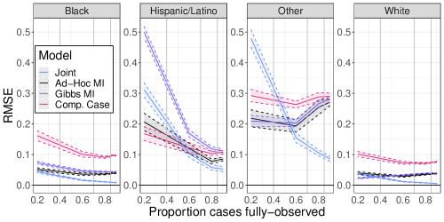
Figure 10: Root mean squared error across simulated datasets for the standardized incidence ratio, or $\text{SIR}_{j}$ for Blacks, Hispanic/Latinos, Others, and Whites plotted against the proportion of cases observed with race data. The blue color corresponds to the joint model in equation (11), while the red color corresponds to a the model defined in equation (15), or a complete-case analysis. Smaller magnitude is better.

F.2 80% posterior interval coverage

Table 9: Table shows 80% posterior credible interval coverages and lengths for estimands of interest from the simulation study. Coverage proportion is calculated across 200 simulated datasets for each model/simulation scenario. Column headers for percentages (e.g. 20%) indicate the missing-data simulation scenario which corresponds to the statistic calculated in the table column; the simulation scenario corresponds to the proportion of cases observed with completely observed race covariates.

		80% interval coverage				80% mean interval length
Parameter	Model	20%	60%	80%	90%	20%	60%	80%	90%
$\exp\big{(}(\boldsymbol{\alpha}_{\lambda})_{\text{Blacks}}$	Complete Case	0.70	0.70	0.68	0.60	0.51	0.47	0.47	0.44
$\quad\quad-(\boldsymbol{\alpha}_{\lambda})_{\text{Whites}}\big{)}$	Joint	0.78	0.81	0.81	0.78	0.62	0.55	0.55	0.53
	MI-Ad-hoc	1.00	0.88	0.77	0.66	0.41	0.40	0.43	0.42
	MI-Gibbs	0.75	0.70	0.67	0.61	0.52	0.46	0.46	0.44
$\exp\big{(}(\boldsymbol{\alpha}_{\lambda})_{\text{Hispanics/Latinos}}$	Complete Case	0.77	0.80	0.83	0.77	0.63	0.56	0.56	0.53
$\quad\quad-(\boldsymbol{\alpha}_{\lambda})_{\text{Whites}}\big{)}$	Joint	0.56	0.77	0.84	0.78	0.68	0.61	0.57	0.56
	MI-Ad-hoc	0.99	0.91	0.89	0.82	0.42	0.44	0.49	0.49
	MI-Gibbs	0.07	0.68	0.82	0.78	1.13	0.65	0.58	0.55
$\exp\big{(}(\boldsymbol{\alpha}_{\lambda})_{\text{Others}}$	Complete Case	0.42	0.33	0.27	0.28	0.44	0.38	0.37	0.36
$\quad\quad-(\boldsymbol{\alpha}_{\lambda})_{\text{Whites}}\big{)}$	Joint	0.37	0.73	0.77	0.82	0.63	0.67	0.60	0.58
	MI-Ad-hoc	1.00	0.62	0.41	0.30	0.40	0.36	0.36	0.35
	MI-Gibbs	0.70	0.48	0.32	0.29	0.71	0.42	0.39	0.37
$\mathbbm{SI}_{\text{Blacks}}$	Complete Case	0.06	0.04	0.01	0.00	0.03	0.02	0.01	0.01
	Joint	0.67	0.77	0.80	0.78	0.09	0.04	0.03	0.02
	MI-Ad-hoc	0.09	0.20	0.06	0.00	0.01	0.01	0.01	0.01
	MI-Gibbs	0.03	0.01	0.00	0.00	0.02	0.01	0.01	0.01
$\mathbbm{SI}_{\text{Hispanics/Latinos}}$	Complete Case	0.34	0.24	0.12	0.01	0.13	0.07	0.06	0.06
	Joint	0.46	0.74	0.81	0.70	0.47	0.23	0.14	0.10
	MI-Ad-hoc	0.12	0.23	0.27	0.06	0.07	0.06	0.06	0.06
	MI-Gibbs	0.00	0.05	0.01	0.01	0.16	0.08	0.06	0.06
$\mathbbm{SI}_{\text{Others}}$	Complete Case	0.03	0.00	0.00	0.00	0.11	0.06	0.05	0.05
	Joint	0.27	0.70	0.76	0.77	0.49	0.36	0.25	0.20
	MI-Ad-hoc	0.17	0.14	0.01	0.00	0.07	0.06	0.05	0.05
	MI-Gibbs	0.20	0.01	0.00	0.00	0.15	0.06	0.05	0.05
$\mathbbm{SI}_{\text{Whites}}$	Complete Case	0.04	0.01	0.00	0.00	0.02	0.01	0.01	0.01
	Joint	0.50	0.80	0.82	0.84	0.06	0.03	0.02	0.01
	MI-Ad-hoc	0.14	0.17	0.00	0.00	0.01	0.01	0.01	0.01
	MI-Gibbs	0.21	0.01	0.00	0.00	0.02	0.01	0.01	0.01
$\mathbbm{I}_{\text{Blacks}}/\mathbbm{I}_{\text{Whites}}$	Complete Case	0.06	0.01	0.00	0.00	0.04	0.02	0.02	0.02
	Joint	0.73	0.79	0.81	0.81	0.12	0.05	0.04	0.03
	MI-Ad-hoc	0.10	0.20	0.02	0.00	0.02	0.02	0.02	0.02
	MI-Gibbs	0.12	0.01	0.00	0.00	0.03	0.02	0.02	0.02
$\mathbbm{I}_{\text{Hispanics/Latinos}}/$	Complete Case	0.17	0.18	0.57	0.83	0.07	0.04	0.04	0.03
$\mathbbm{I}_{\text{Whites}}$	Joint	0.43	0.73	0.81	0.73	0.28	0.14	0.09	0.06
	MI-Ad-hoc	0.12	0.21	0.32	0.41	0.04	0.04	0.04	0.03
	MI-Gibbs	0.00	0.14	0.24	0.17	0.10	0.05	0.04	0.04
$\mathbbm{I}_{\text{Others}}/\mathbbm{I}_{\text{Whites}}$	Complete Case	0.00	0.00	0.00	0.00	0.06	0.03	0.03	0.03
	Joint	0.26	0.72	0.74	0.76	0.32	0.24	0.17	0.13
	MI-Ad-hoc	0.14	0.11	0.01	0.00	0.05	0.04	0.03	0.03
	MI-Gibbs	0.21	0.00	0.00	0.00	0.10	0.04	0.03	0.03

Table 10: Table shows 50% posterior credible interval coverages and lengths for estimands of interest from the simulation study. Coverage proportion is calculated across 200 simulated datasets for each model/simulation scenario. Column headers for percentages (e.g. 20%) indicate the missing-data simulation scenario which corresponds to the statistic calculated in the table column; the simulation scenario corresponds to the proportion of cases observed with completely observed race covariates.

		50% interval coverage				50% mean interval length
Parameter	Model	20%	60%	80%	90%	20%	60%	80%	90%
$\exp\big{(}(\boldsymbol{\alpha}_{\lambda})_{\text{Blacks}}$	Complete Case	0.39	0.35	0.41	0.32	0.27	0.24	0.24	0.23
$\quad\quad-(\boldsymbol{\alpha}_{\lambda})_{\text{Whites}}\big{)}$	Joint	0.52	0.53	0.49	0.47	0.32	0.28	0.29	0.27
	MI-Ad-hoc	0.96	0.56	0.47	0.30	0.21	0.21	0.22	0.22
	MI-Gibbs	0.48	0.38	0.38	0.29	0.27	0.24	0.24	0.23
$\exp\big{(}(\boldsymbol{\alpha}_{\lambda})_{\text{Hispanics/Latinos}}$	Complete Case	0.48	0.47	0.47	0.44	0.33	0.29	0.29	0.28
$\quad\quad-(\boldsymbol{\alpha}_{\lambda})_{\text{Whites}}\big{)}$	Joint	0.27	0.48	0.47	0.43	0.35	0.31	0.30	0.29
	MI-Ad-hoc	0.96	0.62	0.53	0.47	0.22	0.23	0.25	0.25
	MI-Gibbs	0.01	0.39	0.46	0.45	0.58	0.33	0.30	0.28
$\exp\big{(}(\boldsymbol{\alpha}_{\lambda})_{\text{Others}}$	Complete Case	0.20	0.10	0.12	0.09	0.23	0.20	0.19	0.19
$\quad\quad-(\boldsymbol{\alpha}_{\lambda})_{\text{Whites}}\big{)}$	Joint	0.17	0.41	0.47	0.51	0.32	0.35	0.31	0.30
	MI-Ad-hoc	0.91	0.29	0.15	0.10	0.21	0.18	0.19	0.18
	MI-Gibbs	0.38	0.23	0.12	0.10	0.36	0.22	0.20	0.19
$\mathbbm{SI}_{\text{Blacks}}$	Complete Case	0.04	0.02	0.00	0.00	0.01	0.01	0.01	0.01
	Joint	0.39	0.49	0.48	0.49	0.04	0.02	0.01	0.01
	MI-Ad-hoc	0.04	0.09	0.03	0.00	0.01	0.01	0.01	0.01
	MI-Gibbs	0.03	0.01	0.00	0.00	0.01	0.01	0.01	0.01
$\mathbbm{SI}_{\text{Hispanics/Latinos}}$	Complete Case	0.17	0.12	0.05	0.00	0.07	0.04	0.03	0.03
	Joint	0.27	0.47	0.51	0.41	0.24	0.12	0.07	0.05
	MI-Ad-hoc	0.07	0.15	0.18	0.01	0.04	0.03	0.03	0.03
	MI-Gibbs	0.00	0.01	0.01	0.00	0.08	0.04	0.03	0.03
$\mathbbm{SI}_{\text{Others}}$	Complete Case	0.01	0.00	0.00	0.00	0.06	0.03	0.03	0.02
	Joint	0.12	0.45	0.48	0.41	0.25	0.18	0.13	0.10
	MI-Ad-hoc	0.08	0.07	0.01	0.00	0.04	0.03	0.03	0.03
	MI-Gibbs	0.09	0.00	0.00	0.00	0.08	0.03	0.03	0.02
$\mathbbm{SI}_{\text{Whites}}$	Complete Case	0.03	0.01	0.00	0.00	0.01	0.01	0.00	0.00
	Joint	0.28	0.51	0.54	0.51	0.03	0.02	0.01	0.01
	MI-Ad-hoc	0.07	0.08	0.00	0.00	0.01	0.00	0.00	0.00
	MI-Gibbs	0.08	0.00	0.00	0.00	0.01	0.01	0.00	0.00
$\mathbbm{I}_{\text{Blacks}}/\mathbbm{I}_{\text{Whites}}$	Complete Case	0.03	0.01	0.00	0.00	0.02	0.01	0.01	0.01
	Joint	0.48	0.54	0.52	0.48	0.06	0.03	0.02	0.01
	MI-Ad-hoc	0.04	0.10	0.01	0.00	0.01	0.01	0.01	0.01
	MI-Gibbs	0.07	0.01	0.00	0.00	0.02	0.01	0.01	0.01
$\mathbbm{I}_{\text{Hispanics/Latinos}}/$	Complete Case	0.09	0.08	0.33	0.53	0.03	0.02	0.02	0.02
$\mathbbm{I}_{\text{Whites}}$	Joint	0.24	0.46	0.51	0.45	0.14	0.07	0.05	0.03
	MI-Ad-hoc	0.09	0.12	0.17	0.24	0.02	0.02	0.02	0.02
	MI-Gibbs	0.00	0.09	0.07	0.05	0.05	0.02	0.02	0.02
$\mathbbm{I}_{\text{Others}}/\mathbbm{I}_{\text{Whites}}$	Complete Case	0.00	0.00	0.00	0.00	0.03	0.02	0.02	0.01
	Joint	0.12	0.43	0.47	0.41	0.16	0.12	0.09	0.07
	MI-Ad-hoc	0.09	0.06	0.00	0.00	0.02	0.02	0.02	0.02
	MI-Gibbs	0.09	0.00	0.00	0.00	0.05	0.02	0.02	0.02

Appendix G Prior sensitivity graphs

Graphs to support conclusions in 3.7

Appendix H Further Wayne County applied data analysis results

H.1 Age-Race/Ethnicity posterior predictive checks

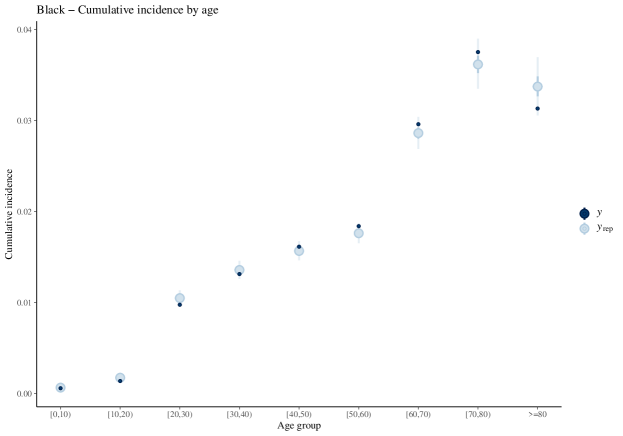
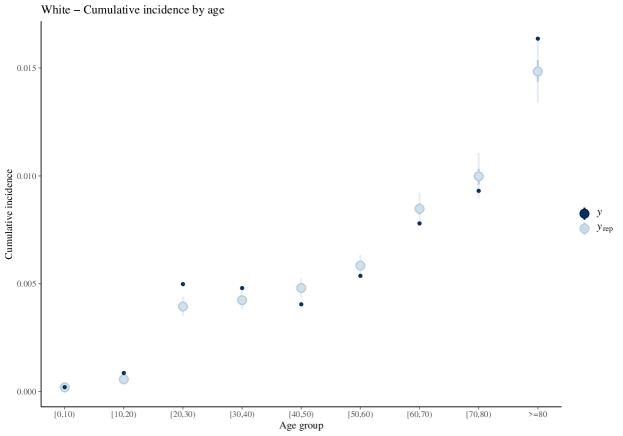
Figure 16: Posterior predictive checks for cumulative incidence by age group by race for Blacks and Whites.

H.2 Rootogram

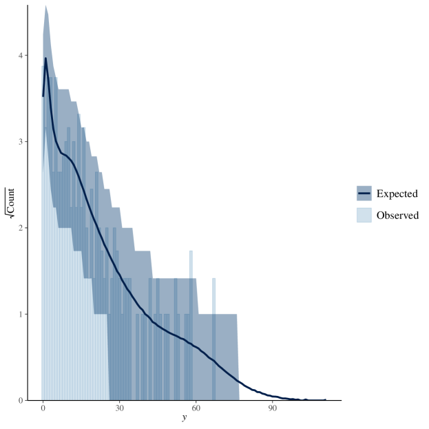
Figure 17: Posterior predictive rootogram for missing case counts.

H.3 Tables for posterior summaries for estimands of interest

Table 11: This table presents posterior summary statistics for the Wayne-County estimands of interest. Post. mean stands for Posterior Mean, and MCSE stands for Monte Carlo Standard Error, which is the standard error in the posterior estimator, which can be estimated assuming that the MCMC central limit theorem holds. See Betancourt and Girolami (2015) and Vehtari et al. (2020) for more details

		Post.		10% Post.		90% Post.
Estimand	Model	Mean	MCSE	quant.	MCSE	quant.	MCSE
$\exp\big{(}(\boldsymbol{\alpha}_{\lambda})_{\text{Blacks}}$	Joint	3.93	1.28e-02	3.16	1.40e-02	4.76	2.06e-02
$\quad\quad-(\boldsymbol{\alpha}_{\lambda})_{\text{Whites}}\big{)}$	Complete Case model	3.56	1.02e-02	2.89	1.09e-02	4.29	1.79e-02
	Ad-Hoc MI	2.96	1.80e-03	2.43	1.60e-03	3.52	2.15e-03
	Gibbs MI	3.49	1.75e-03	2.78	1.84e-03	4.24	2.59e-03
$\exp\big{(}(\boldsymbol{\alpha}_{\lambda})_{\text{Hispanics/Latinos}}$	Joint	2.10	6.34e-03	1.65	6.39e-03	2.59	8.22e-03
$\quad\quad-(\boldsymbol{\alpha}_{\lambda})_{\text{Whites}}\big{)}$	Complete Case model	1.93	4.35e-03	1.58	4.66e-03	2.29	8.52e-03
	Ad-Hoc MI	1.67	1.83e-03	1.35	1.72e-03	2.01	1.55e-03
	Gibbs MI	2.09	3.22e-03	1.65	2.62e-03	2.56	3.87e-03
$\exp\big{(}(\boldsymbol{\alpha}_{\lambda})_{\text{Others}}$	Joint	8.88	4.78e-02	6.09	5.51e-02	11.81	6.13e-02
$\quad\quad-(\boldsymbol{\alpha}_{\lambda})_{\text{Whites}}\big{)}$	Complete Case model	5.21	1.30e-02	4.26	1.55e-02	6.22	1.91e-02
	Ad-Hoc MI	4.08	2.75e-03	3.32	2.52e-03	4.90	2.79e-03
	Gibbs MI	5.27	5.03e-03	4.18	4.14e-03	6.42	4.88e-03
$\exp\big{(}(\boldsymbol{\alpha}_{\lambda})_{\text{Asians/Pacific Islanders}}$	Joint	1.35	4.79e-03	1.01	5.14e-03	1.73	7.37e-03
$\quad\quad-(\boldsymbol{\alpha}_{\lambda})_{\text{Whites}}\big{)}$	Complete Case model	1.29	3.30e-03	1.00	3.59e-03	1.61	6.06e-03
	Ad-Hoc MI	1.21	1.98e-03	0.96	1.63e-03	1.48	2.43e-03
	Gibbs MI	1.66	4.44e-03	1.22	3.10e-03	2.15	6.17e-03
$\mathbbm{SI}_{\text{Blacks}}$	Joint	1.59	6.62e-04	1.55	1.20e-03	1.64	7.33e-04
	Complete Case model	1.58	8.02e-05	1.57	1.44e-04	1.60	1.53e-04
	Ad-Hoc MI	1.56	1.47e-04	1.55	1.63e-04	1.57	1.37e-04
	Gibbs MI	1.60	1.65e-04	1.58	1.72e-04	1.61	1.65e-04
$\mathbbm{SI}_{\text{Hispanics/Latinos}}$	Joint	1.16	1.59e-03	1.02	1.55e-03	1.30	2.20e-03
	Complete Case model	1.17	3.29e-04	1.12	6.04e-04	1.23	6.36e-04
	Ad-Hoc MI	1.15	7.02e-04	1.10	6.59e-04	1.20	7.41e-04
	Gibbs MI	1.23	9.89e-04	1.17	1.05e-03	1.28	1.01e-03
$\mathbbm{SI}_{\text{Others}}$	Joint	4.64	1.81e-02	3.50	2.24e-02	5.64	1.38e-02
	Complete Case model	3.06	8.03e-04	2.93	1.33e-03	3.19	1.77e-03
	Ad-Hoc MI	2.68	1.21e-03	2.57	1.03e-03	2.80	1.38e-03
	Gibbs MI	3.15	2.40e-03	3.01	NA	3.28	2.69e-03
$\mathbbm{SI}_{\text{Asians/Pacific Islanders}}$	Joint	0.61	1.09e-03	0.53	4.95e-04	0.71	2.52e-03
	Complete Case model	0.65	3.27e-04	0.60	7.57e-04	0.71	7.64e-04
	Ad-Hoc MI	0.66	8.58e-04	0.61	8.63e-04	0.72	9.36e-04
	Gibbs MI	0.72	1.14e-03	0.66	NA	0.78	1.34e-03
$\mathbbm{SI}_{\text{Whites}}$	Joint	0.46	4.25e-04	0.44	3.98e-04	0.49	4.65e-04
	Complete Case model	0.52	5.20e-05	0.52	7.63e-05	0.53	1.08e-04
	Ad-Hoc MI	0.55	1.00e-04	0.54	9.79e-05	0.56	1.02e-04
	Gibbs MI	0.50	9.26e-05	0.49	1.11e-04	0.51	8.00e-05
$\mathbbm{I}_{\text{Blacks}}/\mathbbm{I}_{\text{Whites}}$	Joint	3.01	2.86e-03	2.84	2.98e-03	3.19	3.31e-03
	Complete Case model	2.63	3.77e-04	2.57	5.53e-04	2.70	7.52e-04
	Ad-Hoc MI	2.49	6.53e-04	2.44	6.89e-04	2.55	6.51e-04
	Gibbs MI	2.79	7.12e-04	2.73	6.31e-04	2.85	8.37e-04
$\mathbbm{I}_{\text{Hispanics/Latinos}}/$	Joint	1.69	3.26e-03	1.47	3.26e-03	1.92	4.36e-03
$\mathbbm{I}_{\text{Whites}}$	Complete Case model	1.50	4.66e-04	1.42	9.17e-04	1.58	1.13e-03
	Ad-Hoc MI	1.42	9.31e-04	1.35	9.26e-04	1.49	9.86e-04
	Gibbs MI	1.66	1.43e-03	1.57	1.44e-03	1.74	1.50e-03
$\mathbbm{I}_{\text{Others}}/\mathbbm{I}_{\text{Whites}}$	Joint	6.55	2.96e-02	4.74	3.24e-02	8.12	2.06e-02
	Complete Case model	3.78	1.11e-03	3.60	2.05e-03	3.96	2.31e-03
	Ad-Hoc MI	3.20	1.67e-03	3.04	1.40e-03	3.35	1.90e-03
	Gibbs MI	4.10	3.36e-03	3.90	NA	4.30	4.10e-03
$\mathbbm{I}_{\text{Asians/Pacific Islanders}}/$	Joint	1.08	2.59e-03	0.92	1.60e-03	1.27	5.65e-03
$\mathbbm{I}_{\text{Whites}}$	Complete Case model	1.01	5.26e-04	0.92	1.04e-03	1.10	1.02e-03
	Ad-Hoc MI	0.99	1.32e-03	0.91	NA	1.07	1.39e-03
	Gibbs MI	1.18	1.89e-03	1.08	NA	1.28	2.25e-03

Table 12: The table shows sampling efficiency for population estimands of interest presented in table 11. ESS stands for effective sample size; Bulk ESS and Tail ESS are measures of the equivalent number of independent samples generated from a MCMC procedure. See Vehtari et al. (2020) for more detail. Bulk and Tail ESS efficiency are the Bulk and Tail ESS figures divided by the total number of MCMC samples, which is $16,000$. As noted in Vehtari et al. (2020) it is possible for MCMC samplers to generate Tail and Bulk ESS values that are larger than the total number of samples.

Estimand	Model	$\hat{R}$	Bulk ESS	Tail ESS	Bulk ESS eff.	Tail ESS eff.
$\exp\big{(}(\boldsymbol{\alpha}_{\lambda})_{\text{Blacks}}$	Joint	1.00	2465	4753	0.15	0.30
$\quad\quad-(\boldsymbol{\alpha}_{\lambda})_{\text{Whites}}\big{)}$	Complete Case model	1.00	3037	5645	0.19	0.35
	Ad-Hoc MI	1.01	57036	223009	0.07	0.28
	Gibbs MI	1.00	114009	259368	0.14	0.32
$\exp\big{(}(\boldsymbol{\alpha}_{\lambda})_{\text{Hispanics/Latinos}}$	Joint	1.00	3506	6994	0.22	0.44
$\quad\quad-(\boldsymbol{\alpha}_{\lambda})_{\text{Whites}}\big{)}$	Complete Case model	1.00	4440	6910	0.28	0.43
	Ad-Hoc MI	1.01	19965	91952	0.02	0.11
	Gibbs MI	1.02	12435	68983	0.02	0.09
$\exp\big{(}(\boldsymbol{\alpha}_{\lambda})_{\text{Others}}$	Joint	1.00	2098	4315	0.13	0.27
$\quad\quad-(\boldsymbol{\alpha}_{\lambda})_{\text{Whites}}\big{)}$	Complete Case model	1.00	3742	6528	0.23	0.41
	Ad-Hoc MI	1.01	51519	256045	0.06	0.32
	Gibbs MI	1.01	30320	220330	0.04	0.28
$\exp\big{(}(\boldsymbol{\alpha}_{\lambda})_{\text{Asians/Pacific Islanders}}$	Joint	1.00	3850	7799	0.24	0.49
$\quad\quad-(\boldsymbol{\alpha}_{\lambda})_{\text{Whites}}\big{)}$	Complete Case model	1.00	5511	8283	0.34	0.52
	Ad-Hoc MI	1.02	11078	45632	0.01	0.06
	Gibbs MI	1.03	7298	30332	0.01	0.04
$\mathbbm{SI}_{\text{Blacks}}$	Joint	1.00	2531	4877	0.16	0.30
	Complete Case model	1.00	16204	14672	1.01	0.92
	Ad-Hoc MI	1.05	4322	15046	0.01	0.02
	Gibbs MI	1.06	3490	13738	0.00	0.02
$\mathbbm{SI}_{\text{Hispanics/Latinos}}$	Joint	1.00	4523	9442	0.28	0.59
	Complete Case model	1.00	16596	12657	1.04	0.79
	Ad-Hoc MI	1.07	3392	14038	0.00	0.02
	Gibbs MI	1.12	1990		0.00	NA
$\mathbbm{SI}_{\text{Others}}$	Joint	1.00	2034	4928	0.13	0.31
	Complete Case model	1.00	16338	11881	1.02	0.74
	Ad-Hoc MI	1.04	5584	18672	0.01	0.02
	Gibbs MI	1.12	1938		0.00	NA
$\mathbbm{SI}_{\text{Asians/Pacific Islanders}}$	Joint	1.00	6412	6513	0.40	0.41
	Complete Case model	1.00	17496	11891	1.09	0.74
	Ad-Hoc MI	1.10	2439		0.00	NA
	Gibbs MI	1.15	1673		0.00	NA
$\mathbbm{SI}_{\text{Whites}}$	Joint	1.00	1722	5572	0.11	0.35
	Complete Case model	1.00	16277	13527	1.02	0.85
	Ad-Hoc MI	1.05	4083	17557	0.01	0.02
	Gibbs MI	1.05	4488		0.01	NA
$\mathbbm{I}_{\text{Blacks}}/\mathbbm{I}_{\text{Whites}}$	Joint	1.00	2197	5606	0.14	0.35
	Complete Case model	1.00	16184	13675	1.01	0.85
	Ad-Hoc MI	1.05	4225	16200	0.01	0.02
	Gibbs MI	1.05	4673		0.01	NA
$\mathbbm{I}_{\text{Hispanics/Latinos}}/$	Joint	1.00	2928	6147	0.18	0.38
$\mathbbm{I}_{\text{Whites}}$	Complete Case model	1.00	16631	12370	1.04	0.77
	Ad-Hoc MI	1.06	3557	14586	0.00	0.02
	Gibbs MI	1.11	2144		0.00	NA
$\mathbbm{I}_{\text{Others}}/\mathbbm{I}_{\text{Whites}}$	Joint	1.00	1933	4788	0.12	0.30
	Complete Case model	1.00	16306	11978	1.02	0.75
	Ad-Hoc MI	1.04	5156		0.01	NA
	Gibbs MI	1.11	2114		0.00	NA
$\mathbbm{I}_{\text{Asians/Pacific Islanders}}/$	Joint	1.00	3827	6402	0.24	0.40
$\mathbbm{I}_{\text{Whites}}$	Complete Case model	1.00	17423	11926	1.09	0.75
	Ad-Hoc MI	1.10	2447		0.00	NA
	Gibbs MI	1.14	1731		0.00	NA

Table 13: The table shows the posterior means, 80% credible interval endpoints and the Monte Carlo standard errors of these estimates. CC stands for the complete-case model while J stands for the joint model.

	Post.		10% Post.		90% Post.
Estimand	Mean	MCSE	quant.	MCSE	quant.	MCSE
$\mathbb{I}^{\text{CC}}_{\text{Blacks}}/\mathbb{I}^{\text{J}}_{\text{Blacks}}$	0.81	3.50e-04	0.79	3.55e-04	0.84	5.80e-04
$\mathbb{I}^{\text{CC}}_{\text{Hispanics/Latinos}}/\mathbb{I}^{\text{J}}_{\text{Hispanics/Latinos}}$	0.83	1.14e-03	0.73	1.14e-03	0.94	1.70e-03
$\mathbb{I}^{\text{CC}}_{\text{Others}}/\mathbb{I}^{\text{J}}_{\text{Others}}$	0.55	2.41e-03	0.44	1.36e-03	0.71	4.26e-03
$\mathbb{I}^{\text{CC}}_{\text{Asians/Pacific Islanders}}/\mathbb{I}^{\text{J}}_{\text{Asians/Pacific Islanders}}$	0.88	1.42e-03	0.73	2.50e-03	1.03	1.71e-03
$\mathbb{I}^{\text{CC}}_{\text{Whites}}/\mathbb{I}^{\text{J}}_{\text{Whites}}$	0.93	8.51e-04	0.88	7.85e-04	0.98	7.79e-04
$\Pb\left(\text{Race observed}\right)_{\text{Blacks}}$	0.85	7.55e-04	0.81	7.25e-04	0.91	1.35e-03
$\Pb\left(\text{Race observed}\right)_{\text{Hispanics/Latinos}}$	0.87	8.63e-04	0.78	1.43e-03	0.95	6.59e-04
$\Pb\left(\text{Race observed}\right)_{\text{Others}}$	0.58	2.93e-03	0.45	1.20e-03	0.77	5.31e-03
$\Pb\left(\text{Race observed}\right)_{\text{Asians/Pacific Islanders}}$	0.90	8.25e-04	0.81	2.36e-03	0.97	3.80e-04
$\Pb\left(\text{Race observed}\right)_{\text{Whites}}$	0.94	7.09e-04	0.89	8.70e-04	0.98	4.33e-04

Appendix I Stan code for negative binomial likelihood

The following Stan code computes the likelihood related to the following generative model using an efficient dynamic programming algorithm :

$$Y_{ij} \sim\text{Binomial}(E_{ij},\theta_{ij})$$

$$X_{ij}|Y_{ij} \sim\text{Binomial}(Y_{ij},p_{ij})$$

after marginalizing over all combinations of $Y_{ij}$ such that $\sum_{j}Y_{ij}=T$ where $T$ is the total identified cases of disease in stratum $i$, a known quantity.

The code was derived from Carpenter (2018).

⬇

functions {

real binomial_2_lpmf(int y_obs, int y_miss,

real p, real theta, int E) {

return binomial_lpmf(y_obs | y_miss, p)

+ binomial_lpmf(y_miss | E, theta);

}

real miss_lpmf(int[] y, int n_miss,

vector p, vector theta,

int[] E) {

int N = rows(theta);

real alpha[N + 1, n_miss + 1];

// alpha[n + 1, tot + 1] = log p of tot missing cases

// distributed among first n categories

alpha[1, 1:(n_miss + 1)] = rep_array(0, n_miss+1);

for (n in 1:N) {

// tot = 0

alpha[n + 1, 1] = alpha[n, 1]

+ binomial_2_lpmf(y[n]|y[n],p[n],theta[n], E[n]);

// 0 < tot < n

for (tot in 1:n_miss) {

if (n > 1) {

vector[tot + 1] vec;

for (i in 1:(tot + 1)) {

vec[i] = alpha[n,i]

+ binomial_2_lpmf(y[n] |

y[n] + tot - (i - 1),

p[n],theta[n], E[n]);

}

alpha[n + 1, tot + 1] = log_sum_exp(vec);

} else {

alpha[n + 1,tot + 1]

= binomial_2_lpmf(y[n]| y[n]

+ tot,p[n],theta[n], E[n]);

}

}

}

return alpha[N + 1, n_miss + 1];

}

}

[Acknowledgments] We would like to thank Mitzi Morris, Andrew Gelman, and Bob Carpenter for their feedback on an earlier draft of the paper.

JZ & RT were supported by award #6 U01 IP00113801-01 from the U.S. Centers for Disease Control and Prevention, and award #812255 from the Simons Foundation. This research was supported in part through computational resources and services provided by Advanced Research Computing (ARC), a division of Information and Technology Services (ITS) at the University of Michigan, Ann Arbor.

References

- Aguayo et al. (2020) {barticle}[author] \bauthor\bsnmAguayo, \bfnmGloria A.\binitsG. A., \bauthor\bsnmSchritz, \bfnmAnna\binitsA., \bauthor\bsnmRuiz-Castell, \bfnmMaria\binitsM., \bauthor\bsnmVillarroel, \bfnmLuis\binitsL., \bauthor\bsnmValdivia, \bfnmGonzalo\binitsG., \bauthor\bsnmFagherazzi, \bfnmGuy\binitsG., \bauthor\bsnmWitte, \bfnmDaniel R.\binitsD. R. and \bauthor\bsnmLawson, \bfnmAndrew\binitsA. (\byear2020). \btitleIdentifying Hotspots of Cardiometabolic Outcomes Based on a Bayesian Approach: The Example of Chile. \bjournalPLOS ONE \bvolume15. \bdoi10.1371/journal.pone.0235009 \endbibitem
- Audigier et al. (2018) {barticle}[author] \bauthor\bsnmAudigier, \bfnmVincent\binitsV., \bauthor\bsnmWhite, \bfnmIan R\binitsI. R., \bauthor\bsnmJolani, \bfnmShahab\binitsS., \bauthor\bsnmDebray, \bfnmThomas PA\binitsT. P., \bauthor\bsnmQuartagno, \bfnmMatteo\binitsM., \bauthor\bsnmCarpenter, \bfnmJames\binitsJ., \bauthor\bsnmVan Buuren, \bfnmStef\binitsS. and \bauthor\bsnmResche-Rigon, \bfnmMatthieu\binitsM. (\byear2018). \btitleMultiple imputation for multilevel data with continuous and binary variables. \bjournalStatistical Science \bvolume33 \bpages160–183. \endbibitem
- Baker, White and Mengersen (2014) {barticle}[author] \bauthor\bsnmBaker, \bfnmJannah\binitsJ., \bauthor\bsnmWhite, \bfnmNicole\binitsN. and \bauthor\bsnmMengersen, \bfnmKerrie\binitsK. (\byear2014). \btitleMissing in Space: An Evaluation of Imputation Methods for Missing Data in Spatial Analysis of Risk Factors for Type II Diabetes. \bvolume13. \bdoi10.1186/1476-072X-13-47 \endbibitem
- Bauer and Wakefield (2018) {barticle}[author] \bauthor\bsnmBauer, \bfnmCici\binitsC. and \bauthor\bsnmWakefield, \bfnmJon\binitsJ. (\byear2018). \btitleStratified Space–Time Infectious Disease Modelling, with an Application to Hand, Foot and Mouth Disease in China. \bjournalJournal of the Royal Statistical Society Series C \bvolume67. \endbibitem
- Betancourt (2018) {barticle}[author] \bauthor\bsnmBetancourt, \bfnmMichael\binitsM. (\byear2018). \btitleA Conceptual Introduction to Hamiltonian Monte Carlo. \bjournalarXiv:1701.02434 [stat]. \endbibitem
- Betancourt and Girolami (2015) {barticle}[author] \bauthor\bsnmBetancourt, \bfnmMichael\binitsM. and \bauthor\bsnmGirolami, \bfnmMark\binitsM. (\byear2015). \btitleHamiltonian Monte Carlo for hierarchical models. \bjournalCurrent trends in Bayesian methodology with applications \bvolume79 \bpages2–4. \endbibitem
- Bilal et al. (2021) {barticle}[author] \bauthor\bsnmBilal, \bfnmUsama\binitsU., \bauthor\bsnmTabb, \bfnmLoni P\binitsL. P., \bauthor\bsnmBarber, \bfnmSharrelle\binitsS. and \bauthor\bsnmDiez Roux, \bfnmAna V\binitsA. V. (\byear2021). \btitleSpatial Inequities in COVID-19 Testing, Positivity, Confirmed Cases, and Mortality in 3 US Cities: An Ecological Study. \bjournalAnnals of internal medicine. \endbibitem
- Bürkner et al. (2021) {bmisc}[author] \bauthor\bsnmBürkner, \bfnmPaul-Christian\binitsP.-C., \bauthor\bsnmGabry, \bfnmJonah\binitsJ., \bauthor\bsnmKay, \bfnmMatthew\binitsM. and \bauthor\bsnmVehtari, \bfnmAki\binitsA. (\byear2021). \btitleposterior: Tools for Working with Posterior Distributions. \bnoteR package version 1.0.1. \endbibitem
- Carpenter (2018) {bmisc}[author] \bauthor\bsnmCarpenter, \bfnmBob\binitsB. (\byear2018). \btitleStan Implementation of Poisson-binomial distribution. \bhowpublishedhttps://discourse.mc-stan.org/t/poisson-binomial-distribution-any-existing-stan-implementation/4220/7. \bnoteAccessed: 2022-02-10. \endbibitem
- Catchpole (1997) {barticle}[author] \bauthor\bsnmCatchpole, \bfnmE.\binitsE. (\byear1997). \btitleDetecting Parameter Redundancy. \bvolume84 \bpages187–196. \bdoi10.1093/biomet/84.1.187 \endbibitem
- Clark and Houle (2014) {barticle}[author] \bauthor\bsnmClark, \bfnmSamuel J\binitsS. J. and \bauthor\bsnmHoule, \bfnmBrian\binitsB. (\byear2014). \btitleValidation, replication, and sensitivity testing of Heckman-type selection models to adjust estimates of HIV prevalence. \bjournalPloS one \bvolume9 \bpagese112563. \endbibitem
- Cook, Gelman and Rubin (2006) {barticle}[author] \bauthor\bsnmCook, \bfnmSamantha R\binitsS. R., \bauthor\bsnmGelman, \bfnmAndrew\binitsA. and \bauthor\bsnmRubin, \bfnmDonald B\binitsD. B. (\byear2006). \btitleValidation of software for Bayesian models using posterior quantiles. \bjournalJournal of Computational and Graphical Statistics \bvolume15 \bpages675–692. \endbibitem
- Diggle and Kenward (1994) {barticle}[author] \bauthor\bsnmDiggle, \bfnmPeter\binitsP. and \bauthor\bsnmKenward, \bfnmMichael G\binitsM. G. (\byear1994). \btitleInformative drop-out in longitudinal data analysis. \bjournalJournal of the Royal Statistical Society: Series C (Applied Statistics) \bvolume43 \bpages49–73. \endbibitem
- Eekhout et al. (2012) {barticle}[author] \bauthor\bsnmEekhout, \bfnmIris\binitsI., \bauthor\bparticlede \bsnmBoer, \bfnmR. Michiel\binitsR. M., \bauthor\bsnmTwisk, \bfnmJos W. R.\binitsJ. W. R., \bauthor\bparticlede \bsnmVet, \bfnmHenrica C. W.\binitsH. C. W. and \bauthor\bsnmHeymans, \bfnmMartijn W.\binitsM. W. (\byear2012). \btitleMissing Data: A Systematic Review of How They Are Reported and Handled. \bvolume23. \bdoi10.1097/EDE.0b013e3182576cdb \endbibitem
- Elliott et al. (2009) {barticle}[author] \bauthor\bsnmElliott, \bfnmMarc N.\binitsM. N., \bauthor\bsnmMorrison, \bfnmPeter A.\binitsP. A., \bauthor\bsnmFremont, \bfnmAllen\binitsA., \bauthor\bsnmMcCaffrey, \bfnmDaniel F.\binitsD. F., \bauthor\bsnmPantoja, \bfnmPhilip\binitsP. and \bauthor\bsnmLurie, \bfnmNicole\binitsN. (\byear2009). \btitleUsing the Census Bureau’s Surname List to Improve Estimates of Race/Ethnicity and Associated Disparities. \bvolume9. \bdoi10.1007/s10742-009-0047-1 \endbibitem
- Frome (1983) {barticle}[author] \bauthor\bsnmFrome, \bfnmE. L.\binitsE. L. (\byear1983). \btitleThe Analysis of Rates Using Poisson Regression Models. \bjournalBiometrics \bvolume39. \bdoi10.2307/2531094 \endbibitem
- Frome and Checkoway (1985) {barticle}[author] \bauthor\bsnmFrome, \bfnmEdward L.\binitsE. L. and \bauthor\bsnmCheckoway, \bfnmHarvey\binitsH. (\byear1985). \btitleUSE OF POISSON REGRESSION MODELS IN ESTIMATING INCIDENCE RATES AND RATIOS. \bjournalAmerican Journal of Epidemiology \bvolume121. \bdoi10.1093/oxfordjournals.aje.a114001 \endbibitem
- Gabry and Mahr (2021) {bmisc}[author] \bauthor\bsnmGabry, \bfnmJonah\binitsJ. and \bauthor\bsnmMahr, \bfnmTristan\binitsT. (\byear2021). \btitlebayesplot: Plotting for Bayesian Models. \bnoteR package version 1.8.1. \endbibitem
- Gabry et al. (2019) {barticle}[author] \bauthor\bsnmGabry, \bfnmJonah\binitsJ., \bauthor\bsnmSimpson, \bfnmDaniel\binitsD., \bauthor\bsnmVehtari, \bfnmAki\binitsA., \bauthor\bsnmBetancourt, \bfnmMichael\binitsM. and \bauthor\bsnmGelman, \bfnmAndrew\binitsA. (\byear2019). \btitleVisualization in Bayesian workflow. \bjournalJ. R. Stat. Soc. A \bvolume182 \bpages389-402. \bdoi10.1111/rssa.12378 \endbibitem
- Gabry and Češnovar (2021) {bmanual}[author] \bauthor\bsnmGabry, \bfnmJonah\binitsJ. and \bauthor\bsnmČešnovar, \bfnmRok\binitsR. (\byear2021). \btitlecmdstanr: R Interface to ’CmdStan’ \bnotehttps://mc-stan.org/cmdstanr, https://discourse.mc-stan.org. \endbibitem
- Gao et al. (2021) {barticle}[author] \bauthor\bsnmGao, \bfnmYuxiang\binitsY., \bauthor\bsnmKennedy, \bfnmLauren\binitsL., \bauthor\bsnmSimpson, \bfnmDaniel\binitsD. and \bauthor\bsnmGelman, \bfnmAndrew\binitsA. (\byear2021). \btitleImproving Multilevel Regression and Poststratification with Structured Priors. \bjournalBayesian Analysis \bvolume-1. \bdoi10.1214/20-BA1223 \endbibitem
- Gelman and Little (1997) {barticle}[author] \bauthor\bsnmGelman, \bfnmAndrew\binitsA. and \bauthor\bsnmLittle, \bfnmThomas C\binitsT. C. (\byear1997). \btitlePoststratification into many categories using hierarchical logistic regression. \endbibitem
- Gelman, Simpson and Betancourt (2017) {barticle}[author] \bauthor\bsnmGelman, \bfnmAndrew\binitsA., \bauthor\bsnmSimpson, \bfnmDaniel\binitsD. and \bauthor\bsnmBetancourt, \bfnmMichael\binitsM. (\byear2017). \btitleThe Prior Can Often Only Be Understood in the Context of the Likelihood. \bjournalEntropy \bvolume19. \bdoi10.3390/e19100555 \endbibitem
- Gelman et al. (2013) {barticle}[author] \bauthor\bsnmGelman, \bfnmAndrew\binitsA., \bauthor\bsnmCarlin, \bfnmJohn B\binitsJ. B., \bauthor\bsnmStern, \bfnmHal S\binitsH. S., \bauthor\bsnmDunson, \bfnmDavid B\binitsD. B., \bauthor\bsnmVehtari, \bfnmAki\binitsA. and \bauthor\bsnmRubin, \bfnmDonald B\binitsD. B. (\byear2013). \btitleBayesian Data Analysis. \endbibitem
- Gelman et al. (2020) {barticle}[author] \bauthor\bsnmGelman, \bfnmAndrew\binitsA., \bauthor\bsnmVehtari, \bfnmAki\binitsA., \bauthor\bsnmSimpson, \bfnmDaniel\binitsD., \bauthor\bsnmMargossian, \bfnmCharles C\binitsC. C., \bauthor\bsnmCarpenter, \bfnmBob\binitsB., \bauthor\bsnmYao, \bfnmYuling\binitsY., \bauthor\bsnmKennedy, \bfnmLauren\binitsL., \bauthor\bsnmGabry, \bfnmJonah\binitsJ., \bauthor\bsnmBürkner, \bfnmPaul-Christian\binitsP.-C. and \bauthor\bsnmModrák, \bfnmMartin\binitsM. (\byear2020). \btitleBayesian workflow. \bjournalarXiv preprint arXiv:2011.01808. \endbibitem
- Gómez-Rubio, Cameletti and Blangiardo (2019) {barticle}[author] \bauthor\bsnmGómez-Rubio, \bfnmVirgilio\binitsV., \bauthor\bsnmCameletti, \bfnmMichela\binitsM. and \bauthor\bsnmBlangiardo, \bfnmMarta\binitsM. (\byear2019). \btitleMissing Data Analysis and Imputation via Latent Gaussian Markov Random Fields. \endbibitem
- Gustafson (2015) {bbook}[author] \bauthor\bsnmGustafson, \bfnmPaul\binitsP. (\byear2015). \btitleBayesian inference for partially identified models: Exploring the limits of limited data \bvolume140. \bpublisherCRC Press. \endbibitem
- Held and Paul (2012) {barticle}[author] \bauthor\bsnmHeld, \bfnmLeonhard\binitsL. and \bauthor\bsnmPaul, \bfnmMichaela\binitsM. (\byear2012). \btitleModeling Seasonality in Space-Time Infectious Disease Surveillance Data: Modeling Seasonality in Space-Time Data. \bjournalBiometrical Journal \bvolume54. \bdoi10.1002/bimj.201200037 \endbibitem
- Held et al. (2019) {bbook}[author] \bauthor\bsnmHeld, \bfnmLeonhard\binitsL., \bauthor\bsnmHens, \bfnmNiel\binitsN., \bauthor\bsnmD O’Neill, \bfnmPhilip\binitsP. and \bauthor\bsnmWallinga, \bfnmJacco\binitsJ. (\byear2019). \btitleHandbook of infectious disease data analysis. \bpublisherCRC Press. \endbibitem
- Hoffman et al. (2014) {barticle}[author] \bauthor\bsnmHoffman, \bfnmMatthew D\binitsM. D., \bauthor\bsnmGelman, \bfnmAndrew\binitsA. \betalet al. (\byear2014). \btitleThe No-U-Turn sampler: adaptively setting path lengths in Hamiltonian Monte Carlo. \bjournalJ. Mach. Learn. Res. \bvolume15 \bpages1593–1623. \endbibitem
- Holland, Jones and Benschop (2015) {barticle}[author] \bauthor\bsnmHolland, \bfnmR. C.\binitsR. C., \bauthor\bsnmJones, \bfnmG.\binitsG. and \bauthor\bsnmBenschop, \bfnmJ.\binitsJ. (\byear2015). \btitleSpatio-Temporal Modelling of Disease Incidence with Missing Covariate Values. \bjournalEpidemiology and Infection \bvolume143. \bdoi10.1017/S0950268814002854 \endbibitem
- Keeling and Rohani (2011) {bbook}[author] \bauthor\bsnmKeeling, \bfnmMatt J\binitsM. J. and \bauthor\bsnmRohani, \bfnmPejman\binitsP. (\byear2011). \btitleModeling infectious diseases in humans and animals. \bpublisherPrinceton university press. \endbibitem
- Keener (2010) {bbook}[author] \bauthor\bsnmKeener, \bfnmRobert W.\binitsR. W. (\byear2010). \btitleTheoretical Statistics: Topics for a Core Course. \bseriesSpringer Texts in Statistics. \bpublisherSpringer. \endbibitem
- Kennedy et al. (2020) {barticle}[author] \bauthor\bsnmKennedy, \bfnmLauren\binitsL., \bauthor\bsnmKhanna, \bfnmKatharine\binitsK., \bauthor\bsnmSimpson, \bfnmDaniel\binitsD. and \bauthor\bsnmGelman, \bfnmAndrew\binitsA. (\byear2020). \btitleUsing sex and gender in survey adjustment. \bjournalarXiv preprint arXiv:2009.14401. \endbibitem
- Labgold et al. (2021) {barticle}[author] \bauthor\bsnmLabgold, \bfnmKatie\binitsK., \bauthor\bsnmHamid, \bfnmSarah\binitsS., \bauthor\bsnmShah, \bfnmSarita\binitsS., \bauthor\bsnmGandhi, \bfnmNeel R.\binitsN. R., \bauthor\bsnmChamberlain, \bfnmAllison\binitsA., \bauthor\bsnmKhan, \bfnmFazle\binitsF., \bauthor\bsnmKhan, \bfnmShamimul\binitsS., \bauthor\bsnmSmith, \bfnmSasha\binitsS., \bauthor\bsnmWilliams, \bfnmSteve\binitsS., \bauthor\bsnmLash, \bfnmTimothy L.\binitsT. L. and \bauthor\bsnmCollin, \bfnmLindsay J.\binitsL. J. (\byear2021). \btitleEstimating the Unknown: Greater Racial and Ethnic Disparities in COVID-19 Burden After Accounting for Missing Race and Ethnicity Data. \bvolume32. \bdoi10.1097/EDE.0000000000001314 \endbibitem
- Lash et al. (2021) {bbook}[author] \bauthor\bsnmLash, \bfnmTimothy L.\binitsT. L., \bauthor\bsnmVanderWeele, \bfnmTyler J.\binitsT. J., \bauthor\bsnmHaneuse, \bfnmSebastien\binitsS. and \bauthor\bsnmRothman, \bfnmKenneth J\binitsK. J. (\byear2021). \btitleModern Epidemiology. 4th Edition. \bpublisherLippincott Williams & Wilkins. \endbibitem
- Lehmann and Casella (1998) {bbook}[author] \bauthor\bsnmLehmann, \bfnmE. L.\binitsE. L. and \bauthor\bsnmCasella, \bfnmGeorge\binitsG. (\byear1998). \btitleTheory of Point Estimation, \bedition2nd ed ed. \bseriesSpringer Texts in Statistics. \bpublisherSpringer, \baddressNew York. \endbibitem
- Li et al. (2012) {barticle}[author] \bauthor\bsnmLi, \bfnmYe\binitsY., \bauthor\bsnmBrown, \bfnmPatrick\binitsP., \bauthor\bsnmGesink, \bfnmDionne C\binitsD. C. and \bauthor\bsnmRue, \bfnmHåvard\binitsH. (\byear2012). \btitleLog Gaussian Cox Processes and Spatially Aggregated Disease Incidence Data. \bjournalStatistical Methods in Medical Research \bvolume21. \bdoi10.1177/0962280212446326 \endbibitem
- Little (1995) {barticle}[author] \bauthor\bsnmLittle, \bfnmRoderick JA\binitsR. J. (\byear1995). \btitleModeling the drop-out mechanism in repeated-measures studies. \bjournalJournal of the american statistical association \bvolume90 \bpages1112–1121. \endbibitem
- Little (2008) {barticle}[author] \bauthor\bsnmLittle, \bfnmRoderick\binitsR. (\byear2008). \btitleSelection and Pattern-Mixture Models. \endbibitem
- Little and Rubin (2002) {bbook}[author] \bauthor\bsnmLittle, \bfnmRoderick J. A. \binitsR. and \bauthor\bsnmRubin, \bfnmDonald B.\binitsD. B. (\byear2002). \btitleStatistical Analysis with Missing Data, \bedition2nd ed ed. \bseriesWiley Series in Probability and Statistics. \bpublisherWiley. \endbibitem
- Little, Rubin and Zangeneh (2017) {barticle}[author] \bauthor\bsnmLittle, \bfnmRoderick J.\binitsR. J., \bauthor\bsnmRubin, \bfnmDonald B.\binitsD. B. and \bauthor\bsnmZangeneh, \bfnmSahar Z.\binitsS. Z. (\byear2017). \btitleConditions for Ignoring the Missing-Data Mechanism in Likelihood Inferences for Parameter Subsets. \bvolume112. \bdoi10.1080/01621459.2015.1136826 \endbibitem
- Liublinska and Rubin (2014) {barticle}[author] \bauthor\bsnmLiublinska, \bfnmVictoria\binitsV. and \bauthor\bsnmRubin, \bfnmDonald B.\binitsD. B. (\byear2014). \btitleSensitivity Analysis for a Partially Missing Binary Outcome in a Two-Arm Randomized Clinical Trial. \bjournalStatistics in medicine \bvolume33. \bdoi10.1002/sim.6197 \endbibitem
- Manson et al. (2021) {bmisc}[author] \bauthor\bsnmManson, \bfnmSteven\binitsS., \bauthor\bsnmSchroeder, \bfnmJonathan\binitsJ., \bauthor\bsnmVan Riper, \bfnmDavid\binitsD., \bauthor\bsnmKugler, \bfnmTracy\binitsT. and \bauthor\bsnmRuggles, \bfnmSteven\binitsS. (\byear2021). \btitleIPUMS National Historical Geographic Information System: Version 16.0 [dataset]. \bnoteMinneapolis, MN: IPUMS, http://doi.org/10.18128/D050.V16.0. \endbibitem
- Meyer and Held (2014) {barticle}[author] \bauthor\bsnmMeyer, \bfnmSebastian\binitsS. and \bauthor\bsnmHeld, \bfnmLeonhard\binitsL. (\byear2014). \btitlePower-Law Models for Infectious Disease Spread. \bjournalThe Annals of Applied Statistics \bvolume8. \bdoi10.1214/14-AOAS743 \endbibitem
- Millett et al. (2020) {barticle}[author] \bauthor\bsnmMillett, \bfnmGregorio A.\binitsG. A., \bauthor\bsnmJones, \bfnmAustin T.\binitsA. T., \bauthor\bsnmBenkeser, \bfnmDavid\binitsD., \bauthor\bsnmBaral, \bfnmStefan\binitsS., \bauthor\bsnmMercer, \bfnmLaina\binitsL., \bauthor\bsnmBeyrer, \bfnmChris\binitsC., \bauthor\bsnmHonermann, \bfnmBrian\binitsB., \bauthor\bsnmLankiewicz, \bfnmElise\binitsE., \bauthor\bsnmMena, \bfnmLeandro\binitsL., \bauthor\bsnmCrowley, \bfnmJeffrey S.\binitsJ. S., \bauthor\bsnmSherwood, \bfnmJennifer\binitsJ. and \bauthor\bsnmSullivan, \bfnmPatrick S.\binitsP. S. (\byear2020). \btitleAssessing Differential Impacts of COVID-19 on Black Communities. \bvolume47. \bdoi10.1016/j.annepidem.2020.05.003 \endbibitem
- Mukerjee and Sutradhar (2002) {barticle}[author] \bauthor\bsnmMukerjee, \bfnmRahul\binitsR. and \bauthor\bsnmSutradhar, \bfnmBrajendra C.\binitsB. C. (\byear2002). \btitleOn the Positive Definiteness of the Information Matrix Under the Binary and Poisson Mixed Models. \bvolume54 \bpages355–366. \bdoi10.1023/A:1022478119885 \endbibitem
- Michigan Department of Health and Human Services. (2020) {bbook}[author] \bauthor\bsnmMichigan Department of Health and Human Services. (\byear2020). \btitleMichigan state and local public health COVID-19 standard operating procedures. \bvolume41. \bpublisherMichigan Department of Health and Human Services, \baddressLansing, MI. \endbibitem
- Office of Michigan Governor (2020) {bmisc}[author] \bauthor\bparticleOffice of \bsnmMichigan Governor, \bfnmPress Office\binitsP. O. (\byear2020). \btitleGovernor Whitmer Creates the Michigan Coronavirus Task Force on Racial Disparities. \bhowpublishedhttps://www.michigan.gov/coronavirus/0,9753,7-406-98163-525224--,00.html. \bnoteAccessed: 2022-02-10. \endbibitem
- Governor Whitmer Executive Order (2020) {bmisc}[author] \bauthor\bsnmGovernor Whitmer Executive Order (\byear2020). \btitleExecutive Order 2020-55: Michigan Coronavirus Task Force on Racial Disparities. \bhowpublishedhttps://www.michigan.gov/whitmer/0,9309,7-387-90499_90705-526476--,00.html. \bnoteAccessed: 2022-02-10. \endbibitem
- Perkins et al. (2018) {barticle}[author] \bauthor\bsnmPerkins, \bfnmNeil J\binitsN. J., \bauthor\bsnmCole, \bfnmStephen R\binitsS. R., \bauthor\bsnmHarel, \bfnmOfer\binitsO., \bauthor\bsnmTchetgen Tchetgen, \bfnmEric J\binitsE. J., \bauthor\bsnmSun, \bfnmBaoLuo\binitsB., \bauthor\bsnmMitchell, \bfnmEmily M\binitsE. M. and \bauthor\bsnmSchisterman, \bfnmEnrique F\binitsE. F. (\byear2018). \btitlePrincipled Approaches to Missing Data in Epidemiologic Studies. \bvolume187. \bdoi10.1093/aje/kwx348 \endbibitem
- Rao (2002) {bbook}[author] \bauthor\bsnmRao, \bfnmCalyampudi Radhakrishna\binitsC. R. (\byear2002). \btitleLinear Statistical Inference and Its Applications, \bedition2. ed., paperback ed ed. \bpublisherWiley. \endbibitem
- Rothenberg (1971) {barticle}[author] \bauthor\bsnmRothenberg, \bfnmThomas J.\binitsT. J. (\byear1971). \btitleIdentification in Parametric Models. \bvolume39 \bpages577–591. \bdoi10.2307/1913267 \endbibitem
- Roy and Daniels (2008) {barticle}[author] \bauthor\bsnmRoy, \bfnmJason\binitsJ. and \bauthor\bsnmDaniels, \bfnmMichael J\binitsM. J. (\byear2008). \btitleA general class of pattern mixture models for nonignorable dropout with many possible dropout times. \bjournalBiometrics \bvolume64 \bpages538–545. \endbibitem
- Rubin (1976) {barticle}[author] \bauthor\bsnmRubin, \bfnmDonald B.\binitsD. B. (\byear1976). \btitleInference and Missing Data. \bvolume63. \bdoi10.2307/2335739 \endbibitem
- Sidi and Harel (2018) {barticle}[author] \bauthor\bsnmSidi, \bfnmYulia\binitsY. and \bauthor\bsnmHarel, \bfnmOfer\binitsO. (\byear2018). \btitleThe Treatment of Incomplete Data: Reporting, Analysis, Reproducibility, and Replicability. \bvolume209. \bdoi10.1016/j.socscimed.2018.05.037 \endbibitem
- Simpson et al. (2016) {barticle}[author] \bauthor\bsnmSimpson, \bfnmD.\binitsD., \bauthor\bsnmIllian, \bfnmJ. B.\binitsJ. B., \bauthor\bsnmLindgren, \bfnmF.\binitsF., \bauthor\bsnmSørbye, \bfnmS. H.\binitsS. H. and \bauthor\bsnmRue, \bfnmH.\binitsH. (\byear2016). \btitleGoing off Grid: Computationally Efficient Inference for Log-Gaussian Cox Processes. \bjournalBiometrika \bvolume103. \bdoi10.1093/biomet/asv064 \endbibitem
- Stasny (1991) {barticle}[author] \bauthor\bsnmStasny, \bfnmElizabeth A.\binitsE. A. (\byear1991). \btitleHierarchical Models for the Probabilities of a Survey Classification and Nonresponse: An Example from the National Crime Survey. \bvolume86. \bdoi10.1080/01621459.1991.10475033 \endbibitem
- Stavseth, Clausen and Røislien (2019) {barticle}[author] \bauthor\bsnmStavseth, \bfnmMarianne Riksheim\binitsM. R., \bauthor\bsnmClausen, \bfnmThomas\binitsT. and \bauthor\bsnmRøislien, \bfnmJo\binitsJ. (\byear2019). \btitleHow Handling Missing Data May Impact Conclusions: A Comparison of Six Different Imputation Methods for Categorical Questionnaire Data. \bvolume7. \bdoi10.1177/2050312118822912 \endbibitem
- Sun, Kong and Pal (2021) {barticle}[author] \bauthor\bsnmSun, \bfnmJingchao\binitsJ., \bauthor\bsnmKong, \bfnmMaiying\binitsM. and \bauthor\bsnmPal, \bfnmSubhadip\binitsS. (\byear2021). \btitleThe Modified-Half-Normal Distribution: Properties and an Efficient Sampling Scheme. \bjournalCommunications in Statistics - Theory and Methods. \bdoi10.1080/03610926.2021.1934700 \endbibitem
- Team (2021a) {bmanual}[author] \bauthor\bsnmTeam, \bfnmStan Development\binitsS. D. (\byear2021a). \btitleStan Modeling Language Users Guide and Reference Manual, v2.27. \endbibitem
- R Core Team (2021b) {bmanual}[author] \bauthor\bsnmR Core Team (\byear2021b). \btitleR: A Language and Environment for Statistical Computing \bpublisherR Foundation for Statistical Computing, \baddressVienna, Austria. \endbibitem
- Tian (2004) {barticle}[author] \bauthor\bsnmTian, \bfnmYongge\binitsY. (\byear2004). \btitleRank equalities for block matrices and their Moore-Penrose inverses. \bvolume30 \bpages483–510. \endbibitem
- Vehtari et al. (2020) {barticle}[author] \bauthor\bsnmVehtari, \bfnmAki\binitsA., \bauthor\bsnmGelman, \bfnmAndrew\binitsA., \bauthor\bsnmSimpson, \bfnmDaniel\binitsD., \bauthor\bsnmCarpenter, \bfnmBob\binitsB. and \bauthor\bsnmBürkner, \bfnmPaul-Christian\binitsP.-C. (\byear2020). \btitleRank-normalization, folding, and localization: An improved Rhat for assessing convergence of MCMC. \bjournalBayesian Analysis. \endbibitem
- Wakefield, Qi Dong and Minin (2019) {bincollection}[author] \bauthor\bsnmWakefield, \bfnmJon\binitsJ., \bauthor\bsnmQi Dong, \bfnmTracy\binitsT. and \bauthor\bsnmMinin, \bfnmVladimir N.\binitsV. N. (\byear2019). \btitleSpatio-Temporal Analysis of Surveillance Data. In \bbooktitleHandbook of infectious disease data analysis (\beditor\bfnmLeonhard\binitsL. \bsnmHeld, \beditor\bfnmNiel\binitsN. \bsnmHens, \beditor\bfnmPhilip\binitsP. \bsnmD O’Neill and \beditor\bfnmJacco\binitsJ. \bsnmWallinga, eds.) \bchapter23, \bpages455-475. \bpublisherCRC Press. \endbibitem
- Watanabe (2009) {bbook}[author] \bauthor\bsnmWatanabe, \bfnmSumio\binitsS. (\byear2009). \btitleAlgebraic Geometry and Statistical Learning Theory. \bpublisherCambridge University Press. \bdoi10.1017/CBO9780511800474 \endbibitem
- Zangeneh (2012) {barticle}[author] \bauthor\bsnmZangeneh, \bfnmSahar Zohouri\binitsS. Z. (\byear2012). \btitleModel-Based Methods for Robust Finite Population Inference in the Presence of External Information. \endbibitem
- Zelner et al. (2021) {barticle}[author] \bauthor\bsnmZelner, \bfnmJon\binitsJ., \bauthor\bsnmTrangucci, \bfnmRob\binitsR., \bauthor\bsnmNaraharisetti, \bfnmRamya\binitsR., \bauthor\bsnmCao, \bfnmAlex\binitsA., \bauthor\bsnmMalosh, \bfnmRyan\binitsR., \bauthor\bsnmBroen, \bfnmKelly\binitsK., \bauthor\bsnmMasters, \bfnmNina\binitsN. and \bauthor\bsnmDelamater, \bfnmPaul\binitsP. (\byear2021). \btitleRacial Disparities in Coronavirus Disease 2019 (COVID-19) Mortality Are Driven by Unequal Infection Risks. \bvolume72. \bdoi10.1093/cid/ciaa1723 \endbibitem
- Zhang et al. (2022) {barticle}[author] \bauthor\bsnmZhang, \bfnmGuangyu\binitsG., \bauthor\bsnmRose, \bfnmCharles E.\binitsC. E., \bauthor\bsnmZhang, \bfnmYujia\binitsY., \bauthor\bsnmLi, \bfnmRui\binitsR., \bauthor\bsnmLee, \bfnmFlorence C.\binitsF. C., \bauthor\bsnmMassetti, \bfnmGreta\binitsG. and \bauthor\bsnmAdams, \bfnmLaura E.\binitsL. E. (\byear2022). \btitleMultiple Imputation of Missing Race and Ethnicity in CDC COVID-19 Case-Level Surveillance Data. \bjournalInternational Journal of Statistics in Medical Research \bvolume11. \bdoi10.6000/1929-6029.2022.11.01 \endbibitem
- Zhou and Reiter (2010) {barticle}[author] \bauthor\bsnmZhou, \bfnmXiang\binitsX. and \bauthor\bsnmReiter, \bfnmJerome P.\binitsJ. P. (\byear2010). \btitleA Note on Bayesian Inference After Multiple Imputation. \bjournalThe American Statistician \bvolume64. \bdoi10.1198/tast.2010.09109 \endbibitem