Time-reversal asymmetries in $\Lambda_{b}$ semileptonic decays

Abstract

We study the decays of $\Lambda_{b}\to\Lambda_{c}(\to B_{n}f)\ell^{-}\overline{\nu}$ with $\ell=e,\mu,\tau$, where $B_{n}$ and $f$ are the daughter baryon and the rest of the particles in $\Lambda_{c}$ cascade decays, respectively. In particular, we examine the full angular distributions with polarized $\Lambda_{b}$ and lepton mass effects, in which the time-reversal asymmetries are identified. We concentrate on the decay modes of $\Lambda_{b}\to\Lambda_{c}(\to pK^{-}\pi^{+})\ell^{-}\overline{\nu}$ to demonstrate their experimental feasibility. We show that the observables associated with the time-reversal asymmetries are useful to search for new physics as they vanish in the standard model. We find that they are sensitive to the right-handed current from new physics, and possible to be observed at LHCb.

I Introductions

The transitions of $b\to c\ell^{-}\overline{\nu}$ with $\ell=e,\mu,\tau$ have raised great interest in both the theoretical and experimental aspects Bmeson ; BmesonEXP . In particular, the discrepancy of $R_{D^{(*)}}=\Gamma(\bar{B}\to D^{(*)}\tau^{-}\overline{\nu})/\Gamma(\bar{B}\to D^{(*)}l^{-}\overline{\nu})$ with $l=e,\mu$ has shown that the possible contributions from new physics (NP) can be as large as ${\cal O}(10\%)$. Explicitly, we have that $R_{D,D^{*}}^{\text{exp}}=(0.340\pm 0.030,0.295\pm 0.014)$ from the experiments BmesonEXP ; pdg ; HFLAV:2019otj and $R_{D,D^{*}}^{\text{SM}}=(0.304\pm 0.003,0.259\pm 0.006)$ from the lattice QCD calculation latticeBmeson , implying that NP can play a significant role. For a review, one is referred to Ref. ReVonLUV .

On the other hand, LHCb has recently announced the baryonic version of the ratio to be $R_{\Lambda_{c}}=\Gamma(\Lambda_{b}\to\Lambda_{c}\tau^{-}\overline{\nu})/\Gamma(\Lambda_{b}\to\Lambda_{c}l^{-}\overline{\nu})=0.242\pm 0.026\pm 0.040\pm 0.059$ LbMeasurements tau , where the first and second uncertainties are statistical and systematic, respectively, and the third one comes from the normalization channel of $\Lambda_{b}\to\Lambda_{c}\pi^{+}2\pi^{-}$. In contrast to $R_{D^{(*)}}$, $R_{\Lambda_{c}}$ is found to be larger in theory, given as $R_{\Lambda_{c}}=0.324\pm 0.004$ based on lattice QCD lattice . Such opposite behavior indicates that there would be some theoretical errors, which have not been properly considered. Thus, as a complementarity, it is useful to examine the angular distributions Unpolarized ; Korner ; Tau Decay . In most of the works in the literature, $\Lambda_{b}$ is assumed to be unpolarized. However, it is important to analyze the polarized cases, since the polarization fraction $P_{b}$ is recently found to be around $3\%$ in proton-proton collisions at center-of-mass energies of 13 TeV polarizedEXP . We emphasize that with $P_{b}\neq 0$, the time-reversal (TR) asymmetries can be observed without the cascade decays of $\Lambda_{c}$ as we will show in this work. Moreover, the value of $3\%$ is twice larger than ${\cal B}(\Lambda_{c}\to\Lambda\pi^{+},pK_{S}^{0})$, and hence it is useful to study the cases with $P_{b}\neq 0$ for probing the TR asymmetries.

The angular distribution of $\Lambda_{b}\to\Lambda_{c}(\to pK_{S}^{0})\mu^{-}\overline{\nu}$ with polarized $\Lambda_{b}$ was first given in Ref. polarized . In this work, we provide the full angular distributions of $\Lambda_{b}\to\Lambda_{c}(\to B_{n}f)\ell^{-}\overline{\nu}$, where $B_{n}$ is the daughter baryon and $f$ stands for the rest of the daughter particles. In contrast to those in the literature, we extend the study to the three-body $\Lambda_{c}$ decays to include $\Lambda_{c}\to pK^{-}\pi^{+}$ and $\Lambda_{c}\to\Lambda l^{+}\nu$. In particular, $\Lambda_{c}\to pK^{-}\pi^{+}$ has a great advantage for the experimental detection, since all the particles in the final states are charged.

In the standard model (SM), the TR asymmetries in $\Lambda_{b}\to\Lambda_{c}(\to B_{n}f)\ell^{-}\overline{\nu}$ are zero due to the absence of the weak phase in the $\Lambda_{b}\to\Lambda_{c}$ transition. Clearly, a nonvanishing TR asymmetry indicates the existence of NP with a new CP violating phase beyond the SM.

The layout of this work is given as follows. In Sec. II, we present the angular distributions of the SM parametrized by the helicity amplitudes. In Sec. III, we discuss the effects from NP, and show that they can be absorbed by redefining the helicity amplitudes. In Sec. IV, we estimate the TR asymmetries and their feasibility to be measured at LHCb. At last, we conclude the study in Sec. V.

II Decay observables

In the SM, the amplitudes of $\Lambda_{b}\to\Lambda_{c}\ell^{-}\overline{\nu}$ are dominated by the weak interaction at tree level, given as

$$\frac{G_{F}}{\sqrt{2}}V_{cb}g^{\mu\nu}\overline{u}_{\ell}{\gamma_{\mu}}(1-{\gamma_{5}})v\langle\Lambda_{c}|\overline{c}{\gamma_{\nu}}(1-{\gamma_{5}})b|\Lambda_{b}\rangle,$$ (1)

where $G_{F}$ is the Fermi constant, $V_{cb}$ corresponds to the Cabibbo-Kobayashi-Maskawa (CKM) matrix element, and $u_{\ell}$ and $v$ are the Dirac spinors of charged leptons and antineutrinos, respectively. In this work, we do not specify the flavors of (anti)neutrinos as they cannot be distinguished in the experiments.

We further decompose the amplitudes by expanding the Minkowski metric,

$$g^{\mu\nu}=\varepsilon_{t}^{\mu}(q)\varepsilon_{t}^{\ast\nu}(q)-\sum_{\lambda=0,\pm}\varepsilon^{\mu}_{\lambda}(q)\varepsilon^{\ast\nu}_{\lambda}(q)\,,$$ (2)

where $q=(q^{0},\vec{q}\,)$ and $\varepsilon$ are the four-momentum and polarization vector of the off-shell $W$ boson, respectively. The subscript in $\varepsilon$ denotes the helicity, where $t$ indicates timelike while the others spacelike. In particular, we have that

$${\varepsilon}^{\mu}_{\pm}=\frac{1}{\sqrt{2}}(0,\pm 1,i,0)^{T}\,,\quad{\varepsilon}_{0}^{\mu}=(0,0,0,-1)^{T}\,,\quad{\varepsilon}^{\mu}_{t}=(-1,0,0,0)^{T}\,,$$ (3)

in the center of mass frame of $\ell^{-}\overline{\nu}$, which would be referred to as the $\vec{q}$ frame in the following. Notice that the relative phases between $\varepsilon$ are crucial as they interfere in the decay distributions. In this work, they are fixed by the lowering operators, given by

$$\left(J_{x}-iJ_{y}\right)\varepsilon_{1,0}=\sqrt{2}\varepsilon_{0,-1}\,,$$ (4)

where $J_{x,y}$ are the $SO(3)$ rotational generators. On the other hand, in the center of the mass frame of $\Lambda_{b}$ with $\vec{q}=-|\vec{q}\,|\hat{z}$, which would be referred to as the $\Lambda_{b}$ frame, we have

$${\varepsilon}^{\mu}_{\pm}=\frac{1}{\sqrt{2}}(0,\mp 1,i,0)^{T}\,,\quad{\varepsilon}_{0}^{\mu}=\frac{1}{\sqrt{q^{2}}}(-|\vec{q}\,|,0,0,q^{0})^{T}\,,\quad{\varepsilon}^{\mu}_{t}=\frac{-1}{\sqrt{q^{2}}}q^{\mu},$$ (5)

which are useful for the latter purpose.

Plugging Eq. (2) in Eq. (1), we have

$$\frac{G_{F}}{\sqrt{2}}V_{cb}\left(L_{t}B_{t}-\sum_{\lambda=0,\pm}L_{\lambda}B_{\lambda}\right)\,,$$ (6)

and

$$B_{\lambda_{W}}=\varepsilon_{\lambda_{W}}^{\ast\mu}\langle\Lambda_{c}|\overline{c}{\gamma_{\mu}}(1-{\gamma_{5}})b|\Lambda_{b}\rangle\,,\quad L_{\lambda_{W}}=\varepsilon_{\lambda_{W}}^{\mu}\overline{u}_{\ell}{\gamma_{\mu}}(1-{\gamma_{5}})v\,,$$ (7)

with ${\lambda_{W}}=t,0$ and $\pm$. Note that $B_{\lambda_{W}}$ and $L_{\lambda_{W}}$ depend on the polarizations of the baryons and leptons, respectively. It is clear that in Eqs. (6) and (7), the amplitudes are decomposed as the products of Lorentz scalars, describing $\Lambda_{b}\to\Lambda_{c}W^{-*}$ ($B_{\lambda_{W}}$) and $W^{-*}\to\ell^{-}\overline{\nu}$ ($L_{\lambda_{W}}$). A great advantage is that $B_{\lambda_{W}}$ and $L_{\lambda_{W}}$ can be computed independently in the $\Lambda_{b}$ and $\vec{q}$ frames, respectively, reducing the three-body problems to the products of two-body ones.

To proceed further, we have to consider the polarizations of the baryons and leptons. To this end, it is convenient to parametrize $B_{\lambda_{W}}$ as

$$B_{\lambda_{W}}=\varepsilon^{\ast\mu}_{\lambda_{W}}\overline{u}_{c} \left[\left(f_{1}(q^{2}){\gamma_{\mu}}-if_{2}(q^{2})\frac{\sigma_{\mu\nu}}{M_{b}}q^{\nu}+f_{3}(q^{2})\frac{q_{\mu}}{M_{b}}\right)\right.$$ (8)

$$~{}~{}~{}-\left.\left(g_{1}(q^{2}){\gamma_{\mu}}-ig_{2}(q^{2})\frac{\sigma_{\mu\nu}}{M_{b}}q^{\nu}+g_{3}(q^{2})\frac{q_{\mu}}{M_{b}}\right){\gamma_{5}}\right]u_{b},$$

where $f_{1,2,3}$ and $g_{1,2,3}$ represent the form factors, $M_{b}$ is the mass of $\Lambda_{b}$, and $\sigma_{\mu\nu}=i(\gamma_{\mu}\gamma_{\nu}-\gamma_{\nu}\gamma_{\mu})/2$. The helicity amplitudes are calculated by

$$H_{\lambda_{c},\lambda_{W}}=B_{\lambda_{W}}\left(\lambda_{b}=\lambda_{c}-\lambda_{W},\lambda_{c},\vec{p}_{c}=-\vec{q}=|\vec{p}_{c}|\hat{z}\right)\,,$$ (9)

where $\lambda_{b(c)}$ corresponds to the angular momentum (helicity) of $\Lambda_{b(c)}$, $\vec{p}_{c}$ is the three-momentum of $\Lambda_{c}$ in the $\Lambda_{b}$ frame, and the conventions of the Dirac spinors are given in Appendix A. Plugging Eq. (5) in Eq. (8), we obtain explicitly that

$$H_{\pm\frac{1}{2}\pm 1}=\sqrt{2Q_{-}}\left(f_{1}+\frac{M_{+}}{M_{b}}f_{2}\right)\pm\sqrt{2Q_{+}}\left(-g_{1}+\frac{M_{-}}{M_{b}}g_{2}\right)\,,$$

$$H_{\pm\frac{1}{2}0}=-\sqrt{\frac{Q_{-}}{q^{2}}}\left(M_{+}f_{1}+\frac{q^{2}}{M_{b}}f_{2}\right)\pm\sqrt{\frac{Q_{+}}{q^{2}}}\left(M_{-}g_{1}-\frac{q^{2}}{M_{b}}g_{2}\right)\,,$$

$$H_{\pm\frac{1}{2}t}=-\sqrt{\frac{Q_{+}}{q^{2}}}\left(M_{-}f_{1}+\frac{q^{2}}{M_{b}}f_{3}\right)\pm\sqrt{\frac{Q_{-}}{q^{2}}}\left(M_{+}g_{1}-\frac{q^{2}}{M_{b}}g_{3}\right)\,,$$ (10)

where $M_{\pm}=M_{b}\pm M_{c}$, $M_{c}$ is the mass of $\Lambda_{c}$, and $Q_{\pm}=(M_{\pm})^{2}-q^{2}$. Note that both the form factors and amplitudes depend on $q^{2}$.

On the other hand, the antineutrinos have positive helicities, and $L_{\lambda_{W}}$ depends only on $\lambda_{\ell}$ the helicity of $\ell^{-}$. From the definitions of $h_{\pm}$, given by

$$h_{+}=L_{0}\left(\lambda_{e}=\frac{1}{2},\vec{p}_{\ell}=-\vec{p}_{\nu}=|\vec{p}_{e}|\hat{z}\right)\,,$$

$$h_{-}=L_{-1}\left(\lambda_{e}=-\frac{1}{2},\vec{p}_{\ell}=-\vec{p}_{\nu}=|\vec{p}_{e}|\hat{z}\right)\,,$$ (11)

we explicitly have

$$h_{-}=-2\sqrt{2(q^{2}-m_{\ell}^{2})}\,,~{}~{}~{}h_{+}=\sqrt{\delta_{\ell}}h_{-}\,,~{}~{}~{}\delta_{\ell}=\frac{m_{\ell}^{2}}{2q^{2}}\,,$$ (12)

with Eqs. (3) and (7) with $\vec{p}_{\ell(\nu)}$ the three-momentum of $\ell^{-}(\overline{\nu})$ in the $\vec{q}$ frame .

The angular distributions of $\Lambda_{b}\to\Lambda_{c}(\to B_{n}f)\ell^{-}\overline{\nu}$ can be obtained by piling up the Wigner-d matrices of $d^{J}$, read as

$$\frac{\partial^{6}\Gamma(\Lambda_{b}\to\Lambda_{c}(\to B_{n}f)\ell^{-}\overline{\nu}))}{\partial q^{2}\partial\cos\theta_{b}\partial\cos\theta_{c}\partial\cos\theta_{\ell}\partial\phi_{c}\partial\phi_{\ell}}={\cal B}(\Lambda_{c}\to B_{n}f)\frac{\zeta(q^{2})}{32\pi^{2}}\sum_{\lambda_{\ell}\,,\lambda\,,\lambda_{b}}\rho_{\lambda_{b},\lambda_{b}}\left|A^{c}_{\lambda}h_{\lambda_{\ell}}\right|^{2}$$

$$\left|\sum_{\lambda_{c}\,,\lambda_{W}}(-1)^{J_{W}}H_{\lambda_{c}\,,\lambda_{W}}d^{\frac{1}{2}}(\theta_{b})^{\lambda_{b}}\,_{\lambda_{c}-\lambda_{W}}d^{\frac{1}{2}}(\theta_{c})^{\lambda_{c}}\,_{\lambda}d^{J_{W}}(\theta_{\ell})^{\lambda_{W}}\,_{\lambda_{\ell}-\frac{1}{2}}e^{i(\lambda_{c}\phi_{c}+\lambda_{\ell}\phi_{\ell})}\right|^{2},$$

$$\zeta(q^{2})=\frac{G_{F}^{2}}{24\pi^{3}}|V_{cb}|^{2}\frac{(q^{2}-M_{\ell}^{2})^{2}|\vec{p}_{c}|}{8M_{b}^{2}q^{2}}\,,$$ (13)

where ${\cal B}(\Lambda_{c}\to B_{n}f)$ are the branching fractions of $\Lambda_{c}\to B_{n}f$, $\rho_{\pm,\pm}=(1\pm P_{b})/2$, $\lambda_{(b,c,\ell)}=\pm 1/2$ , $|\vec{p}_{c}|=\sqrt{Q_{+}Q_{-}}/2M_{{\bf B}_{b}}$, the factor of $(-1)^{J_{W}}$ comes from Eq. (6) along with $J_{W}=0~{}(1)$ for $\lambda_{W}=t~{}(\pm,0)$, and $A_{\lambda}^{c}$ are associated with the up-down asymmetries of $\Lambda_{c}\to B_{n}f$. Here, the definitions of the angles can be found in FIG. 1, where $\theta_{b,c}$ and $\theta_{\ell}$ are defined in the center of mass frames of $\Lambda_{b,c}$ and $\ell^{-}\overline{\nu}$, respectively, while $\phi_{c,\ell}$ are the azimuthal angles between the decay planes.

The derivation of Eq. (II) is sketched in Appendix B. The index $\lambda$ corresponds to $\lambda_{B_{n}}-\lambda_{f}$ with $\lambda_{B_{n}}$ and $\lambda_{f}$ the helicities of $B_{n}$ and $f$ in $\Lambda_{c}\to B_{n}f$, respectively. If $f$ contains more than two particles, we simply group them together, forming an angular momentum eigenstate in the center-of-mass frame of $f$, acquiring an effective helicity.

In the case of $\Lambda_{c}\to pK^{-}\pi^{+}~{}(\Lambda l^{+}\nu)$, $A_{\lambda}^{c}$ depends on the three-momentum of $p(\Lambda)$ and angles in $K^{-}\pi^{+}$ $(l^{+}\nu)$ as well. However, we integrate out the dependence for simplicity in this work. In addition, the cascade decays of $\tau^{-}$ can be included by continually piling up the Wiger-d matrices inside Eq. (II). The interested readers are referred to Ref. Tau Decay . Note that the overall $q^{2}$ dependence in Eq. (II) can be cast in a more symmetric form by recognizing $|\vec{p}_{\ell}|=(q^{2}-m_{\ell}^{2})/\sqrt{4q^{2}}$ in the $\vec{q}$ frame.

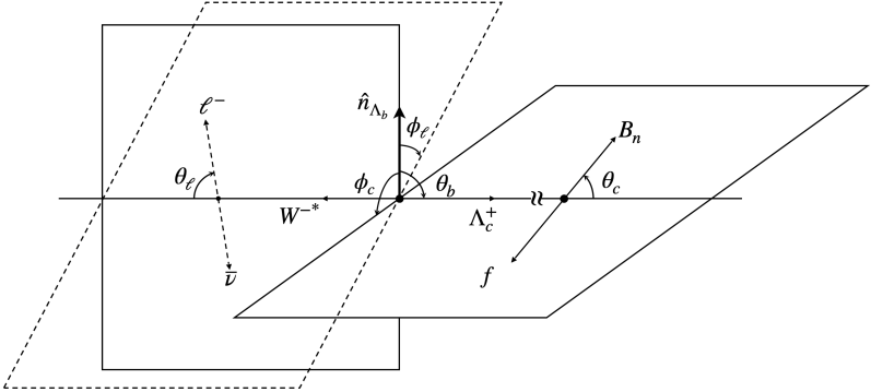
Figure 1: Definitions of the angles, where $B_{n}$ represents the daughter baryon and $f$ the rest of the decay particles.

We expand the angular distributions as

$$\begin{aligned} &\frac{\partial^{6}\Gamma(\Lambda_{b}\to\Lambda_{c}(\to B_{n}f)\ell^{-}\overline{\nu})}{\partial q^{2}\partial\vec{\Omega}}=\\ &\quad\quad{\cal B}(\Lambda_{c}\to B_{n}f)\frac{\zeta(q^{2})}{32\pi^{2}}\sum_{i=1}^{26}\text{Re}\left({\cal X}_{i}(a_{\pm},b_{\pm},t_{\pm}){\cal D}_{i}(\vec{\Omega})\right){\cal P}_{i}(\alpha,P_{b}),\end{aligned}$$ (14)

where $\alpha$ are the up-down asymmetries of $\Lambda_{c}\to B_{n}f$, $\vec{\Omega}=(\theta_{b,c,\ell}\,,\phi_{c,\ell})$, and explicit forms of ${\cal X}_{i}$, ${\cal P}_{i}$ and ${\cal D}_{i}$ can be found in Table 1, where we have taken the abbreviations:

$$a_{\pm}=H_{\pm\frac{1}{2},0}\,,~{}~{}~{}b_{\pm}=H_{\mp\frac{1}{2},\mp 1}\,,~{}~{}~{}t_{\pm}=H_{\pm\frac{1}{2},t}\,,~{}~{}~{}|\xi^{2}|=|\xi_{+}^{2}|+|\xi_{-}^{2}|\,,~{}~{}~{}|\xi_{\Delta}^{2}|=|\xi_{+}^{2}|-|\xi_{-}^{2}|\,,$$ (15)

with $\xi=a,b,t$ and $P_{2}=(3\cos^{2}\theta_{\ell}-1)/2$. The real-valued function in Eq. (14) guarantees that the partial decay widths are real. For an illustration, we have

$$\text{Re}\left({\cal X}_{7}{\cal D}_{7}\right)=\frac{3}{\sqrt{2}}\left[\text{Re}\left(2\delta_{\ell}(t_{-}b_{+}^{*}-b_{-}t_{+}^{*})+(a_{-}b_{+}^{*}+b_{-}a_{+}^{*})\right)\cos\phi_{\ell}\sin\theta_{b}\sin\theta_{\ell}-\right.$$

$$\quad\quad\quad\left.{\bf\text{Im}}\left(2\delta_{\ell}(t_{-}b_{+}^{*}-b_{-}t_{+}^{*})+(a_{-}b_{+}^{*}+b_{-}a_{+}^{*})\right)\sin\phi_{\ell}\sin\theta_{b}\sin\theta_{\ell}\right]\,,$$ (16)

$$\text{Re}\left({\cal X}_{12}{\cal D}_{12}\right)=\frac{3}{\sqrt{2}}\left[\text{Re}\left(2\delta_{\ell}(b_{-}t_{-}^{*}-t_{+}b_{+}^{*})-(a_{+}b_{+}^{*}+b_{-}a_{-}^{*})\right)\cos(\phi_{\ell}+\phi_{c})\sin\theta_{c}\cos\theta_{c}\right.$$

$$\quad\quad\quad-\left.{\bf\text{Im}}\left(2\delta_{\ell}(b_{-}t_{-}^{*}-t_{+}b_{+}^{*})-(a_{+}b_{+}^{*}+b_{-}a_{-}^{*})\right)\sin(\phi_{\ell}+\phi_{c})\sin\theta_{c}\cos\theta_{c}\right]\,,$$ (17)

by the identity of $\text{Re}({\cal X}_{i}{\cal D}_{i})=\text{Re}({\cal X}_{i})\text{Re}({\cal D}_{i})-{\bf\text{Im}}({\cal X}_{i}){\bf\text{Im}}({\cal D}_{i})$. For those ${\cal D}_{i}$, which are independent of $\phi_{c,\ell}$, we simply have Re$({\cal X}_{i}{\cal D}_{i})={\cal X}_{i}{\cal D}_{i}$. Notice that $\xi_{\pm}$ are real in the SM, and any observations of nonzero ${\bf\text{Im}}({\cal X}_{i})$ would be a smoking gun of NP. The angular distributions of $\overline{\Lambda_{b}}\to\overline{\Lambda_{c}}(\to\overline{B_{n}}\bar{f})\ell^{+}\nu$ can be obtained directly by taking $\theta_{\ell}\to\pi-\theta_{\ell}$ and $\alpha\to-\alpha$. In practice, $\delta_{l}$ can be taken as zero as an excellent approximation in the SM, with which $t_{\pm}$ can be neglected as well since they are always followed by $\delta_{\ell}$.

It is interesting to point out that, under the parity transformation, the helicity amplitudes behave differently as

$$a_{\pm}\to a_{\mp}\,,~{}~{}~{}b_{\pm}\to b_{\mp}\,,~{}~{}~{}t_{\pm}\to-t_{\mp}\,,$$ (18)

so that Re$({\cal X}_{7,12})$ and Im$({\cal X}_{7,12})$ are parity even and odd, respectively. If $\Lambda_{b}$ is unpolarized ($P_{b}=0$), it is clear that $\phi_{c}$ and $\phi_{\ell}$ can not be measured separately. In this case, it is convenient to introduce a new set of azimuthal coordinates as

$$\Phi=\phi_{\ell}+\phi_{c}\,,\,\,\,\,\,\,\,\,\, 0<\Phi<2\pi\,,$$ (19)

$$\Phi_{\Delta}=\frac{1}{2}(\phi_{\ell}-\phi_{c})\,,\,\,\,\,\,\, -\pi<\Phi_{\Delta}<\pi\,.$$

To obtain the unpolarized angular distributions from the polarized ones, one can integrate over $\Phi_{\Delta}$ and $\cos\theta_{b}$, in which ${\cal D}_{4\text{--}8,14\text{--}26}$ are zero. As a cross-check, we find that the results are identical to those given in Ref. Korner .

Table 1: The angular distributions of $\Lambda_{b}\to\Lambda_{c}(\to B_{n}f)\ell^{-}\overline{\nu}$ with $P_{2}=(3\cos^{2}\theta_{\ell}-1)/2$ and the parameters of $a$, $b$ and $t$ defined in Eq. (15).

$i$	${\cal X}_{i}$	$P_{i}$	${\cal D}_{i}$
1	$(\delta_{\ell}+1)(|a|^{2}+|b|^{2})+3\delta_{\ell}|t|^{2}$	$1$	$1$
2	$(2\delta_{\ell}-1)(|a|^{2}-\frac{1}{2}|b|^{2})$	$1$	$P_{2}$
3	$-6\delta_{\ell}\left(\text{Re}\left(a_{+}t_{+}^{*}\right)+\text{Re}\left(a_{-}t_{-}^{*}\right)\right)+\frac{3}{2}|b_{\Delta}|^{2}$	$1$	$\cos\theta_{\ell}$
4	$(\delta_{\ell}+1)(|a_{\Delta}|^{2}+|b_{\Delta}|^{2})+3\delta_{\ell}|t_{\Delta}|^{2}$	$P_{b}$	$\cos\theta_{b}$
5	$(2\delta_{\ell}-1)(|a_{\Delta}|^{2}-\frac{1}{2}|b_{\Delta}|^{2})$	$P_{b}$	$\cos\theta_{b}P_{2}$
6	$-6\delta_{\ell}\left[\text{Re}(a_{+}t_{+}^{*})-\text{Re}(a_{-}t_{-}^{*})\right]-\frac{3}{2}|b_{\Delta}|^{2}$	$P_{b}$	$\cos\theta_{b}\cos\theta_{\ell}$
7	$\frac{3}{\sqrt{2}}\left[2\delta_{\ell}(t_{-}b_{+}^{*}-b_{-}t_{+}^{*})+(a_{-}b_{+}^{*}+b_{-}a_{+}^{*})\right]$	$P_{b}$	$e^{i\phi_{\ell}}\sin\theta_{b}\sin\theta_{\ell}$
8	$\frac{3}{\sqrt{2}}(2\delta_{\ell}-1)(b_{-}a_{+}^{*}-a_{-}b_{+}^{*})$	$P_{b}$	$e^{i\phi_{\ell}}\sin\theta_{b}\sin\theta_{\ell}\cos\theta_{\ell}$
9	$(\delta_{\ell}+1)(|a_{\Delta}|^{2}-|b_{\Delta}|^{2})+3\delta_{\ell}|t_{\Delta}|^{2}$	$\alpha$	$\cos\theta_{c}$
10	$(2\delta_{\ell}-1)(|a_{\Delta}|^{2}+\frac{1}{2}|b_{\Delta}|^{2})$	$\alpha$	$\cos\theta_{c}P_{2}$
11	$6\delta_{\ell}\left(\text{Re}\left(a_{-}t_{-}^{*}\right)-\text{Re}\left(a_{+}t_{+}^{*}\right)\right)-\frac{3}{2}|b|^{2}$	$\alpha$	$\cos\theta_{c}\cos\theta_{\ell}$
12	$\frac{3}{\sqrt{2}}\left[2\delta_{\ell}(b_{-}t_{-}^{*}-t_{+}b_{+}^{*})-(a_{+}b_{+}^{*}+b_{-}a_{-}^{*})\right]$	$\alpha$	$e^{i\Phi}\sin\theta_{c}\cos\theta_{c}$
13	$\frac{3}{\sqrt{2}}\left[2\delta_{\ell}(a_{+}b_{+}^{*}-b_{-}a_{-}^{*})+(b_{-}a_{-}^{*}-a_{+}b_{+}^{*})\right]$	$\alpha$	$e^{i\Phi}\sin\theta_{c}\cos\theta_{c}\cos\theta_{\ell}$
14	$(2\delta_{\ell}+1)a_{+}a_{-}^{*}$	$P_{b}\alpha$	$\sin\theta_{b}\sin\theta_{c}P_{2}$
15	$2\delta_{\ell}(|a|^{2}+|b|^{2})-(|a|^{2}+1/2|b|^{2})$	$P_{b}\alpha$	$\cos\theta_{b}\cos\theta_{c}P_{2}$
16	$\delta_{\ell}(|a|^{2}-|b|^{2}+3|t|^{2})+(|a|^{2}-|b|^{2})$	$P_{b}\alpha$	$\cos\theta_{b}\cos\theta_{c}$
17	$-6\delta_{\ell}\left(\text{Re}(a_{+}t_{+}^{*})+\text{Re}(a_{-}t_{-}^{*})\right)-\frac{3}{2}|b_{\Delta}|^{2}$	$P_{b}\alpha$	$\cos\theta_{b}\cos\theta_{c}\cos\theta_{\ell}$
18	$(2-4\delta_{\ell})a_{-}a_{+}^{*}$	$P_{b}\alpha$	$e^{-i\phi_{c}}\sin\theta_{b}\sin\theta_{c}P_{2}$
19	$(1-2\delta_{\ell})b_{-}b_{+}^{*}$	$P_{b}\alpha$	$e^{i(\phi_{c}+2\phi_{\ell})}\sin\theta_{b}\sin\theta_{c}P_{2}$
20	$-2\delta_{\ell}(a_{+}a_{-}^{*}+3t_{+}t_{-}^{*})-2a_{+}a_{-}^{*}$	$P_{b}\alpha$	$e^{i\phi_{c}}\sin\theta_{b}\sin\theta_{c}$
21	$(2\delta_{\ell}-1)b_{-}b_{+}^{*}$	$P_{b}\alpha$	$e^{i(\phi_{c}+2\phi_{\ell})}\sin\theta_{b}\sin\theta_{c}$
22	$6\delta_{\ell}(a_{+}t_{-}^{*}+t_{+}a_{-}^{*})$	$P_{b}\alpha$	$e^{i\phi_{c}}\sin\theta_{b}\sin\theta_{c}\cos\theta_{\ell}$
23	$\frac{3}{\sqrt{2}}\left[(b_{-}a_{+}^{*}-a_{-}b_{+}^{*})-2\delta_{\ell}(b_{-}t_{+}^{*}+t_{-}b_{+}^{*})\right]$	$P_{b}\alpha$	$e^{i\phi_{\ell}}\sin\theta_{b}\sin\theta_{\ell}\cos\theta_{c}$
24	$\frac{3}{\sqrt{2}}\left[(b_{-}a_{-}^{*}-a_{+}b_{+}^{*})-2\delta_{\ell}(b_{-}t_{-}^{*}+t_{+}b_{+}^{*})\right]$	$P_{b}\alpha$	$e^{i\Phi}\sin\theta_{c}\sin\theta_{\ell}\cos\theta_{b}$
25	$\frac{3}{\sqrt{2}}\left[2\delta_{\ell}(a_{-}b_{+}^{*}+b_{-}a_{+}^{*})-(a_{-}b_{+}^{*}+b_{-}a_{+}^{*})\right]$	$P_{b}\alpha$	$e^{i\phi_{\ell}}\sin\theta_{b}\sin\theta_{\ell}\cos\theta_{c}\cos\theta_{\ell}$
26	$\frac{3}{\sqrt{2}}\left[2\delta_{\ell}(b_{-}a_{-}^{*}-a_{+}b_{+}^{*})-(a_{+}b_{+}^{*}+b_{-}a_{-}^{*})\right]$	$P_{b}\alpha$	$e^{i\Phi}\sin\theta_{c}\sin\theta_{\ell}\cos\theta_{b}\cos\theta_{\ell}$

With Table 1, one can construct several observables in a model independent way. The simplest ones would be the partial and total decay widths, read as

$$\frac{d\Gamma(\Lambda_{b}\to\Lambda_{c}\ell^{-}\overline{\nu})}{dq^{2}}=\zeta(q^{2}){\cal X}_{1}\,,$$ (20)

and

$$\Gamma=\Gamma(\Lambda_{b}\to\Lambda_{c}\ell^{-}\overline{\nu})=\int^{(M_{b}-M_{c})^{2}}_{m_{\ell}^{2}}\zeta(q^{2}){\cal X}_{1}dq^{2}\,,$$ (21)

respectively. It shall be clear that $\Gamma$ is independent of $\Lambda_{c}\to B_{n}f$. Likewise, there are several observables that can be defined independent of $\Lambda_{c}\to B_{n}f$, and it is reasonable to measure them separately as they do not suffer from the smallness of ${\cal B}(\Lambda_{c}\to B_{n}f)$. In fact, the angular distributions without cascade decays can be obtained straightforwardly by integrating over $(\cos\theta_{c},\phi_{c})$, resulting in

$$\begin{aligned} \frac{\partial^{4}\Gamma(\Lambda_{b}\to\Lambda_{c}\ell^{-}\overline{\nu})}{\partial q^{2}\partial\cos\theta_{b}\cos\theta_{\ell}\partial\phi_{\ell}}=\frac{\zeta(q^{2})}{8\pi}\sum_{i=1}^{8}\text{Re}\left({\cal X}_{i}(a_{\pm},b_{\pm},t_{\pm}){\cal D}_{i}(\vec{\Omega})\right){\cal P}_{i}(0,P_{b})\,,\end{aligned}$$ (22)

which is clearly independent of $\alpha$. As a cross-check, we find that Eq. (22) reduces to the ones given by Ref. KornerNeutron with an appropriate substitution.

There are some quantities that deserve a closer look. The forward-backward asymmetries for $W^{-*}\to l^{-}\overline{\nu}$ and $\Lambda_{c}\to B_{n}f$ are defined as

$$A_{FB}=2\left(\int^{1}_{0}-\int^{0}_{-1}\right)\Gamma_{\cos\theta_{\ell}}d\cos\theta_{\ell}=\frac{1}{\Gamma}\int^{(M_{b}-M_{c})^{2}}_{m_{\ell}^{2}}\zeta(q^{2}){\cal X}_{3}dq^{2}\,,$$

$$A_{PL}=\frac{2}{\alpha}\left(\int^{1}_{0}-\int^{0}_{-1}\right)\Gamma_{\cos\theta_{c}}d\cos\theta_{c}=\frac{1}{\Gamma}\int^{(M_{b}-M_{c})^{2}}_{m_{\ell}^{2}}\zeta(q^{2}){\cal X}_{9}dq^{2}\,,$$ (23)

where we have adopted the shorthand notation,

$$\Gamma_{\vec{\Omega}}=\frac{1}{{\cal B}(\Lambda_{c}\to B_{n}f)}\frac{1}{\Gamma}\frac{\partial\Gamma(\Lambda_{b}\to\Lambda_{c}(\to B_{n}f)\ell^{-}\overline{\nu})}{\partial{\vec{\Omega}}}\,.$$ (24)

The up-down asymmetries $A_{UD}$, on the other hand, are given by

$$A_{UD}=\frac{2}{P_{b}}\left(\int^{1}_{0}-\int^{0}_{-1}\right)\Gamma_{\cos\theta_{b}}d\cos\theta_{b}=\frac{1}{\Gamma}\int^{(M_{b}-M_{c})^{2}}_{m_{\ell}^{2}}\zeta(q^{2}){\cal X}_{4}dq^{2}\,,$$ (25)

which require $P_{b}\neq 0$ for an experimental measurement.

Here, it is an appropriate place to revisit $A_{\lambda}^{c}$ in Eq. (II) explicitly. We have

$$\left|A_{\pm\frac{1}{2}}^{c}\right|^{2}=\frac{1}{2}\left(1\pm\alpha\right)\,,$$ (26)

where $\alpha$ are the up-down asymmetries of $\Lambda_{c}\to B_{n}f$, with the experimental values given by pdg

$$\begin{aligned} \alpha(\Lambda_{c}\to\Lambda\pi^{+},&\Sigma^{0}\pi^{+},\Sigma^{+}\pi^{0},pK^{0}_{s})=\\ &(-0.84\pm 0.09,-0.55\pm 0.11,-0.73\pm 0.18,0.2\pm 0.5),\end{aligned}$$ (27)

Similarly, for the three-body $\Lambda_{c}$ decays, we have $\alpha=A_{UD}^{c}$, where $A_{UD}^{c}$ are defined by substituting $\Lambda_{c}\to B_{n}f$ for $\Lambda_{b}\to\Lambda_{c}\ell^{-}\overline{\nu}$ in Eq. (25). In particular, $\alpha$ are found to be

$$\alpha(\Lambda_{c}\to pK^{-}\pi^{+},\Lambda l^{+}\nu)=(0.89\pm 0.10,-0.32),$$ (28)

from the $SU(3)_{F}$ analysis UP-down and light-front quark model lightfront , respectively.

The azimuthal angles are closely related to the triple product asymmetries, which flip signs under TR transformation TimeReversal . To probe them, we define

$${\cal T}_{\ell}=\frac{1}{P_{b}}\left(\int^{\pi}_{0}-\int_{\pi}^{2\pi}\right)\Gamma_{\phi_{\ell}}d\phi_{\ell}=-\frac{\pi^{2}}{8\Gamma}\int^{(M_{b}-M_{c})^{2}}_{m_{\ell}^{2}}\zeta(q^{2}){\bf\text{Im}}({\cal X}_{7})dq^{2}\,,$$ (29)

$${\cal T}_{c}=\frac{1}{\alpha}\left[\left(\int^{\pi}_{0}-\int_{\pi}^{2\pi}\right)d\Phi\right]\left[\left(\int_{0}^{1}-\int^{0}_{-1}\right)d\cos\theta_{c}\right]\Gamma_{\phi_{\ell},\cos\theta_{c}}$$

$$\quad=-\frac{2}{3\pi\Gamma}\int^{(M_{b}-M_{c})^{2}}_{m_{\ell}^{2}}\zeta(q^{2}){\bf\text{Im}}({\cal X}_{12})dq^{2}\,,$$

which are proportional to the complex phases of $\xi_{\pm}$, and vanish without NP. Comparing to the direct CP asymmetries, TR asymmetries do not require strong phases, which are great advantages to probe CP violation as strong phases are absent in the semileptonic decays. Note that one can also construct other TR asymmetries from ${\cal X}_{8,13,18\text{--}26}$.

III Contributions from possible new physics

Let us consider the dimension-six effective Hamiltonian from NP with left-handed neutrinos, read as where $P_{R,L}=(1\pm\gamma_{5})$, $C_{S,P,R,L,T}$ are the Wilson coefficients, which are complex and depend on the lepton flavors in general, and $N$ in the superscript indicates that NP is considered. The effects of $C_{S,P,R,L}$ can be absorbed by redefining the amplitudes as

$$a_{\pm}^{N}=\left(1+C_{L}\right)a_{\pm}+C_{R}a_{\mp}\,,~{}~{}~{}b^{N}_{\pm}=\left(1+C_{L}\right)b_{\pm}+C_{R}b_{\mp}\,,$$

$$t_{\pm}^{N}=\left(1+C_{L}\right)t_{\pm}+C_{R}t_{\mp}-\frac{\sqrt{Q_{+}q^{2}}}{m_{\ell}}C_{S}f_{s}\pm\frac{\sqrt{Q_{-}q^{2}}}{m_{\ell}}C_{P}g_{p}\,,$$ (30)

where $f_{s}$ and $g_{p}$ are defined by

$$\langle\Lambda_{c}|\overline{c}\left(1+\gamma_{5}\right)b|\Lambda_{b}\rangle=\overline{u}_{c}\left(f_{s}+g_{p}\gamma_{5}\right)u_{b}\,.$$ (31)

The derivations can be found in Appendix B. Note that in Eq. (III), $\xi_{\pm}$ are calculated within the SM given in Eq. (II). The angular distributions can be easily obtained by substituting $\xi_{\pm}^{N}$ for $\xi_{\pm}$ in Table 1 . In the case of $C_{R,S,P}=0$, the effect of $C_{L}$ can be absorbed by redefining $V_{cb}$ as $V_{cb}(1+C_{L})$, leaving the angular distributions unaltered. Therefore, in the following, we would simply take $C_{L}=0$.

Let us first consider the case that $C_{R}\neq 0$ with $C_{S,P}=0$. For the total decay widths, $C_{R}$ would be polluted by the uncertainties of the form factors. However, we can utilize that $\xi_{\pm}$ are real, whereas $C_{R}$ can be complex in general. Plugging Eq. (III) in Eq. (II), we arrive at

$${\bf\text{Im}}\left({\cal X}_{7}^{N}\right)=3\sqrt{2}\,{\bf\text{Im}}(C_{R})\left(a_{+}b_{+}-a_{-}b_{-}\right)\,,$$

$${\bf\text{Im}}\left({\cal X}_{12}^{N}\right)=3\sqrt{2}\,{\bf\text{Im}}(C_{R})\left(a_{+}b_{-}-a_{-}b_{+}\right)\,,$$ (32)

where we have taken $\xi_{\pm}$ as real, calculated by Eq. (II).

On the other hand, the effects of $C_{S,P}$ are largely enhanced by the smallness of the lepton quark masses when $q^{2}/m_{\ell}^{2}\gg 1$. Therefore, measuring $t_{\pm}$ in high $q^{2}$ regions would be useful to constrain the values of $C_{S,P}$. To diminish the uncertainties from the form factors, one can examine the complex phases, given by

$${\bf\text{Im}}\left({\cal X}_{7}^{N}\right)=\frac{3}{\sqrt{2}}m_{\ell}\left[-{\bf\text{Im}}(C_{S})\sqrt{\frac{Q_{+}}{q^{2}}}f_{s}\left(b_{+}+b_{-}\right)+{\bf\text{Im}}(C_{P})\sqrt{\frac{Q_{-}}{q^{2}}}g_{p}\left(b_{-}-b_{+}\right)\right]\,,$$

$${\bf\text{Im}}\left({\cal X}_{12}^{N}\right)=\frac{3}{\sqrt{2}}m_{\ell}\left[{\bf\text{Im}}(C_{S})\sqrt{\frac{Q_{+}}{q^{2}}}f_{s}\left(b_{+}+b_{-}\right)+{\bf\text{Im}}(C_{P})\sqrt{\frac{Q_{-}}{q^{2}}}g_{p}\left(b_{-}-b_{+}\right)\right]\,,$$ (33)

where we have taken $C_{R}=0$. By collecting Eqs. (III) and (III), the net effects of NP on ${\cal T}_{\ell,c}$ are summarized as follows

$$\mathcal{T}_{\ell} = -\frac{3\pi^{2}}{8\sqrt{2}}\left(\operatorname{Im}\left(C_{R}\right)\mathcal{Y}_{R}-\operatorname{Im}\left(C_{S}\right)\mathcal{Y}_{S}+\operatorname{Im}\left(C_{P}\right)\mathcal{Y}_{P}\right)$$

$${\cal T}_{c} = -\frac{\sqrt{2}}{\pi}\left({\bf\text{Im}}(C_{R}){\cal Y}^{\prime}_{R}+{\bf\text{Im}}(C_{S}){\cal Y}_{S}+{\bf\text{Im}}(C_{P}){\cal Y}_{P}\right)\,,$$ (34)

where

$${\cal Y}_{R}^{(\prime)} = \frac{1}{\Gamma}\int^{(M_{b}-M_{c})^{2}}_{m_{\ell}^{2}}2\zeta\left(a_{+}b_{+(-)}-a_{-}b_{-(+)}\right)dq^{2}\,,$$

$${\cal Y}_{S} = \frac{1}{\Gamma}\int^{(M_{b}-M_{c})^{2}}_{m_{\ell}^{2}}\zeta m_{\ell}\sqrt{\frac{Q_{+}}{q^{2}}}f_{s}\left(b_{+}+b_{-}\right)dq^{2}\,,$$

$${\cal Y}_{P} = \frac{1}{\Gamma}\int^{(M_{b}-M_{c})^{2}}_{m_{\ell}^{2}}\zeta m_{\ell}\sqrt{\frac{Q_{+}}{q^{2}}}g_{p}\left(b_{-}-b_{+}\right)dq^{2}\,.$$ (35)

Notice that $\Gamma$ also depends on $C_{R,S,P}$. However, in this work, we take $C_{R,S,P}$ as zero in $\Gamma$ as a first order approximation, and therefore ${\cal Y}^{(\prime)}_{R,S,P}$ can be computed once the form factors are given.

To examine TR asymmetries in the experiments, we define

$$\Delta N_{\ell}\equiv N(\pi>\phi_{\ell}>0)-N(2\pi>\phi_{\ell}>\pi)=\epsilon N_{\Lambda_{b}}{\cal T}_{\ell}{\cal B}(\Lambda_{b}\to\Lambda_{c}^{+}\ell^{-}\nu)P_{b}\,,$$

$$\Delta N_{f}\equiv N(\pi>\phi_{c}>0,\cos\theta_{c}>0)+N(2\pi>\phi_{c}>\pi,\cos\theta_{c}<0)$$

$$~{}~{}~{}~{}-N(\pi>\phi_{c}>0,\cos\theta_{c}<0)-N(2\pi>\phi_{c}>\pi,\cos\theta_{c}>0)$$

$$= \epsilon N_{\Lambda_{b}}{\cal T}_{c}{\cal B}(\Lambda_{b}\to\Lambda_{c}^{+}\ell^{-}\nu){\cal B}(\Lambda_{c}\to B_{n}f)\alpha(\Lambda_{c}\to B_{n}f)\,,$$ (36)

which hold at ${N\to\infty}$ with $N$ the number of the observed events, where $N_{\Lambda_{b}}$ is the numbers of $\Lambda_{b}$ in experiments, and $\epsilon$ is the efficiency for the experimental reconstruction. To reduce the statistical uncertainties in $\Delta N_{f}$, we can sum over the decay modes of $\Lambda_{c}^{+}$, given as

$$\Delta N_{c}=\sum_{f}\left|N_{f}\right|=\epsilon N_{\Lambda_{b}}{\cal T}_{c}{\cal B}(\Lambda_{b}\to\Lambda_{c}^{+}\ell^{-}\nu)\sum_{B_{n}f}\left|{\cal B}(\Lambda_{c}\to B_{n}f)\alpha(\Lambda_{c}\to B_{n}f)\right|\,.$$ (37)

As $\Delta N_{{\ell,c}}$ are proportional to ${\cal T}_{\ell,c}$, a nonzero value of $\Delta N_{{\ell}}$ or $\Delta N_{{c}}$ would be a smoking gun of NP.

The full angular distributions including the tensor operator are given in Appendix C. For simplicity, we take $C_{T}=0$ in the numerical analysis, as they can not be reduced to the form of Eq. (6), which breaks the angular analysis. In addition, the tensor operator is closely related to the scalar ones by the Fierz transformation in the leptoquark effective field theory Leptoquark .

IV Numerical results

As mentioned in Sec. III, nonzero signals of ${\cal T}_{\ell,c}$ can be clear evidence of CP violation from NP with $t^{N}_{\pm}$ largely enhanced in high $q^{2}$ regions by $C_{S,P}$. In Eq. (III), ${\bf\text{Im}}(C_{R,S,P})$ are in general free parameters of NP, whereas ${\cal Y}_{R,S,P}^{(\prime)}$ can be computed by the form factors. In this work, we utilize the homogeneous bag model to estimate the form factors Liu:2022pdk , which agree well with those by the lattice QCD calculation as well as the heavy quark symmetry lattice .

The values of ${\cal Y}_{R,S,P}^{(\prime)}$ are listed in Table 2, from which one can see that ${\cal Y}_{R}$ and ${\cal Y}_{R}^{\prime}$ are both sizable for all flavors, giving us a good opportunity to examine Im$(C_{R})$. In contrast, the values of ${\cal Y}_{S,P}$ for $\ell=e$ and $\mu$ are suppressed due to $m_{\ell}$. For $\ell=\tau$, ${\cal Y}_{S,P}$ are still 3 times smaller than ${\cal Y}_{R}^{(\prime)}$. Hence, Im$(C_{S,P})$ are much more difficult to be observed in the experiments comparing to Im$(C_{R})$.

Table 2: Parameters defined in Eq. (III), where the uncertainties come from the model calculation.

$\ell$	${\cal Y}_{R}$	${\cal Y}_{R}^{\prime}$	${\cal Y}_{S}$	${\cal Y}_{P}$
$e$	$-0.238(11)$	$0.703(13)$	$<10^{-4}$	$<10^{-4}$
$\mu$	$-0.237(12)$	$0.701(13)$	$-0.0037(2)$	$0.0136(2)$
$\tau$	$-0.149(6)$	$0.438(8)$	$-0.039(2)$	$0.180(2)$

To explain the excesses of $R_{D^{(*)}}$, $C_{R,S,P}$ are found to be tiny for $\ell=e$ and $\mu$, but fortunately, $C_{R}=\pm 0.42(7)i$ is huge for $\ell=\tau$ Leptoquark . We have plotted $\zeta(\partial{\cal Y}_{R}^{(\prime)}/\partial q^{2})$ for $\ell=\tau$ in FIG. 2, where the bands represent the uncertainties from the form factors. One can see that the ideal $q^{2}$ region to search for the asymmetries lies around $7$ GeV${}^{2}<q^{2}<9$ GeV², since they are huge within the region. Finally, putting the values of ${\cal Y}_{R}^{(\prime)}$ and $C_{R}=\pm 0.42(7)i$ in Eq. (III), we find that

$${\cal T}_{\ell}=\pm 0.16(3)\,,~{}~{}~{}~{}{\cal T}_{c}=\pm 0.08(2)\,,$$ (42)

for $\Lambda_{b}\to\Lambda_{c}\tau^{-}\overline{\nu}$. Notice that the signs are irrelevant for searching evidence of NP as long as they are nonzero. To estimate the results at LHCb run2, we take $N_{\Lambda_{b}}=5\times 10^{9}$, $P_{b}=0.03$, $\varepsilon=10^{-4}$, and

$$\sum_{f}\left|{\cal B}(\Lambda_{c}\to B_{n}f)\alpha(\Lambda_{c}\to B_{n}f)\right|=6\times 10^{-2}\,,$$ (43)

resulting in that $|\Delta N_{\ell}|\approx 50$ and $\Delta N_{c}\approx 20$ for $\ell=\tau$, which are large and ready to be measured. Here, Eq. (43) is derived by crunching up the numbers in Eqs. (27) and (28).

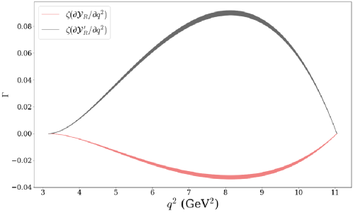
Figure 2: $q^{2}$ dependence of $\zeta(\partial{\cal Y}_{R}^{(\prime)}/\partial q^{2})$ in $\Lambda_{b}\to\Lambda_{c}\tau^{-}\overline{\nu}$, where the bands represent the uncertainties caused by the form factors.

To probe the effects of the scalar operators, we find that ${\cal X}_{6}$, which can be understood as a combination of $A_{FB}$ and $A_{UD}$, is sensitive to $C_{S,P}$ for $\ell=\tau$. The results are plotted in FIG. 3, where we have taken $C_{P}=C_{S}$. In the region of 9 GeV${}^{2}<q^{2}<$10 GeV², ${\cal X}_{6}$ can be enhanced largely. In particular, it is twice larger with $C_{S}=0.2$ in comparison to that in the SM.

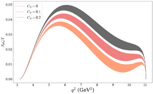
Figure 3: $q^{2}$ dependence of ${\cal X}_{6}\zeta/\Gamma$ with $\ell=\tau$ for $C_{S}=0,0.1$ and $0.2$, respectively.

V Summary

Based on the helicity formalism, we have given the full angular distributions of $\Lambda_{b}\to\Lambda_{c}(\to B_{n}f)\ell^{-}\overline{\nu}$. In particular, we have identified TR violating terms, which vanish in the SM due to the lack of relative complex phases. Since strong phases are not required in these TR violating observables in contrast to the direct CP asymmetries, they can be reliably calculated. The angular distributions have been given explicitly with the helicity amplitudes in Table 1. We have cross-checked our results with those in Refs. Korner ; KornerNeutron , and found that they are consistent. Note that our results can be easily applied to $\Xi_{b}\to\Xi_{c}(\to B_{n}f)\ell^{-}\overline{\nu}$ with trivial modifications.

Notably, the effects of NP can be absorbed by redefining the helicity amplitudes as demonstrated in Eq. (III) with $\xi_{\pm}$ calculated in the SM. We recommend the experiments to measure the TR violating observables of ${\cal T}_{\ell,c}$ defined in Eq. (29) for searching NP as they vanish in the SM. To compare with the experiments, $\Delta N_{\ell,c}$ have been defined by the numbers of the observed events, which are proportional to ${\cal T}_{\ell,c}$. Based on $C_{R}=\pm 0.42(7)i$ for $\ell=\tau$, we have obtained that $|\Delta N_{\ell,c}|\approx 50,20$ at LHCb run2, which are sufficient for measurements. On the other hand, we have pointed out that ${\cal X}_{6}$ is sensitive to $C_{S,P}$ for $\Lambda_{b}\to\Lambda_{c}\tau^{-}\overline{\nu}$, which can be largely enhanced in the high $q^{2}$ region.

Appendix A Dirac spinors

In this work, we choose fermions and antifermions in $p\hat{z}$ and $-p\hat{z}$ directions, respectively. We have that

$$u_{+}=\left(\begin{array}[]{c}E_{+}\\ 0\\ E_{-}\\ 0\end{array}\right)\,,\quad u_{-}=\left(\begin{array}[]{c}0\\ E_{+}\\ 0\\ -E_{-}\end{array}\right)\,,\quad v_{+}=\left(\begin{array}[]{c}E_{-}\\ 0\\ -E_{+}\\ 0\end{array}\right)\,,\quad v_{-}=\left(\begin{array}[]{c}0\\ -E_{-}\\ 0\\ -E_{+}\end{array}\right)\,,$$ (60)

with $``\pm"$ denoting the helicities, $E_{\pm}=\sqrt{E\pm m}$, and $m$ the particle mass. Notice that the relative signs are crucial, fixed by the relations

$$u_{-}=L^{u}_{z}R_{y}(\pi)(L_{z}^{u})^{-1}u_{+}\,,~{}~{}~{}v_{-}=(L_{z}^{v})^{-1}R_{y}(\pi)L_{z}^{v}v_{+}\,,$$ (61)

where $R_{y}$ is the rotation matrix toward $\hat{y}$, and $L_{z}^{u,v}$ are the Lorentz boost operators toward $\hat{z}$. Here, $L_{z}^{u,v}$ are taken in a way such that $L_{z}^{u-1}u_{\pm}$ and $L_{z}^{v}v_{\pm}$ are at rest.

Appendix B Angular distributions in the standard model

We now sketch the derivation of Eq. (II). We start with a two-body decay of $i\to f_{1}f_{2}$, where $i$ and $f_{1,2}$ are unspecific particles. The decay distribution is given as

$$\frac{\partial^{2}\Gamma(i\to f_{1}f_{2})}{\partial\phi\partial\cos\theta}\propto\sum_{\lambda_{1},\lambda_{2}}\left|\langle p,\theta,\phi,\lambda_{1},\lambda_{2}|U(\infty,-\infty)|i;J,J_{z}\rangle\right|^{2}\,,$$ (62)

$$|p,\theta,\phi,\lambda_{1},\lambda_{2}\rangle=R_{z}(\phi)R_{y}(\theta)\left(|f_{1};\vec{p}=p\vec{z},\lambda_{1}\rangle\otimes|f_{2};\vec{p}=-p\vec{z},\lambda_{2}\rangle\right)\,,$$ (63)

where $U$ is the time evolution operator, $J$ and $J_{z}$ are the angular momentum and its $z$ component of the initial particle, $R_{y,z}$ are the rotational operators pointing toward $(y,z)$, and $\lambda_{1,2}$ are the helicities of $f_{1,2}$. In the decay distributions, we have to sum over the helicities of the outgoing particles as they are difficult to be probed in the experiments.

In two-body systems, states with definite angular momenta and helicities can be constructed as

$$|\lambda_{1}\,,\lambda_{2},J,J_{z}\rangle=\frac{1}{(2J+1)\pi}\int d\cos\theta d\phi|p,\theta,\phi,\lambda_{1}\,,\lambda_{2}\rangle e^{iJ_{z}\phi}d^{J}(\theta)^{J_{z}}\,_{\lambda_{1}-\lambda_{2}}\,,$$ (64)

along with the identity

$$1=\sum_{J,J_{z}}\frac{4\pi}{2J+1}|J,J_{z},\lambda_{1},\lambda_{2}\rangle\langle J,J_{z},\lambda_{1},\lambda_{2}|.$$ (65)

Notice that in Eq. (64), $\lambda_{1,2}$ are unaltered because they are rotational scalars. By inserting Eq. (65) in Eq. (62), we obtain

$$\frac{\partial^{2}\Gamma(i\to f_{1}f_{2})}{\partial\phi\partial\cos\theta}\propto\sum_{\lambda_{1},\lambda_{2}}\left|e^{iJ_{z}\phi}d^{J}(\theta)^{J_{z}}\,_{\lambda_{1}-\lambda_{2}}H_{\lambda_{1}\lambda_{2}}\right|^{2}\,,$$ (66)

with

$$H_{\lambda_{1},\lambda_{2}}\equiv\langle J,J_{z},\lambda_{1},\lambda_{2}|U(\infty,-\infty)|i;J,J_{z}\rangle\,.$$ (67)

Clearly, $H_{\lambda_{1},\lambda_{2}}$ is independent of $J_{z}$ since $U$ must be a scalar. In Eq. (66), we see that the decay distributions are separated into two different parts. The kinematic part is described by the Wigner-d matrix whereas the dynamical part $H_{\lambda_{1},\lambda_{2}}$.

The three-body decay distributions can be obtained by decomposing the systems into a product of two-body decays as demonstrated in Eq. (6).

Appendix C Contributions from scalar and current operators

The contributions of $C_{L}$ are given by

$$\xi_{\pm}\to(1+C_{L})\xi_{\pm}\,,$$ (68)

due to the same coupling in the SM. Furthermore, those of $C_{R}$ can be obtained straightforwardly by

$$\xi_{\pm}\to\xi_{\pm}+C_{R}\xi_{\mp}\,,$$ (69)

as $\overline{c}\gamma^{\mu}P_{L,R}b$ are related by the parity.

The scalar operators contribute to the amplitudes as

$$\frac{G_{f}}{\sqrt{2}}V_{cb}L_{t}^{N}B_{t}^{N}\,,~{}~{}~{}L_{t}^{N}={\cal C}\overline{u}_{\ell}P_{L}v_{\nu}\,,~{}~{}~{}B_{t}^{N}={\cal C}^{-1}\overline{u}_{c}\left(C_{S}f_{s}+C_{P}g_{p}\gamma_{5}\right)u_{b}\,,$$ (70)

where ${\cal C}$ is a constant, Clearly, $B_{t}^{N}$ and $L_{t}^{N}$ can be viewed as the transitions of $\Lambda_{b}\to\Lambda_{c}P^{-}$ and $P^{-}\to l^{-}\overline{\nu}$, respectively, with $P^{-}$ an effective particle from NP. As $P^{-}$ is spinless, $L_{t}^{N}B_{t}^{N}$ is only related to $L_{t}B_{t}$ in Eq. (6). By adjusting ${\cal C}$ such that $L_{t}^{N}=L_{t}$, we arrive at

$$t_{\pm}^{N}=t_{\pm}-\frac{\sqrt{Q_{+}q^{2}}}{m_{\ell}}C_{S}f_{s}\pm\frac{\sqrt{Q_{-}q^{2}}}{m_{\ell}}C_{P}g_{p}\,.$$ (71)

By collecting Eqs. (68), (69) and (71), we obtain Eq. (III). It is interesting to see that all the contributions can be encapsulated in $\xi_{\pm}$, which already exist in the SM.

Appendix D Contributions from tensor operator

To cooperate the tensor operator with the helicity amplitudes, by utilizing Eq. (2) we decompose the products of the Minkowski metric as

$$\left(g^{\mu\nu}g^{\mu^{\prime}\nu^{\prime}}-g^{\mu^{\prime}\nu}g^{\mu\nu^{\prime}}\right)=\sum_{\lambda}\left(-V_{1}^{\mu\mu^{\prime}}(\lambda)V_{1}^{\nu\nu^{\prime}*}(\lambda)+V_{2}^{\mu\mu^{\prime}}(\lambda)V_{2}^{\nu\nu^{\prime}*}(\lambda)\right)\,,$$ (72)

with

$$V_{1}^{\mu\mu^{\prime}}(\lambda)=\left(\varepsilon_{t}^{\mu}\varepsilon^{\mu^{\prime}}_{\lambda}-\varepsilon_{t}^{\mu^{\prime}}\varepsilon^{\mu}_{\lambda}\right)\,,~{}~{}~{}V_{2}^{\mu\mu^{\prime}}(\lambda)=\frac{1}{\sqrt{2}}\left(\varepsilon_{\lambda_{1}}^{\mu}\varepsilon^{\mu^{\prime}}_{\lambda_{2}}-\varepsilon_{\lambda_{1}}^{\mu^{\prime}}\varepsilon^{\mu}_{\lambda_{2}}\right)\,,$$ (73)

and

$$(\lambda_{1},\lambda_{2})=(1,0),(1,-1),(0,-1)\,,~{}~{}\text{for}~{}~{}\lambda=1,0,-1\,.$$ (74)

To see that $V_{1,2}$ can be viewed as spacelike vectors, in the $\vec{q}$ frame, we define

$$\left(\vec{V}_{1}\right)_{i}=V_{1}^{0i}\,,~{}~{}~{}\left(\vec{V}_{2}\right)_{i}=\epsilon_{ijk}\vec{V}_{2}^{jk}\,,$$ (75)

with $i,j,k=x,y,z$ and $\epsilon_{ijk}$ the totally antisymmetric tensor. It shows that $V_{1}$ and $V_{2}$ are spacelike, which are essentially spin-1 under the $SO(3)$ rotational group.

The results can be understood in terms of the group theory, given as

$$\left({\bf 1}\oplus{\bf 3}\right)_{1}\otimes\left({\bf 1}\oplus{\bf 3}\right)_{2}=\left({\bf 1}\oplus{\bf 3}\oplus{\bf 6}\right)_{S}+\left({\bf 3}\oplus\overline{{\bf 3}}\right)_{A}\,,$$ (76)

where ${\bf 1}$, ${\bf 3}$, and ${\bf 6}$ are the representations of the $SO(3)$ rotational group, and we have used the fact that a four-vector is ${\bf 1}\oplus{\bf 3}$. In Eq. (76), $``S"$ and $``A"$ in the subscripts indicate symmetric and antisymmetric between the first and second objects, respectively. The antisymmetric nature of $\sigma_{\mu\nu}$ forces us to select the second solution, where ${\bf 3}$ and $\overline{{\bf 3}}$ correspond to $V_{1}$ and $V_{2}$, respectively.

Now, we are able to rewrite the transition matrix element of the tensor operator as

$$g^{\mu\nu}g^{\mu^{\prime}\nu^{\prime}}\left(\overline{u}_{\ell}\sigma_{\mu\mu^{\prime}}P_{L}v\right)\langle\Lambda_{c}\left|\overline{c}\sigma_{\nu\nu^{\prime}}b\right|\Lambda_{b}\rangle=\sum_{\lambda,n}L^{V_{n}}_{\lambda}B_{\lambda}^{V_{n}}\,,$$

$$L^{V_{n}}_{\lambda}=\frac{(-1)^{n}}{2}iV_{n}^{\mu\mu^{\prime}}(\lambda)\overline{u}_{\ell}\sigma_{\mu\mu^{\prime}}P_{L}v\,,\qquad B_{\lambda}^{V_{n}}=-iV_{n}^{\nu\nu^{\prime}*}(\lambda)\langle\Lambda_{c}\left|\overline{c}\sigma_{\nu\nu^{\prime}}b\right|\Lambda_{b}\rangle\,,$$ (77)

which can be understood as a product of $\Lambda_{b}\to\Lambda_{c}V_{n}$ and $V_{n}\to\ell^{-}\overline{\nu}$, with $V_{n}$ effectively spin-1 particles. The helicity amplitudes of the lepton sector are given as

$$\left(h^{V_{1}}_{+},h^{V_{1}}_{-}\right)=\left(-\frac{1}{\sqrt{2}}h_{-}\,,-\sqrt{2}h_{+}\right)\,,~{}~{}~{}\left(h^{V_{2}}_{+},h^{V_{2}}_{-}\right)=\left(\frac{1}{2}h_{-}\,,h_{+}\right)\,,$$ (78)

with

$$h_{\pm}^{V_{1,2}}=L^{V_{1,2}}_{\pm\frac{1}{2}-\frac{1}{2}}\left(\lambda_{\ell}=\pm\frac{1}{2},\vec{p}_{\ell}=-\vec{p}_{\nu}=p\hat{z}\right)\,,$$ (79)

describing $(V_{1}\to\ell^{-}\overline{\nu})$ and $(V_{2}\to\ell^{-}\overline{\nu})$, respectively. For the baryon sector, the helicity amplitudes read as

$$H_{\lambda_{c},\lambda}^{V_{n}}=B^{V_{n}}_{\lambda}\left(\lambda_{b}=\lambda_{c}-\lambda,\vec{p}_{c}=-\vec{q}=|\vec{p}_{c}|\hat{z}\right)\,,$$ (80)

with $H_{\lambda_{c},t}^{V_{n}}=0$ and $V_{1,2}$ being spacelike.

The sixfold angular distributions now take the form

$${\cal B}(\Lambda_{c}\to B_{n}f)\zeta(q^{2})\sum_{\lambda_{\ell}\,,\lambda\,,\lambda_{b}}\rho_{\lambda_{b},\lambda_{b}}\left|A^{c}_{\lambda}\sum_{\lambda_{c}\,,\lambda_{W}}\left[C_{T}h_{\lambda_{\ell}}^{V_{1}}\left(H_{\lambda_{c},\lambda_{W}}^{V_{1}}-\frac{1}{\sqrt{2}}H_{\lambda_{c},\lambda_{W}}^{V_{2}}\right)\right.\right.$$ (81)

$$\left.+(-1)^{J_{W}}H_{\lambda_{c}\,,\lambda_{W}}h_{\lambda_{\ell}}\bigg{]}d^{\frac{1}{2}}(\theta_{b})^{\lambda_{b}}\,_{\lambda_{c}-\lambda_{W}}d^{\frac{1}{2}}(\theta_{c})^{\lambda_{c}}\,_{\lambda}d^{J_{W}}(\theta_{\ell})^{\lambda_{W}}\,_{\lambda_{\ell}-\frac{1}{2}}e^{i(\lambda_{c}\phi_{c}+\lambda_{\ell}\phi_{\ell})}\right|^{2}\,,$$

which cannot be reduced to Eq. (II) by redefining the amplitudes. Thus, Table 1 would no longer be suitable after the tensor operator is considered.

References

(1)
M. Jung and D. M. Straub,
JHEP 01, 009 (2019);
Q. Y. Hu, X. Q. Li, X. L. Mu, Y. D. Yang and D. H. Zheng,
JHEP 06, 075 (2021);
Z. R. Huang, E. Kou, C. D. Lü and R. Y. Tang,
Phys. Rev. D 105, 013010 (2022);
K. Ezzat, G. Faisel and S. Khalil,
arXiv:2204.10922;
A. Datta, H. Liu and D. Marfatia,
arXiv:2204.01818;
R. Y. Tang, Z. R. Huang, C. D. Lü and R. Zhu,
arXiv:2204.04357.
(2)
R. Aaij et al. [LHCb],
Phys. Rev. Lett. 115, 111803 (2015)
[erratum: Phys. Rev. Lett. 115, 159901;
S. Hirose et al. [Belle],
Phys. Rev. Lett. 118, 211801 (2017);
R. Aaij et al. [LHCb],
Phys. Rev. Lett. 120, 171802 (2018).
(3)
R. L. Workman et al. [Particle Data Group],
PTEP 2022, 083C01 (2022).
(4)
Y. S. Amhis et al. [HFLAV],
Eur. Phys. J. C 81, 226 (2021).
(5)
S. Jaiswal, S. Nandi and S. K. Patra,
JHEP 12, 060 (2017).
(6)
S. Bifani, S. Descotes-Genon, A. Romero Vidal and M. H. Schune,
J. Phys. G 46, 023001 (2019).
(7)
R. Aaij et al. [LHCb],
Phys. Rev. Lett. 128, 191803 (2022).
(8)
F. U. Bernlochner, Z. Ligeti, D. J. Robinson and W. L. Sutcliffe,
Phys. Rev. Lett. 121, 202001 (2018);
F. U. Bernlochner, Z. Ligeti, D. J. Robinson and W. L. Sutcliffe,
Phys. Rev. D 99, 055008 (2019).
(9)
S. Shivashankara, W. Wu and A. Datta,
Phys. Rev. D 91, 115003 (2015);
R. Dutta,
Phys. Rev. D 93, 054003 (2016);
X. Q. Li, Y. D. Yang and X. Zhang,
JHEP 02, 068 (2017);
A. Datta, S. Kamali, S. Meinel and A. Rashed,
JHEP 08, 131 (2017);
E. Di Salvo, F. Fontanelli and Z. J. Ajaltouni,
Int. J. Mod. Phys. A 33, 1850169 (2018);
X. L. Mu, Y. Li, Z. T. Zou and B. Zhu,
Phys. Rev. D 100, 113004 (2019);
P. Böer, A. Kokulu, J. N. Toelstede and D. van Dyk,
JHEP 12, 082 (2019);
X. L. Mu, Y. Li, Z. T. Zou and B. Zhu,
Phys. Rev. D 100, 113004 (2019);
N. Penalva, E. Hernández and J. Nieves,
Phys. Rev. D 100, 113007 (2019);
P. Colangelo, F. De Fazio and F. Loparco,
JHEP 11, 032 (2020);
N. Penalva, E. Hernández and J. Nieves,
JHEP 06, 118 (2021);
N. Penalva, E. Hernández and J. Nieves,
Phys. Rev. D 101, 113004 (2020).
(10)
A. Kadeer, J. G. Korner and U. Moosbrugger,
Eur. Phys. J. C 59, 27 (2009);
T. Gutsche, M. A. Ivanov, J. G. Körner, V. E. Lyubovitskij, P. Santorelli and N. Habyl,
Phys. Rev. D 91, 074001 (2015).
(11)
Q. Y. Hu, X. Q. Li, Y. D. Yang and D. H. Zheng,
JHEP 02, 183 (2021);
N. Penalva, E. Hernández and J. Nieves,
JHEP 04, 026 (2022).
(12)
R. Aaij et al. [LHCb],
JHEP 06, 110 (2020).
(13)
M. Ferrillo, A. Mathad, P. Owen and N. Serra,
JHEP 12, 148 (2019).
(14)
S. Groote, J. G. Körner and B. Melić,
Eur. Phys. J. C 79, 948 (2019).
(15)
J. Y. Cen, C. Q. Geng, C. W. Liu and T. H. Tsai,
Eur. Phys. J. C 79, 946 (2019).
(16)
C. Q. Geng, C. W. Liu and T. H. Tsai,
Phys. Rev. D 103, 054018 (2021).
(17)
C. Q. Geng and C. W. Liu,
JHEP 11, 104 (2021).
(18)
S. Iguro and R. Watanabe,
JHEP 08, 006 (2020);
S. Iguro, M. Takeuchi and R. Watanabe,
Eur. Phys. J. C 81, 406 (2021).
(19)
C. W. Liu and C. Q. Geng,
arXiv:2205.08158.
(20)
R. Alonso, B. Grinstein and J. Martin Camalich,
Phys. Rev. Lett. 118, 081802 (2017).