Systematic analysis of single heavy baryons Λ Q subscript Λ 𝑄 \Lambda_{Q} Σ Q subscript Σ 𝑄 \Sigma_{Q} Ω Q subscript Ω 𝑄 \Omega_{Q}
Guo-Liang Yu1
yuguoliang2011@163.com
Zhen-Yu Li2
Zhi-Gang Wang1
zgwang@aliyun.com
Lu Jie1
Yan Meng1
1 Department of Mathematics and Physics, North China
Electric Power University, Baoding 071003, People’s Republic of
China
2 School of Physics and Electronic Science, Guizhou Education University, Guiyang 550018, People’s Republic of
China
Abstract
Motivated by great progresses in experiments in searching for the heavy baryons, we systematically analyze the mass spectra and root mean square radius of single heavy baryons Λ Q subscript Λ 𝑄 \Lambda_{Q} Σ Q subscript Σ 𝑄 \Sigma_{Q} Ω Q subscript Ω 𝑄 \Omega_{Q} λ 𝜆 \lambda ρ 𝜌 \rho λ 𝜆 \lambda ρ 𝜌 \rho λ 𝜆 \lambda λ 𝜆 \lambda J 𝐽 J M 2 superscript 𝑀 2 M^{2}
pacs: 13.25.Ft; 14.40.Lb
In the field of heavy baryon physics, scientists have made great progresses in experiments as well as in theories, which makes the mass spectra of heavy baryon families become more and more abundant. In the past few decades, almost all of the 1S 𝑆 S P 𝑃 P Λ c ( 2595 ) subscript Λ 𝑐 2595 \Lambda_{c}(2595) 2595 Λ c ( 2625 ) subscript Λ 𝑐 2625 \Lambda_{c}(2625) 2625 Λ b ( 5912 ) subscript Λ 𝑏 5912 \Lambda_{b}(5912) Λ b ( 5920 ) subscript Λ 𝑏 5920 \Lambda_{b}(5920) 59121 ; 59122 article2A ; article2B Λ c ( 2765 ) subscript Λ 𝑐 2765 \Lambda_{c}(2765) LambdaC2765 Λ c ( 2940 ) subscript Λ 𝑐 2940 \Lambda_{c}(2940) LambdaC29401 ; LambdaC29402 ; LambdaC29403 Λ b ( 6072 ) subscript Λ 𝑏 6072 \Lambda_{b}(6072) LambdaB60721 Λ b ( 6146 ) subscript Λ 𝑏 6146 \Lambda_{b}(6146) LambdaB6146 Λ b ( 6152 ) subscript Λ 𝑏 6152 \Lambda_{b}(6152) LambdaB6146 Σ c ( 2800 ) subscript Σ 𝑐 2800 \Sigma_{c}(2800) 2800 Σ b ( 6097 ) subscript Σ 𝑏 6097 \Sigma_{b}(6097) 6097 Ω c ( 3000 ) subscript Ω 𝑐 3000 \Omega_{c}(3000) Ω c ( 3050 ) subscript Ω 𝑐 3050 \Omega_{c}(3050) Ω c ( 3065 ) subscript Ω 𝑐 3065 \Omega_{c}(3065) Ω c ( 3090 ) subscript Ω 𝑐 3090 \Omega_{c}(3090) Ω c ( 3119 ) subscript Ω 𝑐 3119 \Omega_{c}(3119) OmegaC3000 Ω b ( 6330 ) subscript Ω 𝑏 6330 \Omega_{b}(6330) Ω b ( 6316 ) subscript Ω 𝑏 6316 \Omega_{b}(6316) Ω b ( 6350 ) subscript Ω 𝑏 6350 \Omega_{b}(6350) Ω b ( 6340 ) subscript Ω 𝑏 6340 \Omega_{b}(6340) OmegaB6316 S 𝑆 S P 𝑃 P D 𝐷 D
In the past decades, the single heavy baryons have been extensively investigated by many theoretical methods/models, including various quark modelGI ; quam1 ; quam2 ; quam3 ; quam4 ; quam5 ; quam6 ; quam7 ; quam8 ; quam9 ; quam10 ; quam11 ; quam12 ; quam13 ; quam14 ; quam15 ; quam16 ; quam17 ; quam18 ; quam19 ; quam20 ; quam21 ; quam22 ; quam23 ; quam24 ; quam25 ; quam26 ; quam27 chiral1 ; chiral2 ; chiral3 ; chiral4 ; chiral5 ; chiral6 Lattice1 ; Lattice2 ; Lattice3 ; Lattice4 LCsum1 ; LCsum2 ; LCsum3 ; LCsum4 ; LCsum5 ; LCsum6 ; LCsum7 ; LCsum8 Sum1 ; Sum2 ; Sum3 ; Sum4 ; Sum5 ; Sum6 ; Sum7 ; Sum8 ; Sum9 ; Sum10 ; Sum11 ; Sum12 ; Sum13 ; WZG2 ; WZG3 ; WZG5 ; WZG1 ; WZG4 ; WZG8 ; GLY1 Fluxtube quam2 quam3 quam4 quam4
In this work, we extend the method of ISG basis function to the relativized quark model to study the mass spectra of the single heavy baryons. The relativized quark model was first developed by Godfrey and Isgur to study the
mass spectra of mesonsGI quam1 LV1 ; LV2 ; LV3 quam4 quam4 J 𝐽 J M 2 superscript 𝑀 2 M^{2}
The paper is organized as follows. In Section II, we present the the relativized quark model of heavy baryons based on the method of ISG basis functions. With this method, we systematically investigate the mass spectra and root mean square radius of single heavy baryons Λ Q subscript Λ 𝑄 \Lambda_{Q} Σ Q subscript Σ 𝑄 \Sigma_{Q} Ω Q subscript Ω 𝑄 \Omega_{Q} J 𝐽 J M 2 superscript 𝑀 2 M^{2}
2 Phenomenological method adopted in this work
2.1 The Jacobi coordinate and relativized quark model
In this work, the single heavy baryon is regarded as a three-body system which has two light quarks(u 𝑢 u d 𝑑 d s 𝑠 s c 𝑐 c b 𝑏 b c 𝑐 c
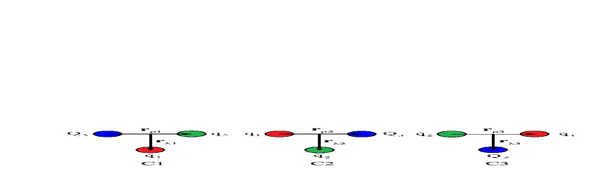
Figure 1: Jacobi coordinates for the three body system.
𝒓 λ = 𝒓 k − m i 𝒓 i + m j 𝒓 j m i + m j subscript 𝒓 𝜆 subscript 𝒓 𝑘 subscript 𝑚 𝑖 subscript 𝒓 𝑖 subscript 𝑚 𝑗 subscript 𝒓 𝑗 subscript 𝑚 𝑖 subscript 𝑚 𝑗 \displaystyle\boldsymbol{r}_{\lambda}=\boldsymbol{r}_{k}-\frac{m_{i}\boldsymbol{r}_{i}+m_{j}\boldsymbol{r}_{j}}{m_{i}+m_{j}} (1)
𝒓 ρ = 𝒓 i − 𝒓 j subscript 𝒓 𝜌 subscript 𝒓 𝑖 subscript 𝒓 𝑗 \displaystyle\boldsymbol{r}_{\rho}=\boldsymbol{r}_{i}-\boldsymbol{r}_{j} (2)
Table 1: The quark assignments (i 𝑖 i j 𝑗 j k 𝑘 k
where assignments of (i 𝑖 i j 𝑗 j k 𝑘 k c = 3 𝑐 3 c=3 c = 1 𝑐 1 c=1 c = 2 𝑐 2 c=2
𝒓 ρ 3 = α 31 ( 32 ) r 𝒓 ρ 1 ( 2 ) + β 31 ( 32 ) r 𝒓 λ 1 ( 2 ) subscript 𝒓 subscript 𝜌 3 superscript subscript 𝛼 31 32 𝑟 subscript 𝒓 subscript 𝜌 1 2 superscript subscript 𝛽 31 32 𝑟 subscript 𝒓 subscript 𝜆 1 2 \displaystyle\boldsymbol{r}_{\rho_{3}}=\alpha_{31(32)}^{r}\boldsymbol{r}_{\rho_{1(2)}}+\beta_{31(32)}^{r}\boldsymbol{r}_{\lambda_{1(2)}} (3)
𝒓 λ 3 = γ 31 ( 32 ) r 𝒓 ρ 1 ( 2 ) + δ 31 ( 32 ) r 𝒓 λ 1 ( 2 ) subscript 𝒓 subscript 𝜆 3 superscript subscript 𝛾 31 32 𝑟 subscript 𝒓 subscript 𝜌 1 2 superscript subscript 𝛿 31 32 𝑟 subscript 𝒓 𝜆 1 2 \displaystyle\boldsymbol{r}_{\lambda_{3}}=\gamma_{31(32)}^{r}\boldsymbol{r}_{\rho_{1(2)}}+\delta_{31(32)}^{r}\boldsymbol{r}_{\lambda 1(2)} (4)
where the transforming coefficients for c : 3 → 1 : 𝑐 → 3 1 c:3\rightarrow 1 3 → 2 → 3 2 3\rightarrow 2
α 31 r = − m 3 m 2 + m 3 superscript subscript 𝛼 31 𝑟 subscript 𝑚 3 subscript 𝑚 2 subscript 𝑚 3 \alpha_{31}^{r}=-\frac{m_{3}}{m_{2}+m_{3}} β 31 r = 1 superscript subscript 𝛽 31 𝑟 1 \beta_{31}^{r}=1 γ 31 r = − m 2 ( m 1 + m 2 + m 3 ) ( m 1 + m 2 ) ( m 2 + m 3 ) superscript subscript 𝛾 31 𝑟 subscript 𝑚 2 subscript 𝑚 1 subscript 𝑚 2 subscript 𝑚 3 subscript 𝑚 1 subscript 𝑚 2 subscript 𝑚 2 subscript 𝑚 3 \gamma_{31}^{r}=-\frac{m_{2}(m_{1}+m_{2}+m_{3})}{(m_{1}+m_{2})(m_{2}+m_{3})} δ 31 r = − m 1 m 1 + m 2 superscript subscript 𝛿 31 𝑟 subscript 𝑚 1 subscript 𝑚 1 subscript 𝑚 2 \delta_{31}^{r}=-\frac{m_{1}}{m_{1}+m_{2}}
α 32 r = − m 3 m 1 + m 3 superscript subscript 𝛼 32 𝑟 subscript 𝑚 3 subscript 𝑚 1 subscript 𝑚 3 \alpha_{32}^{r}=-\frac{m_{3}}{m_{1}+m_{3}} β 32 r = − 1 superscript subscript 𝛽 32 𝑟 1 \beta_{32}^{r}=-1 γ 32 r = m 1 ( m 1 + m 2 + m 3 ) ( m 1 + m 2 ) ( m 1 + m 3 ) superscript subscript 𝛾 32 𝑟 subscript 𝑚 1 subscript 𝑚 1 subscript 𝑚 2 subscript 𝑚 3 subscript 𝑚 1 subscript 𝑚 2 subscript 𝑚 1 subscript 𝑚 3 \gamma_{32}^{r}=\frac{m_{1}(m_{1}+m_{2}+m_{3})}{(m_{1}+m_{2})(m_{1}+m_{3})} δ 32 r = − m 2 m 1 + m 2 superscript subscript 𝛿 32 𝑟 subscript 𝑚 2 subscript 𝑚 1 subscript 𝑚 2 \delta_{32}^{r}=-\frac{m_{2}}{m_{1}+m_{2}}
In the following, we give a brief introduction to the Hamiltonian of relativized quark model. The relativistic Hamiltonian for a three-body system can be written asGI ; quam1
H ^ = ∑ i = 1 3 ( p i 2 + m i 2 ) 1 / 2 + ∑ i < j H ~ i j conf + ∑ i < j H ~ i j hyp + ∑ i < j H ~ i j so ^ 𝐻 superscript subscript 𝑖 1 3 superscript superscript subscript 𝑝 𝑖 2 superscript subscript 𝑚 𝑖 2 1 2 subscript 𝑖 𝑗 superscript subscript ~ 𝐻 𝑖 𝑗 conf subscript 𝑖 𝑗 superscript subscript ~ 𝐻 𝑖 𝑗 hyp subscript 𝑖 𝑗 superscript subscript ~ 𝐻 𝑖 𝑗 so \displaystyle\widehat{H}=\sum_{i=1}^{3}(p_{i}^{2}+m_{i}^{2})^{1/2}+\sum_{i<j}\widetilde{H}_{ij}^{\mathrm{conf}}+\sum_{i<j}\widetilde{H}_{ij}^{\mathrm{hyp}}+\sum_{i<j}\widetilde{H}_{ij}^{\mathrm{so}} (5)
where the first term is the relativistic kinetic energy term, H ~ conf superscript ~ 𝐻 conf \widetilde{H}^{\mathrm{conf}} S ~ ( r i j ) ~ 𝑆 subscript 𝑟 𝑖 𝑗 \widetilde{S}(r_{ij}) G ′ ( r i j ) superscript 𝐺 ′ subscript 𝑟 𝑖 𝑗 G^{\prime}(r_{ij})
H ~ i j conf = S ~ ( r i j ) + G ′ ( r i j ) subscript superscript ~ 𝐻 conf 𝑖 𝑗 ~ 𝑆 subscript 𝑟 𝑖 𝑗 superscript 𝐺 ′ subscript 𝑟 𝑖 𝑗 \displaystyle\widetilde{H}^{\mathrm{conf}}_{ij}=\widetilde{S}(r_{ij})+G^{\prime}(r_{ij}) (6)
with
S ~ ( r i j ) = − 3 4 F i ⋅ F j [ b r i j [ e − σ i j 2 r i j 2 π σ i j r i j + ( 1 + 1 2 σ i j 2 r i j 2 ) 2 π ∫ 0 σ i j r i j e − x 2 𝑑 x ] + c ] ~ 𝑆 subscript 𝑟 𝑖 𝑗 ⋅ 3 4 subscript F 𝑖 subscript F 𝑗 delimited-[] 𝑏 subscript 𝑟 𝑖 𝑗 delimited-[] superscript 𝑒 superscript subscript 𝜎 𝑖 𝑗 2 superscript subscript 𝑟 𝑖 𝑗 2 𝜋 subscript 𝜎 𝑖 𝑗 subscript 𝑟 𝑖 𝑗 1 1 2 superscript subscript 𝜎 𝑖 𝑗 2 superscript subscript 𝑟 𝑖 𝑗 2 2 𝜋 subscript superscript subscript 𝜎 𝑖 𝑗 subscript 𝑟 𝑖 𝑗 0 superscript 𝑒 superscript 𝑥 2 differential-d 𝑥 𝑐 \displaystyle\widetilde{S}(r_{ij})=-\frac{3}{4}\textbf{\emph{F}}_{i}\cdot\textbf{\emph{F}}_{j}\Big{[}br_{ij}\big{[}\frac{e^{-\sigma_{ij}^{2}r_{ij}^{2}}}{\sqrt{\pi}\sigma_{ij}r_{ij}}+\big{(}1+\frac{1}{2\sigma_{ij}^{2}r_{ij}^{2}}\big{)}\frac{2}{\sqrt{\pi}}\int^{\sigma_{ij}r_{ij}}_{0}e^{-x^{2}}dx\big{]}+c\Big{]} (7)
σ i j = s 2 [ 2 m i m j m i + m j ] 2 + σ 0 2 [ 1 2 ( 4 m i m j ( m i + m j ) 2 ) 4 + 1 2 ] subscript 𝜎 𝑖 𝑗 superscript 𝑠 2 superscript delimited-[] 2 subscript 𝑚 𝑖 subscript 𝑚 𝑗 subscript 𝑚 𝑖 subscript 𝑚 𝑗 2 superscript subscript 𝜎 0 2 delimited-[] 1 2 superscript 4 subscript 𝑚 𝑖 subscript 𝑚 𝑗 superscript subscript 𝑚 𝑖 subscript 𝑚 𝑗 2 4 1 2 \displaystyle\sigma_{ij}=\sqrt{s^{2}\Big{[}\frac{2m_{i}m_{j}}{m_{i}+m_{j}}\Big{]}^{2}+\sigma_{0}^{2}\Big{[}\frac{1}{2}\big{(}\frac{4m_{i}m_{j}}{(m_{i}+m_{j})^{2}}\big{)}^{4}+\frac{1}{2}\Big{]}} (8)
The F i ⋅ F j ⋅ subscript F 𝑖 subscript F 𝑗 \textbf{\emph{F}}_{i}\cdot\textbf{\emph{F}}_{j} F n subscript 𝐹 𝑛 F_{n}
F n = { λ n 2 for quarks , − λ n ∗ 2 for antiquarks subscript 𝐹 𝑛 cases subscript 𝜆 𝑛 2 for quarks
superscript subscript 𝜆 𝑛 2 for antiquarks
F_{n}=\left\{\begin{array}[]{l}\frac{\lambda_{n}}{2}\quad\mathrm{for}\,\mathrm{quarks},\\
-\frac{\lambda_{n}^{*}}{2}\quad\mathrm{for}\,\mathrm{antiquarks}\\
\end{array}\right. (9)
with n = 1 , 2 ⋯ 8 𝑛 1 2 ⋯ 8
n=1,2\cdots 8 G ′ ( r i j ) superscript 𝐺 ′ subscript 𝑟 𝑖 𝑗 G^{\prime}(r_{ij})
G ′ ( r i j ) = ( 1 + p i j 2 E i E j ) 1 2 G ~ ( r i j ) ( 1 + p i j 2 E i E j ) 1 2 superscript 𝐺 ′ subscript 𝑟 𝑖 𝑗 superscript 1 subscript superscript 𝑝 2 𝑖 𝑗 subscript 𝐸 𝑖 subscript 𝐸 𝑗 1 2 ~ 𝐺 subscript 𝑟 𝑖 𝑗 superscript 1 subscript superscript 𝑝 2 𝑖 𝑗 subscript 𝐸 𝑖 subscript 𝐸 𝑗 1 2 \displaystyle G^{\prime}(r_{ij})=\Big{(}1+\frac{p^{2}_{ij}}{E_{i}E_{j}}\Big{)}^{\frac{1}{2}}\widetilde{G}(r_{ij})\Big{(}1+\frac{p^{2}_{ij}}{E_{i}E_{j}}\Big{)}^{\frac{1}{2}} (10)
with
G ~ ( r i j ) = F i ⋅ F j ∑ k = 1 3 2 α k 3 π r i j ∫ 0 τ k r i j e − x 2 𝑑 x ~ 𝐺 subscript 𝑟 𝑖 𝑗 ⋅ subscript F 𝑖 subscript F 𝑗 superscript subscript 𝑘 1 3 2 subscript 𝛼 𝑘 3 𝜋 subscript 𝑟 𝑖 𝑗 subscript superscript subscript 𝜏 𝑘 subscript 𝑟 𝑖 𝑗 0 superscript 𝑒 superscript 𝑥 2 differential-d 𝑥 \displaystyle\widetilde{G}(r_{ij})=\textbf{\emph{F}}_{i}\cdot\textbf{\emph{F}}_{j}\mathop{\sum}\limits_{k=1}^{3}\frac{2\alpha_{k}}{3\sqrt{\pi}r_{ij}}\int^{\tau_{k}r_{ij}}_{0}e^{-x^{2}}dx (11)
and τ k = 1 1 σ i j 2 + 1 γ k 2 subscript 𝜏 𝑘 1 1 superscript subscript 𝜎 𝑖 𝑗 2 1 superscript subscript 𝛾 𝑘 2 \tau_{k}=\frac{1}{\sqrt{\frac{1}{\sigma_{ij}^{2}}+\frac{1}{\gamma_{k}^{2}}}}
In, Eq.(5), H ~ hyp superscript ~ 𝐻 hyp \widetilde{H}^{\mathrm{hyp}}
H ~ i j hyp = H ~ i j tensor + H ~ i j c subscript superscript ~ 𝐻 hyp 𝑖 𝑗 subscript superscript ~ 𝐻 tensor 𝑖 𝑗 superscript subscript ~ 𝐻 𝑖 𝑗 c \displaystyle\widetilde{H}^{\mathrm{hyp}}_{ij}=\widetilde{H}^{\mathrm{tensor}}_{ij}+\widetilde{H}_{ij}^{\mathrm{c}} (12)
with
H ~ i j tensor = − ( S i ⋅ r i j S j ⋅ r i j / r i j 2 − 1 3 S i ⋅ S j m i m j ) × ( ∂ 2 ∂ r i j 2 − 1 r i j ∂ ∂ r i j ) G ~ i j t , subscript superscript ~ 𝐻 tensor 𝑖 𝑗 ⋅ ⋅ subscript S 𝑖 subscript r 𝑖 𝑗 subscript S 𝑗 subscript r 𝑖 𝑗 superscript subscript 𝑟 𝑖 𝑗 2 ⋅ 1 3 subscript S 𝑖 subscript S 𝑗 subscript 𝑚 𝑖 subscript 𝑚 𝑗 superscript 2 superscript subscript 𝑟 𝑖 𝑗 2 1 subscript 𝑟 𝑖 𝑗 subscript 𝑟 𝑖 𝑗 superscript subscript ~ 𝐺 𝑖 𝑗 t \displaystyle\widetilde{H}^{\mathrm{tensor}}_{ij}=-\Big{(}\frac{\textbf{S}_{i}\cdot\textbf{r}_{ij}\textbf{S}_{j}\cdot\textbf{r}_{ij}/r_{ij}^{2}-\frac{1}{3}\textbf{S}_{i}\cdot\textbf{S}_{j}}{m_{i}m_{j}}\Big{)}\times\Big{(}\frac{\partial^{2}}{\partial r_{ij}^{2}}-\frac{1}{r_{ij}}\frac{\partial}{\partial r_{ij}}\Big{)}\widetilde{G}_{ij}^{\mathrm{t}}, (13)
H ~ i j c = 2 S i ⋅ S j 3 m i m j ▽ 2 G ~ i j c subscript superscript ~ 𝐻 c 𝑖 𝑗 superscript ▽ 2 ⋅ 2 subscript S 𝑖 subscript S 𝑗 3 subscript 𝑚 𝑖 subscript 𝑚 𝑗 superscript subscript ~ 𝐺 𝑖 𝑗 c \displaystyle\widetilde{H}^{\mathrm{c}}_{ij}=\frac{2\textbf{S}_{i}\cdot\textbf{S}_{j}}{3m_{i}m_{j}}\bigtriangledown^{2}\widetilde{G}_{ij}^{\mathrm{c}} (14)
For the spin-orbit interaction, it can be divided into two parts which can be written as,
H ~ i j so = H ~ i j so ( v ) + H ~ i j so ( s ) , subscript superscript ~ 𝐻 so 𝑖 𝑗 subscript superscript ~ 𝐻 so v 𝑖 𝑗 superscript subscript ~ 𝐻 𝑖 𝑗 so s \displaystyle\widetilde{H}^{\mathrm{so}}_{ij}=\widetilde{H}^{\mathrm{so(v)}}_{ij}+\widetilde{H}_{ij}^{\mathrm{so(s)}}, (15)
with
H ~ i j so ( v ) = S i ⋅ L i j 2 m i 2 r i j ∂ G ~ i i so ( v ) ∂ r i j + S j ⋅ L i j 2 m j 2 r i j ∂ G ~ j j so ( v ) ∂ r i j + ( S i + S j ) ⋅ L i j m i m j r i j 1 r i j ∂ G ~ i j so ( v ) ∂ r i j subscript superscript ~ 𝐻 so v 𝑖 𝑗 ⋅ subscript S 𝑖 subscript L 𝑖 𝑗 2 superscript subscript 𝑚 𝑖 2 subscript 𝑟 𝑖 𝑗 subscript superscript ~ 𝐺 so v 𝑖 𝑖 subscript 𝑟 𝑖 𝑗 ⋅ subscript S 𝑗 subscript L 𝑖 𝑗 2 superscript subscript 𝑚 𝑗 2 subscript 𝑟 𝑖 𝑗 subscript superscript ~ 𝐺 so v 𝑗 𝑗 subscript 𝑟 𝑖 𝑗 ⋅ subscript S 𝑖 subscript S 𝑗 subscript L 𝑖 𝑗 subscript 𝑚 𝑖 subscript 𝑚 𝑗 subscript 𝑟 𝑖 𝑗 1 subscript 𝑟 𝑖 𝑗 subscript superscript ~ 𝐺 so v 𝑖 𝑗 subscript 𝑟 𝑖 𝑗 \displaystyle\widetilde{H}^{\mathrm{so(v)}}_{ij}=\frac{\textbf{S}_{i}\cdot\textbf{L}_{ij}}{2m_{i}^{2}r_{ij}}\frac{\partial\widetilde{G}^{\mathrm{so(v)}}_{ii}}{\partial r_{ij}}+\frac{\textbf{S}_{j}\cdot\textbf{L}_{ij}}{2m_{j}^{2}r_{ij}}\frac{\partial\widetilde{G}^{\mathrm{so(v)}}_{jj}}{\partial r_{ij}}+\frac{(\textbf{S}_{i}+\textbf{S}_{j})\cdot\textbf{L}_{ij}}{m_{i}m_{j}r_{ij}}\frac{1}{r_{ij}}\frac{\partial\widetilde{G}^{\mathrm{so(v)}}_{ij}}{\partial r_{ij}} (16)
and
H ~ i j so ( s ) = − S i ⋅ L i j 2 m i 2 r i j ∂ S ~ i i so ( s ) ∂ r i j − S j ⋅ L i j 2 m j 2 r i j ∂ S ~ j j so ( s ) ∂ r i j subscript superscript ~ 𝐻 so s 𝑖 𝑗 ⋅ subscript S 𝑖 subscript L 𝑖 𝑗 2 superscript subscript 𝑚 𝑖 2 subscript 𝑟 𝑖 𝑗 subscript superscript ~ 𝑆 so s 𝑖 𝑖 subscript 𝑟 𝑖 𝑗 ⋅ subscript S 𝑗 subscript L 𝑖 𝑗 2 superscript subscript 𝑚 𝑗 2 subscript 𝑟 𝑖 𝑗 subscript superscript ~ 𝑆 so s 𝑗 𝑗 subscript 𝑟 𝑖 𝑗 \displaystyle\widetilde{H}^{\mathrm{so(s)}}_{ij}=-\frac{\textbf{S}_{i}\cdot\textbf{L}_{ij}}{2m_{i}^{2}r_{ij}}\frac{\partial\widetilde{S}^{\mathrm{so(s)}}_{ii}}{\partial r_{ij}}-\frac{\textbf{S}_{j}\cdot\textbf{L}_{ij}}{2m_{j}^{2}r_{ij}}\frac{\partial\widetilde{S}^{\mathrm{so(s)}}_{jj}}{\partial r_{ij}} (17)
In Eqs.(13),(14),(16) and (17), G ~ i j t subscript superscript ~ 𝐺 t 𝑖 𝑗 \widetilde{G}^{\mathrm{t}}_{ij} G ~ i j c subscript superscript ~ 𝐺 c 𝑖 𝑗 \widetilde{G}^{\mathrm{c}}_{ij} G ~ i j so ( v ) subscript superscript ~ 𝐺 so v 𝑖 𝑗 \widetilde{G}^{\mathrm{so(v)}}_{ij} S ~ i i so ( s ) subscript superscript ~ 𝑆 so s 𝑖 𝑖 \widetilde{S}^{\mathrm{so(s)}}_{ii} G ~ ( r i j ) ~ 𝐺 subscript 𝑟 𝑖 𝑗 \widetilde{G}(r_{ij}) S ~ ( r i j ) ~ 𝑆 subscript 𝑟 𝑖 𝑗 \widetilde{S}(r_{ij})
G i j t = ( m i m j E i E j ) 1 2 + ϵ t G ~ ( r i j ) ( m i m j E i E j ) 1 2 + ϵ t subscript superscript 𝐺 t 𝑖 𝑗 superscript subscript 𝑚 𝑖 subscript 𝑚 𝑗 subscript 𝐸 𝑖 subscript 𝐸 𝑗 1 2 subscript italic-ϵ t ~ 𝐺 subscript 𝑟 𝑖 𝑗 superscript subscript 𝑚 𝑖 subscript 𝑚 𝑗 subscript 𝐸 𝑖 subscript 𝐸 𝑗 1 2 subscript italic-ϵ t \displaystyle G^{\mathrm{t}}_{ij}=\Big{(}\frac{m_{i}m_{j}}{E_{i}E_{j}}\Big{)}^{\frac{1}{2}+\epsilon_{\mathrm{t}}}\widetilde{G}(r_{ij})\Big{(}\frac{m_{i}m_{j}}{E_{i}E_{j}}\Big{)}^{\frac{1}{2}+\epsilon_{\mathrm{t}}} (18)
G i j c = ( m i m j E i E j ) 1 2 + ϵ c G ~ ( r i j ) ( m i m j E i E j ) 1 2 + ϵ c subscript superscript 𝐺 c 𝑖 𝑗 superscript subscript 𝑚 𝑖 subscript 𝑚 𝑗 subscript 𝐸 𝑖 subscript 𝐸 𝑗 1 2 subscript italic-ϵ c ~ 𝐺 subscript 𝑟 𝑖 𝑗 superscript subscript 𝑚 𝑖 subscript 𝑚 𝑗 subscript 𝐸 𝑖 subscript 𝐸 𝑗 1 2 subscript italic-ϵ c \displaystyle G^{\mathrm{c}}_{ij}=\Big{(}\frac{m_{i}m_{j}}{E_{i}E_{j}}\Big{)}^{\frac{1}{2}+\epsilon_{\mathrm{c}}}\widetilde{G}(r_{ij})\Big{(}\frac{m_{i}m_{j}}{E_{i}E_{j}}\Big{)}^{\frac{1}{2}+\epsilon_{\mathrm{c}}} (19)
G i j so ( v ) = ( m i m j E i E j ) 1 2 + ϵ so ( v ) G ~ ( r i j ) ( m i m j E i E j ) 1 2 + ϵ so ( v ) subscript superscript 𝐺 so v 𝑖 𝑗 superscript subscript 𝑚 𝑖 subscript 𝑚 𝑗 subscript 𝐸 𝑖 subscript 𝐸 𝑗 1 2 subscript italic-ϵ so v ~ 𝐺 subscript 𝑟 𝑖 𝑗 superscript subscript 𝑚 𝑖 subscript 𝑚 𝑗 subscript 𝐸 𝑖 subscript 𝐸 𝑗 1 2 subscript italic-ϵ so v \displaystyle G^{\mathrm{so(v)}}_{ij}=\Big{(}\frac{m_{i}m_{j}}{E_{i}E_{j}}\Big{)}^{\frac{1}{2}+\epsilon_{\mathrm{so(v)}}}\widetilde{G}(r_{ij})\Big{(}\frac{m_{i}m_{j}}{E_{i}E_{j}}\Big{)}^{\frac{1}{2}+\epsilon_{\mathrm{so(v)}}} (20)
S ~ i i so ( s ) = ( m i 2 E i 2 ) 1 2 + ϵ so ( s ) S ~ ( r i j ) ( m i 2 E i 2 ) 1 2 + ϵ so ( s ) subscript superscript ~ 𝑆 so s 𝑖 𝑖 superscript superscript subscript 𝑚 𝑖 2 superscript subscript 𝐸 𝑖 2 1 2 subscript italic-ϵ so s ~ 𝑆 subscript 𝑟 𝑖 𝑗 superscript superscript subscript 𝑚 𝑖 2 superscript subscript 𝐸 𝑖 2 1 2 subscript italic-ϵ so s \displaystyle\widetilde{S}^{\mathrm{so(s)}}_{ii}=\Big{(}\frac{m_{i}^{2}}{E_{i}^{2}}\Big{)}^{\frac{1}{2}+\epsilon_{\mathrm{so(s)}}}\widetilde{S}(r_{ij})\Big{(}\frac{m_{i}^{2}}{E_{i}^{2}}\Big{)}^{\frac{1}{2}+\epsilon_{\mathrm{so(s)}}} (21)
with E i = m i 2 + p i j 2 subscript 𝐸 𝑖 superscript subscript 𝑚 𝑖 2 superscript subscript 𝑝 𝑖 𝑗 2 E_{i}=\sqrt{m_{i}^{2}+p_{ij}^{2}} ϵ t subscript italic-ϵ t \epsilon_{\mathrm{t}} ϵ c subscript italic-ϵ c \epsilon_{\mathrm{c}} ϵ so ( v ) subscript italic-ϵ so v \epsilon_{\mathrm{so(v)}} ϵ so ( s ) subscript italic-ϵ so s \epsilon_{\mathrm{so(s)}} p i j subscript 𝑝 𝑖 𝑗 p_{ij} i j 𝑖 𝑗 ij p 23 subscript 𝑝 23 p_{23} p 13 subscript 𝑝 13 p_{13} p 12 subscript 𝑝 12 p_{12} p ρ 1 subscript 𝑝 subscript 𝜌 1 p_{\rho_{1}} p ρ 2 subscript 𝑝 subscript 𝜌 2 p_{\rho_{2}} p ρ 3 subscript 𝑝 subscript 𝜌 3 p_{\rho_{3}}
2.2 Wave function of single heavy baryon
In quark model scheme, the full wave function for a definite baryon is built from a linear superposition of the channel wave function, which can be written as,
Ψ f u l l J M = ∑ c α C c , α Ψ J M c ( 𝒓 ρ c , 𝒓 λ c ) superscript subscript Ψ 𝑓 𝑢 𝑙 𝑙 𝐽 𝑀 subscript 𝑐 𝛼 subscript 𝐶 𝑐 𝛼
superscript subscript Ψ 𝐽 𝑀 𝑐 subscript 𝒓 subscript 𝜌 𝑐 subscript 𝒓 subscript 𝜆 𝑐 \displaystyle\Psi_{full}^{JM}=\sum_{c\alpha}C_{c,\alpha}\Psi_{JM}^{c}(\boldsymbol{r}_{\rho_{c}},\boldsymbol{r}_{\lambda_{c}}) (22)
where the index α 𝛼 \alpha n ρ subscript 𝑛 𝜌 n_{\rho} n λ subscript 𝑛 𝜆 n_{\lambda} l ρ subscript 𝑙 𝜌 l_{\rho} l λ subscript 𝑙 𝜆 l_{\lambda} L 𝐿 L s 𝑠 s j 𝑗 j c 𝑐 c c = 1 , 2 , 3 𝑐 1 2 3
c=1,2,3 Ψ J M c ( 𝒓 ρ c , 𝒓 λ c ) superscript subscript Ψ 𝐽 𝑀 𝑐 subscript 𝒓 subscript 𝜌 𝑐 subscript 𝒓 subscript 𝜆 𝑐 \Psi_{JM}^{c}(\boldsymbol{r}_{\rho_{c}},\boldsymbol{r}_{\lambda_{c}}) c 𝑐 c ϕ color subscript italic-ϕ color \phi_{\mathrm{color}} ϕ flavor subscript italic-ϕ flavor \phi_{\mathrm{flavor}} ψ J M c superscript subscript 𝜓 𝐽 𝑀 𝑐 \psi_{JM}^{c}
Ψ J M c ( 𝒓 ρ c , 𝒓 λ c ) = ϕ color ⊗ ϕ flavor ⊗ ψ J M c superscript subscript Ψ 𝐽 𝑀 𝑐 subscript 𝒓 subscript 𝜌 𝑐 subscript 𝒓 subscript 𝜆 𝑐 tensor-product subscript italic-ϕ color subscript italic-ϕ flavor superscript subscript 𝜓 𝐽 𝑀 𝑐 \displaystyle\Psi_{JM}^{c}(\boldsymbol{r}_{\rho_{c}},\boldsymbol{r}_{\lambda_{c}})=\phi_{\mathrm{color}}\otimes\phi_{\mathrm{flavor}}\otimes\psi_{JM}^{c} (23)
with
ϕ color = 1 6 ( r g b − r b g + g b r − g r b + b r g − b g r ) , subscript italic-ϕ color 1 6 𝑟 𝑔 𝑏 𝑟 𝑏 𝑔 𝑔 𝑏 𝑟 𝑔 𝑟 𝑏 𝑏 𝑟 𝑔 𝑏 𝑔 𝑟 \displaystyle\phi_{\mathrm{color}}=\frac{1}{\sqrt{6}}\big{(}rgb-rbg+gbr-grb+brg-bgr\big{)}, (24)
ψ J M c = [ [ [ χ 1 / 2 ( q ) χ 1 / 2 ( q ) ] s , m s Φ l ρ , l λ , L c ] j , m j χ 1 / 2 ( Q ) ] J M , superscript subscript 𝜓 𝐽 𝑀 𝑐 subscript delimited-[] subscript delimited-[] subscript delimited-[] subscript 𝜒 1 2 𝑞 subscript 𝜒 1 2 𝑞 𝑠 subscript 𝑚 𝑠
subscript superscript Φ 𝑐 subscript 𝑙 𝜌 subscript 𝑙 𝜆 𝐿
𝑗 subscript 𝑚 𝑗
subscript 𝜒 1 2 𝑄 𝐽 𝑀 \displaystyle\psi_{JM}^{c}=\Big{[}\big{[}[\chi_{1/2}(q)\chi_{1/2}(q)]_{s,m_{s}}\Phi^{c}_{l_{\rho},l_{\lambda},L}\big{]}_{j,m_{j}}\chi_{1/2}(Q)\Big{]}_{JM}, (25)
where r 𝑟 r g 𝑔 g b 𝑏 b χ 1 / 2 subscript 𝜒 1 2 \chi_{1/2} 6 F subscript 6 𝐹 6_{F} 3 ¯ F subscript ¯ 3 𝐹 \overline{3}_{F} Σ Q subscript Σ 𝑄 \Sigma_{Q} Ω Q subscript Ω 𝑄 \Omega_{Q} ϕ 6 F subscript italic-ϕ subscript 6 𝐹 \phi_{6_{F}} Λ Q subscript Λ 𝑄 \Lambda_{Q} ϕ 3 ¯ F subscript italic-ϕ subscript ¯ 3 𝐹 \phi_{\overline{3}_{F}} Φ l ρ , l λ , L c subscript superscript Φ 𝑐 subscript 𝑙 𝜌 subscript 𝑙 𝜆 𝐿
\Phi^{c}_{l_{\rho},l_{\lambda},L} ρ 𝜌 \rho λ 𝜆 \lambda
Φ l ρ , l λ , L c = [ ϕ l ρ m l ρ ( 𝒓 ρ c ) ϕ l λ m l λ ( 𝒓 λ c ) ] L c = 1 , 2 , 3 formulae-sequence subscript superscript Φ 𝑐 subscript 𝑙 𝜌 subscript 𝑙 𝜆 𝐿
subscript delimited-[] subscript italic-ϕ subscript 𝑙 𝜌 subscript 𝑚 subscript 𝑙 𝜌 subscript 𝒓 subscript 𝜌 𝑐 subscript italic-ϕ subscript 𝑙 𝜆 subscript 𝑚 subscript 𝑙 𝜆 subscript 𝒓 subscript 𝜆 𝑐 𝐿 𝑐 1 2 3
\displaystyle\Phi^{c}_{l_{\rho},l_{\lambda},L}=\Big{[}\phi_{l_{\rho}m_{l_{\rho}}}(\boldsymbol{r}_{\rho_{c}})\phi_{l_{\lambda}m_{l_{\lambda}}}(\boldsymbol{r}_{\lambda_{c}})\Big{]}_{L}\quad c=1,2,3 (26)
In this work, the spatial wave function of a three-body system is expanded in terms of a set of Gaussian basis functions. Thus, ϕ l ρ m l ρ ( 𝒓 ρ c ) subscript italic-ϕ subscript 𝑙 𝜌 subscript 𝑚 subscript 𝑙 𝜌 subscript 𝒓 subscript 𝜌 𝑐 \phi_{l_{\rho}m_{l_{\rho}}}(\boldsymbol{r}_{\rho_{c}}) ϕ l λ m l λ ( 𝒓 λ c ) subscript italic-ϕ subscript 𝑙 𝜆 subscript 𝑚 subscript 𝑙 𝜆 subscript 𝒓 subscript 𝜆 𝑐 \phi_{l_{\lambda}m_{l_{\lambda}}}(\boldsymbol{r}_{\lambda_{c}})
ϕ n ρ l ρ m l ρ ( 𝒓 ρ c ) = N n ρ l ρ r ρ c l ρ e − ν n ρ r ρ c 2 Y l ρ m l ρ ( 𝒓 ^ ρ c ) subscript italic-ϕ subscript 𝑛 𝜌 subscript 𝑙 𝜌 subscript 𝑚 subscript 𝑙 𝜌 subscript 𝒓 subscript 𝜌 𝑐 subscript 𝑁 subscript 𝑛 𝜌 subscript 𝑙 𝜌 superscript subscript 𝑟 subscript 𝜌 𝑐 subscript 𝑙 𝜌 superscript 𝑒 subscript 𝜈 subscript 𝑛 𝜌 superscript subscript 𝑟 subscript 𝜌 𝑐 2 subscript 𝑌 subscript 𝑙 𝜌 subscript 𝑚 subscript 𝑙 𝜌 subscript ^ 𝒓 subscript 𝜌 𝑐 \displaystyle\phi_{n_{\rho}l_{\rho}m_{l_{\rho}}}(\boldsymbol{r}_{\rho_{c}})=N_{n_{\rho}l_{\rho}}r_{\rho_{c}}^{l_{\rho}}e^{-\nu_{n_{\rho}}r_{\rho_{c}}^{2}}Y_{l_{\rho}m_{l_{\rho}}}(\hat{\boldsymbol{r}}_{\rho_{c}}) (27)
ϕ n λ l λ m l λ ( 𝒓 λ c ) = N n λ l λ r λ c l λ e − ν n λ r λ c 2 Y l λ m l λ ( 𝒓 ^ λ c ) subscript italic-ϕ subscript 𝑛 𝜆 subscript 𝑙 𝜆 subscript 𝑚 subscript 𝑙 𝜆 subscript 𝒓 subscript 𝜆 𝑐 subscript 𝑁 subscript 𝑛 𝜆 subscript 𝑙 𝜆 superscript subscript 𝑟 subscript 𝜆 𝑐 subscript 𝑙 𝜆 superscript 𝑒 subscript 𝜈 subscript 𝑛 𝜆 superscript subscript 𝑟 subscript 𝜆 𝑐 2 subscript 𝑌 subscript 𝑙 𝜆 subscript 𝑚 subscript 𝑙 𝜆 subscript ^ 𝒓 subscript 𝜆 𝑐 \displaystyle\phi_{n_{\lambda}l_{\lambda}m_{l_{\lambda}}}(\boldsymbol{r}_{\lambda_{c}})=N_{n_{\lambda}l_{\lambda}}r_{\lambda_{c}}^{l_{\lambda}}e^{-\nu_{n_{\lambda}}r_{\lambda_{c}}^{2}}Y_{l_{\lambda}m_{l_{\lambda}}}(\hat{\boldsymbol{r}}_{\lambda_{c}}) (28)
with
N n ρ l ρ = 2 l ρ + 2 ( 2 ν n ρ ) l ρ + 3 / 2 π ( 2 l ρ + 1 ) !! subscript 𝑁 subscript 𝑛 𝜌 subscript 𝑙 𝜌 superscript 2 subscript 𝑙 𝜌 2 superscript 2 subscript 𝜈 subscript 𝑛 𝜌 subscript 𝑙 𝜌 3 2 𝜋 double-factorial 2 subscript 𝑙 𝜌 1 \displaystyle N_{n_{\rho}l_{\rho}}=\sqrt{\frac{2^{l_{\rho}+2}(2\nu_{n_{\rho}})^{l_{\rho}+3/2}}{\sqrt{\pi}(2l_{\rho}+1)!!}} (29)
N n λ l λ = 2 l λ + 2 ( 2 ν n λ ) l λ + 3 / 2 π ( 2 l λ + 1 ) !! subscript 𝑁 subscript 𝑛 𝜆 subscript 𝑙 𝜆 superscript 2 subscript 𝑙 𝜆 2 superscript 2 subscript 𝜈 subscript 𝑛 𝜆 subscript 𝑙 𝜆 3 2 𝜋 double-factorial 2 subscript 𝑙 𝜆 1 \displaystyle N_{n_{\lambda}l_{\lambda}}=\sqrt{\frac{2^{l_{\lambda}+2}(2\nu_{n_{\lambda}})^{l_{\lambda}+3/2}}{\sqrt{\pi}(2l_{\lambda}+1)!!}} (30)
ν n ρ = 1 r n ρ 2 , r n ρ = r a [ r a m a x r a ] n − 1 n m a x − 1 ( n = 1 , ⋯ , n m a x ) formulae-sequence subscript 𝜈 subscript 𝑛 𝜌 1 superscript subscript 𝑟 subscript 𝑛 𝜌 2 subscript 𝑟 subscript 𝑛 𝜌 subscript 𝑟 𝑎 superscript delimited-[] subscript 𝑟 𝑎 𝑚 𝑎 𝑥 subscript 𝑟 𝑎 𝑛 1 subscript 𝑛 𝑚 𝑎 𝑥 1 𝑛 1 ⋯ subscript 𝑛 𝑚 𝑎 𝑥
\displaystyle\nu_{n_{\rho}}=\frac{1}{r_{n_{\rho}}^{2}},\quad r_{n_{\rho}}=r_{a}\Big{[}\frac{r_{amax}}{r_{a}}\Big{]}^{\frac{n-1}{n_{max}-1}}\quad(n=1,\cdots,n_{max}) (31)
ν n λ = 1 r n λ 2 , r n λ = r b [ r b m a x r b ] n − 1 n m a x − 1 ( n = 1 , ⋯ , n m a x ) formulae-sequence subscript 𝜈 subscript 𝑛 𝜆 1 superscript subscript 𝑟 subscript 𝑛 𝜆 2 subscript 𝑟 subscript 𝑛 𝜆 subscript 𝑟 𝑏 superscript delimited-[] subscript 𝑟 𝑏 𝑚 𝑎 𝑥 subscript 𝑟 𝑏 𝑛 1 subscript 𝑛 𝑚 𝑎 𝑥 1 𝑛 1 ⋯ subscript 𝑛 𝑚 𝑎 𝑥
\displaystyle\nu_{n_{\lambda}}=\frac{1}{r_{n_{\lambda}}^{2}},\quad r_{n_{\lambda}}=r_{b}\Big{[}\frac{r_{bmax}}{r_{b}}\Big{]}^{\frac{n-1}{n_{max}-1}}\quad(n=1,\cdots,n_{max}) (32)
where r a subscript 𝑟 𝑎 r_{a} r b subscript 𝑟 𝑏 r_{b} r a m a x subscript 𝑟 𝑎 𝑚 𝑎 𝑥 r_{amax} r b m a x subscript 𝑟 𝑏 𝑚 𝑎 𝑥 r_{bmax} r a = r b subscript 𝑟 𝑎 subscript 𝑟 𝑏 r_{a}=r_{b} r a m a x = r b m a x subscript 𝑟 𝑎 𝑚 𝑎 𝑥 subscript 𝑟 𝑏 𝑚 𝑎 𝑥 r_{amax}=r_{bmax} n m a x subscript 𝑛 𝑚 𝑎 𝑥 n_{max}
ϕ n ρ l ρ m l ρ ( 𝒑 ρ c ) = N n ρ l ρ ′ p ρ c l ρ e − p ρ c 2 4 ν n ρ Y l ρ m l ρ ( 𝒑 ^ ρ c ) subscript italic-ϕ subscript 𝑛 𝜌 subscript 𝑙 𝜌 subscript 𝑚 subscript 𝑙 𝜌 subscript 𝒑 subscript 𝜌 𝑐 subscript superscript 𝑁 ′ subscript 𝑛 𝜌 subscript 𝑙 𝜌 superscript subscript 𝑝 subscript 𝜌 𝑐 subscript 𝑙 𝜌 superscript 𝑒 superscript subscript 𝑝 subscript 𝜌 𝑐 2 4 subscript 𝜈 subscript 𝑛 𝜌 subscript 𝑌 subscript 𝑙 𝜌 subscript 𝑚 subscript 𝑙 𝜌 subscript ^ 𝒑 subscript 𝜌 𝑐 \displaystyle\phi_{n_{\rho}l_{\rho}m_{l_{\rho}}}(\boldsymbol{p}_{\rho_{c}})=N^{\prime}_{n_{\rho}l_{\rho}}p_{\rho_{c}}^{l_{\rho}}e^{-\frac{p_{\rho_{c}}^{2}}{4\nu_{n_{\rho}}}}Y_{l_{\rho}m_{l_{\rho}}}(\hat{\boldsymbol{p}}_{\rho_{c}}) (33)
ϕ n λ l λ m l λ ( 𝒑 λ c ) = N n λ l λ ′ p λ c l λ e − p λ c 2 4 ν n λ Y l λ m l λ ( 𝒑 ^ λ c ) subscript italic-ϕ subscript 𝑛 𝜆 subscript 𝑙 𝜆 subscript 𝑚 subscript 𝑙 𝜆 subscript 𝒑 subscript 𝜆 𝑐 subscript superscript 𝑁 ′ subscript 𝑛 𝜆 subscript 𝑙 𝜆 superscript subscript 𝑝 subscript 𝜆 𝑐 subscript 𝑙 𝜆 superscript 𝑒 superscript subscript 𝑝 subscript 𝜆 𝑐 2 4 subscript 𝜈 subscript 𝑛 𝜆 subscript 𝑌 subscript 𝑙 𝜆 subscript 𝑚 subscript 𝑙 𝜆 subscript ^ 𝒑 subscript 𝜆 𝑐 \displaystyle\phi_{n_{\lambda}l_{\lambda}m_{l_{\lambda}}}(\boldsymbol{p}_{\lambda_{c}})=N^{\prime}_{n_{\lambda}l_{\lambda}}p_{\lambda_{c}}^{l_{\lambda}}e^{-\frac{p_{\lambda_{c}}^{2}}{4\nu_{n_{\lambda}}}}Y_{l_{\lambda}m_{l_{\lambda}}}(\hat{\boldsymbol{p}}_{\lambda_{c}}) (34)
with
N n ρ l ρ ′ = ( − i ) l ρ 2 l ρ + 2 π ( 2 ν n ρ ) l ρ + 3 / 2 ( 2 l ρ + 1 ) !! subscript superscript 𝑁 ′ subscript 𝑛 𝜌 subscript 𝑙 𝜌 superscript 𝑖 subscript 𝑙 𝜌 superscript 2 subscript 𝑙 𝜌 2 𝜋 superscript 2 subscript 𝜈 subscript 𝑛 𝜌 subscript 𝑙 𝜌 3 2 double-factorial 2 subscript 𝑙 𝜌 1 \displaystyle N^{\prime}_{n_{\rho}l_{\rho}}=(-i)^{l_{\rho}}\sqrt{\frac{2^{l_{\rho}+2}}{\sqrt{\pi}(2\nu_{n_{\rho}})^{l_{\rho}+3/2}(2l_{\rho}+1)!!}} (35)
N n λ l λ ′ = ( − i ) l λ 2 l λ + 2 π ( 2 ν n λ ) l λ + 3 / 2 ( 2 l λ + 1 ) !! subscript superscript 𝑁 ′ subscript 𝑛 𝜆 subscript 𝑙 𝜆 superscript 𝑖 subscript 𝑙 𝜆 superscript 2 subscript 𝑙 𝜆 2 𝜋 superscript 2 subscript 𝜈 subscript 𝑛 𝜆 subscript 𝑙 𝜆 3 2 double-factorial 2 subscript 𝑙 𝜆 1 \displaystyle N^{\prime}_{n_{\lambda}l_{\lambda}}=(-i)^{l_{\lambda}}\sqrt{\frac{2^{l_{\lambda}+2}}{\sqrt{\pi}(2\nu_{n_{\lambda}})^{l_{\lambda}+3/2}(2l_{\lambda}+1)!!}} (36)
In the heavy quark limit, one heavy quark within the heavy baryon system is decoupled from two light quarks. Under this picture, the interactions
which depend on the spin of the heavy quark disappear. Thus, two states whose quantum number are J = j + 1 / 2 𝐽 𝑗 1 2 J=j+1/2 J = j − 1 / 2 𝐽 𝑗 1 2 J=j-1/2 j 𝑗 j 3 3 3 ρ 𝜌 \rho λ 𝜆 \lambda λ 𝜆 \lambda ρ 𝜌 \rho quam4 λ 𝜆 \lambda ρ 𝜌 \rho P 𝑃 P P 𝑃 P λ 𝜆 \lambda λ 𝜆 \lambda ρ 𝜌 \rho λ 𝜆 \lambda ρ 𝜌 \rho 3 3 3
Ψ f u l l J M = ∑ n ρ , n λ C n ρ , n λ Ψ J M 3 ( 𝒓 ρ 3 , 𝒓 λ 3 ) superscript subscript Ψ 𝑓 𝑢 𝑙 𝑙 𝐽 𝑀 subscript subscript 𝑛 𝜌 subscript 𝑛 𝜆
subscript 𝐶 subscript 𝑛 𝜌 subscript 𝑛 𝜆
superscript subscript Ψ 𝐽 𝑀 3 subscript 𝒓 subscript 𝜌 3 subscript 𝒓 subscript 𝜆 3 \displaystyle\Psi_{full}^{JM}=\sum_{n_{{}_{\rho}},n_{{}_{\lambda}}}C_{n_{{}_{\rho}},n_{{}_{\lambda}}}\Psi_{JM}^{3}(\boldsymbol{r}_{\rho_{3}},\boldsymbol{r}_{\lambda_{3}}) (37)
2.3 Evaluations of the matrix elements
In the calculations of the Hamiltonian matrix elements of three-body system, particularly when
complicated interactions are employed, integrations over all of the radial and angular coordinates become
laborious even with Gaussian basis functions. This process can be simplified by introducing the ISG basis functions. For Jacobi coordinates ρ 𝜌 \rho λ 𝜆 \lambda 3 3 3 IGEM
ϕ n ρ l ρ m l ρ ( 𝒓 ρ ) = N n ρ l ρ lim ε → 0 1 ( ν n ρ ε ) l ρ ∑ k = 1 k m a x C l ρ m l ρ , k e − ν n ρ ( 𝒓 ρ − ε D l ρ m l ρ , k ) 2 subscript italic-ϕ subscript 𝑛 𝜌 subscript 𝑙 𝜌 subscript 𝑚 subscript 𝑙 𝜌 subscript 𝒓 𝜌 subscript 𝑁 subscript 𝑛 𝜌 subscript 𝑙 𝜌 subscript → 𝜀 0 1 superscript subscript 𝜈 subscript 𝑛 𝜌 𝜀 subscript 𝑙 𝜌 superscript subscript 𝑘 1 subscript 𝑘 𝑚 𝑎 𝑥 subscript 𝐶 subscript 𝑙 𝜌 subscript 𝑚 subscript 𝑙 𝜌 𝑘
superscript 𝑒 subscript 𝜈 subscript 𝑛 𝜌 superscript subscript 𝒓 𝜌 𝜀 subscript D subscript 𝑙 𝜌 subscript 𝑚 subscript 𝑙 𝜌 𝑘
2 \displaystyle\phi_{n_{\rho}l_{\rho}m_{l_{\rho}}}(\boldsymbol{r}_{\rho})=N_{n_{\rho}l_{\rho}}\lim_{\varepsilon\rightarrow 0}\frac{1}{(\nu_{n_{\rho}}\varepsilon)^{l_{\rho}}}\sum_{k=1}^{k_{max}}C_{l_{\rho}m_{l_{\rho}},k}e^{-\nu_{n_{\rho}}(\boldsymbol{r}_{\rho}-\varepsilon\textbf{D}_{l_{\rho}m_{l_{\rho}},k})^{2}} (38)
ϕ n λ l λ m l λ ( 𝒓 λ ) = N n λ l λ lim ε → 0 1 ( ν n λ ε ) l λ ∑ K = 1 K m a x C l λ m l λ , K e − ν n λ ( 𝒓 λ − ε D l λ m l λ , K ) 2 subscript italic-ϕ subscript 𝑛 𝜆 subscript 𝑙 𝜆 subscript 𝑚 subscript 𝑙 𝜆 subscript 𝒓 𝜆 subscript 𝑁 subscript 𝑛 𝜆 subscript 𝑙 𝜆 subscript → 𝜀 0 1 superscript subscript 𝜈 subscript 𝑛 𝜆 𝜀 subscript 𝑙 𝜆 superscript subscript 𝐾 1 subscript 𝐾 𝑚 𝑎 𝑥 subscript 𝐶 subscript 𝑙 𝜆 subscript 𝑚 subscript 𝑙 𝜆 𝐾
superscript 𝑒 subscript 𝜈 subscript 𝑛 𝜆 superscript subscript 𝒓 𝜆 𝜀 subscript D subscript 𝑙 𝜆 subscript 𝑚 subscript 𝑙 𝜆 𝐾
2 \displaystyle\phi_{n_{\lambda}l_{\lambda}m_{l_{\lambda}}}(\boldsymbol{r}_{\lambda})=N_{n_{\lambda}l_{\lambda}}\lim_{\varepsilon\rightarrow 0}\frac{1}{(\nu_{n_{\lambda}}\varepsilon)^{l_{\lambda}}}\sum_{K=1}^{K_{max}}C_{l_{\lambda}m_{l_{\lambda}},K}e^{-\nu_{n_{\lambda}}(\boldsymbol{r}_{\lambda}-\varepsilon\textbf{D}_{l_{\lambda}m_{l_{\lambda}},K})^{2}} (39)
where ε 𝜀 \varepsilon ε → 0 → 𝜀 0 \varepsilon\rightarrow 0
All of the evaluated matrix elements are presented in Appendixes B.1 -B.5 . Finally, the mass spectra can be obtained by solving the generalized eigenvalue problem,
∑ j = 1 n m a x 2 ( H i j − E N i j ) C j = 0 , ( i = 1 − n m a x 2 ) superscript subscript 𝑗 1 superscript subscript 𝑛 𝑚 𝑎 𝑥 2 subscript 𝐻 𝑖 𝑗 𝐸 subscript 𝑁 𝑖 𝑗 subscript 𝐶 𝑗 0 𝑖 1 superscript subscript 𝑛 𝑚 𝑎 𝑥 2
\displaystyle\sum_{j=1}^{n_{max}^{2}}\Big{(}H_{ij}-EN_{ij}\Big{)}C_{j}=0,\quad(i=1-n_{max}^{2}) (40)
Where H i j subscript 𝐻 𝑖 𝑗 H_{ij} E 𝐸 E C j subscript 𝐶 𝑗 C_{j} N i j subscript 𝑁 𝑖 𝑗 N_{ij}
N i j ≡ ⟨ ϕ n ρ a l ρ a m l ρ a | ϕ n ρ b l ρ b m l ρ b ⟩ × ⟨ ϕ n λ a l λ a m l λ a | ϕ n λ b l λ b m l λ b ⟩ subscript 𝑁 𝑖 𝑗 inner-product subscript italic-ϕ subscript 𝑛 subscript 𝜌 𝑎 subscript 𝑙 subscript 𝜌 𝑎 subscript 𝑚 subscript 𝑙 subscript 𝜌 𝑎 subscript italic-ϕ subscript 𝑛 subscript 𝜌 𝑏 subscript 𝑙 subscript 𝜌 𝑏 subscript 𝑚 subscript 𝑙 subscript 𝜌 𝑏 inner-product subscript italic-ϕ subscript 𝑛 subscript 𝜆 𝑎 subscript 𝑙 subscript 𝜆 𝑎 subscript 𝑚 subscript 𝑙 subscript 𝜆 𝑎 subscript italic-ϕ subscript 𝑛 subscript 𝜆 𝑏 subscript 𝑙 subscript 𝜆 𝑏 subscript 𝑚 subscript 𝑙 subscript 𝜆 𝑏 \displaystyle N_{ij}\equiv\langle\phi_{n_{\rho_{a}}l_{\rho_{a}}m_{l_{\rho_{a}}}}|\phi_{n_{\rho_{b}}l_{\rho_{b}}m_{l_{\rho_{b}}}}\rangle\times\langle\phi_{n_{\lambda_{a}}l_{\lambda_{a}}m_{l_{\lambda_{a}}}}|\phi_{n_{\lambda_{b}}l_{\lambda_{b}}m_{l_{\lambda_{b}}}}\rangle
= ( 2 ν n ρ a ν n ρ b ν n ρ a + ν n ρ b ) l ρ a + 3 / 2 × ( 2 ν n λ a ν n λ b ν n λ a + ν n λ b ) l λ a + 3 / 2 absent superscript 2 subscript 𝜈 subscript 𝑛 subscript 𝜌 𝑎 subscript 𝜈 subscript 𝑛 subscript 𝜌 𝑏 subscript 𝜈 subscript 𝑛 subscript 𝜌 𝑎 subscript 𝜈 subscript 𝑛 subscript 𝜌 𝑏 subscript 𝑙 subscript 𝜌 𝑎 3 2 superscript 2 subscript 𝜈 subscript 𝑛 subscript 𝜆 𝑎 subscript 𝜈 subscript 𝑛 subscript 𝜆 𝑏 subscript 𝜈 subscript 𝑛 subscript 𝜆 𝑎 subscript 𝜈 subscript 𝑛 subscript 𝜆 𝑏 subscript 𝑙 subscript 𝜆 𝑎 3 2 \displaystyle=\Big{(}\frac{2\sqrt{\nu_{n_{\rho_{a}}}\nu_{n_{\rho_{b}}}}}{\nu_{n_{\rho_{a}}}+\nu_{n_{\rho_{b}}}}\Big{)}^{l_{\rho_{a}}+3/2}\times\Big{(}\frac{2\sqrt{\nu_{n_{\lambda_{a}}}\nu_{n_{\lambda_{b}}}}}{\nu_{n_{\lambda_{a}}}+\nu_{n_{\lambda_{b}}}}\Big{)}^{l_{\lambda_{a}}+3/2} (41)
3 Mass spectra and root mean square radius
3.1 Numerical stabilities and λ 𝜆 \lambda
Table 2: Relevant parameters of the relativized quark model
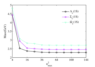
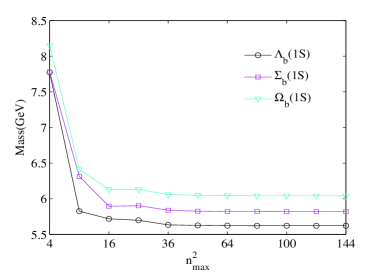
Most of the parameters used in this work are taken from the original referencequam1 b 𝑏 b c 𝑐 c 0.18 0.18 0.18 − 253 253 -253 0.14 0.14 0.14 198 198 198 Λ Q ( 1 2 + ) subscript Λ 𝑄 superscript 1 2 \Lambda_{Q}(\frac{1}{2}^{+}) Σ Q ( 1 2 + ) subscript Σ 𝑄 superscript 1 2 \Sigma_{Q}(\frac{1}{2}^{+}) Ω Q ( 1 2 + ) subscript Ω 𝑄 superscript 1 2 \Omega_{Q}(\frac{1}{2}^{+}) n m a x 2 = 10 2 superscript subscript 𝑛 𝑚 𝑎 𝑥 2 superscript 10 2 n_{max}^{2}=10^{2} 10 2 superscript 10 2 10^{2}
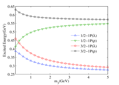
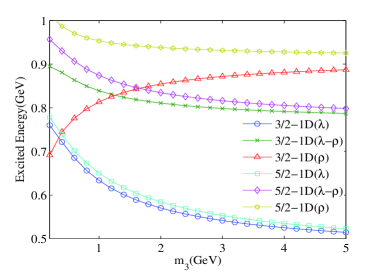
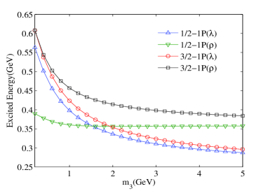
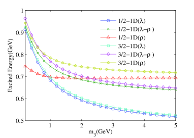
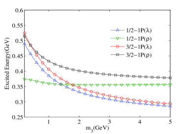
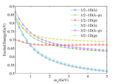
In the scheme of channel 3 3 3 l ρ subscript 𝑙 𝜌 l_{\rho} l λ subscript 𝑙 𝜆 l_{\lambda} P 𝑃 P λ 𝜆 \lambda ρ 𝜌 \rho l ρ subscript 𝑙 𝜌 l_{\rho} l λ subscript 𝑙 𝜆 l_{\lambda} 0 0 1 1 1 1 1 1 0 0 D 𝐷 D l ρ subscript 𝑙 𝜌 l_{\rho} l λ subscript 𝑙 𝜆 l_{\lambda} 0 0 2 2 2 2 2 2 0 0 1 1 1 1 1 1 λ 𝜆 \lambda ρ 𝜌 \rho λ 𝜆 \lambda ρ 𝜌 \rho D 𝐷 D m Q subscript 𝑚 𝑄 m_{Q} 0.2 0.2 0.2 5.0 5.0 5.0 Λ Q subscript Λ 𝑄 \Lambda_{Q} Σ Q subscript Σ 𝑄 \Sigma_{Q} Ω Q subscript Ω 𝑄 \Omega_{Q} m Q subscript 𝑚 𝑄 m_{Q} λ 𝜆 \lambda ρ 𝜌 \rho λ 𝜆 \lambda ρ 𝜌 \rho λ 𝜆 \lambda m Q subscript 𝑚 𝑄 m_{Q} P 𝑃 P D 𝐷 D λ 𝜆 \lambda m Q = 0.4 subscript 𝑚 𝑄 0.4 m_{Q}=0.4 Λ Q subscript Λ 𝑄 \Lambda_{Q} m Q ≥ 1.0 subscript 𝑚 𝑄 1.0 m_{Q}\geq 1.0 D 𝐷 D Σ Q subscript Σ 𝑄 \Sigma_{Q} Ω Q subscript Ω 𝑄 \Omega_{Q} P 𝑃 P Σ Q subscript Σ 𝑄 \Sigma_{Q} Ω Q subscript Ω 𝑄 \Omega_{Q} λ 𝜆 \lambda ρ 𝜌 \rho λ 𝜆 \lambda m Q ≥ 1.6 subscript 𝑚 𝑄 1.6 m_{Q}\geq 1.6
From these figures, the heavy quark spin symmetry(HQS) is also displayed. For P 𝑃 P Λ Q subscript Λ 𝑄 \Lambda_{Q} m Q subscript 𝑚 𝑄 m_{Q} 0.2 0.2 0.2 5.0 5.0 5.0 1 2 − superscript 1 2 \frac{1}{2}^{-} 3 2 − superscript 3 2 \frac{3}{2}^{-} λ 𝜆 \lambda 80 80 80 10 10 10 P 𝑃 P Λ Q subscript Λ 𝑄 \Lambda_{Q} ρ 𝜌 \rho
3.2 Mass spectra of Λ Q subscript Λ 𝑄 \Lambda_{Q} Σ Q subscript Σ 𝑄 \Sigma_{Q} Ω Q subscript Ω 𝑄 \Omega_{Q}
From these above discussions, we know that each state of the single heavy baryons is dominated and characterized by the λ 𝜆 \lambda Λ Q subscript Λ 𝑄 \Lambda_{Q} Σ Q subscript Σ 𝑄 \Sigma_{Q} Ω Q subscript Ω 𝑄 \Omega_{Q} λ 𝜆 \lambda Appendix A.1 (Tables III-VIII). In the first two columns of these tables we give the baryon quantum numbers (l ρ subscript 𝑙 𝜌 l_{\rho} l λ subscript 𝑙 𝜆 l_{\lambda} L 𝐿 L s 𝑠 s j 𝑗 j n L 𝑛 𝐿 nL J P superscript 𝐽 𝑃 J^{P}
A. Λ Q subscript Λ 𝑄 \Lambda_{Q}
It can be seen from Tables III-IV, the available experimental data for Λ Q subscript Λ 𝑄 \Lambda_{Q} Λ c ( 2765 ) subscript Λ 𝑐 2765 \Lambda_{c}(2765) Λ c ( 2940 ) subscript Λ 𝑐 2940 \Lambda_{c}(2940) Λ b ( 6070 ) subscript Λ 𝑏 6070 \Lambda_{b}(6070) article2A ; article2B S 𝑆 S 1 2 + superscript 1 2 \frac{1}{2}^{+} 2.764 2.764 2.764 Λ c ( 2765 ) subscript Λ 𝑐 2765 \Lambda_{c}(2765) Λ c ( 2765 ) subscript Λ 𝑐 2765 \Lambda_{c}(2765) S 𝑆 S 1 2 + superscript 1 2 \frac{1}{2}^{+} Λ c ( 2940 ) subscript Λ 𝑐 2940 \Lambda_{c}(2940) J P = 3 2 − superscript 𝐽 𝑃 superscript 3 2 J^{P}=\frac{3}{2}^{-} P 𝑃 P 1 2 − superscript 1 2 \frac{1}{2}^{-} P 𝑃 P 3 2 − superscript 3 2 \frac{3}{2}^{-} 2.988 2.988 2.988 3.013 3.013 3.013 P 𝑃 P 1 2 − superscript 1 2 \frac{1}{2}^{-} Λ c ( 2940 ) subscript Λ 𝑐 2940 \Lambda_{c}(2940) P 𝑃 P 3 2 − superscript 3 2 \frac{3}{2}^{-} P 𝑃 P 1 2 − superscript 1 2 \frac{1}{2}^{-} 50 50 50 quam2 Λ b ( 6070 ) subscript Λ 𝑏 6070 \Lambda_{b}(6070) S 𝑆 S 1 2 + superscript 1 2 \frac{1}{2}^{+} 60701 ; WZG2 6.041 6.041 6.041 29 29 29
Besides of these above states, some other low-lying Λ Q subscript Λ 𝑄 \Lambda_{Q} 2 P 2 𝑃 2P Λ c subscript Λ 𝑐 \Lambda_{c} 3 2 − superscript 3 2 \frac{3}{2}^{-} 1 2 − superscript 1 2 \frac{1}{2}^{-} 3 2 − superscript 3 2 \frac{3}{2}^{-} 3.013 3.013 3.013 Λ b subscript Λ 𝑏 \Lambda_{b} 2 P 2 𝑃 2P 1 2 − superscript 1 2 \frac{1}{2}^{-} 3 2 − superscript 3 2 \frac{3}{2}^{-} Λ c subscript Λ 𝑐 \Lambda_{c} 6.238 6.238 6.238 6.249 6.249 6.249
B. Σ Q subscript Σ 𝑄 \Sigma_{Q}
The lowest states of S 𝑆 S Σ c subscript Σ 𝑐 \Sigma_{c} Σ b subscript Σ 𝑏 \Sigma_{b} J P = 1 2 + superscript 𝐽 𝑃 superscript 1 2 J^{P}=\frac{1}{2}^{+} J P = 3 2 + superscript 𝐽 𝑃 superscript 3 2 J^{P}=\frac{3}{2}^{+} article2A S 𝑆 S Σ Q subscript Σ 𝑄 \Sigma_{Q} 1 2 − superscript 1 2 \frac{1}{2}^{-} 3 2 − superscript 3 2 \frac{3}{2}^{-} 3 2 − superscript 3 2 \frac{3}{2}^{-} 5 2 − superscript 5 2 \frac{5}{2}^{-} 1 2 − superscript 1 2 \frac{1}{2}^{-} 1 P 1 𝑃 1P Σ Q subscript Σ 𝑄 \Sigma_{Q} Σ c ( 2800 ) subscript Σ 𝑐 2800 \Sigma_{c}(2800) Σ b ( 6097 ) subscript Σ 𝑏 6097 \Sigma_{b}(6097) P 𝑃 P P 𝑃 P Σ c ( 2800 ) subscript Σ 𝑐 2800 \Sigma_{c}(2800) Σ b ( 6097 ) subscript Σ 𝑏 6097 \Sigma_{b}(6097) Σ c ( 2800 ) subscript Σ 𝑐 2800 \Sigma_{c}(2800) 1 P 1 𝑃 1P 1 2 − superscript 1 2 \frac{1}{2}^{-} j=1 2.809 2.809 2.809 1 P 1 𝑃 1P 3 2 − superscript 3 2 \frac{3}{2}^{-} j=2 2.802 2.802 2.802 Σ b subscript Σ 𝑏 \Sigma_{b} 1 P 1 𝑃 1P 1 2 − superscript 1 2 \frac{1}{2}^{-} j=1 1 P 1 𝑃 1P 3 2 − superscript 3 2 \frac{3}{2}^{-} j=2 6.107 6.107 6.107 6.104 6.104 6.104 Σ b ( 6097 ) subscript Σ 𝑏 6097 \Sigma_{b}(6097) Σ c ( 2800 ) subscript Σ 𝑐 2800 \Sigma_{c}(2800) Σ b ( 6097 ) subscript Σ 𝑏 6097 \Sigma_{b}(6097) P 𝑃 P Σ Q subscript Σ 𝑄 \Sigma_{Q}
It can be seen from Tables V-VI, more efforts are needed in searching for Σ Q subscript Σ 𝑄 \Sigma_{Q} Σ c ( 2800 ) subscript Σ 𝑐 2800 \Sigma_{c}(2800) Σ b ( 6097 ) subscript Σ 𝑏 6097 \Sigma_{b}(6097) 1 P 1 𝑃 1P 1 P 1 𝑃 1P 2 S 2 𝑆 2S 100 100 100 1 P 1 𝑃 1P 30 30 30 2 S 2 𝑆 2S 1 P 1 𝑃 1P Σ Q subscript Σ 𝑄 \Sigma_{Q} 1 D 1 𝐷 1D Σ Q subscript Σ 𝑄 \Sigma_{Q} 3.072 3.072 3.072 3.084 3.084 3.084 1 D 1 𝐷 1D Σ c subscript Σ 𝑐 \Sigma_{c} 6.338 6.338 6.338 6.346 6.346 6.346 Σ b subscript Σ 𝑏 \Sigma_{b}
C. Ω Q subscript Ω 𝑄 \Omega_{Q}
For Ω Q subscript Ω 𝑄 \Omega_{Q} S 𝑆 S Ω c subscript Ω 𝑐 \Omega_{c} 1 2 + superscript 1 2 \frac{1}{2}^{+} 3 2 + superscript 3 2 \frac{3}{2}^{+} 1 S 1 𝑆 1S Ω b subscript Ω 𝑏 \Omega_{b} 1 2 + superscript 1 2 \frac{1}{2}^{+} article2A Ω Q subscript Ω 𝑄 \Omega_{Q} 1 S 1 𝑆 1S 3 2 + superscript 3 2 \frac{3}{2}^{+} Ω b subscript Ω 𝑏 \Omega_{b} 6.069 6.069 6.069 Ω c subscript Ω 𝑐 \Omega_{c} Ω b subscript Ω 𝑏 \Omega_{b} Ω c ( 3000 ) subscript Ω 𝑐 3000 \Omega_{c}(3000) Ω c ( 3050 ) subscript Ω 𝑐 3050 \Omega_{c}(3050) Ω c ( 3066 ) subscript Ω 𝑐 3066 \Omega_{c}(3066) Ω c ( 3090 ) subscript Ω 𝑐 3090 \Omega_{c}(3090) Ω c ( 3119 ) subscript Ω 𝑐 3119 \Omega_{c}(3119) OmegaC3000 Ω b ( 6316 ) subscript Ω 𝑏 6316 \Omega_{b}(6316) Ω b ( 6330 ) subscript Ω 𝑏 6330 \Omega_{b}(6330) Ω b ( 6340 ) subscript Ω 𝑏 6340 \Omega_{b}(6340) Ω b ( 6350 ) subscript Ω 𝑏 6350 \Omega_{b}(6350) OmegaB6316 Ω c subscript Ω 𝑐 \Omega_{c} 2 S 2 𝑆 2S 1 2 + superscript 1 2 \frac{1}{2}^{+} 3.150 3.150 3.150 Ω c ( 3119 ) subscript Ω 𝑐 3119 \Omega_{c}(3119) Ω c ( 3119 ) subscript Ω 𝑐 3119 \Omega_{c}(3119) 2 S 2 𝑆 2S 1 2 + superscript 1 2 \frac{1}{2}^{+} Ω c subscript Ω 𝑐 \Omega_{c} P 𝑃 P 1 P 1 𝑃 1P Ω c subscript Ω 𝑐 \Omega_{c} 1 2 − superscript 1 2 \frac{1}{2}^{-} 3 2 − superscript 3 2 \frac{3}{2}^{-} 3 2 − superscript 3 2 \frac{3}{2}^{-} 5 2 − superscript 5 2 \frac{5}{2}^{-} 17 17 17 28 28 28 Ω c subscript Ω 𝑐 \Omega_{c} Ω c ( 3000 ) subscript Ω 𝑐 3000 \Omega_{c}(3000) Ω c ( 3050 ) subscript Ω 𝑐 3050 \Omega_{c}(3050) = = 1 2 − superscript 1 2 \frac{1}{2}^{-} 3 2 − superscript 3 2 \frac{3}{2}^{-} j=1 Ω c ( 3066 ) subscript Ω 𝑐 3066 \Omega_{c}(3066) Ω c ( 3090 ) subscript Ω 𝑐 3090 \Omega_{c}(3090) 3 2 − superscript 3 2 \frac{3}{2}^{-} 5 2 − superscript 5 2 \frac{5}{2}^{-} j=2 Ω b subscript Ω 𝑏 \Omega_{b} 1 P 1 𝑃 1P Ω c subscript Ω 𝑐 \Omega_{c} 1 2 − superscript 1 2 \frac{1}{2}^{-} 3 2 − superscript 3 2 \frac{3}{2}^{-} j=1 3 2 − superscript 3 2 \frac{3}{2}^{-} 5 2 − superscript 5 2 \frac{5}{2}^{-} j=2 7 7 7 13 13 13 Ω b subscript Ω 𝑏 \Omega_{b} P 𝑃 P Ω b ( 6315 ) subscript Ω 𝑏 6315 \Omega_{b}(6315) Ω b ( 6330 ) subscript Ω 𝑏 6330 \Omega_{b}(6330) = = 1 2 − superscript 1 2 \frac{1}{2}^{-} 3 2 − superscript 3 2 \frac{3}{2}^{-} j=1 Ω b ( 6340 ) subscript Ω 𝑏 6340 \Omega_{b}(6340) Ω b ( 6350 ) subscript Ω 𝑏 6350 \Omega_{b}(6350) 3 2 − superscript 3 2 \frac{3}{2}^{-} 5 2 − superscript 5 2 \frac{5}{2}^{-} j=2 Ω c subscript Ω 𝑐 \Omega_{c} Ω b subscript Ω 𝑏 \Omega_{b} OmegaC30001 ; OmegaC30002 ; OmegaC30003 ; OmegaC30004 ; OmegaC30005 ; OmegaC30006 ; OmegaC30007 ; OmegaB63301 ; OmegaB63302 ; OmegaB63303 P 𝑃 P Ω Q subscript Ω 𝑄 \Omega_{Q}
In quark model scheme, there are two 2 S 2 𝑆 2S 6.446 6.446 6.446 6.466 6.466 6.466 quam2 Ω b subscript Ω 𝑏 \Omega_{b} 1 D 1 𝐷 1D Ω Q subscript Ω 𝑄 \Omega_{Q} 3.304 3.304 3.304 ∼ similar-to \sim 3.315 3.315 3.315 Ω c subscript Ω 𝑐 \Omega_{c} 1 D 1 𝐷 1D 6.555 6.555 6.555 ∼ similar-to \sim 6.562 6.562 6.562 Ω b subscript Ω 𝑏 \Omega_{b} 1 D 1 𝐷 1D
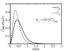
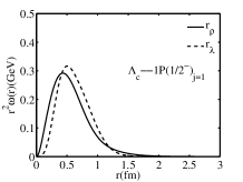
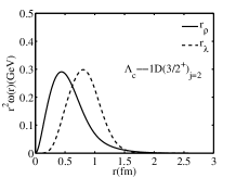
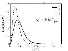
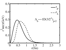
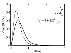
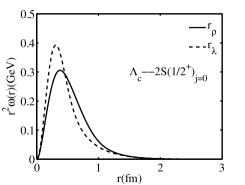
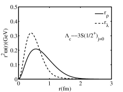
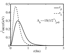
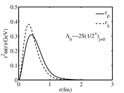
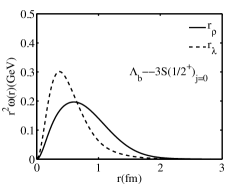
3.3 Root mean square radius and radial density distributions
Besides of the root mean square radius, we also calculated the radial density distributions which are defined as,
ω ( r ρ ) = ∫ | Ψ ( r ρ , r λ ) | 2 𝑑 r λ 𝑑 Ω ρ 𝜔 subscript 𝑟 𝜌 superscript Ψ subscript r 𝜌 subscript r 𝜆 2 differential-d subscript r 𝜆 differential-d subscript Ω 𝜌 \displaystyle\omega(r_{\rho})=\int|\Psi(\textbf{r}_{\rho},\textbf{r}_{\lambda})|^{2}d\textbf{r}_{\lambda}d\Omega_{\rho}
ω ( r λ ) = ∫ | Ψ ( r ρ , r λ ) | 2 𝑑 r ρ 𝑑 Ω λ 𝜔 subscript 𝑟 𝜆 superscript Ψ subscript r 𝜌 subscript r 𝜆 2 differential-d subscript r 𝜌 differential-d subscript Ω 𝜆 \displaystyle\omega(r_{\lambda})=\int|\Psi(\textbf{r}_{\rho},\textbf{r}_{\lambda})|^{2}d\textbf{r}_{\rho}d\Omega_{\lambda} (42)
where Ω ρ subscript Ω 𝜌 \Omega_{\rho} Ω λ subscript Ω 𝜆 \Omega_{\lambda} r ρ subscript r 𝜌 \textbf{r}_{\rho} r λ subscript r 𝜆 \textbf{r}_{\lambda} Λ Q subscript Λ 𝑄 \Lambda_{Q}
Figure 10: Radial density distributions for some 1 S − 1 F 1 𝑆 1 𝐹 1S-1F Λ c subscript Λ 𝑐 \Lambda_{c}
Figure 11: Radial density distributions for some 1 S − 1 F 1 𝑆 1 𝐹 1S-1F Λ b subscript Λ 𝑏 \Lambda_{b}
Figure 12: Radial density distributions for 1 S ∼ 3 S similar-to 1 𝑆 3 𝑆 1S\sim 3S Λ c subscript Λ 𝑐 \Lambda_{c}
Figure 13: Radial density distributions for 1 S ∼ 3 S similar-to 1 𝑆 3 𝑆 1S\sim 3S Λ b subscript Λ 𝑏 \Lambda_{b}
From Tables III-VIII, we can see the root mean square radius ⟨ r ρ ⟩ 1 2 subscript delimited-⟨⟩ subscript 𝑟 𝜌 1 2 \langle r_{\rho}\rangle_{\frac{1}{2}} ⟨ r λ ⟩ 1 2 subscript delimited-⟨⟩ subscript 𝑟 𝜆 1 2 \langle r_{\lambda}\rangle_{\frac{1}{2}} 1 S 1 𝑆 1S ∼ similar-to \sim ∼ similar-to \sim n 𝑛 n ⟨ r λ ⟩ 1 2 subscript delimited-⟨⟩ subscript 𝑟 𝜆 1 2 \langle r_{\lambda}\rangle_{\frac{1}{2}} L 𝐿 L ⟨ r ρ ⟩ 1 2 subscript delimited-⟨⟩ subscript 𝑟 𝜌 1 2 \langle r_{\rho}\rangle_{\frac{1}{2}} ω ( r λ ) 𝜔 subscript 𝑟 𝜆 \omega(r_{\lambda}) L 𝐿 L ω ( r ρ ) 𝜔 subscript 𝑟 𝜌 \omega(r_{\rho}) L 𝐿 L ⟨ r ρ ⟩ 1 2 subscript delimited-⟨⟩ subscript 𝑟 𝜌 1 2 \langle r_{\rho}\rangle_{\frac{1}{2}} ⟨ r λ ⟩ 1 2 subscript delimited-⟨⟩ subscript 𝑟 𝜆 1 2 \langle r_{\lambda}\rangle_{\frac{1}{2}} n 𝑛 n
It is known that the larger the root mean square radius become, the looser the baryons will be. We can see from Tables III-VIII, the mean square radius of the experimentally established baryons are almost less than 0.8 fm. If we roughly take this value as a criterion, all of the predicted states with radius less than 0.8 fm have potentials to be discovered in forthcoming experiments.
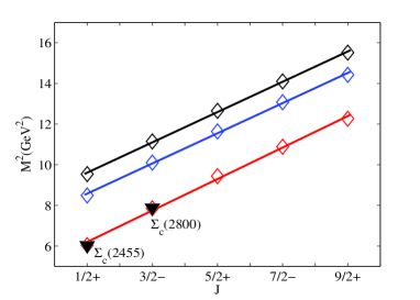
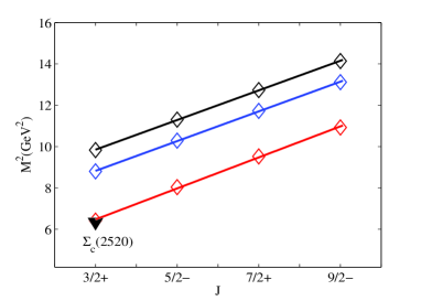
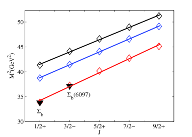
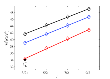
4 Regge trajectories of single heavy baryons Λ Q subscript Λ 𝑄 \Lambda_{Q} Σ Q subscript Σ 𝑄 \Sigma_{Q} Ω Q subscript Ω 𝑄 \Omega_{Q}
The well-known Regge theory was first developed by T.Regge in 1959Regge1 ; Regge2 J 𝐽 J M 2 superscript 𝑀 2 M^{2} Regge3 ; Regge4 J 𝐽 J M 𝑀 M Regge5 ; Regge6 ; Regge7 ; Regge8 Regge9 ; Regge10 J 𝐽 J M 2 superscript 𝑀 2 M^{2}
J = M 2 2 π σ + c 𝐽 superscript 𝑀 2 2 𝜋 𝜎 𝑐 \displaystyle J=\frac{M^{2}}{2\pi\sigma}+c (43)
where, σ 𝜎 \sigma c 𝑐 c
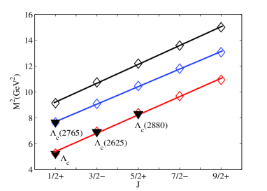
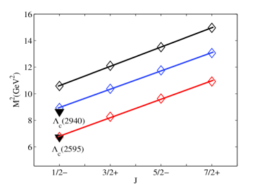
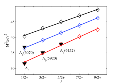
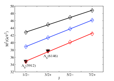
In the present work, we obtained the masses of both orbitally and radially excited charmed and bottom baryons up to rather high excitation numbers, which makes it easy for us to construct the baryon Regge trajectories in (J 𝐽 J M 2 superscript 𝑀 2 M^{2} P = ( − 1 ) J − 1 / 2 𝑃 superscript 1 𝐽 1 2 P=(-1)^{J-1/2} P = ( − 1 ) J + 1 / 2 𝑃 superscript 1 𝐽 1 2 P=(-1)^{J+1/2} quam2 J 𝐽 J M 2 superscript 𝑀 2 M^{2} Λ Q subscript Λ 𝑄 \Lambda_{Q} Σ Q subscript Σ 𝑄 \Sigma_{Q} Ω Q subscript Ω 𝑄 \Omega_{Q} J 𝐽 J M 2 superscript 𝑀 2 M^{2} quam2
J = α M 2 + α 0 𝐽 𝛼 superscript 𝑀 2 subscript 𝛼 0 \displaystyle J=\alpha M^{2}+\alpha_{0} (44)
where α 𝛼 \alpha α 0 subscript 𝛼 0 \alpha_{0} Appendix A.2 (Table IX).
Figure 14: Parent and daughter (J 𝐽 J M 2 superscript 𝑀 2 M^{2} Λ c subscript Λ 𝑐 \Lambda_{c}
Figure 15: Same as in FIG.10 for the Λ b subscript Λ 𝑏 \Lambda_{b}
Figure 16: Same as in FIG.10 for the Σ c subscript Σ 𝑐 \Sigma_{c}
Figure 17: Same as in FIG.10 for the Σ b subscript Σ 𝑏 \Sigma_{b}
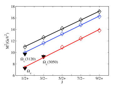
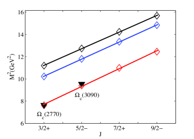
Figure 18: Same as in FIG.10 for the Ω c subscript Ω 𝑐 \Omega_{c}
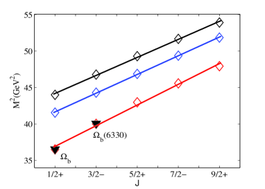
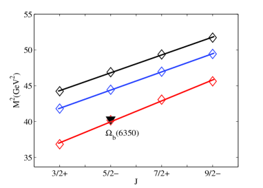
Figure 19: Same as in FIG.10 for the Ω b subscript Ω 𝑏 \Omega_{b}
We can see from these figures that all of the predicted masses in our model fit nicely to the linear trajectories in the (J 𝐽 J M 2 superscript 𝑀 2 M^{2} Λ c ( 1 2 + ) subscript Λ 𝑐 superscript 1 2 \Lambda_{c}(\frac{1}{2}^{+}) Λ b ( 1 2 + ) subscript Λ 𝑏 superscript 1 2 \Lambda_{b}(\frac{1}{2}^{+}) Λ c ( 1 2 − ) subscript Λ 𝑐 superscript 1 2 \Lambda_{c}(\frac{1}{2}^{-}) Σ c ( 2455 ) ( 1 2 + ) subscript Σ 𝑐 2455 superscript 1 2 \Sigma_{c}(2455)(\frac{1}{2}^{+}) Σ b ( 1 2 + ) subscript Σ 𝑏 superscript 1 2 \Sigma_{b}(\frac{1}{2}^{+}) Ω c ( 1 2 + ) subscript Ω 𝑐 superscript 1 2 \Omega_{c}(\frac{1}{2}^{+}) Ω c ( 2770 ) ( 3 2 + ) subscript Ω 𝑐 2770 superscript 3 2 \Omega_{c}(2770)(\frac{3}{2}^{+}) Ω b ( 1 2 + ) subscript Ω 𝑏 superscript 1 2 \Omega_{b}(\frac{1}{2}^{+}) Λ c ( 2765 ) subscript Λ 𝑐 2765 \Lambda_{c}(2765) Λ b ( 6070 ) subscript Λ 𝑏 6070 \Lambda_{b}(6070) 2 S 2 𝑆 2S 1 2 + superscript 1 2 \frac{1}{2}^{+} Λ c ( 2940 ) subscript Λ 𝑐 2940 \Lambda_{c}(2940) 2 P 2 𝑃 2P 1 2 − superscript 1 2 \frac{1}{2}^{-} 40 ∼ 50 similar-to 40 50 40\sim 50 Σ c ( 2800 ) subscript Σ 𝑐 2800 \Sigma_{c}(2800) Σ b ( 6097 ) subscript Σ 𝑏 6097 \Sigma_{b}(6097) 1 P 1 𝑃 1P 3 2 − superscript 3 2 \frac{3}{2}^{-} Ω c ( 3120 ) subscript Ω 𝑐 3120 \Omega_{c}(3120) 2 S 2 𝑆 2S Ω c subscript Ω 𝑐 \Omega_{c} 1 2 + superscript 1 2 \frac{1}{2}^{+} Ω c subscript Ω 𝑐 \Omega_{c} Ω c ( 3050 ) subscript Ω 𝑐 3050 \Omega_{c}(3050) Ω c ( 3090 ) subscript Ω 𝑐 3090 \Omega_{c}(3090) 1 P 1 𝑃 1P 3 2 − superscript 3 2 \frac{3}{2}^{-} 5 2 − superscript 5 2 \frac{5}{2}^{-} Ω b ( 6330 ) subscript Ω 𝑏 6330 \Omega_{b}(6330) Ω b ( 6350 ) subscript Ω 𝑏 6350 \Omega_{b}(6350) Ω c subscript Ω 𝑐 \Omega_{c} 1 P 1 𝑃 1P Ω c subscript Ω 𝑐 \Omega_{c} J P = 3 2 − superscript 𝐽 𝑃 superscript 3 2 J^{P}=\frac{3}{2}^{-} 5 2 − superscript 5 2 \frac{5}{2}^{-}
In this work, we have systematically investigate the mass spectra of the single heavy baryons Λ Q subscript Λ 𝑄 \Lambda_{Q} Σ Q subscript Σ 𝑄 \Sigma_{Q} Ω Q subscript Ω 𝑄 \Omega_{Q} J 𝐽 J M 2 superscript 𝑀 2 M^{2}
(1)We have studied the dependencies on the heavy quark mass m Q subscript 𝑚 𝑄 m_{Q} λ 𝜆 \lambda ρ 𝜌 \rho λ 𝜆 \lambda ρ 𝜌 \rho λ 𝜆 \lambda Λ Q subscript Λ 𝑄 \Lambda_{Q} Σ Q subscript Σ 𝑄 \Sigma_{Q} Ω Q subscript Ω 𝑄 \Omega_{Q} λ 𝜆 \lambda
(2)We also investigate the root mean square radius and the radial density distributions of the single heavy baryons. We hope these analysis can help us to predict the upper limit of the mass spectra and to search for baryons which have potentials to be found in experiments.
(3)With the predicted masses, we construct the Regge trajectories in (J 𝐽 J M 2 superscript 𝑀 2 M^{2} J 𝐽 J M 2 superscript 𝑀 2 M^{2}
(4)According to the predicted mass spectra, a number of experimental states without spin-parity assignments are successfully distinguished and a number of single heavy barons which have good potentials to be discovered in forthcoming experiments are predicted by quark model.
References
(1)
H. Albrecht e t 𝑒 𝑡 et a l 𝑎 𝑙 al
(2)
P. L. Frabetti e t 𝑒 𝑡 et a l 𝑎 𝑙 al
(3)
R. Aaij e t 𝑒 𝑡 et a l 𝑎 𝑙 al
(4)
T. A. Aaltonen e t 𝑒 𝑡 et a l 𝑎 𝑙 al
(5)
P. A. Zyla e t 𝑒 𝑡 et a l 𝑎 𝑙 al
(6)
K. Nakamura e t 𝑒 𝑡 et a l 𝑎 𝑙 al
(7)
A. Abdesselam e t 𝑒 𝑡 et a l 𝑎 𝑙 al
(8)
B. Aubert e t 𝑒 𝑡 et a l 𝑎 𝑙 al
(9)
K. Abe e t 𝑒 𝑡 et a l 𝑎 𝑙 al
(10)
R. Aaij e t 𝑒 𝑡 et a l 𝑎 𝑙 al
(11)
R. Aaij e t 𝑒 𝑡 et a l 𝑎 𝑙 al
(12)
R. Aaij e t 𝑒 𝑡 et a l 𝑎 𝑙 al
(13)
R. Mizuke t 𝑒 𝑡 et a l 𝑎 𝑙 al
(14)
R. Aaij e t 𝑒 𝑡 et a l 𝑎 𝑙 al
(15)
R. Aaij e t 𝑒 𝑡 et a l 𝑎 𝑙 al
(16)
R. Aaij e t 𝑒 𝑡 et a l 𝑎 𝑙 al
(17)
S. Godfrey and N. Isgur, Phys. Rev. D 32, 189(1985).
(18)
S. Capstick and N. Isgur, Phys. Rev. D 34, 2809 (1986); AIPConf. Proc. 132, 267(1985).
(19)
D. Ebert, R. N. Faustov, and V. O. Galkin, Phys. Rev. D 84, 014025(2011).
(20)
W. Roberts and M. Pervin, Int. J. Mod. Phys. A 23, 2817(2008).
(21)
T. Yoshida, E. Hiyama, A. Hosaka, e t 𝑒 𝑡 et a l 𝑎 𝑙 al
(22)
K. L. Wang, Q. F. Lü, and X. H. Zhong, Phys. Rev. D 100, 114035(2019).
(23)
L. A. Copley, N. Isgur, and G. Karl, Phys. Rev. D 20, 768(1979); 23, 817(E)(1981).
(24)
K. Maltman and N. Isgur, Phys. Rev. D 22, 1701(1980).
(25)
D. Ebert, R. N. Faustov, and V. O. Galkin, Phys. Rev. D 72, 034026(2005).
(26)
D. Ebert, R. N. Faustov, and V. O. Galkin, Phys. Lett. B 659, 612(2008).
(27)
H. Garcilazo, J. Vijande, and A. Valcarce, J. Phys. G 34, 961(2007).
(28)
M. Karliner and J. L. Rosner, Phys. Rev. D 92, 074026(2015).
(29)
K. Thakkar, Z. Shah, A. K. Rai, e t 𝑒 𝑡 et a l 𝑎 𝑙 al
(30)
Z. Shah, K. Thakkar, A. K. Rai, e t 𝑒 𝑡 et a l 𝑎 𝑙 al
(31)
Z. Shah, K. Thakkar, A. Kumar Rai, e t 𝑒 𝑡 et a l 𝑎 𝑙 al
(32)
F. Hussain, J. G. Korner, and S. Tawfiq, Phys. Rev. D 61, 114003(2000).
(33)
M. A. Ivanov, J. G. Korner, and V. E. Lyubovitskij, Phys.Lett. B 448, 143(1999).
(34)
M. A. Ivanov, J. G. Korner, V. E. Lyubovitskij, e t 𝑒 𝑡 et a l 𝑎 𝑙 al
(35)
C. Albertus, E. Hernandez, J. Nieves, e t 𝑒 𝑡 et a l 𝑎 𝑙 al
(36)
S. Migura, D. Merten, B. Metsch, e t 𝑒 𝑡 et a l 𝑎 𝑙 al
(37)
X. H. Zhong and Q. Zhao, Phys. Rev. D 77, 074008(2008).
(38)
E. Hernandez and J. Nieves, Phys. Rev. D 84, 057902(2011).
(39)
L. H. Liu, L. Y. Xiao, and X. H. Zhong, Phys. Rev. D 86, 034024(2012).
(40)
B. Chen, K. W. Wei, X. Liu, and T. Matsuki, Eur. Phys. J. C 77, 154(2017).
(41)
B. Chen and X. Liu, Phys. Rev. D 98, 074032(2018).
(42)
H. Nagahiro, S. Yasui, A. Hosaka, M. Oka, and H. Noumi, Phys. Rev. D 95, 014023(2017).
(43)
Y. X. Yao, K. L. Wang, and X. H. Zhong, Phys. Rev. D 98, 076015(2018).
(44)
A. Valcarce, H. Garcilazo, and J. Vijande, Eur. Phys. J. A37, 217(2008).
(45)
M. Q. Huang, Y. B. Dai, and C. S. Huang, Phys. Rev. D 52, 3986(1995); 55, 7317(E)(1997).
(46)
M. C. Banuls, A. Pich, and I. Scimemi, Phys. Rev. D 61, 094009(2000).
(47)
H. Y. Cheng and C. K. Chua, Phys. Rev. D 75, 014006(2007).
(48)
N. Jiang, X. L. Chen, and S. L. Zhu, Phys. Rev. D 92, 054017(2015).
(49)
H. Y. Cheng and C. K. Chua, Phys. Rev. D 92, 074014(2015).
(50)
Y. Kawakami and M. Harada, Phys. Rev. D 99, 094016(2019).
(51)
M. Padmanath, R. G. Edwards, N. Mathur, and M. Peardon, arXiv:1311.4806(2013).
(52)
H. Bahtiyar, K. U. Can, G. Erkol, and M. Oka, Phys. Lett. B747, 281(2015).
(53)
P. Perez-Rubio, S. Collins, and G. S. Bali, Phys. Rev. D 92,034504(2015).
(54)
H. Bahtiyar, K. U. Can, G. Erkol, M. Oka, and T. T.Takahashi, Phys. Lett. B 772, 121(2017).
(55)
S. L. Zhu and Y. B. Dai, Phys. Rev. D 59, 114015(1999).
(56)
S. S. Agaev, K. Azizi, and H. Sundu, Phys. Rev. D 96, 094011(2017).
(57)
H. X. Chen, Q. Mao, W. Chen, A. Hosaka, X. Liu, and S. L.Zhu, Phys. Rev. D 95, 094008(2017).
(58)
Z. G. Wang, Phys. Rev. D 81, 036002(2010).
(59)
Z. G. Wang, Eur. Phys. J. A 44, 105(2010).
(60)
T. M. Aliev, K. Azizi, and H. Sundu, Eur. Phys. J. C 75, 14(2015).
(61)
T. M. Aliev, T. Barakat, and M. Savci, Phys. Rev. D 93, 056007(2016).
(62)
T. M. Aliev, K. Azizi, Y. Sarac, and H. Sundu, Phys. Rev. D 99, 094003(2019).
(63)
S. L. Zhu, Phys. Rev. D 61, 114019(2000).
(64)
Z. G. Wang, Eur. Phys. J. A 47, 81(2011).
(65)
Q. Mao, H. X. Chen, W. Chen, A. Hosaka, X. Liu, and S. L.Zhu, Phys. Rev. D 92, 114007(2015).
(66)
H. X. Chen, Q. Mao, A. Hosaka, X. Liu, and S. L. Zhu,Phys. Rev. D 94, 114016(2016).
(67)
Z. G. Wang, Nucl. Phys. B 926, 467(2018).
(68)
Q. Mao, H. X. Chen, A. Hosaka, X. Liu, and S. L. Zhu,Phys. Rev. D 96, 074021(2017).
(69)
T. M. Aliev, K. Azizi, Y. Sarac, and H. Sundu, Phys. Rev. D 98, 094014(2018).
(70)
E. L. Cui, H. M. Yang, H. X. Chen, and A. Hosaka, Phys.Rev. D 99, 094021(2019).
(71)
K. Azizi, Y. Sarac, and H. Sundu, Phys. Rev. D 101, 074026(2020).
(72)
X. Liu, H. X. Chen, Y. R. Liu, A. Hosaka and S. L. Zhu, Phys. Rev. D 77, 014031(2008).
(73)
Francisco O. Duraes, Marina Nielsen, Phys. Lett. B 658, 40(2007).
(74)
J. R. Zhang, M. Q. Huang, Phys. Rev. D 77, 094002(2008).
(75)
J. R. Zhang, M. Q. Huang, Phys. Rev. D 78, 094015(2008).
(76)
Z. G. Wang, Chin. Phys. C 45, 013109(2021).
(77)
Z. G. Wang, Eur. Phys. J. C 68, 479(2010).
(78)
Z. G. Wang, Eur. Phys. J. C 75, 359(2015).
(79)
Z. G. Wang, Phys. Lett. B 685, 59(2010).
(80)
Z. G. Wang, Eur. Phys. J. C 77, 325(2017).
(81)
Z. G. Wang, Int. J. Mod. Phys. A 35, 2050043(2020).
(82)
G. L. Yu, Z. G. Wang, arXiv:2109.02217(2021).
(83)
B. Chen, K.W. Wei and A. Zhang, Eur. Phys. J. A 51, 82(2015).
(84)
Q. F. Lü, D. Y. Chen, and Y. B. Dong, Eur. Phys. J. C 80, 871 (2020).
(85)
Q. F. Lü, D. Y. Chen, and Y. B. Dong, e t 𝑒 𝑡 et a l 𝑎 𝑙 al
(86)
Q. F. Lü, D. Y. Chen, and Y. B. Dong, Phys. Rev. D 102, 074021 (2020)
(87)
E. Hiyama, Y. Kin, and M. Kamimura, Prog. Part. Nucl. Phys. 51, 223(2003)
(88)
K. Azizi, Y. Sarac, H. Sundu, Phys. Rev. D 102, 034007(2020).
(89)
Y. Huang, C.J. Xiao, L.S. Geng, e t 𝑒 𝑡 et a l 𝑎 𝑙 al
(90)
R. Aaij et al.(LHCb Collaboration), Phys. Rev. Lett. 122, 012001(2019).
(91)
Z. Zhao, D. D. Ye, A. Zhang, Phys. Rev. D 95, 114024 (2017).
(92)
B. Chen, X. Liu, Phys. Rev. D 96, 094015 (2017).
(93)
M. Padmanath, Nilmani Mathur, Phys. Rev. Lett. 119, 042001 (2017).
(94)
K. L. Wang, L. Y. Xiao, X. H. Zhong, e t 𝑒 𝑡 et a l 𝑎 𝑙 al
(95)
H. X. Chen, Q. Mao, W. Chen, e t 𝑒 𝑡 et a l 𝑎 𝑙 al
(96)
G. Yang, J. L. Ping, Phys. Rev. D 97, 034023 (2018).
(97)
H. M. Yang, H. X. Chen, Phys. Rev. D 104, 034037 (2021).
(98)
W. Liang, Q. F. Lü, arXiv:2001.02221(2020).
(99)
L. Y. Xiao, K. L. Wang, M. S. Liu, e t 𝑒 𝑡 et a l 𝑎 𝑙 al
(100)
Halil Mutuk, Eur. Phys. J. A 56, 146 (2020).
(101)
T. Regge, Nuovo Cim. 14, 951(1959).
(102)
T. Regge, Nuovo Cim. 18, 947(1960).
(103)
G. F. Chew, S. C. Frautschi, Phys. Rev. Lett. 7, 394(1961).
(104)
G. F. Chew, S. C. Frautschi, Phys. Rev. Lett. 8, 41 (1962).
(105)
G. S. Bali, Phys. Rept. 343, 1, arXiv:hep-ph/0001312(2001).
(106)
D. V. Bugg, Four sorts of meson, Phys. Rept. 397, 257, arXiv:hep-ex/0412045(2004).
(107)
E. Klempt, A. Zaitsev, Phys. Rept. 454, 1, arXiv:0708.4016(2007).
(108)
W. Lucha, F. F. Schoberl, D. Gromes, Phys. Rept. 200, 127(1991).
(109)
Y. Nambu, Phys. Rev. D 10, 4262(1974).
(110)
Y. Nambu, Phys. Lett. B 80, 372(1979).
(111)
K. L. Wang, Q. F. Lü and X. H. Zhong, Rev. D 99, 014011 (2019).
(112)
B. Chen, S. Q. Luo, X. Liu, e t 𝑒 𝑡 et a l 𝑎 𝑙 al
(113)
Q. F. Lü, L. Y. Xiao, Z. Y. Wang and X. H. Zhong, Eur. Phys. J. C 78,599(2018).
(114)
W. Liang, Q. F. Lü and X. H. Zhong, Phys. Rev. D 100, 054013(2019).
(115)
Q. F. Lü and X. H. Zhong, arXiv:1910.06126(2019).
(116)
S. Godfrey and K. Moats, Phys. Rev. D 93, 034035(2016).
(117)
S. Godfrey, K. Moats, and E. S. Swanson, Phys. Rev. D 94, 054025(2016).
(118)
W. Liang, Q. F. Lü, arXiv:2004.13568(2020).
(119)
H. M. Yang, H. X. Chen, Phys. Rev. D 104, 034037(2021).
(120)
K. L. Wang, Y. X. Yao, X. H. Zhong, e t 𝑒 𝑡 et a l 𝑎 𝑙 al
(121)
H. X. Chen, Q. Mao, W. Chen, e t 𝑒 𝑡 et a l 𝑎 𝑙 al
A.1 The mass spectra and root mean square radius
Table 3: The root mean square radius (fm) and the mass spectrum (MeV) of the Λ c subscript Λ 𝑐 \Lambda_{c}
Table 4: The root mean square radius (fm) and the mass spectrum (MeV) of the Λ b subscript Λ 𝑏 \Lambda_{b}
Table 5: The root mean square radius (fm) and the mass spectrum (MeV) of the Σ c subscript Σ 𝑐 \Sigma_{c}
Table 6: The root mean square radius (fm) and the mass spectrum (MeV) of the Σ b subscript Σ 𝑏 \Sigma_{b}
Table 7: The root mean square radius (fm) and the mass spectrum (MeV) of the Ω c subscript Ω 𝑐 \Omega_{c}
Table 8: The root mean square radius (fm) and the mass spectrum (MeV) of the Ω b subscript Ω 𝑏 \Omega_{b}
A.2 Fitted parameters of the Regge trajectories
Table 9: Fitted parameters α 𝛼 \alpha α 0 subscript 𝛼 0 \alpha_{0} J 𝐽 J M 2 superscript 𝑀 2 M^{2} Λ Q subscript Λ 𝑄 \Lambda_{Q} Σ Q subscript Σ 𝑄 \Sigma_{Q} Ω Q subscript Ω 𝑄 \Omega_{Q}
The coefficient C l m , k subscript 𝐶 𝑙 𝑚 𝑘
C_{lm,k} D l m , k subscript D 𝑙 𝑚 𝑘
\textbf{D}_{lm,k} ν n subscript 𝜈 𝑛 \nu_{n} ϵ italic-ϵ \epsilon
C l m , k ≡ ∑ j = 0 [ l − m 2 ] A l m , j ∑ s = 0 p ∑ t = 0 q ∑ u = 0 j ( − 1 ) l − u − t − s ( p s ) ( q t ) ( j u ) subscript 𝐶 𝑙 𝑚 𝑘
superscript subscript 𝑗 0 delimited-[] 𝑙 𝑚 2 subscript 𝐴 𝑙 𝑚 𝑗
superscript subscript 𝑠 0 𝑝 superscript subscript 𝑡 0 𝑞 superscript subscript 𝑢 0 𝑗 superscript 1 𝑙 𝑢 𝑡 𝑠 binomial 𝑝 𝑠 binomial 𝑞 𝑡 binomial 𝑗 𝑢 \displaystyle C_{lm,k}\equiv\sum_{j=0}^{\big{[}\frac{l-m}{2}\big{]}}A_{lm,j}\sum_{s=0}^{p}\sum_{t=0}^{q}\sum_{u=0}^{j}(-1)^{l-u-t-s}\binom{p}{s}\binom{q}{t}\binom{j}{u} (45)
where p = l − m − 2 j 𝑝 𝑙 𝑚 2 𝑗 p=l-m-2j q = j + m 𝑞 𝑗 𝑚 q=j+m
D l m , k ≡ 1 l [ ( 2 s − p ) a z + ( 2 t − q ) a x y + ( 2 u − j ) a x y ∗ ] subscript D 𝑙 𝑚 𝑘
1 𝑙 delimited-[] 2 𝑠 𝑝 subscript a 𝑧 2 𝑡 𝑞 subscript a 𝑥 𝑦 2 𝑢 𝑗 superscript subscript a 𝑥 𝑦 \displaystyle\textbf{D}_{lm,k}\equiv\frac{1}{l}[(2s-p)\textbf{a}_{z}+(2t-q)\textbf{a}_{xy}+(2u-j)\textbf{a}_{xy}^{*}] (46)
with
A l m , j = [ ( 2 l + 1 ) ( l − m ) ! 4 π ( l + m ) ! ] 1 2 ( l + m ) ! ( − 1 ) j ( − 2 ) m 4 j j ! ( m + j ) ! ( l − m − 2 j ) ! subscript 𝐴 𝑙 𝑚 𝑗
superscript delimited-[] 2 𝑙 1 𝑙 𝑚 4 𝜋 𝑙 𝑚 1 2 𝑙 𝑚 superscript 1 𝑗 superscript 2 𝑚 superscript 4 𝑗 𝑗 𝑚 𝑗 𝑙 𝑚 2 𝑗 \displaystyle A_{lm,j}=\Big{[}\frac{(2l+1)(l-m)!}{4\pi(l+m)!}\Big{]}^{\frac{1}{2}}\frac{(l+m)!(-1)^{j}}{(-2)^{m}4^{j}j!(m+j)!(l-m-2j)!} (47)
In Eq.(46) a z subscript a 𝑧 \textbf{a}_{z} a x y subscript a 𝑥 𝑦 \textbf{a}_{xy} a x y ∗ superscript subscript a 𝑥 𝑦 \textbf{a}_{xy}^{*} a z ≡ ( 0 , 0 , 1 ) subscript a 𝑧 0 0 1 \textbf{a}_{z}\equiv(0,0,1) a x y ≡ ( 1 , i , 0 ) subscript a 𝑥 𝑦 1 𝑖 0 \textbf{a}_{xy}\equiv(1,i,0) a x y ∗ ≡ ( 1 , − i , 0 ) superscript subscript a 𝑥 𝑦 1 𝑖 0 \textbf{a}_{xy}^{*}\equiv(1,-i,0) m < 0 𝑚 0 m<0 A l m , j → ( − 1 ) m A l − m , j → subscript 𝐴 𝑙 𝑚 𝑗
superscript 1 𝑚 subscript 𝐴 𝑙 𝑚 𝑗
A_{lm,j}\rightarrow(-1)^{m}A_{l-m,j} D → D ∗ → D superscript D \textbf{D}\rightarrow\textbf{D}^{*}
B.1 Three-body matrix elements of the potential energy
In the following, we show how to obtain matrix elements of the various pieces of the Hamiltonian in the Jacobi coordinate channel 3 3 3 H ~ i j ( r i j ) subscript ~ 𝐻 𝑖 𝑗 subscript r 𝑖 𝑗 \widetilde{H}_{ij}(\emph{{r}}_{ij}) r 12 subscript r 12 \emph{{r}}_{12} r 13 subscript r 13 \emph{{r}}_{13} r 23 subscript r 23 \emph{{r}}_{23} r 12 = r ρ 3 subscript r 12 subscript r subscript 𝜌 3 \emph{{r}}_{12}=\emph{{r}}_{\rho_{3}} r 13 = r ρ 2 subscript r 13 subscript r subscript 𝜌 2 \emph{{r}}_{13}=\emph{{r}}_{\rho_{2}} r 23 = r ρ 1 subscript r 23 subscript r subscript 𝜌 1 \emph{{r}}_{23}=\textbf{\emph{r}}_{\rho_{1}} G ~ ( 𝒓 12 ) ~ 𝐺 subscript 𝒓 12 \widetilde{G}(\boldsymbol{r}_{12})
⟨ [ ϕ n ρ a l ρ a m l ρ a ( 𝒓 ρ 3 ) ϕ n λ a l λ a m l λ a ( 𝒓 λ 3 ) ] L | G ~ ( 𝒓 12 ) | [ ϕ n ρ b l ρ b m l ρ b ( 𝒓 ρ 3 ) ϕ n λ b l λ b m l λ b ( 𝒓 λ 3 ) ] L ⟩ quantum-operator-product subscript delimited-[] subscript italic-ϕ subscript 𝑛 subscript 𝜌 𝑎 subscript 𝑙 subscript 𝜌 𝑎 subscript 𝑚 subscript 𝑙 subscript 𝜌 𝑎 subscript 𝒓 subscript 𝜌 3 subscript italic-ϕ subscript 𝑛 subscript 𝜆 𝑎 subscript 𝑙 subscript 𝜆 𝑎 subscript 𝑚 subscript 𝑙 subscript 𝜆 𝑎 subscript 𝒓 subscript 𝜆 3 𝐿 ~ 𝐺 subscript 𝒓 12 subscript delimited-[] subscript italic-ϕ subscript 𝑛 subscript 𝜌 𝑏 subscript 𝑙 subscript 𝜌 𝑏 subscript 𝑚 subscript 𝑙 subscript 𝜌 𝑏 subscript 𝒓 subscript 𝜌 3 subscript italic-ϕ subscript 𝑛 subscript 𝜆 𝑏 subscript 𝑙 subscript 𝜆 𝑏 subscript 𝑚 subscript 𝑙 subscript 𝜆 𝑏 subscript 𝒓 subscript 𝜆 3 𝐿 \displaystyle\langle[\phi_{n_{\rho_{a}}l_{\rho_{a}}m_{l_{\rho_{a}}}}(\boldsymbol{r}_{\rho_{3}})\phi_{n_{\lambda_{a}}l_{\lambda_{a}}m_{l_{\lambda_{a}}}}(\boldsymbol{r}_{\lambda_{3}})]_{L}|\widetilde{G}(\boldsymbol{r}_{12})|[\phi_{n_{\rho_{b}}l_{\rho_{b}}m_{l_{\rho_{b}}}}(\boldsymbol{r}_{\rho_{3}})\phi_{n_{\lambda_{b}}l_{\lambda_{b}}m_{l_{\lambda_{b}}}}(\boldsymbol{r}_{\lambda_{3}})]_{L}\rangle
= ⟨ [ ϕ n ρ a l ρ a m l ρ a ( 𝒓 ρ 3 ) ϕ n λ a l λ a m l λ a ( 𝒓 λ 3 ) ] L | G ~ ( 𝒓 ρ 3 ) | [ ϕ n ρ b l ρ b m l ρ b ( 𝒓 ρ 3 ) ϕ n λ b l λ b m l λ b ( 𝒓 λ 3 ) ] L ⟩ absent quantum-operator-product subscript delimited-[] subscript italic-ϕ subscript 𝑛 subscript 𝜌 𝑎 subscript 𝑙 subscript 𝜌 𝑎 subscript 𝑚 subscript 𝑙 subscript 𝜌 𝑎 subscript 𝒓 subscript 𝜌 3 subscript italic-ϕ subscript 𝑛 subscript 𝜆 𝑎 subscript 𝑙 subscript 𝜆 𝑎 subscript 𝑚 subscript 𝑙 subscript 𝜆 𝑎 subscript 𝒓 subscript 𝜆 3 𝐿 ~ 𝐺 subscript 𝒓 subscript 𝜌 3 subscript delimited-[] subscript italic-ϕ subscript 𝑛 subscript 𝜌 𝑏 subscript 𝑙 subscript 𝜌 𝑏 subscript 𝑚 subscript 𝑙 subscript 𝜌 𝑏 subscript 𝒓 subscript 𝜌 3 subscript italic-ϕ subscript 𝑛 subscript 𝜆 𝑏 subscript 𝑙 subscript 𝜆 𝑏 subscript 𝑚 subscript 𝑙 subscript 𝜆 𝑏 subscript 𝒓 subscript 𝜆 3 𝐿 \displaystyle=\langle[\phi_{n_{\rho_{a}}l_{\rho_{a}}m_{l_{\rho_{a}}}}(\boldsymbol{r}_{\rho_{3}})\phi_{n_{\lambda_{a}}l_{\lambda_{a}}m_{l_{\lambda_{a}}}}(\boldsymbol{r}_{\lambda_{3}})]_{L}|\widetilde{G}(\boldsymbol{r}_{\rho_{3}})|[\phi_{n_{\rho_{b}}l_{\rho_{b}}m_{l_{\rho_{b}}}}(\boldsymbol{r}_{\rho_{3}})\phi_{n_{\lambda_{b}}l_{\lambda_{b}}m_{l_{\lambda_{b}}}}(\boldsymbol{r}_{\lambda_{3}})]_{L}\rangle (48)
can be calculated directly. The matrix elements of G ~ ( 𝒓 13 ) ~ 𝐺 subscript 𝒓 13 \widetilde{G}(\boldsymbol{r}_{13}) G ~ ( 𝒓 23 ) ~ 𝐺 subscript 𝒓 23 \widetilde{G}(\boldsymbol{r}_{23})
⟨ [ ϕ n ρ a l ρ a m l ρ a ( 𝒓 ρ 3 ) ϕ n λ a l λ a m l λ a ( 𝒓 λ 3 ) ] L | G ~ ( 𝒓 ρ k ) | [ ϕ n ρ b l ρ b m l ρ b ( 𝒓 ρ 3 ) ϕ n λ b l λ b m l λ b ( 𝒓 λ 3 ) ] L ⟩ k = 1 , 2 subscript quantum-operator-product subscript delimited-[] subscript italic-ϕ subscript 𝑛 subscript 𝜌 𝑎 subscript 𝑙 subscript 𝜌 𝑎 subscript 𝑚 subscript 𝑙 subscript 𝜌 𝑎 subscript 𝒓 subscript 𝜌 3 subscript italic-ϕ subscript 𝑛 subscript 𝜆 𝑎 subscript 𝑙 subscript 𝜆 𝑎 subscript 𝑚 subscript 𝑙 subscript 𝜆 𝑎 subscript 𝒓 subscript 𝜆 3 𝐿 ~ 𝐺 subscript 𝒓 subscript 𝜌 𝑘 subscript delimited-[] subscript italic-ϕ subscript 𝑛 subscript 𝜌 𝑏 subscript 𝑙 subscript 𝜌 𝑏 subscript 𝑚 subscript 𝑙 subscript 𝜌 𝑏 subscript 𝒓 subscript 𝜌 3 subscript italic-ϕ subscript 𝑛 subscript 𝜆 𝑏 subscript 𝑙 subscript 𝜆 𝑏 subscript 𝑚 subscript 𝑙 subscript 𝜆 𝑏 subscript 𝒓 subscript 𝜆 3 𝐿 𝑘 1 2
\displaystyle\langle[\phi_{n_{\rho_{a}}l_{\rho_{a}}m_{l_{\rho_{a}}}}(\boldsymbol{r}_{\rho_{3}})\phi_{n_{\lambda_{a}}l_{\lambda_{a}}m_{l_{\lambda_{a}}}}(\boldsymbol{r}_{\lambda_{3}})]_{L}|\widetilde{G}(\boldsymbol{r}_{\rho_{k}})|[\phi_{n_{\rho_{b}}l_{\rho_{b}}m_{l_{\rho_{b}}}}(\boldsymbol{r}_{\rho_{3}})\phi_{n_{\lambda_{b}}l_{\lambda_{b}}m_{l_{\lambda_{b}}}}(\boldsymbol{r}_{\lambda_{3}})]_{L}\rangle_{k=1,2} (49)
We have to perform the integration over 𝒓 ρ 1 subscript 𝒓 subscript 𝜌 1 \boldsymbol{r}_{\rho_{1}} 𝒓 ρ 2 subscript 𝒓 subscript 𝜌 2 \boldsymbol{r}_{\rho_{2}} 3 3 3 𝒓 ρ 3 subscript 𝒓 subscript 𝜌 3 \boldsymbol{r}_{\rho_{3}} 𝒓 λ 3 subscript 𝒓 subscript 𝜆 3 \boldsymbol{r}_{\lambda_{3}} → → \rightarrow 𝒓 ρ k subscript 𝒓 subscript 𝜌 𝑘 \boldsymbol{r}_{\rho_{k}} 𝒓 λ k subscript 𝒓 subscript 𝜆 𝑘 \boldsymbol{r}_{\lambda_{k}} k=1,2 3 3 3 𝒓 ρ k subscript 𝒓 subscript 𝜌 𝑘 \boldsymbol{r}_{\rho_{k}} 𝒓 λ k subscript 𝒓 subscript 𝜆 𝑘 \boldsymbol{r}_{\lambda_{k}} k=1,2
⟨ [ ϕ n ρ a l ρ a m l ρ a ( 𝒓 ρ 3 ) ϕ n λ a l λ a m l λ a ( 𝒓 λ 3 ) ] L m L | G ~ ( 𝒓 ρ k ) | [ ϕ n ρ b l ρ b m l ρ b ( 𝒓 ρ 3 ) ϕ n λ b l λ b m l λ b ( 𝒓 λ 3 ) ] L m L ⟩ k = 1 , 2 subscript quantum-operator-product subscript delimited-[] subscript italic-ϕ subscript 𝑛 subscript 𝜌 𝑎 subscript 𝑙 subscript 𝜌 𝑎 subscript 𝑚 subscript 𝑙 subscript 𝜌 𝑎 subscript 𝒓 subscript 𝜌 3 subscript italic-ϕ subscript 𝑛 subscript 𝜆 𝑎 subscript 𝑙 subscript 𝜆 𝑎 subscript 𝑚 subscript 𝑙 subscript 𝜆 𝑎 subscript 𝒓 subscript 𝜆 3 𝐿 subscript 𝑚 𝐿 ~ 𝐺 subscript 𝒓 subscript 𝜌 𝑘 subscript delimited-[] subscript italic-ϕ subscript 𝑛 subscript 𝜌 𝑏 subscript 𝑙 subscript 𝜌 𝑏 subscript 𝑚 subscript 𝑙 subscript 𝜌 𝑏 subscript 𝒓 subscript 𝜌 3 subscript italic-ϕ subscript 𝑛 subscript 𝜆 𝑏 subscript 𝑙 subscript 𝜆 𝑏 subscript 𝑚 subscript 𝑙 subscript 𝜆 𝑏 subscript 𝒓 subscript 𝜆 3 𝐿 subscript 𝑚 𝐿 𝑘 1 2
\displaystyle\langle[\phi_{n_{\rho_{a}}l_{\rho_{a}}m_{l_{\rho_{a}}}}(\boldsymbol{r}_{\rho_{3}})\phi_{n_{\lambda_{a}}l_{\lambda_{a}}m_{l_{\lambda_{a}}}}(\boldsymbol{r}_{\lambda_{3}})]_{Lm_{L}}|\widetilde{G}(\boldsymbol{r}_{\rho_{k}})|[\phi_{n_{\rho_{b}}l_{\rho_{b}}m_{l_{\rho_{b}}}}(\boldsymbol{r}_{\rho_{3}})\phi_{n_{\lambda_{b}}l_{\lambda_{b}}m_{l_{\lambda_{b}}}}(\boldsymbol{r}_{\lambda_{3}})]_{Lm_{L}}\rangle_{k=1,2}
= N n ρ a l ρ a N n λ a l λ a N n ρ b l ρ b N n λ b l λ b 1 ( ν n ρ a ) l ρ a ( ν n λ a ) l λ a ( ν n ρ b ) l ρ b ( ν n λ b ) l λ b 4 π ( π B r k ) 3 2 absent subscript 𝑁 subscript 𝑛 subscript 𝜌 𝑎 subscript 𝑙 subscript 𝜌 𝑎 subscript 𝑁 subscript 𝑛 subscript 𝜆 𝑎 subscript 𝑙 subscript 𝜆 𝑎 subscript 𝑁 subscript 𝑛 subscript 𝜌 𝑏 subscript 𝑙 subscript 𝜌 𝑏 subscript 𝑁 subscript 𝑛 subscript 𝜆 𝑏 subscript 𝑙 subscript 𝜆 𝑏 1 superscript subscript 𝜈 subscript 𝑛 subscript 𝜌 𝑎 subscript 𝑙 subscript 𝜌 𝑎 superscript subscript 𝜈 subscript 𝑛 subscript 𝜆 𝑎 subscript 𝑙 subscript 𝜆 𝑎 superscript subscript 𝜈 subscript 𝑛 subscript 𝜌 𝑏 subscript 𝑙 subscript 𝜌 𝑏 superscript subscript 𝜈 subscript 𝑛 subscript 𝜆 𝑏 subscript 𝑙 subscript 𝜆 𝑏 4 𝜋 superscript 𝜋 subscript 𝐵 subscript 𝑟 𝑘 3 2 \displaystyle=N_{n_{\rho_{a}}l_{\rho_{a}}}N_{n_{\lambda_{a}}l_{\lambda_{a}}}N_{n_{\rho_{b}}l_{\rho_{b}}}N_{n_{\lambda_{b}}l_{\lambda_{b}}}\frac{1}{(\nu_{n_{\rho_{a}}})^{l_{\rho_{a}}}(\nu_{n_{\lambda_{a}}})^{l_{\lambda_{a}}}(\nu_{n_{\rho_{b}}})^{l_{\rho_{b}}}(\nu_{n_{\lambda_{b}}})^{l_{\lambda_{b}}}}4\pi\big{(}\frac{\pi}{B_{r_{k}}}\big{)}^{\frac{3}{2}}
× ∑ m l ρ a m l λ a ( l ρ a m l ρ a l λ a m l λ a | L m L ) ∑ m l ρ b m l λ b ( l ρ b m l ρ b l λ b m l λ b | L m L ) \displaystyle\times\sum_{m_{l_{\rho_{a}}}m_{l_{\lambda_{a}}}}(l_{\rho_{a}}m_{l_{\rho_{a}}}l_{\lambda_{a}}m_{l_{\lambda_{a}}}|Lm_{L})\sum_{m_{l_{\rho_{b}}}m_{l_{\lambda_{b}}}}(l_{\rho_{b}}m_{l_{\rho_{b}}}l_{\lambda_{b}}m_{l_{\lambda_{b}}}|Lm_{L})
× ∑ m = 0 L s u m m ! ( 2 m + 1 ) ! ∫ 0 ∞ V ( r ρ k ) E x p ( − α r k r ρ k 2 ) r ρ k 2 m + 2 d r ρ k \displaystyle\times\sum_{m=0}^{Lsum}\frac{m!}{(2m+1)!}\int_{0}^{\infty}V(r_{\rho_{k}})Exp(-\alpha_{r_{k}}r_{\rho_{k}}^{2})r_{\rho_{k}}^{2m+2}dr_{\rho_{k}}
× ∑ k a K a k b K b C l ρ a m l ρ a k a C l λ a m l λ a K a C l ρ b m l ρ b k b C l λ b m l λ b K b \displaystyle\times\sum_{k_{a}K_{a}k_{b}K_{b}}C_{l_{\rho_{a}}m_{l_{\rho_{a}}}k_{a}}C_{l_{\lambda_{a}}m_{l_{\lambda_{a}}}K_{a}}C_{l_{\rho_{b}}m_{l_{\rho_{b}}}k_{b}}C_{l_{\lambda_{b}}m_{l_{\lambda_{b}}}K_{b}} (50)
× ∑ n 12 = 0 L s u m − m ∑ n 13 = 0 L s u m − m ∑ n 14 = 0 L s u m − m ∑ n 23 = 0 L s u m − m ∑ n 24 = 0 L s u m − m ∑ n 34 = 0 L s u m − m ∑ m 12 = 0 m ∑ m 13 = 0 m ∑ m 14 = 0 m ∑ m 23 = 0 m ∑ m 24 = 0 m ∑ m 34 = 0 m superscript subscript subscript 𝑛 12 0 𝐿 𝑠 𝑢 𝑚 𝑚 superscript subscript subscript 𝑛 13 0 𝐿 𝑠 𝑢 𝑚 𝑚 superscript subscript subscript 𝑛 14 0 𝐿 𝑠 𝑢 𝑚 𝑚 superscript subscript subscript 𝑛 23 0 𝐿 𝑠 𝑢 𝑚 𝑚 superscript subscript subscript 𝑛 24 0 𝐿 𝑠 𝑢 𝑚 𝑚 superscript subscript subscript 𝑛 34 0 𝐿 𝑠 𝑢 𝑚 𝑚 superscript subscript subscript 𝑚 12 0 𝑚 superscript subscript subscript 𝑚 13 0 𝑚 superscript subscript subscript 𝑚 14 0 𝑚 superscript subscript subscript 𝑚 23 0 𝑚 superscript subscript subscript 𝑚 24 0 𝑚 superscript subscript subscript 𝑚 34 0 𝑚
\displaystyle\times\sum_{n_{12}=0}^{Lsum-m}\sum_{n_{13}=0}^{Lsum-m}\sum_{n_{14}=0}^{Lsum-m}\sum_{n_{23}=0}^{Lsum-m}\sum_{n_{24}=0}^{Lsum-m}\sum_{n_{34}=0}^{Lsum-m}\sum_{m_{12}=0}^{m}\sum_{m_{13}=0}^{m}\sum_{m_{14}=0}^{m}\sum_{m_{23}=0}^{m}\sum_{m_{24}=0}^{m}\sum_{m_{34}=0}^{m}
× g ~ 12 m 12 g ~ 13 m 13 g ~ 14 m 14 g ~ 23 m 23 g ~ 24 m 24 g ~ 34 m 3 g ^ 12 n 12 g ^ 13 n 13 g ^ 14 n 14 g ^ 23 n 23 g ^ 24 n 24 g ^ 34 n 34 n 12 ! n 13 ! n 14 ! n 23 ! n 24 ! n 34 ! m 12 ! m 13 ! m 14 ! m 23 ! m 24 ! m 34 ! absent superscript subscript ~ 𝑔 12 subscript 𝑚 12 superscript subscript ~ 𝑔 13 subscript 𝑚 13 superscript subscript ~ 𝑔 14 subscript 𝑚 14 superscript subscript ~ 𝑔 23 subscript 𝑚 23 superscript subscript ~ 𝑔 24 subscript 𝑚 24 superscript subscript ~ 𝑔 34 subscript 𝑚 3 superscript subscript ^ 𝑔 12 subscript 𝑛 12 superscript subscript ^ 𝑔 13 subscript 𝑛 13 superscript subscript ^ 𝑔 14 subscript 𝑛 14 superscript subscript ^ 𝑔 23 subscript 𝑛 23 superscript subscript ^ 𝑔 24 subscript 𝑛 24 superscript subscript ^ 𝑔 34 subscript 𝑛 34 subscript 𝑛 12 subscript 𝑛 13 subscript 𝑛 14 subscript 𝑛 23 subscript 𝑛 24 subscript 𝑛 34 subscript 𝑚 12 subscript 𝑚 13 subscript 𝑚 14 subscript 𝑚 23 subscript 𝑚 24 subscript 𝑚 34 \displaystyle\times\frac{\tilde{g}_{12}^{m_{12}}\tilde{g}_{13}^{m_{13}}\tilde{g}_{14}^{m_{14}}\tilde{g}_{23}^{m_{23}}\tilde{g}_{24}^{m_{24}}\tilde{g}_{34}^{m_{3}}\hat{g}_{12}^{n_{12}}\hat{g}_{13}^{n_{13}}\hat{g}_{14}^{n_{14}}\hat{g}_{23}^{n_{23}}\hat{g}_{24}^{n_{24}}\hat{g}_{34}^{n_{34}}}{n_{12}!n_{13}!n_{14}!n_{23}!n_{24}!n_{34}!m_{12}!m_{13}!m_{14}!m_{23}!m_{24}!m_{34}!}
× ( D 1 ⋅ D 2 ) n 12 + m 12 ( D 1 ⋅ D 3 ) n 13 + m 13 ( D 1 ⋅ D 4 ) n 14 + m 14 absent superscript ⋅ subscript D 1 subscript D 2 subscript 𝑛 12 subscript 𝑚 12 superscript ⋅ subscript D 1 subscript D 3 subscript 𝑛 13 subscript 𝑚 13 superscript ⋅ subscript D 1 subscript D 4 subscript 𝑛 14 subscript 𝑚 14 \displaystyle\times(\textbf{D}_{1}\cdot\textbf{D}_{2})^{n_{12}+m_{12}}(\textbf{D}_{1}\cdot\textbf{D}_{3})^{n_{13}+m_{13}}(\textbf{D}_{1}\cdot\textbf{D}_{4})^{n_{14}+m_{14}}
× ( D 2 ⋅ D 3 ) n 23 + m 23 ( D 2 ⋅ D 4 ) n 24 + m 24 ( D 3 ⋅ D 4 ) n 34 + m 34 absent superscript ⋅ subscript D 2 subscript D 3 subscript 𝑛 23 subscript 𝑚 23 superscript ⋅ subscript D 2 subscript D 4 subscript 𝑛 24 subscript 𝑚 24 superscript ⋅ subscript D 3 subscript D 4 subscript 𝑛 34 subscript 𝑚 34 \displaystyle\times(\textbf{D}_{2}\cdot\textbf{D}_{3})^{n_{23}+m_{23}}(\textbf{D}_{2}\cdot\textbf{D}_{4})^{n_{24}+m_{24}}(\textbf{D}_{3}\cdot\textbf{D}_{4})^{n_{34}+m_{34}}
× δ ( n 12 + n 13 + n 14 + n 23 + n 24 + n 34 − ( L s u m − m ) ) δ ( m 12 + m 13 + m 14 + m 23 + m 24 + m 34 − m ) absent 𝛿 subscript 𝑛 12 subscript 𝑛 13 subscript 𝑛 14 subscript 𝑛 23 subscript 𝑛 24 subscript 𝑛 34 𝐿 𝑠 𝑢 𝑚 𝑚 𝛿 subscript 𝑚 12 subscript 𝑚 13 subscript 𝑚 14 subscript 𝑚 23 subscript 𝑚 24 subscript 𝑚 34 𝑚 \displaystyle\times\delta(n_{12}+n_{13}+n_{14}+n_{23}+n_{24}+n_{34}-(Lsum-m))\delta(m_{12}+m_{13}+m_{14}+m_{23}+m_{24}+m_{34}-m)
× δ ( n 12 + n 13 + n 14 + m 12 + m 13 + m 14 − l ρ a ) δ ( n 12 + n 23 + n 24 + m 12 + m 23 + m 24 − l λ a ) absent 𝛿 subscript 𝑛 12 subscript 𝑛 13 subscript 𝑛 14 subscript 𝑚 12 subscript 𝑚 13 subscript 𝑚 14 subscript 𝑙 subscript 𝜌 𝑎 𝛿 subscript 𝑛 12 subscript 𝑛 23 subscript 𝑛 24 subscript 𝑚 12 subscript 𝑚 23 subscript 𝑚 24 subscript 𝑙 subscript 𝜆 𝑎 \displaystyle\times\delta(n_{12}+n_{13}+n_{14}+m_{12}+m_{13}+m_{14}-l_{\rho_{a}})\delta(n_{12}+n_{23}+n_{24}+m_{12}+m_{23}+m_{24}-l_{\lambda_{a}})
× δ ( n 13 + n 23 + n 34 + m 13 + m 23 + m 34 − l ρ b ) δ ( n 14 + n 24 + n 34 + m 14 + m 24 + m 34 − l λ b ) absent 𝛿 subscript 𝑛 13 subscript 𝑛 23 subscript 𝑛 34 subscript 𝑚 13 subscript 𝑚 23 subscript 𝑚 34 subscript 𝑙 subscript 𝜌 𝑏 𝛿 subscript 𝑛 14 subscript 𝑛 24 subscript 𝑛 34 subscript 𝑚 14 subscript 𝑚 24 subscript 𝑚 34 subscript 𝑙 subscript 𝜆 𝑏 \displaystyle\times\delta(n_{13}+n_{23}+n_{34}+m_{13}+m_{23}+m_{34}-l_{\rho_{b}})\delta(n_{14}+n_{24}+n_{34}+m_{14}+m_{24}+m_{34}-l_{\lambda_{b}})
A r k = ν n ρ a α 3 k r 2 + ν n λ a γ 3 k r 2 + ν n ρ b α 3 k r 2 + ν n λ b γ 3 k r 2 subscript 𝐴 subscript 𝑟 𝑘 subscript 𝜈 subscript 𝑛 subscript 𝜌 𝑎 superscript subscript 𝛼 3 𝑘 𝑟 2 subscript 𝜈 subscript 𝑛 subscript 𝜆 𝑎 superscript subscript 𝛾 3 𝑘 𝑟 2 subscript 𝜈 subscript 𝑛 subscript 𝜌 𝑏 superscript subscript 𝛼 3 𝑘 𝑟 2 subscript 𝜈 subscript 𝑛 subscript 𝜆 𝑏 superscript subscript 𝛾 3 𝑘 𝑟 2 \displaystyle A_{r_{k}}=\nu_{n_{\rho_{a}}}\alpha_{3k}^{r2}+\nu_{n_{\lambda_{a}}}\gamma_{3k}^{r2}+\nu_{n_{\rho_{b}}}\alpha_{3k}^{r2}+\nu_{n_{\lambda_{b}}}\gamma_{3k}^{r2}
B r k = ν n ρ a β 3 k r 2 + ν n λ a δ 3 k r 2 + ν n ρ b β 3 k r 2 + ν n λ b δ 3 k r 2 subscript 𝐵 subscript 𝑟 𝑘 subscript 𝜈 subscript 𝑛 subscript 𝜌 𝑎 superscript subscript 𝛽 3 𝑘 𝑟 2 subscript 𝜈 subscript 𝑛 subscript 𝜆 𝑎 superscript subscript 𝛿 3 𝑘 𝑟 2 subscript 𝜈 subscript 𝑛 subscript 𝜌 𝑏 superscript subscript 𝛽 3 𝑘 𝑟 2 subscript 𝜈 subscript 𝑛 subscript 𝜆 𝑏 superscript subscript 𝛿 3 𝑘 𝑟 2 \displaystyle B_{r_{k}}=\nu_{n_{\rho_{a}}}\beta_{3k}^{r2}+\nu_{n_{\lambda_{a}}}\delta_{3k}^{r2}+\nu_{n_{\rho_{b}}}\beta_{3k}^{r2}+\nu_{n_{\lambda_{b}}}\delta_{3k}^{r2} (51)
C r 1 = 2 ν n ρ a α 3 k r β 3 k r + 2 ν n λ a γ 3 k r δ 3 k r + 2 ν n ρ b α 3 k r β 3 k r + 2 ν n λ b γ 3 k r δ 3 r subscript 𝐶 subscript 𝑟 1 2 subscript 𝜈 subscript 𝑛 subscript 𝜌 𝑎 superscript subscript 𝛼 3 𝑘 𝑟 superscript subscript 𝛽 3 𝑘 𝑟 2 subscript 𝜈 subscript 𝑛 subscript 𝜆 𝑎 superscript subscript 𝛾 3 𝑘 𝑟 superscript subscript 𝛿 3 𝑘 𝑟 2 subscript 𝜈 subscript 𝑛 subscript 𝜌 𝑏 superscript subscript 𝛼 3 𝑘 𝑟 superscript subscript 𝛽 3 𝑘 𝑟 2 subscript 𝜈 subscript 𝑛 subscript 𝜆 𝑏 superscript subscript 𝛾 3 𝑘 𝑟 superscript subscript 𝛿 3 𝑟 \displaystyle C_{r_{1}}=2\nu_{n_{\rho_{a}}}\alpha_{3k}^{r}\beta_{3k}^{r}+2\nu_{n_{\lambda_{a}}}\gamma_{3k}^{r}\delta_{3k}^{r}+2\nu_{n_{\rho_{b}}}\alpha_{3k}^{r}\beta_{3k}^{r}+2\nu_{n_{\lambda_{b}}}\gamma_{3k}^{r}\delta_{3}^{r}
α r k = ( A r k − C r k 2 4 B r k ) , subscript 𝛼 subscript 𝑟 𝑘 subscript 𝐴 subscript 𝑟 𝑘 superscript subscript 𝐶 subscript 𝑟 𝑘 2 4 subscript 𝐵 subscript 𝑟 𝑘 \displaystyle\alpha_{r_{k}}=\Big{(}A_{r_{k}}-\frac{C_{r_{k}}^{2}}{4B_{r_{k}}}\Big{)}, (52)
D 1 = D l ρ a m l ρ a , k a , D 2 = D l λ a m l λ a , K a , D 3 = D l ρ b m l ρ b , k b , D 4 = D l λ b m l λ b , K b formulae-sequence subscript D 1 subscript D subscript 𝑙 subscript 𝜌 𝑎 subscript 𝑚 subscript 𝑙 subscript 𝜌 𝑎 subscript 𝑘 𝑎
formulae-sequence subscript D 2 subscript D subscript 𝑙 subscript 𝜆 𝑎 subscript 𝑚 subscript 𝑙 subscript 𝜆 𝑎 subscript 𝐾 𝑎
formulae-sequence subscript D 3 subscript D subscript 𝑙 subscript 𝜌 𝑏 subscript 𝑚 subscript 𝑙 subscript 𝜌 𝑏 subscript 𝑘 𝑏
subscript D 4 subscript D subscript 𝑙 subscript 𝜆 𝑏 subscript 𝑚 subscript 𝑙 subscript 𝜆 𝑏 subscript 𝐾 𝑏
\displaystyle\textbf{D}_{1}=\textbf{D}_{l_{\rho_{a}}m_{l_{\rho_{a}}},k_{a}},\quad\textbf{D}_{2}=\textbf{D}_{l_{\lambda_{a}}m_{l_{\lambda_{a}}},K_{a}},\quad\textbf{D}_{3}=\textbf{D}_{l_{\rho_{b}}m_{l_{\rho_{b}}},k_{b}},\quad\textbf{D}_{4}=\textbf{D}_{l_{\lambda_{b}}m_{l_{\lambda_{b}}},K_{b}} (53)
g ~ i j = C r k 2 2 B r k 2 c i c j + 2 d i d j − C r k B r k ( c i d j + c j d i ) , g ^ i j = 1 2 B r k c i c j formulae-sequence subscript ~ 𝑔 𝑖 𝑗 superscript subscript 𝐶 subscript 𝑟 𝑘 2 2 superscript subscript 𝐵 subscript 𝑟 𝑘 2 subscript 𝑐 𝑖 subscript 𝑐 𝑗 2 subscript 𝑑 𝑖 subscript 𝑑 𝑗 subscript 𝐶 subscript 𝑟 𝑘 subscript 𝐵 subscript 𝑟 𝑘 subscript 𝑐 𝑖 subscript 𝑑 𝑗 subscript 𝑐 𝑗 subscript 𝑑 𝑖 subscript ^ 𝑔 𝑖 𝑗 1 2 subscript 𝐵 subscript 𝑟 𝑘 subscript 𝑐 𝑖 subscript 𝑐 𝑗 \displaystyle\tilde{g}_{ij}=\frac{C_{r_{k}}^{2}}{2B_{r_{k}}^{2}}c_{i}c_{j}+2d_{i}d_{j}-\frac{C_{r_{k}}}{B_{r_{k}}}(c_{i}d_{j}+c_{j}d_{i}),\quad\hat{g}_{ij}=\frac{1}{2B_{r_{k}}}c_{i}c_{j} (54)
c 1 = 2 ν n ρ a β 3 k r , c 2 = 2 ν n λ a δ 3 k r , c 3 = 2 ν n ρ b β 3 k r , c 4 = 2 ν n λ b δ 3 k r , formulae-sequence subscript 𝑐 1 2 subscript 𝜈 subscript 𝑛 subscript 𝜌 𝑎 superscript subscript 𝛽 3 𝑘 𝑟 formulae-sequence subscript 𝑐 2 2 subscript 𝜈 subscript 𝑛 subscript 𝜆 𝑎 superscript subscript 𝛿 3 𝑘 𝑟 formulae-sequence subscript 𝑐 3 2 subscript 𝜈 subscript 𝑛 subscript 𝜌 𝑏 superscript subscript 𝛽 3 𝑘 𝑟 subscript 𝑐 4 2 subscript 𝜈 subscript 𝑛 subscript 𝜆 𝑏 superscript subscript 𝛿 3 𝑘 𝑟 \displaystyle c_{1}=2\nu_{n_{\rho_{a}}}\beta_{3k}^{r},\quad c_{2}=2\nu_{n_{\lambda_{a}}}\delta_{3k}^{r},\quad c_{3}=2\nu_{n_{\rho_{b}}}\beta_{3k}^{r},\quad c_{4}=2\nu_{n_{\lambda_{b}}}\delta_{3k}^{r},
d 1 = 2 ν n ρ a α 3 k r , d 2 = 2 ν n λ a γ 3 k r , d 3 = 2 ν n ρ b α 3 k r , d 4 = 2 ν n λ b γ 3 k r formulae-sequence subscript 𝑑 1 2 subscript 𝜈 subscript 𝑛 subscript 𝜌 𝑎 superscript subscript 𝛼 3 𝑘 𝑟 formulae-sequence subscript 𝑑 2 2 subscript 𝜈 subscript 𝑛 subscript 𝜆 𝑎 superscript subscript 𝛾 3 𝑘 𝑟 formulae-sequence subscript 𝑑 3 2 subscript 𝜈 subscript 𝑛 subscript 𝜌 𝑏 superscript subscript 𝛼 3 𝑘 𝑟 subscript 𝑑 4 2 subscript 𝜈 subscript 𝑛 subscript 𝜆 𝑏 superscript subscript 𝛾 3 𝑘 𝑟 \displaystyle d_{1}=2\nu_{n_{\rho_{a}}}\alpha_{3k}^{r},\quad d_{2}=2\nu_{n_{\lambda_{a}}}\gamma_{3k}^{r},\quad d_{3}=2\nu_{n_{\rho_{b}}}\alpha_{3k}^{r},\quad d_{4}=2\nu_{n_{\lambda_{b}}}\gamma_{3k}^{r} (55)
L s u m = l ρ a + l λ a + l ρ b + l λ b 2 subscript 𝐿 𝑠 𝑢 𝑚 subscript 𝑙 subscript 𝜌 𝑎 subscript 𝑙 subscript 𝜆 𝑎 subscript 𝑙 subscript 𝜌 𝑏 subscript 𝑙 subscript 𝜆 𝑏 2 \displaystyle L_{sum}=\frac{l_{\rho_{a}}+l_{\lambda_{a}}+l_{\rho_{b}}+l_{\lambda_{b}}}{2} (56)
⟨ [ ϕ n ρ a l ρ a m l ρ a ( 𝒓 ρ 3 ) ϕ n λ a l λ a m l λ a ( 𝒓 λ 3 ) ] L m L | G ~ ( 𝒓 ρ 3 ) | [ ϕ n ρ b l ρ b m l ρ b ( 𝒓 ρ 3 ) ϕ n λ b l λ b m l λ b ( 𝒓 λ 3 ) ] L m L ⟩ quantum-operator-product subscript delimited-[] subscript italic-ϕ subscript 𝑛 subscript 𝜌 𝑎 subscript 𝑙 subscript 𝜌 𝑎 subscript 𝑚 subscript 𝑙 subscript 𝜌 𝑎 subscript 𝒓 subscript 𝜌 3 subscript italic-ϕ subscript 𝑛 subscript 𝜆 𝑎 subscript 𝑙 subscript 𝜆 𝑎 subscript 𝑚 subscript 𝑙 subscript 𝜆 𝑎 subscript 𝒓 subscript 𝜆 3 𝐿 subscript 𝑚 𝐿 ~ 𝐺 subscript 𝒓 subscript 𝜌 3 subscript delimited-[] subscript italic-ϕ subscript 𝑛 subscript 𝜌 𝑏 subscript 𝑙 subscript 𝜌 𝑏 subscript 𝑚 subscript 𝑙 subscript 𝜌 𝑏 subscript 𝒓 subscript 𝜌 3 subscript italic-ϕ subscript 𝑛 subscript 𝜆 𝑏 subscript 𝑙 subscript 𝜆 𝑏 subscript 𝑚 subscript 𝑙 subscript 𝜆 𝑏 subscript 𝒓 subscript 𝜆 3 𝐿 subscript 𝑚 𝐿 \displaystyle\langle[\phi_{n_{\rho_{a}}l_{\rho_{a}}m_{l_{\rho_{a}}}}(\boldsymbol{r}_{\rho_{3}})\phi_{n_{\lambda_{a}}l_{\lambda_{a}}m_{l_{\lambda_{a}}}}(\boldsymbol{r}_{\lambda_{3}})]_{Lm_{L}}|\widetilde{G}(\boldsymbol{r}_{\rho_{3}})|[\phi_{n_{\rho_{b}}l_{\rho_{b}}m_{l_{\rho_{b}}}}(\boldsymbol{r}_{\rho_{3}})\phi_{n_{\lambda_{b}}l_{\lambda_{b}}m_{l_{\lambda_{b}}}}(\boldsymbol{r}_{\lambda_{3}})]_{Lm_{L}}\rangle
= N n ρ a l ρ a N n λ a l λ a N n ρ b l ρ b N n λ b l λ b 1 ( ν n ρ a ) l ρ a ( ν n λ a ) l λ a ( ν n ρ b ) l ρ b ( ν n λ b ) l λ b absent subscript 𝑁 subscript 𝑛 subscript 𝜌 𝑎 subscript 𝑙 subscript 𝜌 𝑎 subscript 𝑁 subscript 𝑛 subscript 𝜆 𝑎 subscript 𝑙 subscript 𝜆 𝑎 subscript 𝑁 subscript 𝑛 subscript 𝜌 𝑏 subscript 𝑙 subscript 𝜌 𝑏 subscript 𝑁 subscript 𝑛 subscript 𝜆 𝑏 subscript 𝑙 subscript 𝜆 𝑏 1 superscript subscript 𝜈 subscript 𝑛 subscript 𝜌 𝑎 subscript 𝑙 subscript 𝜌 𝑎 superscript subscript 𝜈 subscript 𝑛 subscript 𝜆 𝑎 subscript 𝑙 subscript 𝜆 𝑎 superscript subscript 𝜈 subscript 𝑛 subscript 𝜌 𝑏 subscript 𝑙 subscript 𝜌 𝑏 superscript subscript 𝜈 subscript 𝑛 subscript 𝜆 𝑏 subscript 𝑙 subscript 𝜆 𝑏 \displaystyle=N_{n_{\rho_{a}}l_{\rho_{a}}}N_{n_{\lambda_{a}}l_{\lambda_{a}}}N_{n_{\rho_{b}}l_{\rho_{b}}}N_{n_{\lambda_{b}}l_{\lambda_{b}}}\frac{1}{(\nu_{n_{\rho_{a}}})^{l_{\rho_{a}}}(\nu_{n_{\lambda_{a}}})^{l_{\lambda_{a}}}(\nu_{n_{\rho_{b}}})^{l_{\rho_{b}}}(\nu_{n_{\lambda_{b}}})^{l_{\lambda_{b}}}}
× ∑ m l ρ a m l λ a ( l ρ a m l ρ a l λ a m l λ a | L m L ) ∑ m l ρ b m l λ b ( l ρ b m l ρ b l λ b m l λ b | L m L ) \displaystyle\times\sum_{m_{l_{\rho_{a}}}m_{l_{\lambda_{a}}}}(l_{\rho_{a}}m_{l_{\rho_{a}}}l_{\lambda_{a}}m_{l_{\lambda_{a}}}|Lm_{L})\sum_{m_{l_{\rho_{b}}}m_{l_{\lambda_{b}}}}(l_{\rho_{b}}m_{l_{\rho_{b}}}l_{\lambda_{b}}m_{l_{\lambda_{b}}}|Lm_{L})
× 4 π ( π B r 3 ) 3 2 ∑ k a K a k b K b C l ρ a m l ρ a k a C l λ a m l λ a K a C l ρ b m l ρ b k b C l λ b m l λ b K b absent 4 𝜋 superscript 𝜋 subscript 𝐵 subscript 𝑟 3 3 2 subscript subscript 𝑘 𝑎 subscript 𝐾 𝑎 subscript 𝑘 𝑏 subscript 𝐾 𝑏 subscript 𝐶 subscript 𝑙 subscript 𝜌 𝑎 subscript 𝑚 subscript 𝑙 subscript 𝜌 𝑎 subscript 𝑘 𝑎 subscript 𝐶 subscript 𝑙 subscript 𝜆 𝑎 subscript 𝑚 subscript 𝑙 subscript 𝜆 𝑎 subscript 𝐾 𝑎 subscript 𝐶 subscript 𝑙 subscript 𝜌 𝑏 subscript 𝑚 subscript 𝑙 subscript 𝜌 𝑏 subscript 𝑘 𝑏 subscript 𝐶 subscript 𝑙 subscript 𝜆 𝑏 subscript 𝑚 subscript 𝑙 subscript 𝜆 𝑏 subscript 𝐾 𝑏 \displaystyle\times 4\pi\big{(}\frac{\pi}{B_{r_{3}}}\big{)}^{\frac{3}{2}}\sum_{k_{a}K_{a}k_{b}K_{b}}C_{l_{\rho_{a}}m_{l_{\rho_{a}}}k_{a}}C_{l_{\lambda_{a}}m_{l_{\lambda_{a}}}K_{a}}C_{l_{\rho_{b}}m_{l_{\rho_{b}}}k_{b}}C_{l_{\lambda_{b}}m_{l_{\lambda_{b}}}K_{b}}
× 1 ( 2 l ρ a + 1 ) ! ∫ 0 ∞ V ( r ρ 3 ) E x p ( − A r 3 r ρ 3 2 ) r ρ 3 2 l ρ a + 2 𝑑 r ρ 3 g ^ 24 l λ a g ~ 13 l ρ a l λ a ! ( D 1 ⋅ D 3 ) l ρ a ( D 2 ⋅ D 4 ) l λ a absent 1 2 subscript 𝑙 subscript 𝜌 𝑎 1 superscript subscript 0 𝑉 subscript 𝑟 subscript 𝜌 3 𝐸 𝑥 𝑝 subscript 𝐴 subscript 𝑟 3 superscript subscript 𝑟 subscript 𝜌 3 2 superscript subscript 𝑟 subscript 𝜌 3 2 subscript 𝑙 subscript 𝜌 𝑎 2 differential-d subscript 𝑟 subscript 𝜌 3 superscript subscript ^ 𝑔 24 subscript 𝑙 subscript 𝜆 𝑎 superscript subscript ~ 𝑔 13 subscript 𝑙 subscript 𝜌 𝑎 subscript 𝑙 subscript 𝜆 𝑎 superscript ⋅ subscript D 1 subscript D 3 subscript 𝑙 subscript 𝜌 𝑎 superscript ⋅ subscript D 2 subscript D 4 subscript 𝑙 subscript 𝜆 𝑎 \displaystyle\times\frac{1}{(2l_{\rho_{a}}+1)!}\int_{0}^{\infty}V(r_{\rho_{3}})Exp(-A_{r_{3}}r_{\rho_{3}}^{2})r_{\rho_{3}}^{2l_{\rho_{a}}+2}dr_{\rho_{3}}\frac{\hat{g}_{24}^{l_{\lambda_{a}}}\tilde{g}_{13}^{l_{\rho_{a}}}}{l_{\lambda_{a}}!}(\textbf{D}_{1}\cdot\textbf{D}_{3})^{l_{\rho_{a}}}(\textbf{D}_{2}\cdot\textbf{D}_{4})^{l_{\lambda_{a}}} (57)
A r 3 = ν n ρ a + ν n ρ b subscript 𝐴 subscript 𝑟 3 subscript 𝜈 subscript 𝑛 subscript 𝜌 𝑎 subscript 𝜈 subscript 𝑛 subscript 𝜌 𝑏 \displaystyle A_{r_{3}}=\nu_{n_{\rho_{a}}}+\nu_{n_{\rho_{b}}}
B r 3 = ν n λ a + ν n λ b subscript 𝐵 subscript 𝑟 3 subscript 𝜈 subscript 𝑛 subscript 𝜆 𝑎 subscript 𝜈 subscript 𝑛 subscript 𝜆 𝑏 \displaystyle B_{r_{3}}=\nu_{n_{\lambda_{a}}}+\nu_{n_{\lambda_{b}}} (58)
g ~ 13 = 2 d 1 d 3 , g ^ 24 = 1 2 B r 3 × c 2 c 4 formulae-sequence subscript ~ 𝑔 13 2 subscript 𝑑 1 subscript 𝑑 3 subscript ^ 𝑔 24 1 2 subscript 𝐵 subscript 𝑟 3 subscript 𝑐 2 subscript 𝑐 4 \displaystyle\tilde{g}_{13}=2d_{1}d_{3},\quad\hat{g}_{24}=\frac{1}{2B_{r_{3}}}\times c_{2}c_{4} (59)
c 2 = 2 ν n λ a , c 4 = 2 ν n λ b , d 1 = 2 ν n ρ a , d 3 = 2 ν n ρ b , formulae-sequence subscript 𝑐 2 2 subscript 𝜈 subscript 𝑛 subscript 𝜆 𝑎 formulae-sequence subscript 𝑐 4 2 subscript 𝜈 subscript 𝑛 subscript 𝜆 𝑏 formulae-sequence subscript 𝑑 1 2 subscript 𝜈 subscript 𝑛 subscript 𝜌 𝑎 subscript 𝑑 3 2 subscript 𝜈 subscript 𝑛 subscript 𝜌 𝑏 \displaystyle c_{2}=2\nu_{n_{\lambda_{a}}},\quad c_{4}=2\nu_{n_{\lambda_{b}}},\quad d_{1}=2\nu_{n_{\rho_{a}}},\quad d_{3}=2\nu_{n_{\rho_{b}}}, (60)
B.2 Three-body matrix elements of the kinetic-energy operators
For the kinetic energy terms, it can easily be derived that the momentum of each quark can be expressed by relative momentum in baryon center-of-momentum frame, where 𝒑 1 = 𝒑 λ 1 subscript 𝒑 1 subscript 𝒑 subscript 𝜆 1 \boldsymbol{p}_{1}=\boldsymbol{p}_{\lambda_{1}} 𝒑 2 = 𝒑 λ 2 subscript 𝒑 2 subscript 𝒑 subscript 𝜆 2 \boldsymbol{p}_{2}=\boldsymbol{p}_{\lambda_{2}} 𝒑 3 = 𝒑 λ 3 subscript 𝒑 3 subscript 𝒑 subscript 𝜆 3 \boldsymbol{p}_{3}=\boldsymbol{p}_{\lambda_{3}}
⟨ [ ϕ n ρ a l ρ a m l ρ a ( 𝒑 ρ 3 ) ϕ n λ a l λ a m l λ a ( 𝒑 λ 3 ) ] L | 𝒑 3 2 + m 3 2 | [ ϕ n ρ b l ρ b m l ρ b ( 𝒑 ρ 3 ) ϕ n λ b l λ b m l λ b ( 𝒑 λ 3 ) ] L ⟩ quantum-operator-product subscript delimited-[] subscript italic-ϕ subscript 𝑛 subscript 𝜌 𝑎 subscript 𝑙 subscript 𝜌 𝑎 subscript 𝑚 subscript 𝑙 subscript 𝜌 𝑎 subscript 𝒑 subscript 𝜌 3 subscript italic-ϕ subscript 𝑛 subscript 𝜆 𝑎 subscript 𝑙 subscript 𝜆 𝑎 subscript 𝑚 subscript 𝑙 subscript 𝜆 𝑎 subscript 𝒑 subscript 𝜆 3 𝐿 superscript subscript 𝒑 3 2 superscript subscript 𝑚 3 2 subscript delimited-[] subscript italic-ϕ subscript 𝑛 subscript 𝜌 𝑏 subscript 𝑙 subscript 𝜌 𝑏 subscript 𝑚 subscript 𝑙 subscript 𝜌 𝑏 subscript 𝒑 subscript 𝜌 3 subscript italic-ϕ subscript 𝑛 subscript 𝜆 𝑏 subscript 𝑙 subscript 𝜆 𝑏 subscript 𝑚 subscript 𝑙 subscript 𝜆 𝑏 subscript 𝒑 subscript 𝜆 3 𝐿 \displaystyle\langle[\phi_{n_{\rho_{a}}l_{\rho_{a}}m_{l_{\rho_{a}}}}(\boldsymbol{p}_{\rho_{3}})\phi_{n_{\lambda_{a}}l_{\lambda_{a}}m_{l_{\lambda_{a}}}}(\boldsymbol{p}_{\lambda_{3}})]_{L}|\sqrt{\boldsymbol{p}_{3}^{2}+m_{3}^{2}}|[\phi_{n_{\rho_{b}}l_{\rho_{b}}m_{l_{\rho_{b}}}}(\boldsymbol{p}_{\rho_{3}})\phi_{n_{\lambda_{b}}l_{\lambda_{b}}m_{l_{\lambda_{b}}}}(\boldsymbol{p}_{\lambda_{3}})]_{L}\rangle
= ⟨ [ ϕ n ρ a l ρ a m l ρ a ( 𝒑 ρ 3 ) ϕ n λ a l λ a m l λ a ( 𝒑 λ 3 ) ] L | 𝒑 λ 3 2 + m 3 2 | [ ϕ n ρ b l ρ b m l ρ b ( 𝒑 ρ 3 ) ϕ n λ b l λ b m l λ b ( 𝒑 λ 3 ) ] L ⟩ absent quantum-operator-product subscript delimited-[] subscript italic-ϕ subscript 𝑛 subscript 𝜌 𝑎 subscript 𝑙 subscript 𝜌 𝑎 subscript 𝑚 subscript 𝑙 subscript 𝜌 𝑎 subscript 𝒑 subscript 𝜌 3 subscript italic-ϕ subscript 𝑛 subscript 𝜆 𝑎 subscript 𝑙 subscript 𝜆 𝑎 subscript 𝑚 subscript 𝑙 subscript 𝜆 𝑎 subscript 𝒑 subscript 𝜆 3 𝐿 superscript subscript 𝒑 subscript 𝜆 3 2 superscript subscript 𝑚 3 2 subscript delimited-[] subscript italic-ϕ subscript 𝑛 subscript 𝜌 𝑏 subscript 𝑙 subscript 𝜌 𝑏 subscript 𝑚 subscript 𝑙 subscript 𝜌 𝑏 subscript 𝒑 subscript 𝜌 3 subscript italic-ϕ subscript 𝑛 subscript 𝜆 𝑏 subscript 𝑙 subscript 𝜆 𝑏 subscript 𝑚 subscript 𝑙 subscript 𝜆 𝑏 subscript 𝒑 subscript 𝜆 3 𝐿 \displaystyle=\langle[\phi_{n_{\rho_{a}}l_{\rho_{a}}m_{l_{\rho_{a}}}}(\boldsymbol{p}_{\rho_{3}})\phi_{n_{\lambda_{a}}l_{\lambda_{a}}m_{l_{\lambda_{a}}}}(\boldsymbol{p}_{\lambda_{3}})]_{L}|\sqrt{\boldsymbol{p}_{\lambda_{3}}^{2}+m_{3}^{2}}|[\phi_{n_{\rho_{b}}l_{\rho_{b}}m_{l_{\rho_{b}}}}(\boldsymbol{p}_{\rho_{3}})\phi_{n_{\lambda_{b}}l_{\lambda_{b}}m_{l_{\lambda_{b}}}}(\boldsymbol{p}_{\lambda_{3}})]_{L}\rangle (61)
is straightforward. For the kinetic energy terms 𝒑 k 2 + m k 2 k = 1 , 2 subscript superscript subscript 𝒑 𝑘 2 superscript subscript 𝑚 𝑘 2 𝑘 1 2
\sqrt{\boldsymbol{p}_{k}^{2}+m_{k}^{2}}_{k=1,2}
⟨ [ ϕ n ρ a l ρ a m l ρ a ( 𝒑 ρ 3 ) ϕ n λ a l λ a m l λ a ( 𝒑 λ 3 ) ] L | 𝒑 λ k 2 + m k 2 | [ ϕ n ρ b l ρ b m l ρ b ( 𝒑 ρ 3 ) ϕ n λ b l λ b m l λ b ( 𝒑 λ 3 ) ] L ⟩ k = 1 , 2 subscript quantum-operator-product subscript delimited-[] subscript italic-ϕ subscript 𝑛 subscript 𝜌 𝑎 subscript 𝑙 subscript 𝜌 𝑎 subscript 𝑚 subscript 𝑙 subscript 𝜌 𝑎 subscript 𝒑 subscript 𝜌 3 subscript italic-ϕ subscript 𝑛 subscript 𝜆 𝑎 subscript 𝑙 subscript 𝜆 𝑎 subscript 𝑚 subscript 𝑙 subscript 𝜆 𝑎 subscript 𝒑 subscript 𝜆 3 𝐿 superscript subscript 𝒑 subscript 𝜆 𝑘 2 superscript subscript 𝑚 𝑘 2 subscript delimited-[] subscript italic-ϕ subscript 𝑛 subscript 𝜌 𝑏 subscript 𝑙 subscript 𝜌 𝑏 subscript 𝑚 subscript 𝑙 subscript 𝜌 𝑏 subscript 𝒑 subscript 𝜌 3 subscript italic-ϕ subscript 𝑛 subscript 𝜆 𝑏 subscript 𝑙 subscript 𝜆 𝑏 subscript 𝑚 subscript 𝑙 subscript 𝜆 𝑏 subscript 𝒑 subscript 𝜆 3 𝐿 𝑘 1 2
\displaystyle\langle[\phi_{n_{\rho_{a}}l_{\rho_{a}}m_{l_{\rho_{a}}}}(\boldsymbol{p}_{\rho_{3}})\phi_{n_{\lambda_{a}}l_{\lambda_{a}}m_{l_{\lambda_{a}}}}(\boldsymbol{p}_{\lambda_{3}})]_{L}|\sqrt{\boldsymbol{p}_{\lambda_{k}}^{2}+m_{k}^{2}}|[\phi_{n_{\rho_{b}}l_{\rho_{b}}m_{l_{\rho_{b}}}}(\boldsymbol{p}_{\rho_{3}})\phi_{n_{\lambda_{b}}l_{\lambda_{b}}m_{l_{\lambda_{b}}}}(\boldsymbol{p}_{\lambda_{3}})]_{L}\rangle_{k=1,2} (62)
By performing the Jacobi momentum transformations, (𝒑 ρ 3 subscript 𝒑 subscript 𝜌 3 \boldsymbol{p}_{\rho_{3}} 𝒑 λ 3 subscript 𝒑 subscript 𝜆 3 \boldsymbol{p}_{\lambda_{3}} → → \rightarrow 𝒑 ρ k subscript 𝒑 subscript 𝜌 𝑘 \boldsymbol{p}_{\rho_{k}} 𝒑 λ k subscript 𝒑 subscript 𝜆 𝑘 \boldsymbol{p}_{\lambda_{k}} k=1,2
⟨ [ ϕ n ρ a l ρ a m l ρ a ( 𝒑 ρ 3 ) ϕ n λ a l λ a m l λ a ( 𝒑 λ 3 ) ] L m L | 𝒑 λ k 2 + m k 2 | [ ϕ n ρ b l ρ b m l ρ b ( 𝒑 ρ 3 ) ϕ n λ b l λ b m l λ b ( 𝒑 λ 3 ) ] L m L ⟩ k = 1 , 2 subscript quantum-operator-product subscript delimited-[] subscript italic-ϕ subscript 𝑛 subscript 𝜌 𝑎 subscript 𝑙 subscript 𝜌 𝑎 subscript 𝑚 subscript 𝑙 subscript 𝜌 𝑎 subscript 𝒑 subscript 𝜌 3 subscript italic-ϕ subscript 𝑛 subscript 𝜆 𝑎 subscript 𝑙 subscript 𝜆 𝑎 subscript 𝑚 subscript 𝑙 subscript 𝜆 𝑎 subscript 𝒑 subscript 𝜆 3 𝐿 subscript 𝑚 𝐿 superscript subscript 𝒑 subscript 𝜆 𝑘 2 superscript subscript 𝑚 𝑘 2 subscript delimited-[] subscript italic-ϕ subscript 𝑛 subscript 𝜌 𝑏 subscript 𝑙 subscript 𝜌 𝑏 subscript 𝑚 subscript 𝑙 subscript 𝜌 𝑏 subscript 𝒑 subscript 𝜌 3 subscript italic-ϕ subscript 𝑛 subscript 𝜆 𝑏 subscript 𝑙 subscript 𝜆 𝑏 subscript 𝑚 subscript 𝑙 subscript 𝜆 𝑏 subscript 𝒑 subscript 𝜆 3 𝐿 subscript 𝑚 𝐿 𝑘 1 2
\displaystyle\langle[\phi_{n_{\rho_{a}}l_{\rho_{a}}m_{l_{\rho_{a}}}}(\boldsymbol{p}_{\rho_{3}})\phi_{n_{\lambda_{a}}l_{\lambda_{a}}m_{l_{\lambda_{a}}}}(\boldsymbol{p}_{\lambda_{3}})]_{Lm_{L}}|\sqrt{\boldsymbol{p}_{\lambda_{k}}^{2}+m_{k}^{2}}|[\phi_{n_{\rho_{b}}l_{\rho_{b}}m_{l_{\rho_{b}}}}(\boldsymbol{p}_{\rho_{3}})\phi_{n_{\lambda_{b}}l_{\lambda_{b}}m_{l_{\lambda_{b}}}}(\boldsymbol{p}_{\lambda_{3}})]_{Lm_{L}}\rangle_{k=1,2}
= N n ρ a l ρ a N n λ a l λ a N n ρ b l ρ b N n λ b l λ b ( 4 ν n ρ a ) l ρ a ( 4 ν n λ a ) l λ a ( 4 ν n ρ b ) l ρ b ( 4 ν n λ b ) l λ b 4 π ( π A p k ) 3 2 absent subscript 𝑁 subscript 𝑛 subscript 𝜌 𝑎 subscript 𝑙 subscript 𝜌 𝑎 subscript 𝑁 subscript 𝑛 subscript 𝜆 𝑎 subscript 𝑙 subscript 𝜆 𝑎 subscript 𝑁 subscript 𝑛 subscript 𝜌 𝑏 subscript 𝑙 subscript 𝜌 𝑏 subscript 𝑁 subscript 𝑛 subscript 𝜆 𝑏 subscript 𝑙 subscript 𝜆 𝑏 superscript 4 subscript 𝜈 subscript 𝑛 subscript 𝜌 𝑎 subscript 𝑙 subscript 𝜌 𝑎 superscript 4 subscript 𝜈 subscript 𝑛 subscript 𝜆 𝑎 subscript 𝑙 subscript 𝜆 𝑎 superscript 4 subscript 𝜈 subscript 𝑛 subscript 𝜌 𝑏 subscript 𝑙 subscript 𝜌 𝑏 superscript 4 subscript 𝜈 subscript 𝑛 subscript 𝜆 𝑏 subscript 𝑙 subscript 𝜆 𝑏 4 𝜋 superscript 𝜋 subscript 𝐴 subscript 𝑝 𝑘 3 2 \displaystyle=N_{n_{\rho_{a}}l_{\rho_{a}}}N_{n_{\lambda_{a}}l_{\lambda_{a}}}N_{n_{\rho_{b}}l_{\rho_{b}}}N_{n_{\lambda_{b}}l_{\lambda_{b}}}(4\nu_{n_{\rho_{a}}})^{l_{\rho_{a}}}(4\nu_{n_{\lambda_{a}}})^{l_{\lambda_{a}}}(4\nu_{n_{\rho_{b}}})^{l_{\rho_{b}}}(4\nu_{n_{\lambda_{b}}})^{l_{\lambda_{b}}}4\pi\big{(}\frac{\pi}{A_{p_{k}}}\big{)}^{\frac{3}{2}}
× ∑ m l ρ a m l λ a ( l ρ a m l ρ a l λ a m l λ a | L m L ) ∑ m l ρ b m l λ b ( l ρ b m l ρ b l λ b m l λ b | L m L ) \displaystyle\times\sum_{m_{l_{\rho_{a}}}m_{l_{\lambda_{a}}}}(l_{\rho_{a}}m_{l_{\rho_{a}}}l_{\lambda_{a}}m_{l_{\lambda_{a}}}|Lm_{L})\sum_{m_{l_{\rho_{b}}}m_{l_{\lambda_{b}}}}(l_{\rho_{b}}m_{l_{\rho_{b}}}l_{\lambda_{b}}m_{l_{\lambda_{b}}}|Lm_{L})
× ∑ m = 0 L s u m m ! ( 2 m + 1 ) ! ∫ 0 ∞ p λ k 2 + m k 2 E x p ( − α p k p λ k 2 ) p λ k 2 m + 2 d p λ k \displaystyle\times\sum_{m=0}^{Lsum}\frac{m!}{(2m+1)!}\int_{0}^{\infty}\sqrt{p_{\lambda_{k}}^{2}+m_{k}^{2}}Exp(-\alpha_{p_{k}}p_{\lambda_{k}}^{2})p_{\lambda_{k}}^{2m+2}dp_{\lambda_{k}}
× ∑ k a K a k b K b C l ρ a m l ρ a k a C l λ a m l λ a K a C l ρ b m l ρ b k b C l λ b m l λ b K b \displaystyle\times\sum_{k_{a}K_{a}k_{b}K_{b}}C_{l_{\rho_{a}}m_{l_{\rho_{a}}}k_{a}}C_{l_{\lambda_{a}}m_{l_{\lambda_{a}}}K_{a}}C_{l_{\rho_{b}}m_{l_{\rho_{b}}}k_{b}}C_{l_{\lambda_{b}}m_{l_{\lambda_{b}}}K_{b}} (63)
× ∑ n 12 = 0 L s u m − m ∑ n 13 = 0 L s u m − m ∑ n 14 = 0 L s u m − m ∑ n 23 = 0 L s u m − m ∑ n 24 = 0 L s u m − m ∑ n 34 = 0 L s u m − m ∑ m 12 = 0 m ∑ m 13 = 0 m ∑ m 14 = 0 m ∑ m 23 = 0 m ∑ m 24 = 0 m ∑ m 34 = 0 m superscript subscript subscript 𝑛 12 0 𝐿 𝑠 𝑢 𝑚 𝑚 superscript subscript subscript 𝑛 13 0 𝐿 𝑠 𝑢 𝑚 𝑚 superscript subscript subscript 𝑛 14 0 𝐿 𝑠 𝑢 𝑚 𝑚 superscript subscript subscript 𝑛 23 0 𝐿 𝑠 𝑢 𝑚 𝑚 superscript subscript subscript 𝑛 24 0 𝐿 𝑠 𝑢 𝑚 𝑚 superscript subscript subscript 𝑛 34 0 𝐿 𝑠 𝑢 𝑚 𝑚 superscript subscript subscript 𝑚 12 0 𝑚 superscript subscript subscript 𝑚 13 0 𝑚 superscript subscript subscript 𝑚 14 0 𝑚 superscript subscript subscript 𝑚 23 0 𝑚 superscript subscript subscript 𝑚 24 0 𝑚 superscript subscript subscript 𝑚 34 0 𝑚
\displaystyle\times\sum_{n_{12}=0}^{Lsum-m}\sum_{n_{13}=0}^{Lsum-m}\sum_{n_{14}=0}^{Lsum-m}\sum_{n_{23}=0}^{Lsum-m}\sum_{n_{24}=0}^{Lsum-m}\sum_{n_{34}=0}^{Lsum-m}\sum_{m_{12}=0}^{m}\sum_{m_{13}=0}^{m}\sum_{m_{14}=0}^{m}\sum_{m_{23}=0}^{m}\sum_{m_{24}=0}^{m}\sum_{m_{34}=0}^{m}
× g ~ 12 m 12 g ~ 13 m 13 g ~ 14 m 14 g ~ 23 m 23 g ~ 24 m 24 g ~ 34 m 3 g ^ 12 n 12 g ^ 13 n 13 g ^ 14 n 14 g ^ 23 n 23 g ^ 24 n 24 g ^ 34 n 34 n 12 ! n 13 ! n 14 ! n 23 ! n 24 ! n 34 ! m 12 ! m 13 ! m 14 ! m 23 ! m 24 ! m 34 ! absent superscript subscript ~ 𝑔 12 subscript 𝑚 12 superscript subscript ~ 𝑔 13 subscript 𝑚 13 superscript subscript ~ 𝑔 14 subscript 𝑚 14 superscript subscript ~ 𝑔 23 subscript 𝑚 23 superscript subscript ~ 𝑔 24 subscript 𝑚 24 superscript subscript ~ 𝑔 34 subscript 𝑚 3 superscript subscript ^ 𝑔 12 subscript 𝑛 12 superscript subscript ^ 𝑔 13 subscript 𝑛 13 superscript subscript ^ 𝑔 14 subscript 𝑛 14 superscript subscript ^ 𝑔 23 subscript 𝑛 23 superscript subscript ^ 𝑔 24 subscript 𝑛 24 superscript subscript ^ 𝑔 34 subscript 𝑛 34 subscript 𝑛 12 subscript 𝑛 13 subscript 𝑛 14 subscript 𝑛 23 subscript 𝑛 24 subscript 𝑛 34 subscript 𝑚 12 subscript 𝑚 13 subscript 𝑚 14 subscript 𝑚 23 subscript 𝑚 24 subscript 𝑚 34 \displaystyle\times\frac{\tilde{g}_{12}^{m_{12}}\tilde{g}_{13}^{m_{13}}\tilde{g}_{14}^{m_{14}}\tilde{g}_{23}^{m_{23}}\tilde{g}_{24}^{m_{24}}\tilde{g}_{34}^{m_{3}}\hat{g}_{12}^{n_{12}}\hat{g}_{13}^{n_{13}}\hat{g}_{14}^{n_{14}}\hat{g}_{23}^{n_{23}}\hat{g}_{24}^{n_{24}}\hat{g}_{34}^{n_{34}}}{n_{12}!n_{13}!n_{14}!n_{23}!n_{24}!n_{34}!m_{12}!m_{13}!m_{14}!m_{23}!m_{24}!m_{34}!}
× ( D 1 ⋅ D 2 ) n 12 + m 12 ( D 1 ⋅ D 3 ) n 13 + m 13 ( D 1 ⋅ D 4 ) n 14 + m 14 absent superscript ⋅ subscript D 1 subscript D 2 subscript 𝑛 12 subscript 𝑚 12 superscript ⋅ subscript D 1 subscript D 3 subscript 𝑛 13 subscript 𝑚 13 superscript ⋅ subscript D 1 subscript D 4 subscript 𝑛 14 subscript 𝑚 14 \displaystyle\times(\textbf{D}_{1}\cdot\textbf{D}_{2})^{n_{12}+m_{12}}(\textbf{D}_{1}\cdot\textbf{D}_{3})^{n_{13}+m_{13}}(\textbf{D}_{1}\cdot\textbf{D}_{4})^{n_{14}+m_{14}}
× ( D 2 ⋅ D 3 ) n 23 + m 23 ( D 2 ⋅ D 4 ) n 24 + m 24 ( D 3 ⋅ D 4 ) n 34 + m 34 absent superscript ⋅ subscript D 2 subscript D 3 subscript 𝑛 23 subscript 𝑚 23 superscript ⋅ subscript D 2 subscript D 4 subscript 𝑛 24 subscript 𝑚 24 superscript ⋅ subscript D 3 subscript D 4 subscript 𝑛 34 subscript 𝑚 34 \displaystyle\times(\textbf{D}_{2}\cdot\textbf{D}_{3})^{n_{23}+m_{23}}(\textbf{D}_{2}\cdot\textbf{D}_{4})^{n_{24}+m_{24}}(\textbf{D}_{3}\cdot\textbf{D}_{4})^{n_{34}+m_{34}}
× δ ( n 12 + n 13 + n 14 + n 23 + n 24 + n 34 − ( L s u m − m ) ) δ ( m 12 + m 13 + m 14 + m 23 + m 24 + m 34 − m ) absent 𝛿 subscript 𝑛 12 subscript 𝑛 13 subscript 𝑛 14 subscript 𝑛 23 subscript 𝑛 24 subscript 𝑛 34 𝐿 𝑠 𝑢 𝑚 𝑚 𝛿 subscript 𝑚 12 subscript 𝑚 13 subscript 𝑚 14 subscript 𝑚 23 subscript 𝑚 24 subscript 𝑚 34 𝑚 \displaystyle\times\delta(n_{12}+n_{13}+n_{14}+n_{23}+n_{24}+n_{34}-(Lsum-m))\delta(m_{12}+m_{13}+m_{14}+m_{23}+m_{24}+m_{34}-m)
× δ ( n 12 + n 13 + n 14 + m 12 + m 13 + m 14 − l ρ a ) δ ( n 12 + n 23 + n 24 + m 12 + m 23 + m 24 − l λ a ) absent 𝛿 subscript 𝑛 12 subscript 𝑛 13 subscript 𝑛 14 subscript 𝑚 12 subscript 𝑚 13 subscript 𝑚 14 subscript 𝑙 subscript 𝜌 𝑎 𝛿 subscript 𝑛 12 subscript 𝑛 23 subscript 𝑛 24 subscript 𝑚 12 subscript 𝑚 23 subscript 𝑚 24 subscript 𝑙 subscript 𝜆 𝑎 \displaystyle\times\delta(n_{12}+n_{13}+n_{14}+m_{12}+m_{13}+m_{14}-l_{\rho_{a}})\delta(n_{12}+n_{23}+n_{24}+m_{12}+m_{23}+m_{24}-l_{\lambda_{a}})
× δ ( n 13 + n 23 + n 34 + m 13 + m 23 + m 34 − l ρ b ) δ ( n 14 + n 24 + n 34 + m 14 + m 24 + m 34 − l λ b ) absent 𝛿 subscript 𝑛 13 subscript 𝑛 23 subscript 𝑛 34 subscript 𝑚 13 subscript 𝑚 23 subscript 𝑚 34 subscript 𝑙 subscript 𝜌 𝑏 𝛿 subscript 𝑛 14 subscript 𝑛 24 subscript 𝑛 34 subscript 𝑚 14 subscript 𝑚 24 subscript 𝑚 34 subscript 𝑙 subscript 𝜆 𝑏 \displaystyle\times\delta(n_{13}+n_{23}+n_{34}+m_{13}+m_{23}+m_{34}-l_{\rho_{b}})\delta(n_{14}+n_{24}+n_{34}+m_{14}+m_{24}+m_{34}-l_{\lambda_{b}}) (64)
α p k = ( B p k − C p k 2 4 A p k ) , subscript 𝛼 subscript 𝑝 𝑘 subscript 𝐵 subscript 𝑝 𝑘 superscript subscript 𝐶 subscript 𝑝 𝑘 2 4 subscript 𝐴 subscript 𝑝 𝑘 \displaystyle\alpha_{p_{k}}=\Big{(}B_{p_{k}}-\frac{C_{p_{k}}^{2}}{4A_{p_{k}}}\Big{)}, (65)
A p k = α 3 k p 2 4 ν n ρ a + γ 3 k p 2 4 ν n λ a + α 3 k p 2 4 ν n ρ b + γ 3 k p 2 4 ν n λ b subscript 𝐴 subscript 𝑝 𝑘 superscript subscript 𝛼 3 𝑘 𝑝 2 4 subscript 𝜈 subscript 𝑛 subscript 𝜌 𝑎 superscript subscript 𝛾 3 𝑘 𝑝 2 4 subscript 𝜈 subscript 𝑛 subscript 𝜆 𝑎 superscript subscript 𝛼 3 𝑘 𝑝 2 4 subscript 𝜈 subscript 𝑛 subscript 𝜌 𝑏 superscript subscript 𝛾 3 𝑘 𝑝 2 4 subscript 𝜈 subscript 𝑛 subscript 𝜆 𝑏 \displaystyle A_{p_{k}}=\frac{\alpha_{3k}^{p2}}{4\nu_{n_{\rho_{a}}}}+\frac{\gamma_{3k}^{p2}}{4\nu_{n_{\lambda_{a}}}}+\frac{\alpha_{3k}^{p2}}{4\nu_{n_{\rho_{b}}}}+\frac{\gamma_{3k}^{p2}}{4\nu_{n_{\lambda_{b}}}}
B p k = β 3 k p 2 4 ν n ρ a + δ 3 k p 2 4 ν n λ a + β 3 k p 2 4 ν n ρ b + δ 3 k p 2 4 ν n λ b subscript 𝐵 subscript 𝑝 𝑘 superscript subscript 𝛽 3 𝑘 𝑝 2 4 subscript 𝜈 subscript 𝑛 subscript 𝜌 𝑎 superscript subscript 𝛿 3 𝑘 𝑝 2 4 subscript 𝜈 subscript 𝑛 subscript 𝜆 𝑎 superscript subscript 𝛽 3 𝑘 𝑝 2 4 subscript 𝜈 subscript 𝑛 subscript 𝜌 𝑏 superscript subscript 𝛿 3 𝑘 𝑝 2 4 subscript 𝜈 subscript 𝑛 subscript 𝜆 𝑏 \displaystyle B_{p_{k}}=\frac{\beta_{3k}^{p2}}{4\nu_{n_{\rho_{a}}}}+\frac{\delta_{3k}^{p2}}{4\nu_{n_{\lambda_{a}}}}+\frac{\beta_{3k}^{p2}}{4\nu_{n_{\rho_{b}}}}+\frac{\delta_{3k}^{p2}}{4\nu_{n_{\lambda_{b}}}} (66)
C p k = α 3 k p β 3 k p 2 ν n ρ a + γ 3 k p δ 3 k p 2 ν n λ a + α 3 k p β 3 k p 2 ν n ρ b + γ 3 k p δ 3 k p 2 ν n λ b subscript 𝐶 subscript 𝑝 𝑘 superscript subscript 𝛼 3 𝑘 𝑝 superscript subscript 𝛽 3 𝑘 𝑝 2 subscript 𝜈 subscript 𝑛 subscript 𝜌 𝑎 superscript subscript 𝛾 3 𝑘 𝑝 superscript subscript 𝛿 3 𝑘 𝑝 2 subscript 𝜈 subscript 𝑛 subscript 𝜆 𝑎 superscript subscript 𝛼 3 𝑘 𝑝 superscript subscript 𝛽 3 𝑘 𝑝 2 subscript 𝜈 subscript 𝑛 subscript 𝜌 𝑏 superscript subscript 𝛾 3 𝑘 𝑝 superscript subscript 𝛿 3 𝑘 𝑝 2 subscript 𝜈 subscript 𝑛 subscript 𝜆 𝑏 \displaystyle C_{p_{k}}=\frac{\alpha_{3k}^{p}\beta_{3k}^{p}}{2\nu_{n_{\rho_{a}}}}+\frac{\gamma_{3k}^{p}\delta_{3k}^{p}}{2\nu_{n_{\lambda_{a}}}}+\frac{\alpha_{3k}^{p}\beta_{3k}^{p}}{2\nu_{n_{\rho_{b}}}}+\frac{\gamma_{3k}^{p}\delta_{3k}^{p}}{2\nu_{n_{\lambda_{b}}}}
g ~ i j = C p k 2 2 B p k 2 d i d j + 2 c i c j − C p k B p k ( c i d j + c j d i ) , g ^ i j = 1 2 A p k d i d j formulae-sequence subscript ~ 𝑔 𝑖 𝑗 superscript subscript 𝐶 subscript 𝑝 𝑘 2 2 superscript subscript 𝐵 subscript 𝑝 𝑘 2 subscript 𝑑 𝑖 subscript 𝑑 𝑗 2 subscript 𝑐 𝑖 subscript 𝑐 𝑗 subscript 𝐶 subscript 𝑝 𝑘 subscript 𝐵 subscript 𝑝 𝑘 subscript 𝑐 𝑖 subscript 𝑑 𝑗 subscript 𝑐 𝑗 subscript 𝑑 𝑖 subscript ^ 𝑔 𝑖 𝑗 1 2 subscript 𝐴 subscript 𝑝 𝑘 subscript 𝑑 𝑖 subscript 𝑑 𝑗 \displaystyle\tilde{g}_{ij}=\frac{C_{p_{k}}^{2}}{2B_{p_{k}}^{2}}d_{i}d_{j}+2c_{i}c_{j}-\frac{C_{p_{k}}}{B_{p_{k}}}(c_{i}d_{j}+c_{j}d_{i}),\quad\hat{g}_{ij}=\frac{1}{2A_{p_{k}}}d_{i}d_{j} (67)
c 1 = β 3 k p 2 ν n ρ a , c 2 = δ 3 k p 2 ν n λ a , c 3 = β 3 k p 2 ν n ρ b , c 4 = δ 3 k p 2 ν n λ b , formulae-sequence subscript 𝑐 1 superscript subscript 𝛽 3 𝑘 𝑝 2 subscript 𝜈 subscript 𝑛 subscript 𝜌 𝑎 formulae-sequence subscript 𝑐 2 superscript subscript 𝛿 3 𝑘 𝑝 2 subscript 𝜈 subscript 𝑛 subscript 𝜆 𝑎 formulae-sequence subscript 𝑐 3 superscript subscript 𝛽 3 𝑘 𝑝 2 subscript 𝜈 subscript 𝑛 subscript 𝜌 𝑏 subscript 𝑐 4 superscript subscript 𝛿 3 𝑘 𝑝 2 subscript 𝜈 subscript 𝑛 subscript 𝜆 𝑏 \displaystyle c_{1}=\frac{\beta_{3k}^{p}}{2\nu_{n_{\rho_{a}}}},c_{2}=\frac{\delta_{3k}^{p}}{2\nu_{n_{\lambda_{a}}}},c_{3}=\frac{\beta_{3k}^{p}}{2\nu_{n_{\rho_{b}}}},c_{4}=\frac{\delta_{3k}^{p}}{2\nu_{n_{\lambda_{b}}}},
d 1 = α 3 k p 2 ν n ρ a , d 2 = γ 3 k p 2 ν n λ a , d 3 = α 3 k p 2 ν n ρ b , d 4 = γ 3 k p 2 ν n λ b formulae-sequence subscript 𝑑 1 superscript subscript 𝛼 3 𝑘 𝑝 2 subscript 𝜈 subscript 𝑛 subscript 𝜌 𝑎 formulae-sequence subscript 𝑑 2 superscript subscript 𝛾 3 𝑘 𝑝 2 subscript 𝜈 subscript 𝑛 subscript 𝜆 𝑎 formulae-sequence subscript 𝑑 3 superscript subscript 𝛼 3 𝑘 𝑝 2 subscript 𝜈 subscript 𝑛 subscript 𝜌 𝑏 subscript 𝑑 4 superscript subscript 𝛾 3 𝑘 𝑝 2 subscript 𝜈 subscript 𝑛 subscript 𝜆 𝑏 \displaystyle d_{1}=\frac{\alpha_{3k}^{p}}{2\nu_{n_{\rho_{a}}}},d_{2}=\frac{\gamma_{3k}^{p}}{2\nu_{n_{\lambda_{a}}}},d_{3}=\frac{\alpha_{3k}^{p}}{2\nu_{n_{\rho_{b}}}},d_{4}=\frac{\gamma_{3k}^{p}}{2\nu_{n_{\lambda_{b}}}} (68)
⟨ [ ϕ n ρ a l ρ a m l ρ a ( 𝒑 ρ 3 ) ϕ n λ a l λ a m l λ a ( 𝒑 λ 3 ) ] L m L | 𝒑 λ 3 2 + m 3 2 | [ ϕ n ρ b l ρ b m l ρ b ( 𝒑 ρ 3 ) ϕ n λ b l λ b m l λ b ( 𝒑 λ 3 ) ] L m L ⟩ quantum-operator-product subscript delimited-[] subscript italic-ϕ subscript 𝑛 subscript 𝜌 𝑎 subscript 𝑙 subscript 𝜌 𝑎 subscript 𝑚 subscript 𝑙 subscript 𝜌 𝑎 subscript 𝒑 subscript 𝜌 3 subscript italic-ϕ subscript 𝑛 subscript 𝜆 𝑎 subscript 𝑙 subscript 𝜆 𝑎 subscript 𝑚 subscript 𝑙 subscript 𝜆 𝑎 subscript 𝒑 subscript 𝜆 3 𝐿 subscript 𝑚 𝐿 superscript subscript 𝒑 subscript 𝜆 3 2 superscript subscript 𝑚 3 2 subscript delimited-[] subscript italic-ϕ subscript 𝑛 subscript 𝜌 𝑏 subscript 𝑙 subscript 𝜌 𝑏 subscript 𝑚 subscript 𝑙 subscript 𝜌 𝑏 subscript 𝒑 subscript 𝜌 3 subscript italic-ϕ subscript 𝑛 subscript 𝜆 𝑏 subscript 𝑙 subscript 𝜆 𝑏 subscript 𝑚 subscript 𝑙 subscript 𝜆 𝑏 subscript 𝒑 subscript 𝜆 3 𝐿 subscript 𝑚 𝐿 \displaystyle\langle[\phi_{n_{\rho_{a}}l_{\rho_{a}}m_{l_{\rho_{a}}}}(\boldsymbol{p}_{\rho_{3}})\phi_{n_{\lambda_{a}}l_{\lambda_{a}}m_{l_{\lambda_{a}}}}(\boldsymbol{p}_{\lambda_{3}})]_{Lm_{L}}|\sqrt{\boldsymbol{p}_{\lambda_{3}}^{2}+m_{3}^{2}}|[\phi_{n_{\rho_{b}}l_{\rho_{b}}m_{l_{\rho_{b}}}}(\boldsymbol{p}_{\rho_{3}})\phi_{n_{\lambda_{b}}l_{\lambda_{b}}m_{l_{\lambda_{b}}}}(\boldsymbol{p}_{\lambda_{3}})]_{Lm_{L}}\rangle
= N n ρ a l ρ a N n λ a l λ a N n ρ b l ρ b N n λ b l λ b ( 4 ν n ρ a ) l ρ a ( 4 ν n λ a ) l λ a ( 4 ν n ρ b ) l ρ b ( 4 ν n λ b ) l λ b absent subscript 𝑁 subscript 𝑛 subscript 𝜌 𝑎 subscript 𝑙 subscript 𝜌 𝑎 subscript 𝑁 subscript 𝑛 subscript 𝜆 𝑎 subscript 𝑙 subscript 𝜆 𝑎 subscript 𝑁 subscript 𝑛 subscript 𝜌 𝑏 subscript 𝑙 subscript 𝜌 𝑏 subscript 𝑁 subscript 𝑛 subscript 𝜆 𝑏 subscript 𝑙 subscript 𝜆 𝑏 superscript 4 subscript 𝜈 subscript 𝑛 subscript 𝜌 𝑎 subscript 𝑙 subscript 𝜌 𝑎 superscript 4 subscript 𝜈 subscript 𝑛 subscript 𝜆 𝑎 subscript 𝑙 subscript 𝜆 𝑎 superscript 4 subscript 𝜈 subscript 𝑛 subscript 𝜌 𝑏 subscript 𝑙 subscript 𝜌 𝑏 superscript 4 subscript 𝜈 subscript 𝑛 subscript 𝜆 𝑏 subscript 𝑙 subscript 𝜆 𝑏 \displaystyle=N_{n_{\rho_{a}}l_{\rho_{a}}}N_{n_{\lambda_{a}}l_{\lambda_{a}}}N_{n_{\rho_{b}}l_{\rho_{b}}}N_{n_{\lambda_{b}}l_{\lambda_{b}}}(4\nu_{n_{\rho_{a}}})^{l_{\rho_{a}}}(4\nu_{n_{\lambda_{a}}})^{l_{\lambda_{a}}}(4\nu_{n_{\rho_{b}}})^{l_{\rho_{b}}}(4\nu_{n_{\lambda_{b}}})^{l_{\lambda_{b}}}
× ∑ m l ρ a m l λ a ( l ρ a m l ρ a l λ a m l λ a | L m L ) ∑ m l ρ b m l λ b ( l ρ b m l ρ b l λ b m l λ b | L m L ) \displaystyle\times\sum_{m_{l_{\rho_{a}}}m_{l_{\lambda_{a}}}}(l_{\rho_{a}}m_{l_{\rho_{a}}}l_{\lambda_{a}}m_{l_{\lambda_{a}}}|Lm_{L})\sum_{m_{l_{\rho_{b}}}m_{l_{\lambda_{b}}}}(l_{\rho_{b}}m_{l_{\rho_{b}}}l_{\lambda_{b}}m_{l_{\lambda_{b}}}|Lm_{L})
× ∑ k a K a k b K b C l ρ a m l ρ a k a C l λ a m l λ a K a C l ρ b m l ρ b k b C l λ b m l λ b K b 1 l ρ a ( D 1 ⋅ D 3 ) l ρ a ( D 2 ⋅ D 4 ) l λ a \displaystyle\times\sum_{k_{a}K_{a}k_{b}K_{b}}C_{l_{\rho_{a}}m_{l_{\rho_{a}}}k_{a}}C_{l_{\lambda_{a}}m_{l_{\lambda_{a}}}K_{a}}C_{l_{\rho_{b}}m_{l_{\rho_{b}}}k_{b}}C_{l_{\lambda_{b}}m_{l_{\lambda_{b}}}K_{b}}\frac{1}{l_{\rho_{a}}}(\textbf{D}_{1}\cdot\textbf{D}_{3})^{l_{\rho_{a}}}(\textbf{D}_{2}\cdot\textbf{D}_{4})^{l_{\lambda_{a}}}
× 4 π ( π A p 3 ) 3 2 g ^ 13 l ρ a g ~ 24 l λ a ( 2 m + 1 ) ! ∫ 0 ∞ p λ 3 2 + m 3 2 E x p ( − B p 3 p λ 3 2 ) p λ 3 2 m + 2 𝑑 p λ 3 absent 4 𝜋 superscript 𝜋 subscript 𝐴 subscript 𝑝 3 3 2 superscript subscript ^ 𝑔 13 subscript 𝑙 subscript 𝜌 𝑎 superscript subscript ~ 𝑔 24 subscript 𝑙 subscript 𝜆 𝑎 2 𝑚 1 superscript subscript 0 superscript subscript 𝑝 subscript 𝜆 3 2 superscript subscript 𝑚 3 2 𝐸 𝑥 𝑝 subscript 𝐵 subscript 𝑝 3 superscript subscript 𝑝 subscript 𝜆 3 2 superscript subscript 𝑝 subscript 𝜆 3 2 𝑚 2 differential-d subscript 𝑝 subscript 𝜆 3 \displaystyle\times 4\pi\big{(}\frac{\pi}{A_{p_{3}}}\big{)}^{\frac{3}{2}}\frac{\hat{g}_{13}^{l_{\rho_{a}}}\tilde{g}_{24}^{l_{\lambda_{a}}}}{(2m+1)!}\int_{0}^{\infty}\sqrt{p_{\lambda_{3}}^{2}+m_{3}^{2}}Exp(-B_{p_{3}}p_{\lambda_{3}}^{2})p_{\lambda_{3}}^{2m+2}dp_{\lambda_{3}} (69)
A p 3 = 1 4 ν n ρ a + 1 4 ν n ρ b subscript 𝐴 subscript 𝑝 3 1 4 subscript 𝜈 subscript 𝑛 subscript 𝜌 𝑎 1 4 subscript 𝜈 subscript 𝑛 subscript 𝜌 𝑏 \displaystyle A_{p_{3}}=\frac{1}{4\nu_{n_{\rho_{a}}}}+\frac{1}{4\nu_{n_{\rho_{b}}}}
B p 3 = 1 4 ν n λ a + 1 4 ν n λ b subscript 𝐵 subscript 𝑝 3 1 4 subscript 𝜈 subscript 𝑛 subscript 𝜆 𝑎 1 4 subscript 𝜈 subscript 𝑛 subscript 𝜆 𝑏 \displaystyle B_{p_{3}}=\frac{1}{4\nu_{n_{\lambda_{a}}}}+\frac{1}{4\nu_{n_{\lambda_{b}}}} (70)
g ^ 13 = 1 2 A × d 1 d 3 , g ~ 24 = 2 c 2 c 4 , formulae-sequence subscript ^ 𝑔 13 1 2 𝐴 subscript 𝑑 1 subscript 𝑑 3 subscript ~ 𝑔 24 2 subscript 𝑐 2 subscript 𝑐 4 \displaystyle\hat{g}_{13}=\frac{1}{2A}\times d_{1}d_{3},\quad\tilde{g}_{24}=2c_{2}c_{4}, (71)
c 2 = 1 2 ν n λ a , c 4 = 1 2 ν n λ b , formulae-sequence subscript 𝑐 2 1 2 subscript 𝜈 subscript 𝑛 subscript 𝜆 𝑎 subscript 𝑐 4 1 2 subscript 𝜈 subscript 𝑛 subscript 𝜆 𝑏 \displaystyle c_{2}=\frac{1}{2\nu_{n_{\lambda_{a}}}},\quad c_{4}=\frac{1}{2\nu_{n_{\lambda_{b}}}},
d 1 = 1 2 ν n ρ a , d 3 = 1 2 ν n ρ b formulae-sequence subscript 𝑑 1 1 2 subscript 𝜈 subscript 𝑛 subscript 𝜌 𝑎 subscript 𝑑 3 1 2 subscript 𝜈 subscript 𝑛 subscript 𝜌 𝑏 \displaystyle d_{1}=\frac{1}{2\nu_{n_{\rho_{a}}}},\quad d_{3}=\frac{1}{2\nu_{n_{\rho_{b}}}} (72)
B.3 Three-body matrix elements of momentum-dependent factors in the potential energy
Another problem we have to deal with is the matrix elements of the momentum-dependent factors in the Hamiltonian which are combined with spatially dependent potentials such as Eqs.18-21. This problem can be overcome by inserting complete sets of Gaussian functions between the two types of operators. Then the matrix element of the momentum-dependent factor can be evaluated just as the calculations of the kinetic energy terms in momentum space, and the position-dependent parts are obtained in the coordinate space.
⟨ [ ϕ n ρ a l ρ a m l ρ a ( 𝒑 ρ 3 ) ϕ n λ a l λ a m l λ a ( 𝒑 λ 3 ) ] L m L | F ( 𝒑 ρ k ) | [ ϕ n ρ b l ρ b m l ρ b ( 𝒑 ρ 3 ) ϕ n λ b l λ b m l λ b ( 𝒑 λ 3 ) ] L m L ⟩ k = 1 , 2 subscript quantum-operator-product subscript delimited-[] subscript italic-ϕ subscript 𝑛 subscript 𝜌 𝑎 subscript 𝑙 subscript 𝜌 𝑎 subscript 𝑚 subscript 𝑙 subscript 𝜌 𝑎 subscript 𝒑 subscript 𝜌 3 subscript italic-ϕ subscript 𝑛 subscript 𝜆 𝑎 subscript 𝑙 subscript 𝜆 𝑎 subscript 𝑚 subscript 𝑙 subscript 𝜆 𝑎 subscript 𝒑 subscript 𝜆 3 𝐿 subscript 𝑚 𝐿 F subscript 𝒑 subscript 𝜌 𝑘 subscript delimited-[] subscript italic-ϕ subscript 𝑛 subscript 𝜌 𝑏 subscript 𝑙 subscript 𝜌 𝑏 subscript 𝑚 subscript 𝑙 subscript 𝜌 𝑏 subscript 𝒑 subscript 𝜌 3 subscript italic-ϕ subscript 𝑛 subscript 𝜆 𝑏 subscript 𝑙 subscript 𝜆 𝑏 subscript 𝑚 subscript 𝑙 subscript 𝜆 𝑏 subscript 𝒑 subscript 𝜆 3 𝐿 subscript 𝑚 𝐿 𝑘 1 2
\displaystyle\langle[\phi_{n_{\rho_{a}}l_{\rho_{a}}m_{l_{\rho_{a}}}}(\boldsymbol{p}_{\rho_{3}})\phi_{n_{\lambda_{a}}l_{\lambda_{a}}m_{l_{\lambda_{a}}}}(\boldsymbol{p}_{\lambda_{3}})]_{Lm_{L}}|\emph{F}(\boldsymbol{p}_{\rho_{k}})|[\phi_{n_{\rho_{b}}l_{\rho_{b}}m_{l_{\rho_{b}}}}(\boldsymbol{p}_{\rho_{3}})\phi_{n_{\lambda_{b}}l_{\lambda_{b}}m_{l_{\lambda_{b}}}}(\boldsymbol{p}_{\lambda_{3}})]_{Lm_{L}}\rangle_{k=1,2}
= N n ρ a l ρ a N n λ a l λ a N n ρ b l ρ b N n λ b l λ b ( 4 ν n ρ a ) l ρ a ( 4 ν n λ a ) l λ a ( 4 ν n ρ b ) l ρ b ( 4 ν n λ b ) l λ b 4 π ( π B p 1 ) 3 2 absent subscript 𝑁 subscript 𝑛 subscript 𝜌 𝑎 subscript 𝑙 subscript 𝜌 𝑎 subscript 𝑁 subscript 𝑛 subscript 𝜆 𝑎 subscript 𝑙 subscript 𝜆 𝑎 subscript 𝑁 subscript 𝑛 subscript 𝜌 𝑏 subscript 𝑙 subscript 𝜌 𝑏 subscript 𝑁 subscript 𝑛 subscript 𝜆 𝑏 subscript 𝑙 subscript 𝜆 𝑏 superscript 4 subscript 𝜈 subscript 𝑛 subscript 𝜌 𝑎 subscript 𝑙 subscript 𝜌 𝑎 superscript 4 subscript 𝜈 subscript 𝑛 subscript 𝜆 𝑎 subscript 𝑙 subscript 𝜆 𝑎 superscript 4 subscript 𝜈 subscript 𝑛 subscript 𝜌 𝑏 subscript 𝑙 subscript 𝜌 𝑏 superscript 4 subscript 𝜈 subscript 𝑛 subscript 𝜆 𝑏 subscript 𝑙 subscript 𝜆 𝑏 4 𝜋 superscript 𝜋 subscript 𝐵 subscript 𝑝 1 3 2 \displaystyle=N_{n_{\rho_{a}}l_{\rho_{a}}}N_{n_{\lambda_{a}}l_{\lambda_{a}}}N_{n_{\rho_{b}}l_{\rho_{b}}}N_{n_{\lambda_{b}}l_{\lambda_{b}}}(4\nu_{n_{\rho_{a}}})^{l_{\rho_{a}}}(4\nu_{n_{\lambda_{a}}})^{l_{\lambda_{a}}}(4\nu_{n_{\rho_{b}}})^{l_{\rho_{b}}}(4\nu_{n_{\lambda_{b}}})^{l_{\lambda_{b}}}4\pi\big{(}\frac{\pi}{B_{p_{1}}}\big{)}^{\frac{3}{2}}
× ∑ m l ρ a m l λ a ( l ρ a m l ρ a l λ a m l λ a | L m L ) ∑ m l ρ b m l λ b ( l ρ b m l ρ b l λ b m l λ b | L m L ) \displaystyle\times\sum_{m_{l_{\rho_{a}}}m_{l_{\lambda_{a}}}}(l_{\rho_{a}}m_{l_{\rho_{a}}}l_{\lambda_{a}}m_{l_{\lambda_{a}}}|Lm_{L})\sum_{m_{l_{\rho_{b}}}m_{l_{\lambda_{b}}}}(l_{\rho_{b}}m_{l_{\rho_{b}}}l_{\lambda_{b}}m_{l_{\lambda_{b}}}|Lm_{L})
× ∑ m = 0 L s u m m ! ( 2 m + 1 ) ! ∫ 0 ∞ F ( p ρ k ) E x p ( − α p k ′ p ρ k 2 ) p ρ k 2 m + 2 d p ρ k \displaystyle\times\sum_{m=0}^{Lsum}\frac{m!}{(2m+1)!}\int_{0}^{\infty}\emph{F}(p_{\rho_{k}})Exp(-\alpha_{p_{k}}^{\prime}p_{\rho_{k}}^{2})p_{\rho_{k}}^{2m+2}dp_{\rho_{k}}
× ∑ k a K a k b K b C l ρ a m l ρ a k a C l λ a m l λ a K a C l ρ b m l ρ b k b C l λ b m l λ b K b \displaystyle\times\sum_{k_{a}K_{a}k_{b}K_{b}}C_{l_{\rho_{a}}m_{l_{\rho_{a}}}k_{a}}C_{l_{\lambda_{a}}m_{l_{\lambda_{a}}}K_{a}}C_{l_{\rho_{b}}m_{l_{\rho_{b}}}k_{b}}C_{l_{\lambda_{b}}m_{l_{\lambda_{b}}}K_{b}} (73)
× ∑ n 12 = 0 L s u m − m ∑ n 13 = 0 L s u m − m ∑ n 14 = 0 L s u m − m ∑ n 23 = 0 L s u m − m ∑ n 24 = 0 L s u m − m ∑ n 34 = 0 L s u m − m ∑ m 12 = 0 m ∑ m 13 = 0 m ∑ m 14 = 0 m ∑ m 23 = 0 m ∑ m 24 = 0 m ∑ m 34 = 0 m superscript subscript subscript 𝑛 12 0 𝐿 𝑠 𝑢 𝑚 𝑚 superscript subscript subscript 𝑛 13 0 𝐿 𝑠 𝑢 𝑚 𝑚 superscript subscript subscript 𝑛 14 0 𝐿 𝑠 𝑢 𝑚 𝑚 superscript subscript subscript 𝑛 23 0 𝐿 𝑠 𝑢 𝑚 𝑚 superscript subscript subscript 𝑛 24 0 𝐿 𝑠 𝑢 𝑚 𝑚 superscript subscript subscript 𝑛 34 0 𝐿 𝑠 𝑢 𝑚 𝑚 superscript subscript subscript 𝑚 12 0 𝑚 superscript subscript subscript 𝑚 13 0 𝑚 superscript subscript subscript 𝑚 14 0 𝑚 superscript subscript subscript 𝑚 23 0 𝑚 superscript subscript subscript 𝑚 24 0 𝑚 superscript subscript subscript 𝑚 34 0 𝑚
\displaystyle\times\sum_{n_{12}=0}^{Lsum-m}\sum_{n_{13}=0}^{Lsum-m}\sum_{n_{14}=0}^{Lsum-m}\sum_{n_{23}=0}^{Lsum-m}\sum_{n_{24}=0}^{Lsum-m}\sum_{n_{34}=0}^{Lsum-m}\sum_{m_{12}=0}^{m}\sum_{m_{13}=0}^{m}\sum_{m_{14}=0}^{m}\sum_{m_{23}=0}^{m}\sum_{m_{24}=0}^{m}\sum_{m_{34}=0}^{m}
× g ~ 12 m 12 g ~ 13 m 13 g ~ 14 m 14 g ~ 23 m 23 g ~ 24 m 24 g ~ 34 m 3 g ^ 12 n 12 g ^ 13 n 13 g ^ 14 n 14 g ^ 23 n 23 g ^ 24 n 24 g ^ 34 n 34 n 12 ! n 13 ! n 14 ! n 23 ! n 24 ! n 34 ! m 12 ! m 13 ! m 14 ! m 23 ! m 24 ! m 34 ! absent superscript subscript ~ 𝑔 12 subscript 𝑚 12 superscript subscript ~ 𝑔 13 subscript 𝑚 13 superscript subscript ~ 𝑔 14 subscript 𝑚 14 superscript subscript ~ 𝑔 23 subscript 𝑚 23 superscript subscript ~ 𝑔 24 subscript 𝑚 24 superscript subscript ~ 𝑔 34 subscript 𝑚 3 superscript subscript ^ 𝑔 12 subscript 𝑛 12 superscript subscript ^ 𝑔 13 subscript 𝑛 13 superscript subscript ^ 𝑔 14 subscript 𝑛 14 superscript subscript ^ 𝑔 23 subscript 𝑛 23 superscript subscript ^ 𝑔 24 subscript 𝑛 24 superscript subscript ^ 𝑔 34 subscript 𝑛 34 subscript 𝑛 12 subscript 𝑛 13 subscript 𝑛 14 subscript 𝑛 23 subscript 𝑛 24 subscript 𝑛 34 subscript 𝑚 12 subscript 𝑚 13 subscript 𝑚 14 subscript 𝑚 23 subscript 𝑚 24 subscript 𝑚 34 \displaystyle\times\frac{\tilde{g}_{12}^{m_{12}}\tilde{g}_{13}^{m_{13}}\tilde{g}_{14}^{m_{14}}\tilde{g}_{23}^{m_{23}}\tilde{g}_{24}^{m_{24}}\tilde{g}_{34}^{m_{3}}\hat{g}_{12}^{n_{12}}\hat{g}_{13}^{n_{13}}\hat{g}_{14}^{n_{14}}\hat{g}_{23}^{n_{23}}\hat{g}_{24}^{n_{24}}\hat{g}_{34}^{n_{34}}}{n_{12}!n_{13}!n_{14}!n_{23}!n_{24}!n_{34}!m_{12}!m_{13}!m_{14}!m_{23}!m_{24}!m_{34}!}
× ( D 1 ⋅ D 2 ) n 12 + m 12 ( D 1 ⋅ D 3 ) n 13 + m 13 ( D 1 ⋅ D 4 ) n 14 + m 14 absent superscript ⋅ subscript D 1 subscript D 2 subscript 𝑛 12 subscript 𝑚 12 superscript ⋅ subscript D 1 subscript D 3 subscript 𝑛 13 subscript 𝑚 13 superscript ⋅ subscript D 1 subscript D 4 subscript 𝑛 14 subscript 𝑚 14 \displaystyle\times(\textbf{D}_{1}\cdot\textbf{D}_{2})^{n_{12}+m_{12}}(\textbf{D}_{1}\cdot\textbf{D}_{3})^{n_{13}+m_{13}}(\textbf{D}_{1}\cdot\textbf{D}_{4})^{n_{14}+m_{14}}
× ( D 2 ⋅ D 3 ) n 23 + m 23 ( D 2 ⋅ D 4 ) n 24 + m 24 ( D 3 ⋅ D 4 ) n 34 + m 34 absent superscript ⋅ subscript D 2 subscript D 3 subscript 𝑛 23 subscript 𝑚 23 superscript ⋅ subscript D 2 subscript D 4 subscript 𝑛 24 subscript 𝑚 24 superscript ⋅ subscript D 3 subscript D 4 subscript 𝑛 34 subscript 𝑚 34 \displaystyle\times(\textbf{D}_{2}\cdot\textbf{D}_{3})^{n_{23}+m_{23}}(\textbf{D}_{2}\cdot\textbf{D}_{4})^{n_{24}+m_{24}}(\textbf{D}_{3}\cdot\textbf{D}_{4})^{n_{34}+m_{34}}
× δ ( n 12 + n 13 + n 14 + n 23 + n 24 + n 34 − ( L s u m − m ) ) δ ( m 12 + m 13 + m 14 + m 23 + m 24 + m 34 − m ) absent 𝛿 subscript 𝑛 12 subscript 𝑛 13 subscript 𝑛 14 subscript 𝑛 23 subscript 𝑛 24 subscript 𝑛 34 𝐿 𝑠 𝑢 𝑚 𝑚 𝛿 subscript 𝑚 12 subscript 𝑚 13 subscript 𝑚 14 subscript 𝑚 23 subscript 𝑚 24 subscript 𝑚 34 𝑚 \displaystyle\times\delta(n_{12}+n_{13}+n_{14}+n_{23}+n_{24}+n_{34}-(Lsum-m))\delta(m_{12}+m_{13}+m_{14}+m_{23}+m_{24}+m_{34}-m)
× δ ( n 12 + n 13 + n 14 + m 12 + m 13 + m 14 − l ρ a ) δ ( n 12 + n 23 + n 24 + m 12 + m 23 + m 24 − l λ a ) absent 𝛿 subscript 𝑛 12 subscript 𝑛 13 subscript 𝑛 14 subscript 𝑚 12 subscript 𝑚 13 subscript 𝑚 14 subscript 𝑙 subscript 𝜌 𝑎 𝛿 subscript 𝑛 12 subscript 𝑛 23 subscript 𝑛 24 subscript 𝑚 12 subscript 𝑚 23 subscript 𝑚 24 subscript 𝑙 subscript 𝜆 𝑎 \displaystyle\times\delta(n_{12}+n_{13}+n_{14}+m_{12}+m_{13}+m_{14}-l_{\rho_{a}})\delta(n_{12}+n_{23}+n_{24}+m_{12}+m_{23}+m_{24}-l_{\lambda_{a}})
× δ ( n 13 + n 23 + n 34 + m 13 + m 23 + m 34 − l ρ b ) δ ( n 14 + n 24 + n 34 + m 14 + m 24 + m 34 − l λ b ) absent 𝛿 subscript 𝑛 13 subscript 𝑛 23 subscript 𝑛 34 subscript 𝑚 13 subscript 𝑚 23 subscript 𝑚 34 subscript 𝑙 subscript 𝜌 𝑏 𝛿 subscript 𝑛 14 subscript 𝑛 24 subscript 𝑛 34 subscript 𝑚 14 subscript 𝑚 24 subscript 𝑚 34 subscript 𝑙 subscript 𝜆 𝑏 \displaystyle\times\delta(n_{13}+n_{23}+n_{34}+m_{13}+m_{23}+m_{34}-l_{\rho_{b}})\delta(n_{14}+n_{24}+n_{34}+m_{14}+m_{24}+m_{34}-l_{\lambda_{b}})
F ( 𝒑 ρ k ) = β ( 𝒑 ρ k ) 𝐨𝐫 F ( 𝒑 ρ k ) = δ ( 𝒑 ρ k ) formulae-sequence F subscript 𝒑 subscript 𝜌 𝑘 𝛽 subscript 𝒑 subscript 𝜌 𝑘 𝐨𝐫
F subscript 𝒑 subscript 𝜌 𝑘 𝛿 subscript 𝒑 subscript 𝜌 𝑘 \displaystyle\emph{F}(\boldsymbol{p}_{\rho_{k}})=\sqrt{\beta(\boldsymbol{p}_{\rho_{k}})}\quad\mathbf{or}\quad\emph{F}(\boldsymbol{p}_{\rho_{k}})=\sqrt{\delta(\boldsymbol{p}_{\rho_{k}})} (74)
β ( 𝒑 ρ k ) = 1 + 𝒑 ρ k 2 𝒑 ρ k 2 + m l 2 𝒑 ρ k 2 + m n 2 𝛽 subscript 𝒑 subscript 𝜌 𝑘 1 superscript subscript 𝒑 subscript 𝜌 𝑘 2 superscript subscript 𝒑 subscript 𝜌 𝑘 2 superscript subscript 𝑚 𝑙 2 superscript subscript 𝒑 subscript 𝜌 𝑘 2 superscript subscript 𝑚 𝑛 2 \displaystyle\beta(\boldsymbol{p}_{\rho_{k}})=1+\frac{\boldsymbol{p}_{\rho_{k}}^{2}}{\sqrt{\boldsymbol{p}_{\rho_{k}}^{2}+m_{l}^{2}}\sqrt{\boldsymbol{p}_{\rho_{k}}^{2}+m_{n}^{2}}}
δ ( 𝒑 ρ k ) = m l m n 𝒑 ρ k 2 + m l 2 𝒑 ρ k 2 + m n 2 𝛿 subscript 𝒑 subscript 𝜌 𝑘 subscript 𝑚 𝑙 subscript 𝑚 𝑛 superscript subscript 𝒑 subscript 𝜌 𝑘 2 superscript subscript 𝑚 𝑙 2 superscript subscript 𝒑 subscript 𝜌 𝑘 2 superscript subscript 𝑚 𝑛 2 \displaystyle\delta(\boldsymbol{p}_{\rho_{k}})=\frac{m_{l}m_{n}}{\sqrt{\boldsymbol{p}_{\rho_{k}}^{2}+m_{l}^{2}}\sqrt{\boldsymbol{p}_{\rho_{k}}^{2}+m_{n}^{2}}} (75)
( k , l , n ) = ( 1 , 2 , 3 ) , ( 2 , 1 , 3 ) 𝐚𝐧𝐝 ( 3 , 2 , 1 ) 𝑘 𝑙 𝑛 1 2 3 2 1 3 𝐚𝐧𝐝 3 2 1
\displaystyle(k,l,n)=(1,2,3),\quad(2,1,3)\quad\mathbf{and}\quad(3,2,1)
α p k ′ = ( A p k − C p k 2 4 B p k ) , superscript subscript 𝛼 subscript 𝑝 𝑘 ′ subscript 𝐴 subscript 𝑝 𝑘 superscript subscript 𝐶 subscript 𝑝 𝑘 2 4 subscript 𝐵 subscript 𝑝 𝑘 \displaystyle\alpha_{p_{k}}^{\prime}=\Big{(}A_{p_{k}}-\frac{C_{p_{k}}^{2}}{4B_{p_{k}}}\Big{)}, (76)
g ~ i j = C p k 2 2 B p k 2 c i c j + 2 d i d j − C p k B p k ( c i d j + c j d i ) , g ^ i j = 1 2 B p k c i c j formulae-sequence subscript ~ 𝑔 𝑖 𝑗 superscript subscript 𝐶 subscript 𝑝 𝑘 2 2 superscript subscript 𝐵 subscript 𝑝 𝑘 2 subscript 𝑐 𝑖 subscript 𝑐 𝑗 2 subscript 𝑑 𝑖 subscript 𝑑 𝑗 subscript 𝐶 subscript 𝑝 𝑘 subscript 𝐵 subscript 𝑝 𝑘 subscript 𝑐 𝑖 subscript 𝑑 𝑗 subscript 𝑐 𝑗 subscript 𝑑 𝑖 subscript ^ 𝑔 𝑖 𝑗 1 2 subscript 𝐵 subscript 𝑝 𝑘 subscript 𝑐 𝑖 subscript 𝑐 𝑗 \displaystyle\tilde{g}_{ij}=\frac{C_{p_{k}}^{2}}{2B_{p_{k}}^{2}}c_{i}c_{j}+2d_{i}d_{j}-\frac{C_{p_{k}}}{B_{p_{k}}}(c_{i}d_{j}+c_{j}d_{i}),\quad\hat{g}_{ij}=\frac{1}{2B_{p_{k}}}c_{i}c_{j} (77)
⟨ [ ϕ n ρ a l ρ a m l ρ a ( 𝒑 ρ 3 ) ϕ n λ a l λ a m l λ a ( 𝒑 λ 3 ) ] L m L | F ( p ρ 3 ) | [ ϕ n ρ b l ρ b m l ρ b ( 𝒑 ρ 3 ) ϕ n λ b l λ b m l λ b ( 𝒑 λ 3 ) ] L m L ⟩ quantum-operator-product subscript delimited-[] subscript italic-ϕ subscript 𝑛 subscript 𝜌 𝑎 subscript 𝑙 subscript 𝜌 𝑎 subscript 𝑚 subscript 𝑙 subscript 𝜌 𝑎 subscript 𝒑 subscript 𝜌 3 subscript italic-ϕ subscript 𝑛 subscript 𝜆 𝑎 subscript 𝑙 subscript 𝜆 𝑎 subscript 𝑚 subscript 𝑙 subscript 𝜆 𝑎 subscript 𝒑 subscript 𝜆 3 𝐿 subscript 𝑚 𝐿 F subscript 𝑝 subscript 𝜌 3 subscript delimited-[] subscript italic-ϕ subscript 𝑛 subscript 𝜌 𝑏 subscript 𝑙 subscript 𝜌 𝑏 subscript 𝑚 subscript 𝑙 subscript 𝜌 𝑏 subscript 𝒑 subscript 𝜌 3 subscript italic-ϕ subscript 𝑛 subscript 𝜆 𝑏 subscript 𝑙 subscript 𝜆 𝑏 subscript 𝑚 subscript 𝑙 subscript 𝜆 𝑏 subscript 𝒑 subscript 𝜆 3 𝐿 subscript 𝑚 𝐿 \displaystyle\langle[\phi_{n_{\rho_{a}}l_{\rho_{a}}m_{l_{\rho_{a}}}}(\boldsymbol{p}_{\rho_{3}})\phi_{n_{\lambda_{a}}l_{\lambda_{a}}m_{l_{\lambda_{a}}}}(\boldsymbol{p}_{\lambda_{3}})]_{Lm_{L}}|\emph{F}(p_{\rho_{3}})|[\phi_{n_{\rho_{b}}l_{\rho_{b}}m_{l_{\rho_{b}}}}(\boldsymbol{p}_{\rho_{3}})\phi_{n_{\lambda_{b}}l_{\lambda_{b}}m_{l_{\lambda_{b}}}}(\boldsymbol{p}_{\lambda_{3}})]_{Lm_{L}}\rangle
= N n ρ a l ρ a N n λ a l λ a N n ρ b l ρ b N n λ b l λ b ( 4 ν n ρ a ) l ρ a ( 4 ν n λ a ) l λ a ( 4 ν n ρ b ) l ρ b ( 4 ν n λ b ) l λ b absent subscript 𝑁 subscript 𝑛 subscript 𝜌 𝑎 subscript 𝑙 subscript 𝜌 𝑎 subscript 𝑁 subscript 𝑛 subscript 𝜆 𝑎 subscript 𝑙 subscript 𝜆 𝑎 subscript 𝑁 subscript 𝑛 subscript 𝜌 𝑏 subscript 𝑙 subscript 𝜌 𝑏 subscript 𝑁 subscript 𝑛 subscript 𝜆 𝑏 subscript 𝑙 subscript 𝜆 𝑏 superscript 4 subscript 𝜈 subscript 𝑛 subscript 𝜌 𝑎 subscript 𝑙 subscript 𝜌 𝑎 superscript 4 subscript 𝜈 subscript 𝑛 subscript 𝜆 𝑎 subscript 𝑙 subscript 𝜆 𝑎 superscript 4 subscript 𝜈 subscript 𝑛 subscript 𝜌 𝑏 subscript 𝑙 subscript 𝜌 𝑏 superscript 4 subscript 𝜈 subscript 𝑛 subscript 𝜆 𝑏 subscript 𝑙 subscript 𝜆 𝑏 \displaystyle=N_{n_{\rho_{a}}l_{\rho_{a}}}N_{n_{\lambda_{a}}l_{\lambda_{a}}}N_{n_{\rho_{b}}l_{\rho_{b}}}N_{n_{\lambda_{b}}l_{\lambda_{b}}}(4\nu_{n_{\rho_{a}}})^{l_{\rho_{a}}}(4\nu_{n_{\lambda_{a}}})^{l_{\lambda_{a}}}(4\nu_{n_{\rho_{b}}})^{l_{\rho_{b}}}(4\nu_{n_{\lambda_{b}}})^{l_{\lambda_{b}}}
× ∑ m l ρ a m l λ a ( l ρ a m l ρ a l λ a m l λ a | L m L ) ∑ m l ρ b m l λ b ( l ρ b m l ρ b l λ b m l λ b | L m L ) \displaystyle\times\sum_{m_{l_{\rho_{a}}}m_{l_{\lambda_{a}}}}(l_{\rho_{a}}m_{l_{\rho_{a}}}l_{\lambda_{a}}m_{l_{\lambda_{a}}}|Lm_{L})\sum_{m_{l_{\rho_{b}}}m_{l_{\lambda_{b}}}}(l_{\rho_{b}}m_{l_{\rho_{b}}}l_{\lambda_{b}}m_{l_{\lambda_{b}}}|Lm_{L})
× ∑ k a K a k b K b C l ρ a m l ρ a k a C l λ a m l λ a K a C l ρ b m l ρ b k b C l λ b m l λ b K b 1 l λ a ! ( D 1 ⋅ D 3 ) l ρ a ( D 2 ⋅ D 4 ) l λ a \displaystyle\times\sum_{k_{a}K_{a}k_{b}K_{b}}C_{l_{\rho_{a}}m_{l_{\rho_{a}}}k_{a}}C_{l_{\lambda_{a}}m_{l_{\lambda_{a}}}K_{a}}C_{l_{\rho_{b}}m_{l_{\rho_{b}}}k_{b}}C_{l_{\lambda_{b}}m_{l_{\lambda_{b}}}K_{b}}\frac{1}{l_{\lambda_{a}!}}(\textbf{D}_{1}\cdot\textbf{D}_{3})^{l_{\rho_{a}}}(\textbf{D}_{2}\cdot\textbf{D}_{4})^{l_{\lambda_{a}}}
× 4 π ( π B p 3 ) 3 2 g ~ 13 l ρ a g ^ 24 l λ a ( 2 l ρ a + 1 ) ! ∫ 0 ∞ F ( p ρ 3 ) E x p ( − A p 3 p ρ 3 2 ) p ρ 3 2 m + 2 𝑑 p ρ 3 absent 4 𝜋 superscript 𝜋 subscript 𝐵 subscript 𝑝 3 3 2 superscript subscript ~ 𝑔 13 subscript 𝑙 subscript 𝜌 𝑎 superscript subscript ^ 𝑔 24 subscript 𝑙 subscript 𝜆 𝑎 2 𝑙 subscript 𝜌 𝑎 1 superscript subscript 0 F subscript 𝑝 subscript 𝜌 3 𝐸 𝑥 𝑝 subscript 𝐴 subscript 𝑝 3 superscript subscript 𝑝 subscript 𝜌 3 2 superscript subscript 𝑝 subscript 𝜌 3 2 𝑚 2 differential-d subscript 𝑝 subscript 𝜌 3 \displaystyle\times 4\pi\big{(}\frac{\pi}{B_{p_{3}}}\big{)}^{\frac{3}{2}}\frac{\tilde{g}_{13}^{l_{\rho_{a}}}\hat{g}_{24}^{l_{\lambda_{a}}}}{(2l\rho_{a}+1)!}\int_{0}^{\infty}\emph{F}(p_{\rho_{3}})Exp(-A_{p_{3}}p_{\rho_{3}}^{2})p_{\rho_{3}}^{2m+2}dp_{\rho_{3}}
g ~ 13 = 2 d 1 d 3 , g ^ 24 = 1 2 B p 3 c 2 c 4 , formulae-sequence subscript ~ 𝑔 13 2 subscript 𝑑 1 subscript 𝑑 3 subscript ^ 𝑔 24 1 2 subscript 𝐵 𝑝 3 subscript 𝑐 2 subscript 𝑐 4 \displaystyle\tilde{g}_{13}=2d_{1}d_{3},\quad\hat{g}_{24}=\frac{1}{2B_{p3}}c_{2}c_{4},
c 2 = 1 2 ν n λ a , c 4 = 1 2 ν n λ b , d 1 = 1 2 ν n ρ a , d 3 = 1 2 ν n ρ b , formulae-sequence subscript 𝑐 2 1 2 subscript 𝜈 subscript 𝑛 subscript 𝜆 𝑎 formulae-sequence subscript 𝑐 4 1 2 subscript 𝜈 subscript 𝑛 subscript 𝜆 𝑏 formulae-sequence subscript 𝑑 1 1 2 subscript 𝜈 subscript 𝑛 subscript 𝜌 𝑎 subscript 𝑑 3 1 2 subscript 𝜈 subscript 𝑛 subscript 𝜌 𝑏 \displaystyle c_{2}=\frac{1}{2\nu_{n_{\lambda_{a}}}},c_{4}=\frac{1}{2\nu_{n_{\lambda_{b}}}},d_{1}=\frac{1}{2\nu_{n_{\rho_{a}}}},d_{3}=\frac{1}{2\nu_{n_{\rho_{b}}}}, (78)
B.4 Three-body matrix elements of the potential energy with spin− -
As for the color matrix element, the matrix elements of spin-spin and spin-orbit terms, they can easily be obtained by using the results of potential energy matrix elements. The explicit structures of the spin-orbit matrix elements are illustrated as,
⟨ [ ϕ n ρ a l ρ a m l ρ a ( 𝒓 ρ 3 ) ϕ n λ a l λ a m l λ a ( 𝒓 λ 3 ) ] L m L [ χ s 1 ′ m s 1 ′ χ s 2 ′ m s 2 ′ ] s m s | G ~ ( r ρ 3 ) s i ⋅ l ρ | \displaystyle\langle[\phi_{n_{\rho_{a}}l_{\rho_{a}}m_{l_{\rho_{a}}}}(\boldsymbol{r}_{\rho_{3}})\phi_{n_{\lambda_{a}}l_{\lambda_{a}}m_{l_{\lambda_{a}}}}(\boldsymbol{r}_{\lambda_{3}})]_{Lm_{L}}[\chi_{s_{1}^{\prime}m_{s_{1}^{\prime}}}\chi_{s_{2}^{\prime}m_{s_{2}^{\prime}}}]_{sm_{s}}|\widetilde{G}(r_{\rho_{3}})\textbf{s}_{i}\cdot\emph{{l}}_{\rho}|
[ ϕ n ρ b l ρ b m l ρ b ( 𝒓 ρ 3 ) ϕ n λ b l λ b m l λ b ( 𝒓 λ 3 ) ] L m L [ χ s 1 m s 1 χ s 2 m s 2 ] s m s ⟩ i = 1 , 2 \displaystyle[\phi_{n_{\rho_{b}}l_{\rho_{b}}m_{l_{\rho_{b}}}}(\boldsymbol{r}_{\rho_{3}})\phi_{n_{\lambda_{b}}l_{\lambda_{b}}m_{l_{\lambda_{b}}}}(\boldsymbol{r}_{\lambda_{3}})]_{Lm_{L}}[\chi_{s_{1}m_{s_{1}}}\chi_{s_{2}m_{s_{2}}}]_{sm_{s}}\rangle_{i=1,2}
= ∑ m s 1 = − 1 / 2 1 / 2 ∑ m s 1 ′ = − 1 / 2 1 / 2 ∑ m l ρ a = − l ρ a l ρ a ∑ m l ρ b = − l ρ b l ρ b ( l ρ a m l ρ a l λ a m l λ a | L m L ) ( l ρ b m l ρ b l λ b m l λ b | L m L ) absent superscript subscript subscript 𝑚 subscript 𝑠 1 1 2 1 2 superscript subscript subscript 𝑚 subscript superscript 𝑠 ′ 1 1 2 1 2 superscript subscript subscript 𝑚 subscript 𝑙 subscript 𝜌 𝑎 subscript 𝑙 subscript 𝜌 𝑎 subscript 𝑙 subscript 𝜌 𝑎 superscript subscript subscript 𝑚 subscript 𝑙 subscript 𝜌 𝑏 subscript 𝑙 subscript 𝜌 𝑏 subscript 𝑙 subscript 𝜌 𝑏 conditional subscript 𝑙 subscript 𝜌 𝑎 subscript 𝑚 subscript 𝑙 subscript 𝜌 𝑎 subscript 𝑙 subscript 𝜆 𝑎 subscript 𝑚 subscript 𝑙 subscript 𝜆 𝑎 𝐿 subscript 𝑚 𝐿 conditional subscript 𝑙 subscript 𝜌 𝑏 subscript 𝑚 subscript 𝑙 subscript 𝜌 𝑏 subscript 𝑙 subscript 𝜆 𝑏 subscript 𝑚 subscript 𝑙 subscript 𝜆 𝑏 𝐿 subscript 𝑚 𝐿 \displaystyle=\sum_{m_{s_{1}}=-1/2}^{1/2}\sum_{m_{s^{\prime}_{1}}=-1/2}^{1/2}\sum_{m_{l_{\rho_{a}}}=-l_{\rho_{a}}}^{l_{\rho_{a}}}\sum_{m_{l_{\rho_{b}}}=-l_{\rho_{b}}}^{l_{\rho_{b}}}(l_{\rho_{a}}m_{l_{\rho_{a}}}l_{\lambda_{a}}m_{l_{\lambda_{a}}}|Lm_{L})(l_{\rho_{b}}m_{l_{\rho_{b}}}l_{\lambda_{b}}m_{l_{\lambda_{b}}}|Lm_{L})
× ( s 1 ′ m s 1 ′ s 2 ′ m s 2 ′ | s m s ) ( s 1 m s 1 s 2 m s 2 | s m s ) × \displaystyle\times(s_{1}^{\prime}m_{s_{1}^{\prime}}s_{2}^{\prime}m_{s_{2}^{\prime}}|sm_{s})(s_{1}m_{s_{1}}s_{2}m_{s_{2}}|sm_{s})\times
[ ⟨ ϕ n ρ a l ρ a m l ρ a ( 𝒓 ρ 3 ) ϕ n λ a l λ a m l λ a ( 𝒓 λ 3 ) | G ~ ( r ρ 3 ) | ϕ n ρ b l ρ b m l ρ b + 1 ( 𝒓 ρ 3 ) ϕ n λ b l λ b m l λ b ( 𝒓 λ 3 ) ⟩ \displaystyle\Big{[}\langle\phi_{n_{\rho_{a}}l_{\rho_{a}}m_{l_{\rho_{a}}}}(\boldsymbol{r}_{\rho_{3}})\phi_{n_{\lambda_{a}}l_{\lambda_{a}}m_{l_{\lambda_{a}}}}(\boldsymbol{r}_{\lambda_{3}})|\widetilde{G}(r_{\rho_{3}})|\phi_{n_{\rho_{b}}l_{\rho_{b}}m_{l_{\rho_{b}}}+1}(\boldsymbol{r}_{\rho_{3}})\phi_{n_{\lambda_{b}}l_{\lambda_{b}}m_{l_{\lambda_{b}}}}(\boldsymbol{r}_{\lambda_{3}})\rangle (79)
× 1 2 ( l ρ b − m l ρ b ) ( l ρ b + m l ρ b + 1 ) ( s i + m s i ) ( s i − m s i + 1 ) δ s i ′ s i δ m s i ′ m s i − 1 absent 1 2 subscript 𝑙 subscript 𝜌 𝑏 subscript 𝑚 subscript 𝑙 subscript 𝜌 𝑏 subscript 𝑙 subscript 𝜌 𝑏 subscript 𝑚 subscript 𝑙 subscript 𝜌 𝑏 1 subscript 𝑠 𝑖 subscript 𝑚 subscript 𝑠 𝑖 subscript 𝑠 𝑖 subscript 𝑚 subscript 𝑠 𝑖 1 subscript 𝛿 superscript subscript 𝑠 𝑖 ′ subscript 𝑠 𝑖 subscript 𝛿 subscript 𝑚 superscript subscript 𝑠 𝑖 ′ subscript 𝑚 subscript 𝑠 𝑖 1 \displaystyle\times\frac{1}{2}\sqrt{(l_{\rho_{b}}-m_{l_{\rho_{b}}})(l_{\rho_{b}}+m_{l_{\rho_{b}}}+1)}\sqrt{(s_{i}+m_{s_{i}})(s_{i}-m_{s_{i}}+1)}\delta_{s_{i}^{\prime}s_{i}}\delta_{m_{s_{i}^{\prime}}m_{s_{i}}-1}
+ ⟨ ϕ n ρ a l ρ a m l ρ a ( 𝒓 ρ 3 ) ϕ n λ a l λ a m l λ a ( 𝒓 λ 3 ) | G ~ ( r ρ 3 ) | ϕ n ρ b l ρ b m l ρ b − 1 ( 𝒓 ρ 3 ) ϕ n λ b l λ b m l λ b ( 𝒓 λ 3 ) ⟩ quantum-operator-product subscript italic-ϕ subscript 𝑛 subscript 𝜌 𝑎 subscript 𝑙 subscript 𝜌 𝑎 subscript 𝑚 subscript 𝑙 subscript 𝜌 𝑎 subscript 𝒓 subscript 𝜌 3 subscript italic-ϕ subscript 𝑛 subscript 𝜆 𝑎 subscript 𝑙 subscript 𝜆 𝑎 subscript 𝑚 subscript 𝑙 subscript 𝜆 𝑎 subscript 𝒓 subscript 𝜆 3 ~ 𝐺 subscript 𝑟 subscript 𝜌 3 subscript italic-ϕ subscript 𝑛 subscript 𝜌 𝑏 subscript 𝑙 subscript 𝜌 𝑏 subscript 𝑚 subscript 𝑙 subscript 𝜌 𝑏 1 subscript 𝒓 subscript 𝜌 3 subscript italic-ϕ subscript 𝑛 subscript 𝜆 𝑏 subscript 𝑙 subscript 𝜆 𝑏 subscript 𝑚 subscript 𝑙 subscript 𝜆 𝑏 subscript 𝒓 subscript 𝜆 3 \displaystyle+\langle\phi_{n_{\rho_{a}}l_{\rho_{a}}m_{l_{\rho_{a}}}}(\boldsymbol{r}_{\rho_{3}})\phi_{n_{\lambda_{a}}l_{\lambda_{a}}m_{l_{\lambda_{a}}}}(\boldsymbol{r}_{\lambda_{3}})|\widetilde{G}(r_{\rho_{3}})|\phi_{n_{\rho_{b}}l_{\rho_{b}}m_{l_{\rho_{b}}}-1}(\boldsymbol{r}_{\rho_{3}})\phi_{n_{\lambda_{b}}l_{\lambda_{b}}m_{l_{\lambda_{b}}}}(\boldsymbol{r}_{\lambda_{3}})\rangle
× 1 2 ( l ρ b + m l ρ b ) ( l ρ b − m l ρ b + 1 ) ( s i − m s i ) ( s i + m s i + 1 ) δ s i ′ s i δ m s i ′ m s i + 1 absent 1 2 subscript 𝑙 subscript 𝜌 𝑏 subscript 𝑚 subscript 𝑙 subscript 𝜌 𝑏 subscript 𝑙 subscript 𝜌 𝑏 subscript 𝑚 subscript 𝑙 subscript 𝜌 𝑏 1 subscript 𝑠 𝑖 subscript 𝑚 subscript 𝑠 𝑖 subscript 𝑠 𝑖 subscript 𝑚 subscript 𝑠 𝑖 1 subscript 𝛿 superscript subscript 𝑠 𝑖 ′ subscript 𝑠 𝑖 subscript 𝛿 subscript 𝑚 superscript subscript 𝑠 𝑖 ′ subscript 𝑚 subscript 𝑠 𝑖 1 \displaystyle\times\frac{1}{2}\sqrt{(l_{\rho_{b}}+m_{l_{\rho_{b}}})(l_{\rho_{b}}-m_{l_{\rho_{b}}}+1)}\sqrt{(s_{i}-m_{s_{i}})(s_{i}+m_{s_{i}}+1)}\delta_{s_{i}^{\prime}s_{i}}\delta_{m_{s_{i}^{\prime}}m_{s_{i}}+1}
+ ⟨ ϕ n ρ a l ρ a m l ρ a ( 𝒓 ρ 3 ) ϕ n λ a l λ a m l λ a ( 𝒓 λ 3 ) | G ~ ( r ρ 3 ) | ϕ n ρ b l ρ b m l ρ b ( 𝒓 ρ 3 ) ϕ n λ b l λ b m l λ b ( 𝒓 λ 3 ) ⟩ m l ρ b m s i δ m s i ′ m s i ] \displaystyle+\langle\phi_{n_{\rho_{a}}l_{\rho_{a}}m_{l_{\rho_{a}}}}(\boldsymbol{r}_{\rho_{3}})\phi_{n_{\lambda_{a}}l_{\lambda_{a}}m_{l_{\lambda_{a}}}}(\boldsymbol{r}_{\lambda_{3}})|\widetilde{G}(r_{\rho_{3}})|\phi_{n_{\rho_{b}}l_{\rho_{b}}m_{l_{\rho_{b}}}}(\boldsymbol{r}_{\rho_{3}})\phi_{n_{\lambda_{b}}l_{\lambda_{b}}m_{l_{\lambda_{b}}}}(\boldsymbol{r}_{\lambda_{3}})\rangle m_{l_{\rho_{b}}}m_{s_{i}}\delta_{m_{s_{i}^{\prime}}m_{s_{i}}}\Big{]}
⟨ [ [ [ ϕ n ρ a l ρ a m l ρ a ( 𝒓 ρ 3 ) ϕ n λ a l λ a m l λ a ( 𝒓 λ 3 ) ] L m L [ χ s 1 ′ m s 1 ′ χ s 2 ′ m s 2 ′ ] s m s ] j m j χ s 3 ′ m s 3 ′ ] J M | G ~ ( r λ 3 ) s 3 ⋅ l λ | \displaystyle\Big{\langle}\Big{[}\big{[}[\phi_{n_{\rho_{a}}l_{\rho_{a}}m_{l_{\rho_{a}}}}(\boldsymbol{r}_{\rho_{3}})\phi_{n_{\lambda_{a}}l_{\lambda_{a}}m_{l_{\lambda_{a}}}}(\boldsymbol{r}_{\lambda_{3}})]_{Lm_{L}}[\chi_{s_{1}^{\prime}m_{s_{1}^{\prime}}}\chi_{s_{2}^{\prime}m_{s_{2}^{\prime}}}]_{sm_{s}}\big{]}_{jm_{j}}\chi_{s_{3}^{\prime}m_{s_{3}^{\prime}}}\Big{]}_{JM}|\widetilde{G}(r_{\lambda_{3}})\textbf{s}_{3}\cdot\emph{{l}}_{\lambda}|
[ [ [ ϕ n ρ b l ρ b m l ρ b ( 𝒓 ρ 3 ) ϕ n λ b l λ b m l λ b ( 𝒓 λ 3 ) ] L m L [ χ s 1 m s 1 χ s 2 m s 2 ] s m s ] j m j χ s 3 m s 3 ] J M ⟩ \displaystyle\Big{[}\big{[}[\phi_{n_{\rho_{b}}l_{\rho_{b}}m_{l_{\rho_{b}}}}(\boldsymbol{r}_{\rho_{3}})\phi_{n_{\lambda_{b}}l_{\lambda_{b}}m_{l_{\lambda_{b}}}}(\boldsymbol{r}_{\lambda_{3}})]_{Lm_{L}}[\chi_{s_{1}m_{s_{1}}}\chi_{s_{2}m_{s_{2}}}]_{sm_{s}}\big{]}_{jm_{j}}\chi_{s_{3}m_{s_{3}}}\Big{]}_{JM}\Big{\rangle}
= ∑ m s 3 = − 1 / 2 1 / 2 ∑ m s 3 ′ = − 1 / 2 1 / 2 ∑ m l ρ a = − l ρ a l ρ a ∑ m l ρ b = − l ρ b l ρ b ∑ m s = − s s ∑ m s ′ = − s ′ s ′ ( l ρ a m l ρ a l λ a m l λ a | L m L ) absent superscript subscript subscript 𝑚 subscript 𝑠 3 1 2 1 2 superscript subscript subscript 𝑚 subscript superscript 𝑠 ′ 3 1 2 1 2 superscript subscript subscript 𝑚 subscript 𝑙 subscript 𝜌 𝑎 subscript 𝑙 subscript 𝜌 𝑎 subscript 𝑙 subscript 𝜌 𝑎 superscript subscript subscript 𝑚 subscript 𝑙 subscript 𝜌 𝑏 subscript 𝑙 subscript 𝜌 𝑏 subscript 𝑙 subscript 𝜌 𝑏 superscript subscript subscript 𝑚 𝑠 𝑠 𝑠 superscript subscript subscript 𝑚 superscript 𝑠 ′ superscript 𝑠 ′ superscript 𝑠 ′ conditional subscript 𝑙 subscript 𝜌 𝑎 subscript 𝑚 subscript 𝑙 subscript 𝜌 𝑎 subscript 𝑙 subscript 𝜆 𝑎 subscript 𝑚 subscript 𝑙 subscript 𝜆 𝑎 𝐿 subscript 𝑚 𝐿 \displaystyle=\sum_{m_{s_{3}}=-1/2}^{1/2}\sum_{m_{s^{\prime}_{3}}=-1/2}^{1/2}\sum_{m_{l_{\rho_{a}}}=-l_{\rho_{a}}}^{l_{\rho_{a}}}\sum_{m_{l_{\rho_{b}}}=-l_{\rho_{b}}}^{l_{\rho_{b}}}\sum_{m_{s}=-s}^{s}\sum_{m_{s^{\prime}}=-s^{\prime}}^{s^{\prime}}(l_{\rho_{a}}m_{l_{\rho_{a}}}l_{\lambda_{a}}m_{l_{\lambda_{a}}}|Lm_{L})
× ( l ρ b m l ρ b l λ b m l λ b | L m L ) ( s ′ m s ′ L m L | j m j ) ( s m s L m L | j m j ) ( j m j s 3 ′ m s 3 ′ | J M ) ( j m j s 3 m s 3 | J M ) absent conditional subscript 𝑙 subscript 𝜌 𝑏 subscript 𝑚 subscript 𝑙 subscript 𝜌 𝑏 subscript 𝑙 subscript 𝜆 𝑏 subscript 𝑚 subscript 𝑙 subscript 𝜆 𝑏 𝐿 subscript 𝑚 𝐿 conditional superscript 𝑠 ′ subscript 𝑚 superscript 𝑠 ′ 𝐿 subscript 𝑚 𝐿 𝑗 subscript 𝑚 𝑗 conditional 𝑠 subscript 𝑚 𝑠 𝐿 subscript 𝑚 𝐿 𝑗 subscript 𝑚 𝑗 conditional 𝑗 subscript 𝑚 𝑗 superscript subscript 𝑠 3 ′ subscript 𝑚 superscript subscript 𝑠 3 ′ 𝐽 𝑀 conditional 𝑗 subscript 𝑚 𝑗 subscript 𝑠 3 subscript 𝑚 subscript 𝑠 3 𝐽 𝑀 \displaystyle\times(l_{\rho_{b}}m_{l_{\rho_{b}}}l_{\lambda_{b}}m_{l_{\lambda_{b}}}|Lm_{L})(s^{\prime}m_{s^{\prime}}Lm_{L}|jm_{j})(sm_{s}Lm_{L}|jm_{j})(jm_{j}s_{3}^{\prime}m_{s_{3}^{\prime}}|JM)(jm_{j}s_{3}m_{s_{3}}|JM)
× [ ⟨ ϕ n ρ a l ρ a m l ρ a ( 𝒓 ρ 3 ) ϕ n λ a l λ a m l λ a ( 𝒓 λ 3 ) | G ~ ( r λ 3 ) | ϕ n ρ b l ρ b m l ρ b ( 𝒓 ρ 3 ) ϕ n λ b l λ b m l λ b + 1 ( 𝒓 λ 3 ) ⟩ \displaystyle\times\Big{[}\langle\phi_{n_{\rho_{a}}l_{\rho_{a}}m_{l_{\rho_{a}}}}(\boldsymbol{r}_{\rho_{3}})\phi_{n_{\lambda_{a}}l_{\lambda_{a}}m_{l_{\lambda_{a}}}}(\boldsymbol{r}_{\lambda_{3}})|\widetilde{G}(r_{\lambda_{3}})|\phi_{n_{\rho_{b}}l_{\rho_{b}}m_{l_{\rho_{b}}}}(\boldsymbol{r}_{\rho_{3}})\phi_{n_{\lambda_{b}}l_{\lambda_{b}}m_{l_{\lambda_{b}}}+1}(\boldsymbol{r}_{\lambda_{3}})\rangle
× 1 2 ( l λ b − m l λ b ) ( l λ b + m l λ b + 1 ) ( s 3 + m s 3 ) ( s 3 − m s 3 + 1 ) δ m s 3 ′ m s 3 − 1 absent 1 2 subscript 𝑙 subscript 𝜆 𝑏 subscript 𝑚 subscript 𝑙 subscript 𝜆 𝑏 subscript 𝑙 subscript 𝜆 𝑏 subscript 𝑚 subscript 𝑙 subscript 𝜆 𝑏 1 subscript 𝑠 3 subscript 𝑚 subscript 𝑠 3 subscript 𝑠 3 subscript 𝑚 subscript 𝑠 3 1 subscript 𝛿 subscript 𝑚 superscript subscript 𝑠 3 ′ subscript 𝑚 subscript 𝑠 3 1 \displaystyle\times\frac{1}{2}\sqrt{(l_{\lambda_{b}}-m_{l_{\lambda_{b}}})(l_{\lambda_{b}}+m_{l_{\lambda_{b}}}+1)}\sqrt{(s_{3}+m_{s_{3}})(s_{3}-m_{s_{3}}+1)}\delta_{m_{s_{3}^{\prime}}m_{s_{3}}-1} (80)
+ ⟨ ϕ n ρ a l ρ a m l ρ a ( 𝒓 ρ 3 ) ϕ n λ a l λ a m l λ a ( 𝒓 λ 3 ) | G ~ ( r λ 3 ) | ϕ n ρ b l ρ b m l ρ b ( 𝒓 ρ 3 ) ϕ n λ b l λ b m l λ b − 1 ( 𝒓 λ 3 ) ⟩ quantum-operator-product subscript italic-ϕ subscript 𝑛 subscript 𝜌 𝑎 subscript 𝑙 subscript 𝜌 𝑎 subscript 𝑚 subscript 𝑙 subscript 𝜌 𝑎 subscript 𝒓 subscript 𝜌 3 subscript italic-ϕ subscript 𝑛 subscript 𝜆 𝑎 subscript 𝑙 subscript 𝜆 𝑎 subscript 𝑚 subscript 𝑙 subscript 𝜆 𝑎 subscript 𝒓 subscript 𝜆 3 ~ 𝐺 subscript 𝑟 subscript 𝜆 3 subscript italic-ϕ subscript 𝑛 subscript 𝜌 𝑏 subscript 𝑙 subscript 𝜌 𝑏 subscript 𝑚 subscript 𝑙 subscript 𝜌 𝑏 subscript 𝒓 subscript 𝜌 3 subscript italic-ϕ subscript 𝑛 subscript 𝜆 𝑏 subscript 𝑙 subscript 𝜆 𝑏 subscript 𝑚 subscript 𝑙 subscript 𝜆 𝑏 1 subscript 𝒓 subscript 𝜆 3 \displaystyle+\langle\phi_{n_{\rho_{a}}l_{\rho_{a}}m_{l_{\rho_{a}}}}(\boldsymbol{r}_{\rho_{3}})\phi_{n_{\lambda_{a}}l_{\lambda_{a}}m_{l_{\lambda_{a}}}}(\boldsymbol{r}_{\lambda_{3}})|\widetilde{G}(r_{\lambda_{3}})|\phi_{n_{\rho_{b}}l_{\rho_{b}}m_{l_{\rho_{b}}}}(\boldsymbol{r}_{\rho_{3}})\phi_{n_{\lambda_{b}}l_{\lambda_{b}}m_{l_{\lambda_{b}}}-1}(\boldsymbol{r}_{\lambda_{3}})\rangle
× 1 2 ( l λ b + m l λ b ) ( l λ b − m l λ b + 1 ) ( s 3 − m s 3 ) ( s i + m s 3 + 1 ) δ m s 3 ′ m s 3 + 1 absent 1 2 subscript 𝑙 subscript 𝜆 𝑏 subscript 𝑚 subscript 𝑙 subscript 𝜆 𝑏 subscript 𝑙 subscript 𝜆 𝑏 subscript 𝑚 subscript 𝑙 subscript 𝜆 𝑏 1 subscript 𝑠 3 subscript 𝑚 subscript 𝑠 3 subscript 𝑠 𝑖 subscript 𝑚 subscript 𝑠 3 1 subscript 𝛿 subscript 𝑚 superscript subscript 𝑠 3 ′ subscript 𝑚 subscript 𝑠 3 1 \displaystyle\times\frac{1}{2}\sqrt{(l_{\lambda_{b}}+m_{l_{\lambda_{b}}})(l_{\lambda_{b}}-m_{l_{\lambda_{b}}}+1)}\sqrt{(s_{3}-m_{s_{3}})(s_{i}+m_{s_{3}}+1)}\delta_{m_{s_{3}^{\prime}}m_{s_{3}}+1}
+ ⟨ ϕ n ρ a l ρ a m l ρ a ( 𝒓 ρ 3 ) ϕ n λ a l λ a m l λ a ( 𝒓 λ 3 ) | G ~ ( r λ 3 ) | ϕ n ρ b l ρ b m l ρ b ( 𝒓 ρ 3 ) ϕ n λ b l λ b m l λ b ( 𝒓 λ 3 ) ⟩ m l λ b m s 3 δ m s 3 ′ m s 3 ] \displaystyle+\langle\phi_{n_{\rho_{a}}l_{\rho_{a}}m_{l_{\rho_{a}}}}(\boldsymbol{r}_{\rho_{3}})\phi_{n_{\lambda_{a}}l_{\lambda_{a}}m_{l_{\lambda_{a}}}}(\boldsymbol{r}_{\lambda_{3}})|\widetilde{G}(r_{\lambda_{3}})|\phi_{n_{\rho_{b}}l_{\rho_{b}}m_{l_{\rho_{b}}}}(\boldsymbol{r}_{\rho_{3}})\phi_{n_{\lambda_{b}}l_{\lambda_{b}}m_{l_{\lambda_{b}}}}(\boldsymbol{r}_{\lambda_{3}})\rangle m_{l_{\lambda_{b}}}m_{s_{3}}\delta_{m_{s_{3}^{\prime}}m_{s_{3}}}\Big{]}
⟨ [ ϕ n ρ a l ρ a m l ρ a ( 𝒓 ρ 3 ) ϕ n λ a l λ a m l λ a ( 𝒓 λ 3 ) ] L m L | G ~ ( r λ 3 ) | [ ϕ n ρ b l ρ b m l ρ b ( 𝒓 ρ 3 ) ϕ n λ b l λ b m l λ b ( 𝒓 λ 3 ) ] L m L ⟩ quantum-operator-product subscript delimited-[] subscript italic-ϕ subscript 𝑛 subscript 𝜌 𝑎 subscript 𝑙 subscript 𝜌 𝑎 subscript 𝑚 subscript 𝑙 subscript 𝜌 𝑎 subscript 𝒓 subscript 𝜌 3 subscript italic-ϕ subscript 𝑛 subscript 𝜆 𝑎 subscript 𝑙 subscript 𝜆 𝑎 subscript 𝑚 subscript 𝑙 subscript 𝜆 𝑎 subscript 𝒓 subscript 𝜆 3 𝐿 subscript 𝑚 𝐿 ~ 𝐺 subscript 𝑟 subscript 𝜆 3 subscript delimited-[] subscript italic-ϕ subscript 𝑛 subscript 𝜌 𝑏 subscript 𝑙 subscript 𝜌 𝑏 subscript 𝑚 subscript 𝑙 subscript 𝜌 𝑏 subscript 𝒓 subscript 𝜌 3 subscript italic-ϕ subscript 𝑛 subscript 𝜆 𝑏 subscript 𝑙 subscript 𝜆 𝑏 subscript 𝑚 subscript 𝑙 subscript 𝜆 𝑏 subscript 𝒓 subscript 𝜆 3 𝐿 subscript 𝑚 𝐿 \displaystyle\langle[\phi_{n_{\rho_{a}}l_{\rho_{a}}m_{l_{\rho_{a}}}}(\boldsymbol{r}_{\rho_{3}})\phi_{n_{\lambda_{a}}l_{\lambda_{a}}m_{l_{\lambda_{a}}}}(\boldsymbol{r}_{\lambda_{3}})]_{Lm_{L}}|\widetilde{G}(r_{\lambda_{3}})|[\phi_{n_{\rho_{b}}l_{\rho_{b}}m_{l_{\rho_{b}}}}(\boldsymbol{r}_{\rho_{3}})\phi_{n_{\lambda_{b}}l_{\lambda_{b}}m_{l_{\lambda_{b}}}}(\boldsymbol{r}_{\lambda_{3}})]_{Lm_{L}}\rangle
= N n ρ a l ρ a N n λ a l λ a N n ρ b l ρ b N n λ b l λ b 1 ( ν n ρ a ) l ρ a ( ν n λ a ) l λ a ( ν n ρ b ) l ρ b ( ν n λ b ) l λ b absent subscript 𝑁 subscript 𝑛 subscript 𝜌 𝑎 subscript 𝑙 subscript 𝜌 𝑎 subscript 𝑁 subscript 𝑛 subscript 𝜆 𝑎 subscript 𝑙 subscript 𝜆 𝑎 subscript 𝑁 subscript 𝑛 subscript 𝜌 𝑏 subscript 𝑙 subscript 𝜌 𝑏 subscript 𝑁 subscript 𝑛 subscript 𝜆 𝑏 subscript 𝑙 subscript 𝜆 𝑏 1 superscript subscript 𝜈 subscript 𝑛 subscript 𝜌 𝑎 subscript 𝑙 subscript 𝜌 𝑎 superscript subscript 𝜈 subscript 𝑛 subscript 𝜆 𝑎 subscript 𝑙 subscript 𝜆 𝑎 superscript subscript 𝜈 subscript 𝑛 subscript 𝜌 𝑏 subscript 𝑙 subscript 𝜌 𝑏 superscript subscript 𝜈 subscript 𝑛 subscript 𝜆 𝑏 subscript 𝑙 subscript 𝜆 𝑏 \displaystyle=N_{n_{\rho_{a}}l_{\rho_{a}}}N_{n_{\lambda_{a}}l_{\lambda_{a}}}N_{n_{\rho_{b}}l_{\rho_{b}}}N_{n_{\lambda_{b}}l_{\lambda_{b}}}\frac{1}{(\nu_{n_{\rho_{a}}})^{l_{\rho_{a}}}(\nu_{n_{\lambda_{a}}})^{l_{\lambda_{a}}}(\nu_{n_{\rho_{b}}})^{l_{\rho_{b}}}(\nu_{n_{\lambda_{b}}})^{l_{\lambda_{b}}}}
× ∑ m l ρ a m l λ a ( l ρ a m l ρ a l λ a m l λ a | L m L ) ∑ m l ρ b m l λ b ( l ρ b m l ρ b l λ b m l λ b | L m L ) \displaystyle\times\sum_{m_{l_{\rho_{a}}}m_{l_{\lambda_{a}}}}(l_{\rho_{a}}m_{l_{\rho_{a}}}l_{\lambda_{a}}m_{l_{\lambda_{a}}}|Lm_{L})\sum_{m_{l_{\rho_{b}}}m_{l_{\lambda_{b}}}}(l_{\rho_{b}}m_{l_{\rho_{b}}}l_{\lambda_{b}}m_{l_{\lambda_{b}}}|Lm_{L}) (81)
× 4 π ( π A r 3 ) 3 2 ∑ k a K a k b K b C l ρ a m l ρ a k a C l λ a m l λ a K a C l ρ b m l ρ b k b C l λ b m l λ b K b absent 4 𝜋 superscript 𝜋 subscript 𝐴 subscript 𝑟 3 3 2 subscript subscript 𝑘 𝑎 subscript 𝐾 𝑎 subscript 𝑘 𝑏 subscript 𝐾 𝑏 subscript 𝐶 subscript 𝑙 subscript 𝜌 𝑎 subscript 𝑚 subscript 𝑙 subscript 𝜌 𝑎 subscript 𝑘 𝑎 subscript 𝐶 subscript 𝑙 subscript 𝜆 𝑎 subscript 𝑚 subscript 𝑙 subscript 𝜆 𝑎 subscript 𝐾 𝑎 subscript 𝐶 subscript 𝑙 subscript 𝜌 𝑏 subscript 𝑚 subscript 𝑙 subscript 𝜌 𝑏 subscript 𝑘 𝑏 subscript 𝐶 subscript 𝑙 subscript 𝜆 𝑏 subscript 𝑚 subscript 𝑙 subscript 𝜆 𝑏 subscript 𝐾 𝑏 \displaystyle\times 4\pi\big{(}\frac{\pi}{A_{r_{3}}}\big{)}^{\frac{3}{2}}\sum_{k_{a}K_{a}k_{b}K_{b}}C_{l_{\rho_{a}}m_{l_{\rho_{a}}}k_{a}}C_{l_{\lambda_{a}}m_{l_{\lambda_{a}}}K_{a}}C_{l_{\rho_{b}}m_{l_{\rho_{b}}}k_{b}}C_{l_{\lambda_{b}}m_{l_{\lambda_{b}}}K_{b}}
× 1 ( 2 m + 1 ) ! ∫ 0 ∞ V ( r λ 3 ) E x p ( − B r 3 r λ 3 2 ) r λ 3 2 m + 2 𝑑 r λ 3 g ~ 24 l λ a g ^ 13 l ρ a l ρ a ! ( D 1 ⋅ D 3 ) l ρ a ( D 2 ⋅ D 4 ) l λ a absent 1 2 𝑚 1 superscript subscript 0 𝑉 subscript 𝑟 subscript 𝜆 3 𝐸 𝑥 𝑝 subscript 𝐵 subscript 𝑟 3 superscript subscript 𝑟 subscript 𝜆 3 2 superscript subscript 𝑟 subscript 𝜆 3 2 𝑚 2 differential-d subscript 𝑟 subscript 𝜆 3 superscript subscript ~ 𝑔 24 subscript 𝑙 subscript 𝜆 𝑎 superscript subscript ^ 𝑔 13 subscript 𝑙 subscript 𝜌 𝑎 subscript 𝑙 subscript 𝜌 𝑎 superscript ⋅ subscript D 1 subscript D 3 subscript 𝑙 subscript 𝜌 𝑎 superscript ⋅ subscript D 2 subscript D 4 subscript 𝑙 subscript 𝜆 𝑎 \displaystyle\times\frac{1}{(2m+1)!}\int_{0}^{\infty}V(r_{\lambda_{3}})Exp(-B_{r_{3}}r_{\lambda_{3}}^{2})r_{\lambda_{3}}^{2m+2}dr_{\lambda_{3}}\frac{\tilde{g}_{24}^{l_{\lambda_{a}}}\hat{g}_{13}^{l_{\rho_{a}}}}{l_{\rho_{a}}!}(\textbf{D}_{1}\cdot\textbf{D}_{3})^{l_{\rho_{a}}}(\textbf{D}_{2}\cdot\textbf{D}_{4})^{l_{\lambda_{a}}}
g ~ 24 = 2 c 2 c 4 , g ^ 13 = 1 2 A r 3 d 1 d 3 formulae-sequence subscript ~ 𝑔 24 2 subscript 𝑐 2 subscript 𝑐 4 subscript ^ 𝑔 13 1 2 subscript 𝐴 subscript 𝑟 3 subscript 𝑑 1 subscript 𝑑 3 \displaystyle\tilde{g}_{24}=2c_{2}c_{4},\quad\hat{g}_{13}=\frac{1}{2A_{r_{3}}}d_{1}d_{3} (82)
c 2 = 2 ν n λ a , c 4 = 2 ν n λ b , d 1 = 2 ν n ρ a , d 3 = 2 ν n ρ b , formulae-sequence subscript 𝑐 2 2 subscript 𝜈 subscript 𝑛 subscript 𝜆 𝑎 formulae-sequence subscript 𝑐 4 2 subscript 𝜈 subscript 𝑛 subscript 𝜆 𝑏 formulae-sequence subscript 𝑑 1 2 subscript 𝜈 subscript 𝑛 subscript 𝜌 𝑎 subscript 𝑑 3 2 subscript 𝜈 subscript 𝑛 subscript 𝜌 𝑏 \displaystyle c_{2}=2\nu_{n_{\lambda_{a}}},\quad c_{4}=2\nu_{n_{\lambda_{b}}},\quad d_{1}=2\nu_{n_{\rho_{a}}},\quad d_{3}=2\nu_{n_{\rho_{b}}}, (83)
A.5 Relations used in matrix elements of the tensor term
Finally, it only remains to discuss how we deal with the tensor term in Hamiltonian. We first evaluate the matrix element of the tensor term in spin space,
⟨ χ s 41 | S 1 ⋅ r ^ ρ S 2 ⋅ r ^ ρ | χ s 41 ⟩ = ⟨ χ s 44 | S 1 ⋅ r ^ ρ S 2 ⋅ r ^ ρ | χ s 44 ⟩ = 𝐜𝐨𝐬 2 θ 4 quantum-operator-product subscript 𝜒 𝑠 41 ⋅ ⋅ subscript S 1 subscript ^ r 𝜌 subscript S 2 subscript ^ r 𝜌 subscript 𝜒 𝑠 41 quantum-operator-product subscript 𝜒 𝑠 44 ⋅ ⋅ subscript S 1 subscript ^ r 𝜌 subscript S 2 subscript ^ r 𝜌 subscript 𝜒 𝑠 44 superscript 𝐜𝐨𝐬 2 𝜃 4 \displaystyle\langle\chi_{s41}|\textbf{S}_{1}\cdot\hat{\textbf{r}}_{\rho}\textbf{S}_{2}\cdot\hat{\textbf{r}}_{\rho}|\chi_{s41}\rangle=\langle\chi_{s44}|\textbf{S}_{1}\cdot\hat{\textbf{r}}_{\rho}\textbf{S}_{2}\cdot\hat{\textbf{r}}_{\rho}|\chi_{s44}\rangle=\frac{\mathbf{cos}^{2}\theta}{4} (84)
⟨ χ s 42 | S 1 ⋅ r ^ ρ S 2 ⋅ r ^ ρ | χ s 42 ⟩ = ⟨ χ s 43 | S 1 ⋅ r ^ ρ S 2 ⋅ r ^ ρ | χ s 43 ⟩ = 1 24 ( 1 − 3 𝐜𝐨𝐬 2 θ ) quantum-operator-product subscript 𝜒 𝑠 42 ⋅ ⋅ subscript S 1 subscript ^ r 𝜌 subscript S 2 subscript ^ r 𝜌 subscript 𝜒 𝑠 42 quantum-operator-product subscript 𝜒 𝑠 43 ⋅ ⋅ subscript S 1 subscript ^ r 𝜌 subscript S 2 subscript ^ r 𝜌 subscript 𝜒 𝑠 43 1 24 1 3 𝐜𝐨𝐬 2 𝜃 \displaystyle\langle\chi_{s42}|\textbf{S}_{1}\cdot\hat{\textbf{r}}_{\rho}\textbf{S}_{2}\cdot\hat{\textbf{r}}_{\rho}|\chi_{s42}\rangle=\langle\chi_{s43}|\textbf{S}_{1}\cdot\hat{\textbf{r}}_{\rho}\textbf{S}_{2}\cdot\hat{\textbf{r}}_{\rho}|\chi_{s43}\rangle=\frac{1}{24}(1-3\mathbf{cos}2\theta) (85)
⟨ χ s 21 | S 1 ⋅ r ^ ρ S 2 ⋅ r ^ ρ | χ s 21 ⟩ = ⟨ χ s 22 | S 1 ⋅ r ^ ρ S 2 ⋅ r ^ ρ | χ s 22 ⟩ = 1 12 quantum-operator-product subscript 𝜒 𝑠 21 ⋅ ⋅ subscript S 1 subscript ^ r 𝜌 subscript S 2 subscript ^ r 𝜌 subscript 𝜒 𝑠 21 quantum-operator-product subscript 𝜒 𝑠 22 ⋅ ⋅ subscript S 1 subscript ^ r 𝜌 subscript S 2 subscript ^ r 𝜌 subscript 𝜒 𝑠 22 1 12 \displaystyle\langle\chi_{s21}|\textbf{S}_{1}\cdot\hat{\textbf{r}}_{\rho}\textbf{S}_{2}\cdot\hat{\textbf{r}}_{\rho}|\chi_{s21}\rangle=\langle\chi_{s22}|\textbf{S}_{1}\cdot\hat{\textbf{r}}_{\rho}\textbf{S}_{2}\cdot\hat{\textbf{r}}_{\rho}|\chi_{s22}\rangle=\frac{1}{12} (86)
⟨ χ A s 21 | S 1 ⋅ r ^ ρ S 2 ⋅ r ^ ρ | χ A s 21 ⟩ = ⟨ χ A s 22 | S 1 ⋅ r ^ ρ S 2 ⋅ r ^ ρ | χ A s 22 ⟩ = − 1 4 quantum-operator-product subscript 𝜒 𝐴 𝑠 21 ⋅ ⋅ subscript S 1 subscript ^ r 𝜌 subscript S 2 subscript ^ r 𝜌 subscript 𝜒 𝐴 𝑠 21 quantum-operator-product subscript 𝜒 𝐴 𝑠 22 ⋅ ⋅ subscript S 1 subscript ^ r 𝜌 subscript S 2 subscript ^ r 𝜌 subscript 𝜒 𝐴 𝑠 22 1 4 \displaystyle\langle\chi_{As21}|\textbf{S}_{1}\cdot\hat{\textbf{r}}_{\rho}\textbf{S}_{2}\cdot\hat{\textbf{r}}_{\rho}|\chi_{As21}\rangle=\langle\chi_{As22}|\textbf{S}_{1}\cdot\hat{\textbf{r}}_{\rho}\textbf{S}_{2}\cdot\hat{\textbf{r}}_{\rho}|\chi_{As22}\rangle=-\frac{1}{4} (87)
where χ s 41 subscript 𝜒 𝑠 41 \chi_{s41} χ s 42 subscript 𝜒 𝑠 42 \chi_{s42} χ s 43 subscript 𝜒 𝑠 43 \chi_{s43} χ s 44 subscript 𝜒 𝑠 44 \chi_{s44} χ s 21 subscript 𝜒 𝑠 21 \chi_{s21} χ s 22 subscript 𝜒 𝑠 22 \chi_{s22} χ A s 21 subscript 𝜒 𝐴 𝑠 21 \chi_{As21} χ A s 22 subscript 𝜒 𝐴 𝑠 22 \chi_{As22}
χ s 41 = χ 1 2 ⊗ χ 1 2 ⊗ χ 1 2 subscript 𝜒 𝑠 41 tensor-product subscript 𝜒 1 2 subscript 𝜒 1 2 subscript 𝜒 1 2 \displaystyle\chi_{s41}=\chi_{\frac{1}{2}}\otimes\chi_{\frac{1}{2}}\otimes\chi_{\frac{1}{2}}
χ s 42 = 1 3 ( χ − 1 2 ⊗ χ 1 2 ⊗ χ 1 2 + χ 1 2 ⊗ χ − 1 2 ⊗ χ 1 2 + χ 1 2 ⊗ χ 1 2 ⊗ χ − 1 2 ) subscript 𝜒 𝑠 42 1 3 tensor-product subscript 𝜒 1 2 subscript 𝜒 1 2 subscript 𝜒 1 2 tensor-product subscript 𝜒 1 2 subscript 𝜒 1 2 subscript 𝜒 1 2 tensor-product subscript 𝜒 1 2 subscript 𝜒 1 2 subscript 𝜒 1 2 \displaystyle\chi_{s42}=\frac{1}{\sqrt{3}}(\chi_{-\frac{1}{2}}\otimes\chi_{\frac{1}{2}}\otimes\chi_{\frac{1}{2}}+\chi_{\frac{1}{2}}\otimes\chi_{-\frac{1}{2}}\otimes\chi_{\frac{1}{2}}+\chi_{\frac{1}{2}}\otimes\chi_{\frac{1}{2}}\otimes\chi_{-\frac{1}{2}})
χ s 43 = 1 3 ( χ − 1 2 ⊗ χ − 1 2 ⊗ χ 1 2 + χ − 1 2 ⊗ χ 1 2 ⊗ χ − 1 2 + χ 1 2 ⊗ χ − 1 2 ⊗ χ − 1 2 ) subscript 𝜒 𝑠 43 1 3 tensor-product subscript 𝜒 1 2 subscript 𝜒 1 2 subscript 𝜒 1 2 tensor-product subscript 𝜒 1 2 subscript 𝜒 1 2 subscript 𝜒 1 2 tensor-product subscript 𝜒 1 2 subscript 𝜒 1 2 subscript 𝜒 1 2 \displaystyle\chi_{s43}=\frac{1}{\sqrt{3}}(\chi_{-\frac{1}{2}}\otimes\chi_{-\frac{1}{2}}\otimes\chi_{\frac{1}{2}}+\chi_{-\frac{1}{2}}\otimes\chi_{\frac{1}{2}}\otimes\chi_{-\frac{1}{2}}+\chi_{\frac{1}{2}}\otimes\chi_{-\frac{1}{2}}\otimes\chi_{-\frac{1}{2}})
χ s 44 = χ − 1 2 ⊗ χ − 1 2 ⊗ χ − 1 2 subscript 𝜒 𝑠 44 tensor-product subscript 𝜒 1 2 subscript 𝜒 1 2 subscript 𝜒 1 2 \displaystyle\chi_{s44}=\chi_{-\frac{1}{2}}\otimes\chi_{-\frac{1}{2}}\otimes\chi_{-\frac{1}{2}}
χ s 21 = 1 6 ( χ 1 2 ⊗ χ − 1 2 ⊗ χ 1 2 + χ − 1 2 ⊗ χ 1 2 ⊗ χ 1 2 − 2 χ 1 2 ⊗ χ 1 2 ⊗ χ − 1 2 ) subscript 𝜒 𝑠 21 1 6 tensor-product subscript 𝜒 1 2 subscript 𝜒 1 2 subscript 𝜒 1 2 tensor-product subscript 𝜒 1 2 subscript 𝜒 1 2 subscript 𝜒 1 2 tensor-product 2 subscript 𝜒 1 2 subscript 𝜒 1 2 subscript 𝜒 1 2 \displaystyle\chi_{s21}=\frac{1}{\sqrt{6}}(\chi_{\frac{1}{2}}\otimes\chi_{-\frac{1}{2}}\otimes\chi_{\frac{1}{2}}+\chi_{-\frac{1}{2}}\otimes\chi_{\frac{1}{2}}\otimes\chi_{\frac{1}{2}}-2\chi_{\frac{1}{2}}\otimes\chi_{\frac{1}{2}}\otimes\chi_{-\frac{1}{2}})
χ s 22 = − 1 6 ( χ 1 2 ⊗ χ − 1 2 ⊗ χ − 1 2 + χ − 1 2 ⊗ χ 1 2 ⊗ χ − 1 2 − 2 χ − 1 2 ⊗ χ − 1 2 ⊗ χ 1 2 ) subscript 𝜒 𝑠 22 1 6 tensor-product subscript 𝜒 1 2 subscript 𝜒 1 2 subscript 𝜒 1 2 tensor-product subscript 𝜒 1 2 subscript 𝜒 1 2 subscript 𝜒 1 2 tensor-product 2 subscript 𝜒 1 2 subscript 𝜒 1 2 subscript 𝜒 1 2 \displaystyle\chi_{s22}=-\frac{1}{\sqrt{6}}(\chi_{\frac{1}{2}}\otimes\chi_{-\frac{1}{2}}\otimes\chi_{-\frac{1}{2}}+\chi_{-\frac{1}{2}}\otimes\chi_{\frac{1}{2}}\otimes\chi_{-\frac{1}{2}}-2\chi_{-\frac{1}{2}}\otimes\chi_{-\frac{1}{2}}\otimes\chi_{\frac{1}{2}}) (88)
χ A s 21 = 1 2 ( χ 1 2 ⊗ χ − 1 2 ⊗ χ 1 2 − χ − 1 2 ⊗ χ 1 2 ⊗ χ 1 2 ) subscript 𝜒 𝐴 𝑠 21 1 2 tensor-product subscript 𝜒 1 2 subscript 𝜒 1 2 subscript 𝜒 1 2 tensor-product subscript 𝜒 1 2 subscript 𝜒 1 2 subscript 𝜒 1 2 \displaystyle\chi_{As21}=\frac{1}{\sqrt{2}}(\chi_{\frac{1}{2}}\otimes\chi_{-\frac{1}{2}}\otimes\chi_{\frac{1}{2}}-\chi_{-\frac{1}{2}}\otimes\chi_{\frac{1}{2}}\otimes\chi_{\frac{1}{2}})
χ A s 22 = 1 2 ( χ 1 2 ⊗ χ − 1 2 ⊗ χ − 1 2 − χ − 1 2 ⊗ χ 1 2 ⊗ χ − 1 2 ) subscript 𝜒 𝐴 𝑠 22 1 2 tensor-product subscript 𝜒 1 2 subscript 𝜒 1 2 subscript 𝜒 1 2 tensor-product subscript 𝜒 1 2 subscript 𝜒 1 2 subscript 𝜒 1 2 \displaystyle\chi_{As22}=\frac{1}{\sqrt{2}}(\chi_{\frac{1}{2}}\otimes\chi_{-\frac{1}{2}}\otimes\chi_{-\frac{1}{2}}-\chi_{-\frac{1}{2}}\otimes\chi_{\frac{1}{2}}\otimes\chi_{-\frac{1}{2}})
( S ⋅ r ^ ρ ) 1 = ( 0 1 2 𝐬𝐢𝐧 θ 𝐜𝐨𝐬 ϕ 1 2 𝐬𝐢𝐧 θ 𝐜𝐨𝐬 ϕ 0 ) subscript ⋅ S subscript ^ r 𝜌 1 0 1 2 𝐬𝐢𝐧 𝜃 𝐜𝐨𝐬 italic-ϕ 1 2 𝐬𝐢𝐧 𝜃 𝐜𝐨𝐬 italic-ϕ 0 \displaystyle(\textbf{S}\cdot\hat{\textbf{r}}_{\rho})_{1}=\left(\begin{array}[]{cc}0&\frac{1}{2}\mathbf{sin}\theta\mathbf{cos}\phi\\
\frac{1}{2}\mathbf{sin}\theta\mathbf{cos}\phi&0\end{array}\right) (91)
( S ⋅ r ^ ρ ) 2 = ( 0 − i 2 𝐬𝐢𝐧 θ 𝐬𝐢𝐧 ϕ 1 2 𝐬𝐢𝐧 θ 𝐬𝐢𝐧 ϕ 0 ) subscript ⋅ S subscript ^ r 𝜌 2 0 𝑖 2 𝐬𝐢𝐧 𝜃 𝐬𝐢𝐧 italic-ϕ 1 2 𝐬𝐢𝐧 𝜃 𝐬𝐢𝐧 italic-ϕ 0 \displaystyle(\textbf{S}\cdot\hat{\textbf{r}}_{\rho})_{2}=\left(\begin{array}[]{cc}0&-\frac{i}{2}\mathbf{sin}\theta\mathbf{sin}\phi\\
\frac{1}{2}\mathbf{sin}\theta\mathbf{sin}\phi&0\end{array}\right) (94)
( S ⋅ r ^ ρ ) 3 = ( 1 2 𝐜𝐨𝐬 θ 0 0 1 2 𝐜𝐨𝐬 θ ) subscript ⋅ S subscript ^ r 𝜌 3 1 2 𝐜𝐨𝐬 𝜃 0 0 1 2 𝐜𝐨𝐬 𝜃 \displaystyle(\textbf{S}\cdot\hat{\textbf{r}}_{\rho})_{3}=\left(\begin{array}[]{cc}\frac{1}{2}\mathbf{cos}\theta&0\\
0&\frac{1}{2}\mathbf{cos}\theta\end{array}\right) (97)
S 1 ⋅ r ^ ρ S 2 ⋅ r ^ ρ = ∑ i = 1 3 ∑ j = 1 3 ( S ⋅ r ^ ρ ) i ⊗ ( S ⋅ r ^ ρ ) j ⊗ I ⋅ ⋅ subscript S 1 subscript ^ r 𝜌 subscript S 2 subscript ^ r 𝜌 superscript subscript 𝑖 1 3 superscript subscript 𝑗 1 3 tensor-product subscript ⋅ S subscript ^ r 𝜌 𝑖 subscript ⋅ S subscript ^ r 𝜌 𝑗 𝐼 \displaystyle\textbf{S}_{1}\cdot\hat{\textbf{r}}_{\rho}\textbf{S}_{2}\cdot\hat{\textbf{r}}_{\rho}=\sum_{i=1}^{3}\sum_{j=1}^{3}(\textbf{S}\cdot\hat{\textbf{r}}_{\rho})_{i}\otimes(\textbf{S}\cdot\hat{\textbf{r}}_{\rho})_{j}\otimes I (98)
Finally, the remaining angular part in Eqs.(84)-(87) can be integrated together with the spatial part.