Bayesian Conjugacy in Probit, Tobit, Multinomial Probit and Extensions:
A Review and New Results

Abstract

A broad class of models that routinely appear in several fields can be expressed as partially or fully discretized Gaussian linear regressions. Besides including classical Gaussian response settings, this class also encompasses probit, multinomial probit and tobit regression, among others, thereby yielding one of the most widely-implemented families of models in routine applications. The relevance of such representations has stimulated decades of research in the Bayesian field, mostly motivated by the fact that, unlike for Gaussian linear regression, the posterior distribution induced by such models does not seem to belong to a known class, under the commonly-assumed Gaussian priors for the coefficients. This has motivated several solutions for posterior inference relying either on sampling-based strategies or on deterministic approximations that, however, still experience computational and accuracy issues, especially in high dimensions. The scope of this article is to review, unify and extend recent advances in Bayesian inference and computation for this core class of models. To address such a goal, we prove that the likelihoods induced by these formulations share a common analytical structure implying conjugacy with a broad class of distributions, namely the unified skew-normal (SUN), that generalize Gaussians to include skewness. This result unifies and extends recent conjugacy properties for specific models within the class analyzed, and opens new avenues for improved posterior inference, under a broader class of formulations and priors, via novel closed-form expressions, i.i.d. samplers from the exact SUN posteriors, and more accurate and scalable approximations from variational Bayes and expectation-propagation. Such advantages are illustrated in simulations and are expected to facilitate the routine-use of these core Bayesian models, while providing novel frameworks for studying theoretical properties and developing future extensions.

Keywords: Bayesian computation, Data augmentation, Expectation-propagation, Truncated normal distribution, Unified skew-normal distribution, Variational Bayes.

1 Introduction

The scope of this contribution is to review, unify, compare and extend both past and recent developments in Bayesian inference for probit (Bliss, 1934), multinomial probit (Hausman and Wise, 1978; Tutz, 1991; Stern, 1992) and tobit (Tobin, 1958) regression models, along with related extensions to multivariate, skewed, non-linear and dynamic contexts. Although such models are core formulations in statistics (DeMaris, 2004; Greene, 2008; Agresti, 2013) and often appear as building-blocks in more complex constructions (see e.g., Chipman, George, and McCulloch, 2010; Rodriguez and Dunson, 2011), Bayesian inference under the associated likelihoods still presents open challenges that have motivated decades of active research in the field (Chopin and Ridgway, 2017). This is mainly due to the presence in the likelihood of Gaussian cumulative distribution functions arising from a partial or full discretization of a set of continuous latent utilities under a discrete choice perspective (e.g., Greene, 2008), thus hindering Gaussian conjugacy when combined with the commonly-assumed multivariate normal priors for the coefficients in ${\boldsymbol{\beta}}$.

This lack of conjugacy for such a routinely-implemented class of models motivates ongoing efforts to develop effective MCMC-based sampling methods and accurate deterministic approximations of the posterior distribution to perform Bayesian inference in probit (Albert and Chib, 1993; Holmes and Held, 2006; Consonni and Marin, 2007; Chopin and Ridgway, 2017), tobit (Chib, 1992; Chib, Greenberg, and Jeliazkov, 2009; Loaiza-Maya et al., 2022), multinomial probit (Albert and Chib, 1993; McCulloch and Rossi, 1994; Nobile, 1998; McCulloch, Polson, and Rossi, 2000; Albert and Chib, 2001; Imai and Van Dyk, 2005; Loaiza-Maya and Nibbering, 2022), and their multivariate, skewed, dynamic and non-linear generalizations (Chib and Greenberg, 1998; Chen, Dey, and Shao, 1999; Andrieu and Doucet, 2002; Sahu, Dey, and Branco, 2003; Kuss, Rasmussen, and Herbrich, 2005; Girolami and Rogers, 2006; Bazán, Bolfarine, and Branco, 2010; Talhouk, Doucet, and Murphy, 2012; Soyer and Sung, 2013; Riihimäki, Jylänki, and Vehtari, 2014). Although these methods yield state-of-the-art implementations, there are still open questions on computational scalability, approximation accuracy and mixing, especially in high dimensions (Chopin and Ridgway, 2017). Such issues, combined with the recent conjugacy results for probit models in Durante (2019), have led to renewed interest in closed-form solutions for Bayesian inference under these formulations. In particular, Durante (2019) proved that the posterior for the ${\boldsymbol{\beta}}$ coefficients in Bayesian probit regression under Gaussian priors belongs to the class of unified skew-normal (SUN) distributions (Arellano-Valle and Azzalini, 2006) and, more generally, that SUNs are conjugate to probit regression. The SUN class extends multivariate Gaussians to include skewness, and its analytical properties have led to rapid extensions of the original results in Durante (2019) to multinomial probit (Fasano and Durante, 2022), dynamic multivariate probit (Fasano et al., 2021), Gaussian processes (Cao, Durante, and Genton, 2022), skewed Gaussian processes (Benavoli, Azzimonti, and Piga, 2020, 2021), skew-elliptical link functions (Zhang et al., 2021a) and rounded data (Kowal, 2022), while facilitating the development of more accurate approximations (Fasano, Durante, and Zanella, 2022).

These advancements provide yet unexplored opportunities for Bayesian inference under such models via novel closed-form expressions, tractable Monte Carlo methods based on i.i.d. samples from the exact SUN posteriors, and more accurate and scalable approximations from variational Bayes (VB) (e.g., Blei, Kucukelbir, and McAuliffe, 2017) and expectation-propagation (EP) (e.g., Chopin and Ridgway, 2017). However, most of these new developments focus on specific sub-classes of models within a potentially broader family of formulations that rely on partially or fully discretized Gaussian latent utilities. Therefore, there is still the lack of a unified framework which would be practically and conceptually useful to derive general conjugacy results along with broadly-applicable closed-form solutions, Monte Carlo methods and improved approximations of the posterior distribution. For instance, conjugacy results for tobit models (Tobin, 1958) are yet missing in the literature, however, as it will be clarified in Section 3, SUNs are conjugate also to this class. Such a comprehensive treatment would also help to clarify these advancements in the light of previously-developed state-of-the-art MCMC methods and approximations, and would serve as a catalyst of applied, methodological and theoretical research to further expand the set of solutions for this broad class of models.

This article aims at covering the aforementioned gap to boost the routine use of these core Bayesian models, and provide comprehensive frameworks for studying general theoretical properties and developing future extensions. As a first step toward accomplishing this goal, Section 2 unifies probit, tobit, multinomial probit and related extensions by reformulating the associated likelihoods as special cases of a general form that relies on the product between multivariate Gaussian densities and cumulative distributions, both evaluated at a linear combination of the coefficients ${\boldsymbol{\beta}}$. Such a unified formulation is crucial to prove a general result in Section 3 which states that SUN distributions are conjugate priors for any model whose likelihood can be expressed as a special case of the one defined in Section 2. This result unifies available findings for probit (Durante, 2019), multinomial probit (Fasano and Durante, 2022) and dynamic multivariate probit (Fasano et al., 2021), among others, while extending SUN conjugacy properties to a broader class of Bayesian models for which similar results have not appeared yet in the literature. Notable examples are tobit (Tobin, 1958), and any extension of probit, tobit and multinomial probit which replaces the Gaussian latent utilities with skew-normal ones (Chen, Dey, and Shao, 1999; Sahu, Dey, and Branco, 2003; Bazán, Bolfarine, and Branco, 2010), among others; see Section S1 in the Supplementary Materials.

As discussed in Section 4, this unified conjugacy result is also practically relevant since it allows to inherit all the recent methodological and computational developments for Bayesian inference under SUN posteriors in probit and multinomial probit to the entire class of models presented in Section 2. These advancements include novel closed-form expressions for relevant posterior moments, marginal likelihoods and predictive distributions, along with improved Monte Carlo methods and deterministic approximations from VB and EP. These solutions are presented in detail within Section 4 along with a careful review of the previous state-of-the-art solutions recasted under the proposed general framework. An excellent overview of these previous strategies can be found in Chopin and Ridgway (2017), but the focus is on univariate probit models. Due to this, the present article will mostly consider the more recent developments relying on SUN conjugacy and on their discussion in the light of previous solutions, when adapted to the broader class of models and priors, beyond classical Bayesian probit regression. Consistent with this scope, Section 6 concludes with a general discussion that points towards several future research directions motivated by the unified framework developed in this article. Empirical studies illustrating the potentials of this unification are provided in Section 5. The proofs of the theoretical results in this article and an in-depth discussion of the computational costs for the methods presented in Section 4 can be found in the Supplementary Materials. R codes with tutorials to reproduce the analyses in Section 5 are available at https://github.com/niccoloanceschi/TobitSUN.

2 A unified likelihood representation

As discussed in Section 1, probit regression (Bliss, 1934), tobit (Tobin, 1958), multinomial probit (Hausman and Wise, 1978; Tutz, 1991; Stern, 1992) and their extensions are core formulations within statistics, and, when viewed as specific examples of a more general representation which also includes classical Gaussian linear regression, arguably yield to one of the most widely-implemented classes of models in routine applications (DeMaris, 2004; Greene, 2008; Agresti, 2013). In fact, all these formulations share a common generative construction, in that the corresponding responses can be defined as partially or fully discretized versions of continuous ones from a set of underlying Gaussian linear regressions (Chib, 1992; Albert and Chib, 1993; Chib and Greenberg, 1998). In particular, let $z_{i}\in\mathbbm{R}$ denote a latent continuous response available for each unit $i=1,\ldots,n$, and consider the standard linear regression model $z_{i}={\bf x}^{\intercal}_{i}{\boldsymbol{\beta}}+\varepsilon_{i}$, with i.i.d. noise $\varepsilon_{i}\sim\mbox{N}(0,\sigma^{2})$, covariates’ vector ${\bf x}_{i}=(x_{i1},\ldots,x_{ip})^{\intercal}$ and coefficients ${\boldsymbol{\beta}}=(\beta_{1},\ldots,\beta_{p})^{\intercal}$. Starting from this building-block formulation, general Gaussian linear regression models, probit models (Bliss, 1934) and tobit regression (Tobin, 1958) can be obtained by letting $y_{i}=z_{i}$, $y_{i}=\mathbbm{1}(z_{i}>0)$ and $y_{i}=\max\{z_{i},0\}=z_{i}\mathbbm{1}(z_{i}>0)$, respectively. The first two constructions correspond to the limiting cases in which $z_{i}$ is either entirely observed or dichotomized, respectively, whereas the third one represents the intermediate situation in which $z_{i}$ is fully observed only if it exceeds value $0$ (Chib, 1992; Albert and Chib, 1993). Multinomial probit regression (Hausman and Wise, 1978; Tutz, 1991; Stern, 1992) for categorical responses $y_{i}\in\{1,\ldots,L\}$ can be derived with a similar reasoning. For instance, in the formulation proposed by Stern (1992), the observed categorical response $y_{i}$ is defined as $y_{i}=\mbox{argmax}_{l}\{z_{i1},\ldots,z_{iL}\}$ where $z_{i1},\ldots,z_{iL}$ are class-specific Gaussian latent utilities related to the covariates via a system of linear regressions $z_{il}={\bf x}^{\intercal}_{i}{\boldsymbol{\beta}}_{l}+\varepsilon_{il}$ for each $l=1,\ldots,L$, with ${\boldsymbol{\varepsilon}}_{i}=(\varepsilon_{i1},\ldots,\varepsilon_{iL})^{\intercal}\sim\mbox{N}_{L}({\bf 0},{\boldsymbol{\Sigma}})$.

As shown in Sections 2.1–2.4, these similarities in the generative models imply that the likelihoods induced by the above formulations and their extensions are all specific examples of the general form

$$\begin{split}p({\bf y}\mid{\boldsymbol{\beta}})&=p(\bar{{\bf y}}_{1}\mid{\boldsymbol{\beta}})p(\bar{{\bf y}}_{0}\mid{\boldsymbol{\beta}})\\ &\propto\phi_{\bar{n}_{1}}(\bar{{\bf y}}_{1}-\bar{{\bf X}}_{1}{\boldsymbol{\beta}};\bar{{\boldsymbol{\Sigma}}}_{1})\Phi_{\bar{n}_{0}}(\bar{{\bf y}}_{0}+\bar{{\bf X}}_{0}{\boldsymbol{\beta}};\bar{{\boldsymbol{\Sigma}}}_{0}),\end{split}$$ (1)

with $\phi_{\bar{n}_{1}}(\bar{{\bf y}}_{1}-\bar{{\bf X}}_{1}{\boldsymbol{\beta}};\bar{{\boldsymbol{\Sigma}}}_{1})$ and $\Phi_{\bar{n}_{0}}(\bar{{\bf y}}_{0}+\bar{{\bf X}}_{0}{\boldsymbol{\beta}};\bar{{\boldsymbol{\Sigma}}}_{0})$ denoting the density and the cumulative distribution function of the multivariate Gaussians $\mbox{N}_{\bar{n}_{1}}({\bf 0},\bar{{\boldsymbol{\Sigma}}}_{1})$ and $\mbox{N}_{\bar{n}_{0}}({\bf 0},\bar{{\boldsymbol{\Sigma}}}_{0})$, evaluated at $\bar{{\bf y}}_{1}-\bar{{\bf X}}_{1}{\boldsymbol{\beta}}$ and $\bar{{\bf y}}_{0}+\bar{{\bf X}}_{0}{\boldsymbol{\beta}}$, respectively, where $\bar{{\bf y}}_{1}:=\bar{{\bf y}}_{1}({\bf y})$ and $\bar{{\bf y}}_{0}:=\bar{{\bf y}}_{0}({\bf y})$ denote known response vectors obtained as a function of ${\bf y}$, whereas $\bar{{\bf X}}_{1}:=\bar{{\bf X}}_{1}({\bf y},{\bf X})$ and $\bar{{\bf X}}_{0}:=\bar{{\bf X}}_{0}({\bf y},{\bf X})$ are suitable matrices which can be directly derived from the original design matrix ${\bf X}$ — whose rows comprise the vectors ${\bf x}^{\intercal}_{i}$, $i=1,\ldots,n$ — and, possibly, the responses in ${\bf y}$. Intuitively, Equation (1) states that the likelihood for ${\bf y}$ arises from a set of linear regressions for $\bar{n}_{1}+\bar{n}_{0}$ Gaussian responses of which $\bar{n}_{1}$ are fully observed, thus contributing to the first factor in (1), whereas the remaining $\bar{n}_{0}$ are dichotomized and hence are captured by the second. For instance, the likelihood $\prod_{i=1}^{n}\Phi({\bf x}^{\intercal}_{i}{\boldsymbol{\beta}})^{\mathbbm{1}(y_{i}=1)}[1-\Phi({\bf x}^{\intercal}_{i}{\boldsymbol{\beta}})]^{\mathbbm{1}(y_{i}=0)}$ under probit regression can be rewritten as $\prod_{i=1}^{n}\Phi[(2y_{i}-1){\bf x}_{i}^{\intercal}{\boldsymbol{\beta}}]=\Phi_{n}(\mbox{diag}(2{\bf y}-{\bf 1}_{n}){\bf X}{\boldsymbol{\beta}};{\bf I}_{n})$, that coincides with (1) after letting $\bar{n}_{1}=0$, $\bar{n}_{0}=n$, $\bar{{\bf y}}_{0}={\bf 0}$, $\bar{{\bf X}}_{0}=\mbox{diag}(2{\bf y}-{\bf 1}_{n}){\bf X}$ and $\bar{{\boldsymbol{\Sigma}}}_{0}={\bf I}_{n}$. This example is a degenerate case where $\bar{n}_{1}=0$, meaning that there are no fully-observed Gaussian responses and $\bar{n}_{0}=n$ dichotomized ones; refer to Sections 2.1–2.4 for additional examples which further clarify Equation (1). To simplify notation, in the following we write $\phi\left(\cdot\right)$ and $\Phi\left(\cdot\right)$ for denoting, respectively, the density and cumulative distribution function of a univariate standard Gaussian variable, with mean $0$ and variance $1$.

2.1 Linear regression and multivariate linear regression

Although the focus of this article is on models beyond the classical Gaussian response setting, it is worth emphasizing that also this class induces likelihoods which are special cases of (1). For instance, Gaussian linear regression $(y_{i}\mid{\boldsymbol{\beta}})\sim\mbox{N}({\bf x}^{\intercal}_{i}{\boldsymbol{\beta}},\sigma^{2})$, independently for $i=1,\ldots,n$, is directly recovered after noticing that the induced likelihood

$$\begin{split}p({\bf y}\mid{\boldsymbol{\beta}})&=\prod\nolimits_{i=1}^{n}\phi(y_{i}-{\bf x}^{\intercal}_{i}{\boldsymbol{\beta}};\sigma^{2})\\ &=\phi_{n}({\bf y}-{\bf X}{\boldsymbol{\beta}};\sigma^{2}{\bf I}_{n}),\end{split}$$ (2)

coincides with (1), when letting $\bar{n}_{0}=0$, $\bar{n}_{1}=n$, $\bar{{\bf y}}_{1}={\bf y}$, $\bar{{\bf X}}_{1}={\bf X}$ and $\bar{{\boldsymbol{\Sigma}}}_{1}=\sigma^{2}{\bf I}_{n}$. As a consequence, also heteroscedastic and correlated versions can be incorporated by replacing $\sigma^{2}{\bf I}_{n}$ with a general covariance matrix. Similarly, the likelihood associated with multivariate Gaussian response data from $({\bf y}_{i}\mid{\boldsymbol{\beta}})\sim\mbox{N}_{m}({\bf X}_{i}{\boldsymbol{\beta}},{\boldsymbol{\Sigma}})$, independently for $i=1,\ldots,n$, can be written as

$$\begin{split}p({\bf y}\mid{\boldsymbol{\beta}})&=\prod\nolimits_{i=1}^{n}\phi_{m}({\bf y}_{i}-{\bf X}_{i}{\boldsymbol{\beta}};{\boldsymbol{\Sigma}})\\ &=\phi_{n\cdot m}({\bf y}-{\bf X}{\boldsymbol{\beta}};{\bf I}_{n}\otimes{\boldsymbol{\Sigma}}),\end{split}$$ (3)

where ${\bf y}=({\bf y}^{\intercal}_{1},\ldots,{\bf y}^{\intercal}_{n})^{\intercal}$, ${\bf X}=({\bf X}^{\intercal}_{1},\ldots,{\bf X}^{\intercal}_{n})^{\intercal}$ and $\otimes$ denotes the Kronecker product. Setting $\bar{n}_{0}=0$, $\bar{n}_{1}=n\cdot m$, $\bar{{\bf y}}_{1}={\bf y}$, $\bar{{\bf X}}_{1}={\bf X}$ and $\bar{{\boldsymbol{\Sigma}}}_{1}={\bf I}_{n}\otimes{\boldsymbol{\Sigma}}$ in (1) yields directly to (3). Notice that, unlike for the probit example introduced in Section 2, in these cases $\bar{n}_{0}=0$, meaning that all the Gaussian responses are fully observed and there are no dichotomized outcomes. This translates into the fact that no contribution by the Gaussian cumulative distribution function is present in likelihoods (2)–(3), which, therefore, simplify to multivariate Gaussian densities.

2.2 Probit, multivariate probit and multinomial probit

As discussed in Section 2, the classical probit regression model $(y_{i}\mid{\boldsymbol{\beta}})\sim\mbox{Bern}[\Phi({\bf x}^{\intercal}_{i}{\boldsymbol{\beta}})]$, independently for $i=1,\ldots,n$, induces likelihoods which can be readily reframed within representation (1). More specifically, recalling Durante (2019) and denoting with ${\bf 1}_{n}$ the $(n\times 1)$–dimensional vector of all ones, the probit likelihood can be expressed as

$$\begin{split}p({\bf y}\mid{\boldsymbol{\beta}})&=\prod\nolimits_{i=1}^{n}\Phi[(2y_{i}-1){\bf x}_{i}^{\intercal}{\boldsymbol{\beta}}]\\ &=\Phi_{n}(\mbox{diag}(2{\bf y}-{\bf 1}_{n}){\bf X}{\boldsymbol{\beta}};{\bf I}_{n}),\end{split}$$ (4)

which is a special case of (1), with $\bar{n}_{1}=0$, $\bar{n}_{0}=n$, $\bar{{\bf y}}_{0}={\bf 0}$, $\bar{{\bf X}}_{0}=\mbox{diag}(2{\bf y}-{\bf 1}_{n}){\bf X}$ and $\bar{{\boldsymbol{\Sigma}}}_{0}={\bf I}_{n}$. Replacing $\bar{{\boldsymbol{\Sigma}}}_{0}={\bf I}_{n}$ with $\bar{{\boldsymbol{\Sigma}}}_{0}=\sigma^{2}{\bf I}_{n}$ yields also probabilities of the form $\Phi({\bf x}^{\intercal}_{i}{\boldsymbol{\beta}};\sigma^{2})$.

The above probit model further admits a number of routinely-used extensions which incorporate multivariate binary outcomes (Chib and Greenberg, 1998) and also multinomial response data (Hausman and Wise, 1978; Tutz, 1991; Stern, 1992). As previously mentioned, both cases have their roots in discrete choice models (e.g., Greene, 2008), and can be reframed within (1). To clarify this result, let us first focus on multivariate probit models for the binary response vector ${\bf y}_{i}=(y_{i1},\ldots,y_{im})^{\intercal}\in\{0,1\}^{m}$. As discussed in Chib and Greenberg (1998), these formulations can be interpreted as a dichotomized version of the regression model for multivariate Gaussian response data in Section 2.1. In fact, each ${\bf y}_{i}$ is defined as ${\bf y}_{i}=[\mathbbm{1}(z_{i1}>0),\ldots,\mathbbm{1}(z_{im}>0)]^{\intercal}={\boldsymbol{\mathbbm{1}}}({\bf z}_{i}>{\bf 0})$, where $({\bf z}_{i}=(z_{i1},\ldots,z_{im})^{\intercal}\mid{\boldsymbol{\beta}})\sim\mbox{N}_{m}({\bf X}_{i}{\boldsymbol{\beta}},{\boldsymbol{\Sigma}})$, independently for every $i=1,\ldots,n$. This means that the contribution to the likelihood of each unit $i$ is $p({\bf y}_{i}\mid{\boldsymbol{\beta}})=p({\boldsymbol{\mathbbm{1}}}({\bf z}_{i}>{\bf 0})\mid{\boldsymbol{\beta}})$, which can be also written as $\Phi_{m}({\bf B}_{i}{\bf X}_{i}{\boldsymbol{\beta}};{\bf B}_{i}{\boldsymbol{\Sigma}}{\bf B}_{i})$, following standard properties of multivariate Gaussian cumulative distribution functions, where ${\bf B}_{i}=\mbox{diag}(2y_{i1}-1,\ldots,2y_{im}-1)$. As a result, the joint likelihood of multivariate probit is

$$\begin{split}p({\bf y}\mid{\boldsymbol{\beta}})&=\prod\nolimits_{i=1}^{n}\Phi_{m}({\bf B}_{i}{\bf X}_{i}{\boldsymbol{\beta}};{\bf B}_{i}{\boldsymbol{\Sigma}}{\bf B}_{i})\\ &=\Phi_{n\cdot m}({\bf B}{\bf X}{\boldsymbol{\beta}};{\bf B}({\bf I}_{n}\otimes{\boldsymbol{\Sigma}}){\bf B}),\end{split}$$ (5)

where ${\bf X}=({\bf X}^{\intercal}_{1},\ldots,{\bf X}^{\intercal}_{n})^{\intercal}$, and ${\bf B}$ denotes an $(n\cdot m)\times(n\cdot m)$ block-diagonal matrix with generic block ${\bf B}_{[i,i]}={\bf B}_{i}$, for each $i=1,\ldots,n$. To reframe (5) within the general likelihood form in (1) it suffices to set $\bar{n}_{1}=0$, $\bar{n}_{0}=n\cdot m$, $\bar{{\bf y}}_{0}={\bf 0}$, $\bar{{\bf X}}_{0}={\bf B}{\bf X}$ and $\bar{{\boldsymbol{\Sigma}}}_{0}={\bf B}({\bf I}_{n}\otimes{\boldsymbol{\Sigma}}){\bf B}$.

As discussed in Fasano and Durante (2022), a similar construction and derivations can be also considered for several multinomial probit models (Hausman and Wise, 1978; Tutz, 1991; Stern, 1992). All these formulations express the probabilities of the $L$ different categories $\{1,\ldots,L\}$ via a discrete choice mechanism relying on correlated predictor-dependent Gaussian latent utilities which facilitate improved flexibility and avoid restrictive assumptions often found in multinomial logit, such as the independence of irrelevant alternatives (Hausman and Wise, 1978). For instance, in the formulation by Stern (1992), each categorical response $y_{i}$ is defined as $y_{i}=\mbox{argmax}_{l}\{z_{i1},\ldots,z_{iL}\}$, where $z_{il}={\bf x}^{\intercal}_{i}{\boldsymbol{\beta}}_{l}+\varepsilon_{il}$ for $l=1,\ldots,L$, with ${\boldsymbol{\varepsilon}}_{i}=(\varepsilon_{i1},\ldots,\varepsilon_{iL})^{\intercal}\sim\mbox{N}_{L}({\bf 0},{\boldsymbol{\Sigma}})$, and ${\boldsymbol{\beta}}_{L}={\bf 0}$ for identifiability purposes (Johndrow, Dunson, and Lum, 2013). As a consequence of this construction and recalling Section 2.2 in Fasano and Durante (2022), it follows that $\mbox{pr}(y_{i}=l\mid{\boldsymbol{\beta}})=\mbox{pr}(z_{il}>z_{ik},\forall k\neq l)$, which can be also re-written as $\mbox{pr}(\varepsilon_{ik}-\varepsilon_{il}<{\bf x}^{\intercal}_{i}{\boldsymbol{\beta}}_{l}-{\bf x}^{\intercal}_{i}{\boldsymbol{\beta}}_{k},\forall k\neq l)$. Therefore, let ${\bf v}_{l}$ denote the $L$–dimensional vector with value $1$ in position $l$ and $0$ elsewhere, for each $l=1,\ldots,L$, and define ${\bf x}_{il}=\bar{{\bf v}}_{l}\otimes{\bf x}_{i}$, where $\bar{{\bf v}}_{l}$ is the $(L-1)$–dimensional vector obtained by removing the $L$–th entry in ${\bf v}_{l}$. Then, $\mbox{pr}(y_{i}=l\mid{\boldsymbol{\beta}})=\mbox{pr}[({\bf v}_{k}-{\bf v}_{l})^{\intercal}{\boldsymbol{\varepsilon}}_{i}<({\bf x}_{il}-{\bf x}_{ik})^{\intercal}{\boldsymbol{\beta}},\forall k\neq l]$, where ${\boldsymbol{\beta}}=({\boldsymbol{\beta}}^{\intercal}_{1},\ldots,{\boldsymbol{\beta}}^{\intercal}_{L-1})^{\intercal}$. This expression can be also re-formulated in the more compact form $\mbox{pr}({\bf V}_{[-l]}{\boldsymbol{\varepsilon}}_{i}<{\bf X}_{i[-l]}{\boldsymbol{\beta}})$, where ${\bf V}_{[-l]}$ and ${\bf X}_{i[-l]}$ correspond to suitable matrices whose rows are obtained by stacking the vectors $({\bf v}_{k}-{\bf v}_{l})^{\intercal}$ and $({\bf x}_{il}-{\bf x}_{ik})^{\intercal}$, respectively, for every $k\neq l$, and $<$ is intended elementwise. Therefore, leveraging the standard properties of multivariate Gaussians, it follows that $\mbox{pr}(y_{i}=l\mid{\boldsymbol{\beta}})=\mbox{pr}({\bf V}_{[-l]}{\boldsymbol{\varepsilon}}_{i}<{\bf X}_{i[-l]}{\boldsymbol{\beta}})=\Phi_{L-1}({\bf X}_{i[-l]}{\boldsymbol{\beta}};{\bf V}_{[-l]}{\boldsymbol{\Sigma}}{\bf V}^{\intercal}_{[-l]})$, for every $l=1,\ldots,L$. This result yields a joint likelihood for the categorical responses ${\bf y}=(y_{1},\ldots,y_{n})^{\intercal}$ which can be written as

$$\begin{split}p({\bf y}\mid{\boldsymbol{\beta}})&=\prod\nolimits_{i=1}^{n}\Phi_{L-1}({\bf X}_{i[-y_{i}]}{\boldsymbol{\beta}};{\bf V}_{[-y_{i}]}{\boldsymbol{\Sigma}}{\bf V}^{\intercal}_{[-y_{i}]})\\ &=\Phi_{n\cdot(L-1)}({\bf X}{\boldsymbol{\beta}};{\bf V}({\bf I}_{n}\otimes{\boldsymbol{\Sigma}}){\bf V}^{\intercal}),\end{split}$$ (6)

where ${\bf X}=({\bf X}^{\intercal}_{1[-y_{1}]},\ldots,{\bf X}^{\intercal}_{n[-y_{n}]})^{\intercal}$, and ${\bf V}$ is a block-diagonal matrix with generic block ${\bf V}_{[i,i]}={\bf V}_{[-y_{i}]}$, for each $i=1,\ldots,n$. Setting $\bar{n}_{1}=0$, $\bar{n}_{0}=n\cdot(L-1)$, $\bar{{\bf y}}_{0}={\bf 0}$, $\bar{{\bf X}}_{0}={\bf X}$ and $\bar{{\boldsymbol{\Sigma}}}_{0}={\bf V}({\bf I}_{n}\otimes{\boldsymbol{\Sigma}}){\bf V}^{\intercal}$ in (1) leads to Equation (6). Hence, the multinomial probit model by Stern (1992) is again a special case of the general form in (1). As shown in Sections 2.1 and 2.3 of Fasano and Durante (2022), also the alternative formulations proposed by Hausman and Wise (1978) and Tutz (1991) induce likelihoods which can be expressed as cumulative distribution functions of multivariate Gaussians evaluated at a suitable linear combination of the coefficients’ vector ${\boldsymbol{\beta}}$; see Propositions 1 and 3 in Fasano and Durante (2022). This means that also such models can be easily recasted within the general form in (1) with $\bar{n}_{1}=0$, $\bar{{\bf y}}_{0}={\bf 0}$, and suitably defined $\bar{n}_{0}$, $\bar{{\bf X}}_{0}$ and $\bar{{\boldsymbol{\Sigma}}}_{0}$.

2.3 Tobit regression

Recalling Section 2, the classical tobit model (Tobin, 1958) characterizes the intermediate situation in which response data are fully observed only if exceeding a certain threshold, often set to $0$. This means that $y_{i}=z_{i}\mathbbm{1}(z_{i}>0)$, with $(z_{i}\mid{\boldsymbol{\beta}})\sim\mbox{N}({\bf x}^{\intercal}_{i}{\boldsymbol{\beta}},\sigma^{2})$, independently for $i=1,\ldots,n$. Such a formulation yields the joint likelihood

$$\begin{split}p({\bf y}\mid{\boldsymbol{\beta}})&={\prod\nolimits_{i:y_{i}{>}0}}\phi(y_{i}{-}{\bf x}^{\intercal}_{i}{\boldsymbol{\beta}}{;}\sigma^{2}){\prod\nolimits_{i:y_{i}=0}}\Phi(-{\bf x}^{\intercal}_{i}{\boldsymbol{\beta}}{;}\sigma^{2})\\ &=\phi_{n_{1}}({\bf y}_{1}-{\bf X}_{1}{\boldsymbol{\beta}};\sigma^{2}{\bf I}_{n_{1}})\Phi_{n_{0}}(-{\bf X}_{0}{\boldsymbol{\beta}};\sigma^{2}{\bf I}_{n_{0}}),\end{split}$$ (7)

where $n_{1}$ and $n_{0}$ denote the number of fully observed and censored units, respectively, whereas ${\bf y}_{1}$, ${\bf X}_{1}$ and ${\bf X}_{0}$ are the response vector and design matrices associated with these two subsets of units. This likelihood can be again expressed as a special example of Equation (1) by letting $\bar{n}_{1}=n_{1}$, $\bar{n}_{0}=n_{0}$, $\bar{{\bf y}}_{1}={\bf y}_{1}$, $\bar{{\bf y}}_{0}={\bf 0}$, $\bar{{\bf X}}_{1}={\bf X}_{1}$, $\bar{{\bf X}}_{0}=-{\bf X}_{0}$, $\bar{{\boldsymbol{\Sigma}}}_{1}=\sigma^{2}{\bf I}_{n_{1}}$ and $\bar{{\boldsymbol{\Sigma}}}_{0}=\sigma^{2}{\bf I}_{n_{0}}$.

The above result also holds for several subsequent extensions of the original tobit model (Tobin, 1958), which include more elaborated censoring mechanisms, possibly relying on multivariate Gaussian utilities. Such generalizations, often known in the literature as type II, III, IV, and V tobit models, are carefully discussed in Amemiya (1984) and all induce likelihoods which can be written as the product of Gaussian densities and cumulative distribution functions evaluated at suitable linear combinations of the coefficients ${\boldsymbol{\beta}}$. This common structure allows again to readily express such extensions as special cases of the general form in (1). Inclusion of multivariate versions is also straightforward under a similar reasoning considered in (3) and (5).

2.4 Extensions to skewed, non-linear and dynamic models

As discussed in Section S1 of the Supplementary Materials, although the models discussed in Sections 2.1–2.3 cover the most widely-implemented formulations in the literature, several additional extensions of these representations to skewed (e.g., Chen, Dey, and Shao, 1999; Sahu, Dey, and Branco, 2003; Bazán, Bolfarine, and Branco, 2010; Hutton and Stanghellini, 2011), non-linear (e.g., Kuss, Rasmussen, and Herbrich, 2005; De Oliveira, 2005; Nickisch and Rasmussen, 2008; Riihimäki, Jylänki, and Vehtari, 2014; Cao, Durante, and Genton, 2022; Benavoli, Azzimonti, and Piga, 2020), dynamic (e.g., Manrique and Shephard, 1998; Andrieu and Doucet, 2002; Naveau, Genton, and Shen, 2005; Chib and Jeliazkov, 2006; Soyer and Sung, 2013; Fasano et al., 2021) and other contexts admit likelihood forms as in (1).

3 Conjugacy via unified skew-normals

Sections 3.1–3.2 unify Bayesian inference for the whole family of models in Section 2 by proving that the likelihood in (1) admits as conjugate priors the class of unified skew-normal (SUN) distributions (Arellano-Valle and Azzalini, 2006). Crucially, these variables include as special cases the commonly-assumed Gaussian priors for ${\boldsymbol{\beta}}$ in models (2)–(7), while extending such distributions in several directions. Hence, this review not only unifies and extends a broad class of models within a single likelihood representation, but also enlarges the class of prior distributions which admit closed-form posteriors that facilitate Bayesian inference.

3.1 Unified skew-normal prior

Routine Bayesian implementations of the models in Sections 2.1–2.4 often assume multivariate Gaussian priors for ${\boldsymbol{\beta}}$, which are natural choices in Bayesian regression and, under the models presented in Sections 2.1–2.4, are further motivated by the Gaussian form of the underlying latent utilities (e.g., Chib, 1992; Albert and Chib, 1993; McCulloch and Rossi, 1994; Nobile, 1998; Chib and Greenberg, 1998; McCulloch, Polson, and Rossi, 2000; Albert and Chib, 2001; Imai and Van Dyk, 2005; Kuss, Rasmussen, and Herbrich, 2005; Holmes and Held, 2006; Riihimäki, Jylänki, and Vehtari, 2014; Chopin and Ridgway, 2017). Interestingly, these priors are special cases of more general distributions which induce asymmetric shapes in multivariate Gaussians by modifying the density of such variables through a skewness-inducing mechanism driven by the cumulative distribution function of another Gaussian. Key examples include multivariate skew-normals (Azzalini and Dalla Valle, 1996; Azzalini and Capitanio, 1999), extended multivariate skew-normals (Arnold and Beaver, 2000; Arnold et al., 2002) and closed skew-normals (González-Farias, Dominguez-Molina, and Gupta, 2004; Gupta, González-Farias, and Dominguez-Molina, 2004), which have all been subsequently unified by Arellano-Valle and Azzalini (2006) in a single general class, namely the unified skew-normal (SUN) distribution. Recalling Arellano-Valle and Azzalini (2006), the vector ${\boldsymbol{\beta}}\in\mathbbm{R}^{\bar{p}}$ has $\mbox{SUN}_{\bar{p},\bar{n}}({\boldsymbol{\xi}},{\boldsymbol{\Omega}},{\boldsymbol{\Delta}},{\boldsymbol{\gamma}},{\boldsymbol{\Gamma}})$ prior if its density $p({\boldsymbol{\beta}})$ is equal to

$$\phi_{\bar{p}}({\boldsymbol{\beta}}-{\boldsymbol{\xi}};{\boldsymbol{\Omega}})\frac{\Phi_{\bar{n}}({\boldsymbol{\gamma}}+{\boldsymbol{\Delta}}^{\intercal}\bar{{\boldsymbol{\Omega}}}^{-1}{\boldsymbol{\omega}}^{-1}({\boldsymbol{\beta}}-{\boldsymbol{\xi}});{\boldsymbol{\Gamma}}-{\boldsymbol{\Delta}}^{\intercal}{\bar{{\boldsymbol{\Omega}}}^{-1}}{\boldsymbol{\Delta}})}{\Phi_{\bar{n}}({\boldsymbol{\gamma}};{\boldsymbol{\Gamma}})},$$ (8)

with $\bar{{\boldsymbol{\Omega}}}$ denoting the $\bar{p}\times\bar{p}$ correlation matrix associated with the covariance matrix ${\boldsymbol{\Omega}}$ which, in turn, can be expressed as ${\boldsymbol{\Omega}}={\boldsymbol{\omega}}\bar{{\boldsymbol{\Omega}}}{\boldsymbol{\omega}}$, where ${\boldsymbol{\omega}}=({\boldsymbol{\Omega}}\odot{\bf I}_{\bar{p}})^{1/2}$, and $\odot$ refers to the element-wise Hadamard product. According to (8), skewness is induced in $\phi_{\bar{p}}({\boldsymbol{\beta}}-{\boldsymbol{\xi}};{\boldsymbol{\Omega}})$ by multiplying such a density with the cumulative distribution function of a $\mbox{N}_{\bar{n}}({\bf 0},{\boldsymbol{\Gamma}}-{\boldsymbol{\Delta}}^{\intercal}\bar{{\boldsymbol{\Omega}}}{}^{-1}{\boldsymbol{\Delta}})$, evaluated at ${\boldsymbol{\gamma}}+{\boldsymbol{\Delta}}^{\intercal}\bar{{\boldsymbol{\Omega}}}{}^{-1}{\boldsymbol{\omega}}^{-1}({\boldsymbol{\beta}}-{\boldsymbol{\xi}})$, whereas $\Phi_{\bar{n}}({\boldsymbol{\gamma}};{\boldsymbol{\Gamma}})$ corresponds to the normalizing constant. Notice that when all the entries in the $\bar{p}\times\bar{n}$ skewness matrix ${\boldsymbol{\Delta}}$ are $0$, the numerator in (8) reduces to $\Phi_{\bar{n}}({\boldsymbol{\gamma}};{\boldsymbol{\Gamma}})$, thereby allowing to obtain the classical Gaussian prior density $\phi_{\bar{p}}({\boldsymbol{\beta}}-{\boldsymbol{\xi}};{\boldsymbol{\Omega}})$ as a special case of (8). The quantities $\bar{p}$ and $\bar{n}$ denote instead the dimensions of the density and the cumulative distribution function, respectively. Within the general class of formulations discussed in Sections 2.1–2.4, $\bar{p}$ refers to the dimension of ${\boldsymbol{\beta}}$ and, hence, can vary depending on the model considered. While in most cases $\bar{p}$ is equal to the number of predictors $p$, under specific constructions the two dimensions might differ. For instance, in the multinomial probit model in (6), $\bar{p}$ coincides with $p\cdot(L-1)$. Conversely, $\bar{n}$ defines the dimension of the multivariate Gaussian cumulative distribution function responsible for the skewness-inducing mechanism in the prior density. For example, setting $\bar{n}=0$ yields the classical Gaussian prior for ${\boldsymbol{\beta}}$, whereas assuming independent skew-normals for each $\beta_{j}$, $j=1,\ldots,\bar{p}$, would imply $\bar{n}=\bar{p}$.

Recalling Arellano-Valle and Azzalini (2006), the above SUN distribution also admits a generative construction which further clarifies the role of the parameters ${\boldsymbol{\xi}}$, ${\boldsymbol{\Omega}}$, ${\boldsymbol{\Delta}}$, ${\boldsymbol{\gamma}}$, and ${\boldsymbol{\Gamma}}$, and provides key intuitions on the conjugacy properties of SUN priors under likelihood (1). In particular, let $\tilde{{\boldsymbol{\beta}}}\in\mathbbm{R}^{\bar{p}}$ and $\tilde{{\bf z}}\in\mathbbm{R}^{\bar{n}}$ denote two vectors jointly distributed as a $\mbox{N}_{\bar{p}+\bar{n}}({\bf 0},{\boldsymbol{\Omega}}^{*})$, where ${\boldsymbol{\Omega}}^{*}$ is a $(\bar{p}+\bar{n})\times(\bar{p}+\bar{n})$ correlation matrix with blocks $\smash{{\boldsymbol{\Omega}}^{*}_{[11]}=\bar{{\boldsymbol{\Omega}}}}$, $\smash{{\boldsymbol{\Omega}}^{*}_{[22]}={\boldsymbol{\Gamma}}}$ and $\smash{{\boldsymbol{\Omega}}^{*}_{[21]}={\boldsymbol{\Omega}}^{*\intercal}_{[12]}={\boldsymbol{\Delta}}^{\intercal}}$, then $\bar{{\boldsymbol{\beta}}}=(\tilde{{\boldsymbol{\beta}}}\mid\tilde{{\bf z}}+{\boldsymbol{\gamma}}>{\bf 0})$ is distributed as a $\mbox{SUN}_{\bar{p},\bar{n}}({\bf 0},\bar{{\boldsymbol{\Omega}}},{\boldsymbol{\Delta}},{\boldsymbol{\gamma}},{\boldsymbol{\Gamma}})$, while ${\boldsymbol{\beta}}={\boldsymbol{\xi}}+{\boldsymbol{\omega}}\bar{{\boldsymbol{\beta}}}\sim\mbox{SUN}_{\bar{p},\bar{n}}({\boldsymbol{\xi}},{\boldsymbol{\Omega}},{\boldsymbol{\Delta}},{\boldsymbol{\gamma}},{\boldsymbol{\Gamma}})$ with density as in (8). Consistent with this generative representation, the parameters ${\boldsymbol{\xi}}$ and ${\boldsymbol{\omega}}$ control the location and the scale of the prior, whereas $\bar{{\boldsymbol{\Omega}}}$, ${\boldsymbol{\Gamma}}$ and ${\boldsymbol{\Delta}}$ regulate the dependence within $\tilde{{\boldsymbol{\beta}}}$, $\tilde{{\bf z}}$ and between these two random vectors, respectively. The term ${\boldsymbol{\gamma}}$ denotes instead the truncation threshold in the conditioning mechanism. Besides clarifying the role of the prior parameters, this representation offers intuitions on the SUN conjugacy formalized in Section 3.2. In fact, according to such a construction, SUNs arise as conditional distributions in a generative mechanism that relies on partially-observed Gaussian latent variables $\tilde{{\bf z}}$. This has direct connections with the posterior distribution for ${\boldsymbol{\beta}}$ under the models in Section 2, which is also defined, through Bayes rule, via a conditioning operation relying on partially or fully observed Gaussian utilities.

The above discussion further suggests that different forms of prior information can be included via (8). Since multivariate normal distributions are special cases of SUNs, all non-informative, weakly informative and informative priors relying on Gaussians (e.g., Zellner, 1986; Gelman, Jakulin, and Su, 2008; Chopin and Ridgway, 2017) can be employed by letting $\bar{n}=0$, and suitably specifying ${\boldsymbol{\xi}}$ and ${\boldsymbol{\Omega}}$. The possibility to include skewness further allows the incorporation of additional prior information by letting $\bar{n}>0$ and choosing appropriate values for the parameters ${\boldsymbol{\Delta}}$, ${\boldsymbol{\gamma}}$ and ${\boldsymbol{\Gamma}}$, keeping in mind the corresponding role in the generative process that leads to the prior density in (8). Key examples of priors of potential interest in this context, which belong to the SUN family, are univariate skew-normals (Azzalini, 1985) for each coefficient $\beta_{j}$, $j=1,\ldots,\bar{p}$, or multivariate skew-normals (Azzalini and Dalla Valle, 1996; Azzalini and Capitanio, 1999), extended multivariate skew-normals (Arnold and Beaver, 2000; Arnold et al., 2002) and closed skew-normals (González-Farias, Dominguez-Molina, and Gupta, 2004; Gupta, González-Farias, and Dominguez-Molina, 2004) for the entire vector ${\boldsymbol{\beta}}$. Among such options, independent univariate skew-normals are a convenient choice that easily allows to elicit skewness information for each $\beta_{j}$, $j=1,\ldots,\bar{p}$ via a single and interpretable parameter.

As clarified in Section 3.2, the SUN properties are also beneficial for posterior inference. Recalling Arellano-Valle and Azzalini (2006); Azzalini and Bacchieri (2010); Azzalini and Capitanio (2013), and Arellano-Valle and Azzalini (2021) SUNs have a number of properties in common with multivariate Gaussians. These include closure under marginalization, linear combinations and conditioning, along with the availability of closed-form expressions for the moment generating function, and additive representations via linear combinations of multivariate Gaussians and truncated normals. Due to the SUN conjugacy proved in Theorem 1, all these properties can facilitate point estimation, uncertainty quantification, model selection and prediction under the SUN posterior associated with the general likelihood in (1) which encompasses the models in Sections 2.1–2.4. This provides important advancements for a broad class of models, under a similarly wide family of priors beyond Gaussians.

3.2 Unified skew-normal posterior and its properties

Theorem 1 unifies and extends recent model-specific derivations by proving SUN conjugacy for any statistical model whose likelihood can be expressed as in (1). The proof of Theorem 1 combines original results on SUN conjugacy in probit models (Durante, 2019, Corollary 4) with Lemma 1 below, which shows that SUN priors are also conjugate to Gaussian linear regression; see Section S2 in the Supplementary Materials for detailed proofs of Lemma 1 and Theorem 1.

Lemma 1.

Let $p(\bar{{\bf y}}_{1}\mid{\boldsymbol{\beta}})=\phi_{\bar{n}_{1}}(\bar{{\bf y}}_{1}-\bar{{\bf X}}_{1}{\boldsymbol{\beta}};\bar{{\boldsymbol{\Sigma}}}_{1})$ and assume that ${\boldsymbol{\beta}}$ has $\mbox{SUN}_{\bar{p},\bar{n}}({\boldsymbol{\xi}},{\boldsymbol{\Omega}},{\boldsymbol{\Delta}},{\boldsymbol{\gamma}},{\boldsymbol{\Gamma}})$ prior with density $p({\boldsymbol{\beta}})$ as in (8). Then, $({\boldsymbol{\beta}}\mid\bar{{\bf y}}_{1})\sim\mbox{SUN}_{\bar{p},\bar{n}}({\boldsymbol{\xi}}_{1},{\boldsymbol{\Omega}}_{1},{\boldsymbol{\Delta}}_{1},{\boldsymbol{\gamma}}_{1},{\boldsymbol{\Gamma}}_{1})$ where

$$\begin{split}{\boldsymbol{\xi}}_{1}&=({\boldsymbol{\Omega}}^{-1}+\bar{{\bf X}}^{\intercal}_{1}\bar{{\boldsymbol{\Sigma}}}{}^{-1}_{1}\bar{{\bf X}}_{1})^{-1}({\boldsymbol{\Omega}}^{-1}{\boldsymbol{\xi}}+\bar{{\bf X}}^{\intercal}_{1}\bar{{\boldsymbol{\Sigma}}}{}^{-1}_{1}\bar{{\bf y}}_{1}),\\ {\boldsymbol{\Omega}}_{1}&=({\boldsymbol{\Omega}}^{-1}+\bar{{\bf X}}^{\intercal}_{1}\bar{{\boldsymbol{\Sigma}}}{}^{-1}_{1}\bar{{\bf X}}_{1})^{-1}={\boldsymbol{\omega}}_{1}\bar{{\boldsymbol{\Omega}}}_{1}{\boldsymbol{\omega}}_{1},\\ {\boldsymbol{\Delta}}_{1}&=\bar{{\boldsymbol{\Omega}}}_{1}{\boldsymbol{\omega}}_{1}{\boldsymbol{\omega}}^{-1}\bar{{\boldsymbol{\Omega}}}{}^{-1}{\boldsymbol{\Delta}}{\bf s}^{-1}_{1},\\ {\boldsymbol{\gamma}}_{1}&={\bf s}^{-1}_{1}[{\boldsymbol{\gamma}}+{\boldsymbol{\Delta}}^{\intercal}\bar{{\boldsymbol{\Omega}}}{}^{-1}{\boldsymbol{\omega}}^{-1}({\boldsymbol{\xi}}_{1}-{\boldsymbol{\xi}})],\\ {\boldsymbol{\Gamma}}_{1}&={\bf s}^{-1}_{1}[{\boldsymbol{\Gamma}}+{\boldsymbol{\Delta}}^{\intercal}(\bar{{\boldsymbol{\Omega}}}{}^{-1}{\boldsymbol{\omega}}^{-1}{\boldsymbol{\Omega}}_{1}{\boldsymbol{\omega}}^{-1}\bar{{\boldsymbol{\Omega}}}{}^{-1}-\bar{{\boldsymbol{\Omega}}}{}^{-1}){\boldsymbol{\Delta}}]{\bf s}^{-1}_{1},\end{split}$$

with ${\bf s}_{1}=([{\boldsymbol{\Gamma}}{+}{\boldsymbol{\Delta}}^{\intercal}(\bar{{\boldsymbol{\Omega}}}^{-1}{\boldsymbol{\omega}}^{-1}{\boldsymbol{\Omega}}_{1}{\boldsymbol{\omega}}^{-1}\bar{{\boldsymbol{\Omega}}}^{-1}{-}\ \bar{{\boldsymbol{\Omega}}}^{-1}){\boldsymbol{\Delta}}]\odot{\bf I}_{\bar{n}})^{1/2}$.

Note that in Lemma 1 the rescaling operated by ${\bf s}_{1}$ is required to ensure that the matrix ${\boldsymbol{\Omega}}_{1}^{*}$ with blocks $\smash{{\boldsymbol{\Omega}}^{*}_{1[11]}=\bar{{\boldsymbol{\Omega}}}_{1}}$, $\smash{{\boldsymbol{\Omega}}^{*}_{1[22]}={\boldsymbol{\Gamma}}_{1}}$ and $\smash{{\boldsymbol{\Omega}}^{*}_{1[21]}={\boldsymbol{\Omega}}^{*\intercal}_{1[12]}={\boldsymbol{\Delta}}_{1}^{\intercal}}$ is a correlation matrix, as in the original formulation (Arellano-Valle and Azzalini, 2006). Although this constraint is useful to avoid identifiability issues in frequentist contexts, such problems are less of a concern in our Bayesian setting since the parameters of the SUN posterior are known functions of the observed data and of the pre-specified prior hyperparameters, and thus, do not need to be estimated. However, maintaining this constraint is still useful to inherit results of the original SUN and to avoid identifiability issues in prior elicitation.

Leveraging Lemma 1 above, and adapting Corollary 4 in Durante (2019), it is now possible to state the general SUN conjugacy result in Theorem 1.

Theorem 1.

Consider the likelihood

$$p({\bf y}\mid{\boldsymbol{\beta}})\propto\phi_{\bar{n}_{1}}(\bar{{\bf y}}_{1}-\bar{{\bf X}}_{1}{\boldsymbol{\beta}};\bar{{\boldsymbol{\Sigma}}}_{1})\Phi_{\bar{n}_{0}}(\bar{{\bf y}}_{0}+\bar{{\bf X}}_{0}{\boldsymbol{\beta}};\bar{{\boldsymbol{\Sigma}}}_{0})$$

defined in (1), and assume that ${\boldsymbol{\beta}}$ has a $\mbox{SUN}_{\bar{p},\bar{n}}({\boldsymbol{\xi}},{\boldsymbol{\Omega}},{\boldsymbol{\Delta}},{\boldsymbol{\gamma}},{\boldsymbol{\Gamma}})$ prior with density as in (8). Then

$$({\boldsymbol{\beta}}\mid{{\bf y}})\sim\mbox{SUN}_{\bar{p},\bar{n}+\bar{n}_{0}}({\boldsymbol{\xi}}_{\mbox{\tiny post}},{\boldsymbol{\Omega}}_{\mbox{\tiny post}},{\boldsymbol{\Delta}}_{\mbox{\tiny post}},{\boldsymbol{\gamma}}_{\mbox{\tiny post}},{\boldsymbol{\Gamma}}_{\mbox{\tiny post}})$$

with posterior parameters

$$\begin{split}&{\boldsymbol{\xi}}_{\mbox{\tiny post}}={\boldsymbol{\xi}}_{1},\quad{\boldsymbol{\Omega}}_{\mbox{\tiny post}}={\boldsymbol{\Omega}}_{1},\quad{\boldsymbol{\Delta}}_{\mbox{\tiny post}}=({\boldsymbol{\Delta}}_{1},\bar{{\boldsymbol{\Omega}}}_{1}{\boldsymbol{\omega}}_{1}\bar{{\bf X}}^{\intercal}_{0}{\bf s}^{-1}_{0}),\\ &{\boldsymbol{\gamma}}_{\mbox{\tiny post}}=({\boldsymbol{\gamma}}^{\intercal}_{1},(\bar{{\bf y}}_{0}+\bar{{\bf X}}_{0}{\boldsymbol{\xi}}_{1})^{\intercal}{\bf s}^{-1}_{0})^{\intercal},\end{split}$$

and ${\boldsymbol{\Gamma}}_{\mbox{\tiny post}}$ denoting a full-rank $(\bar{n}+\bar{n}_{0})\times(\bar{n}+\bar{n}_{0})$ correlation matrix with blocks

$$\begin{split}&{\boldsymbol{\Gamma}}_{\mbox{\tiny post}[11]}={\boldsymbol{\Gamma}}_{1},\quad\ {\boldsymbol{\Gamma}}_{\mbox{\tiny post}[22]}={\bf s}^{-1}_{0}(\bar{{\bf X}}_{0}{\boldsymbol{\Omega}}_{1}\bar{{\bf X}}^{\intercal}_{0}+\bar{{\boldsymbol{\Sigma}}}_{0}){\bf s}^{-1}_{0},\\ &{\boldsymbol{\Gamma}}_{\mbox{\tiny post}[21]}={\boldsymbol{\Gamma}}^{\intercal}_{\mbox{\tiny post}[12]}={\bf s}^{-1}_{0}\bar{{\bf X}}_{0}{\boldsymbol{\omega}}_{1}{\boldsymbol{\Delta}}_{1},\end{split}$$

where ${\bf s}_{0}=[(\bar{{\bf X}}_{0}{\boldsymbol{\Omega}}_{1}\bar{{\bf X}}^{\intercal}_{0}+\bar{{\boldsymbol{\Sigma}}}_{0})\odot{\bf I}_{\bar{n}_{0}}]^{1/2}$, while ${\boldsymbol{\xi}}_{1}$, ${\boldsymbol{\Omega}}_{1}$, ${\boldsymbol{\Delta}}_{1}$, ${\boldsymbol{\gamma}}_{1}$ and ${\boldsymbol{\Gamma}}_{1}$ are defined as in Lemma 1.

Theorem 1 encompasses all available conjugacy results for SUN distributions under specific models within the broader family analyzed, while extending such findings to other key formulations. For example, setting $\bar{p}=p$, $\bar{n}_{1}=0$, $\bar{n}_{0}=n$, $\bar{{\bf y}}_{0}={\bf 0}$, $\bar{{\bf X}}_{0}=\mbox{diag}(2{\bf y}-{\bf 1}_{n}){\bf X}$ and $\bar{{\boldsymbol{\Sigma}}}_{0}={\bf I}_{n}$ as in (4), and substituting these quantities within the expressions in Theorem 1, would yield a $\mbox{SUN}_{p,\bar{n}+n}({\boldsymbol{\xi}}_{\mbox{\tiny post}},{\boldsymbol{\Omega}}_{\mbox{\tiny post}},{\boldsymbol{\Delta}}_{\mbox{\tiny post}},{\boldsymbol{\gamma}}_{\mbox{\tiny post}},{\boldsymbol{\Gamma}}_{\mbox{\tiny post}})$ posterior with parameters as in Corollary 4 by Durante (2019). Theorem 1 in Durante (2019) is instead recovered under the additional constraint $\bar{n}=0$, which implies a Gaussian prior. Note that when $\bar{n}_{1}=0$ the associated quantities $\bar{{\bf y}}_{1}$, $\bar{{\bf X}}_{1}$ and $\bar{{\boldsymbol{\Sigma}}}_{1}$ are not defined and simply need to be removed from the formulas in Theorem 1. The same reasoning holds for $\bar{{\bf y}}_{0}$, $\bar{{\bf X}}_{0}$ and $\bar{{\boldsymbol{\Sigma}}}_{0}$ when $\bar{n}_{0}=0$, and for ${\boldsymbol{\Delta}}$, ${\boldsymbol{\gamma}}$ and ${\boldsymbol{\Gamma}}$ if $\bar{n}=0$. For instance, setting $\bar{n}_{0}=0$ in Theorem 1 leads to Lemma 1. Similarly, the SUN conjugacy results for multinomial probit (Fasano and Durante, 2022), dynamic multivariate probit (Fasano et al., 2021), Gaussian processes (Cao, Durante, and Genton, 2022), and skewed Gaussian processes under linear models, affine probit and combinations of these two formulations (Benavoli, Azzimonti, and Piga, 2020, 2021) can be readily obtained from Theorem 1 under the settings in Sections 2.1–2.4 for the quantities defining the likelihood in (1). Interestingly, also results outside of the regression context, such as those proved by Canale, Pagui, and Scarpa (2016) for multivariate skew-normal likelihoods with Gaussian or skew-normal priors on the shape parameter, can be recasted within Theorem 1. Besides encompassing already available findings, Theorem 1 provides novel conjugacy results also in previously-unexplored settings, such as in tobit regression and in models relying on skewed utilities.

As discussed in Section 3.1, the availability of a SUN posterior in Theorem 1 facilitates Bayesian inference for the whole class of models in Sections 2.1–2.4, by leveraging known properties of SUNs (Azzalini and Capitanio, 2013; Arellano-Valle and Azzalini, 2021). For instance, recalling Arellano-Valle and Azzalini (2006), the moment generating function of the posterior is

$$M({\bf t})=e^{{\boldsymbol{\xi}}_{\mbox{\tiny post}}^{\intercal}{\bf t}+0.5{\bf t}^{\intercal}{\boldsymbol{\Omega}}_{\mbox{\tiny post}}{\bf t}}\frac{\Phi_{\bar{n}+\bar{n}_{0}}({\boldsymbol{\gamma}}_{\mbox{\tiny post}}+{\boldsymbol{\Delta}}^{\intercal}_{\mbox{\tiny post}}{\boldsymbol{\omega}}_{\mbox{\tiny post}}{\bf t};{\boldsymbol{\Gamma}}_{\mbox{\tiny post}})}{\Phi_{\bar{n}+\bar{n}_{0}}({\boldsymbol{\gamma}}_{\mbox{\tiny post}};{\boldsymbol{\Gamma}}_{\mbox{\tiny post}})},$$ (9)

for ${\bf t}\in\mathbbm{R}^{\bar{p}}$, and, therefore, closed-form expressions for relevant moments can be obtained from (9). In particular, applying the derivations in Azzalini and Bacchieri (2010) and Arellano-Valle and Azzalini (2021) to the SUN posterior in Theorem 1, yields the following expressions for $\mathbb{E}({\boldsymbol{\beta}}\mid{\bf y})$ and $\mbox{var}({\boldsymbol{\beta}}\mid{\bf y})$

$$\begin{split}&\mathbb{E}({\boldsymbol{\beta}}\mid{\bf y})={\boldsymbol{\xi}}_{\mbox{\tiny post}}+{\boldsymbol{\omega}}_{\mbox{\tiny post}}{\boldsymbol{\Delta}}_{\mbox{\tiny post}}{\boldsymbol{\psi}},\\ &\mbox{var}({\boldsymbol{\beta}}\mid{\bf y})={\boldsymbol{\Omega}}_{\mbox{\tiny post}}+{\boldsymbol{\omega}}_{\mbox{\tiny post}}{\boldsymbol{\Delta}}_{\mbox{\tiny post}}({\boldsymbol{\Psi}}-{\boldsymbol{\psi}}{\boldsymbol{\psi}}^{\intercal}){\boldsymbol{\Delta}}^{\intercal}_{\mbox{\tiny post}}{\boldsymbol{\omega}}_{\mbox{\tiny post}},\end{split}$$ (10)

where ${\boldsymbol{\psi}}$ denotes a vector of dimension $(\bar{n}+\bar{n}_{0})\times 1$, with elements $\psi_{i}=\phi(\gamma_{\mbox{\tiny post},i})\Phi_{\bar{n}+\bar{n}_{0}-1}({\boldsymbol{\gamma}}_{\mbox{\tiny post},-i}-{\boldsymbol{\Gamma}}_{\mbox{\tiny post},-i}\gamma_{\mbox{\tiny post},i};{\boldsymbol{\Gamma}}_{\mbox{\tiny post},-i,-i}-{\boldsymbol{\Gamma}}_{\mbox{\tiny post},-i}{\boldsymbol{\Gamma}}^{\intercal}_{\mbox{\tiny post},-i})/\Phi_{\bar{n}+\bar{n}_{0}}({\boldsymbol{\gamma}}_{\mbox{\tiny post}};{\boldsymbol{\Gamma}}_{\mbox{\tiny post}})$ for $i=1,\ldots,\bar{n}+\bar{n}_{0}$, where $\gamma_{\mbox{\tiny post},i}$ and ${\boldsymbol{\gamma}}_{\mbox{\tiny post},-i}$ correspond to the $i$th element of ${\boldsymbol{\gamma}}_{\mbox{\tiny post}}$ and the $(\bar{n}+\bar{n}_{0}-1)\times 1$ vector obtained by removing entry $i$ in ${\boldsymbol{\gamma}}_{\mbox{\tiny post}}$, respectively, whereas ${\boldsymbol{\Gamma}}_{\mbox{\tiny post},-i}$ and ${\boldsymbol{\Gamma}}_{\mbox{\tiny post},-i,-i}$ are the $i$th column of ${\boldsymbol{\Gamma}}_{\mbox{\tiny post}}$ without entry $i$ and the sub-matrix obtained by removing the $i$th row and column from ${\boldsymbol{\Gamma}}_{\mbox{\tiny post}}$, respectively. Analogously, ${\boldsymbol{\Psi}}$ is a $(\bar{n}+\bar{n}_{0})\times(\bar{n}+\bar{n}_{0})$ symmetric matrix involving the second-order derivatives of the cumulative distribution function term in (9); refer to Arellano-Valle and Azzalini (2021) for the exact expression of ${\boldsymbol{\Psi}}$ and of higher-order moments of the SUN. These quantities can be also estimated via Monte Carlo since

$$({\boldsymbol{\beta}}\mid{\bf y})\stackrel{{\scriptstyle\mbox{\small d}}}{{=}}{\boldsymbol{\xi}}_{\mbox{\tiny post}}+{\boldsymbol{\omega}}_{\mbox{\tiny post}}({\bf U}_{0}+{\boldsymbol{\Delta}}_{\mbox{\tiny post}}{\boldsymbol{\Gamma}}^{-1}_{\mbox{\tiny post}}{\bf U}_{1}),$$ (11)

with $\stackrel{{\scriptstyle\mbox{\small d}}}{{=}}$ meaning equality in distribution, and

$$\begin{split}&{\bf U}_{0}\sim\mbox{N}_{\bar{p}}({\bf 0},\bar{{\boldsymbol{\Omega}}}_{\mbox{\tiny post}}-{\boldsymbol{\Delta}}_{\mbox{\tiny post}}{\boldsymbol{\Gamma}}^{-1}_{\mbox{\tiny post}}{\boldsymbol{\Delta}}^{\intercal}_{\mbox{\tiny post}}),\\ &{\bf U}_{1}\sim\mbox{TN}_{\bar{n}+\bar{n}_{0}}(-{\boldsymbol{\gamma}}_{\mbox{\tiny post}};{\bf 0},{\boldsymbol{\Gamma}}_{\mbox{\tiny post}}),\end{split}$$

where $\mbox{TN}_{\bar{n}+\bar{n}_{0}}(-{\boldsymbol{\gamma}}_{\mbox{\tiny post}};{\bf 0},{\boldsymbol{\Gamma}}_{\mbox{\tiny post}})$ denotes an $(\bar{n}+\bar{n}_{0})$–variate Gaussian having mean ${\bf 0}$, covariance matrix ${\boldsymbol{\Gamma}}_{\mbox{\tiny post}}$ and truncation below $-{\boldsymbol{\gamma}}_{\mbox{\tiny post}}$. This additive construction has been first derived in Arellano-Valle and Azzalini (2006) and allows to generate independent and identically distributed values from the exact posterior via linear combinations of samples from $\bar{p}$-variate Gaussians and $(\bar{n}+\bar{n}_{0})$-variate truncated normals, thus overcoming convergence and mixing issues of MCMC methods; see Section 4.

Uncertainty quantification and calculation of credible intervals is instead facilitated by the availability of a closed-form expression for the SUN cumulative distribution function. Adapting Azzalini and Bacchieri (2010) and Arellano-Valle and Azzalini (2021), this is

$$\mbox{pr}({\boldsymbol{\beta}}\leq{\bf b}\mid{\bf y})=\frac{\Phi_{\bar{p}+(\bar{n}+\bar{n}_{0})}([({\bf b}-{\boldsymbol{\xi}}_{\mbox{\tiny post}})^{\intercal}{\boldsymbol{\omega}}^{-1}_{\mbox{\tiny post}},{\boldsymbol{\gamma}}^{\intercal}_{\mbox{\tiny post}}]^{\intercal};\tilde{{\boldsymbol{\Omega}}}_{\mbox{\tiny post}})}{\Phi_{\bar{n}+\bar{n}_{0}}({\boldsymbol{\gamma}}_{\mbox{\tiny post}};{\boldsymbol{\Gamma}}_{\mbox{\tiny post}})},$$ (12)

for ${\bf b}\in\mathbbm{R}^{\bar{p}}$, where $\tilde{{\boldsymbol{\Omega}}}_{\mbox{\tiny post}}$ is a matrix with blocks $\smash{\tilde{{\boldsymbol{\Omega}}}_{\mbox{\tiny post}[11]}=\bar{{\boldsymbol{\Omega}}}_{\mbox{\tiny post}}}$, $\tilde{{\boldsymbol{\Omega}}}_{\mbox{\tiny post}[22]}={{\boldsymbol{\Gamma}}}_{\mbox{\tiny post}}$ and $\tilde{{\boldsymbol{\Omega}}}_{\mbox{\tiny post}[21]}=\tilde{{\boldsymbol{\Omega}}}^{\intercal}_{\mbox{\tiny post}[12]}=-{{\boldsymbol{\Delta}}}^{\intercal}_{\mbox{\tiny post}}$.

Extending the results of Durante (2019), Fasano and Durante (2022) and Benavoli, Azzimonti, and Piga (2021) to the more general setting under consideration, it is also possible to obtain the marginal likelihood as follows

$$p({\bf y})=c\cdot\phi_{\bar{n}_{1}}(\bar{{\bf y}}_{1}-\bar{{\bf X}}_{1}{\boldsymbol{\xi}};\bar{{\boldsymbol{\Sigma}}}_{1}+\bar{{\bf X}}_{1}{\boldsymbol{\Omega}}\bar{{\bf X}}^{\intercal}_{1})\frac{\Phi_{\bar{n}+\bar{n}_{0}}({\boldsymbol{\gamma}}_{\mbox{\tiny post}};{\boldsymbol{\Gamma}}_{\mbox{\tiny post}})}{\Phi_{\bar{n}}({\boldsymbol{\gamma}};{\boldsymbol{\Gamma}})},$$ (13)

where $c=1$ under all the routinely-implemented models in Section 2 which rely on Gaussian utilities, namely (2)–(7), whereas for those formulations based on skewed utilities, e.g., (S.1)–(S.3), the constant $c$ is a known value. Albeit the primary interest is inference on ${\boldsymbol{\beta}}$, the marginal likelihood in (13) allows to obtain empirical Bayes estimates also for the other quantities in likelihood (1), such as the parameters of the covariance matrices $\bar{{\boldsymbol{\Sigma}}}_{1}$ and $\bar{{\boldsymbol{\Sigma}}}_{0}$, via numerical maximization; see Section 6 for further discussion on estimation of $\bar{{\boldsymbol{\Sigma}}}_{1}$ and $\bar{{\boldsymbol{\Sigma}}}_{0}$. In addition, Equation (13) facilitates direct calculation of Bayes factors for model selection and evaluation of predictive probabilities. This second objective can be readily accomplished noting that the predictive probability $p({\bf y}_{\mbox{\tiny new}}\mid{\bf y})$ for a new vector of observations ${\bf y}_{\mbox{\tiny new}}$ from model (1) is equal to the ratio $p({\bf y}_{\mbox{\tiny new}},{\bf y})/p({\bf y})$ of the two associated marginal likelihoods. Therefore, focusing for simplicity on the case $c=1$, that covers the most widely–used models in Section 2, direct application of (13) leads to

$$\begin{split}p({\bf y}_{\mbox{\tiny new}}\mid{\bf y})=&\ \frac{\phi_{\bar{n}_{1}+\bar{n}_{1\mbox{\tiny new}}}(\bar{{\bf y}}_{1\mbox{\tiny pred}}-\bar{{\bf X}}_{1\mbox{\tiny pred}}{\boldsymbol{\xi}};\bar{{\boldsymbol{\Sigma}}}_{1\mbox{\tiny pred}}+\bar{{\bf X}}_{1\mbox{\tiny pred}}{\boldsymbol{\Omega}}\bar{{\bf X}}^{\intercal}_{1\mbox{\tiny pred}})}{\phi_{\bar{n}_{1}}(\bar{{\bf y}}_{1}-\bar{{\bf X}}_{1}{\boldsymbol{\xi}};\bar{{\boldsymbol{\Sigma}}}_{1}+\bar{{\bf X}}_{1}{\boldsymbol{\Omega}}\bar{{\bf X}}^{\intercal}_{1})}\\ &\ \ \cdot\frac{\Phi_{\bar{n}+\bar{n}_{0}+\bar{n}_{0\mbox{\tiny new}}}({\boldsymbol{\gamma}}_{\mbox{\tiny pred}};{\boldsymbol{\Gamma}}_{\mbox{\tiny pred}})}{\Phi_{\bar{n}+\bar{n}_{0}}({\boldsymbol{\gamma}}_{\mbox{\tiny post}};{\boldsymbol{\Gamma}}_{\mbox{\tiny post}})},\end{split}$$ (14)

where $\bar{n}_{1\mbox{\tiny new}}$ and $\bar{n}_{0\mbox{\tiny new}}$ are the dimensions of the two vectors $\bar{{\bf y}}_{1\mbox{\tiny new}}$ and $\bar{{\bf y}}_{0\mbox{\tiny new}}$ associated with ${\bf y}_{\mbox{\tiny new}}$. Similarly, $\bar{{\bf y}}_{1\mbox{\tiny pred}}=(\bar{{\bf y}}^{\intercal}_{1},\bar{{\bf y}}^{\intercal}_{1\mbox{\tiny new}})^{\intercal}$, $\bar{{\bf X}}_{1\mbox{\tiny pred}}=(\bar{{\bf X}}^{\intercal}_{1},\bar{{\bf X}}^{\intercal}_{1\mbox{\tiny new}})^{\intercal}$, whereas $\bar{{\boldsymbol{\Sigma}}}_{1\mbox{\tiny pred}}$ denotes the block-diagonal matrix having $\bar{{\boldsymbol{\Sigma}}}_{1\mbox{\tiny pred}[11]}=\bar{{\boldsymbol{\Sigma}}}_{1}$ and $\bar{{\boldsymbol{\Sigma}}}_{1\mbox{\tiny pred}[22]}=\bar{{\boldsymbol{\Sigma}}}_{1\mbox{\tiny new}}$. The two quantities ${\boldsymbol{\gamma}}_{\mbox{\tiny pred}}$ and ${\boldsymbol{\Gamma}}_{\mbox{\tiny pred}}$, and, implicitly, ${\boldsymbol{\xi}}_{\mbox{\tiny pred}}$, ${\boldsymbol{\Omega}}_{\mbox{\tiny pred}}$ and ${\boldsymbol{\Delta}}_{\mbox{\tiny pred}}$, are constructed analogously to the posterior parameters in Theorem 1, after replacing the original data with the enriched ones $(\bar{{\bf y}}_{1\mbox{\tiny pred}},\bar{{\bf X}}_{1\mbox{\tiny pred}},\bar{{\boldsymbol{\Sigma}}}_{1\mbox{\tiny pred}})$ and $(\bar{{\bf y}}_{0\mbox{\tiny pred}},\bar{{\bf X}}_{0\mbox{\tiny pred}},\bar{{\boldsymbol{\Sigma}}}_{0\mbox{\tiny pred}})$, where $\bar{{\bf y}}_{0\mbox{\tiny pred}}=(\bar{{\bf y}}^{\intercal}_{0},\bar{{\bf y}}^{\intercal}_{0\mbox{\tiny new}})^{\intercal}$, $\bar{{\bf X}}_{0\mbox{\tiny pred}}=(\bar{{\bf X}}^{\intercal}_{0},\bar{{\bf X}}^{\intercal}_{0\mbox{\tiny new}})^{\intercal}$ and $\bar{{\boldsymbol{\Sigma}}}_{0\mbox{\tiny pred}}$ is a block–diagonal matrix with $\bar{{\boldsymbol{\Sigma}}}_{0\mbox{\tiny pred}[11]}=\bar{{\boldsymbol{\Sigma}}}_{0}$ and $\bar{{\boldsymbol{\Sigma}}}_{0\mbox{\tiny pred}[22]}=\bar{{\boldsymbol{\Sigma}}}_{0\mbox{\tiny new}}$.

Before concluding the overview of the SUN properties that facilitate posterior inference, it shall be emphasized that SUNs are closed under marginalization, linear combinations and conditioning (Arellano-Valle and Azzalini, 2006, 2021). This means, for instance, that the posterior distribution of any sub-vector ${\boldsymbol{\beta}}_{[{\bf j}]}$, ${\bf j}\subset\{1,\ldots,\bar{p}\}$ is $\mbox{SUN}_{|{\bf j}|,\bar{n}+\bar{n}_{0}}({\boldsymbol{\xi}}_{\mbox{\tiny post}[{\bf j}]},{\boldsymbol{\Omega}}_{\mbox{\tiny post}[{\bf j}{\bf j}]},{\boldsymbol{\Delta}}_{\mbox{\tiny post}[{\bf j}]},{\boldsymbol{\gamma}}_{\mbox{\tiny post}},{\boldsymbol{\Gamma}}_{\mbox{\tiny post}})$, where ${\boldsymbol{\Delta}}_{\mbox{\tiny post}[{\bf j}]}$ corresponds to the matrix ${\boldsymbol{\Delta}}_{\mbox{\tiny post}}$ after deleting all the rows with indexes not in ${\bf j}$. Therefore, setting ${\bf j}=\{j\}$ shows that the posterior of each $\beta_{j}$, $j=1,\ldots,\bar{p}$ is still a SUN. Similarly, the posterior distribution for the linear combination $({\bf a}+{\bf A}^{\intercal}{\boldsymbol{\beta}})\in\mathbbm{R}^{d}$ is $\mbox{SUN}_{d,\bar{n}+\bar{n}_{0}}({\bf a}{+}{\bf A}^{\intercal}{\boldsymbol{\xi}}_{\mbox{\tiny post}},{\bf A}^{\intercal}{\boldsymbol{\Omega}}_{\mbox{\tiny post}}{\bf A}{,}[{(}{\bf A}^{\intercal}{\boldsymbol{\Omega}}_{\mbox{\tiny post}}{\bf A}{)}\odot{\bf I}_{d}]^{-1/2}{\bf A}^{\intercal}{\boldsymbol{\omega}}_{\mbox{\tiny post}}{\boldsymbol{\Delta}}_{\mbox{\tiny post}},{\boldsymbol{\gamma}}_{\mbox{\tiny post}},{\boldsymbol{\Gamma}}_{\mbox{\tiny post}})$. In particular, this implies that the posterior distribution of any linear predictor is still SUN.

The results presented in this section also clarify that, unlike for Bayesian linear regression with Gaussian priors, it is not immediate to disentangle the role of the prior parameters from the one of the data in the functionals and shape of the SUN posterior treated in this article. In fact, as clarified in (11), each of these quantities covers multiple roles in controlling location, scale and skewness; see Durante (2019) for an attempt to separate the effect of the different terms in probit regression with Gaussian priors.

4 Computational methods

The results presented in Section 3.2 suggest that posterior inference under the models illustrated in Section 2 can be performed via closed-form solutions. This is true for any, even huge, $\bar{p}$ as long as $\bar{n}+\bar{n}_{0}$ is small-to-moderate, but not when $\bar{n}+\bar{n}_{0}$ exceeds few hundreds (Durante, 2019; Fasano and Durante, 2022). In fact, Equations (9)–(14) require evaluation of cumulative distribution functions of $(\bar{n}+\bar{n}_{0})$-variate Gaussians or sampling from $(\bar{n}+\bar{n}_{0})$-variate truncated normals, which is known to be computationally challenging in high dimensions (Genz, 1992; Genz and Bretz, 2009; Botev, 2017; Genton, Keyes, and Turkiyyah, 2018; Cao et al., 2019, 2021). This motivates still active research on developing sampling-based methods and accurate deterministic approximations for tractable Bayesian inference under the models in Section 2. Sections 4.1–4.3 review, unify, extend and compare both past and more recent developments along these lines.

4.1 Analytical methods

As discussed above, the evaluation of high-dimensional Gaussian integrals with linear constraints, such as those found in Equations (9)–(14), is a longstanding problem (e.g., Genz, 1992; Genz and Bretz, 2002; Miwa, Hayter, and Kuriki, 2003; Gassmann, 2003; Genz, 2004; Craig, 2008; Ridgway, 2016; Botev, 2017; Genton, Keyes, and Turkiyyah, 2018; Cao et al., 2019; Gessner, Kanjilal, and Hennig, 2020; Cao et al., 2021).

A popular class of strategies for evaluating these Gaussian integrals encompasses several extensions of the original separation of variables estimator initially proposed by Genz (1992). This solution recasts the problem as a sequence of tractable one-dimensional integrals, which are evaluated numerically via a randomized quasi-Monte Carlo sampling. As suggested in, e.g., Genz and Bretz (2009), the variance of the resulting estimator can be further reduced by means of variable reordering. More recently, Botev (2017) proposed a new solution relying on an optimal exponential tilting of the Genz (1992) construction, which is found by solving efficiently a minimax saddle-point problem, and then used as an effective importance sampling proposal. While still providing an unbiased estimate, this technique achieves practical reduction of the estimator variance by orders of magnitude. Moreover, this procedure remains effective in settings where the Genz (1992) method cannot provide reliable estimates. Such a solution, available in the R library TruncatedNormal, remains generally tractable in a few hundreds of dimensions, but it progressively slows down beyond this regime. To achieve scalability in higher dimensions, recent solutions leverage low-rank hierarchical block structures of the covariance matrix within the high-dimensional Gaussian integral to decompose the problem into a sequence of smaller-dimensional ones which facilitate reduction of computational cost while preserving accuracy (Genton, Keyes, and Turkiyyah, 2018; Cao et al., 2019, 2021). Among these alternatives, the one proposed in Cao et al. (2021) provides a state-of-the-art extension of the original separation of variables estimator which incorporates both an effective tile-low-rank representation of the covariance matrix and an iterative block-reordering scheme to obtain notable improvements in runtimes and scalability. For instance, such a solution has been recently adapted to the problem of evaluating predictive probabilities in high-dimensional probit Gaussian processes with $\bar{n}_{0}$ and $\bar{p}$ in tens of thousands (Cao, Durante, and Genton, 2022), obtaining remarkable improvements over state-of-the-art methods.

There are also alternative solutions beyond the classical separation of variables technique. For example, Ridgway (2016) developed a sequential Monte Carlo sampler to compute Gaussian orthant probabilities, adding a dimension at each step, combined with carefully-designed MCMC moves. More recently, Gessner, Kanjilal, and Hennig (2020) constructed an efficient estimator of Gaussian integrals with linear domain constraints, that decomposes the problem into a sequence of easier-to-solve conditional probabilities, based on nested domains. Each internal step uses an analytic version of elliptical slice sampling, exploiting the availability of closed-form solutions for the intersections between the ellipses and linear constraints. The authors reported evidence of effectiveness of such method even for thousands-dimensional integrals. Further strategies can be found in, e.g., Genz and Bretz (2002); Miwa, Hayter, and Kuriki (2003); Gassmann (2003); Genz (2004); Craig (2008); Trinh and Genz (2015).

Interestingly, some of the aforementioned strategies also provide, as a byproduct, effective solutions for sampling from multivariate truncated normals, which can be useful to generate values from the SUN posterior via the additive representation in (11). These methods can be found, for example, in Botev (2017) and in Gessner, Kanjilal, and Hennig (2020). Motivated by inference on a phylogenetic multivariate probit model, Zhang et al. (2021b) recently employed an alternative scheme for sampling from truncated normals with dimension above ten thousands, via a bouncy particle sampler. See also Pakman and Paninski (2014) for an Hamiltonian Monte Carlo scheme, incorporating the truncations via hard walls and exploiting the possibility to integrate exactly the Hamiltonian equations.

All the above solutions provide effective methods for evaluating Gaussian cumulative distribution functions and, possibly, sampling from multivariate truncated normals. However, such procedures are still subject to a tradeoff between accuracy and computational tractability which is often specific to the model analyzed and to the size of the data, thereby motivating still ongoing research. Due to this, it is difficult to identify a generally-applicable gold-standard among the aforementioned techniques, although, in practice, the method by Botev (2017) has often notable performance when applied to Equations (9)–(14) in small-to-moderate size settings with $\bar{n}+\bar{n}_{0}$ in the order of few hundreds. Higher-dimensional problems may require more scalable solutions (e.g., Gessner, Kanjilal, and Hennig, 2020; Cao et al., 2021; Zhang et al., 2021b), even if more extensive empirical analyses are required to assess these methods.

4.2 Sampling-based methods

Whenever the interest is on more complex posterior functionals beyond those derived in Section 3.2, an effective solution is to consider Monte Carlo estimates based on samples from $p({\boldsymbol{\beta}}\mid{\bf y})$. While generally-applicable MCMC strategies such as state-of-the-art implementations of Hamiltonian Monte Carlo (e.g., Hoffman and Gelman, 2014) and Metropolis–Hastings (e.g., Roberts and Rosenthal, 2001) can be considered, a widely-implemented class of algorithms within the context of the models presented in Section 2 are data augmentation Gibbs samplers (see e.g., Chib, 1992; Albert and Chib, 1993; McCulloch and Rossi, 1994; Chib and Greenberg, 1998; Albert and Chib, 2001; Imai and Van Dyk, 2005; Holmes and Held, 2006). This is because the formulations in Section 2 rely on Gaussian latent utilities which are assigned a regression model with coefficients ${\boldsymbol{\beta}}$. Therefore, treating these utilities as augmented data restores Gaussian-Gaussian conjugacy between the prior for ${\boldsymbol{\beta}}$ and the likelihood of the augmented utilities, which can be in turn sampled from independent truncated normal full-conditionals, given ${\boldsymbol{\beta}}$ and the censoring information provided by the observed ${\bf y}$. This yields tractable Gibbs samplers that iterate among these two steps, thus producing samples from the posterior of ${\boldsymbol{\beta}}$.

Although the above techniques have been proposed only for a subset of the models presented in Section 2, and in separate contributions mainly focusing on Gaussian priors (e.g., Chib, 1992; Albert and Chib, 1993; McCulloch and Rossi, 1994; Holmes and Held, 2006), the comprehensive framework in Equation (1), and the general conjugacy results reported in Section 3 allow to unify these MCMC strategies within a broad construction which can be applied to any model in Section 2, even beyond those currently studied, and holds not only for Gaussian prior distributions, but also for the general SUN ones. Letting

$$\begin{split}&{\bf X}_{\mbox{\tiny post}}={\boldsymbol{\Delta}}^{\intercal}_{\mbox{\tiny post}}\bar{{\boldsymbol{\Omega}}}^{-1}_{\mbox{\tiny post}}{{\boldsymbol{\omega}}}^{-1}_{\mbox{\tiny post}},\qquad{\boldsymbol{\eta}}_{\mbox{\tiny post}}={\boldsymbol{\gamma}}_{\mbox{\tiny post}}-{\bf X}_{\mbox{\tiny post}}{\boldsymbol{\xi}}_{\mbox{\tiny post}},\\ &{\boldsymbol{\Sigma}}_{\mbox{\tiny post}}={\boldsymbol{\Gamma}}_{\mbox{\tiny post}}-{\boldsymbol{\Delta}}^{\intercal}_{\mbox{\tiny post}}\bar{{\boldsymbol{\Omega}}}{}^{-1}_{\mbox{\tiny post}}{\boldsymbol{\Delta}}_{\mbox{\tiny post}},\end{split}$$

this general Gibbs sampler can be obtained by noticing that, due to (8), the density kernel of the SUN posterior in Theorem 1 coincides with $\phi_{\bar{p}}({\boldsymbol{\beta}}-{\boldsymbol{\xi}}_{\mbox{\tiny post}};{\boldsymbol{\Omega}}_{\mbox{\tiny post}})\Phi_{\bar{n}+\bar{n}_{0}}({\boldsymbol{\eta}}_{\mbox{\tiny post}}+{\bf X}_{\mbox{\tiny post}}{\boldsymbol{\beta}};{\boldsymbol{\Sigma}}_{\mbox{\tiny post}})$, where the cumulative distribution function term can be also written as $\int\phi_{\bar{n}+\bar{n}_{0}}(\bar{{\bf z}}-({\boldsymbol{\eta}}_{\mbox{\tiny post}}+{\bf X}_{\mbox{\tiny post}}{\boldsymbol{\beta}});{\boldsymbol{\Sigma}}_{\mbox{\tiny post}})\mathbbm{1}(\bar{{\bf z}}>{\bf 0})\mbox{d}\bar{{\bf z}}$. Hence, extending the augmented-data representation by Albert and Chib (1993) — see also Fasano and Durante (2022) — and leveraging standard properties of multivariate Gaussian and truncated normals, this alternative formulation implies a generally-applicable data augmentation Gibbs sampler relying on the full-conditional distributions

$$\begin{split}&({\boldsymbol{\beta}}\mid{\bf y},\bar{{\bf z}})\sim\mbox{N}_{\bar{p}}({\bf V}_{\mbox{\tiny post}}[{\bf X}^{\intercal}_{\mbox{\tiny post}}{\boldsymbol{\Sigma}}^{-1}_{\mbox{\tiny post}}(\bar{{\bf z}}-{\boldsymbol{\eta}}_{\mbox{\tiny post}})+{{\boldsymbol{\Omega}}}^{-1}_{\mbox{\tiny post}}{\boldsymbol{\xi}}_{\mbox{\tiny post}}],{\bf V}_{\mbox{\tiny post}}),\\ &(\bar{{\bf z}}\mid{\bf y},{\boldsymbol{\beta}})\sim\mbox{TN}_{\bar{n}+\bar{n}_{0}}({\bf 0};{\boldsymbol{\eta}}_{\mbox{\tiny post}}+{\bf X}_{\mbox{\tiny post}}{\boldsymbol{\beta}},{\boldsymbol{\Sigma}}_{\mbox{\tiny post}}),\end{split}$$ (15)

where ${\bf V}_{\mbox{\tiny post}}=({{\boldsymbol{\Omega}}}^{-1}_{\mbox{\tiny post}}+{\bf X}^{\intercal}_{\mbox{\tiny post}}{\boldsymbol{\Sigma}}^{-1}_{\mbox{\tiny post}}{\bf X}^{\intercal}_{\mbox{\tiny post}})^{-1}$. Hence, available Gibbs samplers for specific models within (1) and yet unexplored extensions to the whole class under general SUN priors, can be readily obtained as special cases of (15) under suitable specification of the posterior parameters defining the above full-conditionals. It shall also be emphasized that the sampling from the $(\bar{n}+\bar{n}_{0})$-dimensional truncated normal distribution in (15) is usually simplified by the conditional independence properties among the latent utilities underlying most of the regression models presented in Sections 2.1–2.4. This means that ${\boldsymbol{\Sigma}}_{\mbox{\tiny post}}$ is either diagonal or block-diagonal, often with small-dimensional blocks, and, therefore, sampling from $(\bar{{\bf z}}\mid{\bf y},{\boldsymbol{\beta}})$ simply requires to draw values from univariate or low-dimensional truncated normals. Nonetheless, as discussed in Johndrow et al. (2018) the dependence structure between ${\boldsymbol{\beta}}$ and $\bar{{\bf z}}$ can still yield to poor mixing; see also Qin and Hobert (2019) for detailed convergence analysis.

An effective option to obviate the above mixing issues is to sample i.i.d. values from the joint posterior $p({\boldsymbol{\beta}},\bar{{\bf z}}\mid{\bf y})$, instead of autocorrelated ones as in (15). Extending the derivations by Holmes and Held (2006) to the whole class of models in (1), under SUN priors (8), this task can be accomplished by noting that $p({\boldsymbol{\beta}},\bar{{\bf z}}\mid{\bf y})=p({\boldsymbol{\beta}}\mid{\bf y},\bar{{\bf z}})p(\bar{{\bf z}}\mid{\bf y})$, where $p({\boldsymbol{\beta}}\mid{\bf y},\bar{{\bf z}})$ coincides with the density of the Gaussian in (15), whereas $p(\bar{{\bf z}}\mid{\bf y})$ is obtained by marginalizing out from the truncated normal in (15) the ${\boldsymbol{\beta}}$ vector with density $\phi_{\bar{p}}({\boldsymbol{\beta}}-{\boldsymbol{\xi}}_{\mbox{\tiny post}};{\boldsymbol{\Omega}}_{\mbox{\tiny post}})$. Leveraging standard properties of Gaussian and truncated normal random variables, and recalling Holmes and Held (2006), this implies that

$$(\bar{{\bf z}}\mid{\bf y})\sim\mbox{TN}_{\bar{n}+\bar{n}_{0}}({\bf 0};{\boldsymbol{\gamma}}_{\mbox{\tiny post}},{\boldsymbol{\Gamma}}_{\mbox{\tiny post}}).$$ (16)

Replacing the full-conditional multivariate truncated normal in (15) with the one in (16), yields to a scheme for sampling i.i.d. values from $p({\boldsymbol{\beta}},\bar{{\bf z}}\mid{\bf y})$ and, as a direct consequence, from the posterior $p({\boldsymbol{\beta}}\mid{\bf y})$ of interest. To do this, it is sufficient to draw $\bar{{\bf z}}$ from (16) and then generate a value for ${\boldsymbol{\beta}}$ by sampling from the Gaussian in (15) with mean evaluated at the sampled value of $\bar{{\bf z}}$. This routine is closely related to the i.i.d. sampler based on the additive representation of the SUN in Equation (11) that relies on a linear combination among samples from $\bar{p}$-variate Gaussians and $(\bar{n}+\bar{n}_{0})$-variate truncated normals (Durante, 2019; Fasano and Durante, 2022; Fasano et al., 2021).

Although the above strategies effectively address the mixing and convergence issues of the Gibbs sampler in (15), the multivariate truncated normal in (16) is often more challenging from a computational perspective relative to the one in (15). In fact, marginalizing out ${\boldsymbol{\beta}}$ in $\mbox{TN}_{\bar{n}+\bar{n}_{0}}({\bf 0};{\boldsymbol{\eta}}_{\mbox{\tiny post}}+{\bf X}_{\mbox{\tiny post}}{\boldsymbol{\beta}},{\boldsymbol{\Sigma}}_{\mbox{\tiny post}})$ induces dependence among the latent utilities in $\bar{{\bf z}}$. This means that, unlike for ${\boldsymbol{\Sigma}}_{\mbox{\tiny post}}$, the covariance matrix ${\boldsymbol{\Gamma}}_{\mbox{\tiny post}}$ of the truncated normal in (16) has no more a diagonal or block-diagonal structure and, hence, $p(\bar{{\bf z}}\mid{\bf y})$ does not factorize as the product of univariate or low-dimensional truncated normals as for $p(\bar{{\bf z}}\mid{\bf y},{\boldsymbol{\beta}})$ in (15), making the sampling from (16) more challenging when $(\bar{n}+\bar{n}_{0})$ is large. In probit regression, Holmes and Held (2006) address such issue by leveraging the closure under conditioning properties discussed, e.g., in Horrace (2005) to sample iteratively from the univariate truncated normal full-conditionals $p(\bar{z}_{i}\mid\bar{{\bf z}}_{-i},{\bf y})$, for $i=1,\ldots,\bar{n}+\bar{n}_{0}$. However, this strategy implies a Gibbs-sampling routine which may be still subject to mixing issues. Alternatively, it is possible to sample directly from $p(\bar{{\bf z}}\mid{\bf y})$ in (16) leveraging the state-of-the-art schemes presented in Section 4.1 (e.g., Botev, 2017; Gessner, Kanjilal, and Hennig, 2020). However, there is still the lack of a generally-applicable gold-standard for any size of $\bar{p}$ and $\bar{n}+\bar{n}_{0}$.

4.3 Deterministic approximation-based methods

Even resorting to state-of-the-art solutions, sampling from the posterior distribution is often prohibitive for high-dimensional datasets and large sample sizes (e.g., Chopin and Ridgway, 2017). In these scenarios, an effective solution is to consider deterministic approximations of the exact posterior. Sections 4.3.1–4.3.2 provide a unified treatment of classical and more recent VB (Blei, Kucukelbir, and McAuliffe, 2017) and EP (Minka, 2001) approximations which are widely-implemented solutions in the context of the models considered in this article; see Chopin and Ridgway (2017) for a review of alternative methods, such as Laplace approximation and INLA (Rue, Martino, and Chopin, 2009). A detailed derivation and discussion of the computational costs can be found in Section S3 of the Supplementary Materials.

4.3.1 Variational Bayes (VB)

VB solves a constrained optimization problem that aims at finding the approximating density which is the closest, in Kullback–Leiber (KL) divergence (Kullback and Leibler, 1951), to the exact posterior, among all the densities within a pre-specified tractable family facilitating Bayesian inference. Recalling Blei, Kucukelbir, and McAuliffe (2017), within the context of models admitting conditionally conjugate constructions with global parameters ${\boldsymbol{\beta}}$ and local augmented data $\bar{{\bf z}}$ — such as for the formulations in Section 2 — the solution of the optimization problem often benefits from taking $p({\boldsymbol{\beta}},\bar{{\bf z}}\mid{\bf y})$ as the target density to be approximated, which in turn would yield to an approximation for $p({\boldsymbol{\beta}}\mid{\bf y})$ after marginalizing out $\bar{{\bf z}}$ (Girolami and Rogers, 2006; Consonni and Marin, 2007; Fasano, Durante, and Zanella, 2022; Fasano and Durante, 2022). As for the choice of the approximating family $\mathcal{Q}$, classical solutions (e.g., Girolami and Rogers, 2006; Consonni and Marin, 2007) rely on the mean-field assumption (e.g., Blei, Kucukelbir, and McAuliffe, 2017) which can be generally expressed as $\mathcal{Q}_{\textsc{mf}}=\{q({\boldsymbol{\beta}},\bar{{\bf z}}):q({\boldsymbol{\beta}},\bar{{\bf z}})=q({\boldsymbol{\beta}})\prod_{c=1}^{C}q(\bar{{\bf z}}_{c})\}$, where $\bar{{\bf z}}_{1},\ldots,\bar{{\bf z}}_{C}$ denote distinct sub-vectors of $\bar{{\bf z}}$, such that $\bar{{\bf z}}=(\bar{{\bf z}}^{\intercal}_{1},\ldots,\bar{{\bf z}}^{\intercal}_{C})^{\intercal}$. Note that the choice of how to factorize $q(\bar{{\bf z}})$ in $C$ independent blocks is often guided by the dependence structures in $\bar{{\bf z}}$. For instance, in models relying on conditionally independent latent utilities, such as those in Section 2, it is common to factorize $q(\bar{{\bf z}})$ consistent with these conditionally independent sub-vectors. In fact, as illustrated in the context of probit (e.g., Consonni and Marin, 2007) and multinomial probit (e.g., Girolami and Rogers, 2006), even without assuming a specific factorization for $q(\bar{{\bf z}})$, i.e., $C=1$, the optimum $q_{\textsc{mf}}^{*}(\bar{{\bf z}})$ within the class $\mathcal{Q}_{\textsc{mf}}$ would still factorize as $\prod_{c=1}^{C}q_{\textsc{mf}}^{*}(\bar{{\bf z}}_{c})$, where $\bar{{\bf z}}_{1},\ldots,\bar{{\bf z}}_{C}$ correspond to the subsets of conditionally independent utilities, as implied by the chosen model and prior.

Summarizing the above discussion, the mean-field variational Bayes (MF-VB) solution can be formalized as

$$\begin{split}q_{\textsc{mf}}^{*}({\boldsymbol{\beta}},\bar{{\bf z}})&=\mbox{argmin}_{q({\boldsymbol{\beta}},\bar{{\bf z}})\in\mathcal{Q}_{\textsc{mf}}}\mbox{KL}[q({\boldsymbol{\beta}},\bar{{\bf z}})||p({\boldsymbol{\beta}},\bar{{\bf z}}\mid{\bf y})]\\ &=\mbox{argmax}_{q({\boldsymbol{\beta}},\bar{{\bf z}})\in\mathcal{Q}_{\textsc{mf}}}\mbox{ELBO}[q({\boldsymbol{\beta}},\bar{{\bf z}})],\end{split}$$ (17)

since $\mbox{ELBO}[q({\boldsymbol{\beta}},\bar{{\bf z}})]=-\mbox{KL}[q({\boldsymbol{\beta}},\bar{{\bf z}})||p({\boldsymbol{\beta}},\bar{{\bf z}}\mid{\bf y})]+\log p({\bf y})$. Recalling Blei, Kucukelbir, and McAuliffe (2017), (17) can be solved using a tractable coordinate ascent variational inference (CAVI) scheme that iteratively updates the solution of the approximating densities for ${\boldsymbol{\beta}}$ and $\bar{{\bf z}}$ via $q^{(t)}_{\textsc{mf}}({\boldsymbol{\beta}})\propto\exp\{\smash{\mathbbm{E}_{q(\bar{{\bf z}})}}[\log p({\boldsymbol{\beta}}\mid{\bf y},\bar{{\bf z}})]\}$ and $q^{(t)}_{\textsc{mf}}(\bar{{\bf z}}_{c})\propto\exp\{\mathbbm{E}_{q({\boldsymbol{\beta}},\bar{{\bf z}}_{-c})}[\log p(\bar{{\bf z}}_{c}{\mid}{\bf y},{\boldsymbol{\beta}},\bar{{\bf z}}_{-c})]\}$, for $c=1,\ldots,C$, where $\bar{{\bf z}}_{-c}$ coincides with $\bar{{\bf z}}$ without the sub-vector $\bar{{\bf z}}_{c}$, while the expectation is taken with respect to the most recent update of the variational density over the other conditioning variables. Replacing the full-conditional distributions in these expressions with those in (15), and leveraging the closure under conditioning of multivariate truncated normals (Horrace, 2005), yields a general MF-VB that extends Girolami and Rogers (2006) and Consonni and Marin (2007) to the whole class of models and priors presented in Sections 2–3, and can be obtained via closed-form CAVI updates. More specifically, let $\bar{{\boldsymbol{\eta}}}_{\mbox{\tiny post}}=\mathbbm{E}_{q(\bar{{\bf z}})}(\bar{{\bf z}})-{\boldsymbol{\eta}}_{\mbox{\tiny post}}$, where $\mathbbm{E}_{q(\bar{{\bf z}})}(\bar{{\bf z}})=[\mathbbm{E}_{q(\bar{{\bf z}}_{1})}(\bar{{\bf z}}^{\intercal}_{1}),\ldots,\mathbbm{E}_{q(\bar{{\bf z}}_{C})}(\bar{{\bf z}}^{\intercal}_{C})]^{\intercal}$, and define ${\boldsymbol{\Sigma}}_{\mbox{\tiny post}(c)}={\boldsymbol{\Sigma}}_{\mbox{\tiny post}[c,c]}-{\boldsymbol{\Sigma}}_{\mbox{\tiny post}[c,-c]}({\boldsymbol{\Sigma}}_{\mbox{\tiny post}[-c,-c]})^{-1}{\boldsymbol{\Sigma}}_{\mbox{\tiny post}[-c,c]}$, with ${\boldsymbol{\Sigma}}_{\mbox{\tiny post}[c,c]}$, ${\boldsymbol{\Sigma}}_{\mbox{\tiny post}[c,-c]}$, ${\boldsymbol{\Sigma}}_{\mbox{\tiny post}[-c,c]}$, and ${\boldsymbol{\Sigma}}_{\mbox{\tiny post}[c,c]}$, corresponding to the four blocks of ${\boldsymbol{\Sigma}}_{\mbox{\tiny post}}$ when partitioned to highlight the sub-vector $\bar{{\bf z}}_{c}$ against all the others in $\bar{{\bf z}}_{-c}$. Then, the CAVI updates for MF-VB are given by

$$\begin{split}&q^{(t)}_{\textsc{mf}}({\boldsymbol{\beta}})=\phi_{\bar{p}}({\boldsymbol{\beta}}-{\bf V}_{\mbox{\tiny post}}({\bf X}^{\intercal}_{\mbox{\tiny post}}{\boldsymbol{\Sigma}}^{-1}_{\mbox{\tiny post}}\bar{{\boldsymbol{\eta}}}_{\mbox{\tiny post}}+{{\boldsymbol{\Omega}}}^{-1}_{\mbox{\tiny post}}{\boldsymbol{\xi}}_{\mbox{\tiny post}});{\bf V}_{\mbox{\tiny post}}),\\ &q^{(t)}_{\textsc{mf}}(\bar{{\bf z}}_{c})\propto\phi_{{n}_{c}}(\bar{{\bf z}}_{c}-\mathbbm{E}_{q({\boldsymbol{\beta}},\bar{{\bf z}}_{-c})}({\boldsymbol{\mu}}_{c});{\boldsymbol{\Sigma}}_{\mbox{\tiny post}(c)})\mathbbm{1}(\bar{{\bf z}}_{c}>{\bf 0}),\\ &\qquad\qquad\qquad\qquad\qquad\qquad\qquad\quad\ \ \mbox{for}\ c=1,\ldots,C,\end{split}$$ (18)

where $n_{c}$ is the dimension of $\bar{{\bf z}}_{c}$, while $\mathbbm{E}_{q({\boldsymbol{\beta}},\bar{{\bf z}}_{-c})}({\boldsymbol{\mu}}_{c})=\smash{{\boldsymbol{\eta}}_{\mbox{\tiny post}[c]}}+{\bf X}_{\mbox{\tiny post}[c]}\mathbbm{E}_{q({\boldsymbol{\beta}})}({\boldsymbol{\beta}})+{\boldsymbol{\Sigma}}_{\mbox{\tiny post}[c,-c]}({\boldsymbol{\Sigma}}_{\mbox{\tiny post}[-c,-c]})^{-1}[\mathbbm{E}_{q(\bar{{\bf z}}_{-c})}(\bar{{\bf z}}_{-c})-{\boldsymbol{\eta}}_{\mbox{\tiny post}[-c]}-{\bf X}_{\mbox{\tiny post}[-c]}\mathbbm{E}_{q({\boldsymbol{\beta}})}({\boldsymbol{\beta}})]$. The quantities ${\bf X}_{\mbox{\tiny post}[c]}$, ${\bf X}_{\mbox{\tiny post}[-c]}$, ${\boldsymbol{\eta}}_{\mbox{\tiny post}[c]}$ and ${\boldsymbol{\eta}}_{\mbox{\tiny post}[-c]}$ within (18) denote the rows of ${\bf X}_{\mbox{\tiny post}}$ and ${\boldsymbol{\eta}}_{\mbox{\tiny post}}$ corresponding to $\bar{{\bf z}}_{c}$ and $\bar{{\bf z}}_{-c}$, respectively. Hence, according to (18), MF-VB for the whole class of models and priors in Sections 2–3 can be implemented via a simple CAVI routine providing Gaussian and truncated normal approximating densities for ${\boldsymbol{\beta}}$ and $\bar{{\bf z}}_{1},\ldots,\bar{{\bf z}}_{C}$, respectively, which only require updating of the corresponding means with respect to the most recent density estimate of the other conditioning variables, until convergence of the ELBO. Computing the Gaussian expectation $\mathbbm{E}_{q({\boldsymbol{\beta}})}({\boldsymbol{\beta}})$ poses no computational difficulties, whereas, recalling Sections 3.2 and 4.1, evaluating the mean $\mathbbm{E}_{q(\bar{{\bf z}}_{c})}(\bar{{\bf z}}_{c})$, for $c=1,\ldots,C$ of the truncated normals may be challenging when $n_{c}$ is large. Nonetheless, $n_{c}$ is typically equal to $1$ or to a small value when factorizing $q(\bar{{\bf z}})$ consistent with the diagonal block structures of ${{\boldsymbol{\Sigma}}}_{\mbox{\tiny post}}$ that are implied by most of the models in Sections 2.1–2.4. This means that the MF-VB solutions for the local variables $\bar{{\bf z}}$ correspond to tractable low-dimensional truncated normals whose expectation can be computed via efficient routines, such as the one in the R library MomTrunc (Galarza Morales et al., 2022).

Although MF-VB provides a scalable and widely-applicable solution under the regression models considered in this article, as shown by Fasano, Durante, and Zanella (2022) in the context of probit regression with Gaussian priors, the resulting Gaussian approximation $q^{*}_{\textsc{mf}}({\boldsymbol{\beta}})$ is characterized by low accuracy, both theoretically and empirically, in high dimensions, especially when $\bar{p}>\bar{n}+\bar{n}_{0}$. These drawbacks are evident not only in a general underestimation of posterior uncertainty, but also in the tendency to over-shrink the locations and to induce bias in the predictive probabilities, thereby affecting the reliability of Bayesian inference under $q^{*}_{\textsc{mf}}({\boldsymbol{\beta}})$. To address these fundamental issues and improve the accuracy of VB in high dimension, Fasano, Durante, and Zanella (2022) and Fasano and Durante (2022) propose a partially-factorized MF-VB solution (PFM-VB) which replaces the classical mean-field family $\mathcal{Q}_{\textsc{mf}}=\{q({\boldsymbol{\beta}},\bar{{\bf z}}):q({\boldsymbol{\beta}},\bar{{\bf z}})=q({\boldsymbol{\beta}})\prod_{c=1}^{C}q(\bar{{\bf z}}_{c})\}$ with the more flexible partially-factorized one $\mathcal{Q}_{\textsc{pfm}}=\{q({\boldsymbol{\beta}},\bar{{\bf z}}):q({\boldsymbol{\beta}},\bar{{\bf z}})=q({\boldsymbol{\beta}}\mid\bar{{\bf z}})\prod_{c=1}^{C}q(\bar{{\bf z}}_{c})\}$, that avoids assuming independence between ${\boldsymbol{\beta}}$ and $\bar{{\bf z}}$ as in mean-field, and only factorizes $q(\bar{{\bf z}})$ as $\prod_{c=1}^{C}q(\bar{{\bf z}}_{c})$. The structure of this enlarged family is directly motivated by the form of the actual joint posterior $p({\boldsymbol{\beta}},\bar{{\bf z}}\mid{\bf y})$. In fact, as highlighted in Section 4.2, $p({\boldsymbol{\beta}},\bar{{\bf z}}\mid{\bf y})$ can be re-written as $p({\boldsymbol{\beta}}\mid{\bf y},\bar{{\bf z}})p(\bar{{\bf z}}\mid{\bf y})$, where $p({\boldsymbol{\beta}}\mid{\bf y},\bar{{\bf z}})$ is the density of the Gaussian full-conditional in (15), whereas $p(\bar{{\bf z}}\mid{\bf y})$ is the one of the $(\bar{n}+\bar{n}_{0})$-variate truncated normal with full covariance matrix in (16); see also Holmes and Held (2006). Therefore, since the Gaussian form of $p({\boldsymbol{\beta}}\mid{\bf y},\bar{{\bf z}})$ does not seem to pose computational difficulties, it is reasonable to preserve dependence between ${\boldsymbol{\beta}}$ and $\bar{{\bf z}}$ in $\mathcal{Q}_{\textsc{pfm}}$ and only approximate the intractable multivariate truncated normal density $p(\bar{{\bf z}}\mid{\bf y})$ via the product $\prod_{c=1}^{C}q(\bar{{\bf z}}_{c})$ of low-dimensional tractable ones. In addition, when the block partitions under MF-VB and PFM-VB coincide, $\mathcal{Q}_{\textsc{mf}}\subset\mathcal{Q}_{\textsc{pfm}}$. Hence, it is guaranteed that the optimum $q_{\textsc{pfm}}^{*}({\boldsymbol{\beta}},\bar{{\bf z}})$ under $\mathcal{Q}_{\textsc{pfm}}$ is never less accurate than $q_{\textsc{mf}}^{*}({\boldsymbol{\beta}},\bar{{\bf z}})$, i.e., $\mbox{KL}[q_{\textsc{pfm}}^{*}({\boldsymbol{\beta}},\bar{{\bf z}})||p({\boldsymbol{\beta}},\bar{{\bf z}}\mid{\bf y})]\leq\mbox{KL}[q_{\textsc{mf}}^{*}({\boldsymbol{\beta}},\bar{{\bf z}})||p({\boldsymbol{\beta}},\bar{{\bf z}}\mid{\bf y})]$.

The improved accuracy of the PFM-VB approximation, combined with the simple solution of the optimization problem even under the enlarged family $\mathcal{Q}_{\textsc{pfm}}$, have motivated extensions of the original idea in Fasano, Durante, and Zanella (2022) to multinomial probit (Fasano and Durante, 2022) and Gaussian processes (Cao, Durante, and Genton, 2022), which can be, in fact, generalized to the whole class of models and priors in Sections 2–3. To clarify this result, notice that by the chain rule of the KL divergence it follows that $\mbox{KL}[q({\boldsymbol{\beta}}\mid\bar{{\bf z}})\prod_{c=1}^{C}q(\bar{{\bf z}}_{c})||p({\boldsymbol{\beta}},\bar{{\bf z}}\mid{\bf y})]=\mathbb{E}_{q(\bar{{\bf z}})}(\mbox{KL}[q({\boldsymbol{\beta}}\mid\bar{{\bf z}})||p({\boldsymbol{\beta}}\mid\bar{{\bf z}},{\bf y})])+\mbox{KL}[\prod_{c=1}^{C}q(\bar{{\bf z}}_{c})||p(\bar{{\bf z}}\mid{\bf y})]$, where the first non-negative summand is equal to zero only when $q({\boldsymbol{\beta}}\mid\bar{{\bf z}})=p({\boldsymbol{\beta}}\mid\bar{{\bf z}},{\bf y})$. Therefore, $q_{\textsc{pfm}}^{*}({\boldsymbol{\beta}}\mid\bar{{\bf z}})$ is the density of the exact Gaussian full-conditional in (15), while the minimizer of $\mbox{KL}[\prod_{c=1}^{C}q(\bar{{\bf z}}_{c})||p(\bar{{\bf z}}\mid{\bf y})]$ can be readily obtained by applying the closure under conditioning properties (Horrace, 2005) of the multivariate truncated normal in (16) to the CAVI equations $q^{(t)}_{\textsc{pfm}}(\bar{{\bf z}}_{c})\propto\exp\{\mathbbm{E}_{q(\bar{{\bf z}}_{-c})}[\log p(\bar{{\bf z}}_{c}\mid{\bf y},\bar{{\bf z}}_{-c})]\}$, for $c=1,\ldots,C$. These results yield a scheme for obtaining $q_{\textsc{pfm}}^{*}({\boldsymbol{\beta}},\bar{{\bf z}})$, that is as tractable as the one of MF-VB in (18). Specifically, let $\bar{{\boldsymbol{\eta}}}^{*}_{\mbox{\tiny post}}=\bar{{\bf z}}-{\boldsymbol{\eta}}_{\mbox{\tiny post}}$ and ${\boldsymbol{\Gamma}}_{\mbox{\tiny post}(c)}={\boldsymbol{\Gamma}}_{\mbox{\tiny post}[c,c]}-{\boldsymbol{\Gamma}}_{\mbox{\tiny post}[c,-c]}({\boldsymbol{\Gamma}}_{\mbox{\tiny post}[-c,-c]})^{-1}{\boldsymbol{\Gamma}}_{\mbox{\tiny post}[-c,c]}$. Then, the CAVI equations for PFM-VB are

$$\begin{split}&q^{*}_{\textsc{pfm}}({\boldsymbol{\beta}}\mid\bar{{\bf z}})=\phi_{\bar{p}}({\boldsymbol{\beta}}-{\bf V}_{\mbox{\tiny post}}({\bf X}^{\intercal}_{\mbox{\tiny post}}{\boldsymbol{\Sigma}}^{-1}_{\mbox{\tiny post}}\bar{{\boldsymbol{\eta}}}^{*}_{\mbox{\tiny post}}+{{\boldsymbol{\Omega}}}^{-1}_{\mbox{\tiny post}}{\boldsymbol{\xi}}_{\mbox{\tiny post}});{\bf V}_{\mbox{\tiny post}}),\\ &q^{(t)}_{\textsc{pfm}}(\bar{{\bf z}}_{c})\propto\phi_{{n}_{c}}(\bar{{\bf z}}_{c}-\mathbbm{E}_{q(\bar{{\bf z}}_{-c})}(\bar{{\boldsymbol{\mu}}}_{c});{\boldsymbol{\Gamma}}_{\mbox{\tiny post}(c)})\mathbbm{1}(\bar{{\bf z}}_{c}>{\bf 0}),\\ &\qquad\qquad\qquad\qquad\qquad\qquad\qquad\ \ \ \mbox{for}\ c=1,\ldots,C,\end{split}$$ (19)

where $\mathbbm{E}_{q(\bar{{\bf z}}_{-c})}(\bar{{\boldsymbol{\mu}}}_{c})$ in (19) is defined as $\mathbbm{E}_{q(\bar{{\bf z}}_{-c})}(\bar{{\boldsymbol{\mu}}}_{c})=\smash{{\boldsymbol{\gamma}}_{\mbox{\tiny post}[c]}}+{\boldsymbol{\Gamma}}_{\mbox{\tiny post}[c,-c]}({\boldsymbol{\Gamma}}_{\mbox{\tiny post}[-c,-c]})^{-1}(\mathbbm{E}_{q(\bar{{\bf z}}_{-c})}(\bar{{\bf z}}_{-c})-{\boldsymbol{\gamma}}_{\mbox{\tiny post}[-c]})$, with the expectation taken with respect to the most recent density estimate of the conditioning variables, whereas the indexing of sub-vectors and matrix blocks is the same as the one detailed in Equation (18).

As for the MF-VB scheme in (18), also the CAVI for PFM-VB simply requires to update the mean vectors until convergence of the ELBO. However, unlike for (18), such a scheme is only required for the truncated normal components, whereas the solution $q^{*}_{\textsc{pfm}}({\boldsymbol{\beta}}\mid\bar{{\bf z}})$ is already known to coincide with $p({\boldsymbol{\beta}}\mid\bar{{\bf z}},{\bf y})$. This gain comes at the cost that, unlike for MF-VB, the approximation $q_{\textsc{pfm}}^{*}({\boldsymbol{\beta}})$ of interest is not available as a direct output of (19). Recalling, Fasano, Durante, and Zanella (2022) and Fasano and Durante (2022), this apparent drawback can be easily addressed after noticing that, by (19) and $\bar{{\boldsymbol{\eta}}}^{*}_{\mbox{\tiny post}}=\bar{{\bf z}}-{\boldsymbol{\eta}}_{\mbox{\tiny post}}$, $q^{*}_{\textsc{pfm}}({\boldsymbol{\beta}})$ is the density of the random variable distributed as a linear combination between a Gaussian, with mean ${\bf V}_{\mbox{\tiny post}}(-{\bf X}^{\intercal}_{\mbox{\tiny post}}{\boldsymbol{\Sigma}}^{-1}_{\mbox{\tiny post}}{\boldsymbol{\eta}}_{\mbox{\tiny post}}+{{\boldsymbol{\Omega}}}^{-1}_{\mbox{\tiny post}}{\boldsymbol{\xi}}_{\mbox{\tiny post}})$ and covariance matrix ${\bf V}_{\mbox{\tiny post}}$, and a random vector $\bar{{\bf z}}$ whose joint density is approximated via the product of low-dimensional truncated normals under the CAVI updates in (19). Recalling (11), this construction coincides with the additive representation of a $\mbox{SUN}_{\bar{p},\bar{n}+\bar{n}_{0}}$ variable that, unlike for the exact SUN posterior in Theorem 1, relies on a block-diagonal matrix ${\boldsymbol{\Gamma}}_{\textsc{pfm}}$ with $C$ low-dimensional $n_{c}\times n_{c}$ blocks, for $c=1,\ldots,C$. This means that the computational challenges for closed-form inference under the exact SUN posterior discussed in Sections 3.2 and 4.1 are no more present for the optimal SUN approximating density $q_{\textsc{pfm}}^{*}({\boldsymbol{\beta}})$, since the $(\bar{n}+\bar{n}_{0})$-variate Gaussian cumulative distribution functions and truncated normals in Equations (9)–(14) now factorize as $C$ low-dimensional components that can be effectively evaluated whenever $n_{1},\ldots,n_{C}$ are small-to-moderate. For example,

$$\begin{split}\mathbb{E}_{\textsc{pfm}}({\boldsymbol{\beta}})&={\bf V}_{\mbox{\tiny post}}({\bf X}^{\intercal}_{\mbox{\tiny post}}{\boldsymbol{\Sigma}}^{-1}_{\mbox{\tiny post}}(\mathbb{E}_{\textsc{pfm}}(\bar{{\bf z}})-{\boldsymbol{\eta}}_{\mbox{\tiny post}})+{{\boldsymbol{\Omega}}}^{-1}_{\mbox{\tiny post}}{\boldsymbol{\xi}}_{\mbox{\tiny post}}),\\ \mbox{var}_{\textsc{pfm}}({\boldsymbol{\beta}})&={\bf V}_{\mbox{\tiny post}}+{\bf V}_{\mbox{\tiny post}}{\bf X}^{\intercal}_{\mbox{\tiny post}}{\boldsymbol{\Sigma}}^{-1}_{\mbox{\tiny post}}\mbox{var}_{\textsc{pfm}}(\bar{{\bf z}}){\boldsymbol{\Sigma}}^{-1}_{\mbox{\tiny post}}{\bf X}_{\mbox{\tiny post}}{\bf V}_{\mbox{\tiny post}},\end{split}$$ (20)

where $\mathbb{E}_{\textsc{pfm}}(\bar{{\bf z}})=[\mathbb{E}_{\textsc{pfm}}(\bar{{\bf z}}^{\intercal}_{1}),\ldots,\mathbb{E}_{\textsc{pfm}}(\bar{{\bf z}}^{\intercal}_{C})]^{\intercal}$ comprises the expectation of each low-dimensional sub-vector $\bar{{\bf z}}_{c}$, $c=1,\ldots,C$ with respect to its optimal truncated normal approximating density, while $\mbox{var}_{\textsc{pfm}}(\bar{{\bf z}})$ is a block-diagonal covariance matrix with generic block $\mbox{var}_{\textsc{pfm}}(\bar{{\bf z}})_{[c,c]}$ denoting the covariance matrix of $\bar{{\bf z}}_{c}$ according to its optimal truncated normal approximation. As previously mentioned, each of these quantities can be effectively evaluated in small-to-moderate dimensions via, e.g., the R library MomTrunc (Galarza Morales et al., 2022). Recalling Fasano, Durante, and Zanella (2022), the computational complexity of PFM-VB is the same as the one for MF-VB, although the new partially-factorized solution yields improved accuracy both in theory and in practice. For instance, the authors prove that, unlike for MF-VB, the KL divergence between the PFM-VB approximation and the exact posterior goes to $0$ as $\bar{p}\rightarrow\infty$ for any fixed sample size, thereby providing accurate inference in high-dimensional settings at a much lower computational cost than the exact solution.

4.3.2 Expectation-propagation (EP)

EP (Minka, 2001) provides another well-established procedure for constructing a global approximation $q^{*}_{\textsc{ep}}({\boldsymbol{\beta}})$ of the posterior distribution $p({\boldsymbol{\beta}}\mid{\bf y})$ (see e.g., Chopin and Ridgway, 2017; Riihimäki, Jylänki, and Vehtari, 2014; Vehtari et al., 2020), which often yields improved accuracy in practice, relative to VB. Contrarily to the mean-field VB methods presented in Section 4.3.1 — which only impose factorized structures for the approximating densities without necessarily assuming a functional form — EP postulates that the target posterior density itself can be written as a product of factors, also referred to as sites, and then iteratively approximates each one with an element of a given family of distributions, typically Gaussian for continuous variables or multinomial for discrete ones. Moreover, in the EP scheme each update is driven by the minimization of a suitable reverse KL, instead of the forward KL as in VB. This operation tends to improve accuracy (e.g., Chopin and Ridgway, 2017) and becomes particularly convenient when the approximating density $q_{\textsc{ep}}({\boldsymbol{\beta}})$ belongs to the exponential family, since it simply requires suitable moment matching strategies between $q_{\textsc{ep}}({\boldsymbol{\beta}})$ and $p({\boldsymbol{\beta}}\mid{\bf y})$ (see e.g., Vehtari et al., 2020; Bishop, 2006, Chapter 10).

Current implementations of EP for probit (Chopin and Ridgway, 2017) and multinomial probit (Riihimäki, Jylänki, and Vehtari, 2014) suggest that these strategies may yield practical gains for the whole class of models in Section 2, thus motivating the development of a broadly-applicable unified EP scheme, that is unavailable to date. This section aims at covering such a gap, while providing novel closed-form expressions for moment matching of Gaussian sites leveraging the SUN conjugacy in Section 3, which also yields additional supporting arguments on the accuracy of EP for the models in Section 2.

To address such a goal, first notice that, although the likelihood in (1) is general, all the relevant examples discussed in Section 2 admit a factorized form $\prod_{c=1}^{C}\Phi_{\bar{n}_{c}}(\bar{{\bf y}}_{0[c]}+\bar{{\bf X}}_{0[c]}{\boldsymbol{\beta}};\bar{{\boldsymbol{\Sigma}}}_{0[c,c]})$ for the intractable quantity $\Phi_{\bar{n}_{0}}(\bar{{\bf y}}_{0}+\bar{{\bf X}}_{0}{\boldsymbol{\beta}};\bar{{\boldsymbol{\Sigma}}}_{0})$, where $\bar{{\bf y}}_{0}=(\bar{{\bf y}}^{\intercal}_{0[1]},\ldots,\bar{{\bf y}}^{\intercal}_{0[C]})^{\intercal}$, $\bar{{\bf X}}_{0}=(\bar{{\bf X}}^{\intercal}_{0[1]},\ldots,\bar{{\bf X}}^{\intercal}_{0[C]})^{\intercal}$ and $\bar{{\boldsymbol{\Sigma}}}_{0}$ is a block-diagonal matrix with generic block $\bar{{\boldsymbol{\Sigma}}}_{0[c,c]}$, for every $c=1,\ldots,C$. As discussed in Sections 4.2 and 4.3.1, this factorization is implied by the conditional independence among the latent utilities, which yields to tractable one-dimensional (e.g., probit and tobit) or low-dimensional (e.g., multinomial probit) factors $\Phi_{\bar{n}_{c}}(\bar{{\bf y}}_{0[c]}+\bar{{\bf X}}_{0[c]}{\boldsymbol{\beta}};\bar{{\boldsymbol{\Sigma}}}_{0[c,c]})$. Therefore, under these models, the likelihood in (1) is equal to

$$\begin{split}&p({\bf y}\mid{\boldsymbol{\beta}})=p(\bar{{\bf y}}_{1}\mid{\boldsymbol{\beta}})p(\bar{{\bf y}}_{0}\mid{\boldsymbol{\beta}})\\ &\textstyle\propto\phi_{\bar{n}_{1}}(\bar{{\bf y}}_{1}{-}\bar{{\bf X}}_{1}{\boldsymbol{\beta}};\bar{{\boldsymbol{\Sigma}}}_{1}){\prod\nolimits_{c=1}^{C}}\Phi_{\bar{n}_{c}}(\bar{{\bf y}}_{0[c]}{+}\bar{{\bf X}}_{0[c]}{\boldsymbol{\beta}};\bar{{\boldsymbol{\Sigma}}}_{0[c,c]}),\end{split}$$ (21)

thus providing a general factorized structure that motivates EP. For ease of notation and presentation, this routine is first derived below under the Gaussian prior $p({\boldsymbol{\beta}})=\phi_{\bar{p}}({\boldsymbol{\beta}}-{\boldsymbol{\xi}};{\boldsymbol{\Omega}})$, and subsequently extended to the general class of SUN prior distributions. Updating $p({\boldsymbol{\beta}})=\phi_{\bar{p}}({\boldsymbol{\beta}}-{\boldsymbol{\xi}};{\boldsymbol{\Omega}})$ with the likelihood in (21) yields the posterior $p({\boldsymbol{\beta}}\mid{\bf y})$ which can be more conveniently re-expressed as

$$\begin{split}&p({\boldsymbol{\beta}}\mid{\bf y})\propto p({\boldsymbol{\beta}}\mid\bar{{\bf y}}_{1})p(\bar{{\bf y}}_{0}\mid{\boldsymbol{\beta}})\\ &\textstyle\propto\phi_{\bar{p}}({\boldsymbol{\beta}}-{\boldsymbol{\xi}}_{\mbox{\tiny post}};{\boldsymbol{\Omega}}_{\mbox{\tiny post}}){\prod\nolimits_{c=1}^{C}}\Phi_{\bar{n}_{c}}(\bar{{\bf y}}_{0[c]}{+}\bar{{\bf X}}_{0[c]}{\boldsymbol{\beta}};\bar{{\boldsymbol{\Sigma}}}_{0[c,c]})\\ &\textstyle\quad=l_{0}({\boldsymbol{\beta}})\prod\nolimits_{c=1}^{C}l_{c}({\boldsymbol{\beta}})=\prod\nolimits_{c=0}^{C}l_{c}({\boldsymbol{\beta}}),\end{split}$$ (22)

where $l_{c}({\boldsymbol{\beta}})=\Phi_{\bar{n}_{c}}(\bar{{\bf y}}_{0[c]}+\bar{{\bf X}}_{0[c]}{\boldsymbol{\beta}};\bar{{\boldsymbol{\Sigma}}}_{0[c,c]})$, $c=1,\ldots,C$, correspond to the Gaussian cumulative distribution function terms in likelihood (21), whereas $l_{0}({\boldsymbol{\beta}})=p({\boldsymbol{\beta}}\mid\bar{{\bf y}}_{1})=\phi_{\bar{p}}({\boldsymbol{\beta}}-{\boldsymbol{\xi}}_{\mbox{\tiny post}};{\boldsymbol{\Omega}}_{\mbox{\tiny post}})$ is the conditional density obtained by updating the Gaussian prior $\phi_{\bar{p}}({\boldsymbol{\beta}}-{\boldsymbol{\xi}};{\boldsymbol{\Omega}})$ for ${\boldsymbol{\beta}}$ with the tractable factor $\phi_{\bar{n}_{1}}(\bar{{\bf y}}_{1}-\bar{{\bf X}}_{1}{\boldsymbol{\beta}};\bar{{\boldsymbol{\Sigma}}}_{1})$ in likelihood (21). As a direct consequence of the results in Section 3.2, this conditional density can be obtained in closed form and coincides with the one of a Gaussian $\mbox{N}_{\bar{p}}({\boldsymbol{\xi}}_{\mbox{\tiny post}},{\boldsymbol{\Omega}}_{\mbox{\tiny post}})$ having parameters defined as in Theorem 1. Such a density acts as an intermediate prior in (22) to be updated with the intractable likelihood terms for obtaining the posterior $p({\boldsymbol{\beta}}\mid{\bf y})$.

Recalling, for instance, Vehtari et al. (2020), EP approximates the above posterior with a density $q_{\textsc{ep}}({\boldsymbol{\beta}})$ that has the same factorized form of $p({\boldsymbol{\beta}}\mid{\bf y})$ in (22), and is made of $C+1$ Gaussian sites. Hence

$$\begin{split}\textstyle q_{\textsc{ep}}({\boldsymbol{\beta}})\propto{\prod\nolimits_{c=0}^{C}}q_{c}({\boldsymbol{\beta}})&=\textstyle{\prod\nolimits_{c=0}^{C}}\exp({-}0.5{\boldsymbol{\beta}}^{\intercal}{\bf Q}_{c}{\boldsymbol{\beta}}{+}{\boldsymbol{\beta}}^{\intercal}{\bf r}_{c})\\ &=\exp(-0.5{\boldsymbol{\beta}}^{\intercal}{\bf Q}_{\textsc{ep}}{\boldsymbol{\beta}}+{\boldsymbol{\beta}}^{\intercal}{\bf r}_{\textsc{ep}}),\end{split}$$ (23)

where ${\bf r}_{c}$ and ${\bf Q}_{c}$ define the natural parameters associated with the local Gaussian site $c$, for each $c=0,\ldots,C$, whereas ${\bf r}_{\textsc{ep}}=\sum_{c=0}^{C}{\bf r}_{c}$ and ${\bf Q}_{\textsc{ep}}=\sum_{c=0}^{C}{\bf Q}_{c}$ denote those of the Gaussian EP approximation $q_{\textsc{ep}}({\boldsymbol{\beta}})$ for $p({\boldsymbol{\beta}}\mid{\bf y})$. Consistent with the above expressions, the ideal goal of EP would be to obtain the optimal ${\bf r}^{*}_{\textsc{ep}}$ and ${\bf Q}^{*}_{\textsc{ep}}$ such that the induced Gaussian density $q^{*}_{\textsc{ep}}({\boldsymbol{\beta}})$ under (23) is as close as possible to the exact $p({\boldsymbol{\beta}}\mid{\bf y})$ in (22) under the reverse KL divergence $\mbox{KL}[p({\boldsymbol{\beta}}\mid{\bf y})||q_{\textsc{ep}}({\boldsymbol{\beta}})]$. Recalling Bishop (2006, Chapter 10), the solution of this optimization problem relies on a simple moment matching, which implies that ${\bf r}^{*}_{\textsc{ep}}=[\mbox{var}({\boldsymbol{\beta}}\mid{\bf y})]^{-1}\mathbb{E}({\boldsymbol{\beta}}\mid{\bf y})$ and ${\bf Q}^{*}_{\textsc{ep}}=~{}[\mbox{var}({\boldsymbol{\beta}}\mid{\bf y})]^{-1}$, or, alternatively, ${\boldsymbol{\xi}}^{*}_{\textsc{ep}}=\mathbb{E}({\boldsymbol{\beta}}\mid{\bf y})$ and ${\boldsymbol{\Omega}}^{*}_{\textsc{ep}}=\mbox{var}({\boldsymbol{\beta}}\mid{\bf y})$, where ${\boldsymbol{\xi}}^{*}_{\textsc{ep}}$ and ${\boldsymbol{\Omega}}^{*}_{\textsc{ep}}$ denote the mean vector and the covariance matrix of the Gaussian EP approximation. As discussed in Section 3.2, the exact posterior is a SUN, and, hence, computing the associated moments is computationally challenging in general settings. In fact, such computational bottlenecks are those motivating the approximate schemes in Section 4.3.

To circumvent the aforementioned issue, EP relies on an iterative scheme which progressively improves ${\bf r}_{\textsc{ep}}=\sum_{c=0}^{C}{\bf r}_{c}$ and ${\bf Q}_{\textsc{ep}}=\sum_{c=0}^{C}{\bf Q}_{c}$ by sequentially updating each term $({\bf r}_{c},{\bf Q}_{c})$, for $c=1,\ldots,C$, keeping fixed the others at their previous estimate (see e.g., Vehtari et al., 2020). Let $l_{(-c)}({\boldsymbol{\beta}}){=}\prod_{c^{\prime}\neq c}l_{c^{\prime}}({\boldsymbol{\beta}})$ and $q_{(-c)}({\boldsymbol{\beta}})=\prod_{c^{\prime}\neq c}q_{c^{\prime}}({\boldsymbol{\beta}})$ denote the product among the factors in (22)–(23), respectively, excluding the $c$–th one. Then, EP proceeds by optimizing, for every site $c$, a more tractable approximation for the reverse KL divergence in which the exact posterior $p({\boldsymbol{\beta}}\mid{\bf y})\propto l_{(-c)}({\boldsymbol{\beta}})l_{c}({\boldsymbol{\beta}})$ in (22) is replaced by the intermediate hybrid density defined as $p^{(t_{c})}({\boldsymbol{\beta}}\mid{\bf y})\propto q^{(t_{c})}_{(-c)}({\boldsymbol{\beta}})l_{c}({\boldsymbol{\beta}})$, where $t_{c}$ is the step of the algorithm which updates the site $c$ at the $t$–th iteration. Employing $q^{(t_{c})}_{(-c)}({\boldsymbol{\beta}})$ instead of $l_{(-c)}({\boldsymbol{\beta}})$ yields a more tractable density since, by Equation (23), $q^{(t_{c})}_{(-c)}({\boldsymbol{\beta}})$ is the kernel of a multivariate Gaussian with natural parameters ${\bf r}^{(t_{c})}_{\textsc{ep}(-c)}$ and ${\bf Q}^{(t_{c})}_{\textsc{ep}(-c)}$ corresponding to ${\bf r}_{\textsc{ep}}-{\bf r}_{c}$ and ${\bf Q}_{\textsc{ep}}-{\bf Q}_{c}$, respectively, when ${\bf r}_{\textsc{ep}}$, ${\bf r}_{c}$, ${\bf Q}_{\textsc{ep}}$ and ${\bf Q}_{c}$ are fixed at their most recent estimate. Therefore, $p^{(t_{c})}({\boldsymbol{\beta}}\mid{\bf y})$ has a single Gaussian cumulative distribution function term $l_{c}({\boldsymbol{\beta}})=\Phi_{\bar{n}_{c}}(\bar{{\bf y}}_{0[c]}{+}\bar{{\bf X}}_{0[c]}{\boldsymbol{\beta}};\bar{{\boldsymbol{\Sigma}}}_{0[c,c]})$. Adapting the results in Section 3, this yields the hybrid density $p^{(t_{c})}({\boldsymbol{\beta}}\mid{\bf y})\propto\smash{q^{(t_{c})}_{(-c)}({\boldsymbol{\beta}})l_{c}({\boldsymbol{\beta}})}$ with

$$\begin{split}q^{(t_{c})}_{(-c)}({\boldsymbol{\beta}})&=\phi_{\bar{p}}({\boldsymbol{\beta}}-({\bf Q}^{(t_{c})}_{\textsc{ep}(-c)})^{-1}{\bf r}^{(t_{c})}_{\textsc{ep}(-c)};({\bf Q}^{(t_{c})}_{\textsc{ep}(-c)})^{-1}),\\ l_{c}({\boldsymbol{\beta}})&=\Phi_{\bar{n}_{c}}(\bar{{\bf y}}_{0[c]}+\bar{{\bf X}}_{0[c]}{\boldsymbol{\beta}};\bar{{\boldsymbol{\Sigma}}}_{0[c,c]}),\end{split}$$

which implies that $p^{(t_{c})}({\boldsymbol{\beta}}\mid{\bf y})$ coincides with the density of the $\mbox{SUN}_{\bar{p},\bar{n}_{c}}({\boldsymbol{\xi}}_{c},{\boldsymbol{\Omega}}_{c},{\boldsymbol{\Delta}}_{c},{\boldsymbol{\gamma}}_{c},{\boldsymbol{\Gamma}}_{c})$ with

$$\begin{split}{\boldsymbol{\xi}}_{c}&=({\bf Q}^{(t_{c})}_{\textsc{ep}(-c)})^{-1}{\bf r}^{(t_{c})}_{\textsc{ep}(-c)},\quad{\boldsymbol{\Omega}}_{c}=({\bf Q}^{(t_{c})}_{\textsc{ep}(-c)})^{-1},\\ {\boldsymbol{\Delta}}_{c}&=\bar{{\boldsymbol{\Omega}}}_{c}{\boldsymbol{\omega}}_{c}\bar{{\bf X}}^{\intercal}_{0[c]}{\bf s}_{c}^{-1},\qquad\ \ \ {\boldsymbol{\gamma}}_{c}={\bf s}_{c}^{-1}(\bar{{\bf y}}_{0[c]}+\bar{{\bf X}}_{0[c]}{\boldsymbol{\xi}}_{c}),\\ {\boldsymbol{\Gamma}}_{c}&={\bf s}_{c}^{-1}(\bar{{\boldsymbol{\Sigma}}}_{0[c,c]}+\bar{{\bf X}}_{0[c]}{\boldsymbol{\Omega}}_{c}\bar{{\bf X}}^{\intercal}_{0[c]}){\bf s}_{c}^{-1},\end{split}$$

where ${\bf s}_{c}=[(\bar{{\boldsymbol{\Sigma}}}_{0[c,c]}+\bar{{\bf X}}_{0[c]}{\boldsymbol{\Omega}}_{c}\bar{{\bf X}}^{\intercal}_{0[c]})\odot{\bf I}_{\bar{n}_{c}}]^{1/2}$. Therefore, unlike for the exact SUN posterior, this hybrid SUN is much more tractable since the dimension of the cumulative distribution function term is $\bar{n}_{c}$, and not $\sum_{c=1}^{C}\bar{n}_{c}$ as in $p({\boldsymbol{\beta}}\mid{\bf y})$. In fact, as previously discussed, $\bar{n}_{c}$ is either equal to $1$ or to a low value under most of the models outlined in Sections 2.1–2.4. This means that inference under the SUN with density $p^{(t_{c})}({\boldsymbol{\beta}}\mid{\bf y})$ can be performed via the closed-form expressions in Section 3.2, which can be effectively evaluated when $\bar{n}_{c}$ is small; see also Section 4.1. In particular, it is possible to compute the expectation $\mathbb{E}^{(t_{c})}({\boldsymbol{\beta}}\mid{\bf y})$ and variance $\mbox{var}^{(t_{c})}({\boldsymbol{\beta}}\mid{\bf y})$ of ${\boldsymbol{\beta}}$ with respect to the hybrid density $p^{(t_{c})}({\boldsymbol{\beta}}\mid{\bf y})$ via expressions (10) evaluated at the parameters ${\boldsymbol{\xi}}_{c},{\boldsymbol{\Omega}}_{c},{\boldsymbol{\Delta}}_{c},{\boldsymbol{\gamma}}_{c}$ and ${\boldsymbol{\Gamma}}_{c}$. Alternatively, leveraging the additive representation of the SUN in (11), it follows that

$$\begin{split}\mathbb{E}^{(t_{c})}({\boldsymbol{\beta}}\mid{\bf y})&={\boldsymbol{\xi}}_{c}+{\boldsymbol{\omega}}_{c}{\boldsymbol{\Delta}}_{c}{\boldsymbol{\Gamma}}^{-1}_{c}\mathbb{E}({\bf U}_{1c})={\boldsymbol{\xi}}^{(t_{c})}_{\textsc{ep}},\\ \mbox{var}^{(t_{c})}({\boldsymbol{\beta}}\mid{\bf y})&={\boldsymbol{\Omega}}_{c}-{\boldsymbol{\omega}}_{c}{\boldsymbol{\Delta}}_{c}{\boldsymbol{\Gamma}}^{-1}_{c}{\boldsymbol{\Delta}}^{\intercal}_{c}{\boldsymbol{\omega}}_{c}\\ &\quad+{\boldsymbol{\omega}}_{c}{\boldsymbol{\Delta}}_{c}{\boldsymbol{\Gamma}}^{-1}_{c}\mbox{var}({\bf U}_{1c}){\boldsymbol{\Gamma}}^{-1}_{c}{\boldsymbol{\Delta}}^{\intercal}_{c}{\boldsymbol{\omega}}_{c}={\boldsymbol{\Omega}}^{(t_{c})}_{\textsc{ep}},\end{split}$$ (24)

where ${\bf U}_{1c}\sim\mbox{TN}_{\bar{n}_{c}}(-{\boldsymbol{\gamma}}_{c};{\bf 0},{\boldsymbol{\Gamma}}_{c})$ is a low-dimensional truncated normal whose expectation $\mathbb{E}({\bf U}_{1c})$ and variance $\mbox{var}({\bf U}_{1c})$ can be effectively computed via R library MomTrunc (Galarza Morales et al., 2022), due to the small value of $\bar{n}_{c}$. This implies that the reverse KL can be easily optimized via moment matching when $p({\boldsymbol{\beta}}\mid{\bf y})$ is replaced by $p^{(t_{c})}({\boldsymbol{\beta}}\mid{\bf y})$, thereby obtaining the updated estimates ${\bf r}^{(t_{c})}_{\textsc{ep}}$ and ${\bf Q}^{(t_{c})}_{\textsc{ep}}$ for the parameters of interest ${\bf r}_{\textsc{ep}}$ and ${\bf Q}_{\textsc{ep}}$ at step $t_{c}$, defined as

$$\begin{split}{\bf r}^{(t_{c})}_{\textsc{ep}}&=({\boldsymbol{\Omega}}^{(t_{c})}_{\textsc{ep}})^{-1}{\boldsymbol{\xi}}^{(t_{c})}_{\textsc{ep}},\qquad{\bf Q}^{(t_{c})}_{\textsc{ep}}&=({\boldsymbol{\Omega}}^{(t_{c})}_{\textsc{ep}})^{-1}.\end{split}$$

Concurrently, the updated parameters at site $c$ — which are required for the subsequent steps — are ${\bf r}^{(t_{c})}_{c}={\bf r}^{(t_{c})}_{\textsc{ep}}-{\bf r}^{(t_{c})}_{\textsc{ep}(-c)}$ and ${\bf Q}^{(t_{c})}_{c}={\bf Q}^{(t_{c})}_{\textsc{ep}}-{\bf Q}^{(t_{c})}_{\textsc{ep}(-c)}$.

The above scheme is iterated multiple times $t\in\{1,2,\ldots\}$ and for each site $c=1,\ldots,C,$ until convergence to a stationary point. Note that in this routine site $c=0$ does not require to be updated sequentially. Recalling Chopin and Ridgway (2017) and Vehtari et al. (2020), $l_{0}({\boldsymbol{\beta}})$ corresponds to the tractable Gaussian density in (22) and, hence, this term can be analytically matched to $q_{0}({\boldsymbol{\beta}})$ in (23), obtaining ${\bf r}_{0}={\boldsymbol{\Omega}}^{-1}_{\mbox{\tiny post}}{\boldsymbol{\xi}}_{\mbox{\tiny post}}$ and ${\bf Q}_{0}={\boldsymbol{\Omega}}^{-1}_{\mbox{\tiny post}}$, where ${\boldsymbol{\xi}}_{\mbox{\tiny post}}$ and ${\boldsymbol{\Omega}}_{\mbox{\tiny post}}$ are defined as in Theorem 1. We shall also emphasize that the aforementioned EP scheme can yield, as a direct by-product, an approximation of the marginal likelihood $p({\bf y})$. A detailed presentation of the step-by-step procedure to obtain such an estimate can be found in Appendix E of Vehtari et al. (2020), which shows that a key condition to compute such an approximation is the availability of the normalizing constant for the hybrid density $p^{(t_{c})}({\boldsymbol{\beta}}\mid{\bf y})$. Interestingly, this quantity is available in closed form for the EP scheme discussed above since $p^{(t_{c})}({\boldsymbol{\beta}}\mid{\bf y})$ is the density of a $\mbox{SUN}_{\bar{p},\bar{n}_{c}}({\boldsymbol{\xi}}_{c},{\boldsymbol{\Omega}}_{c},{\boldsymbol{\Delta}}_{c},{\boldsymbol{\gamma}}_{c},{\boldsymbol{\Gamma}}_{c})$. Hence, recalling Section 3, its normalizing constant is $\Phi_{\bar{n}_{c}}({\boldsymbol{\gamma}}_{c};{\boldsymbol{\Gamma}}_{c})$. Since $\bar{n}_{c}$ is small, also this quantity can be effectively evaluated using, for example, the R library TruncatedNormal (Botev, 2017).

Although EP is often more accurate than VB, it shall be noted that state-of-the-art implementations build on weaker theoretical guarantees (e.g., Bishop, 2006; Chopin and Ridgway, 2017; Vehtari et al., 2020) and, as discussed in the Supplementary Materials, are more computationally demanding. In particular, even the new EP implementation proposed in Section S3 — which noticeably reduces the currently reported per-iteration cost in probit regression from $\mathcal{O}(np^{2})=\mathcal{O}(\bar{n}_{0}\bar{p}^{2})$ (Chopin and Ridgway, 2017) to $\mathcal{O}(np\cdot\mbox{min}\{n,p\})=\mathcal{O}(\bar{n}_{0}\bar{p}\cdot\mbox{min}\{\bar{n}_{0},\bar{p}\})$ — is still not competitive with the $\mathcal{O}(n\cdot\mbox{min}\{n,p\})=\mathcal{O}(\bar{n}_{0}\cdot\mbox{min}\{\bar{n}_{0},\bar{p}\})$ cost of MF-VB and PFM-VB (Fasano, Durante, and Zanella, 2022). Moreover, there is no guarantee that the EP solution minimizes the global reverse $\mbox{KL}[p({\boldsymbol{\beta}}\mid{\bf y})||q_{\textsc{ep}}({\boldsymbol{\beta}})]$, nor that the routine always converges in general. Nonetheless, empirical evidence typically reports remarkable EP accuracy, which is also confirmed by the simulations in Section 5. Recalling Bishop (2006) an intuition for this notable performance is that, at each EP iteration, the sites are updated to be most accurate in regions of high posterior probability. Dehaene and Barthelmé (2018) provide more formal arguments, which show that in asymptotic settings the discrepancy between the EP solution and the exact posterior goes to $0$ faster than, for instance, Laplace approximation. These results are intimately related to the log-concavity of the target posterior. Interestingly, as shown in Arellano-Valle and Azzalini (2021, Section 3.1), SUNs are log-concave. Hence, the results in Section 3 also provide further support to EP under the models in Section 2.

Before concluding the analysis of EP, notice that extending the above derivations to the case of a more general SUN prior poses no conceptual difficulties. In fact, the Gaussian density and distribution function appearing in the prior in (8) can be disentangled and treated as two separate sites appearing in the factorized target. In particular, the first exact site $l_{0}({\boldsymbol{\beta}})=\phi_{\bar{p}}({\boldsymbol{\beta}}-{\boldsymbol{\xi}}_{\mbox{\tiny post}};{\boldsymbol{\Omega}}_{\mbox{\tiny post}})$ remains unchanged, as it still arises from the combination of the Gaussian density $\phi_{\bar{p}}({\boldsymbol{\beta}}-{\boldsymbol{\xi}};{\boldsymbol{\Omega}})$ in the prior and the likelihood term $\phi_{\bar{n}_{1}}(\bar{{\bf y}}_{1}-\bar{{\bf X}}_{1}{\boldsymbol{\beta}};\bar{{\boldsymbol{\Sigma}}}_{1})$. Conversely, the distribution function term in the prior can be simply addressed by adding a site $l_{C+1}({\boldsymbol{\beta}})=\Phi_{\bar{n}}({\boldsymbol{\gamma}}+{\boldsymbol{\Delta}}^{\intercal}\bar{{\boldsymbol{\Omega}}}^{-1}{\boldsymbol{\omega}}^{-1}({\boldsymbol{\beta}}-{\boldsymbol{\xi}});{\boldsymbol{\Gamma}}-{\boldsymbol{\Delta}}^{\intercal}\bar{{\boldsymbol{\Omega}}}^{-1}{\boldsymbol{\Delta}})$, to be approximated via an extra term $q_{C+1}({\boldsymbol{\beta}})$ in (23). As such, the only hindrances might arise from the computation of the moments for the hybrid distribution with kernel $l_{C+1}({\boldsymbol{\beta}})\prod\nolimits_{c=0}^{C}q^{(t_{C+1})}_{c}({\boldsymbol{\beta}})$, which still corresponds to a SUN of dimensions $\bar{p}$ and $\bar{n}$. However, as mentioned in Section 3.1, the SUN prior often relies on a low $\bar{n}$, or alternatively factorizes as the product of independent skew-normals. In the former case, computations in low dimensions remain feasible, while in the latter case the $(C+1)$-th exact site can be further disentangled as the product of $\bar{p}$ sites, each one involving a tractable univariate Gaussian cumulative distribution function. This flexibility in choosing the factorization of the target distribution is a general characteristic of EP. The two extreme cases correspond, respectively, to considering the target as one single site or decomposing it into the finest factorization allowed by its analytical formulation. Any intermediate situation leads to a valid EP routine, as described above, possibly with a trade-off between accuracy of the resulting approximation and complexity of the required computations. Finer factorizations lead to simpler moment matching calculations. Conversely, coarser factorizations yield more accurate, but expensive, approximations.

5 Empirical studies

Table 1: Runtimes, in seconds, of two strategies to sample $5000$ realizations from the posterior distribution in tobit regression with $n=200$. (NUTS): rstan implementation of No-U-Turn HMC sampler. (i.i.d.): i.i.d. sampling from the exact SUN posterior via Equation (11) leveraging the R library TruncatedNormal.

		p
Censoring	Method	$10$	$20$	$50$	$100$	$200$	$400$	$800$	$1200$
$\kappa=0.85$	NUTS	$2.32$	$4.61$	$9.87$	$26.17$	$50.21$	$134.95$	$323.73$	$659.25$
	i.i.d.	$2.94$	$2.85$	$18.97$	$15.98$	$7.71$	$3.55$	$4.94$	$9.26$
$\kappa=0.50$	NUTS	$1.62$	$2.04$	$3.78$	$10.90$	$39.06$	$110.73$	$546.07$	$2128.08$
	i.i.d.	$1.30$	$1.21$	$1.20$	$1.84$	$2.58$	$2.33$	$4.21$	$8.25$
$\kappa=0.15$	NUTS	$0.91$	$1.18$	$2.27$	$4.60$	$20.08$	$87.10$	$619.58$	$1973.92$
	i.i.d.	$0.13$	$0.10$	$0.14$	$0.23$	$0.56$	$1.13$	$2.91$	$6.91$

Insightful empirical assessments of the methods in Sections 3–4, under selected regression models, can be found in Chopin and Ridgway (2017); Durante (2019); Fasano and Durante (2022); Cao, Durante, and Genton (2022); Fasano, Durante, and Zanella (2022); Fasano et al. (2021) and Benavoli, Azzimonti, and Piga (2020, 2021); refer also to the GitHub repositories ProbitSUN, PredProbitGP, Probit-PFMVB and Dynamic-Probit-PFMVB. These studies encompass analyses of probit regression, multinomial probit, dynamic probit, probit Gaussian processes, skewed Gaussian processes and possible combinations of these constructions, but do not cover tobit regression for which SUN conjugacy has been established in the present article and, hence, the practical consequences of this result and the associated computational methods remain unexplored.

To address such a gap, we provide empirical evidence for the performance of the computational methods in Section 4, focusing on standard tobit regression as in (7). In accomplishing this goal, we simulate a total of $n=n_{0}+n_{1}=200$ observations from a tobit model, under three different proportions of censored observations $\kappa=n_{0}/n\in\{0.15,0.50,0.85\}$. This choice allows to cover a broad spectrum of scenarios which ranges from a model more similar to a Gaussian linear regression, when $\kappa=0.15$, to one closely mimicking an unbalanced probit regression, when $\kappa=0.85$. The $p$ unit-specific predictors in ${\bf x}_{i}$, $i=1,\ldots,n$, are instead simulated from standard Gaussians, except for the intercept term, whereas the regression coefficients in ${\boldsymbol{\beta}}$ are generated from a uniform distribution in the range $[-5,5]$. Exploiting the latent utility interpretation of tobit regression, the responses $y_{i}$, $i=1,\ldots,n$ are obtained by first simulating the associated utilities $z_{i}$, $i=1,\ldots,n$ from the $\mbox{N}({\bf x}^{\intercal}_{i}{\boldsymbol{\beta}},1)$, and then setting $y_{i}=z_{i}\mathbbm{1}(z_{i}>z_{\textsc{t}})$ for every $i=1,\ldots,n$, where $z_{\textsc{t}}$ is a pre-specified threshold to obtain the desired proportion of censored observations under the three different settings of $\kappa$. Recalling Section S1.2 in the Supplementary Materials, this threshold poses no difficulties in Bayesian inference since it directly enters the intercept term. To evaluate accuracy and computational efficiency at varying dimensions, these datasets are simulated for different values of $p\in\{10,20,50,100,200,400,800,1200\}$. Posterior inference under the datasets produced for each combination of $\kappa$ and $p$ relies on spherical Gaussian priors $\mbox{N}_{p}({\bf 0},\omega_{p}^{2}{\bf I}_{p})$, with $\omega_{p}^{2}=25\cdot 10/p$ inducing increasing shrinkage in high dimensions. In combination with the recommended practice of standardizing the predictors to have mean $0$ and standard deviation $0.5$ (e.g., Chopin and Ridgway, 2017), such a weakly informative prior is intended to control the overall variance of the linear predictor (see e.g., Fasano, Durante, and Zanella, 2022) so as to constrain it within a sensible range of variation for the models analyzed in this study (e.g., Gelman, Jakulin, and Su, 2008), regardless of $p$. This facilitates comparison across different dimensions.

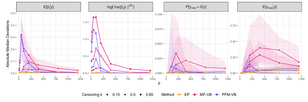
Figure 1: For four functionals of interest and different settings of $\kappa\in\{0.15,0.50,0.85\}$, trajectories for the median of the absolute differences, at varying $p$, between an accurate Monte Carlo estimate of such functionals via i.i.d. sampling from the exact SUN posterior and their approximation provided by mean-field variational Bayes (MF-VB), partially-factorized variational Bayes (PFM-VB) and expectation-propagation (EP) under tobit regression, with $n=200$. The shaded areas correspond to the first and third quartiles computed from the absolute differences. See the online article for the color version of this figure.

Table 1 illustrates the computational gains in sampling-based methods which can be obtained by leveraging routines that exploit directly the SUN conjugacy in Section 3. This is accomplished by comparing, for every combination of $\kappa$ and $p$, the runtimes to obtain $5000$ samples from the exact posterior distribution of ${\boldsymbol{\beta}}$ under both the routinely-used rstan implementation of the No-U-Turn HMC algorithm, and the i.i.d. sampler which exploits the additive representation of the SUN posterior in (11); refer to the code at https://github.com/niccoloanceschi/TobitSUN and to Chopin and Ridgway (2017) for details on the implementation of the HMC sampler in the class of models analyzed. The i.i.d. scheme leverages instead the R library TruncatedNormal (Botev, 2017) to sample the multivariate truncated normal component in (11). As discussed in Sections 4.1 and 4.2, such a task is inherently related, in terms of implementation and computational cost, to that of evaluating the Gaussian cumulative distribution functions required to conduct posterior inference under the closed-form expressions in Section 3.2. Nonetheless, Monte Carlo inference under i.i.d. samples has the additional benefit of allowing evaluation of any functional, even beyond those derived in closed form in Section 3.2, from a single set of samples, thereby motivating our focus on sampling-based methods which allow for a more comprehensive assessment.

Consistently with related findings on probit (Durante, 2019) and multinomial probit (Fasano and Durante, 2022), Table 1 confirms the computational gains of i.i.d. sampling relative to HMC in almost all the settings of $\kappa$ and $p$, especially when $p$ is large. In fact, while high-dimensional regimes are often challenging for HMC, under (11) $p$ only controls the dimension of the multivariate Gaussian, which is feasible to sample from, even for a large $p$. As discussed in Sections 4.1–4.2, more problematic for the i.i.d. scheme is the number of censored data $n_{0}$, which defines the dimension of the truncated normal in (11). This issue can be clearly seen in the increments of the runtimes under i.i.d.  sampling when the censoring percentage grows from $15\%$ to $85\%$. Nonetheless, the procedure is still competitive relative to HMC in these small-to-moderate $n_{0}$ settings. Notice also an increment in the runtime for the setting $\kappa=0.85$ (i.e., $n_{0}=170$), when $p\approx n_{0}/2$. In such a regime, the method by Botev (2017) experiences low acceptance probabilities with a trend over $n_{0}$ that is reminiscent of the double-descent phenomenon in high-dimensional regression (Hastie et al., 2022). This deserves further investigations.

As clarified in Table 1, the moderate dimensions of the simulated datasets would still allow posterior inference under the closed-form solutions and i.i.d. sampling schemes presented in Sections 4.1 and 4.2. Nonetheless, as previously discussed, when $n_{0}$ grows, these procedures become computationally impractical, thus motivating also the assessment of the more scalable approximate methods presented in Section 4.3. The relevant outcomes of these performance comparisons are reported in Figures 1–2 and in Table 2, with a focus on both accuracy and scalability. In particular, Figure 1 provides insights on the accuracy of MF-VB, PFM-VB and EP in approximating key posterior functionals of interest at varying $p$, and for the three different settings of $\kappa$. These quantities include the posterior mean and variance of each $\beta_{j}$ for $j=1,\ldots,p$, along with predictive measures for the expected value of the response $\mathbb{E}[\phi({\bf x}^{\intercal}_{\textsc{new},i}{\boldsymbol{\beta}})+({\bf x}^{\intercal}_{\textsc{new},i}{\boldsymbol{\beta}})\Phi({\bf x}^{\intercal}_{\textsc{new},i}{\boldsymbol{\beta}})\mid{\bf y}]$ and the probability of the censoring event $\mathbb{E}[\Phi(-{\bf x}^{\intercal}_{\textsc{new},i}{\boldsymbol{\beta}})\mid{\bf y}]$, both computed for $200$ test observations whose predictors are simulated as for the original training data. For such functionals, Figure 1 displays the medians and quartiles of the absolute differences between the corresponding Monte Carlo estimates under i.i.d. sampling from the exact SUN posterior and the approximations provided by the three methods analyzed, for varying $\kappa$ and $p$. In the first two panels, the three quartiles are computed on the $p$ absolute differences associated with coefficients $\beta_{1},\ldots,\beta_{p}$, whereas in the last two panels these summaries are calculated on the $200$ absolute differences for the $200$ test units. For what concerns the initialization of the variational routines, we consider the default setting which sets to zero the elements of the vectors $\mathbbm{E}_{q({\boldsymbol{\beta}},\bar{{\bf z}}_{-c})}({\boldsymbol{\mu}}_{c})$ and $\mathbbm{E}_{q(\bar{{\bf z}}_{-c})}(\bar{{\boldsymbol{\mu}}}_{c})$ in Equations (18) and (19), respectively, for all $c=1,\dots,C$. Analogously, in the case of EP we initialize the starting global approximation to the Gaussian density $l_{0}({\boldsymbol{\beta}})=p({\boldsymbol{\beta}}\mid\bar{{\bf y}}_{1})$, which corresponds to setting to zero the elements of the vectors ${\bf r}_{c}$ and matrices ${\bf Q}_{c}$ in Equation (23), for all $c=1,\dots,C$. In the absence of additional information, these initializations provide a sensible choice, which proved effective in a large number of experiments.

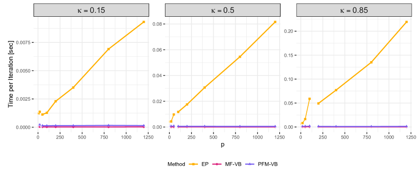
Figure 2: Runtimes, in seconds, for each iteration of mean-field variational Bayes (MF-VB), partially-factorized variational Bayes (PFM-VB) and expectation-propagation (EP) in tobit regression, for $n=200$ and different values of $p$ and $\kappa$. The runtimes are obtained as the median over 20 repetitions. The line breaks separate the result for two alternative implementations of each routine, optimizing the computational cost in $p$ and $n_{0}$. For the two variational procedures, the cost per iteration is $\mathcal{O}(n_{0}\cdot\min\{n_{0},p\})$, while for EP it becomes $\mathcal{O}(n_{0}p\cdot\min\{n_{0},p\})$. See the online article for the color version of this figure.

Table 2: Total runtimes in seconds (pre-computations, total iterations and post-computations), and number of iterations (within square brackets) required to reach convergence for mean-field variational Bayes (MF-VB), partially-factorized variational Bayes (PFM-VB) and expectation-propagation (EP) under tobit regression, with $n=200$. The reported runtimes are the medians over 20 repetitions.

p Censoring Method $10$ $20$ $50$ $100$ $200$ $400$ $800$ $1200$ $\kappa=0.85$ MF-VB $0.016$ [307] $0.046$ [719] $0.070$ [712] $0.134$ [828] $0.104$ [630] $0.129$ [675] $0.170$ [610] $0.219$ [571] PFM-VB $0.091$ [85] $0.237$ [192] $0.236$ [155] $0.262$ [140] $0.061$ [47] $0.039$ [13] $0.062$ [8] $0.100$ [7] EP $0.014$ [4] $0.018$ [4] $0.068$ [6] $0.270$ [5] $0.175$ [4] $0.252$ [3] $0.327$ [2] $0.488$ [2] $\kappa=0.50$ MF-VB $0.002$ [50] $0.004$ [87] $0.007$ [97] $0.020$ [194] $0.034$ [303] $0.050$ [236] $0.111$ [230] $0.197$ [248] PFM-VB $0.009$ [14] $0.016$ [23] $0.017$ [21] $0.024$ [32] $0.021$ [15] $0.033$ [6] $0.086$ [4] $0.165$ [3] EP $0.008$ [4] $0.008$ [3] $0.024$ [4] $0.050$ [4] $0.090$ [5] $0.142$ [4] $0.295$ [4] $0.459$ [4] $\kappa=0.15$ MF-VB $0.001$ [14] $0.001$ [19] $0.001$ [25] $0.003$ [46] $0.019$ [130] $0.043$ [111] $0.126$ [22] $0.253$ [7] PFM-VB $0.001$ [5] $0.002$ [6] $0.002$ [7] $0.003$ [8] $0.018$ [7] $0.042$ [3] $0.126$ [3] $0.253$ [3] EP $0.002$ [3] $0.002$ [3] $0.003$ [3] $0.005$ [3] $0.023$ [4] $0.052$ [4] $0.149$ [4] $0.278$ [3]

Consistently with Chopin and Ridgway (2017) and despite the limited theory guarantees, EP emerges as the most accurate solution in Figure 1 since its discrepancy from the Monte Carlo estimates under i.i.d. sampling is negligible in all regimes, ranging from $p<n_{0}$ to $p\geq n_{0}$. Nonetheless, as highlighted in Figure 2, the per-iteration runtimes of EP are linear in $p$ for high dimensions, as opposed to the quadratic growth in previously-available implementations, whereas those of MF-VB and PFM-VB are essentially constant and much lower. The impact of such a scaling in the cost per iteration on the overall runtime is relatively moderate in the regimes we focus on, as illustrated in Table 2 which displays the overall runtimes required by each routine to perform not only the total iterations, but also pre- and post-computations. Nonetheless, the higher per-iteration cost of EP becomes clearly appreciable when $p$ exceeds a few hundreds, as seen in Figure 2 and Table 2. Therefore, from a computational perspective, the variational routines are more effective and scalable alternatives in high-dimensional settings. This is especially true for PFM-VB which, as expected from the theory in Fasano, Durante, and Zanella (2022), attains the same accuracy of EP when $p\gtrsim 2n_{0}$, but with a lower computational effort. On the contrary, MF-VB is not competitive with EP in terms of accuracy and does not yield remarkable improvements in runtimes relative to PFM-VB in high dimensions. Notice that, although PFM-VB and MF-VB have the same per-iteration cost, the former does not allow for a joint updating of the approximating densities for the local variables, thus requiring a for cycle in basic R implementations that yields an increment in the per-iteration runtimes under PFM-VB, due to software-related inefficiencies. This drawback can be seen from Table 2, especially in those $p<n_{0}$ regimes where PFM-VB requires a moderate number of iterations to reach convergence.

Table 2 also displays the number of iterations needed by the three deterministic approximation procedures to reach convergence. Following common practice (e.g., Blei, Kucukelbir, and McAuliffe, 2017), the convergence for the two variational methods is intended as observing a difference below a suitable threshold between the ELBO of two consecutive iterations; see Fasano, Durante, and Zanella (2022); Consonni and Marin (2007) and the code in the GitHub repository for an expression of the ELBO under PFM-VB and MF-VB. The results presented in Table 2 correspond to a threshold of $10^{-3}$ on the logarithm of the ELBO. Conversely, as discussed in Section 4.3.2, EP routines do not share the same monotonicity and convergence guarantees that characterize variational routines. Therefore, the convergence of EP is commonly assessed in terms of the maximum absolute difference over the set of low dimensional parameters, characterizing the approximate Gaussian sites, between consecutive iterations (Chopin and Ridgway, 2017), for which we employ the same threshold as above. Consistent with the theoretical results in Fasano, Durante, and Zanella (2022), Table 2 provides evidence on the fact that the number of iterations needed by PFM-VB to reach convergence of the ELBO decays to one as $p$ grows to infinity, while also displaying the phenomenon reminiscent of double-descent noticed in Table 1, thus motivating further research along this line. Interestingly, the empirical results in Table 2 also suggest that the number of iterations required by EP does not grow with $p$. These analyses point toward EP as a default strategy, while suggesting PFM-VB as a feasible accurate alternative in high dimensions.

6 Discussion and future research directions

This review article provides a novel unified methodological and computational framework for Bayesian inference within a wide class of routinely-used regression models under a similarly broad set of prior distributions, which include the Gaussian one. Such an important gap in the literature is covered by first expressing the likelihoods associated with probit, tobit, multinomial probit and their extensions as special cases of a single formulation, and then generalizing previous findings for specific models in e.g., Durante (2019); Fasano and Durante (2022); Fasano et al. (2021); Cao, Durante, and Genton (2022); Benavoli, Azzimonti, and Piga (2020, 2021) to prove SUN (Arellano-Valle and Azzalini, 2006) conjugacy for any representation that admits such a unified likelihood. This yields general versions of past and more recent computational methods, previously proposed only for some specific members of the general class and with a focus on Gaussian priors. These include data-augmentation Gibbs samplers, i.i.d. sampling schemes, VB approximations and scalable EP implementations.

Due to the relevance of the models considered, such a review is expected to catalyze increasing interest by applied, computational and methodological researchers, and will hopefully motivate further research advancements along the directions opened by the results in Sections 2–5. For instance, the closed-form expressions in Section 3.2 for inference under the exact SUN posterior provide additional motivations to stimulate ongoing research aimed at developing accurate and fast methods to evaluate cumulative distribution functions of high-dimensional Gaussian distributions. In fact, any advancement along this direction and in sampling from multivariate truncated normals can be directly applied to conduct posterior inference via the closed-form results in Section 3.2, for increasingly larger sample sizes $\bar{n}+\bar{n}_{0}$, beyond small-to-moderate settings. This would be also useful for estimation of possible unknown parameters in the covariance matrices $\bar{{\boldsymbol{\Sigma}}}_{1}$ and $\bar{{\boldsymbol{\Sigma}}}_{0}$, via numerical maximization of the marginal likelihood $p({\bf y})$ in (13). As clarified in Sections 2.1–2.4 such matrices are often parameterized by a one-dimensional or low-dimensional vector of parameters, and hence, can be effectively estimated via direct maximization of $p({\bf y})$ when its evaluation is computationally practical. The availability of a closed-form expression (13) for $p({\bf y})$ and of i.i.d. sampling schemes from $({\boldsymbol{\beta}}\mid{\bf y})$ as in (11) can be also useful to facilitate full Bayesian inference for $\bar{{\boldsymbol{\Sigma}}}_{1}$ and $\bar{{\boldsymbol{\Sigma}}}_{0}$ when the associated parameters are assigned a prior. For example, leveraging $p({\bf y})$ it is possible to derive collapsed Metropolis–Hastings schemes to sample from the posteriors of $\bar{{\boldsymbol{\Sigma}}}_{1}$ and $\bar{{\boldsymbol{\Sigma}}}_{0}$ after integrating out ${\boldsymbol{\beta}}$ analytically, thereby improving mixing of data-augmentation MCMC (Park and Van Dyk, 2009); see also Chan and Jeliazkov (2009) for effective MCMC methods to infer $\bar{{\boldsymbol{\Sigma}}}_{0}$ under identifiability constraints. These advancements are beyond the scope of this review, but provide a research direction that is worth further exploration. Finally, it is also interesting to include hyperpriors for the scale parameters of the Gaussian or, more generally, SUN prior, that yield to scale-mixture representations inducing shrinkage in high dimensions (Carvalho, Polson, and Scott, 2010). Since most of these constructions rely on conditionally Gaussian priors, the results in the present review may be useful to obtain improved theoretical and practical performance in state-of-the-art implementations of the models in Section 2 under sparse settings; see Onorati and Liseo (2022) for recent advancements along these lines, motivated by SUN conjugacy.

Although (1) already encompasses several models of interest, further generalizations of such a likelihood and of the conjugacy results in Section 3 can be considered. For instance, it is possible to extend (1) to any version of the models in Sections 2.1–2.4 that arise from censoring or rounding of the Gaussian latent utilities into a generic truncation region. As discussed in the Supplementary Materials, such a mechanism is directly related to the generative construction of the broader class of selection distributions (SLCT) in Arellano-Valle, Branco, and Genton (2006). Hence, following the same general reasoning, it seems natural to prove SLCT conjugacy for this broader family of likelihoods. For example, this has been done in Kowal (2022) and King and Kowal (2021) by extending the ideas in Durante (2019) and Fasano et al. (2021) to static and dynamic rounded-data situations. These generalizations can be considered to prove similar conjugacy results for any extension of (1) which incorporates truncation into a finite region. It would be also interesting to extend the recent conjugacy results under skew-elliptical link functions, such as skew-$t$ (Branco and Dey, 2001; Azzalini and Capitanio, 2003; Gupta, 2003), to the proposed general framework. In fact, the unified skew-elliptical distribution (Arellano-Valle and Genton, 2010) has a general density expression that shares the product form of the likelihood (1), with a probability density function multiplied by a cumulative distribution function computed in some appropriate linear transformation of the parameter. This class of distributions admits as particular cases both the SUN and the unified skew-$t$ distribution, and thus also the skew-$t$. Motivated by these results, Zhang et al. (2021a) proved that unified skew-elliptical distributions are conjugate to probit and multinomial probit with skew-elliptical link functions, thus suggesting that this result may hold for any regression model based on skew-elliptical utilities.

As proved in a recent article by Durante, Pozza, and Szabo (2023), suitable generalizations of skew-normal distributions also provide more accurate limiting laws and skew-modal approximations for generic posterior distributions — beyond those considered in this article — with an improved convergence rate relative to the one achieved by the classical Bernstein–von Mises theorem based on limiting Gaussians.

Finally, it shall be also emphasized that the class of models discussed in Section 2 arguably encompasses one of the broadest set of formulations that appear in econometrics (Greene, 2008) and social sciences (DeMaris, 2004). Nonetheless, routine applications of such models under a Bayesian perspective have lagged behind the growing interest in Bayesian statistics. This review not only clarifies that the posterior distributions induced by the likelihoods of these models belong to a known class of variables, but also that such conjugacy results hold for a broader set of priors and for various extensions of classical probit, tobit and multinomial probit that are of direct relevance in econometrics and social sciences. This will hopefully boost the routine-use of these Bayesian models in applied research and motivate the development of even more flexible versions which still belong to likelihood (1), including, for example, random effects and graphical models (e.g., Jones et al., 2005).

SUPPLEMENTARY MATERIALS

The Supplementary Materials contain (i) further examples of relevant regression models whose likelihood can be re-written as in Equation (1), (ii) proofs of Lemma 1 and Theorem 1, and (iii) a detailed discussion on the computational costs of the routines to derive the approximations in Section 4.3. Code can be found at https://github.com/niccoloanceschi/TobitSUN.

S1 Further extensions to skewed link functions, non-linear models and dynamic settings

Although the models discussed in Sections 2.1, 2.2 and 2.3 cover the most widely-implemented formulations in the literature, as highlighted in Sections S1.1–S1.4 several additional extensions of these representations to skewed, non-linear, dynamic and other contexts can be reframed within the likelihood in (1).

S1.1 Inclusion of skewed latent utilities

S1.1.1 Skewed extensions of linear regression and multivariate linear regression

It is possible to include skewness within the formulations in Section 2.1, while still remaining in the class of models whose likelihood can be expressed as in (1). Recalling Sahu, Dey, and Branco (2003) and Azzalini (2005), this can be done by assuming that $(y_{i}\mid{\boldsymbol{\beta}})\sim\textsc{sn}({\bf x}^{\intercal}_{i}{\boldsymbol{\beta}},\sigma^{2},\alpha)$, independently for each $i=1,\ldots,n$, where $\textsc{sn}({\bf x}^{\intercal}_{i}{\boldsymbol{\beta}},\sigma^{2},\alpha)$ denotes the skew-normal distribution (Azzalini, 1985) with location ${\bf x}^{\intercal}_{i}{\boldsymbol{\beta}}$, scale $\sigma^{2}$ and shape parameter $\alpha$. This choice implies that

$$\begin{split}p({\bf y}\mid{\boldsymbol{\beta}})&\propto\prod\nolimits_{i=1}^{n}\phi(y_{i}-{\bf x}^{\intercal}_{i}{\boldsymbol{\beta}};\sigma^{2})\Phi(\alpha(y_{i}-{\bf x}^{\intercal}_{i}{\boldsymbol{\beta}});\sigma^{2})\\ &\ \ =\phi_{n}({\bf y}-{\bf X}{\boldsymbol{\beta}};\sigma^{2}{\bf I}_{n})\Phi_{n}(\alpha{\bf y}-\alpha{\bf X}{\boldsymbol{\beta}};\sigma^{2}{\bf I}_{n}),\end{split}$$ (S.1)

which coincides again with (1), when $\bar{n}_{1}=\bar{n}_{0}=n$, $\bar{{\bf y}}_{1}={\bf y}$, $\bar{{\bf y}}_{0}=\alpha{\bf y}$, $\bar{{\bf X}}_{1}={\bf X}$, $\bar{{\bf X}}_{0}=-\alpha{\bf X}$ and $\bar{{\boldsymbol{\Sigma}}}_{1}=\bar{{\boldsymbol{\Sigma}}}_{0}=\sigma^{2}{\bf I}_{n}$. Inclusion of skewed responses from more elaborated distributions such as the multivariate skew-normal (Azzalini and Dalla Valle, 1996; Azzalini and Capitanio, 1999), the extended multivariate skew-normal (Arnold and Beaver, 2000; Arnold et al., 2002), the closed skew-normal family (González-Farias, Dominguez-Molina, and Gupta, 2004; Gupta, González-Farias, and Dominguez-Molina, 2004) and the SUN (Arellano-Valle and Azzalini, 2006), is also possible and yields again special cases of Equation (1); see, e.g., Canale, Pagui, and Scarpa (2016).

S1.1.2 Skewed extensions of probit, multivariate probit and multinomial probit

The inclusion of skewed link functions is possible also under probit, multivariate probit and multinomial probit models. This direction has been effectively explored by Chen, Dey, and Shao (1999) and Bazán, Bolfarine, and Branco (2010) with a main focus on basic probit models, and can be again reframed within the general formulation in (1). For example, in the context of univariate probit regression, skewness can be incorporated by replacing the Gaussian latent utilities with skew-normal ones; namely $(z_{i}\mid{\boldsymbol{\beta}})\sim\textsc{sn}({\bf x}^{\intercal}_{i}{\boldsymbol{\beta}},\sigma^{2},\alpha)$, independently for $i=1,\ldots,n$. As a consequence, the binary response data $y_{i}=\mathbbm{1}(z_{i}>0)$ are Bernoulli variables with probabilities $\mbox{pr}(y_{i}=1\mid{\boldsymbol{\beta}})=\mbox{pr}(z_{i}>0\mid{\boldsymbol{\beta}})\propto\Phi_{2}[({\bf x}^{\intercal}_{i}{\boldsymbol{\beta}},0)^{\intercal};\mbox{diag}(\sigma^{2},1)+\sigma\alpha(1+\alpha^{2})^{-1/2}({\bf 1}_{2}{\bf 1}^{\intercal}_{2}-{\bf I}_{2})]$, whose expression follows directly from the cumulative distribution function of the skew-normal; see e.g., González-Farias, Dominguez-Molina, and Gupta (2004); Arellano-Valle and Azzalini (2006); Azzalini and Bacchieri (2010); Azzalini and Capitanio (2013), and Arellano-Valle and Azzalini (2021). Leveraging the same results, it also follows that $\mbox{pr}(y_{i}=0\mid{\boldsymbol{\beta}})=\mbox{pr}(z_{i}<0\mid{\boldsymbol{\beta}})\propto\Phi_{2}[(-{\bf x}^{\intercal}_{i}{\boldsymbol{\beta}},0)^{\intercal};\mbox{diag}(\sigma^{2},1)-\sigma\alpha(1+\alpha^{2})^{-1/2}({\bf 1}_{2}{\bf 1}^{\intercal}_{2}-{\bf I}_{2})]$. Let ${\bf X}_{i}=[(2y_{i}-1){\bf x}_{i},{\bf 0}]^{\intercal}$ and ${\boldsymbol{\Sigma}}_{i}=\mbox{diag}(\sigma^{2},1)+(2y_{i}-1)\sigma\alpha(1+\alpha^{2})^{-1/2}({\bf 1}_{2}{\bf 1}^{\intercal}_{2}-{\bf I}_{2})={\boldsymbol{\Sigma}}+(2y_{i}-1){\boldsymbol{\Lambda}}$, the joint likelihood for the binary response data can be then expressed as follows

$$\begin{split}p({\bf y}\mid{\boldsymbol{\beta}})&\propto\prod\nolimits_{i=1}^{n}\Phi_{2}({\bf X}_{i}{\boldsymbol{\beta}};{\boldsymbol{\Sigma}}_{i})\\ &\ \ \ =\Phi_{2n}({\bf X}{\boldsymbol{\beta}};{\bf I}_{n}\otimes{\boldsymbol{\Sigma}}+\mbox{diag}(2{\bf y}-{\bf 1}_{n})\otimes{\boldsymbol{\Lambda}}),\end{split}$$ (S.2)

with ${\bf X}=({\bf X}^{\intercal}_{1},\ldots,{\bf X}^{\intercal}_{n})^{\intercal}$, ${\boldsymbol{\Sigma}}=\mbox{diag}(\sigma^{2},1)$, and ${\boldsymbol{\Lambda}}=\sigma\alpha(1+\alpha^{2})^{-1/2}({\bf 1}_{2}{\bf 1}^{\intercal}_{2}-{\bf I}_{2})$. As a consequence, Equation (S.2) is again a special case of (1), after setting $\bar{n}_{1}=0$, $\bar{n}_{0}=2n$, $\bar{{\bf y}}_{0}={\bf 0}$, $\bar{{\bf X}}_{0}={\bf X}$ and $\bar{{\boldsymbol{\Sigma}}}_{0}={\bf I}_{n}\otimes{\boldsymbol{\Sigma}}+\mbox{diag}(2{\bf y}-{\bf 1}_{n})\otimes{\boldsymbol{\Lambda}}$. Similar derivations can be considered to incorporate skewness within multivariate and multinomial probit via multivariate skew-normal (Azzalini and Dalla Valle, 1996), closed skew-normal (González-Farias, Dominguez-Molina, and Gupta, 2004; Gupta, González-Farias, and Dominguez-Molina, 2004) or unified skew-normal (Arellano-Valle and Azzalini, 2006) latent utilities. Some of these choices have not yet been explored to induce skewed link functions for multivariate and multinomial extensions of classical probit regression. Nonetheless, all these variables have cumulative distribution functions proportional to those of multivariate Gaussians, evaluated at a linear combination of ${\boldsymbol{\beta}}$, and, hence, induce likelihoods which can be again expressed as special cases of the general framework in (1).

S1.1.3 Skewed extensions of tobit regression

As for the models presented in Sections 2.1 and 2.2, also tobit regression admits extensions to skewed contexts. This generalization has been explored, for example, by Hutton and Stanghellini (2011) who replace the Gaussian assumption for each $(z_{i}\mid{\boldsymbol{\beta}})\sim\mbox{N}({\bf x}^{\intercal}_{i}{\boldsymbol{\beta}},\sigma^{2})$ with the skew-normal $(z_{i}\mid{\boldsymbol{\beta}})\sim\textsc{sn}({\bf x}^{\intercal}_{i}{\boldsymbol{\beta}},\sigma^{2},\alpha)$, independently for every unit $i=1,\ldots,n$. Recalling the derivations for the skewed extensions of the models in Sections 2.1–2.2, this assumption implies that the contribution to the likelihood for the $i$–th data point is proportional to $(\phi(y_{i}-{\bf x}^{\intercal}_{i}{\boldsymbol{\beta}};\sigma^{2})\Phi[\alpha(y_{i}-{\bf x}^{\intercal}_{i}{\boldsymbol{\beta}});\sigma^{2}])^{\mathbbm{1}(y_{i}>0)}(\Phi_{2}[(-{\bf x}^{\intercal}_{i}{\boldsymbol{\beta}},0)^{\intercal};\mbox{diag}(\sigma^{2},1)-\sigma\alpha(1+~{}\alpha^{2})^{-1/2}$ $({\bf 1}_{2}{\bf 1}^{\intercal}_{2}-{\bf I}_{2})])^{\mathbbm{1}(y_{i}=0)}$. Therefore, letting $\mbox{diag}(\sigma^{2},1)={\boldsymbol{\Sigma}}$ and $\sigma\alpha(1+\alpha^{2})^{-1/2}({\bf 1}_{2}{\bf 1}^{\intercal}_{2}-{\bf I}_{2})={\boldsymbol{\Lambda}}$, yields

$$\begin{split}p({\bf y}\mid{\boldsymbol{\beta}})&\propto\prod\nolimits_{i:y_{i}>0}\phi(y_{i}-{\bf x}^{\intercal}_{i}{\boldsymbol{\beta}};\sigma^{2})\Phi(\alpha(y_{i}-{\bf x}^{\intercal}_{i}{\boldsymbol{\beta}});\sigma^{2})\\ &\qquad\cdot\prod\nolimits_{i:y_{i}=0}\Phi_{2}[(-{\bf x}^{\intercal}_{i}{\boldsymbol{\beta}},0)^{\intercal};{\boldsymbol{\Sigma}}-{\boldsymbol{\Lambda}}]\\ &\quad=\phi_{n_{1}}({\bf y}_{1}{-}{\bf X}_{1}{\boldsymbol{\beta}};\sigma^{2}{\bf I}_{n_{1}})\\ &\qquad\ \cdot\Phi_{n_{1}+2n_{0}}(\alpha[{\bf y}_{1}^{\intercal},{\bf 0}^{\intercal}]^{\intercal}-(\alpha{\bf X}_{1}^{\intercal},{\bf X}^{\intercal}_{0})^{\intercal}{\boldsymbol{\beta}};{\boldsymbol{\Sigma}}_{0}),\end{split}$$ (S.3)

where $n_{1}$, $n_{0}$, ${\bf y}_{1}$ and ${\bf X}_{1}$ are defined as in (7), whereas ${\bf X}_{0}$ is a $2n_{0}\times p$ design matrix obtained by stacking $2\times p$ row blocks ${\bf X}_{i}=({\bf x}_{i},{\bf 0})^{\intercal}$ for those units with $y_{i}=0$, while ${\boldsymbol{\Sigma}}_{0}$ is a block-diagonal matrix with blocks ${\boldsymbol{\Sigma}}_{0[1,1]}=\sigma^{2}{\bf I}_{n_{1}}$, ${\boldsymbol{\Sigma}}_{0[2,2]}={\bf I}_{n_{0}}\otimes{\boldsymbol{\Sigma}}-{\bf I}_{n_{0}}\otimes{\boldsymbol{\Lambda}}$. Hence, to express (S.3) as a particular case of (1) it suffices to set $\bar{n}_{1}=n_{1}$, $\bar{n}_{0}=n_{1}+2n_{0}$, $\bar{{\bf y}}_{1}={\bf y}_{1}$, $\bar{{\bf y}}_{0}=\alpha[{\bf y}_{1}^{\intercal},{\bf 0}^{\intercal}]^{\intercal}$, $\bar{{\bf X}}_{1}={\bf X}_{1}$, $\bar{{\bf X}}_{0}=-(\alpha{\bf X}_{1}^{\intercal},{\bf X}^{\intercal}_{0})^{\intercal}$, $\bar{{\boldsymbol{\Sigma}}}_{1}=\sigma^{2}{\bf I}_{n_{1}}$ and $\bar{{\boldsymbol{\Sigma}}}_{0}={\boldsymbol{\Sigma}}_{0}$. Recalling discussions in Sections 2.1–2.2, these derivations can be directly applied to incorporate skewness in type II–V tobit models (Amemiya, 1984), also under more general distributions which extend the original skew-normal (e.g., Arellano-Valle and Azzalini, 2006).

S1.2 Inclusion of generic thresholds

All the results presented in Sections 2.1–2.3 hold, under minor changes, when replacing the commonly-used zero threshold with a generic one $z_{\textsc{t}}$, possibly varying between units. For instance, in probit regression this modification implies that $\mbox{pr}(y_{i}=1\mid{\boldsymbol{\beta}})=\Phi(-z_{\textsc{t}}+{\bf x}^{\intercal}_{i}{\boldsymbol{\beta}})$, thus providing the joint likelihood $\prod_{i=1}^{n}\Phi[(2y_{i}-1)(-z_{\textsc{t}}+{\bf x}_{i}^{\intercal}{\boldsymbol{\beta}})]=\Phi_{n}(-z_{\textsc{t}}(2{\bf y}-{\bf 1}_{n})+\mbox{diag}(2{\bf y}-{\bf 1}_{n}){\bf X}{\boldsymbol{\beta}};{\bf I}_{n})$, which coincides with expression (1) after letting $\bar{n}_{1}=0$, $\bar{n}_{0}=n$, $\bar{{\bf y}}_{0}=-z_{\textsc{t}}(2{\bf y}-{\bf 1}_{n})$, $\bar{{\bf X}}_{0}=\mbox{diag}(2{\bf y}-{\bf 1}_{n}){\bf X}$ and $\bar{{\boldsymbol{\Sigma}}}_{0}={\bf I}_{n}$. Similar derivations apply to multivariate probit, multinomial probit, tobit, and their skewed extensions.

By contrast, all models relying on truncations to a finite interval of the form $[z_{1\textsc{t}},z_{2\textsc{t}}]$ do not induce likelihoods that can be rewritten as in (1). Nonetheless, these versions are less frequent than those presented in Sections 2.1–2.3 and, as discussed in Section 6, the SUN conjugacy results presented for the general class of models whose likelihoods admit the form (1), are useful to motivate similar extensions for a generic truncation mechanism. In fact, as discussed in Arellano-Valle, Branco, and Genton (2006), the SUN family belongs itself to an even more general class of selection distributions (SLCT) whose construction rely on cumulative distribution functions evaluated at generic intervals. This result has been recently leveraged by Kowal (2022) and King and Kowal (2021) to extend the original SUN conjugacy properties presented by Durante (2019) and Fasano et al. (2021) for probit regression and its multivariate dynamic extensions, respectively, to rounded/categorical data where truncation is in finite intervals (e.g., Jeliazkov, Graves, and Kutzbach, 2008). These modifications can be extended to prove the SLCT conjugacy for generalizations of (1) which admit truncation to any finite interval.

S1.3 Inclusion of non-linear effects

Another key extension of the models presented in Sections 2.1–2.3 can be obtained by including non-linearities within the predictor. A common solution to accomplish such a goal is to replace $f({\bf x}_{i})={\bf x}_{i}^{\intercal}{\boldsymbol{\beta}}$ with the generic basis expansion $f({\bf x}_{i})={\bf g}({\bf x}_{i})^{\intercal}{\boldsymbol{\beta}}$, where ${\bf g}({\bf x}_{i})=[g_{1}({\bf x}_{i}),\ldots,g_{k}({\bf x}_{i})]^{\intercal}$ are pre-specified non-linear basis functions, such as splines (see e.g., Holmes and Mallick, 2001; Lang and Brezger, 2004). Including this extension within the general framework in Equation (1) poses no difficulties since it is sufficient to replicate the derivations for the models presented in Sections 2.1, 2.2 and 2.3 with ${\bf x}_{i}=(x_{i1},\ldots,x_{ip})^{\intercal}$ replaced by $\tilde{{\bf x}}_{i}=[g_{1}({\bf x}_{i}),\ldots,g_{k}({\bf x}_{i})]^{\intercal}$, for each $i=1,\ldots,n$.

Alternatively, one can model directly $[f({\bf x}_{1}),\ldots,f({\bf x}_{n})]^{\intercal}\in\mathbbm{R}^{n}$ via a Gaussian process (e.g., Rasmussen and Williams, 2006). This direction has been commonly explored in the context of the models presented in Sections 2.1–2.3 (e.g., Kuss, Rasmussen, and Herbrich, 2005; De Oliveira, 2005; Girolami and Rogers, 2006; Nickisch and Rasmussen, 2008; Riihimäki, Jylänki, and Vehtari, 2014; Cao, Durante, and Genton, 2022; Benavoli, Azzimonti, and Piga, 2020, 2021), and can be also reframed within formulation (1). In particular, by assuming, without loss of generality, no overlap in ${\bf x}_{1},\ldots,{\bf x}_{n}$, the Gaussian process construction with mean function $m(\cdot)$ and covariance kernel $K(\cdot,\cdot)$ implies that $[f({\bf x}_{1}),\ldots,f({\bf x}_{n})]^{\intercal}$ is jointly distributed as a $\mbox{N}_{n}({\boldsymbol{\xi}},{\boldsymbol{\Omega}})$ with ${\boldsymbol{\xi}}=[m({\bf x}_{1}),\ldots,m({\bf x}_{n})]^{\intercal}$ and covariance matrix ${\boldsymbol{\Omega}}$ having entries ${\boldsymbol{\Omega}}_{ii^{\prime}}=K({\bf x}_{i},{\bf x}_{i^{\prime}})$, for each $i=1,\ldots,n$ and $i^{\prime}=1,\ldots,n$. This representation can be alternatively rewritten as $\tilde{{\bf X}}{\boldsymbol{\beta}}$, where ${\boldsymbol{\beta}}=[f({\bf x}_{1}),\ldots,f({\bf x}_{n})]^{\intercal}\sim\mbox{N}_{n}({\boldsymbol{\xi}},{\boldsymbol{\Omega}})$ and $\tilde{{\bf X}}={\bf I}_{n}$. Therefore, letting $\tilde{{\bf x}}_{i}$ denote an $n\times 1$ vector with value $1$ in position $i$ and $0$ elsewhere, for each $i=1,\ldots,n$, it is possible to consider Gaussian process extensions of the models in Sections 2.1–2.3, while still remaining within the general framework in (1).

S1.4 Inclusion of dynamic structure

Time–varying extensions of the models in Sections 2.1, 2.2 and 2.3 are common in the literature (e.g., Manrique and Shephard, 1998; Andrieu and Doucet, 2002; Naveau, Genton, and Shen, 2005; Chib and Jeliazkov, 2006; Soyer and Sung, 2013; Fasano et al., 2021). These extensions often appear as generalizations of the original dynamic linear model having observation equation $({\bf y}_{t}\mid{\boldsymbol{\beta}}_{t})\sim\mbox{N}_{m}({\bf X}_{t}{\boldsymbol{\beta}}_{t},{\boldsymbol{\Sigma}}_{t})$, independently for every time $t=1,\ldots,n$, and state equations $({\boldsymbol{\beta}}_{t}\mid{\boldsymbol{\beta}}_{t-1})\sim\mbox{N}_{p}({\bf G}_{t}{\boldsymbol{\beta}}_{t-1},{\bf W}_{t})$, independently for any $t=1,\ldots,n$, where ${\bf X}_{t}$, ${\boldsymbol{\Sigma}}_{t}$, ${\bf G}_{t}$, and ${\bf W}_{t}$ are known system matrices, whereas ${\boldsymbol{\beta}}_{0}\sim\mbox{N}_{p}({\bf a}_{0},{\bf P}_{0})$. This building-block construction implies that the contribution to the likelihood of ${\bf y}_{t}$, for every $t=1,\ldots,n$, is $p({\bf y}_{t}\mid{\boldsymbol{\beta}})=\phi_{m}({\bf y}_{t}-{\bf X}_{t}{\boldsymbol{\beta}}_{t};{\boldsymbol{\Sigma}}_{t})=\phi_{m}({\bf y}_{t}-\tilde{{\bf X}}_{t}{\boldsymbol{\beta}};{\boldsymbol{\Sigma}}_{t})$, where ${\boldsymbol{\beta}}=({\boldsymbol{\beta}}^{\intercal}_{1},\ldots,{\boldsymbol{\beta}}^{\intercal}_{n})^{\intercal}$ and $\tilde{{\bf X}}_{t}={\bf v}^{\intercal}_{t}\otimes{\bf X}_{t}$, with ${\bf v}_{t}$ denoting a $n\times 1$ indicator vector having value $1$ in position $t$ and $0$ elsewhere. Therefore, this representation can be directly interpreted as a particular version of the multivariate linear regression model in Equation (3) with covariance matrix possibly changing across the time units. Such a connection allows to directly recast the joint likelihood $p({\bf y}\mid{\boldsymbol{\beta}})$ of ${\bf y}=({\bf y}^{\intercal}_{1},\ldots,{\bf y}^{\intercal}_{n})^{\intercal}$ within (1). Clearly, this result holds for any subsequence ${\bf y}^{\intercal}_{1:t}=({\bf y}^{\intercal}_{1},\ldots,{\bf y}^{\intercal}_{t})^{\intercal}$, with $t=1,\ldots,n$, thereby facilitating online derivation of the filtering $p({\boldsymbol{\beta}}_{t}\mid{\bf y}_{1:t})$, predictive $p({\boldsymbol{\beta}}_{t+1}\mid{\bf y}_{1:t})$ and smoothing $p({\boldsymbol{\beta}}\mid{\bf y})$ distributions via the Gaussian-Gaussian conjugacy implied by the observation and state equations (Kalman, 1960).

The above results have been recently extended by Fasano et al. (2021) for deriving the first analog of the classical Kalman filter (Kalman, 1960) within the context of multivariate dynamic probit models with Gaussian states, leveraging the SUN–probit conjugacy properties proved in Durante (2019). Recalling Fasano et al. (2021) and adapting the notation to the one in this article, the contribution to the likelihood of ${\bf y}_{t}$, for every time $t=1,\ldots,n$, can be expressed as $p({\bf y}_{t}\mid{\boldsymbol{\beta}})=\Phi_{m}({\bf B}_{t}{\bf X}_{t}{\boldsymbol{\beta}}_{t};{\bf B}_{t}{\boldsymbol{\Sigma}}_{t}{\bf B}_{t})$, where ${\bf X}_{t}$ and ${\bf B}_{t}$ are defined as in (5), with $i$ replaced by time $t$, whereas ${\boldsymbol{\Sigma}}_{t}$ is a possibly time-varying covariance matrix among the latent utilities $(z_{t1},\ldots,z_{tm})^{\intercal}$. Recalling the derivations considered for the Gaussian dynamic setting, the expression for $p({\bf y}_{t}\mid{\boldsymbol{\beta}})$ can be alternatively rewritten as $p({\bf y}_{t}\mid{\boldsymbol{\beta}})=\Phi_{m}(\tilde{{\bf X}}_{t}{\boldsymbol{\beta}};{\bf B}_{t}{\boldsymbol{\Sigma}}_{t}{\bf B}_{t})$, with $\tilde{{\bf X}}_{t}={\bf v}^{\intercal}_{t}\otimes({\bf B}_{t}{\bf X}_{t})$, which shows again the direct connection between this dynamic formulation and its static counterpart in (5), thereby allowing to recast the induced joint likelihood for ${\bf y}=({\bf y}^{\intercal}_{1},\ldots,{\bf y}^{\intercal}_{n})^{\intercal}$ and its subsequences ${\bf y}^{\intercal}_{1:t}=({\bf y}^{\intercal}_{1},\ldots,{\bf y}^{\intercal}_{t})^{\intercal}$, $t=1,\ldots,n$, within Equation (1).

These results clearly hold also for the dynamic extensions of models (2) and (4), which represent the univariate versions of (3) and (5), respectively, thus simply requiring to set $m=1$ in the above derivations. Similarly, multinomial probit (6) and tobit (7) observation equations, along with skewed extensions ((S.1), (S.2), (S.3)), can be again reframed within (1) since all these constructions are characterized by contributions to the likelihood for each time $t=1,\ldots,n$ having the same form of those associated with the statistical units $i=1,\ldots,n$ in the static counterparts of such models presented in Sections 2.1–2.3, under suitable specifications of the design and covariance matrices.

As a final remark, it is worth emphasizing that (1) naturally encompasses any combination of the models discussed in Sections 2.1–2.4. For example, if ${\bf y}_{i}=(y_{i1},y_{i2},y_{i3},y_{i4})^{\intercal}$, where $y_{i1}$, $y_{i2}$, $y_{i3}$ and $y_{i4}$ are from models in (2), (4), (6) and (7), respectively, for each $i=1,\ldots,n$, then, leveraging the derivations in Sections 2.1–2.3, it directly follows that the joint likelihood for the vector ${\bf y}=({\bf y}^{\intercal}_{1},\ldots,{\bf y}^{\intercal}_{n})^{\intercal}$ still belongs to (1).

S2 Proofs of Lemma 1 and Theorem 1

Proof of Lemma 1.

To prove Lemma 1, first notice that, by Bayes rule

$$p({\boldsymbol{\beta}}\mid\bar{{\bf y}}_{1})\propto p({\boldsymbol{\beta}})p(\bar{{\bf y}}_{1}\mid{\boldsymbol{\beta}}),$$

where $p(\bar{{\bf y}}_{1}\mid{\boldsymbol{\beta}})=\phi_{\bar{n}_{1}}(\bar{{\bf y}}_{1}-\bar{{\bf X}}_{1}{\boldsymbol{\beta}};\bar{{\boldsymbol{\Sigma}}}_{1})$, whereas $p({\boldsymbol{\beta}})$ is the SUN density in (8). Leveraging Gaussian-Gaussian conjugacy, it follows that the product between $\phi_{\bar{n}_{1}}(\bar{{\bf y}}_{1}-\bar{{\bf X}}_{1}{\boldsymbol{\beta}};\bar{{\boldsymbol{\Sigma}}}_{1})$ and the density term $\phi_{\bar{p}}({\boldsymbol{\beta}}-{\boldsymbol{\xi}};{\boldsymbol{\Omega}})$ in (8) is proportional to $\phi_{\bar{p}}[{\boldsymbol{\beta}}-({\boldsymbol{\Omega}}^{-1}+\bar{{\bf X}}^{\intercal}_{1}\bar{{\boldsymbol{\Sigma}}}{}^{-1}_{1}\bar{{\bf X}}_{1})^{-1}({\boldsymbol{\Omega}}^{-1}{\boldsymbol{\xi}}+\bar{{\bf X}}^{\intercal}_{1}\bar{{\boldsymbol{\Sigma}}}{}^{-1}_{1}\bar{{\bf y}}_{1});({\boldsymbol{\Omega}}^{-1}+\bar{{\bf X}}^{\intercal}_{1}\bar{{\boldsymbol{\Sigma}}}{}^{-1}_{1}\bar{{\bf X}}_{1})^{-1}]=\phi_{\bar{p}}({\boldsymbol{\beta}}-{\boldsymbol{\xi}}_{1};{\boldsymbol{\Omega}}_{1})$, where

$$\begin{split}{\boldsymbol{\xi}}_{1}&=({\boldsymbol{\Omega}}^{-1}+\bar{{\bf X}}^{\intercal}_{1}\bar{{\boldsymbol{\Sigma}}}{}^{-1}_{1}\bar{{\bf X}}_{1})^{-1}({\boldsymbol{\Omega}}^{-1}{\boldsymbol{\xi}}+\bar{{\bf X}}^{\intercal}_{1}\bar{{\boldsymbol{\Sigma}}}{}^{-1}_{1}\bar{{\bf y}}_{1}),\\ {\boldsymbol{\Omega}}_{1}&=({\boldsymbol{\Omega}}^{-1}+\bar{{\bf X}}^{\intercal}_{1}\bar{{\boldsymbol{\Sigma}}}{}^{-1}_{1}\bar{{\bf X}}_{1})^{-1}={\boldsymbol{\omega}}_{1}\bar{{\boldsymbol{\Omega}}}_{1}{\boldsymbol{\omega}}_{1},\end{split}$$

Therefore, $p({\boldsymbol{\beta}}\mid\bar{{\bf y}}_{1})$ is proportional to the product between this updated Gaussian density and the cumulative distribution function term $\Phi_{\bar{n}}({\boldsymbol{\gamma}}+{\boldsymbol{\Delta}}^{\intercal}\bar{{\boldsymbol{\Omega}}}{}^{-1}{\boldsymbol{\omega}}^{-1}({\boldsymbol{\beta}}-{\boldsymbol{\xi}});{\boldsymbol{\Gamma}}-{\boldsymbol{\Delta}}^{\intercal}\bar{{\boldsymbol{\Omega}}}{}^{-1}{\boldsymbol{\Delta}})$ of the SUN density in (8), which can be also re-expressed as $\Phi_{\bar{n}}[{\bf s}^{-1}_{1}{\boldsymbol{\gamma}}+{\bf s}^{-1}_{1}{\boldsymbol{\Delta}}^{\intercal}\bar{{\boldsymbol{\Omega}}}{}^{-1}{\boldsymbol{\omega}}^{-1}({\boldsymbol{\beta}}-{\boldsymbol{\xi}});{\bf s}^{-1}_{1}({\boldsymbol{\Gamma}}-{\boldsymbol{\Delta}}^{\intercal}\bar{{\boldsymbol{\Omega}}}{}^{-1}{\boldsymbol{\Delta}}){\bf s}^{-1}_{1}]$, where ${\bf s}^{-1}_{1}$ is defined as in Lemma 1. To prove that this product yields to the SUN kernel in Lemma 1, rewrite ${\bf s}^{-1}_{1}{\boldsymbol{\gamma}}+{\bf s}^{-1}_{1}{\boldsymbol{\Delta}}^{\intercal}\bar{{\boldsymbol{\Omega}}}{}^{-1}{\boldsymbol{\omega}}^{-1}({\boldsymbol{\beta}}-{\boldsymbol{\xi}})$ as ${\bf s}^{-1}_{1}{\boldsymbol{\gamma}}-{\bf s}^{-1}_{1}{\boldsymbol{\Delta}}^{\intercal}\bar{{\boldsymbol{\Omega}}}{}^{-1}{\boldsymbol{\omega}}^{-1}{\boldsymbol{\xi}}+{\bf s}^{-1}_{1}{\boldsymbol{\Delta}}^{\intercal}\bar{{\boldsymbol{\Omega}}}{}^{-1}{\boldsymbol{\omega}}^{-1}{\boldsymbol{\beta}}$, and then sum and subtract ${\bf s}^{-1}_{1}{\boldsymbol{\Delta}}^{\intercal}\bar{{\boldsymbol{\Omega}}}{}^{-1}{\boldsymbol{\omega}}^{-1}{\boldsymbol{\xi}}_{1}$ inside this expression to obtain

$$\begin{split}&{\bf s}^{-1}_{1}[{\boldsymbol{\gamma}}+{\boldsymbol{\Delta}}^{\intercal}\bar{{\boldsymbol{\Omega}}}{}^{-1}{\boldsymbol{\omega}}^{-1}({\boldsymbol{\xi}}_{1}-{\boldsymbol{\xi}})]+{\bf s}^{-1}_{1}{\boldsymbol{\Delta}}^{\intercal}\bar{{\boldsymbol{\Omega}}}{}^{-1}{\boldsymbol{\omega}}^{-1}({\boldsymbol{\beta}}-{\boldsymbol{\xi}}_{1})\\ &={\boldsymbol{\gamma}}_{1}+{\bf s}^{-1}_{1}{\boldsymbol{\Delta}}^{\intercal}\bar{{\boldsymbol{\Omega}}}{}^{-1}{\boldsymbol{\omega}}^{-1}({\boldsymbol{\beta}}-{\boldsymbol{\xi}}_{1})\\ &={\boldsymbol{\gamma}}_{1}+{\bf s}^{-1}_{1}{\boldsymbol{\Delta}}^{\intercal}\bar{{\boldsymbol{\Omega}}}{}^{-1}{\boldsymbol{\omega}}^{-1}{\boldsymbol{\omega}}_{1}\bar{{\boldsymbol{\Omega}}}_{1}\bar{{\boldsymbol{\Omega}}}{}^{-1}_{1}{\boldsymbol{\omega}}{}^{-1}_{1}({\boldsymbol{\beta}}-{\boldsymbol{\xi}}_{1})\\ &={\boldsymbol{\gamma}}_{1}+{\boldsymbol{\Delta}}_{1}^{\intercal}\bar{{\boldsymbol{\Omega}}}_{1}{}^{-1}{\boldsymbol{\omega}}_{1}^{-1}({\boldsymbol{\beta}}-{\boldsymbol{\xi}}_{1}),\end{split}$$

with ${\boldsymbol{\gamma}}_{1}$ and ${\boldsymbol{\Delta}}_{1}$ defined as ${\boldsymbol{\gamma}}_{1}={\bf s}^{-1}_{1}[{\boldsymbol{\gamma}}+{\boldsymbol{\Delta}}^{\intercal}\bar{{\boldsymbol{\Omega}}}{}^{-1}{\boldsymbol{\omega}}^{-1}({\boldsymbol{\xi}}_{1}-{\boldsymbol{\xi}})]$ and ${\boldsymbol{\Delta}}_{1}=\bar{{\boldsymbol{\Omega}}}_{1}{\boldsymbol{\omega}}_{1}{\boldsymbol{\omega}}^{-1}\bar{{\boldsymbol{\Omega}}}{}^{-1}{\boldsymbol{\Delta}}{\bf s}^{-1}_{1}$, respectively. In order to conclude the proof, note that the correlation matrix within the cumulative distribution function term can be also rewritten as

$$\begin{split}&{\bf s}^{-1}_{1}({\boldsymbol{\Gamma}}-{\boldsymbol{\Delta}}^{\intercal}\bar{{\boldsymbol{\Omega}}}{}^{-1}{\boldsymbol{\Delta}}){\bf s}^{-1}_{1}\\ &={\bf s}^{-1}_{1}({\boldsymbol{\Gamma}}-{\boldsymbol{\Delta}}^{\intercal}\bar{{\boldsymbol{\Omega}}}{}^{-1}{\boldsymbol{\Delta}}){\bf s}^{-1}_{1}+{\boldsymbol{\Delta}}_{1}^{\intercal}\bar{{\boldsymbol{\Omega}}}{}^{-1}_{1}{\boldsymbol{\Delta}}_{1}-{\boldsymbol{\Delta}}_{1}^{\intercal}\bar{{\boldsymbol{\Omega}}}{}^{-1}_{1}{\boldsymbol{\Delta}}_{1}\\ &={\bf s}^{-1}_{1}[{\boldsymbol{\Gamma}}+{\boldsymbol{\Delta}}^{\intercal}(\bar{{\boldsymbol{\Omega}}}{}^{-1}{\boldsymbol{\omega}}^{-1}{\boldsymbol{\Omega}}_{1}{\boldsymbol{\omega}}^{-1}\bar{{\boldsymbol{\Omega}}}{}^{-1}-\bar{{\boldsymbol{\Omega}}}{}^{-1}){\boldsymbol{\Delta}}]{\bf s}^{-1}_{1}\\ &\qquad\qquad\qquad\qquad\qquad\qquad\qquad\qquad\qquad\quad-{\boldsymbol{\Delta}}_{1}^{\intercal}\bar{{\boldsymbol{\Omega}}}{}^{-1}_{1}{\boldsymbol{\Delta}}_{1},\end{split}$$

which corresponds to ${\boldsymbol{\Gamma}}_{1}-{\boldsymbol{\Delta}}_{1}^{\intercal}\bar{{\boldsymbol{\Omega}}}{}^{-1}_{1}{\boldsymbol{\Delta}}_{1}$, with ${\boldsymbol{\Gamma}}_{1}$ defined as in Lemma 1. This proves that the kernel $p({\boldsymbol{\beta}})p(\bar{{\bf y}}_{1}\mid{\boldsymbol{\beta}})$ of the posterior coincides with that of a SUN having parameters ${\boldsymbol{\xi}}_{1}$, ${\boldsymbol{\Omega}}_{1}$, ${\boldsymbol{\Delta}}_{1}$, ${\boldsymbol{\gamma}}_{1}$ and ${\boldsymbol{\Gamma}}_{1}$ specified as in Lemma 1. ∎

Proof of Theorem 1.

The proof of Theorem 1 simply requires to combine Lemma 1 with an adaptation of Corollary 4 in Durante (2019). In particular, by direct application of the Bayes rule, it follows that

$$p({\boldsymbol{\beta}}\mid{{\bf y}})\propto p({\boldsymbol{\beta}})p({\bf y}\mid{\boldsymbol{\beta}})\propto[p({\boldsymbol{\beta}})p(\bar{{\bf y}}_{1}\mid{\boldsymbol{\beta}})]p(\bar{{\bf y}}_{0}\mid{\boldsymbol{\beta}}).$$

Therefore, the posterior distribution $p({\boldsymbol{\beta}}\mid{{\bf y}})$ can be obtained by first updating the SUN prior $p({\boldsymbol{\beta}})$ with $p(\bar{{\bf y}}_{1}\mid{\boldsymbol{\beta}})\propto\phi_{\bar{n}_{1}}(\bar{{\bf y}}_{1}-\bar{{\bf X}}_{1}{\boldsymbol{\beta}};\bar{{\boldsymbol{\Sigma}}}_{1})$, and then use such a conditional density $p({\boldsymbol{\beta}}\mid\bar{{\bf y}}_{1})$ as an intermediate prior to be updated with the likelihood $p(\bar{{\bf y}}_{0}\mid{\boldsymbol{\beta}})\propto\Phi_{\bar{n}_{0}}(\bar{{\bf y}}_{0}+\bar{{\bf X}}_{0}{\boldsymbol{\beta}};\bar{{\boldsymbol{\Sigma}}}_{0})$ of $\bar{{\bf y}}_{0}$ for obtaining the final posterior. By direct application of Lemma 1, it follows that $p({\boldsymbol{\beta}}\mid\bar{{\bf y}}_{1})$ is the density of the $\mbox{SUN}_{\bar{p},\bar{n}}({\boldsymbol{\xi}}_{1},{\boldsymbol{\Omega}}_{1},{\boldsymbol{\Delta}}_{1},{\boldsymbol{\gamma}}_{1},{\boldsymbol{\Gamma}}_{1})$ with parameters defined as in Lemma 1. Therefore, to conclude the proof, it is sufficient to prove that the updating of this intermediate prior with the likelihood $p(\bar{{\bf y}}_{0}\mid{\boldsymbol{\beta}})\propto\Phi_{\bar{n}_{0}}(\bar{{\bf y}}_{0}+\bar{{\bf X}}_{0}{\boldsymbol{\beta}};\bar{{\boldsymbol{\Sigma}}}_{0})$ for $\bar{{\bf y}}_{0}$ yields again to a $\mbox{SUN}_{\bar{p},\bar{n}+\bar{n}_{0}}({\boldsymbol{\xi}}_{\mbox{\tiny post}},{\boldsymbol{\Omega}}_{\mbox{\tiny post}},{\boldsymbol{\Delta}}_{\mbox{\tiny post}},{\boldsymbol{\gamma}}_{\mbox{\tiny post}},{\boldsymbol{\Gamma}}_{\mbox{\tiny post}})$ with ${\boldsymbol{\xi}}_{\mbox{\tiny post}}$, ${\boldsymbol{\Omega}}_{\mbox{\tiny post}}$, ${\boldsymbol{\Delta}}_{\mbox{\tiny post}}$, ${\boldsymbol{\gamma}}_{\mbox{\tiny post}}$ and ${\boldsymbol{\Gamma}}_{\mbox{\tiny post}}$ defined as in Theorem 1. This result follows directly from an adaptation of Corollary 4 in Durante (2019); refer also to Theorem 1 in Fasano and Durante (2022). In particular, replacing ${\bf D}$ with $\bar{{\bf X}}_{0}$ and ${\bf I}_{n}$ with $\bar{{\boldsymbol{\Sigma}}}_{0}$ in Corollary 4 by Durante (2019), under a $\mbox{SUN}_{\bar{p},\bar{n}}({\boldsymbol{\xi}}_{1},{\boldsymbol{\Omega}}_{1},{\boldsymbol{\Delta}}_{1},{\boldsymbol{\gamma}}_{1},{\boldsymbol{\Gamma}}_{1})$ prior, yields to the expressions for ${\boldsymbol{\xi}}_{\mbox{\tiny post}}$, ${\boldsymbol{\Omega}}_{\mbox{\tiny post}}$, ${\boldsymbol{\Delta}}_{\mbox{\tiny post}}$ and ${\boldsymbol{\Gamma}}_{\mbox{\tiny post}}$ in Theorem 1. Inclusion of the offset $\bar{{\bf y}}_{0}$ in the proof of Corollary 4 by Durante (2019) poses no difficulties since it directly enters the SUN truncation parameter, thereby providing the expression for ${\boldsymbol{\gamma}}_{\mbox{\tiny post}}$ in Theorem 1. ∎

S3 Computational costs

To further extend the analysis of the approximate schemes in Sections 4.3.1–4.3.2, we discuss the associated cost per-iteration focusing, for the ease of notation, on the classical probit regression $\prod_{i=1}^{n}\Phi({\bf x}^{\intercal}_{i}{\boldsymbol{\beta}})^{\mathbbm{1}(y_{i}=1)}[1-\Phi({\bf x}^{\intercal}_{i}{\boldsymbol{\beta}})]^{\mathbbm{1}(y_{i}=0)}$ as in (4), with a spherical Gaussian prior $p({\boldsymbol{\beta}})=\phi_{p}({\boldsymbol{\beta}};\omega^{2}{\bf I}_{p})$. Note that, as discussed in Section 2.2, $n=\bar{n}_{0}$ and $p=\bar{p}$ when such a model is written as a special case of likelihood (1). Besides providing one of the most widely implemented formulations within the class of models whose likelihood can be expressed as in (1), this choice is also motivated by the fact that detailed costs per-iteration of effective MF-VB and PFM-VB implementations have been already derived in Fasano, Durante, and Zanella (2022) under probit regression with a Gaussian prior. Moreover, it gives the opportunity to show that currently-reported per-iteration costs of EP for the same class of models and priors (Chopin and Ridgway, 2017) can be further reduced, thus making also EP more scalable to high dimensions.

For deriving the costs of MF-VB, PFM-VB and EP it shall be emphasized that, in probit regression, such approximations rely on $c=1,\ldots,n$ and, therefore, $n_{c}=\bar{n}_{c}=1$ for any $c$. Under EP (Chopin and Ridgway, 2017) this choice is a common practice which follows from the factorized form of the likelihood, whereas in MF-VB (Consonni and Marin, 2007) it is implied by the formulation of the optimization problem and is a direct consequence of the conditional independence among the unit-specific latent utilities. Instead, for PFM-VB (Fasano, Durante, and Zanella, 2022) such a setting is not enforced. Nonetheless, it provides a convenient specification which is in line with MF-VB and EP solutions, and also facilitates posterior inference by only requiring to deal with univariate truncated normals.

Under the aforementioned settings, Appendix A of Fasano, Durante, and Zanella (2022) provides a detailed discussion of the per-iteration cost for both MF-VB and also PFM-VB, which is $\mathcal{O}(n\cdot\mbox{min}\{n,p\})=\mathcal{O}(\bar{n}_{0}\cdot\mbox{min}\{\bar{n}_{0},\bar{p}\})$, after suitable matrix precomputations before running the CAVI routine. Since the mean and variance of univariate truncated normals can be accurately computed at $\mathcal{O}(1)$ cost under standard algorithms (e.g., Botev, 2017), the most intensive computations in the CAVI routines for MF-VB and PFM-VB correspond to the matrix multiplication operations. These steps can be efficiently implemented by exploiting recursive formulas when updating each univariate truncated normal approximating density conditioned the most recent estimate of the others, in PFM-VB, or of the ${\boldsymbol{\beta}}$ parameters, in MF-VB, thereby leading to an overall per-iteration cost that is either linear or sublinear in $p=\bar{p}$.

As for EP, the currently reported per-iteration cost in probit regression with spherical Gaussian priors is $\mathcal{O}(np^{2})=\mathcal{O}(\bar{n}_{0}\bar{p}^{2})$ (Chopin and Ridgway, 2017), after suitable precomputations as in MF-VB and PFM-VB. Intuitively, this increased complexity is due to the fact that, unlike for MF-VB and PFM-VB, not only the expectations but also the $p\times p$ covariance matrices must be updated and then inverted at every site $c$, for each $c=1,\ldots,n$. Although the specific form of such matrices allows to reduce the common cubic cost into a quadratic one via the application of the Woodbury’s formula to avoid direct matrix inversion (Chopin and Ridgway, 2017), an $\mathcal{O}(np^{2})=\mathcal{O}(\bar{n}_{0}\bar{p}^{2})$ cost can be still computationally impractical in the large $p=\bar{p}$ setting. In fact, as mentioned in the final discussion by Chopin and Ridgway (2017), even the state-of-the-art implementations of EP are often computationally challenging when $p$ exceeds one thousand. This point is also confirmed in the empirical studies of Fasano, Durante, and Zanella (2022), where the EP implementation within the R package EPGLM by Chopin and Ridgway (2017) requires more than six hours to reach convergence in a high-dimensional Alzheimer’s application with $p=\bar{p}=9036$ and $n=\bar{n}_{0}=300$. Notably, as a further contribution of the present article, it shall be emphasized that a more scalable EP implementation with per-iteration cost $\mathcal{O}(np\cdot\mbox{min}\{n,p\})=\mathcal{O}(\bar{n}_{0}\bar{p}\cdot\mbox{min}\{\bar{n}_{0},\bar{p}\})$ can be actually derived by leveraging similar results considered in Fasano, Durante, and Zanella (2022) for obtaining efficient implementations of MF-VB and PFM-VB. In particular, this new EP implementation exploits the fact that, under the same reformulation via Woodbury’s identity of Chopin and Ridgway (2017), the site updates do not necessarily require direct computation of the aforementioned $p\times p$ matrices, since such quantities enter via the inner product with the $p\times n$ design matrices $\bar{{\bf X}}^{\intercal}_{0}$. Hence, when $p=\bar{p}$ is large, it is more convenient to update this product directly, without storing, updating or multiplying any $p\times p$ matrix. This yields to an $\mathcal{O}(np)=\mathcal{O}(\bar{n}_{0}\bar{p})$ cost for each site, and to an overall cost for the $n=\bar{n}_{0}$ site updates of $\mathcal{O}(n^{2}p)=\mathcal{O}(\bar{n}^{2}_{0}\bar{p})$. In high dimensional settings, when $p\gg n$, this linear cost in $p=\bar{p}$ yields to massive computational gains relative to the original $\mathcal{O}(np^{2})=\mathcal{O}(\bar{n}_{0}\bar{p}^{2})$ cost of EPGLM in Chopin and Ridgway (2017). For example, by considering the proposed more scalable implementation within the high-dimensional Alzheimer’s application yields to an overall runtime of less than one minute, which is orders of magnitude lower than EPGLM (Chopin and Ridgway, 2017) that requires, instead, more than six hours. When, instead, $n\gg p$, the linear cost in $n=\bar{n}_{0}$ of the EPGLM ensures effective implementations. Combining these two scenarios yields to an overall per-iteration cost of $\mathcal{O}(np\cdot\mbox{min}\{n,p\})=\mathcal{O}(\bar{n}_{0}\bar{p}\cdot\mbox{min}\{\bar{n}_{0},\bar{p}\})$, which is linear in the higher between $n=\bar{n}_{0}$ and $p=\bar{p}$. To the best of our knowledge, this is the first implementation of EP available in the literature to achieve such a computational efficiency. Despite this, standard EP remains more computationally demanding than MF-VB and PFM-VB since, as discussed above, also the $p\times p$ matrices need to be updated at each step of the EP routine, either directly or implicitly via the product with $\bar{{\bf X}}^{\intercal}_{0}$.

The above reasoning can be directly applied in order to highlight a similar dependence on sample size and number of predictors in the per-iteration cost of effective MF-VB, PFM-VB and EP implementations under the whole class of models and priors in Sections 2 and 3 — as long as $n_{c}$ and $\bar{n}_{c}$ are sufficiently small to allow the calculations of the moments for the associated multivariate truncated normals at a negligible cost compared to the one of the matrix operations. This result is illustrated in empirical studies in Section 5, with a focus on tobit regression.

References

- (1)
- Agresti (2013) Agresti, A. (2013), Categorical Data Analysis (Third Edition), Wiley.
- Albert and Chib (1993) Albert, J., and Chib, S. (1993), “Bayesian analysis of binary and polychotomous response data,” Journal of the American Statistical Association, 88, 669–679.
- Albert and Chib (2001) Albert, J.— (2001), “Sequential ordinal modeling with applications to survival data,” Biometrics, 57, 829–836.
- Amemiya (1984) Amemiya, T. (1984), “Tobit models: A survey,” Journal of Econometrics, 24, 3–61.
- Andrieu and Doucet (2002) Andrieu, C., and Doucet, A. (2002), “Particle filtering for partially observed Gaussian state space models,” Journal of the Royal Statistical Society: Series B, 64, 827–836.
- Arellano-Valle and Azzalini (2006) Arellano-Valle, R. B., and Azzalini, A. (2006), “On the unification of families of skew-normal distributions,” Scandinavian Journal of Statistics, 33, 561–574.
- Arellano-Valle and Azzalini (2021) Arellano-Valle, R. B.— (2021), “Some properties of the unified skew-normal distribution,” Statistical Papers, 63, 461–487.
- Arellano-Valle, Branco, and Genton (2006) Arellano-Valle, R. B., Branco, M. D., and Genton, M. G. (2006), “A unified view on skewed distributions arising from selections,” Canadian Journal of Statistics, 34, 581–601.
- Arellano-Valle and Genton (2010) Arellano-Valle, R. B., and Genton, M. G. (2010), “Multivariate unified skew-elliptical distributions,” Chilean Journal of Statistics, 1, 17–33.
- Arnold and Beaver (2000) Arnold, B. C., and Beaver, R. J. (2000), “Hidden truncation models,” Sankhyā: Series A, 62, 23–35.
- Arnold et al. (2002) Arnold, B. C., Beaver, R. J., Azzalini, A., Balakrishnan, N., Bhaumik, A., Dey, D., Cuadras, C., and Sarabia, J. M. (2002), “Skewed multivariate models related to hidden truncation and/or selective reporting,” Test, 11, 7–54.
- Azzalini (1985) Azzalini, A. (1985), “A class of distributions which includes the normal ones,” Scandinavian Journal of Statistics, 12, 171–178.
- Azzalini (2005) — (2005), “The skew-normal distribution and related multivariate families,” Scandinavian Journal of Statistics, 32, 159–188.
- Azzalini and Bacchieri (2010) Azzalini, A., and Bacchieri, A. (2010), “A prospective combination of phase II and phase III in drug development,” Metron, 68, 347–369.
- Azzalini and Capitanio (1999) Azzalini, A., and Capitanio, A. (1999), “Statistical applications of the multivariate skew normal distribution,” Journal of the Royal Statistical Society: Series B, 61, 579–602.
- Azzalini and Capitanio (2003) Azzalini, A.— (2003), “Distributions generated by perturbation of symmetry with emphasis on a multivariate skew t-distribution,” Journal of the Royal Statistical Society: Series B, 65, 367–389.
- Azzalini and Capitanio (2013) Azzalini, A.— (2013), The Skew-Normal and Related Families, Cambridge University Press.
- Azzalini and Dalla Valle (1996) Azzalini, A., and Dalla Valle, A. (1996), “The multivariate skew-normal distribution,” Biometrika, 83, 715–726.
- Bazán, Bolfarine, and Branco (2010) Bazán, J. L., Bolfarine, H., and Branco, M. D. (2010), “A framework for skew-probit links in binary regression,” Communications in Statistics–Theory and Methods, 39, 678–697.
- Benavoli, Azzimonti, and Piga (2020) Benavoli, A., Azzimonti, D., and Piga, D. (2020), “Skew Gaussian processes for classification,” Machine Learning, 109, 1877–1902.
- Benavoli, Azzimonti, and Piga (2021) Benavoli, A.— (2021), “A unified framework for closed–form nonparametric regression, classification, preference and mixed problems with skew Gaussian processes,” Machine Learning, 110, 3095–3133.
- Bishop (2006) Bishop, C. (2006), Pattern Recognition and Machine Learning, Springer.
- Blei, Kucukelbir, and McAuliffe (2017) Blei, D. M., Kucukelbir, A., and McAuliffe, J. D. (2017), “Variational inference: A review for statisticians,” Journal of the American Statistical Association, 112, 859–877.
- Bliss (1934) Bliss, C. I. (1934), “The method of probits,” Science, 79, 38–39.
- Botev (2017) Botev, Z. I. (2017), “The normal law under linear restrictions: Simulation and estimation via minimax tilting,” Journal of the Royal Statistical Society: Series B, 88, 125–148.
- Branco and Dey (2001) Branco, M. D., and Dey, D. K. (2001), “A general class of multivariate skew-elliptical distributions,” Journal of Multivariate Analysis, 79, 99–113.
- Canale, Pagui, and Scarpa (2016) Canale, A., Pagui, E. C. K., and Scarpa, B. (2016), “Bayesian modeling of university first-year students’ grades after placement test,” Journal of Applied Statistics, 43, 3015–3029.
- Cao, Durante, and Genton (2022) Cao, J., Durante, D., and Genton, M. G. (2022), “Scalable computation of predictive probabilities in probit models with Gaussian process priors,” Journal of Computational and Graphical Statistics, 31, 709–720.
- Cao et al. (2019) Cao, J., Genton, M. G., Keyes, D. E., and Turkiyyah, G. M. (2019), “Hierarchical-block conditioning approximations for high-dimensional multivariate normal probabilities,” Statistics and Computing, 29, 585–598.
- Cao et al. (2021) Cao, J.— (2021), “Exploiting low-rank covariance structures for computing high-dimensional normal and Student-t probabilities,” Statistics and Computing, 31, 1–16.
- Carvalho, Polson, and Scott (2010) Carvalho, C. M., Polson, N. G., and Scott, J. G. (2010), “The horseshoe estimator for sparse signals,” Biometrika, 97, 465–480.
- Chan and Jeliazkov (2009) Chan, J. C.-C., and Jeliazkov, I. (2009), “MCMC estimation of restricted covariance matrices,” Journal of Computational and Graphical Statistics, 18, 457–480.
- Chen, Dey, and Shao (1999) Chen, M.-H., Dey, D. K., and Shao, Q.-M. (1999), “A new skewed link model for dichotomous quantal response data,” Journal of the American Statistical Association, 94, 1172–1186.
- Chib (1992) Chib, S. (1992), “Bayes inference in the tobit censored regression model,” Journal of Econometrics, 51, 79 – 99.
- Chib and Greenberg (1998) Chib, S., and Greenberg, E. (1998), “Analysis of multivariate probit models,” Biometrika, 85, 347–361.
- Chib, Greenberg, and Jeliazkov (2009) Chib, S., Greenberg, E., and Jeliazkov, I. (2009), “Estimation of semiparametric models in the presence of endogeneity and sample selection,” Journal of Computational and Graphical Statistics, 18, 321–348.
- Chib and Jeliazkov (2006) Chib, S., and Jeliazkov, I. (2006), “Inference in semiparametric dynamic models for binary longitudinal data,” Journal of the American Statistical Association, 101, 685–700.
- Chipman, George, and McCulloch (2010) Chipman, H. A., George, E. I., and McCulloch, R. E. (2010), “BART: Bayesian additive regression trees,” The Annals of Applied Statistics, 4, 266–298.
- Chopin and Ridgway (2017) Chopin, N., and Ridgway, J. (2017), “Leave Pima Indians alone: Binary regression as a benchmark for Bayesian computation,” Statistical Science, 32, 64–87.
- Consonni and Marin (2007) Consonni, G., and Marin, J.-M. (2007), “Mean-field variational approximate Bayesian inference for latent variable models,” Computational Statistics & Data Analysis, 52, 790–798.
- Craig (2008) Craig, P. (2008), “A new reconstruction of multivariate normal orthant probabilities,” Journal of the Royal Statistical Society: Series B, 70, 227–243.
- De Oliveira (2005) De Oliveira, V. (2005), “Bayesian inference and prediction of Gaussian random fields based on censored data,” Journal of Computational and Graphical Statistics, 14, 95–115.
- Dehaene and Barthelmé (2018) Dehaene, G., and Barthelmé, S. (2018), “Expectation propagation in the large data limit,” Journal of the Royal Statistical Society: Series B, 80, 199–217.
- DeMaris (2004) DeMaris, A. (2004), Regression with Social Data: Modeling Continuous and Limited Response Variables, John Wiley & Sons.
- Durante (2019) Durante, D. (2019), “Conjugate Bayes for probit regression via unified skew-normal distributions,” Biometrika, 106, 765–779.
- Durante, Pozza, and Szabo (2023) Durante, D., Pozza, F., and Szabo, B. T. (2023), “Skewed Bernstein–von Mises theorem and skew-modal approximations,” arXiv:2301.03038.
- Fasano and Durante (2022) Fasano, A., and Durante, D. (2022), “A class of conjugate priors for multinomial probit models which includes the multivariate normal one,” Journal of Machine Learning Research, 23, 1–26.
- Fasano, Durante, and Zanella (2022) Fasano, A., Durante, D., and Zanella, G. (2022), “Scalable and accurate variational Bayes for high-dimensional binary regression models,” Biometrika, 109, 901–919.
- Fasano et al. (2021) Fasano, A., Rebaudo, G., Durante, D., and Petrone, S. (2021), “A closed-form filter for binary time series,” Statistics and Computing, 31, 1–20.
- Galarza Morales et al. (2022) Galarza Morales, C. E., Matos, L. A., Dey, D. K., and Lachos, V. H. (2022), “On moments of folded and doubly truncated multivariate extended skew-normal distributions,” Journal of Computational and Graphical Statistics, 31, 455–465.
- Gassmann (2003) Gassmann, H. (2003), “Multivariate normal probabilities: implementing an old idea of Plackett’s,” Journal of Computational and Graphical Statistics, 12, 731–752.
- Gelman, Jakulin, and Su (2008) Gelman, A., Jakulin, A., G., P. M., and Su, Y. (2008), “A weakly informative default prior distribution for logistic and other regression models,” The Annals of Applied Statistics, 2, 1360–1383.
- Genton, Keyes, and Turkiyyah (2018) Genton, M., Keyes, D., and Turkiyyah, G. (2018), “Hierarchical decompositions for the computation of high-dimensional multivariate normal probabilities,” Journal of Computational and Graphical Statistics, 27, 268–277.
- Genz (1992) Genz, A. (1992), “Numerical computation of multivariate normal probabilities,” Journal of Computational and Graphical Statistics, 1, 141–149.
- Genz (2004) — (2004), “Numerical computation of rectangular bivariate and trivariate normal and t probabilities,” Statistics and Computing, 14, 251–260.
- Genz and Bretz (2002) Genz, A., and Bretz, F. (2002), “Comparison of methods for the computation of multivariate t probabilities,” Journal of Computational and Graphical Statistics, 11, 950–971.
- Genz and Bretz (2009) Genz, A.— (2009), Computation of Multivariate Normal and t Probabilities, Springer.
- Gessner, Kanjilal, and Hennig (2020) Gessner, A., Kanjilal, O., and Hennig, P. (2020), “Integrals over Gaussians under linear domain constraints,” in Artificial Intelligence and Statistics, PMLR, pp. 2764–2774.
- Girolami and Rogers (2006) Girolami, M., and Rogers, S. (2006), “Variational Bayesian multinomial probit regression with Gaussian process priors,” Neural Computation, 18, 1790–1817.
- González-Farias, Dominguez-Molina, and Gupta (2004) González-Farias, G., Dominguez-Molina, A., and Gupta, A. K. (2004), “Additive properties of skew normal random vectors,” Journal of Statistical Planning and Inference, 126, 521–534.
- Greene (2008) Greene, W. (2008), Econometric Analysis, Pearson Education India.
- Gupta (2003) Gupta, A. (2003), “Multivariate skew t-distribution,” Statistics: A Journal of Theoretical and Applied Statistics, 37, 359–363.
- Gupta, González-Farias, and Dominguez-Molina (2004) Gupta, A. K., González-Farias, G., and Dominguez-Molina, J. A. (2004), “A multivariate skew normal distribution,” Journal of Multivariate Analysis, 89, 181–190.
- Hastie et al. (2022) Hastie, T., Montanari, A., Rosset, S., and Tibshirani, R. J. (2022), “Surprises in high-dimensional ridgeless least squares interpolation,” The Annals of Statistics, 50, 949–986.
- Hausman and Wise (1978) Hausman, J., and Wise, D. (1978), “A conditional probit model for qualitative choice: Discrete decisions recognizing interdependence and heterogeneous preferences,” Econometrica, 46, 403–426.
- Hoffman and Gelman (2014) Hoffman, M. D., and Gelman, A. (2014), “The No-U-Turn sampler: Adaptively setting path lengths in Hamiltonian Monte Carlo,” Journal of Machine Learning Research, 15, 1593–1623.
- Holmes and Held (2006) Holmes, C. C., and Held, L. (2006), “Bayesian auxiliary variable models for binary and multinomial regression,” Bayesian Analysis, 1, 145–168.
- Holmes and Mallick (2001) Holmes, C., and Mallick, B. (2001), “Bayesian regression with multivariate linear splines,” Journal of the Royal Statistical Society: Series B, 63, 3–17.
- Horrace (2005) Horrace, W. (2005), “Some results on the multivariate truncated normal distribution,” Journal of Multivariate Analysis, 94, 209–221.
- Hutton and Stanghellini (2011) Hutton, J., and Stanghellini, E. (2011), “Modelling bounded health scores with censored skew-normal distributions,” Statistics in Medicine, 30, 368–376.
- Imai and Van Dyk (2005) Imai, K., and Van Dyk, D. (2005), “A Bayesian analysis of the multinomial probit model using marginal data augmentation,” Journal of Econometrics, 124, 311–334.
- Jeliazkov, Graves, and Kutzbach (2008) Jeliazkov, I., Graves, J., and Kutzbach, M. (2008), “Fitting and comparison of models for multivariate ordinal outcomes,” in Bayesian Econometrics, vol. 23, pp. 115–156.
- Johndrow, Dunson, and Lum (2013) Johndrow, J., Dunson, D., and Lum, K. (2013), “Diagonal orthant multinomial probit models,” in Artificial Intelligence and Statistics, PMLR, pp. 29–38.
- Johndrow et al. (2018) Johndrow, J. E., Smith, A., Pillai, N., and Dunson, D. B. (2018), “MCMC for imbalanced categorical data,” Journal of the American Statistical Association, 114, 1394–1403.
- Jones et al. (2005) Jones, B., Carvalho, C., Dobra, A., Hans, C., Carter, C., and West, M. (2005), “Experiments in stochastic computation for high-dimensional graphical models,” Statistical Science, 20, 388–400.
- Kalman (1960) Kalman, R. E. (1960), “A new approach to linear filtering and prediction problems,” Journal of Basic Engineering, 82, 35–45.
- King and Kowal (2021) King, B., and Kowal, D. R. (2021), “Warped dynamic linear models for time series of counts,” arXiv:2110.14790.
- Kowal (2022) Kowal, D. R. (2022), “Semiparametric discrete data regression with Monte Carlo inference and prediction,” arXiv:2110.12316.
- Kullback and Leibler (1951) Kullback, S., and Leibler, R. (1951), “On information and sufficiency,” The Annals of Mathematical Statistics, 22, 79 – 86.
- Kuss, Rasmussen, and Herbrich (2005) Kuss, M., Rasmussen, C. E., and Herbrich, R. (2005), “Assessing approximate inference for binary Gaussian process classification,” Journal of Machine Learning Research, 6, 1679–1704.
- Lang and Brezger (2004) Lang, S., and Brezger, A. (2004), “Bayesian P-splines,” Journal of Computational and Graphical Statistics, 13, 183–212.
- Loaiza-Maya and Nibbering (2022) Loaiza-Maya, R., and Nibbering, D. (2022), “Scalable Bayesian estimation in the multinomial probit model,” Journal of Business & Economic Statistics, 40, 1678–1690.
- Loaiza-Maya et al. (2022) Loaiza-Maya, R., Smith, M. S., Nott, D. J., and Danaher, P. J. (2022), “Fast and accurate variational inference for models with many latent variables,” Journal of Econometrics, 230, 339–362.
- Manrique and Shephard (1998) Manrique, A., and Shephard, N. (1998), “Simulation-based likelihood inference for limited dependent processes,” The Econometrics Journal, 1, 174–202.
- McCulloch, Polson, and Rossi (2000) McCulloch, R., Polson, N., and Rossi, P. (2000), “A Bayesian analysis of the multinomial probit model with fully identified parameters,” Journal of Econometrics, 99, 173–193.
- McCulloch and Rossi (1994) McCulloch, R., and Rossi, P. (1994), “An exact likelihood analysis of the multinomial probit model,” Journal of Econometrics, 64, 207–240.
- Minka (2001) Minka, T. P. (2001), “Expectation propagation for approximate Bayesian inference,” Proceedings of Uncertainty in Artificial Intelligence, 17, 362–369.
- Miwa, Hayter, and Kuriki (2003) Miwa, T., Hayter, A., and Kuriki, S. (2003), “The evaluation of general non-centred orthant probabilities,” Journal of the Royal Statistical Society: Series B, 65, 223–234.
- Naveau, Genton, and Shen (2005) Naveau, P., Genton, M. G., and Shen, X. (2005), “A skewed Kalman filter,” Journal of Multivariate Analysis, 94, 382–400.
- Nickisch and Rasmussen (2008) Nickisch, H., and Rasmussen, C. E. (2008), “Approximations for binary Gaussian process classification,” Journal of Machine Learning Research, 9, 2035–2078.
- Nobile (1998) Nobile, A. (1998), “A hybrid Markov chain for the Bayesian analysis of the multinomial probit model,” Statistics and Computing, 8, 229–242.
- Onorati and Liseo (2022) Onorati, P., and Liseo, B. (2022), “An extension of the Unified Skew-Normal family of distributions and application to Bayesian binary regression,” arXiv:2209.03474.
- Pakman and Paninski (2014) Pakman, A., and Paninski, L. (2014), “Exact Hamiltonian Monte Carlo for truncated multivariate Gaussians,” Journal of Computational and Graphical Statistics, 23, 518–542.
- Park and Van Dyk (2009) Park, T., and Van Dyk, D. A. (2009), “Partially collapsed Gibbs samplers: Illustrations and applications,” Journal of Computational and Graphical Statistics, 18, 283–305.
- Qin and Hobert (2019) Qin, Q., and Hobert, J. P. (2019), “Convergence complexity analysis of Albert and Chib’s algorithm for Bayesian probit regression,” The Annals of Statistics, 47, 2320–2347.
- Rasmussen and Williams (2006) Rasmussen, C. E., and Williams, C. K. I. (2006), Gaussian Processes for Machine Learning, MIT Press.
- Ridgway (2016) Ridgway, J. (2016), “Computation of Gaussian orthant probabilities in high dimension,” Statistics and Computing, 26, 899–916.
- Riihimäki, Jylänki, and Vehtari (2014) Riihimäki, J., Jylänki, P., and Vehtari, A. (2014), “Nested expectation propagation for Gaussian process classification with a multinomial probit likelihood,” Journal of Machine Learning Research, 14, 75–109.
- Roberts and Rosenthal (2001) Roberts, G. O., and Rosenthal, J. S. (2001), “Optimal scaling for various Metropolis-Hastings algorithms,” Statistical Science, 16, 351–367.
- Rodriguez and Dunson (2011) Rodriguez, A., and Dunson, D. (2011), “Nonparametric Bayesian models through probit stick-breaking processes,” Bayesian Analysis, 6, 145–178.
- Rue, Martino, and Chopin (2009) Rue, H., Martino, S., and Chopin, N. (2009), “Approximate Bayesian inference for latent Gaussian models by using integrated nested Laplace approximations,” Journal of the Royal Statistical Society: Series B, 71, 319–392.
- Sahu, Dey, and Branco (2003) Sahu, S. K., Dey, D. K., and Branco, M. D. (2003), “A new class of multivariate skew distributions with applications to Bayesian regression models,” Canadian Journal of Statistics, 31, 129–150.
- Soyer and Sung (2013) Soyer, R., and Sung, M. (2013), “Bayesian dynamic probit models for the analysis of longitudinal data,” Computational Statistics & Data Analysis, 68, 388–398.
- Stern (1992) Stern, S. (1992), “A method for smoothing simulated moments of discrete probabilities in multinomial probit models,” Econometrica, 60, 943–952.
- Talhouk, Doucet, and Murphy (2012) Talhouk, A., Doucet, A., and Murphy, K. (2012), “Efficient Bayesian inference for multivariate probit models with sparse inverse correlation matrices,” Journal of Computational and Graphical Statistics, 21, 739–757.
- Tobin (1958) Tobin, J. (1958), “Estimation of relationships for limited dependent variables,” Econometrica, 26, 24–36.
- Trinh and Genz (2015) Trinh, G., and Genz, A. (2015), “Bivariate conditioning approximations for multivariate normal probabilities,” Statistics and Computing, 25, 989–996.
- Tutz (1991) Tutz, G. (1991), “Sequential models in categorical regression,” Computational Statistics & Data Analysis, 11, 275–295.
- Vehtari et al. (2020) Vehtari, A., Gelman, A., Sivula, T., Jylänki, P., Tran, D., Sahai, S., Blomstedt, P., Cunningham, J., Schiminovich, D., and Robert, C. (2020), “Expectation propagation as a way of life: A framework for Bayesian inference on partitioned data,” Journal of Machine Learning Research, 21, 1–53.
- Zellner (1986) Zellner, A. (1986), “On assessing prior distributions and Bayesian regression analysis with g–prior distributions,” Bayesian Inference and Decision Techniques: Essays in Honor of Bruno de Finetti, 233–243.
- Zhang et al. (2021a) Zhang, Z., Arellano-Valle, R. B., Genton, M. G., and Huser, R. (2021a), “Tractable Bayes of skew-elliptical link models for correlated binary data,” Biometrics, In press.
- Zhang et al. (2021b) Zhang, Z., Nishimura, A., Bastide, P., Ji, X., Payne, R. P., Goulder, P., Lemey, P., and Suchard, M. A. (2021b), “Large-scale inference of correlation among mixed-type biological traits with phylogenetic multivariate probit models,” The Annals of Applied Statistics, 15, 230–251.