Towards More Objective Evaluation of Class Incremental Learning
: Representation Learning Perspective

Abstract

Class incremental learning (CIL) is the process of continually learning new object classes from incremental data while not forgetting past learned classes. While the common method for evaluating CIL algorithms is based on average test accuracy for all learned classes, we argue that maximizing accuracy alone does not necessarily lead to effective CIL algorithms. In this paper, we experimentally analyze neural network models trained by CIL algorithms using various evaluation protocols in representation learning and propose a new analysis method. Our experiments show that most state-of-the-art algorithms prioritize high stability and do not significantly change the learned representation, and sometimes even learn a representation of lower quality than a naive baseline. However, we observe that these algorithms can still achieve high test accuracy because they learn a classifier that is closer to the optimal classifier. We also found that the base model learned in the first task varies in representation quality across different algorithms, and changes in the final performance were observed when each algorithm was trained under similar representation quality of the base model. Thus, we suggest that representation-level evaluation is an additional recipe for more objective evaluation and effective development of CIL algorithms.

1 Introduction

Neural networks have achieved great success in various fields such as computer vision, natural language processing, and reinforcement learning [26, 5]. Among these fields, image classification was the first representative task leading to the significant progress of neural networks [12, 25, 21]. Furthermore, the ImageNet pretrained model has been widely used as an initial model for transfer learning in other downstream tasks, such as object detection, semantic segmentation, and other classification datasets. In terms of representation learning, experimental analyses have shown that models achieving better classification accuracy learn better quality of representations, leading to better ability for transfer learning to various downstream tasks [24].

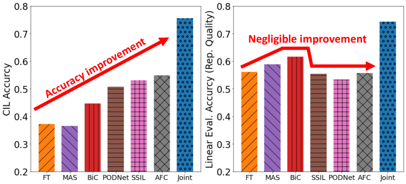
Figure 1: The accuracy of state-of-the-art CIL algorithms has been gradually increasing, approaching that of Joint training (left). However, we experimentally confirm that the improvement of the quality of representations learned by them is negligible or even worse than naive baselines (right).

However, neural networks exhibit a significant gap with humans in their ability to continually learn from a series of tasks. To narrow this gap, research on Continual Learning (CL) has started, beginning with image classification as the representative task [34, 11, 31]. Among the three scenarios of CL, Class Incremental Learning (CIL) is considered an important sub-category that has drawn a lot of attention [40, 31]. This setting models a practical scenario that can be encountered in many real-world applications and is the hardest among different scenarios in CL [40], as the task-id is not available at inference time. In CIL, a learning agent aims to successfully integrate knowledge gained from new object classes (plasticity) from incrementally arriving data while overcoming catastrophic forgetting for knowledge of the past learned classes (stability). However, achieving this goal is difficult because neural networks suffer from a serious dilemma between stability and plasticity [32].

Typically, the effectiveness of CIL algorithms is evaluated based on the average test accuracy across all the classes learned so far since it is regarded as a good proxy for measuring both plasticity (for learning new classes) and stability (for not forgetting past classes). Recently proposed CIL algorithms have aimed to increase the average test accuracy after learning the final task [31]. As presented in Figure 1 (left), the regularization-based methods using the exemplar memory have achieved the greatest progress in terms of test accuracy, even approaching the performance of a model jointly trained with the entire training dataset [42, 2, 17, 13, 20]. Similar to single task training (e.g., ImageNet training), high test accuracy of a trained model is regarded as an indicator of a better model in CIL. However, the evaluation of the representations learned by state-of-the-art CIL algorithms has not been widely discussed until now. Therefore, it remains unclear whether their performance gain comes from continually learning better representations or other factors.

In this paper, we argue that the horse race toward maximizing the average test accuracy has limitations and may not necessarily lead to the development of effective CIL algorithms. Therefore, we raise the necessity to evaluate the quality of learned representations to diversify the evaluation of CIL. Our motivation comes from the experimentally confirmed relationship between the quality of representations and the classification accuracy of the classification model [24]. Unlike [10], which analyzed forgetting of representations in continual learning using a naive baseline such as finetuning, we evaluate and analyze the representations learned by state-of-the-art regularization-based CIL algorithms. To evaluate learned representations by CIL algorithms, first, we borrow two evaluation protocols of representation learning to solely evaluate the quality of encoders learned by the CIL algorithms: 1) fix the encoder and re-train the final linear layer or run the $k$-nearest neighbor (NN) classifier using the entire training set and check the test accuracy, and 2) perform transfer learning with the incrementally learned encoder to downstream tasks and report the test accuracy on those tasks. Second, to check the level of changes of the representations, we report the level of changes of representations via CKA measure. Additionally, we devised a metric to evaluate how close each CIL algorithm’s learned decision boundary is to being optimal. By testing with above evaluation and analysis protocol on class incrementally learning ImageNet-100 in two major CIL scenarios, we obtained the following findings:

• First, a CIL algorithm with high average test accuracy may learn worse or similar representations compared to baselines.

• Second, most state-of-the-art algorithms prioritize stability, resulting in little improvement in representation during CIL, making them particularly advantageous in scenarios where learns many classes at the first task.

• Third, the representation quality of the first task model, which is not heavily influenced by CIL algorithms, can vary among algorithms and significantly affect their final performance.

Based on the above findings, we claim that our representation-level evaluation is considered as an additional recipe for more objectively evaluating and effectively developing the CIL algorithms.

2 Related Work

Supervised class-incremental learning   Continual learning (CL) methods can be classified into three types [11]: dynamic architecture-based approaches, regularization-based methods, and exemplar-based methods. Dynamic architecture-based approaches extend the capacity of neural networks dynamically to learn a new task without catastrophic forgetting [38, 12, 30, 39, 18, 27]. Regularization-based methods maintain important weights for previous tasks during training to prevent catastrophic forgetting, showing superior performance, especially for task-incremental learning [22, 3, 8, 1, 19, 33, 7]. However, they exhibit degraded performance for class-incremental learning (CIL) [40]. Exemplar-based methods store a subset of previous task data as exemplars and retrieve them when training a new task, showing superior performance in most CIL scenarios [37, 6, 42, 36]. They have shown even better performance when combined with distillation-based methods [13, 17, 2, 20].

Analysis of Learned Representations by CL  Some studies question the quality of learned representations via CL methods. [43] experimentally demonstrated that forgetting in learned representations is not severe when conducting CIL with the encoder only (finetuning with metric learning), but CIL with both the encoder and output layer (finetuning with cross-entropy loss) causes severe forgetting of the overall network. On the other hand, [10] focused more on analyzing representations learned in the task-incremental learning (TIL) scenario. Their major findings are: first, representation forgetting of naive finetuning in TIL is not severe as much as the worse TIL accuracy. Second, contrastive learning-based loss functions suffer less from representation forgetting than the cross-entropy loss function, aligning with recent findings in CL with unsupervised contrastive learning [14, 29].

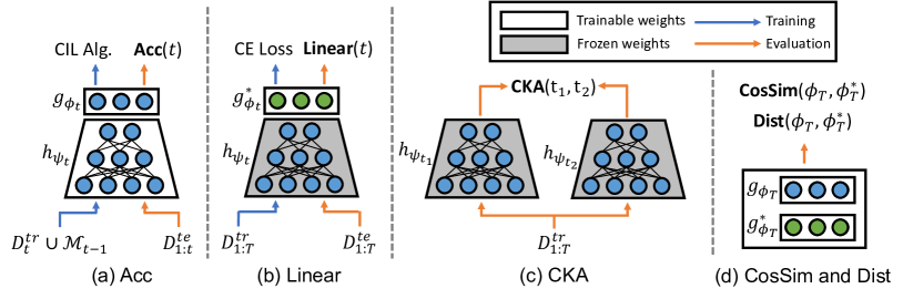
Figure 2: Proposed evaluation methods

3 Proposed Evaluation

3.1 Problem formulation and preliminaries

In this section, we briefly introduce the preliminaries and problem formulation of our paper. We follow the general settings and problem formulation of class-incremental learning (CIL) proposed in previous papers [37, 40, 31].

Notations and settings   We assume a sequential task setting, where $t\in\{1,\dots,T\}$ represents the $t\textsuperscript{th}$ task. Task-specific training and test datasets at task $t$ are denoted as $D_{t}^{\mathrm{tr}}$ and $D_{t}^{\mathrm{te}}$, respectively. Each task-specific dataset $D_{t}=\{(\bm{x}^{(i)}_{t},y^{(i)}_{t})\}^{N}_{i=1}$ consists of $N$ pairs of an input image and its target label. The target label $y_{t}$ is assumed to be sampled from a task-specific class set $\mathcal{C}_{t}$ which are disjoint across different tasks, i.e. $\mathcal{C}_{i}\cap\mathcal{C}_{j}=\emptyset\text{ }\forall i\neq j\in\{1,\dots,T\}$. Exemplar-memory is allocated to store and replay a small number of data instances of previous tasks. More specifically, exemplar-memory which holds data seen until task $t-1$ is denoted as $\mathcal{M}_{t-1}$ and is used for training at task $t$. In this paper, we consider a class-balanced memory which is simple in that it stores equal number of images per class and is known to be efficient.[36, 6, 17, 13]

At task $t$, a classification model $f_{\bm{\theta}_{t}}=(h_{\bm{\psi}_{t}}\circ g_{\bm{\phi}_{t}})$ is trained, where $h_{\bm{\psi}_{t}}$ and $g_{\bm{\phi}_{t}}$ indicates the encoder and the output layer of the model, respectively. In this paper, We consider and compare CIL algorithms that use the cross-entropy (CE) objective function as a main training objective. Note that the model trained with the entire training datasets until task $t$ is denoted as joint which is an oracle case.

In short, $f_{\bm{\theta}_{t}}$ is trained on $D_{t}^{\mathrm{tr}}\cup\mathcal{M}_{t-1}$ for multiple epochs (offline training) at task $t$, and evaluated on $D_{1:t}^{\mathrm{te}}$. In CIL, task ID, an additional supervisory signal, is not provided as it adopts a shared output layer. The single-head configuration of CIL is known to make it more susceptible to catastrophic forgetting in classification performance than TIL [40].

Traditional metrics of CIL   Among various ordinary metrics for CIL, we adopt two general metrics for evaluating the performance of CIL algorithm: Acc${(t)}$ and AvgAcc${(t)}$. Acc${(t)}$ is the test accuracy of $f_{\bm{\theta}_{t}}$ on $D_{1:t}^{\mathrm{te}}$, and AvgAcc${(t)}$ is the average of Acc${(t)}$ from the first task to the $t$-th task, i.e., $\text{{AvgAcc}}{(t)}=\frac{1}{t}\sum_{l=1}^{t}$Acc${(l)}$.

3.2 Evaluation protocol for representation analysis

(1) In-domain evaluation: Linear${(t)}$ and $k$-NN${(t)}$   To compare the improvement of representations learned by CIL algorithms, we borrow the evaluation methods used in representation learning research [44, 15]: Linear probing and $k$-NN classification. As shown in Figure 2 (b), representations of each encoder $h_{\bm{\psi}_{t}}$ is evaluated by freezing the encoder $h_{\bm{\psi}_{t}}$ and conducting a linear evaluation by re-training the final linear layer to obtain an optimal classifier $g^{*}_{\bm{\phi}}$. $k$-NN classifier ($k=20$) is also constructed with the frozen encoder. Note that the entire training dataset of a given CIL scenario, $D_{1:T}^{\mathrm{tr}}$, is used to train the linear layer or to formulate $k$-NN classifier and that the is entire test dataset $D_{1:T}^{\mathrm{te}}$ is used for evaluation.

(2) Out-domain evaluation: CLS${(t)}$   To further evaluate the quality of the learned representations in more generalaspects, we conduct experiments of transfer learning with out-domain datasets as well. We consider three downstream tasks of classification, namely STL-10 [9], CUB200 [41], and resized ($96\times 96$) CIFAR-10 [25]. For each encoder $h_{\bm{\psi}_{t}}$, we perform linear evaluation using each dataset and report their average classification accuracy.

(3) Representation similarity comparison: CKA${(t_{1},t_{2})}$   We compare the degree of changes of learned representations during a task change in CIL from $t_{1}$ to $t_{2}$ by measuring their similarity using CKA [23]. That is, as shown in Figure 2 (c), we measure CKA between $h_{\bm{\psi}_{t_{1}}}$ and $h_{\bm{\psi}_{t_{2}}}$ by using entire training dataset $D_{1:T}^{\mathrm{tr}}$.

(4) Decision boundary comparison   For more detailed analysis for a decision boundary, we propose to conduct comparison between an original classifier layer $g_{\bm{\phi}_{T}}$ and an optimal classifier layer $g^{*}_{\bm{\phi}_{T}}$ trained for linear evaluation, for the final $T$-th task’s model. Let $W\in\mathbb{R}^{D\times C}$ and $W^{*}\in\mathbb{R}^{D\times C}$ are parameters of the classifier layer of $g_{\bm{\phi}_{T}}$ and $g^{*}_{\bm{\phi}_{T}}$, respectively. $D$ denotes the dimension of an output feature of $h_{\bm{\psi}_{T}}$ and $C$ stands for the number of the whole classes. To compare both parameters, we calculate both cosine similarity and $L_{2}$ distance between them as below:

$$\mathrm{\textbf{CosSim}}(\phi_{T},\phi^{*}_{T})=\frac{1}{C}\sum_{i}^{C}\frac{(W_{i})^{\intercal}W^{*}_{i}}{\|W_{i}\|_{2}\|W^{*}_{i}\|_{2}}$$

$$\mathrm{\textbf{Dist}}(\phi_{T},\phi^{*}_{T})=\frac{1}{C}\sum_{i}^{C}\|W_{i}-W^{*}_{i}\|_{2}$$

where $i$ denotes an index of column axis and $W_{i},W^{*}_{i}\in\mathbb{R}^{D}$. Note that, when CosSim$(\phi_{T},\phi^{*}_{T})$ is high and Dist$(\phi_{T},\phi^{*}_{T})$ is low at the same time, the decision boundaries of the original classifier is similar to that of the optimal classifier, given same representations of $h_{\bm{\psi}_{T}}$.

4 Experimental Setup

Baselines   We apply the analyses to a model trained with regularization-based algorithms using exemplars [3, 13, 2, 20] The baseline algorithms used in our experiments and brief descriptions of them are as follows:

In this paper, we mainly focus on regularization-based algorithms using exemplar-memory. These algorithms aim to overcome the trade-off between stability and plasticity of CIL by utilizing regularization designed for fixed model capacity.

1. Finetuning (FT): Finetune a model only using cross-entropy loss with exemplars.

2. MAS [3]: Measures the importance of each weight that constitutes the model using gradients and uses this importance as the strength of regularization to overcome catastrophic forgetting.

3. BiC [42]: Overcomes catastrophic forgetting by performing knowledge distillation from the previously learned model, as in LWF [28]. Additionally, biased prediction issues in the output layer are resolved through post-processing on the prediction score. We also report results of BiC (w/o BC) which indicates results without the bias correction post-processing for output logits.

4. PODNet [13]: Devises a more sophisticated spatial-based distillation loss to balance between learning new classes and forgetting previously learned classes.

5. SSIL [2]: Uses separated softmax and task-wise knowledge distillation to alleviate biased predictions.

6. AFC [20]: Calculates the importance in each feature map and proposes regularization using this importance to learn new knowledge well while preserving previously learned knowledge.

For our experiments, we trained models using the official codes of PODNet, SSIL, and AFC for each algorithm. For BiC, we conducted experiments using the implementation in the official code of PODNet, and for FT and MAS, we conducted experiments using the CIL framework proposed in [31].

CIL scenarios   Experiments are conducted on two CIL scenarios using the ImageNet-100 dataset [12]. The first scenario, denoted as 10-tasks, is the most basic form, consisting of 10 tasks each with 10 classes that are continuously learned. The second scenario, denoted as 11-tasks (with the base task), is a recently considered scenario where 50 classes are learned in the base task (first task), followed by 10 continuous tasks each with 5 classes.

Other settings   For all experiments, we used the ResNet-18  [16] architecture. All the baseline models are trained with the same hyperparameters proposed in the original work.

For additional training required in Linear${(t)}$, we trained the output layer with a mini-batch size of 256 with 30 epochs for in-domain dataset and 100 epochs for out-domain datasets. SGD optimizer with an initial learning rate of 0.1 and momentum of 0.9 and decay rate of 0.0001 was used. We applied a schedule that multiplies the learning rate by 0.1 at {10, 20} and {40, 80} epochs for in-domain and out-domain evaluation, respectively. We conducted experiments for three seeds and report averaged results of them.

5 Experimental Results

5.1 Many SOTA algorithms benefit from strong representation stability

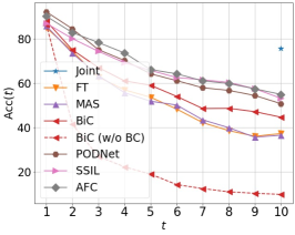
(a) Acc($t$).

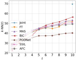
(b) $k$-NN($t$)

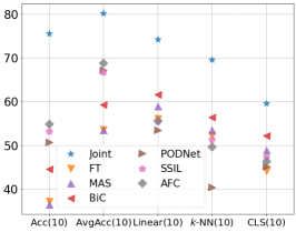
(c) All eval. metrics

Figure 3: Experimental results of the CIL algorithms for the scenario of 10-tasks.

Firstly, our findings on 10-tasks scenario insist that methods that reported high test accuracy not necessarily have encoder with good representation quality.

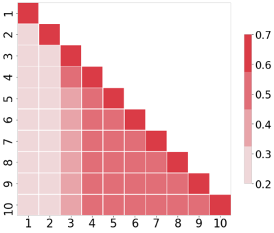
(a) Joint

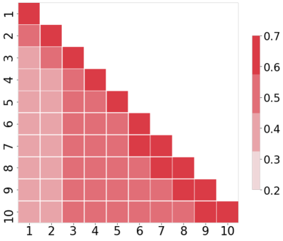
(b) BiC

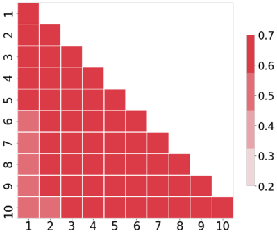
(c) PODNet

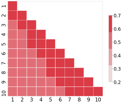
(d) AFC

Figure 4: CKA${(t_{1},t_{2})}$ in 10-tasks scenario for $t_{1},t_{2}\in\{1,\dots,10\}$

In detail, Acc($t$) results for three state-of-the-art algorithms (PODNet, SSIL and AFC) exhibit superior accuracy compared to other baselines at all $t$ in Figure 10(a). However, in Figure 10(b) where $k$-NN($t$) indicates superiority of representation quality, the three algorithms that achieved good results in Figure 10(a) failed to achieve better accuracy than other baselines, and BiC learns the best representation quality. Unlike other baselines that show progress in representation quality as the task increases, note that PODNet which was one of the baseline with the highest Acc($t$) shows poor results, even worse than FT, and seems to converge to certain state. Also, high $k$-NN($t$) of BiC leading to significant improvement in Acc($t$), from BiC(w/o BC) to BiC, aligns with results mentioned in their paper [42]. Figure 10(c) shows results for $t=10$ for all five metrics (numerical values for each result are also provided in Table 1). Similarly, we also observe that state-of-the-art algorithms achieve superior performance in the typical metrics but consistently perform worse than BiC in the three metrics used to evaluate the quality of the learned representation. PODNet also showed the largest gap between the typical metric(Acc($10$)) and the metric used to measure representation quality.

Secondly, poor sequential representation update may result from strong stability. In order to check the connection, we compare the results of representation quality results, Figure 10(b), and CKA results along sequential tasks, Figure 4. Figure 4 shows CKA${(t_{1},t_{2})}$ of Joint, BiC, PODNet, and AFC, which compares the representation similarity between $h_{\bm{\psi}_{t_{1}}}$ and $h_{\bm{\psi}_{t_{2}}}$. For example, CKA($5,1$) and CKA($3,1$) of Joint in Figure 11(a) shows that model encoder at task $5$ is less similar to the initial encoder compared to encoder at task $3$. Later on, Joint learns relatively similar representations to the nearby tasks and finally achieves the best quality representation (as in the Joint result at $t=10$ in Figure 3).

BiC which outperformed other baselines in terms of representation quality shows closest overall CKA result to Joint, but the similarity between the representations of each $t$-th model is slightly higher. On the other hand, Compared to Joint and BiC, state-of-the-art algorithms such as PODNet and AFC show higher CKA across tasks. Moreover, PODNet which had the lowest quality shows high similarity between tasks, which indicates that the model learns new tasks without significantly changing the representations. For CKA results of other baselines, please refer Supplementary Materials.

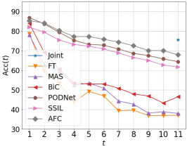
(a) Acc($t$).

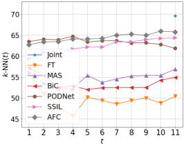
(b) $k$-NN($t$).

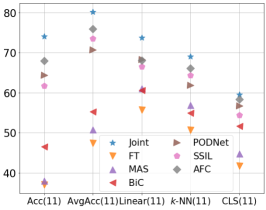
(c) All eval. metrics.

Figure 5: Experimental results of the CIL algorithms for the scenario of 11-tasks.

Considering the CKA experiment results and the comparison with the experiment results in Figure 3, we can infer that state-of-the-art algorithms place great emphasis on maintaining stability in retaining the knowledge of previously learned tasks, which not only prevents significant changes but also limits the ability to learn better quality representations. Furthermore, these experimental results demonstrate that the main argument of the state-of-the-art algorithms, such as PODNet and AFC, which suggest balancing the trade-off between plasticity and stability through the proposed their regularization, is not valid in learned representations.

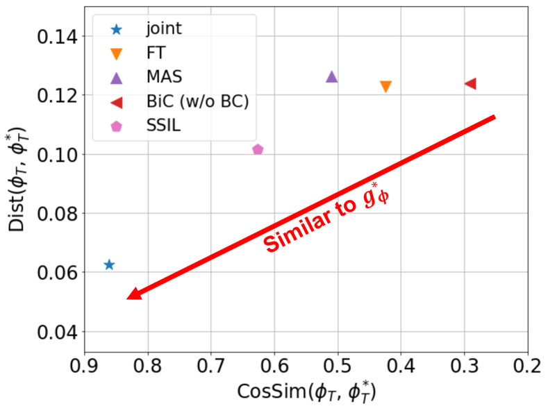
Figure 6: Experimental results of CosSim$(\phi_{T},\phi^{*}_{T})$ and Dist$(\phi_{T},\phi^{*}_{T})$

Lastly, one remaining question is how does the state-of-the-art algorithms(PODNet, SSIL, and AFC) can still achieve high Acc($t$) and AvgAcc($t$) even with poor representations? The answer is in the decision boundary.

Figure 6 compares the similarity between the original classifier learned in last task, i.e.,$g_{\bm{\phi}_{T}}$, and the optimal classifier trained through linear evaluation, i.e., $g^{*}_{\bm{\phi}_{T}}$ using the evaluation metrics introduced in Section 3.2 (4). Since many previous works have already pointed out the severe prediction bias in the classifier of CIL algorithms [42, 4, 2], this evaluation can also show the bias existence in the original classifier.

Note that results for PODNet and AFC does not exist since those algorithms does not use a linear classifier but adopts a elaborately desinged classifier to address the biased prediction problem in the output layer that occurs during CIL. Additionally, for BiC, comparison with Acc($t$) and AvgAcc($t$) of BiC (w/o BC) is necessary since the post-processing of BiC is applied to the logit score, not the classifier weights.

In Figure 6, the joint model which is known as the upperbound shows the highest CosSim$(\phi_{T},\phi^{*}_{T})$ and the lowest Dist$(\phi_{T},\phi^{*}_{T})$. On the other hand, BiC(w/o BC) shows the least similarity to the optimal classifier with given encoder. Also, due to bias resolved classifier, SSIL learns a classifier relatively more closer to the optimal classifier than FT and MAS, which can explain why FT and MAS with relatively better representations achieves lower final accuracy than SSIL and other state-of-the-arts baselines.

Similarly, despite the fact that the models trained by PODNet and AFC may have learned relatively poor representations, we can infer that both algorithms can achieve high final accuracy because they effectively learn the better decision boundary than other baselines.

Evaluation on 11-tasks scenario   Using the proposed representation evaluation protocol, we further evaluate baseline models on a large base task scenarios where stability is highly required. Firstly, Figure 10(d) and 10(e) shows the superiority of state-of-the-art algorithms(PODNet, SSIL, and AFC) both in Acc($t$) and $k$-NN($t$). Not only do they achieve relatively overwhelming accuracy compared to other algorithms, but they also show accuracy that is nearly approaching that of Joint. Similarly, Figure 5(c) demonstrates that these two algorithms show the best results in all metrics. Secondly, cross-task CKA results of large base scenario in Figure 7 show similar results to that of the 10-tasks results in 4. However, unlike PODNet and AFC which enforces strong stability, joint model learns new representation that not only is dissimilar from the representation learned in the previous task but still has good representation quality.

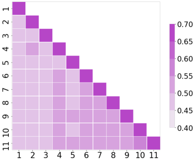
(a) Joint

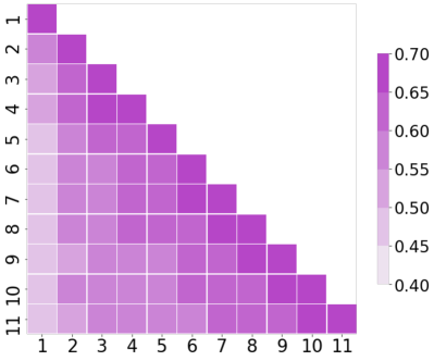
(b) BiC

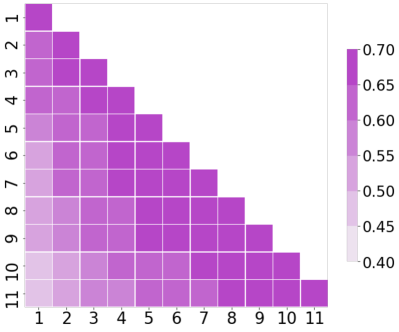
(c) PODNet

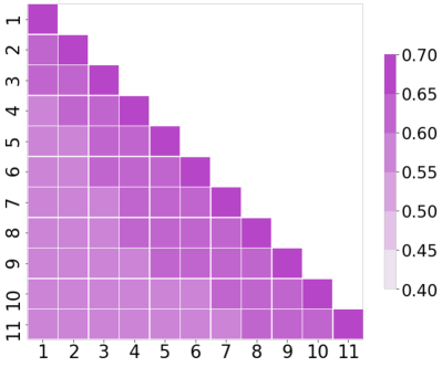
(d) AFC

Figure 7: CKA${(t_{1},t_{2})}$ in 11-tasks scenario for $t_{1},t_{2}\in\{1,\dots,11\}$

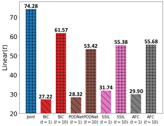
(a) 10-tasks

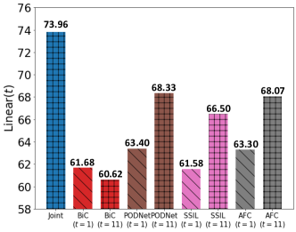
(b) 11-tasks with the base task

Figure 8: Experimental results of Linear($1$) and Linear($T$) for each algorithm.

Based on the results above, firstly, we can experimentally infer that the high test accuracy achieved by state-of-the-art CIL algorithms does not imply good representation learning of sequential tasks. Secondly, better decision boundary determination is important and it can sometimes lead to better prediction even with representation with inferior quality. Lastly, the state-of-the-art algorithms(PODNet, SSIL, and AFC) actually focus more on maintaining stability while learning a series of tasks. As a result, the scenario of learning on a large base task is advantageous for these algorithms because simply maintaining knowledge learned in the initial task leads to superior performance regarding all the proposed metrics. In this regard, the question naturally arises as to whether each algorithm learns the base task (the first task) similarly, especially on the scenario with large base task.

Table 1: Experimental results for 10- and 11-tasks scenarios.

Alg.	10-tasks						11-tasks (with the base task)
	Typical Metrics		In-domain Eval.			Out-domain Eval.	Typical Metrics		In-domain Eval.			Out-domain Eval.
	Acc($10$)	Avg($10$)	Linear($0$)	Linear($10$)	$k$-NN($10$)	CLS($10$)	Acc($11$)	Avg($11$)	Linear($0$)	Linear($11$)	$k$-NN($11$)	CLS($11$)
Joint	75.56	80.23	-	74.28	69.62	59.57	75.40	84.23	-	73.96	74.42	59.80
FT	37.20	53.48	33.12	56.08	52.04	44.09	37.01	47.35	61.22	56.12	56.12	41.72
MAS	36.48	53.55	32.66	58.94	53.38	48.91	38.00	50.85	60.62	61.08	61.08	44.79
BiC	44.60	59.28	27.22	61.58	56.36	52.20	46.50	55.31	61.67	60.61	63.40	51.71
PODNet	50.70	66.70	28.32	53.42	40.26	45.09	64.40	73.48	63.40	68.33	61.86	56.67
SSIL	53.14	67.12	31.74	55.38	50.98	47.28	61.72	70.41	61.58	66.50	61.48	54.39
AFC	54.90	68.83	29.90	55.68	49.33	46.39	67.90	75.89	63.30	68.07	63.30	58.38

5.2 The first task’s model may learn different quality of representation

Most CIL algorithms aim to find their hyperparameters that maximize the average test accuracy for a given dataset and CIL scenario, and evaluate their algorithm’s relative superiority to other baselines. During this process, hyperparameters are typically set without special consideration for the base task, and only the result after learning the entire task sequence is taken into account. However, since the settings used for utilizing CIL algorithm may differ for each algorithm (e.g., optimizer, epochs, etc.), the results of training the base task model, which is learned as if it were a single task, can vary regardless of the CIL algorithm. In short, training details of first tasks differ from each algorithms, which leads to different first task model.

To investigate consequential effects of this issue, we compared the linear evaluation results of the first task model and the final task model trained by each algorithm in the 10-tasks and 11-tasks scenarios in Figure 8. From this figure, we can observe the following experimental results. First, even it was trained in the same scenario with the same dataset (ImageNet-100), the linear evaluation results of the first task differ among algorithms, i.e., different Linear($1$) by algorithms in the figure. Second, in the 11-tasks scenario, each algorithm’s first task model already starts with a superior representation learned, compared to the linear evaluation results of the Joint model (e.g., the difference between the Joint model’s Linear($11$) result and each algorithm’s Linear($1$) result is within 10%). Lastly, the improvement achieved by the state-of-the art algorithms in representation are similar. That is, the difference in linear evaluation results between the last task model and the first task model (Linear($T$) - Linear($1$)) are about $25\%$ and $5\%$ for those algorithms in each scenarios. As a result, it’s hard to compare superiority of each algorithms with different first task representation.

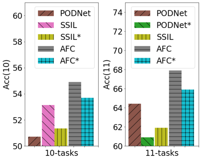
Figure 9: Experimental results with a unified first task model.

5.3 Unifying first task model results in different final performance

In the previous section, we experimentally confirmed that first task models learned by each algorithm in the same scenario using the same dataset can have different representation qualities. Given that the first task is typically learned similarly to a single task and not closely related to CIL algorithms, comparing algorithms learned with different representation qualities may not be objective.

To address this issue, we conducted experiments where we trained subsequent tasks with a unified performance difference of 1% in Linear($1$) in each scenario. For this purpose, in the 10-tasks scenario, we reduced the first training epoch of SSIL and AFC to match the linear evaluation results of the PODNet’s first task, and in the 11-tasks scenario, we trained subsequent tasks by matching the linear evaluation results of the PODNet and AFC’s first task to SSIL.

Figure 9 and Table 2 show the results of learning the 10- and 11-tasks scenarios starting from a unified first task model. Specifically, Figure 9 shows the changes in results in the typical metric, Acc($T$). In the figure, * represents the experimental results for using the unified first task model. From the experimental results, we observed that when the first task model was unified, the performance of each algorithm decreased in both scenarios. In the 10-tasks scenario, SSIL* and AFC* showed a performance decrease of 1-2% in Acc($10$) compared to the previous results, and for SSIL*, the difference in Acc(10) with PODNet decreased from about 4% to about 0.6%. Additionally, in the 11-tasks scenario, PODNet* and AFC* decreased by 2-4% compared to the previous results. As a result, PODNet achieved about 3% higher accuracy than SSIL, but PODNet* achieved about 1% lower accuracy instead.

Furthermore, by comparing Table 1 and Table 2, we also observe changes in the quality of representations. In particular, in the 11-tasks scenario, we observe that the representation quality of the final model was greatly affected by the changes in the first task (base task) model. For example, both PODNet and AFC started learning from a model that had decreased by about 2% at Linear($1$), and the results showed a significant performance decrease of about 4% at Linear($11$) and 2-6% at $k$-NN($11$) and CLS($11$).

Table 2: Experimental results with a unified first task model. * denotes using the unified first task model.

Alg.	10-tasks
	Acc($T$)	Avg($10$)	Linear($0$)	Linear($10$)	$k$-NN($10$)	CLS($10$)
SSIL*	51.34	65.74	28.48	54.54	52.26	45.28
AFC*	53.70	67.85	28.48	51.02	46.82	43.28
Alg.	11-tasks (with the base task)
	Acc($11$)	Avg($11$)	Linear($0$)	Linear($11$)	$k$-NN($11$)	CLS($11$)
PODNet*	60.90	70.11	61.28	63.28	55.26	51.67
AFC*	65.90	74.48	61.24	64.34	61.70	56.80

In conclusion, most CIL algorithms focus on maintaining stability, so the quality of representation learned from the first task model can have a significant impact on the overall performance evaluation, but there has not been much deep consideration on this issue. Therefore, based on our proposed experimental analysis, we have shown that it is necessary to unify the representation quality of the first task model for objective evaluation of CIL algorithms.

6 Discussion

What are the main findings of the experiments?   We discovered two key findings through analyzing and evaluating CIL algorithms. Firstly, state-of-the-art algorithms that achieve high test accuracy may learn representations of poorer quality or ones that do not improve significantly compared to other baselines. This is because most algorithms prioritize achieving high stability, which may lead to learning relatively poor representations but setting decision boundaries well. Therefore, high test accuracy does not necessarily indicate high-quality representation learning. Secondly, the quality of the representation of the first task model that each algorithm learns may vary and can have a significant impact on the final performance evaluation.

Why is the evaluation for representations necessary?   If we do not evaluate the representation of models trained by each algorithm, algorithms that set decision boundaries better, even if they learn the worse representation, will be evaluated as superior algorithms. This is not only inaccurate in evaluating algorithms objectively but also, if not pursuing to improve the representation, the upper bound of each algorithm will be the linear evaluation result of the currently trained model rather than Joint model. This does not align with the ultimate goal of CIL, which is to achieve the performance of the Joint model in class incremental learning scenarios.

What steps should we take to move forward?   Taking into account all the findings of this paper, we propose the following suggestions for a more objective evaluation of CIL algorithms and for the development of more advanced CIL algorithms:

• First, we recommend evaluating the representation quality of the models learned by CIL algorithms, as algorithms should strive not only to achieve high average test accuracy but also learn improved representation quality.

• Second, since the scenario of learning the base task favors algorithms that prioritize stability, it is essential to also consider the experimental results of learning an equal number of classes to evaluate the stability and plasticity of the algorithms simultaneously.

• Third, to compare and evaluate the performance of different algorithms fairly, it is necessary to consider the quality of the representation of the first task model, as this may vary and significantly affect the final performance.

Appendix A Detailed Experimental Settings

Experimental settings of CIL algorithm   We achieved the result of CIL algorithms, FT, MAS [3] and LWF [28] by implementing the CIL framework code proposed by [31]. We did not modify the default hyperparameters for each algorithm. We trained these algorithms for 100 epochs for each task using the SGD optimizer with an initial learning rate of 0.1, momentum of 0.9, and weight decay of 0.0001. We also set a learning rate schedule that dropped the learning rate by a factor of 0.1 at 40 and 80 epochs, respectively. For all experiments, we used a mini-batch size of 256. We employed random sampling as the sampling algorithm for the exemplar memory.

We evaluated several state-of-the-art CIL algorithms, including PODNet [13], SSIL [2], and AFC [20]. To ensure fair comparisons, we run the official code for each algorithm without modifying not only the default hyperparameters but also other settings for training, such as learning rate, epochs, and mini-batch size. Furthermore, we obtained experimental results for LUCIR [17] and BiC [42] using the code implemented in [13], also without any modification.

Linear evaluation   We retrained the output layer while freezing the encoder. Specifically, we trained the output layer for 30 epochs using a mini-batch size of 256, and utilized the SGD optimizer with an initial learning rate of 0.1, momentum of 0.9, and weight decay of 0.0001. We implemented a learning rate schedule, which decreased the learning rate by a factor of 0.1 at the 40th and 80th epochs, respectively.

$k$-NN evaluation   For all experiments, we utilized the $k$-NN implementation ($k=20$) provided by scikit-learn [35]. In the classification process, we first fit the $k$-NN with the outputs of the encoder for the given inputs, and subsequently classify the test data using the $k$-NN classifier.

Three downstream tasks   We selected CIFAR-10 [25], STL-10 [9], and CUB-200 [41] as downstream tasks for out-of-domain evaluation. For CIFAR-10, we randomly selected 5,000 training images from the entire training dataset and resized the input images to $96\times 96$ pixels. For STL-10 and CUB-200, we used the entire training dataset and maintained their original image sizes. We trained only a newly added output layer while freezing the encoder. For CIFAR-10 and CUB-200, we trained the output layer for 100 epochs using a mini-batch size of 128 and used SGD optimizer with an initial learning rate of 0.1, a momentum of 0.9, and a weight decay of 0.0001. We set the learning rate schedule to drop the learning rate by a factor of 0.1 at 40 and 80 epochs, respectively. In the case of STL-10, we changed the number of epochs to 10 and the initial learning rate to 0.005.

Experimental settings for unifying the base task’s model   To unify the representation quality of the first task, we only reduced the number of epochs for the first task training of CIL algorithms that learn relatively better representations than others. The used number of training epochs for the first task is shown in Table 3.

Table 3: Experimental results for 10- and 11-tasks scenarios.

	10-tasks		11-tasks
	SSIL	AFC	PODNet	AFC
First task Epochs	50	45	60	45

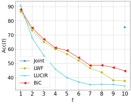
(a) 10-tasks, Acc($t$).

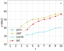
(b) 10-tasks, $k$-NN($t$)

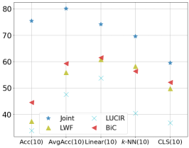
(c) 10-tasks, All eval. metrics

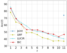
(d) 11-tasks, Acc($t$).

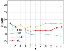
(e) 11-tasks, [$k$-NN($t$)

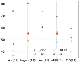
(f) 11-tasks, All eval. metrics

Figure 10: Additional experimental results of LWF and LUCIR for the scenario of 10-tasks and 11-tasks.

Appendix B Analysis for Output Layer of PODNet and AFC

To reduce biased predictions in class-incremental learning (CIL), PODNet proposed local similarity classifier based on the cosine classifier, which utilizes a learnable scaling parameter $\eta$ and $K$ multiple proxies per class to compute the cosine similarity (also, AFC simply applied this as a basic classifier). To perform the decision boundary comparison proposed in the manuscript, the optimal classifier of the classifier must be obtained. However, there are some issues to get the optimal classifier for the local similarity classifier. First, it is difficult to find the optimal classifier due to the influence of the learnable scaling parameter $\eta$, which results in different learned scaling parameters for CIL and linear evaluation scenarios, leading to different trained classifier weights. Second, using $K$ multiple proxies is beneficial for reducing biased predictions in the CIL scenario, but it is not helpful to learn the optimal classifier for the linear evaluation, leading to suboptimal performance. Therefore, we could not perform the decision boundary comparison for PODNet and AFC due to these limitations.

Nevertheless, we can easily infer that, based on Figures 3 and 6 in the manuscript, the reason why AFC and PODNet were able to achieve superior Acc($t$) (and also AvgAcc($t$)) compared to other baselines, despite learning poor representations, is that these algorithms learned better decision boundaries than others. We believe that there doesn’t seem to be any other reason to explain this phenomenon, except for the above inference.

Appendix C Additional Experimental Results

C.1 Experimental analysis for other CIL algorithms

In our experiment using the ImageNet-100 dataset, we conducted additional experiments on LWF and LUCIR, and the results are shown in Figure 10. The results for BiC were added for comparison and are consistent with the results in the manuscript. We were able to confirm experimental results similar to the findings in the manuscript in two scenarios (10-tasks and 11-tasks). Firstly, since the learning of the BiC encoder is carried out through a form of knowledge distillation similar to LWF, the evaluation results for representation quality between LWF and BiC showed no significant difference. Secondly, in the case of LUCIR, although it achieved higher Acc($t$) and AvgAcc($t$) than LWF in the situation of learning from the base model (11-tasks), it was found that the representation quality learned by this algorithm was significantly inferior to LWF.

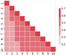
(a) FT (10-tasks)

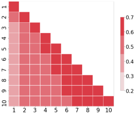
(b) MAS (10-tasks)

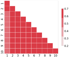
(c) SSIL (10-tasks)

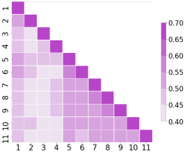
(d) FT (11-tasks)

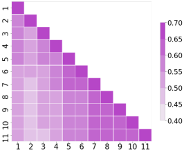
(e) MAS (11-tasks)

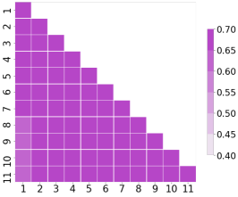
(f) SSIL (11-tasks)

Figure 11: CKA${(t_{1},t_{2})}$ in 10-tasks and 11-tasks scenario.

(a) Acc($t$).

(b) $k$-NN($t$)

(c) All eval. metrics

Figure 12: Additional experimental results with CIFAR-100 for the scenario of 10-tasks.

C.2 CKA results for other CIL algorithms

Figure 11 shows the CKA${(t_{1},t_{2})}$ results for other algorithms in the experiment using ImageNet-100. In the case of 10-tasks, first, FT and MAS show results similar to the Joint in the manuscript. Second, SSIL maintains a relatively strong similarity. Through this, we can further confirm that each SOTA algorithm focuses on stability to prevent significant changes in representation, leading to poorer representation learning compared to FT and MAS in the 10-tasks scenario. In the case of 11-tasks, since a relatively large amount of knowledge (half of the total class number) is learned in the first task, algorithms that focus on stability can achieve relatively superior results. Taking this into account, FT and MAS show significant changes in representation, while SSIL does not, showing a similar trend to the evaluation results for representation quality for each algorithm (See Figure 5 of the manuscript).

C.3 Experimental analysis with CIFAR-100

To investigate whether the analysis results proposed in the paper are dataset-dependent, we conducted CIL experiments using CIFAR-100 for the 10-tasks scenario. We used five representative algorithms (FT, BiC, PODNet, SSIL, and AFC) and conducted experiments with their reported default hyperparameters. All experiments were conducted using the ResNet-18 model, and for SSIL, which has no experiments on CIFAR-100 in the their paper, we applied the same number of epochs (160) used for training in PODNet and AFC. Additionally, we only conducted in-domain evaluation.

Figure 12 shows the experimental results, and we obtained analysis results similar to those of ImageNet-100 in the manuscript. First, we confirmed that AFC and SSIL achieved relatively superior Acc($t$) and AvgAcc($t$), but the representations they learned are inferior to those learned by BiC. Second, we observed that PODNet learned significantly worse representations compared to other algorithms on CIFAR-100.

Based on this, we can confirm that the experimental analysis we have conducted is not dataset-dependent, but rather that each algorithm focuses heavily on stability, which leads to learning the worse representation quality despite achieving high accuracy.

References

- [1] Hongjoon Ahn, Sungmin Cha, Donggyu Lee, and Taesup Moon. Uncertainty-based continual learning with adaptive regularization. In Advances in Neural Information Processing Systems (NeurIPS), pages 4394–4404, 2019.
- [2] Hongjoon Ahn, Jihwan Kwak, Subin Lim, Hyeonsu Bang, Hyojun Kim, and Taesup Moon. Ss-il: Separated softmax for incremental learning. In Proceedings of the IEEE/CVF International Conference on Computer Vision, pages 844–853, 2021.
- [3] Rahaf Aljundi, Francesca Babiloni, Mohamed Elhoseiny, Marcus Rohrbach, and Tinne Tuytelaars. Memory aware synapses: Learning what (not) to forget. In Proceedings of the European Conference on Computer Vision (ECCV), pages 139–154, 2018.
- [4] Eden Belouadah and Adrian Popescu. Il2m: Class incremental learning with dual memory. In Proceedings of the IEEE/CVF International Conference on Computer Vision, pages 583–592, 2019.
- [5] Yoshua Bengio, Yann Lecun, and Geoffrey Hinton. Deep learning for ai. Communications of the ACM, 64(7):58–65, 2021.
- [6] Francisco M Castro, Manuel J Marín-Jiménez, Nicolás Guil, Cordelia Schmid, and Karteek Alahari. End-to-end incremental learning. In Proceedings of the European conference on computer vision (ECCV), pages 233–248, 2018.
- [7] Sungmin Cha, Hsiang Hsu, Taebaek Hwang, Flavio Calmon, and Taesup Moon. {CPR}: Classifier-projection regularization for continual learning. In International Conference on Learning Representations, 2021.
- [8] Arslan Chaudhry, Puneet K Dokania, Thalaiyasingam Ajanthan, and Philip HS Torr. Riemannian walk for incremental learning: Understanding forgetting and intransigence. In Proceedings of the European Conference on Computer Vision (ECCV), pages 532–547, 2018.
- [9] Adam Coates, Andrew Ng, and Honglak Lee. An analysis of single-layer networks in unsupervised feature learning. In Proceedings of the fourteenth international conference on artificial intelligence and statistics, pages 215–223. JMLR Workshop and Conference Proceedings, 2011.
- [10] MohammadReza Davari, Nader Asadi, Sudhir Mudur, Rahaf Aljundi, and Eugene Belilovsky. Probing representation forgetting in supervised and unsupervised continual learning. In Proceedings of the IEEE/CVF Conference on Computer Vision and Pattern Recognition, pages 16712–16721, 2022.
- [11] Matthias Delange, Rahaf Aljundi, Marc Masana, Sarah Parisot, Xu Jia, Ales Leonardis, Greg Slabaugh, and Tinne Tuytelaars. A continual learning survey: Defying forgetting in classification tasks. IEEE Transactions on Pattern Analysis and Machine Intelligence, 2021.
- [12] Jia Deng, Wei Dong, Richard Socher, Li-Jia Li, Kai Li, and Li Fei-Fei. Imagenet: A large-scale hierarchical image database. In 2009 IEEE conference on computer vision and pattern recognition, pages 248–255. Ieee, 2009.
- [13] Arthur Douillard, Matthieu Cord, Charles Ollion, Thomas Robert, and Eduardo Valle. Podnet: Pooled outputs distillation for small-tasks incremental learning. In Computer Vision–ECCV 2020: 16th European Conference, Glasgow, UK, August 23–28, 2020, Proceedings, Part XX 16, pages 86–102. Springer, 2020.
- [14] Enrico Fini, Victor G Turrisi da Costa, Xavier Alameda-Pineda, Elisa Ricci, Karteek Alahari, and Julien Mairal. Self-supervised models are continual learners. In Proceedings of the IEEE/CVF Conference on Computer Vision and Pattern Recognition, pages 9621–9630, 2022.
- [15] Kaiming He, Haoqi Fan, Yuxin Wu, Saining Xie, and Ross Girshick. Momentum contrast for unsupervised visual representation learning. In Proceedings of the IEEE/CVF conference on computer vision and pattern recognition, pages 9729–9738, 2020.
- [16] Kaiming He, Xiangyu Zhang, Shaoqing Ren, and Jian Sun. Deep residual learning for image recognition. In Proceedings of the IEEE conference on computer vision and pattern recognition, pages 770–778, 2016.
- [17] Saihui Hou, Xinyu Pan, Chen Change Loy, Zilei Wang, and Dahua Lin. Learning a unified classifier incrementally via rebalancing. In Proceedings of the IEEE/CVF Conference on Computer Vision and Pattern Recognition, pages 831–839, 2019.
- [18] Ching-Yi Hung, Cheng-Hao Tu, Cheng-En Wu, Chien-Hung Chen, Yi-Ming Chan, and Chu-Song Chen. Compacting, picking and growing for unforgetting continual learning. Advances in Neural Information Processing Systems, 32, 2019.
- [19] Sangwon Jung, Hongjoon Ahn, Sungmin Cha, and Taesup Moon. Continual learning with node-importance based adaptive group sparse regularization. In Advances in Neural Information Processing Systems (NeurIPS), volume 33, pages 3647–3658. Curran Associates, Inc., 2020.
- [20] Minsoo Kang, Jaeyoo Park, and Bohyung Han. Class-incremental learning by knowledge distillation with adaptive feature consolidation. arXiv preprint arXiv:2204.00895, 2022.
- [21] Diederik P Kingma and Jimmy Ba. Adam: A method for stochastic optimization. arXiv preprint arXiv:1412.6980, 2014.
- [22] James Kirkpatrick, Razvan Pascanu, Neil Rabinowitz, Joel Veness, Guillaume Desjardins, Andrei A Rusu, Kieran Milan, John Quan, Tiago Ramalho, Agnieszka Grabska-Barwinska, et al. Overcoming catastrophic forgetting in neural networks. Proceedings of the national academy of sciences, 114(13):3521–3526, 2017.
- [23] Simon Kornblith, Mohammad Norouzi, Honglak Lee, and Geoffrey Hinton. Similarity of neural network representations revisited. In International Conference on Machine Learning, pages 3519–3529. PMLR, 2019.
- [24] Simon Kornblith, Jonathon Shlens, and Quoc V Le. Do better imagenet models transfer better? In Proceedings of the IEEE/CVF conference on computer vision and pattern recognition, pages 2661–2671, 2019.
- [25] Alex Krizhevsky, Geoffrey Hinton, et al. Learning multiple layers of features from tiny images. 2009.
- [26] Yann LeCun, Yoshua Bengio, and Geoffrey Hinton. Deep learning. nature, 521(7553):436–444, 2015.
- [27] Soochan Lee, Junsoo Ha, Dongsu Zhang, and Gunhee Kim. A neural dirichlet process mixture model for task-free continual learning. arXiv preprint arXiv:2001.00689, 2020.
- [28] Zhizhong Li and Derek Hoiem. Learning without forgetting. IEEE transactions on pattern analysis and machine intelligence, 40(12):2935–2947, 2017.
- [29] Divyam Madaan, Jaehong Yoon, Yuanchun Li, Yunxin Liu, and Sung Ju Hwang. Representational continuity for unsupervised continual learning. In International Conference on Learning Representations, 2022.
- [30] Arun Mallya and Svetlana Lazebnik. Packnet: Adding multiple tasks to a single network by iterative pruning. In The IEEE Conference on Computer Vision and Pattern Recognition (CVPR), June 2018.
- [31] Marc Masana, Xialei Liu, Bartlomiej Twardowski, Mikel Menta, Andrew D Bagdanov, and Joost van de Weijer. Class-incremental learning: survey and performance evaluation on image classification. arXiv preprint arXiv:2010.15277, 2020.
- [32] Martial Mermillod, Aurélia Bugaiska, and Patrick Bonin. The stability-plasticity dilemma: Investigating the continuum from catastrophic forgetting to age-limited learning effects. Frontiers in psychology, 4:504, 2013.
- [33] Seyed Iman Mirzadeh, Mehrdad Farajtabar, Razvan Pascanu, and Hassan Ghasemzadeh. Understanding the role of training regimes in continual learning. Advances in Neural Information Processing Systems, 33:7308–7320, 2020.
- [34] German I Parisi, Ronald Kemker, Jose L Part, Christopher Kanan, and Stefan Wermter. Continual lifelong learning with neural networks: A review. Neural Networks, 113:54–71, 2019.
- [35] Fabian Pedregosa, Gaël Varoquaux, Alexandre Gramfort, Vincent Michel, Bertrand Thirion, Olivier Grisel, Mathieu Blondel, Peter Prettenhofer, Ron Weiss, Vincent Dubourg, et al. Scikit-learn: Machine learning in python. the Journal of machine Learning research, 12:2825–2830, 2011.
- [36] Ameya Prabhu, Philip HS Torr, and Puneet K Dokania. Gdumb: A simple approach that questions our progress in continual learning. In European Conference on Computer Vision, pages 524–540. Springer, 2020.
- [37] Sylvestre-Alvise Rebuffi, Alexander Kolesnikov, Georg Sperl, and Christoph H Lampert. icarl: Incremental classifier and representation learning. In Proceedings of the IEEE conference on Computer Vision and Pattern Recognition, pages 2001–2010, 2017.
- [38] Andrei A Rusu, Neil C Rabinowitz, Guillaume Desjardins, Hubert Soyer, James Kirkpatrick, Koray Kavukcuoglu, Razvan Pascanu, and Raia Hadsell. Progressive neural networks. arXiv preprint arXiv:1606.04671, 2016.
- [39] Jonathan Schwarz, Wojciech Czarnecki, Jelena Luketina, Agnieszka Grabska-Barwinska, Yee Whye Teh, Razvan Pascanu, and Raia Hadsell. Progress & compress: A scalable framework for continual learning. In International Conference on Machine Learning (ICML), pages 4528–4537, 2018.
- [40] Gido M Van de Ven and Andreas S Tolias. Three scenarios for continual learning. arXiv preprint arXiv:1904.07734, 2019.
- [41] Catherine Wah, Steve Branson, Peter Welinder, Pietro Perona, and Serge Belongie. The caltech-ucsd birds-200-2011 dataset. 2011.
- [42] Yue Wu, Yinpeng Chen, Lijuan Wang, Yuancheng Ye, Zicheng Liu, Yandong Guo, and Yun Fu. Large scale incremental learning. In Proceedings of the IEEE/CVF Conference on Computer Vision and Pattern Recognition, pages 374–382, 2019.
- [43] Lu Yu, Bartlomiej Twardowski, Xialei Liu, Luis Herranz, Kai Wang, Yongmei Cheng, Shangling Jui, and Joost van de Weijer. Semantic drift compensation for class-incremental learning. In Proceedings of the IEEE/CVF Conference on Computer Vision and Pattern Recognition, pages 6982–6991, 2020.
- [44] Jure Zbontar, Li Jing, Ishan Misra, Yann LeCun, and Stéphane Deny. Barlow twins: Self-supervised learning via redundancy reduction. In International Conference on Machine Learning, pages 12310–12320. PMLR, 2021.