An Improved Normed-Deformable Convolution
for Crowd Counting

Abstract

In recent years, crowd counting has become an important issue in computer vision. In most methods, the density maps are generated by convolving with a Gaussian kernel from the ground-truth dot maps which are marked around the center of human heads. Due to the fixed geometric structures in CNNs and indistinct head-scale information, the head features are obtained incompletely. Deformable convolution is proposed to exploit the scale-adaptive capabilities for CNN features in the heads. By learning the coordinate offsets of the sampling points, it is tractable to improve the ability to adjust the receptive field. However, the heads are not uniformly covered by the sampling points in the deformable convolution, resulting in loss of head information. To handle the non-uniformed sampling, an improved Normed-Deformable Convolution (i.e.,NDConv) implemented by Normed-Deformable loss (i.e.,NDloss) is proposed in this paper. The offsets of the sampling points which are constrained by NDloss tend to be more even. Then, the features in the heads are obtained more completely, leading to better performance. Especially, the proposed NDConv is a light-weight module which shares similar computation burden with Deformable Convolution. In the extensive experiments, our method outperforms state-of-the-art methods on ShanghaiTech A, ShanghaiTech B, UCF_QNRF, and UCF_CC_50 dataset, achieving 61.4, 7.8, 91.2, and 167.2 MAE, respectively. The code is available at https://github.com/bingshuangzhuzi/NDConv.

I Introduction

Due to the expansion of worldwide population and the acceleration of urbanization, the probability of crowd massing has increased in recent years. In some scenarios, stampedes and large-scale events pose a hazard to public safety that should be prevented all the time. In order to keep the public safety, crowd counting gains considerable attention in the field of computer vision. Furthermore, the foundation of hardware for crowd counting is provided by the advancement of remote-distance intellectualized cameras [5, 6, 7],[38, 39, 40, 41]. Therefore, there are many researches based on crowd counting[1, 2, 3] which estimate the amount of crowd in campuses, shopping malls, and train stations accurately.

Currently, the previous crowd counting algorithms can be classified into three categories: tracking-based

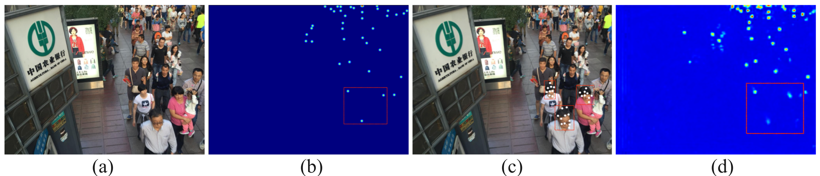
Figure 1: Visualization of the offsets and density maps predicted from models trained with DConv. (a) is one of the input images in ShanghaiTech B dataset, (b) is the ground_truth, the offsets are visualized in (c), and the estimated density map is shown in (d). Due to the sampling points are uniformed in (c), (d) shows less regular Gaussian blobs.

methods[8, 9], feature-based regression methods[10, 11], and CNN-based methods[12, 13, 14]. By comparison, CNN-based methods show their superiority in higher accuracy, efficiency, and robustness. Although great progress has been made in prior works of crowd counting implemented by convolutional neural networks (CNNs), the inability of CNNs adapting to alterations of head-scale[35, 36, 37] is still a barrier, restricting the enhancement of counting accuracy. The methods[15, 16] based on multi-scale feature fusion attempt to address above-mentioned problems. However, there are also some obstacles. Firstly, due to the limitation that parameters of network and computational time balloon along with the increase of the scales of features, the training time is unbearable. In addition, only a few works pay attention on the mechanisms to handle geometric transformations.

To address the above-mentioned problems, a module called Deformable Convolution(i.e.,DConv)[17, 18] is proposed to enhance the CNNs’ capability of modeling geometric transformations by adding additional offsets. However, as shown in the Fig. 1 , it is still non-trivial to sample the head features correctly and uniformly due to the uncontrollable offsets of sampling points in the above-mentioned versions. Based on the preceding discussion, we argue that it is difficult to sample uniformly by simply integrating Deformable Convolution into the network. Therefore, in this work, we attempt to address the problem of non-uniform sampling with extra loss.

Since the offsets are not constrained in DConv, the sampling region is irregular, making it difficult to sample the features of heads uniformly. Thus, a novel Normed-Deformable Convolution (i.e.,NDConv) which is implemented by Normed-Deformable loss (i.e.,NDloss) is proposed to address the forementioned problem. The offsets of sampling points are controlled by NDloss. As a result, the features in the heads are captured more completely, leading to better performance. In our implementation, CSRNet[19] is adopted as the backbone. As the baseline, the last dilated convolution layer is replaced with Deformable Convolution which is denoted as CSRNet$\star$. Without bells and whistles, by replacing the Deformable Convolution in CSRNet$\star$ with the proposed NDConv, we achieve better performance (i.e., $5.5\%$, $13.3\%$, $4.5\%$ and $4.2\%$ improvement in MAE(Mean Absolute Error) on ShanghaiTech A, ShanghaiTech B, UCF_QRNF, and UCF_CC_50.)

In summary, the main contributions of this paper are three-fold.

• Comparing with conventional Deformable Convolution, a novel Normed-Deformable Convolution (i.e.,NDConv) is proposed in which the sampling points tend to be more uniformly spread over the head, resulting in more adequate feature aggregation.

• Our NDconv encourages more thoughts that shape priors should be intergrated into the Deformable Convolution by constraining the sampling offsets.

• Based on the proposed NDConv, better performance is achieved on several crowd counting datasets than the state-of-the-art methods.

II Proposed Method

In this section, the definition and principles of Normed-Deformable Loss are described firstly, and then the architecture of the training network is presented.

II-A Normed-Deformable Loss

Given a convolution of kernel size $3\times 3$ for example, the standard nine sampling points respectively denoted as $a,b,c,d,e,f,g,h,i$ lie strictly on the grid. For Deformable Convolution, due to the existence of sampling offsets, the sampling points $a,b,c,d,e,f,g,h,i$ move to $A,B,C,D,E,F,G,H,I$, respectively. In this case, the offsets are two-dimensional and are recorded as $(\Delta A_{x},\Delta A_{y}),\cdots,(\Delta I_{x},\Delta I_{y})$, where we have $\mathrm{\it A}=\Delta{\it A}+{\it a},\cdots,\mathrm{\it I}=\Delta{\it I}+{\it i}$.

Fig. 2(a) visualizes a typical case of sampling points in DConv, the sampling points travel almost randomly due to no explicit constraints applied on the corresponding offsets. Obviously, the sampling positions fail to evenly cover the head region, leading to inadequate feature aggregation. By considering the prior that the head tends to be in the shape of ellipse, an intuitive thought is constraining the offsets of sampling points to be in accordance with the prior, making the feature aggregation more sufficient.

Here, we make a simplification on the prior. Specifically, the ellipse is decoupled into four parallelograms, i.e.,$ABED$, $CBEF$, $GHED$, $IHEF$, depicted in Fig. 2(b). Before we build the corresponding loss for these parallelograms, three restrictions should be constructed to make the whole sampling points more reasonable. (i) The central sampling point $E$ should be close to $e$, which is intuitive. (ii) $D$ and $F$ share the same distance away from $e$, and both $D$ and $F$ should be close to $x$-axis. (iii) Similarly, $B$ and $H$ should be the same distance away from $e$, and both $B$ and $H$ should be close to $y$-axis.

For restriction (i), we have:

$$\mathcal{L}_{e}=\left\|\Delta E_{x}\right\|_{2}^{2}+\left\|\Delta E_{y}\right\|_{2}^{2}\\$$ (1)

For restriction (ii), we have:

$$\mathcal{L}_{hor}=\left\|\Delta D_{x}+\Delta F_{x}\right\|_{2}^{2}+\left\|\Delta D_{y}\right\|_{2}^{2}+\left\|\Delta F_{y}\right\|_{2}^{2}$$ (2)

And for restriction (iii), we have:

$$\mathcal{L}_{vec}=\left\|\Delta B_{y}+\Delta H_{y}\right\|_{2}^{2}+\left\|\Delta B_{x}\right\|_{2}^{2}+\left\|\Delta H_{x}\right\|_{2}^{2}$$ (3)

Finally, we constrian the four diagnoal points $A$, $C$, $G$, $I$, making them close to the four parallelograms, i.e.,$ABED$, $CBEF$, $GHED$, $IHEF$:

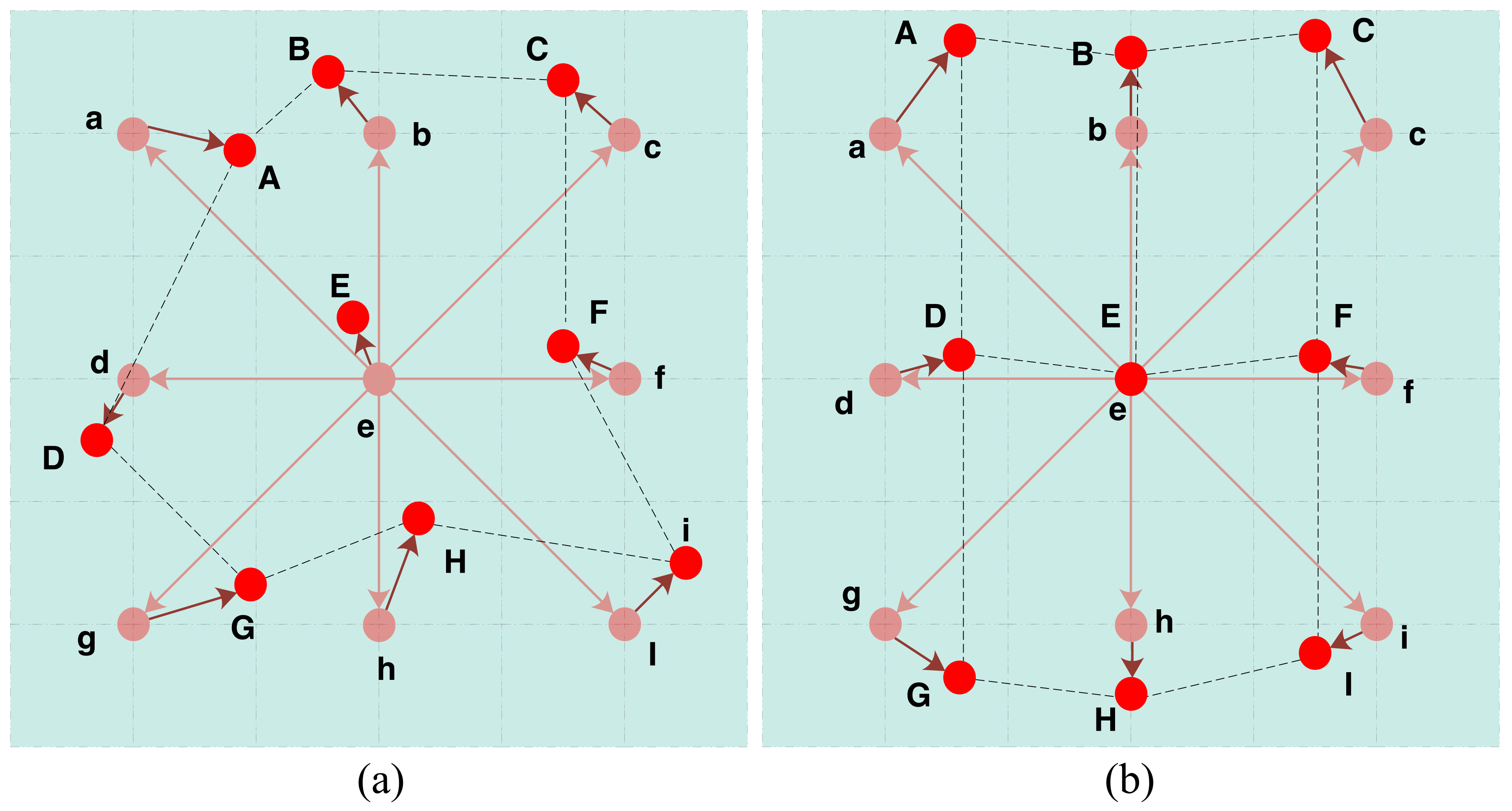
Figure 2: Illustrations of conventional DConv and our NDConv, as demonstrated in (a) and (b). The sampling points are represented by the balls. Among them, the pink balls represent the sampling points of the conventional convolution (indicated by lowercase letters, a-i), the red balls represent the actual sampling points (indicated by uppercase letters A-I), and the offsets are represented by the dark purple arrows.

$$\mathcal{L}_{A}=\|(d+\Delta D)+(b+\Delta B)-(e+\Delta E)-a\|_{2}^{2}$$ (4)

$$\mathcal{L}_{C}=\|(f+\Delta F)+(b+\Delta B)-(e+\Delta E)-c\|_{2}^{2}$$

$$\mathcal{L}_{G}=\|(d+\Delta D)+(h+\Delta H)-(e+\Delta E)-g\|_{2}^{2}$$

$$\mathcal{L}_{I}=\|(f+\Delta F)+(h+\Delta H)-(e+\Delta E)-i\|_{2}^{2}$$

Thus, NDloss can be presented as Eq.(5):

$$\mathcal{L}_{\text{nd}}=\mathcal{L}_{e}+\mathcal{L}_{\text{hor }}+\mathcal{L}_{\text{vec }}+\mathcal{L}_{A}+\mathcal{L}_{C}+\mathcal{L}_{G}+\mathcal{L}_{I}$$ (5)

Then, the loss of density estimation is:

$$\mathcal{L}_{den}=\min_{\Phi}\frac{1}{2N}\left\|P\left(I_{i};\boldsymbol{\Phi}\right)-Y_{i}\right\|_{2}^{2}$$ (6)

Y_i is the density map of ground_truth, $\boldsymbol{\Phi}$ denotes the parameters of the network, $P\left(I_{i};\boldsymbol{\Phi}\right)$ represents the estimation of density map, and $N$ is the batch size. The final loss is:

$$\mathcal{L}_{all}=\mathcal{L}_{den}+\lambda\mathcal{L}_{nd}$$ (7)

where $\lambda$ is the super-parameter to balance the two losses.

II-B Net Architecture

The architecture of the network is illustrated in Fig. 3. CSRNet[19] is adopted as the backbone network, specifically, we add Batch Normalziation

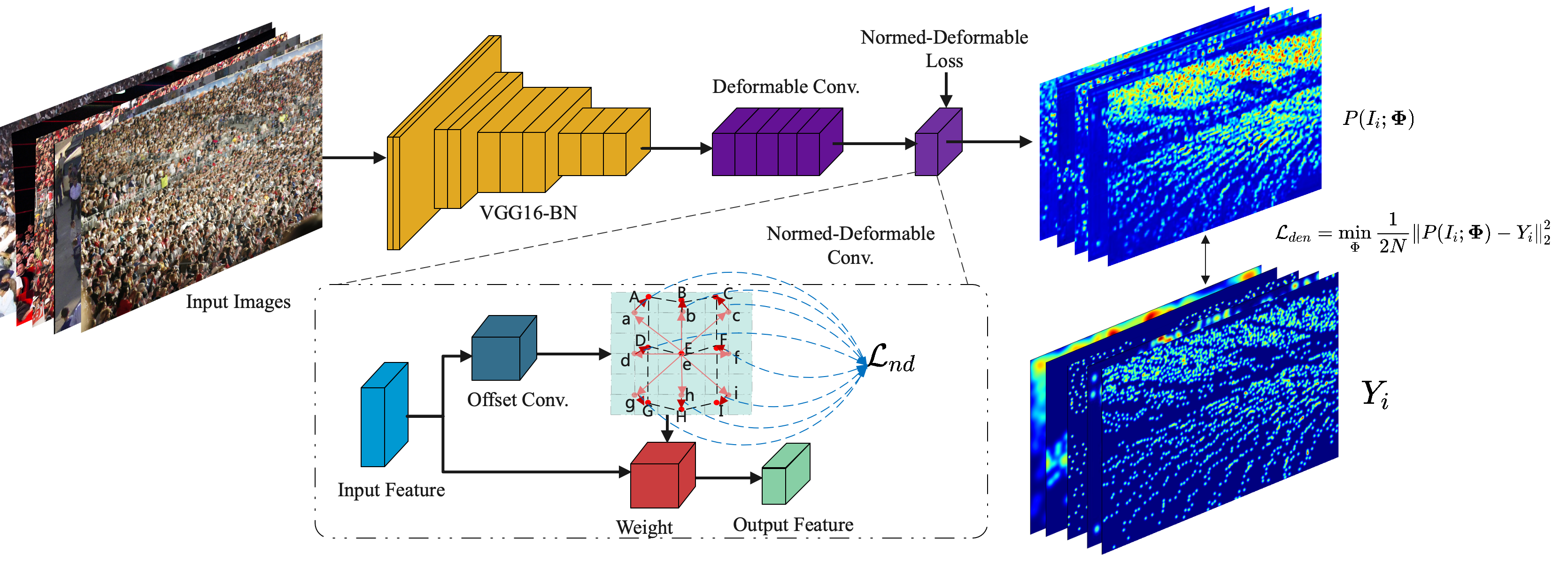
Figure 3: The architecture of the proposed NDConv network. We adopt CSRNet$\star$ as our backbone, where the last layer of dilated convolution is replaced with NDConv to constrain the sampling points.

layer after each convolution layer to enhance the robustness of training with cropped images. After that, the last layer of dilated convolution is replaced with DConv or NDConv, denoted as CSRNet$\star$ and CSRNet (NDConv), respectively. In the next section, the effectiveness of our NDConv is verified.

III Experimental results

In this section, four datasets are adopted in our experiments, including ShanghaiTech A, ShanghaiTech B[4], UCF-QRNF[20], and UCF_CC_50[21]. Firstly, the evaluation metric and datasets are introduced, and then the implementation details are described. Subsequently, the proposed NDconv is compared with state-of-the-art methods on the four above-mentioned datasets. Finally, the ablation study is conducted to explain the meaning of parameters in experiments.

III-A Datasets and Implementation Details

III-A1 Datasets

On four popular datasets, ShanghaiTech Part A, ShanghaiTech Part B, UCF-QNRF, and UCF_CC_50, the proposed NDConv and other state-of-the-art approaches are evaluated.

ShanghaiTech[4]. It is composed of part A and part B. For Part A, the images are obtained from the web, and the images in Part B are views of Shanghai streets. Part A contains $482$ crowd images. Different from Part A, there are more high-resolution images in Part B. It contains $716$ images, while the counts of crowd in per image is from $9$ to $578$.

UCF-QNRF[20]. Compared with ShanghaiTech, this is a larger crowd counting dataset that contains $1,535$ high-resolution images and $1.25$ million head annotations. In this dataset, there are $1,201$ images of extremely congested scenes for training and the rest are test images. The maximum count of an image is $12,865$.

UCF_CC_50[21]. In our experiment, there is also a challenging dataset called UCF_CC_50 which contains $50$ images. Although the number of images is small, the count in per image varies drastically from $94$ to $4,543$. Following the setting in [21], we divide the dataset into five subsets, and then $5$-fold cross-validation is performed.

III-A2 Evaluation Metric

Mean Absolute Error (MAE) and Mean Square Error (MSE) are adopted as the evaluation metrics, same as the previous works [22, 23, 24].

III-A3 Implementation Details

To improve the robustness of training with cropped images, the backbone of CSRNet[19] is replaced with VGG16-BN and we insert Batch-Normalization[42] layer after each dilated convolution. Then, the last layer of dilated convolution is replaced with DConv. After these changes, the model is termed as CSRNet$\star$ and is the baseline of experiments. Subsequently, the last layer of DConv is replaced with NDconv, denoted as Ours (NDConv).

In the experiments, we use a fixed $\!7\times\!7$ Gaussian kernel to generate density maps and Adam[25] optimizer is used with a learning rate of $1$e-$4$. All images are resized to $\!400\times\!400$. The batch size and parameter $\lambda$ are set to $4$ and $0.001$. We train $400$ epochs in two days.

III-B Evaluations and Comparisons

The results of experiments on ShanghaiTech A and B are shown in Table I.

TABLE I: Comparisons on Shanghaitech A and B

Methods	Venue&Year	ShanghaiTechA		ShanghaiTechB
		MAE	MSE	MAE	MSE
CSRNet[19]	CVPR2018	$68.2$	$115.0$	$10.6$	$16.0$
SANet[28]	CVPR2018	$67.0$	$104.5$	$8.4$	$13.6$
TEDnet[29]	CVPR2019	$64.2$	$109.1$	$8.2$	$12.8$
ADCrowdNet[24]	CVPR2019	$63.2$	$98.9$	$8.2$	$15.7$
PSDDN[30]	CVPR2019	$65.9$	$112.3$	$9.1$	$14.2$
HA-CNN[26]	TIP2019	$62.9$	94.9	$8.1$	$13.4$
LSC-CNN[27]	TPAMI2020	$66.4$	$117.0$	$8.1$	12.7
DensityCNN[31]	TMM2020	$63.1$	$106.3$	$9.1$	$16.3$
DENet[32]	TMM2020	$65.5$	$101.2$	$9.6$	$15.4$
CSRNet$\star$(Baseline)	-	$65.0$	$102.63$	$9.0$	$15.3$
Ours(NDConv)	-	61.4	$104.18$	7.8	$13.8$

Compared with state-of-the-art, our method performs the best, indicating the advantages of constrained offsets in deform convolution. For ShanghaiTech A, our method achieves the best $61.4$ MAE with $2.5$ performance improvement against the baseline CSRNet$\star$. The result of evaluation on ShanghaiTech B has also lived up to expectations, our method achieves $7.8$ MAE and $13.3$ relative MAE decrease with the baseline.

TABLE II: Comparisons on UCF-QNRF and UCF_CC_50

Methods	Venue&Year	UCF-QNRF		UCF_CC_50
		MAE	MSE	MAE	MSE
CSRNet[19]	CVPR2018	-	-	$266.1$	$397.5$
SANet[28]	CVPR2018	-	-	$258.4$	$334.9$
TEDnet[29]	CVPR2019	$113$	$188$	$294.4$	$354.5$
ADCrowdNet[24]	CVPR2019	-	-	$257.1$	$363.5$
PSDDN[30]	CVPR2019	-	-	$359.4$	$514.8$
HA-CCN[26]	TIP2019	$118.1$	$180.4$	$256.2$	$348.4$
LSC-CNN[27]	TPAMI2020	$120.5$	$218.2$	$225.6$	$302.7$
DensityCNN[31]	TMM2020	$101.5$	$186.9$	$244.6$	$341.8$
DENet[32]	TMM2020	-	-	$241.9$	$345.4$
DS-CNN[43]	AJSE2021	$115.2$	$175.7$	$229.4$	$325.6$
SDIH-DDM[44]	TVCJ2020	$112$	$173$	-	-
CSRNet$\star$(Baseline)	-	$95.5$	165.3	$174.6$	237.0
Ours(NDConv)	-	91.2	$165.6$	167.2	$240.6$

For the datasets, UCF-QNRF and UCF_ CC_50, the comparison between our methods and state-of-the-arts is recorded in Table II. Compared with the baseline CSRNet$\star$, our method achieves significant gain on MAE. Respectively, $91.2$ and $167.2$ MAE are achieved on datasets UCF-QNRF and UCF_CC_50, with $4.5$%, $4.2$% performance improving. In particular, on the premise of great performance improvement on CSRNet$\star$, our method further reduces MAE, indicating the effectiveness of the constrained offsets in the dense scene.

III-C Ablation Study

In this section, the influence of the number of deformable layers in our network is demonstrated firstly. On the other hand, visualization of the constrained offsets is shown in Fig. 4  and the validity of NDloss is verified. Finally, the extensibility of NDConv on another backbone is indicated.

III-C1 Influence of the number of deformable layers

There are $6$ layers of dilated convolution integrated into the architecture of CSRNet. Each layer of dilated convolution is changed into Deformable Convolution gradually. Then, each layer of Deformable Convolution is replaced with NDConv. The performance is shown in Table III. While the number of deformable layers is increased, the performance of the above-mentioned experiment is decreased. The peak values of baseline are from $172.9$ to $187.4$ MAE, while the trend in performance of NDConv is similar, which is from $167.2$ to $184.6$ MAE on UCF_CC_50. Thus, the effectiveness is better by only replacing the last layer of dilated convolution with DConv and NDConv respectively in the network.

TABLE III: Effects of the number of deformable layers on UCF_CC_50

Deformable Layers	CSRNet$\star$		Ours(NDConv)
	MAE	MSE	MAE	MSE
1	$174.6$	$237.0$	167.2	$240.6$
2	172.9	$268.3$	$185.0$	$296.1$
3	$175.4$	233.3	$168.2$	235.4
4	$182.7$	$271.2$	$177.2$	$245.9$
5	$187.4$	$266.5$	$177.6$	$235.7$
6	$174.9$	$256.2$	$184.6$	$263.3$

III-C2 Visualization of offsets

Experiments have shown that our NDConv surpasses Deformable Convolution and the visualization of the offsets in Fig. 4 as previous work[34] also validates our hypothesis. Fig. 4(c) and Fig. 4(f) demonstrate the sampling points of DConv and our proposed NDConv. It is obvious that the sampling points of NDConv tend to be spread more uniformly over the heads, leading to more sufficient feature aggregation. Accordingly, Fig. 4(e) shows more regular Gaussian blobs than Fig. 4(d), which further verifies the reasonableness of our NDConv.

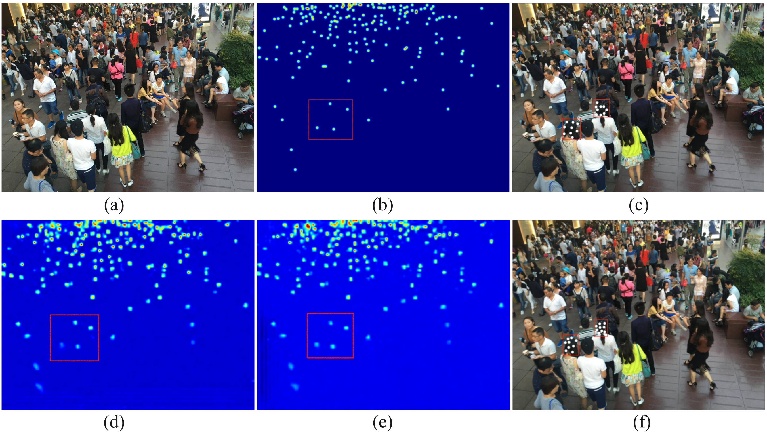
Figure 4: Visualization of an example from ShanghaiTech B dataset. (a) is the input image; (b) is the ground_truth; (c) and (f) are the visualization of offsets in DConv and NDConv; the predicted density map in DConv and NDConv are shown in (d) and (e).

III-C3 Extensibility to Another Backbone

A new baseline consisted of ResNet-50[33] is built to verify the extensibility of NDConv. Firstly, ResNet-50 (backbone) with the four dilated convolutions is not changed. Then, the last layer of dilated convolutions is replaced with Deformable Convolution as the new baseline called ResNet-50 (DConv). Finally, the layer of Deformable Convolution is replaced with NDConv in ResNet-50 (NDConv). The comparisons of results on UCF_QNRF and UCF_CC_50 are shown in Table IV. For ResNet-50 (backbone), we get $99.3$ and $227.6$ MAE on UCF_QNRF and UCF_CC_50, respectively. When the last layer of convolution is replaced with Deformable Convolution, the baseline delivers $98.0$ and $231.3$ MAE. Particularly, if the layer of Deformable Convolution is replaced by NDConv, a better performance is achieved $95.4$ and $222.4$ MAE. The extensibility and effectiveness of NDConv on another backbone are indicated by the results of the experiment.

TABLE IV: Comparisons on the ResNet-50 backbone

Methods	UCF_QNRF		UCF_CC_50
	MAE	MSE	MAE	MSE
ResNet-50(backbone)	$99.3$	$181.5$	$227.6$	307.6
ResNet-50(DConv)	$98.0$	178.0	$231.3$	$317.0$
ResNet-50(NDConv)	95.9	$182.4$	222.4	$315.4$

III-C4 The effects of $\mathcal{L}_{nd}$

The final loss consists of $\mathcal{L}_{nd}$ and $\mathcal{L}_{den}$. In this section, the effect of super-parameter $\lambda$ is investigated. The performance varies with the values of $\mathcal{L}_{nd}$. By conducting the ablation study, it is verified that when the weight of the super-parameter $\lambda$ is $1$e-$3$, the better performance is achieved. The experimental data is shown in Table V.

TABLE V: Effects of the weight of $\mathcal{L}_{nd}$ on UCF-QNRF and UCF_CC_50

Datasets	Metrics	$\lambda$(super-parameter)
		$1$e-$1$	$1$e-$2$	$1$e-$3$	$1$e-$4$	$0$
UCF-QNRF[20]	MAE	$94.8$	$95.6$	91.2	$93.8$	$95.5$
	MSE	$167.4$	165.2	$165.6$	$167.2$	$165.3$
UCF_CC_50[21]	MAE	$189.5$	$182.4$	167.2	$175.2$	$174.6$
	MSE	$264.2$	$285.1$	$240.6$	$238.7$	237.0

IV Conclusion

Normed-Deformable Convolution(NDConv) is proposed in this paper, which shows its specificity in the constrained sampling offsets via NDloss. NDloss is designed under the guidance of the shape of head, so as to enhance the effectiveness of feature aggregation. Experiments show that our proposed NDConv surpasses the conventional Deformable Convolution over four popular datasets with little extra computational burden.

References

- [1] Q. Wang, J. Gao, and W. Lin, “NWPU-Crowd: A Large-Scale Benchmark for Crowd Counting and Localization,” in IEEE Transactions on Pattern Analysis and Machine Intelligence, 2020: 3013269.
- [2] P. L. Mazzeo, R. Contino, and P. Spagnolo, “MH-MetroNet-A Multi-Head CNN for Passenger-Crowd Attendance Estimation,” in Journal of Imaging, vol. 6, no. 7, pp. 62, 2020.
- [3] V. A. Sindagi and V. M. Patel, “Generating high-quality crowd density maps using contextual pyramid cnns,” in Proceedings of the IEEE International Conference on Computer Vision(ICCV), pp. 1879-1888, 2017.
- [4] Y. Zhang, D. Zhou, S. Chen, S. Gao, and Y. Ma, “Single-image crowd counting via multi-column convolutional neural network,” in Proceedings of the IEEE Conference on Computer Vision and Pattern Recognition(CVPR), pp. 589-597, 2016.
- [5] R. S. Feris, B. Siddiquie, and J. Petterson, “Large-Scale Vehicle Detection, Indexing, and Search in Urban Surveillance Videos,” in IEEE Transactions on Multimedia, vol. 14, no. 1, pp. 28-42, 2012.
- [6] G. Wang, B. Li, Y. Zhang, and J. Yang, “Background modeling and referencing for moving cameras-captured surveillance video coding in hevc,” in IEEE Transactions on Multimedia, vol. 20, no. 11, pp. 2921-2934, 2018.
- [7] E. Ran and Y. Moses, “Tracking in a Dense Crowd Using Multiple Cameras,” in International Journal of Computer Vision, vol. 88, no. 1, pp. 129-143, 2010.
- [8] G. J. Brostow and R. Cipolla, “Unsupervised bayesian detection of independent motion in crowds,” in Proceedings of the IEEE Conference on Computer Vision and Pattern Recognition(CVPR), vol. 1, pp. 594-601, 2006.
- [9] V. Rabaud and S. Belongie, “Counting crowded moving objects,” in Proceedings of the IEEE Conference on Computer Vision and Pattern Recognition(CVPR), vol. 1, pp. 705-711, 2006.
- [10] A. B. Chan and N. Vasconcelos, “Bayesian poisson regression for crowd counting,” in IEEE International Conference on Computer Vision(ICCV), pp. 545-551, 2010.
- [11] K. Chen, C. C. Loy, S. G. Gong, and T. Xiang, “Feature mining for localised crowd counting,” in British Machine Vision Conference(BMVC), vol. 1, p. 3, 2012.
- [12] M. S. Zitouni, H. Bhaskar, J. Dias, and M. E. AlMualla, “Advances and trends in visual crowd analysis: A systematic survey and evaluation of crowd modelling techniques,” in Neurocomputing, vol. 186, pp. 139-159, 2016.
- [13] V. A. Sindagi and V. M. Patel, “A survey of recent advances in cnn-based single image crowd counting and density estimation,” in Pattern Recognition Letters, vol. 107, pp. 3-16, 2017.
- [14] C. Shang, H. Ai, and B. Bai, “End-to-end crowd counting via joint learning local and global count,” in IEEE International Conference on Image Processing(ICIP), pp. 1215-1219, 2016.
- [15] F. Yu and V. Koltun, “Multi-scale context aggregation by dilated convolutions,” in International Conference on Learning Representations(ICLR), 2016: 9321067.
- [16] D. B. Sam, S. Surya, and R. V. Babu, “Switching convolutional neural network for crowd counting,” in Proceedings of the IEEE Conference on Computer Vision and Pattern Recognition(CVPR), pp. 4031-4039, 2017.
- [17] J. Dai, H. Qi, and Y. Xiong, “Deformable Convolutional Networks,” in Proceedings of the IEEE International Conference on Computer Vision(ICCV), pp. 764-773, 2017.
- [18] X. Zhu, H. Hu, and S. Lin, “Deformable ConvNets V2: More Deformable, Better Results,” in Proceedings of the IEEE Conference on Computer Vision and Pattern Recognition(CVPR), 2019: 00953.
- [19] Y. Li, X. Zhang, and D. Chen, “CSRNet: Dilated Convolutional Neural Networks for Understanding the Highly Congested Scenes,” in Proceedings of the IEEE Conference on Computer Vision and Pattern Recognition(CVPR), 2018: 00120.
- [20] H. Idrees, M. Tayyab, K. Athrey, D. Zhang, S. AlMaadeed, N. Rajpoot, and M. Shah, “Composition loss for counting, density map estimation and localization in dense crowds,” in Lecture Notes in Computer Science , pp. 532-546, 2018.
- [21] H. Idrees, I. Saleemi, C. Seibert, and M. Shah, “Multi-source multi- scale counting in extremely dense crowd images,” in Proceedings of the IEEE Conference on Computer Vision and Pattern Recognition(CVPR), pp. 2547-2554, 2013.
- [22] Y. Yang, G. Li, and D. Du, “Embedding Perspective Analysis Into Multi-Column Convolutional Neural Network for Crowd Counting,” in IEEE Transactions on Image Processing, no. 30, pp. 1395-1407, 2021.
- [23] Z. Yan, Y. Yuan, and W. Zuo, “Perspective-Guided Convolution Networks for Crowd Counting,” in Proceedings of the IEEE International Conference on Computer Vision(ICCV), 2019: 00104.
- [24] N. Liu, Y. Long, and C. Zou, “ADCrowdNet: An Attention-Injective Deformable Convolutional Network for Crowd Understanding,” in Proceedings of the IEEE Conference on Computer Vision and Pattern Recognition(CVPR), pp. 3220-3229, 2019.
- [25] D. Kingma and J. Ba, “Adam: A Method for Stochastic Optimization,” in Computer Science, pp. 273-297, 2014.
- [26] V. A. Sindagi and V. M. Patel, “Ha-ccn: Hierarchical attention-based crowd counting network,” in IEEE Transactions on Image Processing, vol. 29, pp. 323-335, 2019.
- [27] D. B. Sam, S. V. Peri, M. N. Sundararaman, A. Kamath, and V. B. Radhakrishnan, “Locate, size and count: Accurately resolving people in dense crowds via detection,” in IEEE Transactions on Pattern Analysis and Machine Intelligence, vol. 43, no. 8, pp. 2739-2751, 2021.
- [28] X. Cao, Z. Wang, Y. Zhao, and F. Su, “Scale aggregation network for accurate and efficient crowd counting,” in Lecture Notes in Computer Science, pp. 734-750, 2018.
- [29] X. Jiang, Z. Xiao, B. Zhang, X. Zhen, X. Cao, D. Doermann, and L. Shao, “Crowd counting and density estimation by trellis encoder- decoder networks,” in Proceedings of the IEEE Conference on Computer Vision and Pattern Recognition(CVPR), pp. 6133-6142, 2019.
- [30] Y. Liu, M. Shi, Q. Zhao, and X. Wang, “Point in, box out: Beyond counting persons in crowds,” in Proceedings of the IEEE Conference on Computer Vision and Pattern Recognition(CVPR), pp. 6469-6478, 2019.
- [31] X. Jiang, L. Zhang, T. Zhang, P. Lv, B. Zhou, Y. Pang, M. Xu, and C. Xu, “Density-aware multi-task learning for crowd counting,” in IEEE Transactions on Multimedia, 2020: 2980945.
- [32] L. Liu, W. Jia, J. Jiang, S. Amirgholipour, Y. Wang, M. Zeibots, and X. He, “Denet: A universal network for counting crowd with varying densities and scales,” in IEEE Transactions on Multimedia, 2020: 2992979.
- [33] K. He, X. Zhang, and S. Ren, “Deep Residual Learning for Image Recognition,” in Proceedings of the IEEE Conference on Computer Vision and Pattern Recognition(CVPR), pp. 770-778, 2016.
- [34] Z. Yan, R. Zhang, H. Zhang, Q. Zhang, and W. Zuo. “Crowd Counting via Perspective-Guided Fractional-Dilation Convolution,” in IEEE Transactions on Multimedia, 2021: 3086709.
- [35] Q. Song, C. Wang, Y. Wang, Y. Tai, C. Wang, and J. Li, “To Choose or to Fuse Scale Selection for Crowd Counting,” in Proceedings of the AAAI Conference on Artificial Intelligence, vol.35, pp. 2576-2583, 2021.
- [36] J. Wan, “A Generalized Loss Function for Crowd Counting and Localization,” in Proceedings of the IEEE Conference on Computer Vision and Pattern Recognition(CVPR), pp. 1974-1983, 2021.
- [37] B. Yang, W. Zhan, N. Wang, X. Liu, and J. Lv, “Counting crowds using a scale-distribution-aware network and adaptive human-shaped kernel,” in Neurocomputing, vol. 390, pp. 207-216, 2020.
- [38] Y. Fang, B. Zhan, W. Cai, S. Gao, and B. Hu, “Locality-constrained spatial transformer network for video crowd counting,” in Proceedings IEEE International Conference on Multimedia and Expo(ICME), vol. 2019-July, pp. 814-819, 2019.
- [39] F. Xiong, X. Shi, and D. Yeung, “Spatiotemporal Modeling for Crowd Counting in Videos,” in Proceedings of the IEEE International Conference on Computer Vision(ICCV), vol. 2017-October, pp. 5161-5169, 2017.
- [40] Y. Ma, H. Shuai, and W. Cheng, “Spatiotemporal Dilated Convolution with Uncertain Matching for Video-based Crowd Estimation,” in IEEE Transactions on Multimedia, 2021: 3050059.
- [41] Y. Fang, S. Gao, J. Li, W. Luo, L. He, and B. Hu, “Multi-level feature fusion based Locality-Constrained Spatial Transformer network for video crowd counting,” in Neurocomputing, vol. 392, pp. 98-107, 2020.
- [42] S. Ioffe and C. Szegedy, “Batch normalization: Accelerating deep network training by reducing internal covariate shift,” in 32nd International Conference on Machine Learning(ICML), vol. 1, pp. 448-456, 2015.
- [43] S. D. Khan, and S. Basalamah, “Sparse to Dense Scale Prediction for Crowd Counting in High Density Crowds,” in Arabian Journal for Science and Engineering, vol. 46, no. 4, pp. 3051-3065, 2021.
- [44] S. D. Khan, and S. Basalamah, “Scale and density invariant head detection deep model for crowd counting in pedestrian crowds,” in The Visual Computer, vol. 37, no. 8, pp. 2127-2137, 2020.