Unsteady ballistic heat transport in a 1D harmonic crystal due to a source on an isotopic defect

Abstract

In the paper we apply asymptotic technique based on the method of stationary phase and obtain the approximate analytical description of thermal motions caused by a source on an isotopic defect of an arbitrary mass in a 1D harmonic crystal. It is well known that localized oscillation is possible in this system in the case of a light defect. We consider the unsteady heat propagation and obtain formulae, which provide continualization (everywhere excepting a neighbourhood of a defect) and asymptotic uncoupling of the thermal motion into the sum of the slow and fast components. The slow motion is related with ballistic heat transport, whereas the fast motion is energy oscillation related with transformation of the kinetic energy into the potential one and in the opposite direction. To obtain the propagating component of the fast and slow motions we estimate the exact solution in the integral form at a moving point of observation. We demonstrate that the propagating parts of the slow and the fast motions are “anti-localized” near the defect. The physical meaning of the anti-localization is a tendency for the unsteady propagating wave-field to avoid a neighbourhood of a defect. The effect of anti-localization increases with the absolute value of the difference between the alternated mass and the mass of a regular particle, and, therefore, more energy concentrates just behind the leading wave-front of the propagating component. The obtained solution is valid in a wide range of a spatial co-ordinate (i.e., a particle number), everywhere excepting a neighbourhood of the leading wave-front.

1 Introduction

A one-dimensional harmonic crystal (a uniform chain of particles connected by linear springs) is a rather old classical mechanical model. Hamilton seems to be the first who investigated the dynamics of a uniform chain Hamilton1940 . Later this problem was rediscovered by Havelock Havelock1910 and Schrödinger schrodinger1914dynamik ; Muehlich2020 . Schrödinger obtained the general solution for the dynamical problem and suggested applying this model to investigate heat transfer in crystals. The idea was realized by many researchers, among the first works we underline the studies by Klein & Prigogine klein1953mecanique , Hemmer hemmer1959dynamic , Rieder, Lebowitz, and Lieb rieder1967properties . It was shown rieder1967properties ; lepri2003thermal that heat transport in harmonic crystals violates the Fourier low. Nowadays, this regime of heat propagation is known as the ballistic one, and it is experimentally observed in ultra-pure low-dimensional nano-materials chang2008breakdown ; hsiao2015micron ; hsiao2013observation under certain conditions, in particular, in graphene Bae2013 ; Saito2018 ; Xu2014 . These new applications increased again the interest to the model of a harmonic crystal. Krivtsov, Kuzkin and their colleagues who considered the heat propagation in harmonic crystals suggested separating the slow and the fast thermal processes krivtsov2014energy ; krivtsov2015heat ; Kuzkin-Krivtsov-accepted ; krivtsov-da70 , and formulated the simplified continuum equations involving only the slow motion. The slow motion is related with heat transport krivtsov2015heat ; Gavrilov2019cmat , whereas the fast motion is energy oscillation related with transformation of the kinetic energy into the potential one and in the opposite direction klein1953mecanique ; krivtsov2014energy ; Gavrilov2019PhysRevE ; kuzkin2019thermal . A comparison of the continuum approach by Krivtsov with discrete approach by Hemmer is given in Sokolov2021 . In this way, a general technique was suggested that allows one to derive the simplified continuum equation for the slow motion and analytically investigate the unsteady and steady-state heat transport in uniform harmonic crystals of general kind, e.g., polyatomic lattices Kuzkin2019 . This technique was applied, in particular, to a graphene lattice Kuzkin2019 ; Gavrilov2022cmat ; Panchenko2022 . It, nevertheless, is not directly applicable to spatially non-uniform systems. Recently Gavrilov Gavrilov2022ijhmt noticed that the expression for the slow motion in a 1D uniform chain can be formally obtained as the slow time-varying component of the large-time asymptotics for the exact discrete solution at a moving point of observation. The approach involving a moving point of observation, which is known to us due to Slepyan1972 in context of continuum problems, allows one to describe running waves, wave-fronts, and the wave-field as a whole, in comparison with the evaluation of the corresponding asymptotics at a fixed position. The last approach can be easily generalized to spatially non-uniform systems.

One of the first studies concerning a 1D chain with a single isotopic defect is Montroll1955 , where a spectral problem is considered, and it is proved that a localized mode exists in such a system in the case of a light defect. A localized (or trapped) mode is a general phenomenon, which can be observed in discrete and continuum systems. The extensive bibliography on localized modes in discrete and continuum mechanical systems can be found in Ind-book-R2E ; Andrianov2012 ; Gavrilov2019nody ; Mishuris2020 . Teramoto & Takeno Teramoto1960 were probably the first who treated a localized oscillation in the chain with the defect as a non-stationary non-vanishing motion in time. Kashiwamura Kashiwamura1962 obtained a rough estimation for the particle velocity of an initially perturbed heavy defect as $O(t^{-3/2})$, whereas in a uniform chain the corresponding asymptotics is $O(t^{-1/2})$, $t\to\infty$ is the time. Hemmer hemmer1959dynamic , Magalinskii magalinskii1959dynamical , Müller Mueller1962 (see also Mueller2012 ) considered the particular case of a very heavy isotope defect. Turner Turner1960 obtained the solution (the momentum autocorrelation function) describing the motion for the defect in the case of a source on a heavy defect as a series with terms involving Bessel functions. For the defect of the double mass this solution becomes a lot simpler. Rubin published a series of studies Rubin1960 ; Rubin1961 ; Rubin_1963 . In Rubin1960 ; Rubin1961 the general problem statement for a cubic lattice was discussed and some particular results for a 1D chain were obtained. One-dimensional case was discussed in detail in Rubin_1963 . It was demonstrated that together with the localized component, which exists only for a light defect, the solution (the momentum autocorrelation function) always contains a vanishing propagating component. This component, which is $O(t^{-3/2})$ at the defect (as was obtained by Kashiwamura Kashiwamura1962 for the case of a heavy defect), was calculated in the explicit form for any defect mass. Outside the defect some particular limiting results were obtained for the case of the defect of the double mass (in a zone behind the leading wave-front). In the latter case the obtained result coincides with the corresponding result for the uniform chain (see Remark 7). Also, the transport of energy was considered and the ratio of the energy trapped by the localized mode was calculated. Takizawa & Kobayasi Takizawa1967 ; Takizawa1968 obtained the general solution for the problem concerning a chain with an isotope defect of an arbitrary mass as a series with terms involving Bessel functions. This solution has enough complicated form and is difficult for analysis.

In Lee1989 the dynamics of a harmonic chain with an isotopic defect is considered basing on the recurrence relations method. This method allows one to consider also diatomic chains with an isotopic defect Yu2014 ; Yu2015 ; Yu2016 . In Yu2019 a chain with an impurity in mass and Hooke constant is considered by the recurrence relations. In all these studies the solution is obtained only for the defect particle.

In several studies kannan2013heat ; Paul2020 ; Gendelman2021 ; Plyukhin2020 the classical steady-state formulation of the problem concerning thermal conductivity of a finite chain with an isotopic defect is considered. Gendelman & Paul Paul2020 ; Gendelman2021 suggested using this model to describe the Kapitza thermal resistance. Plyukhin Plyukhin2020 indicated that in the framework of the model non-Clausius heat transfer (from cold to hot) is possible. Experimental studies (e.g., Chen2012 ) demonstrate that the presence of isotopic defects essentially influences on the thermal conductivity of a pure graphene. Phonon scattering by an isotope defect in graphene is considered in Saito2018 .

In this paper we apply the asymptotic technique based on the method of stationary phase to an integral representation for the solution and obtain the approximate analytical description of the thermal motion caused by a source on an isotopic defect in a 1D harmonic crystal. We re-obtain some necessary known results, mostly related with localized oscillation and asymptotics of the solution just on a defect, to get necessary intermediate formulae and make the analysis more complete.

The new results of the paper are related mostly with the propagating component of the motion. These results have been obtained due to a mathematical approach, which is well-known for continuum systems Slepyan1972 , but, as far as we know, seems to be quite new Gavrilov2022ijhmt for discrete systems. Following to Gavrilov2022ijhmt , we estimate the exact solution in the integral form at a moving point of observation. For a discrete system, the new approach directly provides continualization and slow-and-fast motions decoupling, as well as a possiblity to obtain the approximate solution in a wide range of a spatial co-ordinate (i.e., a particle number), whereas the previous solutions describe only the isotopic defect motion and leading wave-fronts. The obtained solution has a simple structure and is valid for any value of the defect mass, although it, as well as all previous solutions, are not applicable in a neighbourhood of the defect with the mass close to the mass of a regular particle. It demonstrates us that the propagating parts of the slow and the fast motions are “anti-localized” near the defect. The physical meaning of the anti-localization is a tendency for the unsteady propagating wave-field to avoid a neighbourhood of a defect. The effect of anti-localization increases with the absolute value of the difference between the alternated mass and the mass of a regular particle, and, therefore, more energy concentrates just behind the leading wave-front of the propagating component. For the best of our knowledge, this important qualitative finding is also new. The separation of slow motions allows one to essentially simplify krivtsov2015heat ; Kuzkin-Krivtsov-accepted ; krivtsov-da70 ; Gavrilov2019cmat ; Sokolov2021 ; Kuzkin2019 ; Gavrilov2022cmat the description of the ballistic heat transfer and gives the possibility to consider complicated systems, in particular, 2D–3D polyatomic lattices. Therefore, we expect that our approach can also be applied to such a system with defects.

Thus, two ideas that allow us to obtain the more complete and simple description of ballistic heat transfer in the system under consideration are

• Separation of slow motions, suggested in krivtsov2015heat ;

• Estimation of the exact solution in the integral form at a continuously moving point of observation, suggested for a discrete system in Gavrilov2022ijhmt .

It is important that both of the ideas are applicable for more complicated lattices with defects.

The paper is organized as follows. In Sect. 2 we introduce general notation. In Sect. 3 we discuss the mathematical formulation. In Sect. 3.1 we introduce an auxiliary deterministic problem for the chain with an isotopic defect, and the corresponding fundamental solution describing the particle velocity. The momentum autocorrelation function, which is traditionally used to describe the motion in the system, equals this fundamental solution with accuracy to a constant multiplier. In Sect. 3.2 we formulate the thermal (random) problem and introduce the corresponding fundamental solution, describing the propagation of the kinetic temperature along the chain. This thermal fundamental solution can be expressed in terms of the squared fundamental solution describing the particle velocity. In Sect. 4 we discuss the dispersion relation and its properties in the pass-band and the stop-band. In Sect. 5 we introduce the Green function in the frequency domain for the pass-band and the stop-band. In Sect. 6 we consider the spectral problem for the localized mode and get the formula for the frequency of localized oscillation. The material in Sects. 4–6 is definitely not new. In Sect. 7 we get the integral representation for the fundamental solution of the non-stationary deterministic problem for the particle velocity and proceed with asymptotic evaluation. In Sect. 7.1 we calculate the contribution from the pass-band (the propagating vanishing component) using the stationary phase method applied on a moving point of observation. These results are new. In Sect. 7.2 we calculate the contribution from the stop-band (a localized oscillation). The final results of Sect. 7.2 are not new, though we use the mathematical technique a bit different from the traditional one. Namely, we prefer to use asymptotic integration over the real line, using the theory of Fourier transform for generalized functions (or distributions), the limit absorption principle and the Sokhotski–Plemelj theorem for the real line, instead of Laplace transform and integration over a contour in the complex plane. In Sect. 7.3 we calculate the contribution from the cut-off frequency and re-obtain the asymptotics for the particle velocity of the defect got by Rubin Rubin_1963 . In Sect. 7.4 we calculate the corresponding asymptotics on the leading wave-front. In Sect. 7.5 we discuss the asymptotics before the leading wave-fronts, this result seems to be new. To make the results reproducible, we present detailed calculations for all asymptotics. For a reader who prefers to skip the details, it is possible to find the most important formulae summarized in Sect. 7.6. In Sect. 8 we compare the obtained results with numerical ones and demonstrate a good agreement. In Sect. 9 we discuss the domain of applicability for our results and compare them with ones previously obtained in Rubin_1963 . In Sect. 10 we return to the thermal problem and obtain formulae, which provide continualization and asymptotic uncoupling of the thermal motion into the sum of the slow and fast components. In Sect. 11 we discuss the basic results of the paper and their possible generalizations. In Appendix A we derive non-dimensional formulation, which is used everywhere in the paper. In Appendix B we provide the formulation of the Erdélyi lemma, which is used to calculate the asymptotics. In Appendix C we calculate the trapped energy ratio. This result is previously obtained in Rubin_1963 , but seems to be very important for understanding.

2 Nomenclature

In the paper, we use the following general notation:

$\mathbb{Z}$

is the set of all integers;

$\mathbb{R}$

is the set of all real numbers;

$C^{\infty}$

is the set of all infinitely differentiable functions;

$C_{0}^{\infty}$

is the set of all finite infinitely differentiable functions;

$H(\cdot)$

is the Heaviside function;

$\langle\cdot\rangle$

is the mathematical expectation for a random quantity;

$\delta_{n}$

is the Kronecker delta ($1$ if only if $n=0$, $0$ otherwise, $n\in\mathbb{Z}$);

$\delta(\cdot)$

is the Dirac delta-function;

$k_{B}$

is the (dimensionless) Boltzmann constant;

$J_{n}(\cdot)$

is the Bessel function of the first kind of order $n$;

$\Gamma(\cdot)$

is the Gamma function;

$\operatorname{PV}$

is the Cauchy principal value for an integral;

$\mathrm{c.c.}$

are the complex conjugate terms;

$m$

is the dimensionless mass of an isotopic defect.

3 The problem formulation

3.1 The deterministic problem

Consider a chain of mass points of an equal mass with one alternated mass. All masses are connected by linear springs with the same stiffness. The equations of motions in the dimensionless form can be expressed as the following infinite system of differential-difference equations:

$$m_{n}\ddot{u}_{n}-(u_{n+1}-2u_{n}+u_{n-1})=\delta_{n}p(t).$$ (3.1)

Here $n\in\mathbb{Z}$, $u_{n}(t)$ is the dimensionless displacement of the particle with a number $n$, $m_{n}$ is the dimensionless mass of the particle with number $n$:

$$m_{n}=1+\delta_{n}(m-1),$$ (3.2)

overdot denotes the derivative with respect to the dimensionless time $t$. We assume that the dimensionless mass of the defect particle $m=m_{0}$ is such that

$$m>0,\qquad m\neq 1.$$ (3.3)

The dimensionless external force $p(t)$ is applied to the zeroth particle with alternated mass. Equation (3.1) can be transformed to the following equivalent form:

$$\ddot{u}_{n}-(u_{n+1}-2u_{n}+u_{n-1})=\delta_{n}P(t),$$ (3.4)

$$P(t)=-(m-1)\ddot{u}_{0}+p(t),$$ (3.5)

where $P(t)$ is an unknown function. The differential-difference operator in the left-hand side of Eq. (3.4) corresponds to a uniform chain of mass points of unit mass connected by springs of unit stiffness.

Remark 1

In the paper we use the dimensionless problem formulation from the very beginning. Non-dimensionalization is discussed in Appendix A.

Since we are interested mostly in thermal processes, which are related with the propagation of the kinetic energy (or kinetic temperature), in what follows, we deal with the expression for the particle velocity $\dot{u}_{n}$. In the paper we use the fundamental solution

$$u_{n}={\mathcal{U}}_{n},\qquad\dot{u}_{n}={\mathcal{V}}_{n}\stackrel{{\scriptstyle\mbox{\scriptsize def}}}{{=}}\dot{\mathcal{U}}_{n}$$ (3.6)

of the deterministic problem, which corresponds to the choice of the external force as the pulse force

$$p(t)=\delta(t).$$ (3.7)

In this case the initial conditions for Eq. (3.1) can be formulated in the following form, which is conventional for distributions (or generalized functions) Vladimirov1971 :

$$u_{n}\big{|}_{t<0}\equiv 0.$$ (3.8)

The generalized initial value problem (3.1) with the right-hand side defined by Eq. (3.7) and initial conditions Eq. (3.8) can be equivalently formulated in the form of classical initial value problem for the system of equations

$$\begin{gathered}m_{n}\dot{{\mathcal{V}}}_{n}-({\mathcal{U}}_{n+1}-2{\mathcal{U}}_{n}+{\mathcal{U}}_{n-1})=0,\\ \dot{\mathcal{U}}_{n}={\mathcal{V}}_{n}\end{gathered}$$ (3.9)

with initial conditions in the classical form Vladimirov1971

$${\mathcal{U}}_{n}(0)=0,\qquad{\mathcal{V}}_{n}(0)=m_{n}^{-1}\delta_{n}\equiv m^{-1}\delta_{n}.$$ (3.10)

In the particular case $m=1$ of a uniform chain the exact expression for the fundamental solution ${\mathcal{V}}_{n}$ is schrodinger1914dynamik

$${\mathcal{V}}_{n}=J_{2n}(2t).$$ (3.11)

3.2 The random (thermal) problem

Consider the case of a point random initial excitation. Let the initial conditions for Eq. (3.9) be as follows:

$$u_{n}(0)=0,\qquad\dot{u}_{n}(0)=\rho{\delta_{n}}.$$ (3.12)

Here $n\in\mathbb{Z}$, $\rho$ is a random quantity such that

$$\langle\rho\rangle=0,\qquad\langle\rho^{2}\rangle=\sigma.$$ (3.13)

The (dimensionless) kinetic temperature $T_{n}$ is conventionally introduced by the following formula:

$$T_{n}\stackrel{{\scriptstyle\mbox{\scriptsize def}}}{{=}}2k_{B}^{-1}\langle K_{n}\rangle,$$ (3.14)

where

$$K_{n}(t)=\frac{m_{n}\dot{u}_{n}^{2}(t)}{2}$$ (3.15)

is the kinetic energy,

$$\langle K_{n}(t)\rangle=\frac{m_{n}}{2}\,\langle\dot{u}^{2}_{n}\rangle=\frac{\sigma m_{n}m^{2}}{2}\,{\mathcal{V}}_{n}^{2}(t)$$ (3.16)

is the mathematical expectation for the kinetic energy,

$$\sum_{n}\langle K_{n}(0)\rangle=\frac{\sigma m^{3}}{2}\,{\mathcal{V}}_{0}^{2}(0)=\frac{\sigma m}{2}\,=\mathcal{E}$$ (3.17)

is the mathematical expectation for the initial kinetic (as well as the total) energy for the whole harmonic crystal. Thus,

$$\langle K_{n}(t)\rangle=\mathcal{E}mm_{n}{\mathcal{V}}_{n}^{2}(t),$$ (3.18)

and, therefore,

$$T_{n}(t)=k_{B}^{-1}\mathcal{E}\,\mathcal{T}_{n}(t),$$ (3.19)

where we call the quantity

$$\mathcal{T}_{n}(t)=2mm_{n}{\mathcal{V}}_{n}^{2}(t)$$ (3.20)

the thermal fundamental solution. One has

$$\mathcal{T}_{n}(0)=2\delta_{n}.$$ (3.21)

We choose the fundamental solution $\mathcal{T}_{n}$, which satisfies the initial normalization condition (3.21), to be in agreement with the previous studies krivtsov2015heat ; krivtsov-da70 ; Gavrilov2019cmat ; Sokolov2021 ; Gavrilov2022ijhmt , where a uniform chain is under consideration. In that particular case $m=1$ the exact expression for the thermal fundamental solution $\mathcal{T}_{n}$ is Sokolov2021 ; Gavrilov2022ijhmt

$$\mathcal{T}_{n}=2J^{2}_{2n}(2t).$$ (3.22)

Remark 2

In many studies, in particular in Kashiwamura1962 ; Rubin_1963 ; Yu2014 ; Yu2015 ; Yu2016 ; Yu2019 , the particle velocity is characterized in the framework of the thermal problem. To make this possible, the momentum autocorrelation function, which equals the fundamental solution ${\mathcal{V}}_{n}$ with accuracy to a constant multiplier, has been introduced.

4 The dispersion relation

To obtain the dispersion relation for a uniform chain we put $m=1$, $p=0$ in Eqs. (3.1), (3.2) and look for the solution in the following form:

$$u_{n}=U_{0}\mathrm{e}^{-\mathrm{i}(\Omega t+qn)},$$ (4.1)

where $\Omega\in\mathbb{R}$ is the frequency, $q$ is the wave-number. Substituting this expression into Eq. (3.1), one gets:

$$-\Omega^{2}+2=\mathrm{e}^{-\mathrm{i}q}+\mathrm{e}^{\mathrm{i}q}$$ (4.2)

or

$$\Omega^{2}=4\sin^{2}\frac{q}{2}\equiv 2(1-\cos q).$$ (4.3)

Thus, the whole frequency band $\Omega\in\mathbb{R}$ can be divided to the pass-band

$$\mathbb{P}\stackrel{{\scriptstyle\mbox{\scriptsize def}}}{{=}}[-\Omega_{\ast},\Omega_{\ast}],$$ (4.4)

where the corresponding wave-numbers $q(\Omega)$ are reals, and the stop-band

$$\mathbb{S}\stackrel{{\scriptstyle\mbox{\scriptsize def}}}{{=}}(-\infty,-\Omega_{\ast})\cup(\Omega_{\ast},\infty),$$ (4.5)

where the corresponding wave-numbers are imaginary. Here

$$\Omega_{\ast}\stackrel{{\scriptstyle\mbox{\scriptsize def}}}{{=}}2$$ (4.6)

is the cut-off (or boundary) frequency, which separates the bands. Put also

$$\mathbb{P}_{+}\stackrel{{\scriptstyle\mbox{\scriptsize def}}}{{=}}[0,\Omega_{\ast}],\qquad\mathbb{S}_{+}\stackrel{{\scriptstyle\mbox{\scriptsize def}}}{{=}}(\Omega_{\ast},\infty).$$ (4.7)

For $\Omega\in\mathbb{P}$ according to (4.3) one has

$$q=\pm a,\qquad a=\arccos\frac{2-\Omega^{2}}{2}.$$ (4.8)

For $\Omega\in\mathbb{S}$ one has $\operatorname{Im}q\neq 0$. Due to Eq. (4.2) the dispersion equation can be rewritten as follows:

$$-\Omega^{2}+2=2\cos(\operatorname{Re}q)\cosh(\operatorname{Im}q)-2\mathrm{i}\sin(\operatorname{Re}q)\sinh(\operatorname{Im}q).$$ (4.9)

Since $\Omega\in\mathbb{R}$, the imagery part of the right-hand side of the last equation should be zero:

$$2\sin(\operatorname{Re}q)\sinh(\operatorname{Im}q)=0.$$ (4.10)

One has $\sinh(\operatorname{Im}q)\neq 0$, hence, $\sin(\operatorname{Re}q)=0$. Since $-\Omega^{2}+2<0$ for $\Omega\in\mathbb{S}$ one can take

$$\operatorname{Re}q=\pi,$$ (4.11)

$$\mathrm{e}^{\mathrm{i}n\operatorname{Re}q}=(-1)^{n},$$ (4.12)

i.e., neighbouring particles oscillate in counter phase. Hence, the dispersion relation can be written as follows:

$$-\Omega^{2}+2=-2\cosh(\operatorname{Im}q).$$ (4.13)

Thus,

$$q=\pi\pm\mathrm{i}b,$$ (4.14)

$$b=\operatorname{arccosh}\frac{1}{2}(\Omega^{2}-2)=\ln\left(\frac{1}{2}(\Omega^{2}-2)+\sqrt{\frac{1}{4}(\Omega^{2}-2)^{2}-1}\right).$$ (4.15)

In Fig. 1 the plot for the real and the imaginary parts of the wave number $q$ versus frequency $\Omega$ calculated according to the dispersion relation (4.3) in the pass-band and the stop-band are presented.

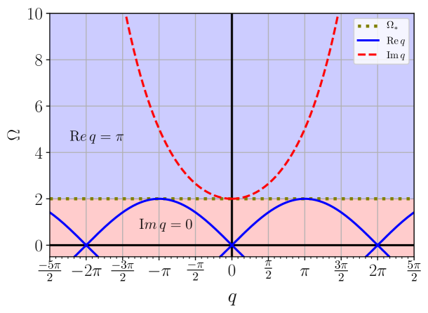
Figure 1: Dispersion relation: the real and the imaginary parts of the wave number $q$ versus frequency $\Omega$

5 The Green function in the frequency domain

Consider now Eqs. (3.4), (3.5), wherein

$$u_{n}(t)=U_{n}(\Omega)\,\mathrm{e}^{-\mathrm{i}\Omega t},$$ (5.1)

$$p(t)=\mathrm{e}^{-\mathrm{i}\Omega t}.$$ (5.2)

We substitute expressions (5.1), (5.2) into Eqs. (3.4), (3.5). This yields

$$(-\Omega^{2}+2)U_{n}-U_{n+1}-U_{n-1}=\delta_{n}\big{(}\Omega^{2}(m-1)U_{0}+1\big{)}.$$ (5.3)

The corresponding steady-state solution $U_{n}=\mathcal{G}_{n}$ of the obtained equation is the Green function in the frequency domain for a chain with an isotopic defect. We look for the solution in the following form:

$${U}_{n}=U_{0}(\Omega)\,\mathrm{e}^{\mathrm{i}q|n|\operatorname{sign}\Omega},\quad q=a(\Omega), \Omega\in\mathbb{P};$$ (5.4)

$${U}_{n}=U_{0}(\Omega)\,\mathrm{e}^{\mathrm{i}q|n|},\quad q=\pi+\mathrm{i}b(\Omega), \Omega\in\mathbb{S};$$ (5.5)

where the wave-number $q$ is defined in accordance with Eq. (4.8) and Eqs. (4.14), (4.15) for the pass-band and the stop-band, respectively. Expression (5.4) satisfies the Sommerfeld radiation conditions, whereas Eq. (5.5) satisfies vanishing boundary conditions at infinity. For $|n|\geq 1$ equations from the system (5.3) transform into corresponding homogeneous equations, which are clearly satisfied by exponential functions (5.4), (5.5). To find unknown $U_{0}$ we need to consider the equation corresponding to $n=0$. This yields

$$\mathcal{G}_{n}(\Omega)=\frac{\mathrm{e}^{\mathrm{i}a|n|\operatorname{sign}\Omega}}{-m\Omega^{2}-2\mathrm{e}^{\mathrm{i}a\operatorname{sign}\Omega}+2}, \Omega\in\mathbb{P};$$ (5.6)

$$\mathcal{G}_{n}(\Omega)=\frac{(-1)^{|n|}\mathrm{e}^{-b|n|}}{-m\Omega^{2}+2\mathrm{e}^{-b}+2}, \Omega\in\mathbb{S}.$$ (5.7)

Substituting Eq. (4.8) and Eq. (4.15) into Eq. (5.6) and Eq. (5.7), respectively, yields:

$$\mathcal{G}_{n}(\Omega)=-\frac{\mathrm{e}^{\mathrm{i}|n|\operatorname{sign}\Omega\,\arccos\frac{2-\Omega^{2}}{2}}}{(m-1)\Omega^{2}+\mathrm{i}\Omega\sqrt{4-\Omega^{2}}}, \Omega\in\mathbb{P};$$ (5.8)

$$\mathcal{G}_{n}(\Omega)=\frac{(-1)^{|n|}2^{|n|}}{\Phi^{|n|-1}(\Omega)\big{(}(-m\Omega^{2}+2)\Phi(\Omega)+4\big{)}}, \Omega\in\mathbb{S};$$ (5.9)

where

$$\Phi(\Omega)\stackrel{{\scriptstyle\mbox{\scriptsize def}}}{{=}}\Omega^{2}-2+|\Omega|\sqrt{\Omega^{2}-4}.$$ (5.10)

In the particular case $m=1$ we have obtained the Green function in the frequency domain for a uniform chain:

$$G_{n}(\Omega)\stackrel{{\scriptstyle\mbox{\scriptsize def}}}{{=}}\mathcal{G}_{n}(\Omega)\big{|}_{m=1}.$$ (5.11)

Note that it is easy to see that the cut-off frequency $\Omega_{\ast}=2$ is a resonant frequency for a a uniform chain. The corresponding non-stationary solution grows as $t\to\infty$ hemmer1959dynamic ; slepyan1987energy ; AyzenbergStepanenko2008 ; Abdukadirov_2019 .

6 The spectral problem for the localized mode

Putting $p=0$ and assuming that Eq. (5.1) is fulfilled, consider the steady-state problem concerning the natural localized oscillation of the system described by Eqs. (3.4), (3.5) at positive frequency $\Omega_{0}$. Since we look for a mode with finite energy we require that

$$\sum_{n=-\infty}^{\infty}U_{n}^{2}<\infty,\qquad\sum_{n=-\infty}^{\infty}(U_{n+1}-U_{n})^{2}<\infty$$ (6.1)

and consider the frequencies in the stop-band: $\Omega_{0}\in\mathbb{S}_{+}$. We substitute expression (5.1) into Eqs. (3.4), (3.5). This yields

$$(-\Omega_{0}^{2}+2)U_{n}-U_{n+1}-U_{n-1}=\delta_{n}\Omega_{0}^{2}(m-1)U_{0}.$$ (6.2)

The solution of the above equation can be written as follows:

$$U_{n}=(m-1)\Omega_{0}^{2}G_{n}(\Omega_{0})U_{0},$$ (6.3)

where $G_{n}(\Omega)$ is the Green function for a uniform chain given by Eq. (5.11). Calculating Eq. (6.3) at $n=0$, one can derive the following frequency equation for the frequency $\Omega_{0}$ of the localized mode:

$$\mathcal{G}_{0}^{-1}(\Omega_{0})=0,$$ (6.4)

i.e., $\Omega_{0}$ should be a resonant frequency. The last equation can be equivalently transformed to the following form, which is useful for the further treatment:

$$\frac{1}{2}(m\Omega_{0}^{2}-2)=\mathrm{e}^{-b(\Omega_{0})},$$ (6.5)

where $b(\Omega_{0})>0$ is defined by the right-hand side of Eq. (4.15).

To find the necessary and sufficient condition for the existence of the localized mode, it is useful to consider simultaneously the frequency equation (6.5) and the dispersion equation (4.13). These two equations can be rewritten in the following form:

$$\Omega_{0}^{2}-2=2\cosh b(\Omega_{0}),$$ (6.6)

$$(m-1)\Omega_{0}^{2}=-2\sinh b(\Omega_{0}).$$ (6.7)

One can see that for $m>1$ Eq. (6.7) cannot be fulfilled since $b>0$ due to (5.5). Thus, the localized mode does not exist in this case.

Consider the case $m<1$. For $\Omega_{0}\in\mathbb{S}_{+}$ both Eqs. (6.6), (6.7) can be fulfilled. Squaring Eqs. (6.6), (6.7) and subtracting the second squared equation from the first one, we rewrite the frequency equation in the following equivalent form

$$\Omega_{0}^{2}(\Omega_{0}^{2}m(2-m)-4)=0.$$ (6.8)

The only positive root of this equation is

$$\Omega_{0}=\frac{2}{\sqrt{m(2-m)}}.$$ (6.9)

Now we should verify that $\Omega_{0}$ given by Eq. (6.9) belongs to $\mathbb{S}_{+}$, i.e., $\Omega_{0}>\Omega_{\ast}$. Squaring Eq. (6.9) gets

$$\frac{4}{m(2-m)}>4\quad\Longleftrightarrow\quad(m-1)^{2}>0,$$ (6.10)

which is true. Thus, for all $m<1$ there exists a unique localized mode with frequency $\Omega_{0}$ defined by Eq. (6.9).

The corresponding form of localized oscillation can be found by Eq. (6.3). One has

$$U_{n}=U_{0}(-1)^{|n|}\mathrm{e}^{-b(\Omega_{0})|n|},$$ (6.11)

where $U_{0}$ is an arbitrary constant. Taking into account Eqs. (6.5), (6.9) one gets:

$$U_{n}=U_{0}\left(\frac{-m}{2-m}\right)^{|n|}.$$ (6.12)

7 Asymptotics for the fundamental solution $\mathcal{V}_{n}$ of the deterministic problem

To obtain the expression for the fundamental solution ${\mathcal{U}}_{n}$, we apply the Fourier transform with respect to time $t$ to Eqs. (3.4), (3.5), and obtain in this way Eq. (5.3), wherein $U_{n}$ has the meaning of the Fourier transform with respect to time $t$ of ${\mathcal{U}}_{n}$. The solution of this equation is the Green function $\mathcal{G}_{n}$ given by Eqs. (5.6), (5.7). Now ${\mathcal{U}}_{n}(t)$ can be represented as the inverse Fourier transform:

$${\mathcal{U}}_{n}=\frac{1}{2\pi}\left(\int_{\mathbb{P}}+\int_{\mathbb{S}}\right)\mathcal{G}_{n}(\Omega)\mathrm{e}^{-\mathrm{i}\Omega t}\,\mathrm{d}\Omega={\mathcal{U}}_{n}^{\mathrm{pass}}+{\mathcal{U}}_{n}^{\mathrm{stop}}.$$ (7.1)

Accordingly,

$${\mathcal{V}}_{n}={\mathcal{V}}_{n}^{\mathrm{pass}}+{\mathcal{V}}_{n}^{\mathrm{stop}}=-\frac{\mathrm{i}}{2\pi}\left(\int_{\mathbb{P}}+\int_{\mathbb{S}}\right)\Omega\mathcal{G}_{n}(\Omega)\mathrm{e}^{-\mathrm{i}\Omega t}\,\mathrm{d}\Omega\\ =-\frac{\mathrm{i}}{2\pi}\left(\int_{\mathbb{P}_{+}}+\int_{\mathbb{S}_{+}}\right)\Omega\mathcal{G}_{n}(\Omega)\mathrm{e}^{-\mathrm{i}\Omega t}\,\mathrm{d}\Omega+\mathrm{c.c.}=I_{n}^{\mathrm{pass}}+I_{n}^{\mathrm{stop}}+\mathrm{c.c.}$$ (7.2)

Remark 3

In the case $m<1$, where the localized mode exists (see Sect. 6), the integral (7.2) over the stop-band does not exist in the classical sense due to the poles $\pm\Omega_{0}$ of the Green function $\mathcal{G}_{n}$ on the real axis. The corresponding details on the meaning of the integral in this case are provided in Sect. 7.2. The integrand of (7.1) (but not (7.2)) also has a pole at $\Omega=0$, which corresponds to the chain motion as a whole.

The integrals $I_{n}^{\mathrm{pass}}$ and $I_{n}^{\mathrm{stop}}$ have the structure of a Fourier integral:

$$I=\int A(\Omega)\,\mathrm{e}^{\mathrm{i}\phi(\Omega)t}\,\mathrm{d}\Omega.$$ (7.3)

To estimate them, we use, in what follows, the procedure of asymptotic evaluation for large times based on the method of stationary phase erdelyi1956asymptotic ; Fedoryuk1977 ; temme2014 .

To make the results to be reproducible, we present detailed calculations for all the corresponding asymptotics. For a reader who prefers to skip the details, it is possible to find the most important formulae summarized in Sect. 7.6.

Asymptotics of a Fourier integral is the sum of contributions $I(\Omega_{i})$ from the critical points $\Omega_{i}$:

$$I=\sum_{i}I(\Omega_{i})+O(t^{-\infty}),\qquad t\to\infty;$$ (7.4)

$$I(\Omega_{i})\stackrel{{\scriptstyle\mbox{\scriptsize def}}}{{=}}\int\mathcal{A}(\Omega)\chi_{\Omega_{i}}(\Omega)\mathrm{e}^{\mathrm{i}\phi(\Omega)t}\,\mathrm{d}\Omega.$$ (7.5)

The critical points are stationary points for the phase $\phi(\Omega)$, finite end-points of the integration intervals and singular points for the phase $\phi(\Omega)$ and the amplitude $\mathcal{A}(\Omega)$. Here $\chi_{\Omega_{i}}(\Omega)$ is a neutraliser at $\Omega=\Omega_{i}$ such that $\chi_{\Omega_{i}}(\Omega)\equiv 0$ in a neighbourhood of any $\Omega_{j}$ for $j\neq i$.

Remark 4

Neutraliser temme2014 ; van1948method $\chi_{\Omega_{i}}(\Omega)$ at a critical point $\Omega_{i}$ is a $C_{0}^{\infty}(\mathbb{R})$ function such that $\chi_{\Omega_{i}}(\Omega_{i})=1$, $\chi^{(n)}_{\Omega_{i}}(\Omega_{i})=0$ for $n>1$, and $\chi_{\Omega_{i}}(\Omega)\equiv 0$ outside of a certain neighbourhood of $\Omega_{i}$.

7.1 The case $0<|n|<t$: the contribution from the pass-band

One has:

$$I^{\mathrm{pass}}_{n}=-\frac{\mathrm{i}}{2\pi}\int_{0}^{2}\frac{\mathrm{e}^{\mathrm{i}|n|\arccos\frac{2-\Omega^{2}}{2}-\mathrm{i}\Omega t}}{-(m-1)\Omega-\mathrm{i}\sqrt{4-\Omega^{2}}}\,\mathrm{d}\Omega.$$ (7.6)

Since the contribution from the pass-band describes propagating waves, following to Gavrilov2022ijhmt , we estimate the large-time asymptotics of the right-hand side of Eq. (7.6) at the moving front

$$|n|=wt,\quad w=\mathrm{const},\quad t\to\infty,\quad t\in\mathbb{R},\quad n\in\mathbb{R}$$ (7.7)

considering $n$ as a continuum spatial variable. Here the meaning of the quantity

$$0<w<1$$ (7.8)

is the speed for the observation point. This approach, which is known to us due to Slepyan1972 in context of continuum problems, allows one to describe running waves, wave-fronts, and to describe the wave-field as a whole, in comparison with the evaluation of the corresponding asymptotics at a fixed position. Note that the cases $n=0$ and $n=t$ are considered separately, in Sect. 7.3 and Sect. 7.4, respectively. Denote

$$\phi=w\arccos\frac{2-\Omega^{2}}{2}-\Omega,$$ (7.9)

$$\mathcal{A}^{\mathrm{pass}}(\Omega)\stackrel{{\scriptstyle\mbox{\scriptsize def}}}{{=}}\mathcal{D}^{-1}(\Omega)\stackrel{{\scriptstyle\mbox{\scriptsize def}}}{{=}}\frac{1}{-(m-1)\Omega-\mathrm{i}\sqrt{4-\Omega^{2}}}.$$ (7.10)

Thus,

$$I^{\mathrm{pass}}_{wt}=-\frac{\mathrm{i}}{2\pi}\int_{0}^{2}\mathcal{A}^{\mathrm{pass}}(\Omega)\mathrm{e}^{\mathrm{i}\phi(\Omega)t}\,\mathrm{d}\Omega.$$ (7.11)

The critical points for $I^{\mathrm{pass}}_{wt}$ are the stationary point for $\phi$, where

$$\phi^{\prime}_{\Omega}=0,$$ (7.12)

and the singular end-point $\Omega=\Omega_{\ast}=2$. Note that the contribution $I^{\mathrm{pass}}_{wt}(0)$ from the end-point $\Omega=0$ totally compensates by the complexly conjugated integral over $(-2,0)$, see term $\mathrm{c.c.}$ in Eq. (7.2).

To estimate the contribution from the singular end-point $\Omega=2$, we consider the behaviour of the amplitude $\mathcal{A}^{\mathrm{pass}}(\Omega)$ and the phase $\phi(\Omega)$ at $\Omega\to 2-0$. One has

$$\begin{multlined}\mathcal{A}^{\mathrm{pass}}(\Omega)=\mathcal{A}^{\mathrm{pass}}_{0}+\mathcal{A}^{\mathrm{pass}}_{1/2}\sqrt{2-\Omega}+O(2-\Omega)\\ \qquad=-\frac{1}{2(m-1)}+\frac{\mathrm{i}}{2(m-1)^{2}}\sqrt{2-\Omega}+O(2-\Omega),\end{multlined}\mathcal{A}^{\mathrm{pass}}(\Omega)=\mathcal{A}^{\mathrm{pass}}_{0}+\mathcal{A}^{\mathrm{pass}}_{1/2}\sqrt{2-\Omega}+O(2-\Omega)\\ \qquad=-\frac{1}{2(m-1)}+\frac{\mathrm{i}}{2(m-1)^{2}}\sqrt{2-\Omega}+O(2-\Omega),$$ (7.15)

$$\phi(\Omega)=\pi w-2-2w\sqrt{2-\Omega}+(2-\Omega)+o(2-\Omega).$$ (7.16)

Taking into account the Erdélyi lemma (see Appendix B), wherein $\alpha=1/2$, $\beta=1$, one gets that the contribution $I^{\mathrm{pass}}_{wt}(\Omega_{\ast})$ from the end-point $\Omega=\Omega_{\ast}\equiv 2$ is $O(t^{-2})$ if (7.8) is fulfilled.

Remark 5

In the case $w=0$, which is considered in Sect. 7.3, the last estimation is $O(t^{-1})$ due to Eq. (7.16). This corresponds to the choice $\alpha=1$, $\beta=1$ in the Erdélyi lemma.

The stationary point is the solution of Eq. (7.12):

$$w\left(\arccos\frac{2-\Omega^{2}}{2}\right)^{\prime}_{\Omega}-1=0.$$ (7.17)

Thus, the expression for the stationary point $\Omega_{\mathrm{s}}$ is

$$\Omega_{\mathrm{s}}=2\sqrt{1-w^{2}},$$ (7.18)

and

$$0<\Omega_{\mathrm{s}}<2.$$ (7.19)

One can see that the stationary point exists and unique for all $w$ in interval (7.8). Put

$$\phi_{\mathrm{s}}\stackrel{{\scriptstyle\mbox{\scriptsize def}}}{{=}}\phi(\Omega_{\mathrm{s}})=w\arccos(2w^{2}-1)-2\sqrt{1-w^{2}}=2(w\arccos w-\sqrt{1-w^{2}}).$$ (7.20)

It can be shown that the stationary point $\Omega_{\mathrm{s}}$ is not a degenerate one:

$$\phi^{\prime\prime}=\frac{\Omega w}{4(1-\frac{\Omega^{2}}{4})^{3/2}}>0,$$ (7.21)

$$\phi^{\prime\prime}(\Omega_{\mathrm{s}})=\frac{\sqrt{1-w^{2}}}{2w^{2}},$$ (7.22)

provided that inequalities (7.8) and (7.19) are fulfilled. Now we can apply the formula for the principal term of the contribution from a non-degenerate stationary point $\Omega_{\mathrm{s}}$. One obtains the following asymptotics:

$${\mathcal{V}}_{wt}^{\mathrm{pass}}=I^{\mathrm{pass}}_{wt}(\Omega_{\mathrm{s}})+I^{\mathrm{pass}}_{wt}(\Omega_{\ast})+\mathrm{c.c.}+O(t^{-\infty})=I^{\mathrm{pass}}_{wt}(\Omega_{\mathrm{s}})+\mathrm{c.c.}+O(t^{-2})\\ =-\frac{\mathrm{i}}{\sqrt{2\pi|\phi^{\prime\prime}(\Omega_{\mathrm{s}})|t}}\,\frac{\mathrm{e}^{\mathrm{i}(\phi_{\mathrm{s}}t+\frac{\pi}{4})}}{\mathcal{D}(\Omega_{\mathrm{s}})}+\mathrm{c.c.}+O(t^{-3/2}).$$ (7.23)

Using Eq. (7.10) one gets

$$\operatorname{Re}\mathcal{D}=-(m-1)\Omega_{\mathrm{s}}=-2(m-1)\sqrt{1-w^{2}},$$ (7.24)

$$\operatorname{Im}\mathcal{D}=-\sqrt{4-{\Omega_{\mathrm{s}}^{2}}}=-2w,$$ (7.25)

$$\begin{multlined}|\mathcal{D}|^{2}=4\big{(}(m-1)^{2}(1-w^{2})+w^{2}\big{)}.\end{multlined}|\mathcal{D}|^{2}=4\big{(}(m-1)^{2}(1-w^{2})+w^{2}\big{)}.$$ (7.27)

Hence, one can obtain:

$${\mathcal{V}}_{wt}^{\mathrm{pass}}=-\frac{2}{\sqrt{{2\pi}\phi^{\prime\prime}_{\mathrm{s}}t}}\frac{1}{|\mathcal{D}|^{2}}\bigg{(}\operatorname{Im}\mathcal{D}\cos\Big{(}\phi_{\mathrm{s}}t+\frac{\pi}{4}\Big{)}-\operatorname{Re}\mathcal{D}\sin\Big{(}\phi_{\mathrm{s}}t+\frac{\pi}{4}\Big{)}\bigg{)}+O(t^{-3/2})\\ =-\frac{1}{\sqrt{\pi t}}\frac{w\Big{(}-w\cos\Big{(}\phi_{\mathrm{s}}t+\frac{\pi}{4}\Big{)}+(m-1)\sqrt{1-w^{2}}\sin\Big{(}\phi_{\mathrm{s}}t+\frac{\pi}{4}\Big{)}\Big{)}}{{(1-w^{2})^{1/4}}\big{(}(m-1)^{2}(1-w^{2})+w^{2}\big{)}}+O(t^{-3/2})\\ =\frac{1}{\sqrt{\pi t}}\frac{w\cos\left(\phi_{\mathrm{s}}t+\psi+\frac{\pi}{4}\right)}{{(1-w^{2})^{1/4}}\big{(}(m-1)^{2}(1-w^{2})+w^{2}\big{)}^{1/2}}+O(t^{-3/2}),$$ (7.28)

where

$$\psi=\arctan\frac{\operatorname{Re}\mathcal{D}}{\operatorname{Im}\mathcal{D}}=\arctan\frac{(m-1)\sqrt{1-w^{2}}}{w}.$$ (7.29)

Now we return to variables $n$, $t$, and substitute $w=|n|/t$ into the last expression. This yields:

$${\mathcal{V}}_{|n|=wt}^{\mathrm{pass}}=-\frac{|n|}{\sqrt{\pi}(t^{2}-n^{2})^{1/4}\big{(}(m-1)^{2}(t^{2}-n^{2})+n^{2}\big{)}}\\ \times\Big{(}-|n|\cos\Big{(}\phi_{\mathrm{s}}t+\frac{\pi}{4}\Big{)}+(m-1)\sqrt{t^{2}-n^{2}}\sin\Big{(}\phi_{\mathrm{s}}t+\frac{\pi}{4}\Big{)}\Big{)}+O(t^{-3/2})\\ =\frac{|n|}{\pi^{1/2}(t^{2}-n^{2})^{1/4}\left((m-1)^{2}(t^{2}-n^{2})+n^{2}\right)^{1/2}}\cos\left(\phi_{\mathrm{s}}t+\psi+\frac{\pi}{4}\right)+O(t^{-3/2}),$$ (7.30)

where according to Eqs. (7.20), (7.29)

$$\phi_{\mathrm{s}}=2\left(\frac{|n|}{t}\arccos\frac{|n|}{t}-\frac{\sqrt{t^{2}-n^{2}}}{t}\right),$$ (7.31)

$$\psi=\arctan\frac{(m-1)\sqrt{t^{2}-n^{2}}}{|n|}.$$ (7.32)

7.2 The contribution from the stop-band

One has:

$$I_{n}^{\mathrm{stop}}=-\frac{\mathrm{i}}{2\pi}\int_{2}^{\infty}\frac{(-1)^{|n|}\,\Omega\,\mathrm{e}^{-b(\Omega)|n|-\mathrm{i}\Omega t}}{-m\Omega^{2}+2\mathrm{e}^{-b(\Omega)}+2}\,\mathrm{d}\Omega.$$ (7.33)

The contribution from the stop-band describes non-propagating exponentially vanishing as $n\to\infty$ waves. Therefore, we estimate the large-time asymptotics of the right-hand side of Eq. (7.33) at a fixed spatial position $n$.

While evaluating the contribution from the stop-band, we have two qualitatively different cases, namely, the case of a heavy defect ($m>1$) and the case of a light defect ($m<1$). Indeed, the localized mode exists in the system if and only if $m<1$ (see Sect. 6). The frequency of localized oscillation is a root of frequency equation (6.4). Thus, the pole $\Omega=\Omega_{0}$ exists inside the integration interval $\mathbb{S}_{+}$ if and only if $m<1$.

In the case $m>1$ there is no pole and integral (7.33) exists in the classical sense. The only critical point for the integral is the cut-off frequency $\Omega_{\ast}=2$:

$$I_{n}^{\mathrm{stop}}=I_{n}^{\mathrm{stop}}(\Omega_{\ast})+O(t^{-\infty}).$$ (7.34)

A rough estimation $I_{n}^{\mathrm{stop}}(\Omega_{\ast})=O(t^{-1})$ can be obtained from the Erdélyi lemma with $\alpha=1$, $\beta=1$. Thus, in the case of a heavy defect $m>1$ one has

$${\mathcal{V}}_{n}^{\mathrm{stop}}=O(t^{-1}).$$ (7.35)

In the case $m<1$ there is the pole $\Omega_{\mathrm{s}}\in\mathbb{S}_{+}$ and integral (7.33) does not exist in the classical sense. In the latter case the integral in the right-hand side of (7.33) should be considered as the Fourier transform for a generalized function. To get the possibility to deal with the right-hand side of (7.33) as an ordinary Lebesgue integral we use the limit absorption principle. We add the dissipative viscous term into governing equation (3.1), repeat all the calculations and find the root of the denominator for the right-hand side of Eq. (3.1) modified in such a way (see Gavrilov1999jsv for details). Then we consider a limiting case of zero dissipation to define the positions of the poles with respect to the real axis. One can show that the poles are shifted into the lower half-plane of the complex plane: $\Omega=\pm\Omega_{0}-\mathrm{i}0$. To calculate the contribution $I_{n}^{\mathrm{stop}}(\Omega_{0})$ we apply Sokhotski–Plemelj theorem for the real line Vladimirov1971 :

$$\int_{-\infty}^{\infty}\frac{\bar{f}(\Omega)}{\Omega\pm\mathrm{i}0}\,\mathrm{d}\Omega=\mp\mathrm{i}\pi f(0)+\operatorname{PV}\int_{-\infty}^{\infty}\frac{\bar{f}(\Omega)}{\Omega}\,\mathrm{d}\Omega,$$ (7.36)

and the following asymptotic formula Fedoryuk1977 for the asymptotics of the Cauchy principal value for the integral

$$\operatorname{PV}\int_{-\infty}^{\infty}\frac{f(\Omega)\,e^{-\mathrm{i}\Omega t}}{\Omega}\,\mathrm{d}\Omega=-\pi\mathrm{i}\,f(0)+O(t^{-\infty}).$$ (7.37)

Here $\bar{f}(\Omega),f(\Omega)\in C_{0}^{\infty}$. Now one can put

$$\bar{f}(\Omega)=f(\Omega)\,\mathrm{e}^{-\mathrm{i}\Omega t}$$ (7.38)

and use Eq. (7.36). This yields

$$\int_{-\infty}^{\infty}\frac{f(\Omega)\,e^{-\mathrm{i}\Omega t}}{\Omega-\mathrm{i}0}\,d\Omega=O(t^{-\infty}),$$ (7.39)

$$\int_{-\infty}^{\infty}\frac{f(\Omega)\,e^{-\mathrm{i}\Omega t}}{\Omega+\mathrm{i}0}\,d\Omega=-2\pi\mathrm{i}\,f(0)+O(t^{-\infty}).$$ (7.40)

Using Eq. (7.40), one gets

$$\int_{-\infty}^{\infty}\frac{f(\Omega)\,e^{-\mathrm{i}\Omega t}}{\Omega-\Omega_{0}+\mathrm{i}0}\,d\Omega=-2\pi\mathrm{i}\,f(\Omega_{0})\,e^{-\mathrm{i}\Omega_{0}t}+O(t^{-\infty})\\ =-2\pi\mathrm{i}\,\operatorname{Res}\big{(}F(\Omega),\Omega_{0}\big{)}\,e^{-\mathrm{i}\Omega_{0}t}+O(t^{-\infty}).$$ (7.41)

The last equality is correct provided that $F(\Omega)=f(\Omega)/(\Omega-\Omega_{0})$ is an analytic function in a neighbourhood of $\Omega_{0}$.

Applying Eq. (7.41) one obtains

$$I_{n}^{\mathrm{stop}}(\Omega_{0})=I_{0}^{\mathrm{stop}}(\Omega_{0})(-1)^{|n|}\mathrm{e}^{-b(\Omega_{0})|n|},$$ (7.42)

$$I_{0}^{\mathrm{stop}}(\Omega_{0})=-{\Omega_{0}}\operatorname{Res}\left(\frac{1}{-m\Omega^{2}+2\mathrm{e}^{-b}+2},{\Omega_{0}}\right)\mathrm{e}^{-\mathrm{i}{\Omega_{0}}t}+O(t^{-\infty}),$$ (7.43)

where

$$\operatorname{Res}\left(\frac{1}{-m\Omega^{2}+2\mathrm{e}^{-b}+2},\Omega_{0}\right)=\frac{1}{-2m\Omega-2b^{\prime}_{\Omega}\mathrm{e}^{-b}}\\ =\frac{\sinh b}{\Omega_{0}(-m\mathrm{e}^{b}+(m-2)\mathrm{e}^{-b})}=-\frac{(m-1)\Omega_{0}}{2\big{(}m(m-2)\Omega_{0}^{2}+2\big{)}}.$$ (7.44)

Here, to simplify the left-hand side of (7.44) we have used relation

$$b^{\prime}_{\Omega}=\frac{\Omega}{\sinh b(\Omega)},$$ (7.45)

which follows from Eq. (6.6). Also, we have used Eq. (6.5) to calculate $\exp(-b)$ and Eq. (6.7) to calculate $\sinh b$. Using Eqs. (6.5), (6.9) one finally obtains:

$${\mathcal{V}}_{n}^{\mathrm{stop}}=\frac{(m-1)(-1)^{|n|+1}m^{|n|-1}}{(2-m)^{|n|+1}}\mathrm{e}^{-\mathrm{i}\Omega_{0}t}+I_{n}^{\mathrm{stop}}(\Omega_{\ast})+O(t^{-\infty})+\mathrm{c.c.},$$ (7.46)

where $I_{n}^{\mathrm{stop}}(\Omega_{\ast})=O(t^{-1})$. Finally,

$${\mathcal{V}}_{n}^{\mathrm{stop}}=\frac{2(m-1)(-1)^{|n|+1}m^{|n|-1}}{(2-m)^{|n|+1}}\cos\Omega_{0}t+O(t^{-1}).$$ (7.47)

Formula (7.47) describes non-vanishing localized oscillation, which exists in the case of a light defect $m<1$. For the first time this result was obtained in Kashiwamura1962 .

7.3 The case $n=0$: the contribution from the cut-off frequency

Consider the case $w=0$, which corresponds to a fixed position $n=0$. In this case the stationary point $\Omega_{\mathrm{s}}$ collocates with the cut-off frequency: ($\Omega_{\mathrm{s}}\to\Omega_{\ast}-0$ as $w\to+0$), and disappears. Accordingly, the term of order $t^{-1/2}$ of the asymptotics for ${\mathcal{V}}_{0}^{\mathrm{pass}}$ vanishes, see Eq. (7.28). In this section we estimate the principal term for

$$I_{0}(\Omega_{\ast})+\mathrm{c.c.}=I_{0}^{\mathrm{pass}}(\Omega_{\ast})+I_{0}^{\mathrm{stop}}(\Omega_{\ast})+\mathrm{c.c.}$$ (7.48)

Due to Eqs. (7.5), (7.11) one has

$$I^{\mathrm{pass}}_{0}(\Omega_{\ast})=-\frac{\mathrm{i}}{2\pi}\int_{-\infty}^{2}\chi_{2}(\Omega)\mathcal{A}^{\mathrm{pass}}(\Omega)\mathrm{e}^{-\mathrm{i}\Omega t}\,\mathrm{d}\Omega,$$ (7.49)

where $\chi_{2}(\Omega)$ is a neutralizer (see Remark 7), and expansion (7.15) is valid for $\Omega\to\Omega_{\ast}-0$. On the other hand, due to Eqs. (7.5), (7.33)

$$I_{0}^{\mathrm{stop}}(\Omega_{\ast})=-\frac{\mathrm{i}}{2\pi}\int_{2}^{\infty}\chi_{2}(\Omega)\mathcal{A}^{\mathrm{stop}}(\Omega)\mathrm{e}^{-\mathrm{i}\Omega t}\,\mathrm{d}\Omega,$$ (7.50)

$$\mathcal{A}^{\mathrm{stop}}\stackrel{{\scriptstyle\mbox{\scriptsize def}}}{{=}}\frac{\Omega}{-m\Omega^{2}+2\mathrm{e}^{-b}+2}.$$ (7.51)

One can show that

$$\mathcal{A}^{\mathrm{stop}}=\mathcal{A}^{\mathrm{stop}}_{0}+\mathcal{A}^{\mathrm{stop}}_{1/2}\sqrt{\Omega-2}+o(\sqrt{\Omega-2})\\ =-\frac{1}{2(m-1)}+\frac{1}{2(m-1)^{2}}\sqrt{\Omega-2}+o(\sqrt{\Omega-2}),\quad\Omega\to 2+0.$$ (7.52)

Since $\mathcal{A}_{0}^{\mathrm{pass}}=\mathcal{A}_{0}^{\mathrm{stop}}$,

$$\underbrace{\int_{-\infty}^{2}\chi_{2}(\Omega)\mathcal{A}_{0}^{\mathrm{pass}}(\Omega)\,\mathrm{e}^{-\mathrm{i}\Omega t}\,\mathrm{d}\Omega}_{J}+\int_{2}^{\infty}\chi_{2}(\Omega)\mathcal{A}_{0}^{\mathrm{stop}}(\Omega)\,\mathrm{e}^{-\mathrm{i}\Omega t}\,\mathrm{d}\Omega=O(t^{-\infty}).$$ (7.53)

Applying the Erdélyi lemma with $\alpha=1,\ \beta=3/2$ yields

$$I_{0}^{\mathrm{pass}}(\Omega_{\ast})=J+\frac{1}{2\pi}\int_{0}^{\infty}\big{(}|\mathcal{A}^{\mathrm{pass}}_{1/2}|\sqrt{\mu}+o(\sqrt{\mu})\big{)}\mathrm{e}^{\mathrm{i}(\mu-2)t}\,\mathrm{d}\mu+\mathrm{c.c.}+O(t^{-\infty})\\ =2\operatorname{Re}J+2\operatorname{Re}\frac{|\mathcal{A}^{\mathrm{pass}}_{1/2}|\Gamma\left(\frac{3}{2}\right)\mathrm{e}^{\mathrm{i}\left(2t-\frac{3\pi}{4}\right)}}{2\pi\,t^{3/2}}+o(t^{-3/2})\\ =2\operatorname{Re}J+\frac{\cos\left(2t-\frac{3\pi}{4}\right)}{4\sqrt{\pi}(m-1)^{2}\,t^{3/2}}+o(t^{-3/2}),$$ (7.54)

$$I_{0}^{\mathrm{stop}}(\Omega_{\ast})=-J-\frac{\mathrm{i}}{2\pi}\int_{0}^{\infty}\big{(}\mathcal{A}^{\mathrm{stop}}_{1/2}\sqrt{\mu}+o(\sqrt{\mu})\big{)}\mathrm{e}^{-\mathrm{i}(2+\mu)t}\,\mathrm{d}\mu+\mathrm{c.c.}+O(t^{-\infty})\\ =-2\operatorname{Re}J+2\operatorname{Re}\frac{\mathcal{A}^{\mathrm{stop}}_{1/2}\Gamma\left(\frac{3}{2}\right)\mathrm{e}^{\mathrm{i}\left(2t+\frac{3\pi}{4}+\frac{\pi}{2}\right)}}{2\pi\,t^{3/2}}+o(t^{-3/2})\\ =-2\operatorname{Re}J+\frac{\cos\left(2t-\frac{3\pi}{4}\right)}{4\sqrt{\pi}(m-1)^{2}\,t^{3/2}}+o(t^{-3/2}).$$ (7.55)

Here relation

$$\Gamma\left(\frac{3}{2}\right)=\frac{\sqrt{\pi}}{2}$$ (7.56)

is taken into account. Finally, one has

$${\mathcal{V}}_{0}=I_{0}^{\mathrm{stop}}(\Omega_{0})H(1-m)+\frac{\cos\left(2t-\frac{3\pi}{4}\right)}{2\sqrt{\pi}(m-1)^{2}\,t^{3/2}}+o(t^{-3/2}).$$ (7.57)

Here $I_{0}^{\mathrm{stop}}(\Omega_{0})$ is defined by Eqs. (7.43), (7.44) in the case of a light defect. Formula (7.57) was previously obtained in Rubin_1963 .

7.4 The case $|n|=t$

One has $\Omega_{\mathrm{s}}\to+0$ as $w\to 1$, therefore for $w=1$ two stationary points collocate:

$$\phi^{\prime\prime}\big{|}_{\Omega_{\mathrm{s}}=0}=0,\qquad\phi^{\prime\prime\prime}\big{|}_{\Omega_{\mathrm{s}}=0}=\frac{1}{4}.$$ (7.58)

The principal term of the asymptotics on the front $w=1$ ($n=\pm t$) can now be calculated by the Erdélyi lemma, wherein $\alpha=1/3$, $\beta=1$:

$${\mathcal{V}}^{\mathrm{pass}}_{\pm t}=-\frac{\mathrm{i}}{2\pi}\int_{-2}^{2}\chi_{0}(\Omega)\big{(}\mathcal{A}^{\mathrm{pass}}(0)+o(1)\big{)}\mathrm{e}^{\mathrm{i}t\left(\frac{\phi^{\prime\prime\prime}(0)\Omega^{3}}{6}+o(1)\right)}\,\mathrm{d}\Omega+O(t^{-\infty})\\ =\frac{\Gamma(\frac{1}{3})}{2\cdot 3^{1/6}\pi}\,t^{-1/3}+o\big{(}t^{-1/3}\big{)}.$$ (7.59)

Thus, the principal term for the particle velocity on the leading front $|n|=t$ does not depend on $m$, and coincides with the corresponding result for the uniform chain.

More detailed uniform asymptotics describing the behaviour of ${\mathcal{V}}_{n\simeq|t|}^{\mathrm{pass}}$ in a certain neighbourhood of the leading wave front $n=\pm t$ can be obtained by considering collocations of the stationary points $\pm\Omega_{s}\simeq 0$. This solution can be expressed in terms of the Airy function Fedoryuk1977 ; temme2014 .

7.5 The case $|n|>t$

In the case (7.7) wherein $w>1$ the only critical points for $I^{\mathrm{pass}}_{wt}$ is the singular end-point $\Omega=\Omega_{\ast}=2$. The corresponding contribution can be estimated in the same way as in Sect. 7.1 as $O(t^{-2})$. On the other hand, the integral $I^{\mathrm{stop}}_{wt}$ is not a Fourier integral any more, and thus it cannot be evaluated by the stationary phase method. We expect that

$${\mathcal{V}}_{wt}=I^{\mathrm{pass}}_{wt}+I^{\mathrm{stop}}_{wt}+\mathrm{c.c.}=O(t^{-\infty})$$ (7.60)

as well as it is observed in the uniform chain, where this result follows from the exact analytic solution in terms of Bessel functions Olver1997 ; Sokolov2021 . Note that numerical calculations are in agreement with this hypothesis. Nevertheless, there we do not see an easy way to prove asymptotics (7.60) in the case $m\neq 1$ basing on integral representation (7.2).

7.6 Summary: the approximate solution

Let us summarize the results obtained in Sect. 7. According to Eqs. (7.30), (7.47) the approximate solution ${v}_{n}$: ${v}_{n}\simeq{\mathcal{V}}_{n}$, which we use in Sect. 8 to investigate thermal motions, is

$${v}_{n}\stackrel{{\scriptstyle\mbox{\scriptsize def}}}{{=}}{v}_{n}^{\mathrm{pass}}, m>1;$$ (7.61)

$${v}_{n}\stackrel{{\scriptstyle\mbox{\scriptsize def}}}{{=}}{v}_{n}^{\mathrm{pass}}+{v}_{n}^{\mathrm{stop}}, 0<m<1;$$ (7.62)

where

$${v}_{n}^{\mathrm{pass}}\stackrel{{\scriptstyle\mbox{\scriptsize def}}}{{=}}\frac{H(t-|n|)\,|n|}{\pi^{1/2}(t^{2}-n^{2})^{1/4}\left((m-1)^{2}(t^{2}-n^{2})+n^{2}\right)^{1/2}}\cos\left(\phi_{\mathrm{s}}t+\psi+\frac{\pi}{4}\right),$$ (7.63)

$${v}_{n}^{\mathrm{stop}}=\frac{2(m-1)(-1)^{|n|+1}m^{|n|-1}}{(2-m)^{|n|+1}}\cos\Omega_{0}t.$$ (7.64)

Here $\phi_{\mathrm{s}}$ and $\psi$ are defined by Eqs. (7.31) and (7.32), respectively.

Remark 6

By construction (see Eq. (7.7)), quantity ${v}_{n}^{\mathrm{pass}}$ in Eq. (7.63) can be considered as a continuum one ($n\in\mathbb{R}$), which is equal to the particle velocity of a particle with number $n$ for $n\in\mathbb{Z}$. On the other hand, $n\in\mathbb{Z}$ in Eq. (7.64) for ${v}_{n}^{\mathrm{stop}}$, since for the localized mode neighbouring particles oscillate in counter phase.

Formula (7.61) has an exact asymptotic meaning. For $|n|<t$, $n\neq 0$, the right-hand side coincides with the principal term of order $t^{-1/2}$ for the asymptotics on the moving front $|n|=wt$. For $|n|>t$ we expect that the corresponding asymptotics is $O(t^{-\infty})$, see Sect. 7.5. For $w=0$ (or $n=0$) the principal term is of order $t^{-3/2}$ and defined by Eq. (7.57). For $w=1$ (or $|n|=t$) the principal term is of order $t^{-1/3}$ and defined by Eq. (7.59).

Formula (7.62) is not asymptotically correct, since two terms in the right-hand side are asymptotics calculated at a moving position and at a fixed one, respectively. Formula (7.63) describes decaying with the time propagating component of the wave-field, which exists for any positive value of $m$. Formula (7.64) describes non-vanishing localized oscillation, which exists in the case of a light defect $0<m<1$.

8 Numerics

The obtained analytical results were compared with the results of the of numerical integration of $N=2n+1$ ODE (3.1) with periodic conditions at the ends of the chain.

In Fig. 2 we compare the approximate solution $v_{n}$ in the form of Eqs. (7.61)–(7.64) and the corresponding numerical solution in the cases of a heavy defect and a light one (particle velocities versus particle numbers). We also demonstrate the corresponding exact solution (3.11) for a uniform chain at the same plot. One can clearly observe the effects of anti-localization (for the both heavy and light defects) and localization (for the case of a light defect). The obtained analytical solution is in a good agreement with the numerical one everywhere excepting the wave front $|n|=t$. Remember, that solution (7.61)–(7.64) is not valid by construction near $|n|=t$ (see Sect. 7.4). At the leading wave front asymptotics (7.59) should be used instead. The corresponding value is also marked at the plot to demonstrate a good agreement.

In Fig. 3 we provide the analogous comparison for particle velocities versus time. One can observe the vanishing oscillation in the case of a heavy defect and undamped non-vanishing oscillation in case of a light defect. Finally, in Fig. 4 we compare in the case of a heavy defect the asymptotic solution (7.57) for ${\mathcal{V}}_{0}(t)$ with the corresponding numerical results and demonstrate a good agreement.

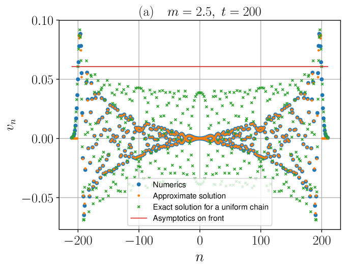
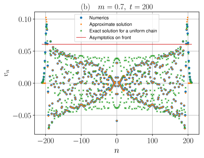
Figure 2: Comparing the approximate solution $v_{n}$ in the form of Eqs. (7.61)–(7.64) and numerical solution (particle velocities versus particle numbers). (a) The case of heavy defect, (b) the case of a light defect. The green crosses correspond to the corresponding exact solution (3.11) for a uniform chain. The red solid line corresponds to the value of $v_{n}$ given by Eq. (7.59) on the leading front $|n|=t$

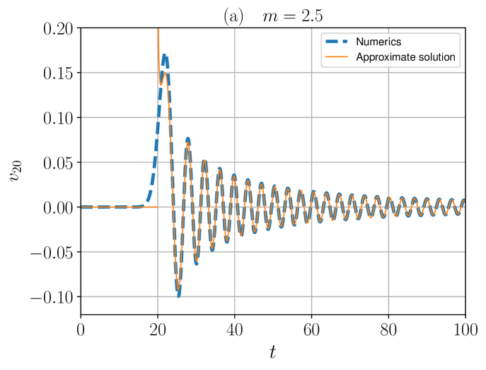
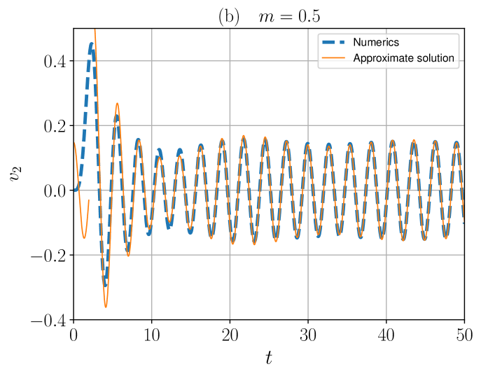
Figure 3: Comparing the approximate solution $v_{n}$ in the form of Eqs. (7.61)–(7.64) and numerical solution (particle velocity versus time). (a) The case of a heavy defect, (b) the case of a light defect

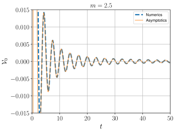
Figure 4: Comparing the asymptotics for $\mathcal{V}_{0}$ in the form of Eq. (7.57) and numerical solution (particle velocity versus time) in the case of heavy defect

9 Discussion: the cases of a light defect, a heavy one, and a uniform chain

Put $m=1$ in the approximate solutions for $m>1$ or $m<1$ (Eq. (7.61) or Eq. (7.62), respectively). This yields

$${v}_{n}={v}_{n}^{\mathrm{pass}}=\frac{H(t-|n|)\,|n|}{\pi^{1/2}(t^{2}-n^{2})^{1/4}|n|}\cos\left(\phi_{\mathrm{s}}t+\frac{\pi}{4}\right).$$ (9.1)

For $n\neq 0$ we can drop $|n|$ in the numerator and the denominator and get the expression

$${v}_{n}=\frac{{H(t-|n|)}}{\pi^{1/2}(t^{2}-n^{2})^{1/4}}\cos\left(\phi_{\mathrm{s}}t+\frac{\pi}{4}\right).$$ (9.2)

The last expression was previously obtained Gavrilov2022ijhmt as the principal term for the asymptotics of the exact analytic solution for the problem concerning a uniform chain. Thus, for $n\not=0$ the approximate solution for $m>1$ or $m<1$ (Eq. (7.61) or Eq. (7.62), respectively) transforms into the approximate solution for the uniform chain.

In the case of a heavy defect $m>1$ the approximate solution (7.63) is zero at $n=0$ (and this is not true for the uniform chain, see Eq. (9.2)). Speaking more accurately, this fact means that the principal term of the asymptotic solution for $w=0$ is of order $O(t^{-3/2})$ and described by Eq. (7.57), whereas it is of order $O(t^{-1/2})$ in a uniform chain. Such a result and the corresponding asymptotics (7.57) was obtained in the paper by Rubin Rubin_1963 and is in agreement with results obtained in Kashiwamura1962 ; Mueller1962 . Moreover, the similar result was obtained by Kaplunov kaplunov1986torsional , who considered a continuum system with a point inertial inclusion, where a localized (trapped) mode exists. We suggest to call this phenomenon “anti-localization”. The physical meaning of anti-localization is a tendency for the unsteady propagating wave-field to avoid a neighbourhood of an inclusion or a defect.

In the case of a light defect $0<m<1$ the non-stationary localized oscillation exists and dominates over all other motions for small $n$. A part of the total energy of the chain is trapped near the defect. Note that the propagating part of the wave-field is also anti-localized.

In the case $m\simeq 1,\ m\neq 1$ the obtained approximate solution (7.61)–(7.64), as well as formula (7.57), become applicable at small $n$ after a very large time. This is because two or three critical points, namely the stationary point $\Omega_{\mathrm{s}}$ defined by Eq. (7.18), the cut-off frequency $\Omega_{\ast}=2$, and the pole $\Omega_{0}$ in the case $m<1$:

$$\Omega_{0}=2+(m-1)^{2}+O\big{(}(m-1)^{3}\big{)},\qquad m\to 1-0,$$ (9.3)

collocate as $n=0\ (w=0)$ and $m\to 1-0$. To describe this case better one needs to consider the collocations and to obtain the corresponding uniform asymptotics. This is a separate difficult problem, which is beyond the scope of the current paper.

Remark 7

Put $|m-1|=1$ in Eq. (7.63). This yields

$${v}_{n}^{\mathrm{pass}}=\frac{H(t-|n|)\,|n|}{\pi^{1/2}(t^{2}-n^{2})^{1/4}t}\cos\left(\phi_{\mathrm{s}}t+\frac{\pi}{4}\right).$$ (9.4)

For $\frac{|n|}{t}\sim 1$ the right-hand side of Eq. (9.4) coincides with the right-hand side of Eq. (9.2) obtained for the uniform chain. The corresponding asymptotics in the case $m=2$ was obtained by Rubin in Rubin_1963 , and, strictly speaking, it is incorrect, because (7.63) is inapplicable for $\frac{|n|}{t}\sim 1$ due to singularities collocation (see Sect. 7.4). This result and formula (7.57) are only results concerning to propagating part of the wave-field, which obtained in the paper by Rubin Rubin_1963 , who estimated the integral representation of the solution at a fixed position.

10 The thermal motion

In this section we investigate the properties of the thermal fundamental solution $\mathcal{T}_{n}$ defined by (3.20). To do this we use the approximation $v_{n}$ defined by Eqs. (7.62)–(7.64) for the fundamental solution ${\mathcal{V}}_{n}$ and obtain:

$$\mathcal{T}_{n}\simeq 2mm_{n}{v}_{n}^{2}(t).$$ (10.1)

At first, consider the case $m>1$. One has ${v}_{n}={v}_{n}^{\mathrm{pass}}$ due to Eq. (7.61), where ${v}_{n}^{\mathrm{pass}}$ is defined by Eq. (7.63) for $n\in\mathbb{R}$ (see Remark 6). Since ${v}_{0}^{\mathrm{pass}}=0$, the right-hand side of Eq. (10.1) can be in a natural way rewritten as a smooth continuum quantity

$$\mathcal{T}_{n}\simeq 2m{v}_{n}^{2}(t),\quad n\in\mathbb{R}.$$ (10.2)

Thus,

$$\mathcal{T}_{n}\simeq\mathcal{T}_{n}^{\mathrm{pass}}\stackrel{{\scriptstyle\mbox{\scriptsize def}}}{{=}}\frac{2m|n|^{2}\cos^{2}\left(\phi_{\mathrm{s}}t+\psi+\frac{\pi}{4}\right)H(t-|n|)}{\pi(t^{2}-n^{2})^{1/2}\left((m-1)^{2}(t^{2}-n^{2})+n^{2}\right)}=\bar{\mathcal{T}}_{n}^{\mathrm{pass}}+\hat{\mathcal{T}}_{n}^{\mathrm{pass}},\qquad n\in\mathbb{R},$$ (10.3)

where

$$\bar{\mathcal{T}}_{n}^{\mathrm{pass}}\stackrel{{\scriptstyle\mbox{\scriptsize def}}}{{=}}\frac{mn^{2}H(t-|n|)}{\pi(t^{2}-n^{2})^{1/2}\big{(}(m-1)^{2}(t^{2}-n^{2})+n^{2}\big{)}},$$ (10.4)

$$\hat{\mathcal{T}}_{n}^{\mathrm{pass}}\stackrel{{\scriptstyle\mbox{\scriptsize def}}}{{=}}-\bar{\mathcal{T}}_{n}^{\mathrm{pass}}\sin 2(\phi_{\mathrm{s}}t+\psi).$$ (10.5)

Formula (10.3) yields the asymptotic decoupling of thermal fundamental solution $\mathcal{T}_{n}$ as the sum of the slow $\bar{\mathcal{T}}_{n}^{\mathrm{pass}}$ and the fast $\hat{\mathcal{T}}_{n}^{\mathrm{pass}}$ motions, which are considered as continuum quantities. Thus, Eqs. (10.3), (10.4), (10.5), provide a natural continuum description of the thermal motions in the system under consideration.

Remark 8

Formulae (10.4), (10.5) for all $n\neq 0$ transform as $m\to 1$ into the expressions for the slow and the fast motions, respectively, in a uniform chain. The last expressions are obtained in Gavrilov2022ijhmt using the asymptotic estimation of an integral representation for the exact solution in the explicit form (3.11) at a moving point of observation.

Remark 9

In study Kuzkin-Krivtsov-accepted an alternative procedure of uncoupling of the slow and the fast motions was suggested for the case of an arbitrary uniform scalar harmonic lattice. In the case of a uniform chain, our approach leads to the same expression for the slow motion, and different expression for the fast motion. Apparently, the result of Kuzkin-Krivtsov-accepted related with the fast motion can be obtained by calculation of the discrete convolution of the fundamental solution $\mathcal{T}_{n}$ in the form of Eq. (10.3) with a slowly spatially-varying discrete function describing initial conditions for the particle velocity. Nevertheless, this issue requires an additional investigation.

Remark 10

In the particular case $m=1$ formula (10.4) coincides for $n\neq 0$ with the solution of the ballistic heat equation introduced in krivtsov2015heat ; krivtsov-da70 , which provides continuum description of heat transport in a uniform chain. The corresponding formula in this particular case also can be found in recent study Allen2022 , where an alternative approach to continuum description of heat transport in a uniform chain is suggested.

Remark 11

Since the term of order $t^{-1/2}$ for the expansion of ${\mathcal{V}}_{n}^{\mathrm{pass}}$ (7.30) and the approximate solution ${v}_{n}^{\mathrm{pass}}$ (7.63) are zeros for $n=0$, strictly speaking, we should use Eq. (7.57) instead. This yields:

$$\bar{\mathcal{T}}_{0}=\frac{m^{2}}{4\pi(m-1)^{4}\,t^{3}}+o(t^{-3}).$$ (10.6)

In the case $m<1$ due to (7.62) one has

$$({v}_{n})^{2}=({v}^{\mathrm{pass}}_{n})^{2}+({v}^{\mathrm{stop}}_{n})^{2}+2{v}^{\mathrm{pass}}_{n}{v}^{\mathrm{stop}}_{n},$$ (10.7)

and, therefore,

$$\mathcal{T}_{n}\simeq\mathcal{T}_{n}^{\mathrm{pass}}+\mathcal{T}_{n}^{\mathrm{stop}}+\mathcal{T}_{n}^{\mathrm{cross}},$$ (10.8)

where the first term $\mathcal{T}_{n}^{\mathrm{pass}}$ is defined by Eq. (10.3). Calculating the second term $\mathcal{T}_{n}^{\mathrm{stop}}$ using (7.64), one gets

$$({v}^{\mathrm{stop}}_{n})^{2}=\frac{2(m-1)^{2}m^{2(|n|-1)}}{(2-m)^{2(|n|+1)}}(1+\cos 2\Omega_{0}t).$$ (10.9)

Hence,

$$\mathcal{T}_{n}^{\mathrm{stop}}=\bar{\mathcal{T}}_{n}^{\mathrm{stop}}+\hat{\mathcal{T}}_{n}^{\mathrm{stop}},$$ (10.10)

$$\bar{\mathcal{T}}_{n}^{\mathrm{stop}}\stackrel{{\scriptstyle\mbox{\scriptsize def}}}{{=}}\frac{4m_{n}(m-1)^{2}m^{2|n|-1}}{(2-m)^{2(|n|+1)}},$$ (10.11)

$$\hat{\mathcal{T}}_{n}^{\mathrm{stop}}\stackrel{{\scriptstyle\mbox{\scriptsize def}}}{{=}}\bar{\mathcal{T}}_{n}^{\mathrm{stop}}\cos 2\Omega_{0}t.$$ (10.12)

Remark 12

Expression (10.11) for the slow motion $\bar{\mathcal{T}}_{n}^{\mathrm{stop}}$ can be continualized by a natural way in the range $|n|\geq 1$, where $m_{n}=1$.

Finally, for the cross product term $\mathcal{T}_{n}^{\mathrm{cross}}$ one gets

$$\mathcal{T}_{n}^{\mathrm{cross}}\stackrel{{\scriptstyle\mbox{\scriptsize def}}}{{=}}4mm_{n}{v}_{n}^{\mathrm{pass}}{v}_{n}^{\mathrm{stop}}$$ (10.13)

and, therefore,

$$\mathcal{T}^{\mathrm{cross}}_{n}=\frac{8m_{n}|n|(m-1)(-1)^{|n|+1}m^{|n|}\,\cos\left(\phi_{\mathrm{s}}t+\psi-\frac{\pi}{4}\right)\,\cos\Omega_{0}t\,H(t-|n|)}{\pi^{1/2}(t^{2}-n^{2})^{1/4}((m-1)^{2}(t^{2}-n^{2})+n^{2})^{1/2}(2-m)^{|n|+1}}\\ =\frac{4m_{n}|n|(m-1)(-1)^{|n|+1}m^{|n|}\,H(t-|n|)}{\pi^{1/2}(t^{2}-n^{2})^{1/4}((m-1)^{2}(t^{2}-n^{2})+n^{2})^{1/2}(2-m)^{|n|+1}}\qquad\\ \qquad{\times\left(\cos\left(\left(\phi_{\mathrm{s}}-\Omega_{0}\right)t+\psi-\frac{\pi}{4}\right)+\cos\left(\left(\phi_{\mathrm{s}}+\Omega_{0}\right)t+\psi-\frac{\pi}{4}\right)\right)}.$$ (10.14)

Provided that

$$\phi_{\mathrm{s}}\pm\Omega_{0}\not\simeq 0,$$ (10.15)

quantity $\mathcal{T}_{n}^{\mathrm{cross}}$ oscillates in time, and it should be considered as a component of a fast motion. According to (7.20) $-2<\phi_{\mathrm{s}}<0$ for all $w$ satisfying inequality (7.8). On the other hand $\Omega_{0}\in\mathbb{S}$. Thus, the only case when the cross-term (10.15) should be taken into account in the slow motion associated with thermal transport is

$$\left\{\begin{aligned} &w\to+0,\\ &m\to 1-0;\end{aligned}\right.\quad\Longleftrightarrow\quad\left\{\begin{aligned} &\phi_{\mathrm{s}}\simeq-2+0,\\ &\Omega_{0}\to 2+0;\end{aligned}\right.$$ (10.16)

which is beyond the scope of the current paper (see Sect. 9).

Hence, we obtain that in the case $0<m<1$ the slow motion $\bar{\mathcal{T}}_{n}$ can be approximately described by formula

$$\bar{\mathcal{T}}_{n}\simeq\bar{\mathcal{T}}_{n}^{\mathrm{pass}}+\bar{\mathcal{T}}_{n}^{\mathrm{stop}};$$ (10.17)

where $\bar{\mathcal{T}}_{n}^{\mathrm{pass}}$ and $\bar{\mathcal{T}}_{n}^{\mathrm{stop}}$ are given by Eqs. (10.4) and (10.11), respectively. The first term in the right-hand side of the last formula is associated with the thermal transport outside from the source, whereas the static second term is associated with the thermal energy trapped near the source. The fast motion is

$$\hat{\mathcal{T}}_{n}\simeq\hat{\mathcal{T}}_{n}^{\mathrm{pass}}+\hat{\mathcal{T}}_{n}^{\mathrm{stop}}+\mathcal{T}_{n}^{\mathrm{cross}},$$ (10.18)

wherein the terms in the right-hand side are defined by Eqs. (10.5), (10.12), (10.14).

Remark 13

Consider the following inequality: $\bar{\mathcal{T}}^{\mathrm{stop}}_{0}/\bar{\mathcal{T}}_{1}^{\mathrm{stop}}>1$. Using Eq. (10.12) this inequality can be equivalently rewritten as $m^{2}-5m+4>0$, which is true for $0<m<1$. Thus, for $t\to\infty$ we always observe “a hot point” at $n=0$ in the case of a light defect.

In Fig. 5 we compare the approximate solution for $\mathcal{T}_{n}$ in the form of Eq. (10.1), the corresponding solution (3.20) for the kinetic temperatures wherein ${\mathcal{V}}_{n}$ are found numerically, and the slow motion $\bar{\mathcal{T}}_{n}$ for the cases of a heavy defect and a light one. One can see that the slow motion looks like a spatial average for $\mathcal{T}_{n}$ (everywhere excepting a neighbourhood of the wave-front $|n|=t$ and a neighbourhood of a light defect).

In Fig. 6 we demonstrate the plot for the components $\bar{\mathcal{T}}_{n}^{\mathrm{pass}}$ and $\bar{\mathcal{T}}_{n}^{\mathrm{stop}}$ of the slow thermal motion $\bar{\mathcal{T}}_{n}$ versus $n$ for various values of $m$. One can observe that the greater the quantity $|m-1|$, the wider the anti-localization zone near the defect, see Fig. 6(a). On the other hand, the localization effect is most pronounced for $m\to+0$.

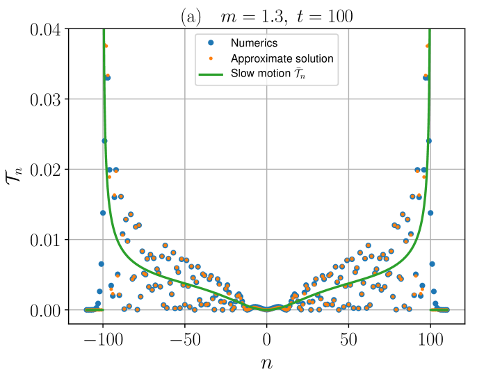
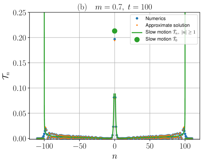
Figure 5: Comparing the approximate solution for $\mathcal{T}_{n}$ in the form of Eq. (10.1), the corresponding solution (3.20) for the kinetic temperatures wherein ${\mathcal{V}}_{n}$ are found numerically, and the slow motion $\bar{\mathcal{T}}_{n}$. (a) The case of a heavy defect, (b) the case of a light defect (here $\bar{\mathcal{T}}_{n}$ is represented as a continuum quantity for $|n|\geq 1$)

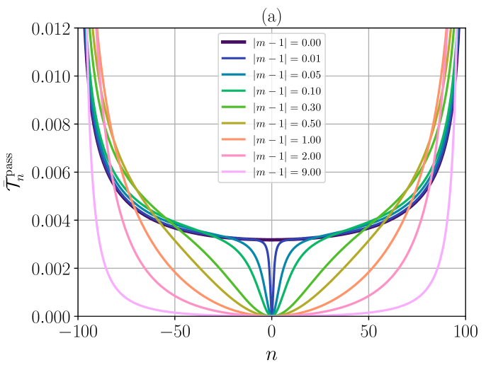
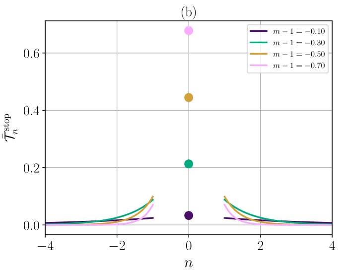
Figure 6: The components of the slow thermal motion $\bar{\mathcal{T}}_{n}$ for various mass of isotopic defect $m$. (a) $\bar{\mathcal{T}}_{n}^{\mathrm{pass}}$ given by Eq. (10.4), (b) $\bar{\mathcal{T}}_{n}^{\mathrm{stop}}$ given by Eq. (10.11)

11 Conclusion

In the paper we have applied the asymptotic technique based on the method of stationary phase and have obtained the approximate large-time description of the thermal motion caused by a source on an isotopic defect in a 1D harmonic crystal. The most important new results of the paper are formulae (10.3), (10.4), (10.5), which provide continualization and asymptotic uncoupling of the propagating outside the defect component of the thermal motion into the superposition of the slow and fast motions. The slow motion is related with ballistic heat transport, whereas the fast motion is energy oscillation related with the transformation of the kinetic energy into the potential one and in the opposite direction.

In the case of a heavy defect the thermal motion can be described by the propagating part only, and both slow and fast components are zero at the defect, see Fig. 5(a). We suggest calling this phenomenon “anti-localization”. The physical meaning of the anti-localization is a tendency for the unsteady propagating wave-field to avoid a neighbourhood of a defect. In the paper we first time demonstrate how the anti-localization influences on the propagating wave-field. Namely, one can observe that the greater the quantity $|m-1|$ (the dimensionless difference between the mass of the defect and mass of any other particle), the wider the anti-localization zone near the defect, and more energy concentrates closer to the leading wave-front $|n|=t$, see Fig. 6(a). For the best of our knowledge, the anti-localization was never treated as a general phenomenon. But its existence under certain, still unknown, conditions is in an excellent agreement both with our results and observations in studies Rubin_1963 ; Takizawa1968 ; kaplunov1986torsional ; Mueller1962 ; Kashiwamura1962 ; Gendelman2021 concerning the same or different dispersive systems with inclusions or defects.

In the case of a light defect the slow motion is the superposition of anti-localized propagating and localized components. Localized component is a non-vanishing undamped oscillation, which traps some portion of the full energy and conserves it forever. The most complete description of the localized component is obtained by Rubin in Rubin_1963 and has been discussed in the current paper by means of a different approach.

To obtain the vanishing propagating component of the fast and slow motion we have estimated the exact solution in the integral form at a moving point of observation. This approach allows one to describe running waves, wave-fronts, and to describe the wave-field as a whole. Thus, the obtained solution is valid in a wide range of a spatial co-ordinate (i.e., a particle number), everywhere excepting a neighbourhood of the leading wavefront. In previous studies only particular results were obtained, which characterize the solution at some points and for particular values for the mass of the defect (see Remark 7). Formula (7.59) describing the fundamental solution for particle velocity at the leading wavefront, for the best of our knowledge, is also new. All our results have been verified numerically, and a good agreement for the case $m\not\simeq 1$ has been demonstrated. On the other hand, all our results (as well as the previous ones) become practically inapplicable for small $n$ at the case $m\simeq 1$, $m\neq 1$ (see Sect. 9). To analyse this case it is necessary to construct a uniform asymptotics, which takes into account the singularities collocations.

Finally, let us discuss how the results of the paper can be generalized, and how one can use them in physical applications. In our opinion, the same approach can be applied to various more complicated non-uniform systems (discrete or continuum ones) with a single point inclusion or a defect. The derivation of the expression for the slow motion describing heat transfer in a polyatomic harmonic lattice with an isotopic defect (in particular, in a graphene lattice) could be a possible direction of the future work. The method also can be applied to the problem where the source is located outside the defect particle. Besides, we expect that the solution describing the slow motion for the problem concerning ballistic heat transport in the same system with suddenly applied point heat source of a constant intensity Gavrilov2022cmat ; Gavrilov2019cmat ; Gavrilov2020cmat can be obtained by time integration of the slow motion found in this paper. In our opinion, the results of the paper and such a future work can allow us to improve the existing theoretical models for ballistic thermal transport in isotopically modified graphene Chen2012 .

Another important application of the approach proposed in this paper is related with the possibility to suggest simple analytical description of non-stationary Kapitza thermal resistance, basing on the model proposed in Paul2020 ; Gendelman2021 .

Appendix A Non-dimensionalization

The equations of motion for the system under consideration are

$$\tilde{m}_{n}\frac{\mathrm{d}^{2}{\tilde{u}}_{n}}{\mathrm{d}\tilde{t}^{2}}-\tilde{C}(\tilde{u}_{n+1}-2\tilde{u}_{n}+\tilde{u}_{n-1})=\delta_{n}\tilde{p}\big{(}\tilde{t}\big{)}.$$ (A.1)

Here $n\in\mathbb{Z}$, $\tilde{t}$ is the time, $\tilde{u}_{n}(\tilde{t})$ is the displacement of the particle with a number $n$, $\tilde{m}_{n}$ is the mass of a particle with number $n$:

$$\tilde{m}_{n}=\tilde{M}+\delta_{n}(\tilde{m}-\tilde{M}),$$ (A.2)

$\tilde{C}$ is the bond stiffness. The dimensionless equations of motion (3.1) can be obtained by introducing the following dimensionless quantities:

$$u_{n}=\frac{\tilde{u}_{n}}{\tilde{A}};\quad t=\omega\tilde{t};\quad p=\frac{\tilde{p}}{\tilde{C}\tilde{A}},\quad m=m_{0}=\frac{\tilde{m}}{\tilde{M}}.$$ (A.3)

Here $\tilde{A}$ is the lattice constant (the distance between neighbouring particles); $\omega\stackrel{{\scriptstyle\mbox{\scriptsize def}}}{{=}}\sqrt{{\tilde{C}}/{\tilde{M}}}$.

Appendix B The Erdélyi lemma

Theorem B.1

Let $a>0,\ \alpha\geq 1,\ \beta>0$, $f(\Omega)\in C^{\infty}$, $f^{(n)}(a)=0\ \forall n.$ Then

$$\int_{0}^{a}\Omega^{\beta-1}f(\Omega)\,\mathrm{e}^{\mathrm{i}t\Omega^{\alpha}}\,\mathrm{d}\Omega\sim\sum_{k=0}^{\infty}c_{k}t^{-\frac{k+\beta}{\alpha}},\quad t\to\infty;$$ (B.1)

$$c_{k}=\frac{f^{(k)}(0)}{k!\alpha}\,\Gamma\left(\frac{k+\beta}{\alpha}\right)\mathrm{e}^{\frac{\mathrm{i}\pi(k+\beta)}{2\alpha}}.$$ (B.2)

The proof can be found in erdelyi1956asymptotic ; Fedoryuk1977 .

In Sect. 7 we sometimes apply Erdélyi lemma to integrals, where $\beta=1$, $0<\alpha<1$. The corresponding asymptotics can be obtained by taking $\Omega^{\alpha}$ as the new integration variable, and applying the Erdélyi lemma to the obtained integral.

Appendix C The trapped energy ratio

According to Eq. (3.17) the initial kinetic energy, as well as the total energy of the chain for all $t$, is $\mathcal{E}$. On the other hand, according to (3.14), (3.19)

$$\langle K_{n}\rangle=\frac{1}{2}{\mathcal{E}}\mathcal{T}_{n}.$$ (C.1)

One has

$$\frac{\sum_{n=-\infty}^{\infty}\langle K_{n}(t)\rangle}{\mathcal{E}}=\frac{\sum_{n=-\infty}^{\infty}\mathcal{T}_{n}(t)}{2}.$$ (C.2)

Considering the energy trapped near the defect as $t\to\infty$, we substitute into Eq. (C.2) $\mathcal{T}_{n}=\mathcal{T}_{n}^{\mathrm{stop}}\simeq 2mm_{n}({v}_{n}^{\mathrm{stop}})^{2}$:

$$\frac{\sum_{n=-\infty}^{\infty}\langle K_{n}(t)\rangle}{\mathcal{E}}=m\sum_{n=-\infty}^{\infty}m_{n}({v}_{n}^{\mathrm{stop}})^{2}=m^{2}(v_{0}^{\mathrm{stop}})^{2}+2m\sum_{n=1}^{\infty}({v}_{n}^{\mathrm{stop}})^{2}.$$ (C.3)

Using Eq. (10.9) to calculate the right-hand side of (C.3) at $t=\frac{\pi k}{\Omega_{0}}$, $k\in\mathbb{Z}$, $k\to\infty$ (when the trapped kinetic energy equals the trapped total energy), we obtain the ratio $R$ of the trapped total energy to the total energy of the chain. Due to (10.9) on has

$$({v}^{\mathrm{stop}}_{n})^{2}\Big{|}_{t=\frac{\pi k}{\Omega_{0}}}=\frac{4(1-m)^{2}m^{2(|n|-1)}}{(2-m)^{2(|n|+1)}}.$$ (C.4)

Calculating the sum of the geometric series in the right-hand side of Eq. (C.3), one, finally, gets

$$R=\frac{4(1-m)^{2}}{m(2-m)^{2}}\left(m+\frac{2q}{1-q}\right)=1-\frac{m}{2-m}.$$ (C.5)

Here

$$q=\frac{m^{2}}{(2-m)^{2}}$$ (C.6)

is a common ratio for the geometric series.

The plot of the trapped total energy $R$ versus $m$ is presented in Fig. 7. For $m\to+0$ all energy is trapped near the defect, for $m\to 1-0$ all energy is radiated away from the defect.

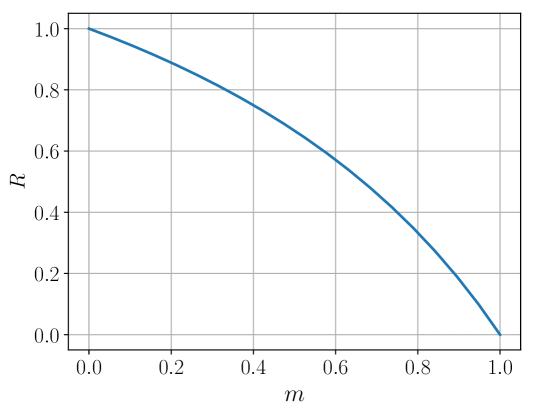
Figure 7: The trapped total energy ratio $R$ versus $m$

Formula (C.5) was previously obtained in Rubin_1963 .

References

- (1) Hamilton, W.R.: Propagation of motion in elastic medium — discrete molecules (1839). In: A. Conway, A. McConnell (eds.) The Mathematical Papers of Sir William Rowan Hamilton, Vol. II: Dynamics, pp. 527–575. Cambridge at the Univesity Press (1940)
- (2) Havelock, T.H.: On the instantaneous propagation of disturbance in a dispersive medium. Philosophical Magazine 19(109), 160–168 (1910). https://doi.org/10.1080/14786440108636785
- (3) Schrödinger, E.: Zur Dynamik elastisch gekoppelter Punktsysteme. Annalen der Physik 349(14), 916–934 (1914). https://doi.org/10.1002/andp.19143491405
- (4) Mühlich, U., Abali, B.E., dell’Isola, F.: Commented translation of Erwin Schrödinger’s paper ‘On the dynamics of elastically coupled point systems’ (Zur Dynamik elastisch gekoppelter Punktsysteme). Mathematics and Mechanics of Solids 26(1), 133–147 (2020). https://doi.org/10.1177/1081286520942955
- (5) Klein, G., Prigogine, I.: Sur la mecanique statistique des phenomenes irreversibles III. Physica 19(1-12), 1053–1071 (1953). https://doi.org/10.1016/S0031-8914(53)80120-5
- (6) Hemmer, P.C.: Dynamic and stochastic types of motion in the linear chain. Ph.D. thesis, Norges tekniske høgskole, Trondheim (1959)
- (7) Rieder, Z., Lebowitz, J.L., Lieb, E.: Properties of a harmonic crystal in a stationary nonequilibrium state. Journal of Mathematical Physics 8(5), 1073–1078 (1967). https://doi.org/10.1063/1.1705319
- (8) Lepri, S., Livi, R., Politi, A.: Thermal conduction in classical low-dimensional lattices. Physics reports 377(1), 1–80 (2003). https://doi.org/10.1016/S0370-1573(02)00558-6
- (9) Chang, C.W., Okawa, D., Garcia, H., Majumdar, A., Zettl, A.: Breakdown of Fourier’s law in nanotube thermal conductors. Physical review letters 101(7), 075,903 (2008). https://doi.org/10.1103/PhysRevLett.101.075903
- (10) Hsiao, T.K., Huang, B.W., Chang, H.K., Liou, S.C., Chu, M.W., Lee, S.C., Chang, C.W.: Micron-scale ballistic thermal conduction and suppressed thermal conductivity in heterogeneously interfaced nanowires. Physical Review B 91(3), 035,406 (2015). https://doi.org/10.1103/PhysRevB.91.035406
- (11) Hsiao, T.K., Chang, H.K., Liou, S.C., Chu, M.W., Lee, S.C., Chang, C.W.: Observation of room-temperature ballistic thermal conduction persisting over 8.3 m in SiGe nanowires. Nature nanotechnology 8(7), 534–538 (2013). https://doi.org/10.1038/nnano.2013.121
- (12) Bae, M.H., Li, Z., Aksamija, Z., Martin, P.N., Xiong, F., Ong, Z.Y., Knezevic, I., Pop, E.: Ballistic to diffusive crossover of heat flow in graphene ribbons. Nature Communications 4(1), 1734 (2013). https://doi.org/10.1038/ncomms2755
- (13) Saito, R., Mizuno, M., Dresselhaus, M.S.: Ballistic and diffusive thermal conductivity of graphene. Physical Review Applied 9(2), 024,017 (2018). https://doi.org/10.1103/PhysRevApplied.9.024017
- (14) Xu, X., Pereira, L.F.C., Wang, Yu., Wu, J., Zhang, K., Zhao, X., Bae, S., Tinh, B., Xie, R., Thong, J.T.L., Hong, B.H., Loh, K.P., Donadio, D., Li, B., Özyilmaz, B.: Length-dependent thermal conductivity in suspended single-layer graphene. Nature Communications 5(1), 3689 (2014). https://doi.org/10.1038/ncomms4689
- (15) Krivtsov, A.M.: Energy oscillations in a one-dimensional crystal. Doklady Physics 59(9), 427–430 (2014). https://doi.org/10.1134/S1028335814090080
- (16) Krivtsov, A.M.: Heat transfer in infinite harmonic one-dimensional crystals. Doklady Physics 60(9), 407–411 (2015). https://doi.org/10.1134/S1028335815090062
- (17) Kuzkin, V.A., Krivtsov, A.M.: Fast and slow thermal processes in harmonic scalar lattices. Journal of Physics: Condensed Matter 29(50), 505,401 (2017). https://doi.org/10.1088/1361-648X/aa98eb
- (18) Krivtsov, A.M.: The ballistic heat equation for a one-dimensional harmonic crystal. In: H. Altenbach, et al. (eds.) Dynamical Processes in Generalized Continua and Structures, Advanced Structured Materials 103, pp. 345–358. Springer (2019). https://doi.org/10.1007/978-3-030-11665-1_19
- (19) Gavrilov, S.N., Krivtsov, A.M., Tsvetkov, D.V.: Heat transfer in a one-dimensional harmonic crystal in a viscous environment subjected to an external heat supply. Continuum Mechanics and Thermodynamics 31, 255–272 (2019). https://doi.org/10.1007/s00161-018-0681-3
- (20) Gavrilov, S.N., Krivtsov, A.M.: Thermal equilibration in a one-dimensional damped harmonic crystal. Physical Review E 100(2), 022,117 (2019). https://doi.org/10.1103/PhysRevE.100.022117
- (21) Kuzkin, V.A.: Thermal equilibration in infinite harmonic crystals. Continuum Mechanics and Thermodynamics 31(5), 1401–1423 (2019). https://doi.org/10.1007/s00161-019-00758-2
- (22) Sokolov, A.A., Müller, W.H., Porubov, A.V., Gavrilov, S.N.: Heat conduction in 1D harmonic crystal: Discrete and continuum approaches. International Journal of Heat and Mass Transfer 176, 121,442 (2021). https://doi.org/10.1016/j.ijheatmasstransfer.2021.121442
- (23) Kuzkin, V.A.: Unsteady ballistic heat transport in harmonic crystals with polyatomic unit cell. Continuum Mechanics and Thermodynamics 31(6), 1573–1599 (2019). https://doi.org/10.1007/s00161-019-00802-1
- (24) Gavrilov, S.N., Krivtsov, A.M.: Steady-state ballistic thermal transport associated with transversal motions in a damped graphene lattice subjected to a point heat source. Continuum Mechanics and Thermodynamics 34(1), 297–319 (2022). https://doi.org/10.1007/s00161-021-01059-3
- (25) Panchenko, A.Yu., Kuzkin, V.A., Berinskii, I.E.: Unsteady ballistic heat transport in two-dimensional harmonic graphene lattice. Journal of Physics: Condensed Matter 34(16), 165,402 (2022). https://doi.org/10.1088/1361-648X/ac5197
- (26) Gavrilov, S.N.: Discrete and continuum fundamental solutions describing heat conduction in a 1D harmonic crystal: Discrete-to-continuum limit and slow-and-fast motions decoupling. International Journal of Heat and Mass Transfer 194, 123,019 (2022). https://doi.org/10.1016/j.ijheatmasstransfer.2022.123019
- (27) Slepyan, L.I.: Nestatsionarnye uprugie volny [Non-stationary elastic waves]. Sudostroenie [Shipbuilding], Leningrad (1972). In Russian
- (28) Montroll, E.W., Potts, R.B.: Effect of defects on lattice vibrations. Physical Review 100(2), 525–543 (1955). https://doi.org/10.1103/PhysRev.100.525
- (29) Indeitsev, D.A., Kuznetsov, N.G., Motygin, O.V., Mochalova, Yu.A.: Lokalizatsia lineynykh voln [Localization of linear waves]. Izdatelstvo Sankt-Peterburgskogo universiteta [St. Petersburg University publishing house], St. Petersburg (2007). (in Russian)
- (30) Andrianov, I.V., Danishevs’kyy, V.V., Kalamkarov, A.L.: Vibration localization in one-dimensional linear and nonlinear lattices: discrete and continuum models. Nonlinear Dynamics 72, 37–48 (2012). https://doi.org/10.1007/s11071-012-0688-4
- (31) Gavrilov, S.N., Shishkina, E.V., Mochalova, Yu.A.: Non-stationary localized oscillations of an infinite string, with time-varying tension, lying on the Winkler foundation with a point elastic inhomogeneity. Nonlinear Dynamics 95(4), 2995–3004 (2019). https://doi.org/10.1007/s11071-018-04735-3
- (32) Mishuris, G.S., Movchan, A.B., Slepyan, L.I.: Localized waves at a line of dynamic inhomogeneities: General considerations and some specific problems. Journal of the Mechanics and Physics of Solids 138, 103,901 (2020). https://doi.org/10.1016/j.jmps.2020.103901
- (33) Teramoto, E., Takeno, S.: Time dependent problems of the localized lattice vibration. Progress of Theoretical Physics 24(6), 1349–1368 (1960). https://doi.org/10.1143/PTP.24.1349
- (34) Kashiwamura, S.: Statistical dynamical behaviors of a one-dimensional lattice with an isotopic impurity. Progress of Theoretical Physics 27(3), 571–588 (1962). https://doi.org/10.1143/PTP.27.571
- (35) Magalinskii, V.B.: Dynamical model in the theory of the brownian motion. Soviet Physics JETP-USSR 9(6), 1381–1382 (1959)
- (36) Müller, I.: Durch eine äußere Kraft erzwungene Bewegung der mittleren Masse eineslinearen Systems von durch federn verbundenen Massen [The forced motion of the sentral mass in a linear mass-spring chain of n masses under the action of an external force]. Diploma thesis, Technical University Aachen (1962)
- (37) Müller, I., Weiss, W.: Thermodynamics of irreversible processes — past and present. The European Physical Journal H 37(2), 139–236 (2012). https://doi.org/10.1140/epjh/e2012-20029-1
- (38) Turner, R.E.: Motion of a heavy particle in a one dimensional chain. Physica 26(4), 269–273 (1960). https://doi.org/10.1016/0031-8914(60)90022-7
- (39) Rubin, R.J.: Statistical dynamics of simple cubic lattices. Model for the study of brownian motion. Journal of Mathematical Physics 1(4), 309–318 (1960). https://doi.org/10.1063/1.1703664
- (40) Rubin, R.J.: Statistical dynamics of simple cubic lattices. Model for the study of brownian motion. II. Journal of Mathematical Physics 2(3), 373–386 (1961). https://doi.org/10.1063/1.1703723
- (41) Rubin, R.J.: Momentum autocorrelation functions and energy transport in harmonic crystals containing isotopic defects. Physical Review 131(3), 964–989 (1963). https://doi.org/10.1103/PhysRev.131.964
- (42) Takizawa, E.I., Kobayasi, K.: Localized vibrations in a system of coupled harmonic oscillators. Chinese Journal of Physics 5(1), 11–17 (1968)
- (43) Takizawa, E.I., Kobayasi, K.: On the stochastic types of motion in a system oflinear harmonic oscillators. Chinese Journal of Physics 6(1), 39–66 (1968)
- (44) Lee, M.H., Florencio, J., Hong, J.: Dynamic equivalence of a two-dimensional quantum electron gas and a classical harmonic oscillator chain with an impurity mass. Journal of Physics A 22(8), L331–L335 (1989). https://doi.org/10.1088/0305-4470/22/8/005
- (45) Yu, M.B.: Momentum autocorrelation function of an impurity in a classical oscillator chain with alternating masses — I. General theory. Physica A 398, 252–263 (2014). https://doi.org/10.1016/j.physa.2013.11.023
- (46) Yu, M.B.: Momentum autocorrelation function of an impurity in a classical oscillator chain with alternating masses II. Illustrations. Physica A 438, 469–486 (2015). https://doi.org/10.1016/j.physa.2015.06.014
- (47) Yu, M.B.: Momentum autocorrelation function of an impurity in a classical oscillator chain with alternating masses III. Some limiting cases. Physica A 447, 411–421 (2016). https://doi.org/10.1016/j.physa.2015.12.034
- (48) Yu, M.B.: A monatomic chain with an impurity in mass and Hooke constant. The European Physical Journal B 92, 272 (2019). https://doi.org/10.1140/epjb/e2019-100383-1
- (49) Kannan, V.: Heat conduction in low dimensional lattice systems. Ph.D. thesis, Rutgers the State University of New Jersey – New Brunswick (2013)
- (50) Paul, J., Gendelman, O.V.: Kapitza resistance in basic chain models with isolated defects. Physics Letters A 384(10), 126,220 (2020). https://doi.org/10.1016/j.physleta.2019.126220
- (51) Gendelman, O.V., Paul, J.: Kapitza thermal resistance in linear and nonlinear chain models: Isotopic defect. Physical Review E 103(5), 052,113 (2021). https://doi.org/10.1103/PhysRevE.103.052113
- (52) Plyukhin, A.V.: Non-Clausius heat transfer: the example of harmonic chain with an impurity. Journal of Statistical Mechanics: Theory and Experiment 2020(6), 063,212 (2020). https://doi.org/10.1088/1742-5468/ab837c
- (53) Chen, S., Wu, Q., Mishra, C., Kang, J., Zhang, H., Cho, K., Cai, W., Balandin, A.A., Ruoff, R.S.: Thermal conductivity of isotopically modified graphene. Nature Materials 11(3), 203–207 (2012). https://doi.org/10.1038/nmat3207
- (54) Vladimirov, V.S.: Equations of Mathematical Physics. Marcel Dekker, New York (1971)
- (55) Slepyan, L.I., Tsareva, O.V.: Energy flux for zero group velocity of the carrier wave. Soviet Physics Doklady 32, 522–526 (1987)
- (56) Ayzenberg-Stepanenko, M.V., Slepyan, L.I.: Resonant-frequency primitive waveforms and star waves in lattices. Journal of Sound and Vibration 313(3), 812–821 (2008). https://doi.org/10.1016/j.jsv.2007.11.047
- (57) Abdukadirov, S.A., Ayzenberg-Stepanenko, M.V., Osharovich, G.G.: Resonant waves and localization phenomena in lattices. Philosophical Transactions of the Royal Society A: Mathematical, Physical and Engineering Sciences 377(2156), 20190,110 (2019). https://doi.org/10.1098/rsta.2019.0110
- (58) Erdélyi, A.: Asymptotic expansions. Dover Publications, New York (1956)
- (59) Fedoryuk, M.V.: Metod perevala [The Saddle-Point Method]. Nauka [Science], Moscow (1977). In Russian
- (60) Temme, N.M.: Asymptotic Methods for Integrals. World Scientific (2014). https://doi.org/10.1142/9195
- (61) van der Corput, J.G.: On the method of critical points. i. K. Ned. Akad. Wet. Indag. Math. 10, 201–209 (1948)
- (62) Gavrilov, S.: Non-stationary problems in dynamics of a string on an elastic foundation subjected to a moving load. Journal of Sound and Vibration 222(3), 345–361 (1999). https://doi.org/10.1006/jsvi.1998.2051
- (63) Olver, F.: Asymptotics and Special Functions. A.K. Peters/CRC Press, New York (1997). https://doi.org/10.1201/9781439864548
- (64) Kaplunov, Yu.D.: Torsional vibrations of a rod on a deformable base under a moving inertial load. Mechanics of solids 21(6), 167–170 (1986)
- (65) Allen, P.B., Nghiem, N.A.: Heat pulse propagation and nonlocal phonon heat transport in one-dimensional harmonic chains. Physical Review B 105(17), 174,302 (2022). https://doi.org/10.1103/PhysRevB.105.174302
- (66) Gavrilov, S.N., Krivtsov, A.M.: Steady-state kinetic temperature distribution in a two-dimensional square harmonic scalar lattice lying in a viscous environment and subjected to a point heat source. Continuum Mechanics and Thermodynamics 32(1), 41–61 (2020). https://doi.org/10.1007/s00161-019-00782-2