Generalized Leverage Scores: Geometric Interpretation and Applications

Abstract

In problems involving matrix computations, the concept of leverage has found a large number of applications. In particular, leverage scores, which relate the columns of a matrix to the subspaces spanned by its leading singular vectors, are helpful in revealing column subsets to approximately factorize a matrix with quality guarantees. As such, they provide a solid foundation for a variety of machine-learning methods. In this paper we extend the definition of leverage scores to relate the columns of a matrix to arbitrary subsets of singular vectors. We establish a precise connection between column and singular-vector subsets, by relating the concepts of leverage scores and principal angles between subspaces. We employ this result to design approximation algorithms with provable guarantees for two well-known problems: generalized column subset selection and sparse canonical correlation analysis. We run numerical experiments to provide further insight on the proposed methods. The novel bounds we derive improve our understanding of fundamental concepts in matrix approximations. In addition, our insights may serve as building blocks for further contributions.

algorithm

1 Introduction

When dealing with data in matrix form, it is often useful to find compact low-dimensional approximations. One way to find such an approximation is by computing a singular value decomposition (SVD), which offers a representation of a matrix in terms of a set of linearly-independent factors, conveniently sorted in order of importance. The SVD is optimal the following sense: for any constant $k$, it reveals the best rank-$k$ approximation of a matrix, as measured by a family of matrix norms.

A drawback of SVD is that the resulting factors do not correspond directly to the rows or columns of the input matrix and lack an intuitive interpretation. To address this issue, many works in the literature seek approximate factorizations in terms of elements of the matrix: instead of settling for a set of abstract factors, like those offered by the SVD, we aim to find a subset of rows or columns that are particularly representative of the whole matrix.

Computing an SVD is a tractable problem and has been the subject of extensive research. Thus, efficient methods exist to obtain an SVD to any desired level of precision (Golub & Van Loan, 1996). When we wish to select a subset of matrix elements instead, the task often becomes computationally hard under various natural objectives (Civril, 2014; Shitov, 2017). Therefore, research in this area has focused on finding efficient approximation algorithms.

An example of a more intuitive matrix approximation is the column subset selection problem (Deshpande et al., 2006; Boutsidis et al., 2009), which, given a matrix and a number $k$, asks for the $k$ best columns, in the following sense:

Problem 1.

Column subset selection (CSS). Given a matrix $A\in\mathbb{R}^{m\times n}$ and a positive integer $k$ smaller than the rank of $A$, find a matrix $C$ comprised of $k$ columns of $A$ to minimize

$$\|A-CC^{+}A\|_{F}^{2},$$ (1)

where $C^{+}$ is the Moore-Penrose pseudoinverse of $C$.

The matrix $CC^{+}A$ is the best Frobenius-norm approximation of $A$ in the column-space of $C$ and is efficiently computable. It is easy to verify that the problem of maximizing $\|CC^{+}A\|_{F}^{2}$ is equivalent to Problem 1, meaning that the set of optimal solutions remain the same.

Leverage scores and good column subsets. In finding good column subsets for the CSS problem, leverage scores have proved very useful. These scores — to be precisely defined later — relate the columns of a matrix to the subspace spanned by its top singular vectors. Thus, they might reveal whether a column subset is particularly representative. Leverage scores, and variants thereof, have been employed to design approximation algorithms for CSS and related problems (Drineas et al., 2006b, 2008; Mahoney & Drineas, 2009; Boutsidis et al., 2009; Papailiopoulos et al., 2014). We give a more detailed overview of related work in the appendix. Leverage scores can be traced back to the concept of statistical leverage, long employed in statistics and the analysis of linear regression (Chatterjee & Hadi, 1986).

The techniques based on leverage scores, however, do not apply to other matrix-approximation problems, such as the following generalization of CSS (in maximization form):

Problem 2.

Generalized column subset selection (GCSS). Given two matrices $A\in\mathbb{R}^{m\times n}$, $B\in\mathbb{R}^{m\times p}$ and a positive integer $k$ smaller than the rank of $A$, find a matrix $C$ comprised of $k$ columns of $A$ to maximize

$$\|CC^{+}B\|_{F}^{2}.$$ (2)

The reason that leverage scores are no longer helpful is that they relate the columns of $A$ to its top-$k$ singular vectors, and these, in turn, may not provide a good approximation of $B$. The following question arises naturally: is there useful information elsewhere among the singular subspaces of $A$?

We will show that, indeed, such information can be drawn from subspaces spanned by arbitrary sets of singular vectors. This information, in the form of leverage scores, will be useful to tackle problems like GCSS.

1.1 Our Contributions.

In this paper we introduce the concept of generalized leverage scores, which relate the columns of a matrix to the subspace spanned by an arbitrary subset of its singular vectors. Our definition, which provides a natural extension of leverage scores, can be employed to obtain approximation algorithms for a variety of problems. Furthermore, the analysis leading to these algorithms yields insightful results of independent interest, relating leverage scores and the concept of angles between subspaces. In more detail, we make the following contributions.

Generalized leverage scores and connections to principal angles: We introduce the concept of generalized leverage scores, defined in terms of an arbitrary set of singular vectors, as contrasted to the standard leverage scores, which are defined with respect to the leading singular vectors. We show how this generalization enables the application of leverage-score-based techniques to a new array of problems, leading to algorithms with approximation guarantees.

The cornerstone of these results is a novel inequality that gives a geometric interpretation of the generalized leverage scores, by relating them to the principal angles between matrix columns and singular vectors. The special case of standard leverage scores, which is of independent interest, will be treated separately and proved using different arguments. We believe that our results, which relate two fundamental quantities, solidify our understanding of how leverage scores connect matrix columns and singular vectors.

Applications: We showcase the applicability of the generalized leverage scores by providing approximation algorithms for two well-known problems:

For GCSS (Problem 2), we show that choosing singular vectors and generalized leverage scores to cover a $(1-\epsilon)$-factor of readily accessible quantities, we find a column submatrix $C$ of $A$ such that $\|CC^{+}B\|_{F}^{2}\geq(1-\epsilon)^{2}\|B\|_{F}^{2}$. This is akin to a known result for CSS (Papailiopoulos et al., 2014), and complementary to the only other known bound — to our knowledge — for GCSS (Bhaskara et al., 2016). In contrast to the result of Bhaskara et al. (2016), the number of columns chosen by our algorithm does not depend on the smallest singular value of the optimal subset, which is unknown. Instead, it depends on the decay of the generalized leverage scores, which is trivially computable. In particular, if the scores follow a power-law decay, $\mathcal{O}\!\left(\frac{\sigma_{\omega}^{2}k}{\sigma_{\mu}^{2}\epsilon}\right)$ columns suffice, where $\sigma_{\omega},\sigma_{\mu}$ are a choice of singular values that depends on the approximation constant $\epsilon$ — the user, thus, has control over this ratio.

For sparse canonical correlation analysis (SparseCCA) (Hardoon & Shawe-Taylor, 2011; Uurtio et al., 2017) we give similar results (see Section 5.2). Given input matrices $A$ and $B$, we use a similar criterion as before to find column subsets of both matrices whose canonical correlations add up to a $(1-\epsilon)^{4}$ factor of the total canonical correlations between $A$ and $B$. We are not aware of other algorithms that give guarantees for SparseCCA in these terms.

The cost of the proposed algorithms is dominated by the task of finding an SVD. Thus, our approaches can take full advantage of the plethora of existing techniques for this purpose, as well as fast approximate methods.

2 Preliminaries

We will use upper and lowercase letters for matrices and vectors, respectively, as in $A$ and $x$. We will also use uppercase letters for sets. Context will be sufficient to tell sets and matrices apart. For a matrix $A$ we write $A_{i,:}$ to denote its $i$-th row. We write $A^{+}$ to denote the pseudoinverse of $A$.

As in other works involving leverage scores, the singular value decomposition will make frequent appearances in this paper. We use the subindex $k$, as in $U_{k}$ and $V_{k}$, to denote the “truncated” submatrices of a singular value decomposition, obtained by retaining the first $k$ singular vectors only. Analogously, given a set $R$ of natural numbers, $U_{R}$ and $V_{R}$ will denote the matrices obtained by retaining the singular vectors indexed by $R$. For instance, note that $U_{k}=U_{\{1,\dots,k\}}$.

Chief among our cast of characters are the leverage scores.

Definition 2.1.

Given a matrix $A$ with singular value decomposition $A=U\Sigma V^{T}$, the rank-$k$ leverage score of the $i$-th column of $A$ is defined as $\|(V_{k})_{i,:}\|_{2}^{2}$.

Given a matrix $A$, we will denote the $i$-th diagonal element of $AA^{+}$ as $\ell_{i}(A)$. This quantity is sometimes known in the statistics literature as statistical leverage of the $i$-th row of $A$, and as we will see, it is connected to the leverage scores. Even though this choice of nomenclature may occasionally lead to confusion, we retain it for historical reasons. We ask the reader to remark the distinction in this text between statistical leverages and leverage scores.

Also relevant is the concept of principal angles between subspaces, defined as follows (Björck & Golub, 1973):

Definition 2.2.

Let $F$ and $G$ be subspaces of $\mathbb{R}^{n}$. Let the columns of matrices $Q$ and $T$ be orthonormal bases of $F$ and $G$, respectively. The principal angles between $F$ and $G$ are the angles whose cosines are the singular values of $Q^{T}T$.

We will often speak of angles between two matrices to mean the angles between the subspaces spanned by their columns.

We make use of projection matrices and their properties.

Definition 2.3.

A matrix $H$ is said to be a projection matrix (or projector) if $H^{2}=H$.

For any projection matrix $H$, we have:

Property 1.

$\sum_{j}H_{ij}^{2}=H_{ii}$.

Property 2.

$H$ is invariant with respect to the basis of the space onto which it projects.

Property 3.

$tr(H)=r$, where $r$ is the dimension of the space onto which $H$ projects.

3 Leverage Scores and the Top-$k$ Singular Subspace

In this section we present our first result, which relates the two fundamental quantities defined in the previous section: the leverage scores and the principal angles between subspaces. Even though this is a special case of the result in Section 4, we treat it separately for two reasons: first, it is of independent interest and, to the best of our knowledge, novel; second, the proof techniques will be useful — but insufficient — for the more general results of Section 4, so this case serves as a natural, more accessible, preamble.

To state our result, we will rely on two easily verified facts, given below. Here, we consider matrices $A=U\Sigma V^{T}$ and $C=AS$, where $S$ is a column selection matrix (binary matrix with unit-norm columns), and thus $C$ is comprised of a column subset of $A$.

Fact 1.

The sum of the leverage scores of the columns of $C=AS$ is equal to $\|V_{k}^{T}S\|_{F}^{2}$.

Fact 2.

The sum of the squared cosines of the principal angles between $C$ and $U_{k}$ is equal to $\|CC^{+}U_{k}\|_{F}^{2}$.

To verify Fact 2, note that if $U_{C}$ is an orthonormal basis for $C$, then $\|U_{C}^{T}U_{k}\|_{F}^{2}=\|U_{C}U_{C}^{T}U_{k}\|_{F}^{2}=\|U_{C}U_{C}^{+}U_{k}\|_{F}^{2}=\|CC^{+}U_{k}\|_{F}^{2}$. The last equality relies on Property 2.

We now state the main result of this section.

Theorem 3.1.

Consider a matrix $A\in\mathbb{R}^{m\times n}$ and its singular value decomposition $A=U\Sigma V^{T}$. Consider a column sampling matrix $S\in\mathbb{R}^{n\times r}$ and write $C=AS$. Then

$$\|CC^{+}U_{k}\|_{F}^{2}\geq\|V_{k}^{T}S\|_{F}^{2}.$$

In words, the sum of the leverage scores of a column subset provides a lower bound for the sum of the cosines of the principal angles between two subspaces: the one spanned by said column subset and the one spanned by the top-$k$ left singular vectors. We believe this result provides new insight on how the leverage scores connect column subsets and the top-$k$ singular vectors.

In our proof of Theorem 3.1 we will make use of the following technical result, which characterizes the change in the statistical leverages of a matrix upon multiplication of its rows by scalars. Recall that $\ell_{i}(A)$ is the $i$-th diagonal element of $AA^{+}$.

Lemma 3.2.

Consider a matrix $X\in\mathbb{R}^{n\times k}$ of rank $k$. Additionally, consider a non-negative real number $\alpha$ and a diagonal matrix ${\tilde{\Sigma}^{(i)}}$ defined as follows: ${\tilde{\Sigma}^{(i)}}_{ii}=\alpha$, ${\tilde{\Sigma}^{(i)}}_{jj}=1$ for all $j\neq i$. We write $x_{j}=X_{j,:}^{T}$, for any $j$. Then

$$\ell_{j}({\tilde{\Sigma}^{(i)}}X)=\ell_{j}(X)-\frac{(\alpha^{2}-1)(x_{j}^{T}(X^{T}X)^{-1}x_{i})^{2}}{1+(\alpha^{2}-1)\ell_{i}(X)},$$

and in particular,

$$\ell_{i}({\tilde{\Sigma}^{(i)}}X)=\frac{\alpha^{2}\ell_{i}(X)}{1+(\alpha^{2}-1)\ell_{i}(X)}.$$

Proof. First, observe that since $X$ is full column rank, $XX^{+}=X(X^{T}X)^{-1}X^{T}$. Note also that scaling one row of $X$ through multiplication by a scalar is a rank-1 update of $X$. In particular, let $x_{i}^{T}$ be the $i$-th row of $X$, and consider the product $\tilde{\Sigma}^{(i)}X$. It can be verified that

$$(\tilde{\Sigma}^{(i)}X)^{T}\tilde{\Sigma}^{(i)}X=X^{T}X+(\alpha^{2}-1)x_{i}x_{i}^{T}.$$

The statistical leverage of the $j$-th row of $\tilde{\Sigma}^{(i)}X$ can thus be computed as

$$\hat{x}_{j}^{T}(X^{T}X+(\alpha^{2}-1)x_{i}x_{i}^{T})^{-1}\hat{x}_{j},$$

where $\hat{x}_{j}^{T}$ is the $j$-th row of $\tilde{\Sigma}^{(i)}X$. Applying the Sherman-Morrison formula we obtain that the statistical leverage of the $j$-th row, $j\neq i$, of $\tilde{\Sigma}^{(i)}X$ can be written as follows

$$\ell_{j}^{\prime}=\hat{x}_{j}^{T}(X^{T}X)^{-1}x_{j}\\ -\frac{(\alpha^{2}-1)\hat{x}_{j}^{T}(X^{T}X)^{-1}x_{i}x_{i}^{T}(X^{T}X)^{-1}\hat{x}_{j}}{1+(\alpha^{2}-1)x_{i}^{T}(X^{T}X)^{-1}x_{i}}.$$

Since $\hat{x}_{j}=x_{j}$, we have

$$\ell_{j}^{\prime}=\ell_{j}-\frac{(\alpha^{2}-1)(x_{j}^{T}(X^{T}X)^{-1}x_{i})^{2}}{1+(\alpha^{2}-1)\ell_{i}}.$$

Finally, by definition, $x_{i}^{T}(X^{T}X)^{-1}x_{i}=\ell_{i}$, so if $j=i$ we easily reach the expression for $\ell_{i}^{\prime}$ stated in the lemma. ∎

Proof of Theorem 3.1. We will start by rewriting the quantities in question into a more convenient form. Note that $C=U\Sigma V^{T}S$. In addition, $(U\Sigma V^{T}S)^{+}=(\Sigma V^{T}S)^{+}U^{T}$. Thus, we can write

$$\|CC^{+}U_{k}\|_{F}^{2} =\|U\Sigma V^{T}S(\Sigma V^{T}S)^{+}U^{T}U_{k}\|_{F}^{2}$$

$$=\left\|\Sigma V^{T}S(\Sigma V^{T}S)^{+}\left(\begin{array}[]{c}I_{k}\\ 0\end{array}\right)\right\|_{F}^{2}.$$ (5)

Here, $I_{k}$ is the $k\times k$ identity matrix. The last equality follows because $U$ is orthogonal. The resulting quantity is the squared Frobenius norm of the matrix composed of the first $k$ columns of the projector $\Sigma V^{T}S(\Sigma V^{T}S)^{+}$. By Property 1, any projector $H$ satisfies $H_{ii}=\sum_{j}H_{ji}^{2}$. In words, each diagonal entry equals the squared norm of the corresponding column. Thus, the quantity in Equation (3) equals the sum of the statistical leverages of the top $k$ rows of $\Sigma V^{T}S$. We now turn to $V_{k}^{T}S$.

$$\|V_{k}^{T}S\|_{F}^{2} =\|S^{T}V_{k}\|_{F}^{2}=\left\|S^{T}V\left(\begin{array}[]{c}I_{k}\\ 0\end{array}\right)\right\|_{F}^{2}$$ (8)

$$=\left\|V^{T}S(V^{T}S)^{T}\left(\begin{array}[]{c}I_{k}\\ 0\end{array}\right)\right\|_{F}^{2}$$ (11)

$$=\left\|V^{T}S(V^{T}S)^{+}\left(\begin{array}[]{c}I_{k}\\ 0\end{array}\right)\right\|_{F}^{2}.$$ (14)

Equations (11) and (14) hold because $V^{T}S$ is comprised of orthonormal columns, which means that the norm is unaffected by its presence as a left-multiplying factor, and its pseudoinverse is equal to its transpose.

Equations (3) and (14) suggest that we are interested in analyzing the change in statistical leverage of $V^{T}S$ when premultiplied by diagonal matrix $\Sigma$. In particular, we want to show that the sum of the statistical leverages of the top $k$ rows of $V^{T}S$ does not decrease by this multiplication.

We will now make use of Property 2 to coerce $\Sigma$ into a more favorable form. In particular, we define $\tilde{\Sigma}=\sigma_{k}^{-1}\Sigma$. This ensures that $\sigma_{i}(\tilde{\Sigma})\geq 1$, for $1\leq i\leq k$ and $\sigma_{i}(\tilde{\Sigma})\leq 1$, for $i>k$. Observe that by Property 2, $\Sigma V^{T}S(\Sigma V^{T}S)^{+}=\tilde{\Sigma}V^{T}S(\tilde{\Sigma}V^{T}S)^{+}$.

To understand how $\tilde{\Sigma}$ affects the statistical leverages, we will consider scaling each row separately. In particular, we define $\tilde{\Sigma}^{(i)}$ as the diagonal matrix satisfying $\tilde{\Sigma}_{ii}^{(i)}=\tilde{\Sigma}_{ii}$ and $\tilde{\Sigma}_{jj}^{(i)}=1$, for $j\neq i$. Note that the matrices $V^{T}S$ and $\tilde{\Sigma}_{jj}^{(i)}$ satisfy the conditions of Lemma 3.2.

Let $\ell_{j}(\tilde{\Sigma}^{(i)}V^{T}S)$ be the statistical leverage of the $j$-th row of $\tilde{\Sigma}^{(i)}V^{T}S$. By Lemma 3.2 we have that

($i$) if $\tilde{\sigma}_{i}\geq 1$ then $\ell_{i}(\tilde{\Sigma}^{(i)}V^{T}S)\geq\ell_{i}(V^{T}S)$ and $\ell_{j}(\tilde{\Sigma}^{(i)}V^{T}S)\leq\ell_{j}(V^{T}S)$ for $j\neq i$; and

($ii$) if $\tilde{\sigma}_{i}\leq 1$ then $\ell_{i}(\tilde{\Sigma}^{(i)}V^{T}S)\leq\ell_{i}(V^{T}S)$ and $\ell_{j}(\tilde{\Sigma}^{(i)}V^{T}S)\geq\ell_{j}(V^{T}S)$ for $j\neq i$.

We will now analyze the effect of scaling all rows. For convenience, we define matrices resulting from successively scaling the rows of $V^{T}S$:

$$X^{(i)}=\left(\prod_{j=1}^{i}\tilde{\Sigma}^{(j)}\right)V^{T}S.$$

That is, $X^{(i)}$ is simply the matrix obtained by scaling the first $i$ rows of $V^{T}S$ by the corresponding entries of $\tilde{\Sigma}$. From our discussion above we easily conclude that in the case of $X^{(k)}$, the sum of the statistical leverages of the bottom $n-k$ rows has not increased. Furthermore, upon successive left multiplication by $\tilde{\Sigma}^{(k+1)}\dots\tilde{\Sigma}^{(n)}$ to obtain $\tilde{\Sigma}V^{T}S$, said sum cannot increase. This is because $\sigma_{i}\leq 1$ for $j>k$. Finally, we invoke Property 3 to indicate that $\sum_{j}\ell_{j}(V^{T}S)=\sum_{j}\ell_{j}(X^{(i)})$ for any $i$, as scaling a row cannot affect the rank, and so the dimension of the subspace spanned by these matrices is the same.

Thus, as the sum of statistical leverages remains constant and the bottom $n-k$ have not increased, we conclude that the sum of the top $k$ statistical leverages has not decreased.

This concludes our proof. ∎

4 Generalized Leverage Scores and Arbitrary Singular Subspaces

We will now generalize the result presented in Section 3 to consider subspaces spanned by an arbitrary subset of singular vectors. We first define the generalized leverage scores.

Definition 4.1.

Given a matrix $A$ of rank $\rho$ with singular value decomposition $A=U\Sigma V^{T}$, the generalized leverage score of the $i$-th column of $A$ with respect to the set $R\subseteq[\rho]$ is defined as $\|(V_{R})_{i}\|_{2}^{2}$.

Instead of the connection between leverage scores and principal angles between $C$ and $U_{k}$, as in Section 3, we are now interested in the relationship between generalized leverage scores and the angles between $C$ and $U_{R}$, for an arbitrary index set $R$. In other words, we seek to bound $\|CC^{+}U_{R}\|_{F}^{2}$ in terms of $\|V_{R}^{T}S\|_{F}^{2}$, using the matrices and notation introduced in Section 3. This result will lead to our approximation results, presented in Section 5.

Our analysis will be based in the following equalities, analogous to Equations (3) and (11),

$$\|CC^{+}U_{R}\|_{F}^{2} =\left\|\Sigma V^{T}S(\Sigma V^{T}S)^{+}\left(\begin{array}[]{c}I_{R}\\ 0\end{array}\right)\right\|_{F}^{2},$$ (17)

$$\|V_{R}^{T}S\|_{F}^{2} =\left\|V^{T}S(V^{T}S)^{+}\left(\begin{array}[]{c}I_{R}\\ 0\end{array}\right)\right\|_{F}^{2},$$ (20)

where $I_{R}$ is the matrix that “picks” the columns indexed by the set $R$.

Again, we need to analyze the changes in the diagonal elements of $V^{T}S(V^{T}S)^{+}$ upon left-multiplication of $V^{T}S$ by $\Sigma$. The challenge now is that the entries of interest are no longer the top ones. If we apply the previous reasoning, whereby we analyzed a sequential application of the left-multiplication by $\Sigma$, it could be the case that some of the diagonal elements do indeed decrease. As a consequence, $\|CC^{+}U_{R}\|_{F}^{2}$ may become smaller than $\|V_{R}^{T}S\|_{F}^{2}$, so an inequality like the one in Theorem 3.1 no longer holds.

Nevertheless, we can bound the extent of this decrease. The next lemma provides such a bound, and is essential for the final result.

Lemma 4.2.

Consider a matrix and its singular value decomposition $A=U\Sigma V^{T}\in\mathbb{R}^{m\times n}$. Consider a column sampling matrix $S\in\mathbb{R}^{n\times r}$, and write $C=AS$. Consider an arbitrary index set $R$. We have

$$\|CC^{+}U_{R}\|_{F}^{2}\geq\|V_{R}^{T}S\|_{F}^{2}-\frac{\sigma_{\omega}^{2}}{\sigma_{\mu}^{2}}\left(|R|-\|V_{R}^{T}S\|_{F}^{2}\right),$$

where $\sigma_{\omega}=\max_{i\notin R}\sigma_{i}(A)$ and $\sigma_{\mu}=\min_{i\in R}\sigma_{i}(A)$.

Before proving Lemma 4.2, we will state the Woodbury matrix identity, which we will employ as a technical crutch.

Lemma 4.3.

Woodbury matrix identity (Hager, 1989).

Given an invertible matrix $T$, let $P=T+YZ$. Then

$$P^{-1}=T^{-1}-T^{-1}Y\left(I_{k}+ZT^{-1}Y\right)^{-1}ZT^{-1}.$$

We will also introduce some helpful notation. We write $X=V^{T}S$, $H=XX^{+}$ and $\tilde{H}=\tilde{\Sigma}X(\tilde{\Sigma}X)^{+}$. We define the set $M=\{i:i<\max R,i\notin R\}$. We define $\sigma_{\mu}=\min_{i\in R}\{\sigma_{i}(A)\}$, $\sigma_{\omega}=\max_{i\in M}\{\sigma_{i}(A)\}$ (or $\sigma_{\omega}=0$ if $M=\emptyset$) and write $\tilde{\Sigma}=\sigma_{\mu}^{-1}\Sigma$.

We use $x_{i}$ to denote the $i$-th row of $X$ (as a column vector).

Finally, for $S\subset\mathbb{N}$ we define $\tilde{\Sigma}^{S}$ so that $\tilde{\Sigma}^{S}_{ii}=\tilde{\Sigma}_{ii}$ if $i\in S$ and $\tilde{\Sigma}^{S}_{ii}=1$ otherwise; and $E^{S}=\sum_{i\in S}(\tilde{\sigma}_{i}^{2}-1)x_{i}x_{i}^{T}$.

Note that $(\tilde{\Sigma}^{S}X)^{T}\tilde{\Sigma}^{S}X=X^{T}X+E^{S}$; see proof of Lemma 3.2.

Proof of Lemma 4.2. Throughout this proof we assume that none of the singular vectors picked (i.e., those indexed by the set $R$) belong to the nullspace of $A$.

Note that because of Equations (17) and (20), it will suffice to bound $\sum_{i\in R}\tilde{H}_{ii}$ in terms of $\sum_{i\in R}H_{ii}$.

We first identify the scaling operations (i.e., the rows of $\tilde{\Sigma}$) that cause the value of $\sum_{i\in R}H_{ii}$ to decrease.

First, note that only rows with indices in $M$ or $R$ can have any such effect (as argued in the proof of Theorem 3.1, multiplying a row of $V^{T}S$ by a value smaller than $1$ will cause the rest of the diagonals of $H$ to increase). In the case of a row $j\in R$, we have both a positive and a negative effect, as $H_{jj}$ will increase and every $H_{ii},i\in R,i\neq j$ will decrease. By Lemma 3.2, after scaling row $j$, we can write

$$\ell_{j}(\tilde{\Sigma}^{(j)}X)=\ell_{j}(X)+\frac{(\alpha^{2}-1)\ell_{j}(X)-(\alpha^{2}-1)(\ell_{j}(X))^{2}}{1+(\alpha^{2}-1)\ell_{j}(X)}.$$

On the other hand, the elements $H_{ii}$, for $i\in R$, $i\neq j$ will experience the decrease indicated by Lemma 3.2. Now, by Property 1 for projection matrices:

$$\ell_{j}(X)\geq\sum_{i\in R}\ell_{i}^{2}(X).$$

Therefore, after scaling any row $j\in R$, the net effect on $\sum_{i\in R}H_{ii}$ will be positive. It will thus be enough to bound the effect of scaling the rows indexed by $M$. To accomplish this, we will use Lemma 4.3. We write $T=X^{T}X$, $Y=E^{S}$, and $Z=I$. Lemma 4.3 gives

$$\left((\tilde{\Sigma}^{S}X)^{T}\tilde{\Sigma}^{S}X\right)^{-1}$$

$$=(X^{T}X)^{-1}$$

$$\quad-(X^{T}X)^{-1}E^{S}(I+(X^{T}X)^{-1}E^{S})^{-1}(X^{T}X)^{-1}$$

$$=I-E^{S}(I+E^{S})^{-1},$$ (21)

because $X^{T}X=I$. We are interested in analyzing how much $\tilde{H}_{jj}$ may decrease with respect to $H_{jj}$, for any $j\in R$. Note that the diagonal elements $H_{jj}$ may decrease each time we left-multiply $H$ by $\tilde{\Sigma}^{(i)}$, for some $i\in M$. Thus, we can bound the total decrease for any $j\in R$ as follows:

$$\tilde{H}_{jj} \geq x_{j}^{T}\left((\tilde{\Sigma}^{M}X)^{T}\tilde{\Sigma}^{M}X\right)^{-1}x_{j}$$

$$=x_{j}^{T}x_{j}-x_{j}^{T}E^{M}(I+E^{M})^{-1}x_{j}$$

$$=H_{jj}-x_{j}^{T}(\sum_{i\in M}(\tilde{\sigma}_{i}^{2}-1)x_{i}x_{i}^{T})(I+E^{M})^{-1}x_{j}$$

$$=H_{jj}-\sum_{i\in M}(\tilde{\sigma}_{i}^{2}-1)H_{ji}x_{i}^{T}(I+E^{M})^{-1}x_{j}.$$

Since $E^{M}$ is the sum of positive semidefinite matrices and thus positive semidefinite itself, the spectral norm of $(I+E^{M})^{-1}$ is at most 1. This means that $x_{i}^{T}(I+E^{M})^{-1}x_{j}\leq|x_{i}^{T}x_{j}|$ and thus we can conclude that

$$\tilde{H}_{jj} \geq H_{jj}-\sum_{i\in M}(\tilde{\sigma}_{i}^{2}-1)H_{ji}|x_{i}^{T}x_{j}|$$

$$=H_{jj}-\sum_{i\in M}(\tilde{\sigma}_{i}^{2}-1)H_{ji}^{2}.$$

We can thus write

$$\tilde{H}_{jj} \geq H_{jj}-\sum_{i\in M}(\tilde{\sigma}_{i}^{2}-1)H_{ji}^{2}$$

$$\geq H_{jj}-(\tilde{}\sigma_{\omega}^{2}-1)\sum_{i\in M}H_{ji}^{2}$$

$$\geq H_{jj}-(\tilde{}\sigma_{\omega}^{2}-1)(\|H_{j,:}\|_{2}^{2}-H_{jj}^{2})$$

$$=H_{jj}-(\tilde{}\sigma_{\omega}^{2}-1)(H_{jj}-H_{jj}^{2}) {\triangleright\text{ Property~{}\ref{proph_norms}}}$$

$$=H_{jj}-(\tilde{}\sigma_{\omega}^{2}-1)H_{jj}(1-H_{jj})$$

$$\geq H_{jj}-\tilde{}\sigma_{\omega}^{2}(1-H_{jj}). \triangleright\text{ $0\leq H_{jj}\leq 1$}$$

By summing over all rows of interest (that is, those in the set $R$), we can analyze the total change attributable to the scaling of all rows:

$$\sum_{j\in R}\tilde{H}_{jj} \geq\sum_{j\in R}H_{jj}-\tilde{}\sigma_{\omega}^{2}\sum_{j\in R}(1-H_{jj})$$

$$=\sum_{j\in R}H_{jj}-\frac{\sigma_{\omega}^{2}}{\sigma_{\mu}^{2}}\sum_{j\in R}(1-H_{jj}).$$ (22)

The result now follows from the fact that $\sum_{j\in R}H_{jj}=\|V_{R}^{T}S\|_{F}^{2}$, established by Equation (20). ∎

Note that if $\sum_{i\in R}H_{jj}=\|V_{R}^{T}S\|_{F}^{2}\geq|R|-\epsilon$, from Equation (22) we easily get

$$\|CC^{+}U_{R}\|_{F}^{2}\geq\|V_{R}^{T}S\|_{F}^{2}-\frac{2\epsilon\sigma_{\omega}^{2}}{\sigma_{\mu}^{2}}.$$

We immediately obtain the following result.

Theorem 4.4.

Consider a matrix $A$ and its singular value decomposition $A=U\Sigma V^{T}\in\mathbb{R}^{m\times n}$. Consider an arbitrary index set $R$ and a column sampling matrix $S\in\mathbb{R}^{n\times r}$ satisfying $\|V_{R}^{T}S\|_{F}^{2}\geq|R|-\frac{\epsilon\sigma_{\mu}^{2}}{2\sigma_{\omega}^{2}}$, and write $C=AS$. Then

$$\|CC^{+}U_{R}\|_{F}^{2}\geq\|V_{R}^{T}S\|_{F}^{2}-\epsilon.$$

Note that as an immediate corollary, we can replace $\sigma_{\omega}/\sigma_{\mu}$ with the condition number of $A$.

We remark briefly upon the insight revealed by this result. As we descend into the depths of the singular spectrum, the leverage scores provide an ever-weakening link between columns and singular-vector subspaces. The extent of this decline is quantified by the ratio $\sigma_{\omega}/\sigma_{\mu}$.

5 Applications

5.1 Column Subset Selection

We apply our results to GCSS (Problem 2). The only provable method we know for this formulation was given by Bhaskara et al. (2016).

We propose Algorithm 1 for Problem 2, and show it enjoys approximation guarantees. The proof is in the Appendix.

Theorem 5.1.

Let $C=AS$, where $S$ is the matrix output by Algorithm 1. Then

$$\|CC^{+}B\|_{F}^{2}\geq(1-\epsilon)(1-\delta)\|B\|_{F}^{2}.$$

Input: Target matrix $B\in\mathbb{R}^{m\times t}$, basis matrix $A=U\Sigma V^{T}$, $\epsilon,\delta\in\mathbb{R}$.

1.  Choose index set $R$ so that $\|U_{R}^{T}B\|_{F}^{2}\geq(1-\delta)\|B\|_{F}^{2}$.

2.  Output column-selection matrix $S$ based on generalized-leverage-scores ordering so that $\|V_{R}^{T}S\|_{F}^{2}\geq|R|-\frac{\epsilon^{2}\sigma_{\mu}^{2}}{8\sigma_{\omega}^{2}}.$

Algorithm 1 Generalized deterministic leverage score sampling for GCSS (Problem 2).

This result is akin to that of Papailiopoulos et al. (2014). In particular, it expands the guarantees to an arbitrary target matrix $B$, as the result of Papailiopoulos et al. (2014) is limited to the case $A=B$. Note that while their result is for the minimization objective, one can obtain a bound for maximization by simple manipulations.

This result is also an alternative to that of Bhaskara et al. (2016), which gives a relative-error approximation to the optimum for the greedy algorithm. The number of columns required is inversely proportional to the smallest singular value of the optimal subset. Our result, on the contrary, does not rely on said singular value, which is unknown and could be arbitrarily small, but on the easily computed decay of the generalized leverage scores and the ratio of the chosen singular values. We will make this precise in Section 6.

5.2 Sparse Canonical Correlation Analysis

Consider two matrices $A$ and $B$, whose rows correspond to mean-centered observations of a collection of random variables. The problem of Canonical Correlation Analysis (Hotelling, 1936) is to find pairs of vectors, in the spaces spanned by the columns of $A$ and $B$ respectively, that have maximal correlation. Formally, the $i$-th canonical correlation between $A$ and $B$ can be defined as follows:

$$\max_{u_{i},v_{i}} \quad u_{i}^{T}A^{T}Bv_{i}$$

such that $$\quad\|Au_{i}\|=\|Bv_{i}\|=1,$$

$$\quad u_{i}^{T}u_{j}=v_{i}^{T}v_{j}=0,\quad j=1,\dots,i-1.$$

By decomposing $A=Q_{A}\Sigma_{A}V_{A}^{T}$ and $B=Q_{B}\Sigma_{B}V_{B}^{T}$, and optimizing over the vectors $\hat{u}=\Sigma_{A}V_{A}^{T}u$ and $\hat{v}=\Sigma_{B}V_{B}^{T}v$, it is easy to see that computing the singular value decomposition of $Q_{A}^{T}Q_{B}$ is equivalent to finding the canonical correlations. In particular, these are given by the resulting singular values, and are of course equal to the cosines of the principal angles between $A$ and $B$.

Sparsity. In high-dimensional settings, that is, when the matrices $A$ and $B$ have a large number of columns, one may be interested in knowing whether a small number of variables account for a significant amount of the canonical correlations. This can be accomplished by enforcing sparsity into the vectors $u_{i}$ and $v_{i}$ when finding the $i$-th canonical correlation. This is usually referred to as Sparse CCA.

We can show that we can expand our results from Section 5.1 to solve Sparse CCA with approximation guarantees. The algorithm is similar to Algorithm 1, as it can be interpreted as two-sided column subset selection. We analyze the algorithm next.

Input: Matrices $A\in\mathbb{R}^{m\times n}$, $B\in\mathbb{R}^{m\times t}$, $\epsilon,\delta\in\mathbb{R}$.

1. Orthonormalize $A=Q_{A}R_{A}$ and $B=Q_{B}R_{B}$, and
   compute $q=\|Q_{A}^{T}Q_{B}\|_{F}^{2}$.

2. Compute the SVD of $A=U\Sigma V^{T}$.

3. Choose index set $R$ so that $\|U_{R}^{T}Q_{B}\|_{F}^{2}\geq(1-\delta)q$.

4. Find a column-selection matrix $S$ so that
   $\|V_{R}^{T}S\|_{F}^{2}\geq|R|-\frac{\epsilon^{2}\sigma_{\mu}^{2}}{8\sigma_{\omega}^{2}}$.

5. Compute the SVD of $B=U^{\prime}\Sigma^{\prime}V^{\prime T}$ and orthonormalize $AS=Q_{AS}R_{AS}$.

6. Compute $q^{\prime}=\|Q_{AS}^{T}Q_{B}\|_{F}^{2}$.

7. Choose index set $T$ so that $\|U_{T}^{\prime T}Q_{AS}\|_{F}^{2}\geq(1-\delta)q^{\prime}$.

8. Find a column-selection matrix $S^{\prime}$ so that
   $\|V_{T}^{\prime T}S^{\prime}\|_{F}^{2}\geq|T|-\frac{\epsilon^{2}\sigma_{\mu}^{\prime 2}}{8\sigma_{\omega}^{\prime 2}}$.

9. Output matrices $S$ and $S^{\prime}$.

Algorithm 2 Generalized deterministic leverage score sampling for Sparse CCA.

Analysis. We first compute $\|Q_{A}^{T}Q_{B}\|_{F}^{2}$, which is the total sum of canonical correlations between $A$ and $B$. Our goal is to choose column subsets from both matrices so as to preserve this quantity as much as possible. We first proceed as in Algorithm 1, choosing columns of $A$ to approximate $B$. We find a subset $C=AS$ such that

$$\|CC^{+}Q_{B}\|_{F}^{2}=\|Q_{AS}^{T}Q_{B}\|_{F}^{2}\geq(1-\epsilon)(1-\delta)\|Q_{A}^{T}Q_{B}\|_{F}^{2}.$$

Next, we do the same, but picking columns from $B$ to approximate $AS$. We obtain a subset $C^{\prime}=BS^{\prime}$ such that

$$\|C^{\prime}C^{\prime+}Q_{AS}\|_{F}^{2} \geq(1-\epsilon)(1-\delta)\|Q_{AS}^{T}Q_{B}\|_{F}^{2}$$

$$\geq(1-\epsilon)^{2}(1-\delta)^{2}\|Q_{A}^{T}Q_{B}\|_{F}^{2}.$$

We easily derive the following result.

Theorem 5.2.

Given two matrices $A$ and $B$ with respective orthonormal bases $Q_{A}$ and $Q_{B}$, Algorithm 2 outputs two column-sampling matrices $S$ and $S^{\prime}$ such that if $W$ and $W^{\prime}$ are orthonormal bases of $AS$ and $BS^{\prime}$ respectively, then

$$\|W^{T}W^{\prime}\|_{F}^{2}\geq(1-\epsilon)^{2}(1-\delta)^{2}\|Q_{A}^{T}Q_{B}\|_{F}^{2}.$$

6 Complexity and Practical Aspects

Computational complexity. As we have mentioned before, the running time of algorithms derived from our approach is dominated by the cost of computing an SVD. Thus, one can benefit from the extensive literature and off-the-shelf software for computing SVD (Golub & Van Loan, 1996). If one is willing to trade accuracy for speed, it is possible to employ randomized methods. In particular, given an input matrix of size $m\times n$, it is possible to compute an approximate truncated SVD of rank-$k$ in time $\mathcal{O}(mnk)$ (Martinsson & Tropp, 2020). For the applications we consider here, the precise accuracy of the approximation is not important, as long as the order of the generalized leverage scores is preserved.

The effects of truncation. The most straightforward way to use the SVD efficiently is to truncate it, that is, to compute only the leading $k$ singular vectors and values. Smaller values of $k$ will yield coarser approximations at improved speed and storage requisites. One interesting aspect of our approach is that truncation does not necessarily imply a loss of precision. In Algorithm 1, for instance, note that only the singular vectors up to $\sigma_{\mu}$ are needed. The rest can be discarded at no loss. In computationally constrained environments, where computing a full SVD might be challenging, one can successively compute more vectors, by increasing $k$, until $\|U_{k}^{T}B\|_{F}^{2}$ becomes large enough.

The number of selected columns. As shown in previous work (Papailiopoulos et al., 2014), when the rank-$k$ leverage scores follow a power-law decay, $\mathrm{poly}(k,1/\epsilon)$ columns suffice to add up to $k-\epsilon$.

The result translates unchanged to Theorem 3.1, and applies to Theorem 4.4 with small changes. To see this, it is enough to observe that to obtain our bound on the principal angles, we require the generalized leverage scores to add up to $|R|-{\epsilon\sigma_{\mu}^{2}}/({2\sigma_{\omega}^{2}})$. We apply the results of Papailiopoulos directly.

In particular, if the generalized leverage scores satisfy $\ell_{i}={\ell_{1}}/{i^{(1+\eta)}}$, the number of required columns is

$$c=\max\left\{\left(\frac{4k\sigma_{\omega}^{2}}{\epsilon\sigma_{\mu}^{2}}\right)^{\frac{1}{1+\eta}}\!\!-1,~{}\left(\frac{4k\sigma_{\omega}^{2}}{\epsilon\eta\sigma_{\mu}^{2}}\right)^{\frac{1}{\eta}}\!\!-1,\right\}.$$

That is, the number of columns required to achieve Theorem 5.1 for arbitrary constants $\epsilon,\delta$, in case of a power-law leverage-score decay, is polynomial in ${k\sigma_{\omega}^{2}}/{\sigma_{\mu}^{2}}$.

Note that by replacing $\sigma_{\omega}/\sigma_{\mu}$ with the condition number of the input matrix we obtain a result similar to one of Çivril & Magdon-Ismail (2012).

7 Experimental Results

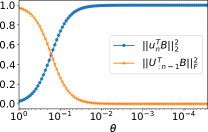
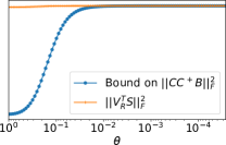
Figure 1: Behavior of our method in an example of Altschuler et al. (2016), as $\theta$ varies in [1,0). Left: the norm of $B$ when projected onto the space spanned by the last left singular vector and the rest. Right: Lower bound of Theorem 5.1.

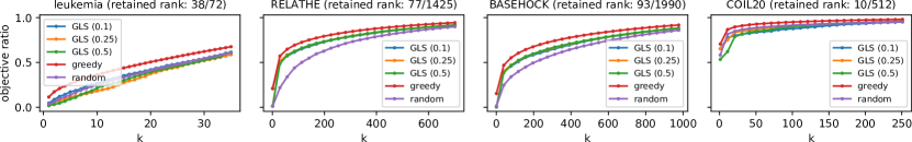
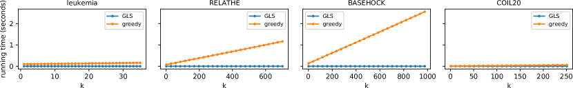
Figure 2: Performance analysis. Retained rank: no. of singular values accounting for 75% of $\|A\|_{F}^{2}$. Objective ratio: $\frac{\|CC^{+}B\|_{F}^{2}}{\|AA^{+}B\|_{F}^{2}}$.

We conduct experiments to gain further insight about our results. Throughout this section, we focus on GCSS and Algorithm 1, which we will call GLS.

A widely used algorithm in GCSS literature is the Greedy algorithm, which iteratively selects the best column from $A$ to add to $C$, such that $\|CC^{+}B\|_{F}^{2}$ is maximized. In practice, the Greedy algorithm can be implemented very efficiently and often provides good results (Farahat et al., 2011). While we have observed superior results from Greedy in terms of objective, our approach does offer certain advantages. We present experimental results to provide further insight on the behaviour of our algorithm, and to help determine when it may be an alternative to Greedy.

Can we outperform greedy? We consider an example by Altschuler et al. (2016), where the output of Greedy matches their quality guarantee.

Consider a set of orthogonal vectors $\{e_{0},e_{1},\dots,e_{n}\}$. We build a matrix $A$ with columns $e_{1},\theta e_{0}+e_{1}$, and $2\theta e_{0}+e_{j}$ for $j\geq 2$. The target matrix $B$ is comprised only of column $e_{0}$. Even though $B$ can be expressed using the first two columns of $A$, i.e., $e_{1},\theta e_{0}+e_{1}$, Greedy will pick $2\theta e_{0}+e_{t+1}$ at iteration $t$. To achieve a $(1-\epsilon)$-approximation of the optimum for $k=2$, it will need more than $\frac{1}{2\theta^{2}\epsilon}$ columns.

Does our approach fare any better? We analyze its behavior for varying values of $\theta$, in an instantiation of the above example of size $11\times 11$. In order to find the optimal column subset, comprised of columns 1 and 2, our algorithm needs to pick a singular vector subset $R$ such that the generalized leverage scores are high for these two columns.

In Figure 1 we plot key values for $\theta\in(0,1]$. On the left, we show the norm of $B$ projected onto the last left singular vector $u_{n}$, as well as on the rest, $U_{:n-1}$. As $\theta$ shrinks, the former rapidly approaches $1=\|B\|_{F}^{2}$, which indicates that $u_{n}$ is a good choice of $R$ (step 1 of Algorithm 1). On the right we plot the sum of the generalized leverage scores for columns 1 and 2, $\|V_{R}^{T}S\|_{F}^{2}$, and the lower bound on $\|CC^{+}B\|_{F}^{2}$, where $C=AS$, of Theorem 5.1. The leverage scores associated to $u_{n}$ always add up to almost 1. When $B$ projects well onto the space of $u_{n}$, the lower bound indicates that these two columns are a good choice. When $\theta$ is small, our algorithm will identify them for most values of $\epsilon,\delta$.

Quality-efficiency trade-off. We evaluate the performance of Algorithm 1 on a collection of real datasets, obtained from a repository maintained by Arizona State University for feature-selection tasks. We split each dataset in two. The first half of the columns acts as matrix $A$ (see def. of GCSS), and the second as $B$.

We compare our method to Greedy and a uniformly-at-random baseline (averaged over 100 iterations).

We run a variation on Algorithm 1. To avoid large values of the ratio $\frac{\sigma_{\omega}}{\sigma_{\mu}}$, we only retain singular vectors paired with the leading singular values accounting for at least 75% of the total squared norm. As per Algorithm 1, one would then build the set $R$ based on the choice of $\delta$. which however can make it difficult to control the size of $R$, and thus the decay of leverage scores. We thus try setting the size of $R$ to a number of values: $1/10,1/4$ and $1/2$ of the retained rank. For each resulting $R$ we compute generalized leverage scores. We use the generalized-leverage-score ordering to build a column submatrix $C_{k}$ of size $k$, for a range of $k$ (depending on the dataset size). We measure both $\|C_{k}C_{k}^{+}V\|_{F}^{2}$ and the running time of both algorithms (Greedy and ours).

The results are shown in Figure 2. Greedy is clearly superior in terms of objective function. However, our approach is more efficient for large values of $k$, as it requires essentially constant computation time with respect to this parameter. On some datasets, the leverage scores are not informative and a random choice may perform better in expectation. This is consistent with our results, as in the absence of sharp decay, there are no guarantees for small column subsets (see Section 6). Our approach seems to perform better on high-dimensional, high-rank data.

8 Related Work

The concept of leverage scores can be traced back to statistical leverage, long employed in statistics and the analysis of linear regression (Chatterjee & Hadi, 1986). The statistical leverages of a matrix, defined as the diagonal entries of the projector onto its row space, determine the influence of each row on the solution of a least-squares problem; hence “leverage.” It is not difficult to see that the leverage scores of a matrix’s columns correspond to the statistical leverages of a related matrix; see Equation (14).

The idea of using leverage scores to find good column subsets has its origins in randomized algorithms for fast matrix multiplication and $\ell_{2}$ regression (Drineas et al., 2006a, b). These methods sample rows or columns of the input matrices with probability proportional to their norms, to then solve the given tasks on the subsampled matrices with accuracy guarantees. It was later observed that similar strategies could be employed to compute approximate matrix factorizations, such as CUR (Mahoney & Drineas, 2009). For this purpose, rows and columns are sampled with probabilities proportional to their leverage scores (Drineas et al., 2008). A similar approach yields approximation algorithms for column subset selection (Boutsidis et al., 2009). Leverage scores can also be used for the design of deterministic algorithms (Papailiopoulos et al., 2014). The results presented in our paper allows us to extend the approach of Papailiopoulos et al. (2014) to other problems, as we argue in Section 5.1. Superior algorithms were later proposed for column subset selection (Guruswami & Sinop, 2012; Boutsidis et al., 2014). In addition, the greedy algorithm has attracted attention of its own (Çivril & Magdon-Ismail, 2012; Bhaskara et al., 2016), given its simplicity, efficiency and practical effectiveness (Farahat et al., 2011).

Recently, leverage scores have found applications in other areas, such as kernel methods (Schölkopf et al., 2002). Despite their potential for effective machine-learning algorithm design (Cortes & Vapnik, 1995), kernels often require handling large matrices. For that reason, sampling methods and approximate factorizations are often studied in this context. Leverage-score sampling has proven effective for this purpose (El Alaoui & Mahoney, 2015; Musco & Musco, 2016; Calandriello et al., 2017; Li et al., 2019; Erdélyi et al., 2020; Liu et al., 2020b). For a comprehensive review of this and related methods, see the article of Liu et al. (2020a). For overviews on the use of leverage scores and on randomized algorithms for matrix-related tasks, see the articles of Mahoney (2011) and Martinsson & Tropp (2020).

9 Conclusions

We have shown how the proposed generalized leverage scores, along with our novel results, can be used to design approximation algorithms for well-known problems. Our experimental results reveal that the proposed methods have certain advantages over known methods. Given the fundamental nature of the concept of generalized leverage scores and the numerous uses of standard leverage scores in the literature, we believe our contributions are likely to be taken further by the community in subsequent work.

Acknowledgements. This research is supported by Academy of Finland projects 317085 and 325117, the ERC Advanced Grant REBOUND (834862), the EC H2020 RIA project SoBigData++ (871042), and the Wallenberg AI, Autonomous Systems and Software Program (WASP) funded by the Knut and Alice Wallenberg Foundation.

Appendix

Proofs missing from the main text

Proof of Theorem 5.1. Throughout this proof, $r(A)$ denotes the column space of a given matrix $A$.

We can write $\|U_{R}^{T}B\|_{F}^{2}=\sum_{i}\|U_{R}^{T}b_{i}\|_{2}^{2}\geq\sum_{i}(1-\delta_{i})\|b_{i}\|_{2}^{2}$, for choices of $\delta_{i}$ such that $\|U_{R}^{T}b_{i}\|_{2}^{2}\geq(1-\delta_{i})\|b_{i}\|_{2}^{2}$, for $i=1,\dots,t$. This implies that for every $i$ there is a unit vector $u\in r(U_{R})$ satisfying $(u^{T}b_{i})^{2}\geq(1-\delta_{i})\|b_{i}\|_{2}^{2}$.

On the other hand, Theorem 4.4 guarantees that $\|CC^{+}U_{R}\|_{F}^{2}\geq|R|-\epsilon^{2}/4$. This implies that for every unit vector $u\in r(U_{R})$ there is a unit vector $w\in r(C)$ such that $(w^{T}u)^{2}\geq 1-\epsilon^{2}/4$.

It can be shown (Ordozgoiti et al., 2021) that for each $u\in r(U_{R})$, $w\in r(C)$ and $b_{i}$, where $u,w$ are unit vectors:

$$w^{T}b_{i}\geq u^{T}wu^{T}b_{i}-\sqrt{\left(1-(u^{T}w)^{2}\right)\left(\|b_{i}\|_{2}^{2}-(u^{T}b_{i})^{2}\right)}.$$

We get $(u^{T}w)^{2}\geq 1-\epsilon^{2}/4$ and $(u^{T}b_{i})^{2}\geq(1-\delta_{i})\|b_{i}\|_{2}^{2}$.

Thus, for every $b_{i}$ we can choose $u,w$ so that

$$(w^{T}b_{i})^{2} \geq\left(\sqrt{(1-\epsilon^{2}/4)(1-\delta_{i})\|b_{i}\|_{2}^{2}}-\sqrt{\frac{\epsilon^{2}}{4}\delta_{i}\|b_{i}\|_{2}^{2}}\right)^{2}$$

$$=(1-\epsilon^{2}/4)(1-\delta_{i})\|b_{i}\|_{2}^{2}+\frac{\epsilon^{2}}{4}\delta_{i}\|b_{i}\|_{2}^{2}$$

$$\quad-2\sqrt{(1-\epsilon^{2}/4)(1-\delta_{i})\frac{\epsilon^{2}}{4}\delta_{i}}\|b_{i}\|_{2}^{2}$$

$$=(1-\epsilon^{2}/4)(1-\delta_{i})\|b_{i}\|_{2}^{2}$$

$$\quad-\sqrt{\frac{\epsilon^{2}}{4}\delta_{i}}\|b_{i}\|_{2}^{2}\left(2\sqrt{(1-\epsilon^{2}/4)(1-\delta_{i})}-1\right)$$

$$\geq(1-\epsilon^{2}/4)(1-\delta_{i})\|b_{i}\|_{2}^{2}-\sqrt{\frac{\epsilon^{2}}{4}\delta_{i}}\|b_{i}\|_{2}^{2}$$

$$\geq(1-\epsilon^{2}/4)(1-\delta_{i})\|b_{i}\|_{2}^{2}-\sqrt{\frac{\epsilon^{2}}{4}}\|b_{i}\|_{2}^{2}$$

$$=(1-\epsilon^{2}/4)(1-\delta_{i})\|b_{i}\|_{2}^{2}-\frac{\epsilon}{2}\|b_{i}\|_{2}^{2}$$

It follows from the previous exposition that for adequate choices of $w_{i}$ in the column space of $C$,

$$\|CC^{+}B\|_{F}^{2} =\sum_{i=1}^{t}(w_{i}^{T}b_{i})^{2}$$

$$\geq\sum_{i=1}^{t}(1-\epsilon^{2}/4)(1-\delta_{i})\|b_{i}\|_{2}^{2}-\frac{\epsilon}{2}\|b_{i}\|_{2}^{2}$$

$$=(1-\epsilon^{2}/4)(1-\delta)\|B\|_{F}^{2}-\frac{\epsilon}{2}\|B\|_{F}^{2}.$$

Finally,

$$(1- \epsilon^{2}/4)(1-\delta)\|B\|_{F}^{2}-\frac{\epsilon}{2}\|B\|_{F}^{2}$$

$$=(1-\delta)\|B\|_{F}^{2}-(1-\delta)\frac{\epsilon^{2}}{4}\|B\|_{F}^{2}-\frac{\epsilon}{2}\|B\|_{F}^{2}$$

$$\geq(1-\delta)\|B\|_{F}^{2}-\frac{\epsilon}{2}\left(\frac{\epsilon}{2}\|B\|_{F}^{2}+\|B\|_{F}^{2}\right)$$

$$=(1-\delta)\|B\|_{F}^{2}-\|B\|_{F}^{2}\frac{\epsilon}{2}\left(\frac{\epsilon}{2}+1\right)$$

$$\geq(1-\delta)\|B\|_{F}^{2}\left(1-\frac{\epsilon}{2}\left(\frac{\epsilon}{2}+1\right)\right)$$

$$\geq(1-\delta)\|B\|_{F}^{2}\left(1-2\frac{\epsilon}{2}\right).$$

$$=(1-\delta)\|B\|_{F}^{2}(1-\epsilon).$$

∎

Quality-efficiency tradeoff results for the rest of the datasets

In Figures 3 and 4 we plot the objective ratio and the running time for a larger number of datasets. Greedy remains the better option if measured by the objective function. Our algorithm, GLS, performs better on high rank data sets, in line with previous observations. In some cases uniform sampling performs better. This reinforces our previous observation that for some datasets, the leverage scores computed the chosen set $R$ are not informative. We note here that more careful tuning may have served to achieve better results, and thus leave a more thorough empirical evaluation for future work.

With respect to running time (figure 4), the results are in line with what we would expect. With respect to $k$, Greedy scales linearly with $k$ but GLS remains essentially constant.

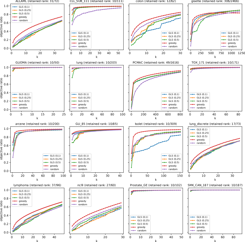
Figure 3: Objective ratio for values of $k$ on the rest of the datasets

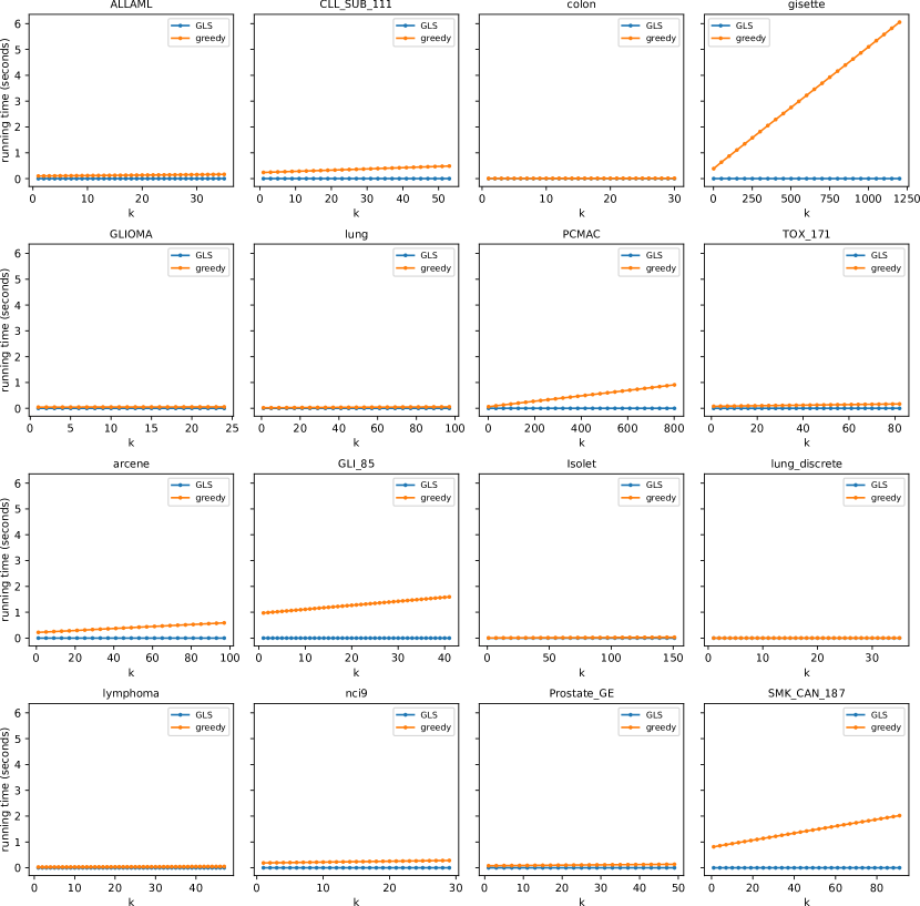
Figure 4: Running times for values of $k$ on the rest of the datasets

References

- Altschuler et al. (2016) Altschuler, J., Bhaskara, A., Fu, G., Mirrokni, V., Rostamizadeh, A., and Zadimoghaddam, M. Greedy column subset selection: New bounds and distributed algorithms. In International conference on machine learning, pp. 2539–2548. PMLR, 2016.
- Bhaskara et al. (2016) Bhaskara, A., Rostamizadeh, A., Altschuler, J., Zadimoghaddam, M., Fu, T., and Mirrokni, V. Greedy column subset selection: New bounds and distributed algorithms. 2016.
- Björck & Golub (1973) Björck, Å. and Golub, G. H. Numerical methods for computing angles between linear subspaces. Mathematics of computation, 27(123):579–594, 1973.
- Boutsidis et al. (2009) Boutsidis, C., Mahoney, M. W., and Drineas, P. An improved approximation algorithm for the column subset selection problem. In Proceedings of the Twentieth Annual ACM-SIAM Symposium on Discrete Algorithms, SODA ’09, pp. 968–977, USA, 2009. Society for Industrial and Applied Mathematics.
- Boutsidis et al. (2014) Boutsidis, C., Drineas, P., and Magdon-Ismail, M. Near-optimal column-based matrix reconstruction. SIAM Journal on Computing, 43(2):687–717, 2014.
- Calandriello et al. (2017) Calandriello, D., Lazaric, A., and Valko, M. Distributed adaptive sampling for kernel matrix approximation. In Artificial Intelligence and Statistics, pp. 1421–1429. PMLR, 2017.
- Chatterjee & Hadi (1986) Chatterjee, S. and Hadi, A. S. Influential observations, high leverage points, and outliers in linear regression. Statistical science, pp. 379–393, 1986.
- Civril (2014) Civril, A. Column subset selection problem is ug-hard. Journal of Computer and System Sciences, 80(4):849–859, 2014.
- Cortes & Vapnik (1995) Cortes, C. and Vapnik, V. Support-vector networks. Machine learning, 20(3):273–297, 1995.
- Deshpande et al. (2006) Deshpande, A., Rademacher, L., Vempala, S., and Wang, G. Matrix approximation and projective clustering via volume sampling. Theory of Computing, 2(1):225–247, 2006.
- Drineas et al. (2006a) Drineas, P., Kannan, R., and Mahoney, M. W. Fast monte carlo algorithms for matrices i: Approximating matrix multiplication. SIAM Journal on Computing, 36(1):132–157, 2006a.
- Drineas et al. (2006b) Drineas, P., Mahoney, M. W., and Muthukrishnan, S. Sampling algorithms for l 2 regression and applications. In Proceedings of the seventeenth annual ACM-SIAM symposium on Discrete algorithm, pp. 1127–1136, 2006b.
- Drineas et al. (2008) Drineas, P., Mahoney, M. W., and Muthukrishnan, S. Relative-error cur matrix decompositions. SIAM Journal on Matrix Analysis and Applications, 30(2):844–881, 2008.
- El Alaoui & Mahoney (2015) El Alaoui, A. and Mahoney, M. W. Fast randomized kernel ridge regression with statistical guarantees. In NIPS, 2015.
- Erdélyi et al. (2020) Erdélyi, T., Musco, C., and Musco, C. Fourier sparse leverage scores and approximate kernel learning. arXiv preprint arXiv:2006.07340, 2020.
- Farahat et al. (2011) Farahat, A. K., Ghodsi, A., and Kamel, M. S. An efficient greedy method for unsupervised feature selection. In 2011 IEEE 11th International Conference on Data Mining, pp. 161–170. IEEE, 2011.
- Golub & Van Loan (1996) Golub, G. H. and Van Loan, C. F. Matrix computations. edition, 1996.
- Guruswami & Sinop (2012) Guruswami, V. and Sinop, A. K. Optimal column-based low-rank matrix reconstruction. In Proceedings of the twenty-third annual ACM-SIAM symposium on Discrete Algorithms, pp. 1207–1214. SIAM, 2012.
- Hager (1989) Hager, W. W. Updating the inverse of a matrix. SIAM review, 31(2):221–239, 1989.
- Hardoon & Shawe-Taylor (2011) Hardoon, D. R. and Shawe-Taylor, J. Sparse canonical correlation analysis. Machine Learning, 83(3):331–353, 2011.
- Hotelling (1936) Hotelling, H. Relations between two sets of variates. Biometrika, 28(3/4):321–377, 1936. ISSN 00063444. URL http://www.jstor.org/stable/2333955.
- Li et al. (2019) Li, Z., Ton, J.-F., Oglic, D., and Sejdinovic, D. Towards a unified analysis of random fourier features. In International Conference on Machine Learning, pp. 3905–3914. PMLR, 2019.
- Liu et al. (2020a) Liu, F., Huang, X., Chen, Y., and Suykens, J. A. Random features for kernel approximation: A survey on algorithms, theory, and beyond. arXiv preprint arXiv:2004.11154, 2020a.
- Liu et al. (2020b) Liu, F., Huang, X., Chen, Y., Yang, J., and Suykens, J. Random fourier features via fast surrogate leverage weighted sampling. In Proceedings of the AAAI Conference on Artificial Intelligence, volume 34, pp. 4844–4851, 2020b.
- Mahoney (2011) Mahoney, M. W. Randomized algorithms for matrices and data. arXiv preprint arXiv:1104.5557, 2011.
- Mahoney & Drineas (2009) Mahoney, M. W. and Drineas, P. Cur matrix decompositions for improved data analysis. Proceedings of the National Academy of Sciences, 106(3):697–702, 2009.
- Martinsson & Tropp (2020) Martinsson, P.-G. and Tropp, J. A. Randomized numerical linear algebra: Foundations and algorithms. Acta Numerica, 29:403–572, 2020.
- Musco & Musco (2016) Musco, C. and Musco, C. Recursive sampling for the nystr” om method. arXiv preprint arXiv:1605.07583, 2016.
- Ordozgoiti et al. (2021) Ordozgoiti, B., Pai, S., and Kołczyńska, M. Insightful dimensionality reduction with very low rank variable subsets. In Proceedings of the Web Conference 2021, pp. 3066–3075, 2021.
- Papailiopoulos et al. (2014) Papailiopoulos, D., Kyrillidis, A., and Boutsidis, C. Provable deterministic leverage score sampling. In Proceedings of the 20th ACM SIGKDD international conference on Knowledge discovery and data mining, pp. 997–1006, 2014.
- Schölkopf et al. (2002) Schölkopf, B., Smola, A. J., Bach, F., et al. Learning with kernels: support vector machines, regularization, optimization, and beyond. MIT press, 2002.
- Shitov (2017) Shitov, Y. Column subset selection is np-complete. arXiv preprint arXiv:1701.02764, 2017.
- Uurtio et al. (2017) Uurtio, V., Monteiro, J. M., Kandola, J., Shawe-Taylor, J., Fernandez-Reyes, D., and Rousu, J. A tutorial on canonical correlation methods. ACM Computing Surveys (CSUR), 50(6):1–33, 2017.
- Çivril & Magdon-Ismail (2012) Çivril, A. and Magdon-Ismail, M. Column subset selection via sparse approximation of svd. Theoretical Computer Science, 421:1 – 14, 2012. ISSN 0304-3975. doi: https://doi.org/10.1016/j.tcs.2011.11.019. URL http://www.sciencedirect.com/science/article/pii/S0304397511009388.