Pseudospectrum and binary black hole merger transients

Abstract

The merger phase of binary black hole coalescences is a transient between an initial oscillating regime (inspiral) and a late exponentially damped phase (ringdown). In spite of the non-linear character of Einstein equations, the merger dynamics presents a surprisingly simple behaviour consistent with effective linearity. On the other hand, energy loss through the event horizon and by scattering to infinity renders the system non-conservative. Hence, the infinitesimal generator of the (effective) linear dynamics is a non-selfadjoint operator. Qualitative features of transients in linear dynamics driven by non-selfadjoint (in general, non-normal) operators are captured by the pseudospectrum of the time generator. We propose the pseudospectrum as a unifying framework to thread together the phases of binary black hole coalescences, from the inspiral-merger transition up to the late quasinormal mode ringdown.

1 Binary black hole simple dynamics: effective linearity

Non-linear general relativistic dynamics controlling the binary black hole (BBH) merger leads to a remarkably simple waveform. This fact raises the question about the possibility of describing the dominating features of BBH waveforms in terms of appropriate effective linear dynamics. Such a perspective has been recently advocated in [46, 47] to address the simplicity and universality of BBH dynamics. Here we explore such an effective linearity assumption, when further complemented with the non-conservative character of the underlying BBH dynamics. Specifically, we propose the non-modal analysis approach to dynamical transients [80, 74], built on the notion of pseudospectrum and non-normal linear dynamics [81], as a systematic and unifying framework for the different regimes of BBH waveforms.

The potential role of effective linearity in BBH dynamics is by no means a new idea . Early educated expectations based on the non-linearity of the theory suggested complicated patterns in the BBH merger waveform (cf. e.g. [75], namely the iconic Thorne’s Fig. 1). This situation changed drastically in 2005 with the numerical BBH breakthroughs [70], ultimately confirmed a decade later by observations [1], that revealed a simple BBH waveform. However, aspects of such a simplicity were already present in the previous literature, as illustrated by the intuitions coming from the analysis of the GW emission from point-particle falling into a BH [25] or the Damour’s “effacement property” [22] hiding the details in the binary dynamics. In particular, the latter stands in a line of thinking culminating in the Effective-One-Body framework [16, 15], that provides an effective description of the BBH waveform that maps the full dynamics to ordinary differential equations structures and whose extraordinary success provides one of the strongest indications of the underlying simplicity. Of particular interest in our present setting is the “close-limit” approximation introduced by Pullin and Price [72, 33, 52], in which the merger BBH spacetime is shown to be extremely well captured by the perturbation of a single black hole, therefore providing an explicit realisation of ‘effective linearity’ in BBH mergers . Most importantly, recent additional support to an effective linear regime valid not only at late ringdown BBH waveforms but starting as early as the merger  is advocated by comparing with accurate full BBH simulations in [32] and, crucially, with observations [43, 18]. The latter results are not exempt of controversy (specially, regarding the detectability of quasinormal mode (QNM) overtones [18, 30, 20, 41, 73, 29]), but the idea that some kind of effective linearity plays a role in BBH dynamics has indeed entered in current research [60]. In brief, BBH waveforms seem more ‘linear’ than expected, raising the question if the transient phenomenon describing the passage from the inspiral to the late ringdown, through the merger phase, can be described in terms of effective linear dynamics.

The last statement is a bold one. Indeed, transients are typically associated with non-linear and/or time-dependent dynamics. Along this line, recent insightful studies on ringdown dynamics [73] stress precisely the importance of non-linearities to account for full BH QNM dynamics. However, this is not in contradiction with the possibility that some of the (dominating) qualitative mechanisms may be driven by effectively linear dynamics. Even more, one can argue  that if a sufficiently good control of appropriate underlying background BBH dynamics is available, then BBH waveform features may be indeed well described in terms of linear dynamics over that dynamical background. The key point is then the correct identification of the relevant background dynamics. A particular approach to this problem, based on notions of integrability theory, is proposed in Ref. [47]. Here, we rather adopt an agnostic position regarding the choice of dynamical background, aiming at introducing a framework to assess to capability of effective linear dynamics to account for BBH transients.

Specifically we build on the known fact [81] that, in parallel and complementarily to non-linear dynamics, purely linear mechanisms can indeed be responsible of transient growth behaviour even if the spectrum of the linearized (time-frozen) operator generating time dynamics stays in the stable regime of the complex plane. The reason can be traced to a non-intuitive, but basic fact, in linear algebra: linear combinations of exponentially damped eigenvectors can present an initial transitory growth before fully decaying, as long as they are non-orthogonal (cf. e.g. [74]). In other words, if eigenfunctions  of the time generator are not orthogonal, purely linear transients can occur. Such non-orthogonality of eigenfunctions characterizes the operator as non-normal. In contrast with the normal case, in particular for unitary operators in conservative dynamics, the decay properties are not fully captured by the spectrum, so a modal (eigenvalue) analysis is not appropriate along the full time evolution. The late time dynamics is still controlled by the spectrum, but initial and intermediate time regimes require information of the full operator in a non-modal analysis approach, intimately related to the notion of pseudospectrum [81, 24, 76]. Such a perspective has proved very illuminating in the study of hydrodynamic instability theory and the onset of turbulence in fluid dynamics [80, 74, 81], thus proving that strong transient growths are not necessarily due to non-linearities but can be accounted for by linear dynamics if the latter are non-normal.

Here we explore the applicability of such non-modal approach to BBH merger dynamics. Indeed, due to asymptotic radiative losses and flows through the horizon, the effective ‘near-zone’ BBH dynamics are non-conservative. This loss of unitarity entails the non-selfadjoint character of the infinitesimal time generator that, in generic situations, will be a non-normal operator. Under the assumption of effective linear BBH dynamics we are therefore in the natural setting to apply non-modal analysis to the study of transient growth in BBH mergers.

2 Transients and pseudospectrum

2.1 Non-normal linear dynamics and transient growth

Let us consider the following linear dynamical system

$$\left\{\begin{array}[]{l}\partial_{t}u=Au\\ u(t=0)=u_{0}\end{array}\right.$$ (3)

with $A$ an operator acting on functions $u$ in an appropriate Hilbert space $H$, with scalar product $\langle\cdot,\cdot\rangle$ and norm $||\cdot||$. We write formally the solution to the evolution problem as

$$u(t)=e^{tA}u_{0}\ .$$ (4)

We are interested in monitoring the maximum growth rate of solutions $u(t)$ in time, namely

$$G(t)=\sup_{u_{0}\neq 0}\frac{||u(t)||}{||u_{0}||}=\sup_{u_{0}\neq 0}\frac{||e^{tA}u_{0}||}{||u_{0}||}=||e^{tA}||\ ,$$ (5)

where in the last equation we make use of the operator norm induced from the vector norm $||\cdot||$. The late time behaviour of $G(t)$ is always described by the spectrum $\sigma(A)$ of $A$. To fix ideas and assuming $\sigma(A)$ composed only by eigenvalues , at late times $G(t)$ is controlled by the slowest decaying eigenvalue $\lambda_{0}$ of $A$, namely that one with largest real part, so $||e^{tA}||\sim e^{t\mathrm{Re}(\lambda_{0})}$. Late time stability occurs for $\mathrm{Re}(\lambda_{0})<0$. However, if we are interested in $G(t)$ along the whole evolution, the spectrum $\sigma(A)$ is not enough. Assuming diagonalisability and writing $A=P\Lambda P^{-1}$, with $\Lambda$ diagonal given by the eigenvalues of $A$ and $P$ constructed from the corresponding eigenfunctions, we can write

$$G(t)=||e^{tA}||=||Pe^{t\Lambda}P^{-1}||\ .$$ (6)

If $P$ is unitary, i.e. if the eigenfunctions are orthonormal, then indeed $||P||=1$ (in the norm associated with $\langle\cdot,\cdot\rangle$) and $G(t)$ is well estimated by the spectrum $\sigma(A)$, namely $G(t)\sim||e^{t\Lambda}||$ and we can do standard spectral (modal) analysis. In particular, the evolution of linear combinations of orthogonal eigenfunctions associated with eigenvalues with negative real part is monotonically decreasing. On the contrary, if eigenfunctions of $A$ are non-orthogonal (i.e. if $A$ is non-unitarily diagonalisable and therefore non-normal), the spectrum $\sigma(A)$ is not enough to control $G(t)$ and the full operator $e^{tA}$, in particular eigenfunctions of $A$ in $P$ —cf. Eq. (6)— must be considered. Crucially, the evolution of linear combinations of non-orthogonal eigenfunctions can lead to transient growths, in a purely linear mechanism, even if associated eigenvalues have negative real part: a genuine non-modal analysis phenomenon.

2.2 Non-modal analysis: spectrum, numerical range and pseudospectrum

Three sets in the complex plane $\mathbb{C}$, associated with $A$, play a relevant role in the discussion: the spectrum $\sigma(A)$, the numerical range $W(A)$ and, fundamentally, the $\epsilon$-pseudospectra $\sigma^{\epsilon}(A)$. Of special relevance are the suprema of the real parts of each respective set. Specifically:

• Spectrum $\sigma(A)$. Namely the set of $\lambda\in\mathbb{C}$ where the resolvent $R_{A}(\lambda)=(A-\lambda I)^{-1}$ is not defined as a bounded operator. The spectral abscissa $\alpha(A)$ is defined by

  $$\alpha(A) = \sup\mathrm{Re}\big{(}\sigma(A)\big{)}=\sup\{\mathrm{Re}(\lambda),\hbox{with}\ \lambda\in\sigma(A)\}\ .$$ (7)

  In the QNM context $\alpha(A)$ corresponds to the so-called spectral gap.

• Numerical range $W(A)$. This set depends on the scalar product and is defined as

  $$W(A)=\{\langle u,Au\rangle,\hbox{with}\ ||u||=1,u\in H\}\ .$$ (8)

  The numerical abscissa $\omega(A)$ is defined as

  $$\omega(A) = \sup\mathrm{Re}\big{(}W(A)\big{)}=\sup\{\mathrm{Re}(\lambda),\hbox{with}\ \lambda\in W(A)\}\ .$$ (9)

  A very useful characterization, cf. e.g. [81], is (here $A^{\dagger}$ is the adjoint of $A$ through $\langle\cdot,\cdot\rangle$)

  $$\omega(A)=\sup\sigma\left(\frac{1}{2}(A+A^{\dagger})\right)\ .$$ (10)

• $\epsilon$-Pseudospectrum $\sigma^{\epsilon}(A)$. This is the fundamental notion in the present setting. As $W(A)$ and in contrast with the spectrum, it depends on the choice of scalar product [31]. It admits different characterizations, each one stressing a complementary aspect

  $$\sigma^{\epsilon}(A) = \{\lambda\in\mathbb{C}:||R_{A}(\lambda)||=||\lambda\mathrm{Id}-A)^{-1}||>1/\epsilon\}$$

  $$= \{\lambda\in\mathbb{C},\exists v\in H:||Av-\lambda v||<\epsilon,||v||=1\}$$

  $$= \{\lambda\in\mathbb{C},\exists\;\delta A\ \hbox{bounded operator},||\delta A||<\epsilon:\lambda\!\in\!\sigma(A+\delta A)\}$$

  The first one characterizes $\epsilon$-pseudospectra as sets bounded by the contour levels of the norm of the resolvent $R_{A}(\lambda)$ (as a function in the $\lambda$-complex plane), the second introduces the notion of $\epsilon$-quasimode $v$, whereas the latter permits to address the spectral instability under perturbations $\delta A$ of $A$. The key feature in the present setting is that, even if the spectrum $\sigma(A)$ lays in the stable left-half of $\mathbb{C}$, growth transients can happen if the $\epsilon$-pseudospectra $\sigma^{\epsilon}(A)$ sets protrude significantly in the unstable right-half plane. This leads to the introduction, for each $\epsilon>0$, of the pseudospectral abscissa

  $$\alpha_{\epsilon}(A) = \sup\mathrm{Re}\big{(}\sigma^{\epsilon}(A)\big{)}=\sup\{\mathrm{Re}(\lambda),\hbox{with}\ \lambda\in\sigma^{\epsilon}(A)\}\ .$$ (12)

The relevance of these three sets is that they control, at different time regimes, the maximum growth rate $G(t)=||e^{tA}||$ of solutions $u(t)$ to Eq. (3). Specifically, the spectrum $\sigma(A)$ controls the late $t\to\infty$ limit through the spectral abscissa $\alpha(A)$, whereas the numerical range $W(A)$ controls the initial growth as $t\to 0^{+}$, through the numerical abscissa $\omega(A)$. The key structural role of the $\epsilon$-pseudospectrum notion arises from the fact that it interpolates between late times controlled by $\sigma(A)$ (in the $\epsilon\to 0$ limit) and early times controlled by $W(A)$ (in the $\epsilon\to\infty$ limit), providing a control of the growth rate at intermediate times in terms of the pseudospectral abscissa $\alpha_{\epsilon}(A)$, for the whole range $\epsilon\in\;]0,\infty[$. In this sense, since it takes into account the full structure of $A$ and not only its spectrum, the $\epsilon$-pseudospectrum is the relevant object to consider in generic non-normal dynamics, recovering the standard spectral approach for normal (e.g. unitary) dynamics by taking $\epsilon\to 0$, since $\sigma(A)=\lim_{\epsilon\to 0}\sigma_{\epsilon}(A)$.

2.3 The transient dynamical regimes and the pseudospectrum

We make explicit now the relation of $\sigma(A)$, $W(A)$ and $\sigma_{\epsilon}(A)$ with respective time regimes:

• Triggering of the transient: numerical abscissa $\omega(A)$.

  The initial slope in the maximal growth factor $G(t)=||e^{tA}||$ is given by [81]

  $$\frac{d}{dt}\left.||e^{tA}||\right|_{t=0}=\lim_{t\to 0^{+}}\frac{1}{t}\ln||e^{tA}||=\omega(A)\ .$$ (13)

  As indicated above, this initial growth is controlled by $\epsilon$-pseudospectra in the $\epsilon\to\infty$ limit, specifically by the depart of the pseudospectral abscissa from an $\epsilon$-linear behaviour

  $$\omega(A)=\lim_{\epsilon\to\infty}\left(\alpha_{\epsilon}(A)-\epsilon\right)\ .$$ (14)

  This confers the numerical abscissa $\omega(A)$ with the significant role of detecting the possibility of the triggering of a growth transient. Moreover, using the characterization of $\omega(A)$ in (10), in the case that $\omega(A)$ is realised as a maximum and not only the supremum, the corresponding eigenvector $u_{\omega(A)}$ of the maximum eigenvalue — i.e. $\omega(A)$ — in

  $$\left(\frac{1}{2}(A+A^{\dagger}\right)u_{\omega(A)}=\omega(A)u_{\omega(A)}\ ,$$ (15)

  realizes the maximum possible growth in $||e^{tA}||$ at $t=0$. Thus, the choice of initial data

  $$u_{0}:=u_{\omega(A)}\ ,$$ (16)

  in Eq. (3) provides the candidate for the initial data with strongest initial growth transient.

  Finally, the numerical abscissa provides an upper bound for the growth factor [81]

  $$||e^{tA}||\leq e^{t\omega(A)}\ ,\ \forall t\geq 0\ ,$$ (17)

  holding along the transient. In particular, $\omega(A)=0$ characterises $A$ as contractive

  $$||e^{tA}||\leq 1\ ,\ \forall t\geq 0\quad\hbox{if and only if}\quad\omega(A)=0\ .$$ (18)

• Transient peak estimations: pseudospectral abscissa $\alpha_{\epsilon}(A)$ and Kreiss constant ${\cal K}(A)$

  The pseudospectrum provides a tool for a qualitative understanding of the transient process at intermediate times. In particular, a lower bound for the peak in the transient growth is given in terms of the pseudospectral abscissa $\alpha_{\epsilon}(A)$ for any $\epsilon>0$, namely

  $$\sup_{t\geq 0}||e^{tA}||\geq\frac{\alpha_{\epsilon}(A)}{\epsilon}\quad,\quad\forall\epsilon>0\ .$$ (19)

  This means that large values of the resolvent in the right half-complex plane, with dependences in $\epsilon$ of the $\epsilon$-pseudospectrum $\sigma_{\epsilon}(A)$ stronger than linear (normal operator), lead to transient growths even if the spectrum $\sigma(A)$ is well inside the stable left half-plane. In practice [74, 81], if the resolvent norm is found to be $||R_{A}(z)||=||(z-A)^{-1}||=:S$ for a $z\in\mathbb{C}$ with $\mathrm{Re}(z)=1/\Delta T$ then, taking $\epsilon:=1/S$ and using the first characterization of the $\epsilon$-pseudospectrum in (iii)), it holds $\mathrm{Re}(z)\leq\alpha_{\epsilon}(A)$ and, from (19)

  $$\sup_{t\geq 0}||e^{tA}||\geq\frac{\alpha_{\epsilon}(A)}{\epsilon}\geq\frac{\mathrm{Re}(z)}{\epsilon}=\frac{1}{\epsilon\;\Delta T}=\frac{S}{\Delta T}\ .$$ (20)

  The quantity $\Delta T$ admits a dynamical interpretation, akin to that in modal analysis [81]: transients with growth bounded below by (20) will actually happen in a time scale $\Delta T$.

  A tighter lower bound for the transient growth can be obtained by maximizing over $\epsilon>0$, leading to a lower bound in terms of the so-called Kreiss constant ${\cal K}(A)$, namely

  $$\sup_{t\geq 0}||e^{tA}||\geq{\cal K}(A)\ ,$$ (21)

  where ${\cal K}(A)$ is defined — and usefully characterised in terms of the resolvant norm— as

  $${\cal K}(A):=\sup_{\epsilon>0}\left\{\frac{\alpha_{\epsilon}(A)}{\epsilon}\right\}=\sup_{\mathrm{Re}(z)>0}\{|\mathrm{Re}(z)|\cdot||(z-A)^{-1}||\}\ .$$ (22)

  Finer dynamical bounds in bounded time intervals $0<t\leq\tau$ can be found in [81, 23]. Finally, notice that in the case $\omega(A)=0$, we have that inequality (21) is sharp, with $\sup_{t\geq 0}||e^{tA}||={\cal K}(A)=1$. This unity bound is attained at $t=0$ for $\sup_{t\geq 0}||e^{tA}||$, as follows from inequality (18), and in the limit $\epsilon\to\infty$ for ${\cal K}(A)=1$, as seen in (14).

• Late time behaviour: spectral abscissa or spectral gap $\alpha(A)$.

  The spectrum $\sigma(A)$ controls the late transient behaviour in both normal and non-normal dynamics. Specifically, the late time asymptotics are controlled by the spectral abscissa

  $$\lim_{t\to\infty}\frac{1}{t}\ln||e^{tA}||=\alpha(A)=\lim_{\epsilon\to 0}\alpha_{\epsilon}(A)\ ,$$ (23)

  The characterization in terms of the pseudospectral abscissa $\alpha_{\epsilon}(A)$ completes the interpolation role of the $\epsilon$-pseudospectrum from early ($\epsilon\to\infty$) to late time dynamics ($\epsilon\to 0$). For completitude, we note that a lower-bound counterpart of (17) is given by

  $$||e^{tA}||\geq e^{t\alpha(A)}\ ,\ \forall t\geq 0\ .$$ (24)

3 Pseudospectrum in the ‘close limit’ approximation to BBH mergers

Once we have discussed the role of $\epsilon$-pseudospectra in generic transients in non-normal linear dynamics, we explore the application of this framework to the BBH merger transient under the hypothesis of effective (non-normal) linear dynamics. Distinct physical mechanisms are in action along the different phases of the BBH dynamics—namely the initial inspiral, the merger phase itself and the late ringdown (cf. [75]). In this setting, the notion of $\epsilon$-pseudospectrum may offer a unifying perspective of the BBH dynamics and waveform through its different regimes, interpolating from the late inspiral corresponding to $\epsilon\to\infty$ to the late ringdown at $\epsilon\to 0$, passing through from the transitional merger at intermediate values of $\epsilon$. We note the inverse relation between the time scale $t_{\mathrm{dyn}}$ at each dynamical phase and $\epsilon$, namely

$$t_{\mathrm{dyn}}\sim\frac{1}{\epsilon}\ ,$$ (25)

that offers a qualitative tool to associate with particular structures/patterns in the pseudospectrum “topographic map” of the resolvent norm (cf. e.g. [50] for such a qualitative account of the pseudospectrum), with distinct dynamical phases in the BBH transient process.

Specifically, some features of the BBH dynamics where one may explore the capability of the $\epsilon$-pseudospectrum to offer qualitative/quantitative insights, include the following points:

• Characterization of the transition from the late inspiral to the merger.

• Estimation of the dominating peak at the merger.

• Identification of time scales for the transition from merger phase to the ringdown phase.

• Assessment of the possibility to account early/late dynamical behaviours in the merger transient process in terms of the specifics of the resulting final merged BH.

Exploring these points requires adopting a particular setting in which the pseudospectrum can be concretely realised. Very different scenarios, with distinct degrees of complexity, can be envisaged (cf. e.g. [46, 47]). In the following, as a first exploratory stage, we adopt an approach in the spirit of the “close-limit” approximation [72, 33, 52] to BBH mergers.

3.1 BBH merger transient in the “close-limit” approach

As referred in the introduction, the “close-limit” approximation [72, 33, 52] provides a model for the BBH coalescence dynamics, starting from the merger phase, in terms of the linear perturbations of the resulting merged and eventually stationary BH. In the long path leading to the successful numerical BBH mergers [70, 71], this model contributed by offering key insights into the emitted waveforms and estimations of released energy. Interestingly, once the BBH problem is under numerical control and actual observational data are available, revisiting such models can be key to understand the physical mechanisms underlying the BBH problem.

Our treatment here dwells in a “close limit” spirit, realised in the hyperboloidal setting to BH perturbations pioneered by A. Zengınoglu [83, 84] and M. Ansorg and R.P. Macedo [65, 2], specifically in the form championed by R.P. Macedo [66, 63, 64, 50]. For simplicity, in this first exploratory attempt we stay in a spherically symmetric Schwarzschild setting. Following the discussion and the notation in reference [50], the relevant evolution equation is

$$\left\{\begin{array}[]{l}\partial_{\tau}u=iLu\\ u(\tau=0,x)=u_{0}(x)\end{array}\right.\quad,\quad\hbox{with}\quad u(\tau,x)=\begin{pmatrix}\phi(\tau,x)\\ \psi(\tau,x)\end{pmatrix}$$ (28)

where the $\tau$ time parameter is adapted to hyperboloidal slices and Eq. (28) is the first-order reduction in time of the linear wave equation for $\phi$, with $\psi=\partial_{\tau}\phi$, where $\phi$ is an $(\ell,m)$ spherical harmonic mode of the axial/polar scalar master functions. The operator $L$ writes as

$$L=\frac{1}{i}\!\left(\begin{array}[]{c|c}0&1\\ \hline\cr L_{1}&L_{2}\end{array}\right)\ ,$$ (31)

where the explicit form of operators $L_{1}$ and $L_{2}$ is given by

$$L_{1}=\frac{1}{w(x)}\big{(}\partial_{x}\left(p(x)\partial_{x}\right)-\tilde{V}(x)\big{)}\;,\;L_{2}=\frac{1}{w(x)}\big{(}2\gamma(x)\partial_{x}+\partial_{x}\gamma(x)\big{)}\ ,$$ (32)

where $x\in[a,b]$ is a compactified radial coordinate along the hyperboloidal slice $\Sigma_{\tau}$, with $a$ and $b$ corresponding to the BH horizon and future null infinity ${I}^{+}$, the functions $p(x)$, $w(x)$ and $\gamma(x)$ are fixed by the choice of slicing and compactification along the hyperboloid, and $\tilde{V}(x)=V(x)/p(x)$, with $V(x)$ the effective potential corresponding to each gravitational parity (see [50] for details). Choosing an ‘energy scalar product’ (cf. [50, 31]) we can write

$$\langle u_{1},u_{2}\rangle_{{}_{E}}=\frac{1}{2}\int_{a}^{b}(w(x)\bar{\psi}_{1}\psi_{2}+p(x)\partial_{x}\bar{\phi}_{1}\partial_{x}\phi_{2}+\tilde{V}(x)\bar{\phi}_{1}\phi_{2})dx\ ,$$ (33)

that leads to the following expression for the formal adjoint $L^{\dagger}$ of $L$

$$L^{\dagger}=\frac{1}{i}\!\left(\begin{array}[]{c|c}0&1\\ \hline\cr L_{1}&L_{2}+L_{2}^{\partial}\end{array}\right)\!\ ,$$ (36)

with $L_{2}^{\partial}$ formally expressed in terms of Dirac-delta’s supported at the boundaries

$$L_{2}^{\partial}=2\frac{\gamma}{w}\bigg{(}\delta(x-a)-\delta(x-b)\bigg{)}\ .$$ (37)

In the following, we apply the elements discussed in section 2.3 to the transient case of BBH dynamics modelled in a (first-order) ‘close limit’ approximation captured by Eqs. (28)-(42).

3.2 BBH inspiral-merger transition

We start by exploring the possibility of describing the transition from the late inspiral phase to the merger phase by looking at the limit $\epsilon\to\infty$ of the pseudospectrum. A necessary condition for making sense of such a description is having an initial positive slope of the growth factor $||e^{i\tau L}||$, i.e. the positivity of its time derivative at $\tau=0$, that according to the characterisation in Eq. (13) translates into the positivity of the numerical abscissa. The latter is indeed characterised by the pseudospectrum in the $\epsilon\to\infty$ limit, as captured in Eq. (14).

First, in order to match the notation in section 2 — compare in particular the evolution equations (3) and (28) — we identify $A=iL$ that, at the spectral level, amounts to a $\pi/2$ rotation in the complex plane. In particular we can write (note $A^{\dagger}=-iL^{\dagger}$)

$$A=\left(\begin{array}[]{c|c}0&1\\ \hline\cr L_{1}&L_{2}\end{array}\right)\quad,\quad A^{\dagger}=-\left(\begin{array}[]{c|c}0&1\\ \hline\cr L_{1}&L_{2}+L_{2}^{\partial}\end{array}\right)\ .$$ (42)

Using these expressions for $A$ and $A^{\dagger}$ we can calculate the symmetric part of the $A$ operator

$$\!\!\!\!\!\!\!\!\!\!\!\!\!\!\!\!\!\!\frac{1}{2}(A+A^{\dagger})=\frac{1}{2}\left(\begin{array}[]{c|c}0&0\\ \hline\cr 0&-L_{2}^{\partial}\end{array}\right)=\left(\begin{array}[]{c|c}0&0\\ \hline\cr 0&-\displaystyle\frac{\gamma}{w}\bigg{(}\delta(x-a)-\delta(x-b)\bigg{)}\end{array}\right)\ ,$$ (47)

where we have used the expression of $L_{2}^{\partial}$ in Eq. (37). This remarkably simple expression corresponds to a diagonal operator (in particular, we can consider the representation of the Dirac-delta in terms of limits of appropriate functions). Therefore eigenvalues are given by the diagonal entries. In addition, and as a key consequence of the outgoing nature of the asymptotic boundary conditions —realised in the hyperboloidal slicing that reaches future null infinity ${I}^{+}$ and in the (outgoing) transverse character of the slicing at the BH horizon— it holds

$$-\frac{\gamma(a)}{w(a)}<0\quad,\quad\frac{\gamma(b)}{w(b)}<0\ .$$ (48)

From expressions (47) and (48), and using the spectral characterisation (10) of the numerical abscissa, in terms of the supremum of the real part of the spectrum of $\frac{1}{2}\left(A+A^{\dagger}\right)$, it follows

$$\omega(L)=0\ .$$ (49)

We notice that this result is essentially independent of the chosen foliation, only depending on asymptotic boundary values, actually the part responsible of the loss of selfadjointness of the operator as a consequence of the field leaking through the boundaries [50, 31]. Crucially, we notice that this result does not depend on the specific nature of the potential $V(x)$.

The blunt consequence of Eq. (49) is that no peak can happen in the later dynamical evolution. Therefore this simple model —namely, a first-order perturbation ‘close-limit’ BBH model— cannot account for the transition from the late inspiral to the merger phase. On the other hand, the fact that $\omega(L)$ is not negative, but strictly vanishing, entails a non-trivial consequence: $\omega(L)=0$ is consistent with a description in terms of non-normal linear dynamics starting at the merger peak. This is akin with the results in [32, 43, 18] and opens the possibility of exploring the full BBH dynamics from a non-modal analysis/pseudospectrum perspective right from the merger peak, as in the original close-limit approximation spirit.

3.3 Kreiss-constant characterisation of the BBH merger waveform maximum

Applying the discussion of the Kreiss constant ${\cal K}(L)$ in section 2.3 to BBH mergers, one would like to assess the possibility of estimating the merger peak from ${\cal K}(L)$. Unfortunately, this expectation does not stand in the close-limit approximation to BBH mergers. From the vanishing of the numerical abscissa in Eq. (49), we can conclude from (18) that $e^{itL}$ is contractive and, as discussed after Eq. (22), it holds ${\cal K}(L)=1$. We conclude that finer models than the first-order close-limit approximation are needed to explore the use of the Kreiss constant to estimate the merger peak in a non-normal linear description of BBH mergers.

With these more general BBH settings in mind, let us make some general considerations on the Kreiss constant and, more generically, on the $\epsilon$-pseudospectrum with intermediate $\epsilon$’s:

• Kreiss constant and pseudospectrum. For the sake of clarity, we translate the expression of ${\cal K}(A)$ in terms of $L$, namely performing a clockwise $\pi/2$-rotation in Eq. (22) we get

  $${\cal K}(L)=\sup_{\mathrm{Im}(z)<0}\{|\mathrm{Im}(z)|\cdot||(L-zI)^{-1}||\}\ .$$ (50)

  We notice that the evaluation of the Kreiss constant is straightforward (and comes “for free”) during the process of calculating the pseudospectrum numerically, since the latter consists precisely in evaluating the resolvent’s norm $||(L-zI)^{-1}||$ at each point $z\in\mathbb{C}$.

• Kreiss constant and gravitational wave strain at the merger peak. The Kreiss constant provides a lower bound estimate of the growth factor $G(t)$ in Eq. (5), namely the ratio between the amplitude of the propagating field $\phi(t)$ and an initial reference value. This dimensionless quantity should provide an estimation of the gravitational wave strain $h$

  $$h\gtrsim{\cal K}\ ,$$ (51)

• Pseudospectral abscissa timescale. The patterns appearing in the pseudospectrum inform about phenomena happening at different time scales. The discussion around expressions (20) can be recast in the BBH setting by introducing a $\epsilon$-pseudospectrum timescale as

  $$t_{\mathrm{\epsilon}}:=\frac{1}{\alpha_{\epsilon}(L)}$$ (52)

  where now $\alpha_{\epsilon}(L)=\sup|\mathrm{Im}(\sigma^{\epsilon}(L)|$. In other words, dynamical phenomena associated with a given $\epsilon$-pseudospectrum pattern manifests at a time scale $t_{\mathrm{\epsilon}}$. The inequality

  $$t_{\mathrm{\epsilon}}\cdot\epsilon\geq\left({\cal K}(L)\right)^{-1}\ ,$$ (53)

  following from (22) gives a more precise content  to the timescale estimate in (25).

3.4 Spectral abscissa: the question of QNM spectral (in)stability

The late time decay is controlled by the spectrum $\sigma(L)$ of $L$, namely the $\epsilon$-pseudospectrum $\sigma^{\epsilon}(L)$ in the limit $\epsilon\to 0$. This holds both for normal and non-normal dynamics. Specifically, at sufficiently late times the spectral abscissa $\alpha(L)$ controls the decay. In the asymptotically flat BH case the very late decay is driven by tails corresponding to the continuous part of the spectrum. Before the tails take over, the late decay is controlled by the imaginary part of the fundamental QNM. As discussed above, for earlier times the spectrum does not capture the dynamics in the non-normal case and intermediate $\epsilon$-pseudospectra are needed. A natural question concerns the role of QNM overtones in the BBH transient and ringdown dynamics.

The latter question, crucial in BH spectroscopy [8, 27, 5, 61, 43, 32, 42, 17, 54, 62], becomes particularly relevant in the context of the recent discussion of a possible instability of the QNM spectrum [50, 51, 31]. The BH pseudospectrum (in the ‘energy norm’) shows non-trivial patterns extending far from the spectrum. This is a signature of spectral instability. The analysis in refs. [50, 51, 31] suggests the presence of a QNM overtone instability under high-wave number (small scale) perturbations that, crucially, leaves the fundamental QNM (and therefore the QNM spectral abscissa’ $\alpha(L)$) unchanged. Another kind of (’flea on the elephant’) instability affecting the fundamental QNM has been proposed in [19] . However, these QNM instability proposals must address the fact that the global qualitative aspects of the time evolution after the BBH merger seems quite insensitive to such spectral instabilities.

3.5 Spectral and time-domain perspectives: QNMs and dynamics.

We discuss now some points aiming at reconciling these seemingly conflicting spectral and dynamical perspectives and, more generally, at shedding light on QNMs and dynamics:

• Pseudospectrum universality and early-intermediate time evolution. Before the late ringdown, the average qualitative aspects of the transient dynamics are not imprinted by possible perturbations of the QNM spectrum, in particular by perturbed QNM overtones. This fact is not surprising since, as discussed above, dynamics at early and intermediate timescales are not controlled by the spectrum ($\epsilon=0$) but by $\epsilon$-pseudospectra with large/intermediate $\epsilon$ values. In this setting, the following fact is crucial:

  The pseudospectrum (asymptotic) structure is universal, shared by unperturbed and perturbed BH potentials, therefore leading to qualitatively similar early dynamics.

  This BH pseudospectrum feature has been described in [50] and further explored in [26]. As a consequence, the qualitative dynamics at early and intermediate timescales after the BBH merger are universal, therefore qualitatively independent of non-perturbed BH QNMs or particular instances of perturbed (Nollert-Price-like) open BH QNM branches.

• Pseudospectra regularization and evolution timescales. We can refine the previous notion of universality of pseudospectra, specifically in the context of small scale perturbations. A remarkable effect of (random) small-scale perturbations of ‘energy size’ $\epsilon_{o}$ is the ‘flattening’ of the $\epsilon$-pseudospectra patterns with $\epsilon\leq\epsilon_{o}$. This is illustrated in Fig. 1, showing the pseudospectrum corresponding to the Pöschl-Teller potential and to different perturbations of this potential with increasing $||\delta\tilde{V}||_{E}:=\delta L=\epsilon_{o}$ (figures are taken from [50], where a discussion is presented in further detail). This phenomenon is a consequence of the regularization effect under random (small scale) perturbations on the analytic structure of the resolvent $R_{L}(z)=(L-zI)^{-1}$ [35, 37, 36, 38, 10, 57, 11, 56, 82, 59, 76]. The crucial fact in our context is that the (contour lines of) $\epsilon$-pseudospectra with $\epsilon>\epsilon_{o}$ remain strictly unaltered (cf. Fig. 1). In other words, dynamics at earlier times than $t_{\mathrm{\epsilon_{o}}}$, corresponding to $\epsilon>\epsilon_{0}$ (cf. expressions (52) and (53)) are not affected by small-scale perturbations with “energy size” $\epsilon<\epsilon_{o}$, dynamical deviations effects only appearing at times later than $t_{\mathrm{\epsilon_{o}}}$ corresponding to the ‘flattened’ $\epsilon$-pseudospectra with $\epsilon<\epsilon_{o}$ . This discussion has a interesting reinterpretation in terms of a formal ‘time-energy uncertainty relation’: denoting the timescale $t_{\mathrm{\epsilon}}$ and the perturbation ‘energy size’ $\epsilon$, respectively by $\Delta t$ and $\Delta E$, and $\left({\cal K}(L)\right)^{-1}$ as $h_{\cal K}$, we can write inequality (53) as 

  $$\Delta t\cdot\Delta E\geq h_{\cal K}\ .$$ (55)

  This should be read as follows: small-scale perturbations with energy of order $\Delta E$ only affect transient dynamics in timecales larger than $\Delta t$’s constrained by inequality (55).

  

  

  

  

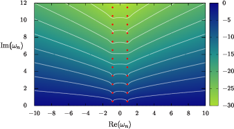
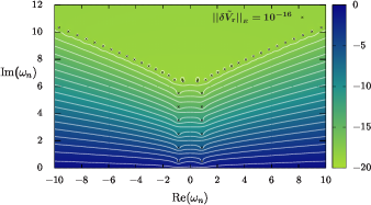
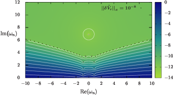
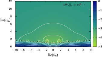
  Figure 1: Pseudospectrum regularization and evolution timescales. White lines correspond to contour lines of $\epsilon$-pseudospectra, with $\epsilon$ growing towards the dark green regions (i.e. downwards in the figure). High wave-number (random) perturbations of size $\epsilon_{o}=||\delta\tilde{V}||_{E}$ flatten the pseudospectrum (namely, regularize the resolvent $R_{L}(z)$) for $\epsilon<\epsilon_{o}$, therefore modifying the dynamics for $t_{\epsilon}>t_{\epsilon_{o}}$. Pseudospectra lines for $\epsilon>\epsilon_{o}$ remain however unaltered, indicating that early dynamics with $t_{\epsilon}<t_{\epsilon_{o}}$ are not affected by these perturbations.

• Pseudospectrum regularization and $\epsilon$-dual QNM expansions. In ref. [31] the notion of ‘$\epsilon$-dual QNM expansions’ is introduced, based on the ‘stability’ (in the energy norm) of the time evolution, in contrast with the spectral QNM instability. In brief, considering the evolution operator $L(x)$ in a stationary spacetime and the stationary perturbation $\delta L(x)$ giving rise to the perturbed evolution operator $L^{\epsilon}=L+\epsilon\delta L$ (with $||\delta L||=1$), the respective (right-)spectral problems obtained under Fourier transform of (28) in time are

  $$L\hat{v}_{n}=\omega_{n}\hat{v}_{n}\quad,\quad L^{\epsilon}\hat{v}^{\epsilon}_{n}(x)=\omega^{\epsilon}_{n}\hat{v}^{\epsilon}_{n}(x)\ .$$ (56)

  Then, it is shown [31] that the corresponding unperturbed and perturbed evolution fields, $u(\tau,x)$ and $u^{\epsilon}(\tau,x)$, admit natural (Keldysh) QNM-resonant asymptotic expansions in the respective unperturbed and perturbed QNM frequencies and eigenfunctions

  $$u(\tau,x)\sim\sum_{n}e^{i\omega_{n}\tau}a_{n}\hat{v}_{n}(x)\quad,\quad u^{\epsilon}(\tau,x)\sim\sum_{n}e^{i\omega^{\epsilon}_{n}\tau}a^{\epsilon}_{n}\hat{v}^{\epsilon}_{n}(x)\ .$$ (57)

  From the (energy norm) stability of the time evolution, it holds $||u-u^{\epsilon}||_{{}_{E}}\ \lesssim C\epsilon$, so we can write $u^{\epsilon}(\tau,x)\sim u(\tau,x)+O(\epsilon)$. The associated QNM expansions cannot be distinguished at order $\epsilon$ and are therefore equivalent at order $\epsilon$, something we write [31]

  $$\sum_{n}e^{i\omega^{\epsilon}_{n}\tau}a^{\epsilon}_{n}\hat{v}^{\epsilon}_{n}(x)\stackrel{{\scriptstyle\epsilon}}{{\sim}}\sum_{n}e^{i\omega_{n}\tau}a_{n}\hat{v}_{n}(x)\ .$$ (58)

  Both expansions are indistinguishable up to errors of order $\epsilon$, providing two alternative descriptions of the evolved field at this order . This picture is consistent with the above-discussed regularization of the pseudospectra by order $\epsilon_{o}$ perturbations: for early times (with $\epsilon\geq\epsilon_{o}$) the pseudospectra and associated time evolutions are indistinguishable, whereas for late times (with $\epsilon\leq\epsilon_{o}$) the description may differ. In other words, $\epsilon$-dual QNM expansions correspond to equivalent resonant expansions for early times, associated with the unperturbed part of the pseudospectrum under order-$\epsilon_{o}$ perturbations.

• Non-stationary perturbations and time averaging. The non-perturbed and perturbed QNM problems in Eq. (56) assume the stationarity of the operator $L$ and the perturbation $\delta L$. The same holds for the problems studied in [50, 51, 31, 26] and, more generally, the stationarity hypothesis pervades the standard approach to the very definition of QNMs . Whereas the stationarity of $L$ is a reasonable hypothesis due to the uniqueness BH theorems, the stationarity of the perturbation $\delta L$ is a strong physical hypothesis. If we rather consider the evolution problem under a time-dependent perturbation $\delta L(\tau,x)$

  $$\partial_{\tau}u^{\epsilon}(\tau,x)=\big{(}L(x)+\epsilon\delta L(\tau,x)\big{)}u^{\epsilon}(\tau,x)\ ,$$ (59)

  a natural approximation approach (in particular, for oscillating $\delta L(\tau,x)$’s of period $T$) is to adopt an averaging method (e.g. [67, 58]) to set a time-independent problem

  $$\!\!\!\!\!\!\!\!\!\!\!\!\!\!\!\!\!\!\partial_{\tau}\bar{u}^{\epsilon}(\tau,x)=\big{(}L(x)+\epsilon\overline{\delta L}(x)\big{)}\bar{u}^{\epsilon}(\tau,x)\ \ ,\ \ \overline{\delta L}(x)=\frac{1}{T}\int_{0}^{T}\delta L(t,x)d\tau\ ,$$ (60)

  where the difference between $u^{\epsilon}$ and the averaged $\bar{u}^{\epsilon}$ is bounded in the time $\tau$, by

  $$||u^{\epsilon}-\bar{u}^{\epsilon}||(\tau)<C\epsilon\ ,$$ (61)

  with $\tau$ in the interval $\tau\!\in]0,\frac{\tau_{0}}{\epsilon}[$, for some constants $C$ and $\tau_{0}$. This has direct implications in our spectral BH QNM spectral instability problem. In particular, if we consider an oscillating perturbation averaging to zero in time, i.e. $\overline{\delta L}(x)=0$ (as it is indeed reasonable to assume for numerical noise in BBH simulations), the averaged signal $\bar{u}^{\epsilon}(\tau,x)$ corresponds actually to the non-perturbed signal $u(\tau,x)$ in the non-perturbed problem. Only if we go to time-samplings below the period $T$ of the oscillation, i.e. if we consider $\tau_{0}/\epsilon$ sufficiently small and therefore with an $\epsilon$ in (61) large enough, would the averaged signal depart from the unperturbed one. This mechanism seems to be adequate to explain the absence of observed departures from the expected, non-perturbed results, in BBH numerical simulations. Regarding actual astrophysical observational data, if the sampling of the time-series for the ringdown signal is coarser that the period of the (potential) astrophysical perturbations and the latter average to zero over such timescales, again, we would retrieve unperturbed QNMs from the ringdown signal. This poses a challenging technological problem to retrieve fastly oscillating astrophysical sources.

4 A unifying effective linear-dynamics approach to BBH dynamical phases

In these notes we have proposed the pseudospectrum notion and the related non-modal analysis as a framework to study the BBH merger waveform as a transient phenomenon, under the (strong) hypothesis of effective BBH non-normal linear dynamics. This approach provides a unified scheme to study the different phases of the BBH waveform in terms of $\epsilon$-pseudospectra, the (late) inspiral phase corresponding to the limit $\epsilon\to\infty$, the final ringdown characterised by $\epsilon\to 0$ and the actual merger by intermediate values of $\epsilon$. In particular, qualitative insights gained from such unified pseudospectrum perspective may provide clues in the effort to understand the simplicity and universality of BBH merger waveforms [46, 47].

Specifically, given the infinitesimal dynamical time generator $L$, we have introduced: i) the numerical abscissa $\omega(L)$, controlling the triggering of the dynamical transient, ii) the pseudospectral abscissa $\alpha_{\epsilon}(L)$ and the Kreiss constant ${\cal K}(L)$ offering estimates of the transient peak, and iii) the spectral abscissa $\alpha(L)$ (or spectral gap) controlling the late time behaviour. We have endowed the $\epsilon$ parameter in $\epsilon$-pseudospectra with an interpretation as an inverse dynamical timescale, namely $t_{\mathrm{dyn}}\sim t_{\epsilon}\sim 1/\epsilon$, in such a way that non-trivial patterns in the $\epsilon$-contour lines of the pseudospectrum qualitatively inform of dynamical processes occurring at the $t_{\epsilon}$ timescale. In particular, as a consequence of the asymptotic universality of the pseudospectrum at large $\epsilon$’s, we have concluded that early BBH merger waveforms are largely independent of possible (environmental) perturbations in the BBH dynamics, deviations only appearing at late times controlled by the spectrum, i.e. encoded in possibly perturbed QNMs.

Concerning the latter context of perturbations in (after merger) BBH dynamics, namely the question of BH QNM spectral instability, we have discussed the following refinements: i) perturbations with ‘energy’ of order $\Delta E$ only affect post-merger dynamics in timecales larger than a $\Delta t$ constrained by $\Delta E\cdot\Delta t\geq({\cal K}(L))^{-1}$, ii) ‘$\epsilon$-dual’ QNM expansions associated with non-perturbed and perturbed QNMs provide equivalent resonant expansions for early times $t\leq t_{\epsilon}$, and iii) non-stationary perturbations averaging to zero in a timescale $T$ render exactly the non-perturbed BH QNMs (in spite of the BH QNM spectral instability phenomenon) if the sampling-time of the signal is larger than $T$, QNM instabilities only becoming apparent for finer time samplings. The latter point is crucial for assessing time-varying BH perturbations.

The present notes must be understood as an introductory invitation to the subject, aiming at prompting a deeper and systematic application of non-modal analysis (e.g. [80, 79, 81, 28, 77, 23, 24, 74, 76]), well-established in the hydrodynamics context, to the gravitational setting and, in particular, to the BBH problem. As an illustration, the non-modal analysis tools specifically discussed here have been implemented in the particular instance provided by the ‘close limit’ approximation to BBH dynamics. Specifically, a fully explicit calculation of the numerical abscissa $\omega(L)$ (and also of the Kreiss constant ${\cal K}(L)$) has been presented, making use of a compactified hyperboloidal approach to linear dynamics over a Schwarzschild background. The conclusion is that the BBH merger peak cannot be accounted in such ‘close limit’ approximation, therefore this particular Ansatz for the effective BBH linear dynamics does not provide a good modelling of the dynamical transient from the inspiral to the merger phases. At the first-order in perturbation theory, this follows from the vanishing of the numerical abscissa, namely $\omega(L)=0$. At the same time, this very result supports the validity of the ‘close limit’ in the dynamics starting at the peak of the merger. Even if we go to second-order perturbation theory, the ‘close limit’ approximation does not provide a good account of the transient peak, as shown in the A, where the pseudospectrum is used to assess the possibility of understanding the merger peak in terms of a so-called ‘pseudo-resonance’, but without success (the ‘pseudo-resonance’ concept can be however useful on other (ultra-)compact object settings, as explored in [13]). The bottomline of this ‘close-limit’ approximation analysis is that a refined model is needed to explore the effective linear dynamics hypothesis, the key point being —as indicated in section 1— the correct identification of the relevant background dynamics. This is precisely the goal in [47].

Addressing this latter point from a more general perspective, in these notes we have discussed the possibility of studying the BBH merger process as a dynamical transient described by the (non-normal) linear dynamics for some (fast) degrees of freedom $u$ determined by the initial data problem (3) or, in the notation in [50], by the equation (28). As indicated in the introductory section 1, this is a bold assumption in the setting of a non-linear theory such as general relativity. Even more, it is in manifest tension with sound approaches to the BBH merger problem that vindicate precisely the key role of non-linearities [73]. Our approach in this sense is an ‘agnostic’ one open to intermediate effective treatments integrating both linear and genuinely non-linear mechanisms, each one addressing distinct but concurrent phenomena. An example of this is provided in the study of hydrodynamical instability and turbulence, where linear non-normal transient growths can indeed act as the seed triggering the full development of the non-linear turbulent regime [80, 74], in a kind of ‘bootstrapping’ mechanism. Specifically in our gravitational setting, the present discussion has focused on the effective linear dynamics of fields $u$ propagating on a (fixed) background determined by the dynamical time operator $L$. A natural further step would consist in endowing $L$ with genuine (effective) non-linear dynamics corresponding to (slow) background degrees of freedom, very much in the spirit of ‘wave-mean flow’ approaches in hydrodynamics [14]. In this context, the present pseudospectrum transient discussion is a part of a more ambitious program aiming at understanding the qualitative mechanisms of BBH dynamics, in particular the simplicity and universality of BBH merger waveforms [46, 47].

Appendix A Pseudospectrum and pseudo-resonances: assessing the BBH merger peak

In the spirit of integrating both linear and genuinely non-linear mechanisms in BBH dynamics, we consider in this appendix another important aspect of the pseudospectrum that may be of relevance when incorporating general relativistic non-linear effects in a higher-order perturbation scheme . Our non-modal analysis discussion has been based on the capability of the pseudospectrum to explain transients in non-normal initial value problems, without external forcing. However, the pseudospectrum is also relevant to account for dynamical effects when the non-normal linear system is driven by an external force, leading to the notion of ‘pseudo-resonance’: enhanced resonant responses to external forces, not related to the QNM spectrum, occurring when $\epsilon$-pseudospectra reach large values far from the spectrum. In our BBH context, the external forcing is precisely given by second-order perturbation theory.

General relativity perturbation theory is a delicate subject plenty of subtle conceptual and technical points. Here we dwell at a purely formal level, interested in the resulting hierarchy of linear equations at different orders, with a focus on the second order. Following [40, 21] (see also [55, 68] for the specific notation), we expand the metric $g_{ab}$ to second order as

$$g_{ab}=g^{(0)}_{ab}+\epsilon h^{(1)}_{ab}+\epsilon^{2}h^{(2)}_{ab}+O(\epsilon^{3})\ .$$ (62)

Adopting gauges such that perturbed (vacuum) Einstein equations to second order write as

$$\delta G_{ab}\cdot h^{(1)} = 0$$

$$\delta G_{ab}\cdot h^{(2)} = \delta^{2}G_{ab}[h^{(1)},h^{(1)}]\ ,$$ (63)

where $\delta G_{ab}$ is the linearized Einstein tensor evaluated on $g^{(0)}_{ab}$ acting linearly on $h^{(1)}_{ab}$ and $h^{(2)}_{ab}$, respectively at first and second-perturbation order (we use the notation “$\cdot$” to emphasize the linear action). Then $\delta^{2}G_{ab}[h^{(1)},h^{(1)}]$ is the second-order variation of the Einstein tensor evaluated on the first-order metric perturbation (having a formal structure $\delta^{2}G\sim h^{(1)}\partial^{2}h^{(1)}+\partial h^{(1)}\partial h^{(1)}$). In summary, we have a hierarchy of linear equations crucially sharing the same left-hand side, given by differential linear operator $\delta G_{ab}$ corresponding to the non-perturbed metric, and with right-hand side sources determined at each order by lower-order solutions . In vacuum, the first-order in this hierarchy is a homogeneous equation.

Having sketched the general relativistic perturbation setting, we revisit now the close-limit approximation to BBH mergers. Specifically, in section 3 of the main text we have addressed the close-limit approximation through its formulation relying on the general relativity perturbation theory at first-order [72]. We have seen that this approximation does not account for the transition from the late inspiral to the merger phase and, in particular, for the merger peak. However, the close-limit approximation can be upgraded to an improved version at second-order in perturbation theory [33]. Specifically, Eqs. (A) can be cast as [33, 21]

$$\left(\partial_{\tau}-iL\right)u^{(1)} = 0$$

$$\left(\partial_{\tau}-iL\right)u^{(2)} = S(\tau,x;u^{(1)})\ ,$$ (64)

where we have used again the notation in [50], with $L$ the evolution operator in Eqs. (31) and (32) fixed by the non-perturbed Schwarzschild spacetime. The first-order (homogeneous) equation, corresponds to the evolution Eq. (28) in the transient (initial data) scheme discussed in section 3. In the second-order equation, the source $S(\tau,x;u^{(1)})$ would be fixed in terms of the first-order perturbation $u^{(1)}$. For simplicity, we write it in the following as $S(\tau,x)$.

Following [80, 74] let us consider for simplicity a monochromatic harmonic forcing

$$S(\tau,x)=e^{i\omega\tau}s(x)\ ,$$ (65)

with $\omega\in\mathbb{C}$. We can then solve the inhomogeneous second equation in (A) by acting with the resolvent $R_{L}(\omega)$ (essentially the Green’s function of $(\omega I-L)$) on the source $S(\tau,x)$

$$u^{(2)}(\tau,x)=\frac{1}{i}e^{i\omega\tau}\big{(}(\omega-L)^{-1}s\big{)}(x)=\frac{1}{i}e^{i\omega\tau}\big{(}R_{L}(\omega)s\big{)}(x)\ .$$ (66)

At this point, we can evaluate the maximum response $R_{\mathrm{max}}$ we can get in this forced system by maximizing the ratio between the norm of $u^{(2)}$ and that of all possible sources $s$, namely

$$\!\!\!\!\!\!\!\!\!\!\!\!\!\!\!\!\!\!\!\!\!\!\!\!\!\!\!\!\!\!\!\!\!\!\!\!\!\!\!\!\!\!\!R_{\mathrm{max}}(\omega)=\sup_{s\neq 0}\frac{||u^{(2)}||}{||s||}=e^{-\mathrm{Im}(\omega)\tau}\sup_{s\neq 0}\frac{||(\omega-L)^{-1}s||}{||s||}=e^{-\mathrm{Im}(\omega)\tau}||(\omega-L)^{-1}||$$

$$\!\!\!\!\!\!\!\!\!\!\!\!\!\!\!\!\!\!\!=e^{-\mathrm{Im}(\omega)\tau}||R_{L}(\omega)||\ ,$$ (67)

where we have used the induced operator norm to express the response $R_{\mathrm{max}}(\omega)$ in terms of the (induced) norm of the resolvent of $L$. This describes a resonant phenomenon: when the frequency $\omega$ falls onto the spectrum $\sigma(L)$ of $L$, the response $R_{\mathrm{max}}(\omega)$ diverges, characterizing a resonance of the system. If $L$ is a normal operator, $||R_{L}(\omega)||\leq 1/\mathrm{dist}(\omega,\sigma(L))$, decreasing fast when moving away from the spectrum of $L$ and no more resonant phenomena occur.

The situation changes if $L$ is a non-normal operator. Indeed, Eq. (A) makes direct contact with the $\epsilon$-pseudospectrum notion through its first characterization in (iii)). If $L$ is a non-normal operator then $||R_{L}(\omega)||$ can get very large, therefore describing a resonant behaviour, even if $\omega$ is far from the spectrum $\sigma(L)$: this characterizes $\omega$ as a pseudo-resonance.

The interest of the harmonic source (65) is that any (appropriate) time-dependent source $S(\tau,x)$ can be written as a continuous superposition of harmonic sources (65) with real $\omega$’s through a standard Fourier transform. Maximizing then $R_{\mathrm{max}}(\omega)$ in (A) over all $\omega\in\mathbb{R}$

$$R_{\mathrm{max}}=\sup_{\omega\in\mathbb{R}}R_{\mathrm{max}}(\omega)=\sup_{\omega\in\mathbb{R}}||(\omega-L)^{-1}||=\sup_{\omega\in\mathbb{R}}||R_{L}(\omega)||\ ,$$ (68)

we get the maximum possible response to a time-dependent forcing $S(\tau,x)$. Following [80], pseudospectra contour lines can then be seen as lines in the frequency-$\omega$ complex plane with the same resonance response magnitude. Therefore, is $\epsilon$-pseudospectra with small $\epsilon$ (therefore large $||R_{L}(\omega)||$) approach the real line, pseudo-resonant phenomena can be expected.

Finally, we can assess the capability of the close-limit approximation at the second-order in perturbation theory to account for the merger peak as a non-linear resonant phenomenon in which second-order perturbations would act as a forcing. This would require the pseudospectrum of Schwarzschild to present small $\epsilon$-pseudospectra sets approaching the real line. Since this turns out not to be case (cf. analysis in [50]) we can conclude that the second-order close-limit approximation does neither account for the merger peak: the close-limit approximation may apply from the merger, but not before . This resonant mechanism may, on the contrary, prove of interest in the dynamical instability of ultracompact objects [13].

References

- [1] B. P. Abbott et al., Observation of Gravitational Waves from a Binary Black Hole Merger, Phys. Rev. Lett. 116(6), 061102 (2016).
- [2] M. Ansorg & R. Panosso Macedo, Spectral decomposition of black-hole perturbations on hyperboloidal slices, Phys. Rev. D93(12), 124016 (2016).
- [3] A. Ashtekar, N. Khera, M. Kolanowski, & J. Lewandowski, Charges and fluxes on (perturbed) non-expanding horizons, JHEP 02, 066 (2022).
- [4] A. Ashtekar, N. Khera, M. Kolanowski, & J. Lewandowski, Non-expanding horizons: multipoles and the symmetry group, JHEP 01, 028 (2022).
- [5] V. Baibhav, E. Berti, V. Cardoso, & G. Khanna, Black hole spectroscopy: Systematic errors and ringdown energy estimates, Physical Review D 97(4) (Feb 2018).
- [6] J. G. Baker, B. Bruegmann, M. Campanelli, C. O. Lousto, & R. Takahashi, Plunge wave forms from inspiralling binary black holes, Phys. Rev. Lett. 87, 121103 (2001).
- [7] J. G. Baker, M. Campanelli, & C. O. Lousto, The Lazarus project: A Pragmatic approach to binary black hole evolutions, Phys. Rev. D 65, 044001 (2002).
- [8] E. Berti, V. Cardoso, & C. M. Will, On gravitational-wave spectroscopy of massive black holes with the space interferometer LISA, Phys. Rev. D73, 064030 (2006).
- [9] D. Bindel & M. Zworski, Theory and computation of resonances in 1d scattering. http://www.cs.cornell.edu/%7Ebindel/cims/resonant1d/
- [10] W. Bordeaux Montrieux, Loi de Weyl presque sûre et résolvante pour des opérateurs non-autoadjoints, Theses, Ecole Polytechnique X (2008).
- [11] W. Bordeaux Montrieux, Almost sure Weyl law for a differential system in dimension 1, Annales Henri Poincaré 1 (01 2011).
- [12] S. Borhanian, K. G. Arun, H. P. Pfeiffer, & B. S. Sathyaprakash, Comparison of post-Newtonian mode amplitudes with numerical relativity simulations of binary black holes, Class. Quant. Grav. 37(6), 065006 (2020).
- [13] V. Boyanov, K. Destounis, J. L. Jaramillo, R. P. Macedo, & V. Cardoso, Pseudospectrum of horizonless compact objects: a bootstrap instability mechanism, In preparation (2022).
- [14] O. Bühler, Waves and Mean Flows, Cambridge Monographs on Mechanics, Cambridge University Press, 2 edition (2014).
- [15] A. Buonanno & T. Damour, Effective one-body approach to general relativistic two-body dynamics, Phys. Rev. D 59, 084006 (1999).
- [16] A. Buonanno & T. Damour, Transition from inspiral to plunge in binary black hole coalescences, Phys. Rev. D 62, 064015 (2000).
- [17] M. Cabero, J. Westerweck, C. D. Capano, S. Kumar, A. B. Nielsen, & B. Krishnan, The next decade of black hole spectroscopy, Phys. Rev. D101(6), 064044 (2020).
- [18] C. D. Capano, M. Cabero, J. Westerweck, J. Abedi, S. Kastha, A. H. Nitz, A. B. Nielsen, & B. Krishnan, Observation of a multimode quasi-normal spectrum from a perturbed black hole, 5 (2021).
- [19] M. H.-Y. Cheung, K. Destounis, R. P. Macedo, E. Berti, & V. Cardoso, The elephant and the flea: destabilizing the fundamental mode of black holes, (11 2021).
- [20] R. Cotesta, G. Carullo, E. Berti, & V. Cardoso, On the detection of ringdown overtones in GW150914, arXiv:2201.00822 (2022).
- [21] C. T. Cunningham, R. H. Price, & V. Moncrief, Radiation from collapsing relativistic stars. III - Second order perturbations of collapse with rotation, Astrophysical Journal 236, 674–692 (Mar. 1980).
- [22] T. Damour, The problem of motion in Newtonian and Einsteinian gravity, Three Hundred Years of Gravitation, pages 128–198, eds. Hawking, S.W. and Israel, W. Cambridge University Press (1989).
- [23] E. Davies, Semigroup growth bounds, Journal of Operator Theory , 225–249 (2005).
- [24] E. Davies, Linear Operators and their Spectra, Cambridge Studies in Advanced Mathematics, Cambridge University Press (2007).
- [25] M. Davis, R. Ruffini, W. H. Press, & R. H. Price, Gravitational Radiation from a Particle Falling Radially into a Schwarzschild Black Hole, Phys. Rev. Lett. 27, 1466–1469 (Nov 1971).
- [26] K. Destounis, R. P. Macedo, E. Berti, V. Cardoso, & J. L. Jaramillo, Pseudospectrum of Reissner-Nordström black holes: Quasinormal mode instability and universality, Phys. Rev. D 104(8), 084091 (2021).
- [27] O. Dreyer, B. J. Kelly, B. Krishnan, L. S. Finn, D. Garrison, & R. Lopez-Aleman, Black hole spectroscopy: Testing general relativity through gravitational wave observations, Class. Quant. Grav. 21, 787–804 (2004).
- [28] M. Embree & N. Trefethen, https://www.cs.ox.ac.uk/pseudospectra/index.html (Personal Website).
- [29] E. Finch & C. J. Moore, Searching for a Ringdown Overtone in GW150914, arXiv:2205.07809 (2022).
- [30] X. J. Forteza & P. Mourier, High-overtone fits to numerical relativity ringdowns: Beyond the dismissed n=8 special tone, Phys. Rev. D 104(12), 124072 (2021).
- [31] E. Gasperin & J. L. Jaramillo, Energy scales and black hole pseudospectra: the structural role of the scalar product, Class. Quant. Grav. 39(11), 115010 (2022).
- [32] M. Giesler, M. Isi, M. A. Scheel, & S. Teukolsky, Black Hole Ringdown: The Importance of Overtones, Phys. Rev. X9(4), 041060 (2019).
- [33] R. J. Gleiser, C. O. Nicasio, R. H. Price, & J. Pullin, Colliding black holes: How far can the close approximation go?, Phys. Rev. Lett. 77, 4483–4486 (1996).
- [34] A. Gupta, B. Krishnan, A. Nielsen, & E. Schnetter, Dynamics of marginally trapped surfaces in a binary black hole merger: Growth and approach to equilibrium, Phys. Rev. D97(8), 084028 (2018).
- [35] M. Hager, Instabilite spectrale semiclassique d’operateurs non-autoadjoints, Theses, Ecole Polytechnique X, June 2005, Jury: Bony Jean-Michel, Dimassi Mouez, Helffer Bernard, Lerner Nicolas, Zworski Maciej (2005).
- [36] M. Hager, Instabilité spectrale semiclassique d’opérateurs non-autoadjoints. II, Ann. Henri Poincaré 7(6), 1035–1064 (2006).
- [37] M. Hager, Instabilité spectrale semiclassique pour des opérateurs non-autoadjoints. I: un modèle, Ann. Fac. Sci. Toulouse, Math. (6) 15(2), 243–280 (2006).
- [38] M. Hager & J. Sjöstrand, Eigenvalue asymptotics for randomly perturbed non-selfadjoint operators, arXiv Mathematics e-prints , math/0601381 (Jan. 2006).
- [39] D. A. B. Iozzo et al., Comparing Remnant Properties from Horizon Data and Asymptotic Data in Numerical Relativity, Phys. Rev. D 103(12), 124029 (2021).
- [40] R. A. Isaacson, Gravitational Radiation in the Limit of High Frequency. I. The Linear Approximation and Geometrical Optics, Phys. Rev. 166, 1263–1271 (Feb 1968).
- [41] M. Isi & W. M. Farr, Revisiting the ringdown of GW150914, arXiv:2202.02941 (2022).
- [42] M. Isi, W. M. Farr, M. Giesler, M. A. Scheel, & S. A. Teukolsky, Testing the Black-Hole Area Law with GW150914, Phys. Rev. Lett. 127(1), 011103 (2021).
- [43] M. Isi, M. Giesler, W. M. Farr, M. A. Scheel, & S. A. Teukolsky, Testing the no-hair theorem with GW150914, Phys. Rev. Lett. 123(11), 111102 (2019).
- [44] J. Jaramillo, R. Macedo, P. Moesta, & L. Rezzolla, Towards a cross-correlation approach to strong-field dynamics in Black Hole spacetimes, AIP Conf.Proc. 1458, 158–173 (2011).
- [45] J. L. Jaramillo, An introduction to local Black Hole horizons in the 3+1 approach to General Relativity, International Journal of Modern Physics 20, 2169–2204 (2011).
- [46] J. L. Jaramillo & B. Krishnan, Airy-function approach to binary black hole merger waveforms: The fold-caustic diffraction model, arXiv:2206.02117 (2022).
- [47] J. L. Jaramillo & B. Krishnan, Painlevé-II approach to binary black hole merger dynamics: universality from integrability, In preparation.
- [48] J. L. Jaramillo, R. P. Macedo, P. Moesta, & L. Rezzolla, Black-hole horizons as probes of black-hole dynamics II: geometrical insights, Phys.Rev. D85, 084031 (2012).
- [49] J. L. Jaramillo, R. P. Macedo, P. Moesta, & L. Rezzolla, Black-hole horizons as probes of black-hole dynamics I: post-merger recoil in head-on collisions, Phys.Rev. D85, 084030 (2012).
- [50] J. L. Jaramillo, R. Panosso Macedo, & L. Al Sheikh, Pseudospectrum and Black Hole Quasinormal Mode Instability, Phys. Rev. X 11(3), 031003 (2021).
- [51] J. L. Jaramillo, R. Panosso Macedo, & L. A. Sheikh, Gravitational Wave Signatures of Black Hole Quasinormal Mode Instability, Phys. Rev. Lett. 128(21), 211102 (2022).
- [52] G. Khanna, J. G. Baker, R. J. Gleiser, P. Laguna, C. O. Nicasio, H.-P. Nollert, R. Price, & J. Pullin, Inspiralling black holes: The Close limit, Phys. Rev. Lett. 83, 3581–3584 (1999).
- [53] P. D. Lax & R. S. Phillips, Scattering theory, volume 26 of Pure and Applied Mathematics, Academic Press, Boston, second edition edition (1989).
- [54] E. Maggio, L. Buoninfante, A. Mazumdar, & P. Pani, How does a dark compact object ringdown?, Phys. Rev. D 102(6), 064053 (2020).
- [55] J. Miller, B. Wardell, & A. Pound, Second-order perturbation theory: the problem of infinite mode coupling, Phys. Rev. D 94(10), 104018 (2016).
- [56] W. B. Montrieux, Estimation de résolvante et construction de quasimode près du bord du pseudospectre, arXiv:1301.3102 (2013).
- [57] W. B. Montrieux & J. Sjöstrand, Almost sure Weyl asymptotics for non-self-adjoint elliptic operators on compact manifolds, Ann. Fac. Sci. Toulouse, Math. (6) 19(3-4), 567–587 (2010).
- [58] J. A. Murdock, Perturbations: theory and methods, SIAM (1999).
- [59] S. Nonnenmacher & M. Vogel, Local eigenvalue statistics of one-dimensional random non-selfadjoint pseudo-differential operators, arXiv:1711.05850 (2018).
- [60] M. Okounkova, Revisiting non-linearity in binary black hole mergers, arXiv:2004.00671 (2020).
- [61] I. Ota & C. Chirenti, Overtones or higher harmonics? Prospects for testing the no-hair theorem with gravitational wave detections, Phys. Rev. D 101(10), 104005 (2020).
- [62] I. Ota & C. Chirenti, Black hole spectroscopy horizons for current and future gravitational wave detectors, arXiv:2108.01774 (2021).
- [63] R. Panosso Macedo, Comment on “Some exact quasinormal frequencies of a massless scalar field in Schwarzschild spacetime”, Phys. Rev. D99(8), 088501 (2019).
- [64] R. Panosso Macedo, Hyperboloidal framework for the Kerr spacetime, Class. Quant. Grav. 37(6), 065019 (2020).
- [65] R. Panosso Macedo & M. Ansorg, Axisymmetric fully spectral code for hyperbolic equations, J. Comput. Phys. 276, 357–379 (2014).
- [66] R. Panosso Macedo, J. L. Jaramillo, & M. Ansorg, Hyperboloidal slicing approach to quasi-normal mode expansions: the Reissner-Nordström case, Phys. Rev. D98(12), 124005 (2018).
- [67] L. M. Perko, Higher Order Averaging and Related Methods for Perturbed Periodic and Quasi-Periodic Systems, SIAM Journal on Applied Mathematics 17(4), 698–724 (1969).
- [68] A. Pound, Gauge and motion in perturbation theory, Phys. Rev. D 92(4), 044021 (2015).
- [69] V. Prasad, A. Gupta, S. Bose, B. Krishnan, & E. Schnetter, News from horizons in binary black hole mergers, arXiv:2003.06215 (2020),
- [70] F. Pretorius, Evolution of Binary Black-Hole Spacetimes, Phys. Rev. Lett. 95, 121101 (2005).
- [71] F. Pretorius, Binary Black Hole Coalescence, arXiv:0710.1338 (2007).
- [72] R. H. Price & J. Pullin, Colliding black holes: The Close limit, Phys. Rev. Lett. 72, 3297–3300 (1994).
- [73] L. Sberna, P. Bosch, W. E. East, S. R. Green, & L. Lehner, Nonlinear effects in the black hole ringdown: Absorption-induced mode excitation, Phys. Rev. D 105(6), 064046 (2022).
- [74] P. J. Schmid, Nonmodal Stability Theory, Annual Review of Fluid Mechanics 39(1), 129–162 (2007).
- [75] B. F. Schutz, The Art and science of black hole mergers, in Conference on Growing Black Holes: Accretion in a Cosmological Context, gr-qc/0410121 (2004).
- [76] J. Sjöstrand, Non-Self-Adjoint Differential Operators, Spectral Asymptotics and Random Perturbations, Pseudo-Differential Operators, Springer International Publishing, 2019.
- [77] J. Sjöstrand, Pseudospectrum for differential operators, Sémin. Équ. Dériv. Partielles, Éc. Polytech., Cent. Math. Laurent Schwartz, Palaiseau 2002-2003, ex (2003).
- [78] A. Soffer & M. I. Weinstein, Time dependent resonance theory, Geometric & Functional Analysis GAFA 8(6), 1086–1128 (1998).
- [79] L. N. Trefethen, Pseudospectra of linear operators, SIAM Rev. 39(3), 383–406 (1997).
- [80] L. N. Trefethen, A. E. Trefethen, S. C. Reddy, & T. A. Driscoll, Hydrodynamic Stability Without Eigenvalues, Science 261(5121), 578–584 (1993).
- [81] L. Trefethen & M. Embree, Spectra and Pseudospectra: The Behavior of Nonnormal Matrices and Operators, Princeton University Press (2005).
- [82] M. Vogel, Spectral statistics of non-selfadjoint operators subject to small random perturbations, Séminaire Laurent Schwartz — EDP et applications (2016-2017), talk:19.
- [83] A. Zenginoglu, Hyperboloidal foliations and scri-fixing, Class. Quant. Grav. 25, 145002 (2008).
- [84] A. Zenginoglu, A Geometric framework for black hole perturbations, Phys. Rev. D83, 127502 (2011).
- [85] M. Zworski, Mathematical study of scattering resonances, Bulletin of Mathematical Sciences 7(1), 1–85 (2017).