On Error and Compression Rates for Prototype Rules

Abstract

We study the close interplay between error and compression in the non-parametric multiclass classification setting in terms of prototype learning rules. We focus in particular on a recently proposed compression-based learning rule termed OptiNet (Kontorovich, Sabato, and Urner 2016; Kontorovich, Sabato, and Weiss 2017; Hanneke et al. 2021). Beyond its computational merits, this rule has been recently shown to be universally consistent in any metric instance space that admits a universally consistent rule—the first learning algorithm known to enjoy this property. However, its error and compression rates have been left open. Here we derive such rates in the case where instances reside in Euclidean space under commonly posed smoothness and tail conditions on the data distribution. We first show that OptiNet achieves non-trivial compression rates while enjoying near minimax-optimal error rates. We then proceed to study a novel general compression scheme for further compressing prototype rules that locally adapts to the noise level without sacrificing accuracy. Applying it to OptiNet, we show that under a geometric margin condition, further gain in the compression rate is achieved. Experimental results comparing the performance of the various methods are presented.

Introduction

The interplay between learning and compression has long been recognized, popularized by Occam’s razor rule of thumb (Ariew 1976), and rigorously studied in several frameworks, including in information theory in terms of the minimum description length principal and Kolmogorov complexity (Cover 1999; Li, Vitányi et al. 2008), and more recently in terms of sample compression schemes in the PAC statistical learning framework (Littlestone and Warmuth 1986; Floyd and Warmuth 1995; Graepel, Herbrich, and Shawe-Taylor 2005; Gottlieb, Kontorovich, and Nisnevitch 2014; David, Moran, and Yehudayoff 2016; Hanneke and Kontorovich 2019; Hanneke, Kontorovich, and Sadigurschi 2019; Bousquet et al. 2020; Hanneke and Kontorovich 2021; Alon et al. 2021).

Consider for example the well-known support vector machine (SVM) (Vapnik 2013). Given a binary labeled dataset, SVM retains only the samples constituting the support vectors. In the linearly realizable case—where a hyperplane discriminator can achieve zero population error—the number of support vectors can be taken to be at most $d$, leading to ultrafast optimal error and compression rates of order $O(d/n)$, where $d$ is the dimension of the instance space ${\mathbb{R}}^{d}$ and $n$ is the number of independent labeled samples in the dataset. More generally in the parametric setting, similar optimal rates are achieved when one can construct a stable compression scheme of size $d$ that is guaranteed to obtain zero sample error for all $n$ while retaining only up to $d$ samples (Bousquet et al. 2020).

In the more general non-parametric setting, however, it is well known that for any learning rule, the rate at which its error converges to the optimal one can be arbitrarily slow without further assumptions on the data distribution (Devroye, Györfi, and Lugosi 1996). The same holds for the achievable sample compression rates of accurate rules. Results on the jointly achievable error and compression rates in the non-parametric setting in terms of the properties of the data distribution and the instance space are scarce and still not well understood. Here we aim at narrowing this gap.

Prototype learning rules.

A large family of non-parametric learning rules suitable for studying the error-compression interplay are prototype learning rules (Devroye, Györfi, and Lugosi 1996, Chapter 19). Such rules compress the data into a small number of prototypes and pair each prototype with a suitable label as computed from the dataset. A new instance is then labeled according to the label paired to its nearest prototype in the compressed dataset. The various prototype rules then differ in the way the prototypes and the paired labels are computed.

The simplest prototype rule is the 1-nearest-neighbor rule (1-NN) whose prototype-label set is simply the whole dataset. This rule, however, is known to be inconsistent in general—its error does not necessarily converge to the optimal one as the sample size grows. It is also known that the $k$-NN rule, which labels a new instance according to the label having the most counts among its $k$ nearest neighbors in the dataset, is consistent for any data distribution, provided $k\to\infty$ such that $k/n\to 0$. In other words, $k$-NN is universally consistent in ${\mathbb{R}}^{d}$ for any $d>0$ (Devroye, Györfi, and Lugosi 1996).

Beyond universal consistency, for several large families of data distributions, $k$-NN with a properly tuned $k$ achieves minimax optimal error rates—namely, the rate at which its error converges to the optimal one is also a lower bound for any other learning rule over the family of distributions under consideration. In particular, under the commonly posed $\beta$-Hölder smoothness condition on the labels’ conditional probabilities, the strong density condition on the instance marginal distribution, and the $\alpha$-Tsybakov margin condition that bounds the total mass of points having large noise, the $k$-NN rule with the choice $k\approx n^{{2\beta}/{(2\beta+d)}}$ achieves the minimax optimal error rate of order $n^{-{\beta(1+\alpha)}/{(2\beta+d)}}$ (Audibert and Tsybakov 2007; Chaudhuri and Dasgupta 2014; Gadat, Klein, and Marteau 2016).

While the $k$-NN rule does not attempt to compress the dataset, it has been recently shown by Xue and Kpotufe (2018) and Györfi and Weiss (2021) that a natural prototype version of $k$-NN still enjoys the same optimal error rates as $k$-NN while retaining only $m=O(n/k)$ prototypes from the dataset (see also Biau and Devroye (2010) for results in the same spirit). This rule, termed Proto-$k$-NN, randomly draws $m\approx n/k$ prototypes from the dataset and pairs each prototype with the label having the most counts among its $k$ nearest neighbors in the original dataset. Notably, with $k\approx n^{{2\beta}/{(2\beta+d)}}$ as above, the compression rate satisfies $m/n\approx n^{-{2\beta}/{(2\beta+d)}}\xrightarrow[]{n\to\infty}0$ while still enjoying the minimax error rate of order $n^{-{\beta(1+\alpha)}/{(2\beta+d)}}$.

Another simple prototype rule is Proto-NN (Györfi and Weiss 2021). Similarly to Proto-$k$-NN, this rule randomly draws $m\ll n$ prototypes from the dataset, but pairs each prototype with the label having the most counts among the samples from the dataset that fell into its Voronoi cell as determined by the other prototypes. While at first glance it may seem that Proto-NN and Proto-$k$-NN should behave similarly, it has been recently established by Györfi and Weiss (2021) that, in contrast to $k$-NN and Proto-$k$-NN, Proto-NN is universally consistent in any metric space admitting a universally consistent learning rule, including many important infinite-dimensional metric spaces for which $k$-NN and Proto-$k$-NN fail to be consistent (Cérou and Guyader 2006; Györfi and Weiss 2021). Chronologically, Proto-NN was derived as a simplification of OptiNet, a prototype rule that was first introduced in Kontorovich, Sabato, and Urner (2016), further studied in Kontorovich, Sabato, and Weiss (2017), and eventually shown in Hanneke et al. (2021) to be the first algorithm known to be universally consistent in any metric space that admits such a rule. However, the error and compression rates for the Voronoi partition-based rules Proto-NN and OptiNet were left open.

Main contributions.

In this paper we continue the study of error and compression rates for prototype rules and focus on OptiNet for the case where instances reside in the familiar Euclidean space. OptiNet selects its prototypes by computing a $\gamma$-net over the dataset for an appropriately tuned margin $\gamma>0$ and, similarly to Proto-NN, pairs each prototype with the label having the most counts among the samples that fell into its Voronoi cell.

As our first main contribution, we establish both theoretically and empirically that OptiNet achieves minimax optimal error rates under the aforementioned smoothness, margin, and tail conditions, while enjoying compression rates similar to those obtained for Proto-$k$-NN in Xue and Kpotufe (2018) and (Györfi and Weiss 2021), and in some cases even faster rates. In fact, as established by Gottlieb, Kontorovich, and Nisnevitch (2014); Chitnis (2022), OptiNet achieves near-optimal compression rates in the sense that further compressing the dataset while remaining consistent on the dataset is an NP-hard problem.

Next, notably, the compression rate $m/n\approx n^{-{2\beta}/{(2\beta+d)}}$ derived for Proto-$k$-NN, as well as those derived for OptiNet in this paper, are insensitive to the Tsybakov noise parameter $\alpha$ that restricts the mass of points having high noise level. This stems from the fact that these rules do not attempt to focus their resources on the decision boundary where classification is harder. This approach was made practical by several adaptive learning algorithms, such as decision trees (Scott and Nowak 2006; Blanchard et al. 2007), random forests (Lin and Jeon 2006; Biau, Devroye, and Lugosi 2008; Biau and Devroye 2010), as well as other hierarchical tree-based (Kpotufe and Dasgupta 2012; Binev et al. 2014) and compression-based (Kusner et al. 2014) algorithms. However, as far as we know, no compression rates have been established for any of those algorithms.

As our second main contribution, we study ProtoComp, a new general and simple non-lossy compression scheme for further compressing prototype rules by removing spurious prototypes that are far from the decision boundary. Applying it to OptiNet, we show both theoretically and empirically that under an additional geometric margin condition, further gain in the compression rate is achieved without sacrificing accuracy.

Problem setup

Our instance space is ${\cal X}={\mathbb{R}}^{d}$ equipped with the Euclidean metric $\rho(x,y)={\lVert x-y\rVert}_{2}$, $x,y\in{\cal X}$. Assume that the feature element $X$ takes values in ${\cal X}$ and let its label $Y$ take values in $\mathcal{Y}=\{1,\dots,M\}$. If $g:{\cal X}\to\mathcal{Y}$ is an arbitrary measurable decision function then its error probability is

$$L(g)={\mathbb{P}}\{g(X)\neq Y\}.$$

Denote by $\nu$ the probability distribution of $(X,Y)$ and let $\mu$ be the marginal distribution of $X$ and

$$P_{j}(x)={\mathbb{P}}\{Y=j\mid X=x\},\qquad j\in\mathcal{Y}.$$

Then the Bayes decision $g^{*}(x)=\mathop{\rm arg\,max}_{j\in\mathcal{Y}}P_{j}(x)$ minimizes the error probability over all measurable classifiers. Its error, also known as the Bayes-optimal error, is denoted by $L^{*}={\mathbb{P}}\{g^{*}(X)\neq Y\}.$

In the standard model of pattern recognition, $g^{*}$ and $L^{*}$ are unknown and a learner is given instead a labeled dataset consisting of $n$ independent samples of $(X,Y)$,

$${\mathcal{D}_{n}}=\{(X_{1},Y_{1}),\dots,(X_{n},Y_{n})\}=({\bf X}_{n},{\bf Y}_{n}).$$

Based on ${\cal D}_{n}$, one constructs a classifier $g_{n}:{\cal X}\to\mathcal{Y}$. The rule $g_{n}$ is weakly consistent for a distribution $\nu$ if $\lim_{n\to\infty}{\mathbb{E}}\{L(g_{n})\}=L^{*}$. It is strongly consistent for $\nu$ if $\lim_{n\to\infty}L(g_{n})=L^{*}$ almost surely. The rule $g_{n}$ is universally consistent in the space $({\cal X},\rho)$ if it is consistent for any distribution over the product space ${\cal X}\times\mathcal{Y}$ equipped with the Borel $\sigma$-field.

Notation.

We use standard $O$-notation and use $\widetilde{O}$ to hide some logarithmic factors. In the following, constants such as $C,c$ etc. may change from line to line even in the same equation, and in general may depend on the dimension $d$ and other parameters. The characteristic function $\mathbb{I}_{\{\cdot\}}$ is 1 if its argument is true and 0 otherwise. $B_{\gamma}(x)=\{x^{\prime}\in{\cal X}:\rho(x,x^{\prime})<\gamma\}$ is the open ball around $x$ with radius $\gamma\geq 0$. Table 2 in the supplementary material summarizes the main notation used below. All proofs are deferred to the supplementary material.

Prototype learning rules

For simplicity, assume that in addition to ${\cal D}_{n}=({\bf X}_{n},{\bf Y}_{n})$, we are also given $m\ll n$ unlabeled samples ${{\bf X}^{\prime}_{m}}=\left\{X^{\prime}_{1},\dots,X^{\prime}_{m}\right\}$ which are independent and identical samples of $X$. All prototype rules considered in this paper select their set of prototypes as a subset $\widetilde{\bf X}=\{\widetilde{X}_{1},\dots,\widetilde{X}_{\widetilde{m}}\}\subseteq{\bf X}_{m}^{\prime}$ of a possibly data-dependent size $\widetilde{m}=|\widetilde{\bf X}|\leq m$. For $i\in\{1,\dots,\widetilde{m}\}$ and $x\in{\cal X}$ let $X^{(i)}(x;\widetilde{\bf X})$ be the $i$th nearest neighbor of $x$ in $\widetilde{\bf X}$, breaking ties towards the prototype with the smaller index in ${\bf X}_{m}^{\prime}$. The prototypes in $\widetilde{\bf X}$ induce a Voronoi partition of ${\cal X}$, denoted

$$\mathcal{V}(\widetilde{\bf X})=\{V_{1}(\widetilde{\bf X}),\dots,V_{\widetilde{m}}(\widetilde{\bf X})\},$$

where the Voronoi cell numbered $\ell\in\{1,\dots,\widetilde{m}\}$ is

$$V_{\ell}(\widetilde{\bf X})=\{x\in{\cal X}:\widetilde{X}_{\ell}=X^{(1)}(x;\widetilde{\bf X})\}.$$

To obtain a 1-NN rule, each prototype $\widetilde{X}_{\ell}\in\widetilde{\bf X}$ is paired with the label $\widetilde{Y}_{\ell}=\mathop{\rm arg\,max}_{j\in\mathcal{Y}}P_{n,\ell,j}$ where $P_{n,\ell,j}$ is the score for label $j\in\mathcal{Y}$ estimated from the data, aiming at relatively estimating the probabilities $P_{j}$ at a local neighborhood of $\widetilde{X}_{\ell}$. This results in a compressed labeled set

$$\widetilde{\cal D}=(\widetilde{\bf X},\widetilde{\bf Y}).$$

Denoting $X^{(i)}(x;\widetilde{\cal D})=X^{(i)}(x;\widetilde{\bf X})$, and $Y^{(i)}(x;\widetilde{\cal D})$ as the label paired to $X^{(i)}(x;\widetilde{\bf X})$ in $\widetilde{\cal D}$, the corresponding prototype rule is

$$g_{n}(x)=Y^{(1)}(x;\widetilde{\cal D}),\qquad x\in{\cal X}.$$

Its expected error is ${\mathbb{P}}\{g_{n}(X)\neq Y\}$ and its compression rate is

$${\mathbb{E}}\{|\widetilde{\cal D}|/|{\mathcal{D}_{n}}|\}={\mathbb{E}}\{|\widetilde{\cal D}|\}/n.$$

For both Proto-NN and Proto-$k$-NN the prototype set is taken as $\widetilde{\bf X}={{\bf X}^{\prime}_{m}}$. The local relative estimators $P_{n,\ell,j}$ of $P_{j}$ computed by Proto-NN simply count the number of times each label $j\in\mathcal{Y}$ has been observed among the samples in ${\cal D}_{n}$ that fell into the cell $V_{\ell}(\widetilde{\bf X})$,

$$\sum_{i=1}^{n}\mathbb{I}_{\{Y_{i}=j,X_{i}\in V_{\ell}(\widetilde{\bf X})\}},\qquad j\in\mathcal{Y}.$$

For Proto-$k$-NN, these are counted among the $k$ nearest neighbors of $\widetilde{X}_{\ell}$ in ${\cal D}_{n}$,

$$\sum_{i=1}^{k}\mathbb{I}_{\{Y^{(i)}(\widetilde{X}_{\ell};{\cal D}_{n})=j\}},\qquad j\in\mathcal{Y}.$$

The construction time of Proto-NN and Proto-$k$-NN is $O(mn)$ and a query takes $O(m)$ time.

In this paper we focus on OptiNet (Kontorovich, Sabato, and Urner 2016; Kontorovich, Sabato, and Weiss 2017; Hanneke et al. 2021). For margin $\gamma=\gamma(n)>0$ to be chosen below, OptiNet first constructs a $\gamma$-net of the unlabeled samples ${{\bf X}^{\prime}_{m}}$, namely, any maximal set ${{\bf X}}(\gamma)\subseteq{{\bf X}^{\prime}_{m}}$ in which all interpoint distances are at least $\gamma$. The $\gamma$-net obtained constitutes the prototype set $\widetilde{\bf X}$ of OptiNet,

$$\widetilde{\bf X}={{\bf X}}(\gamma)=\{{X}_{1}(\gamma),\dots,{X}_{m(\gamma)}(\gamma)\}$$

where $m(\gamma)=|{{\bf X}}(\gamma)|\leq m$ denotes the data-dependent size of the $\gamma$-net. This net induces a Voronoi partition $\mathcal{V}({{\bf X}}(\gamma))=\{V_{1}(\gamma),\dots,V_{m(\gamma)}(\gamma)\}$ of ${\cal X}$. Similarly to Proto-NN, OptiNet estimates $P_{j}$ by counting the labels from ${\mathcal{D}_{n}}$ that fell in the Voronoi cell $V_{\ell}(\gamma)$,

$$P_{n,\ell,j}=\sum_{i=1}^{n}\mathbb{I}_{\{Y_{i}=j,X_{i}\in V_{\ell}(\gamma)\}}.$$ (1)

The prototype ${X}_{\ell}(\gamma)\in{{\bf X}}(\gamma)$ is then paired with the label ${Y}_{\ell}(\gamma)=\mathop{\rm arg\,max}_{j\in\mathcal{Y}}P_{n,\ell,j},$ leading to a labeled set

$${\cal D}(\gamma)=({{\bf X}}(\gamma),{{\bf Y}}(\gamma))$$

of size $m(\gamma)=|{\cal D}(\gamma)|$. The prototype classification rule is then

$$g^{\textup{OptiNet}{}}_{n,m,\gamma}(x)=Y^{(1)}(x;{\cal D}(\gamma)),\qquad x\in{\cal X}.$$ (2)

The construction time of OptiNet is $O(nm)$ and a query time is of order $m(\gamma)\leq m$ which depends on the margin $\gamma$ chosen at construction.

Remark 1.

The universal consistency of OptiNet has been established in (Hanneke et al. 2021) by performing a model selection procedure over $\gamma$, for example, by a validation procedure. For general metric spaces such a procedure is unavoidable (this is in contrast to Proto-NN). However, in finite dimension, one can show that any sequence $\gamma_{n}\to 0$ such that $n\gamma^{d}_{n}\to\infty$ ensures universal consistency. Below we set $\gamma_{n}$ explicitly to ensure minimax error rates.

Error and compression

In this section we study rates of convergence of the excess error probability ${\mathbb{E}}\{L(g^{\textup{OptiNet}{}}_{n,m,\gamma})\}-L^{*}$ and the compression ratio ${\mathbb{E}}\{|{\cal D}(\gamma)|\}/n$ for the classifier in (2). To obtain non-trivial rates one needs to impose some conditions on $(X,Y)$ (Devroye and Györfi 1985). We first assume that the marginal distribution $\mu$ of $X$ has a density with respect to the Lebesgue measure $\lambda$ that satisfies the minimal mass condition (MMC) (Audibert and Tsybakov 2007).

Definition 1.

The distribution $\mu$ of $X$ with density $f$ satisfies the minimal mass condition if there exist $\kappa>0$ and $\gamma_{0}>0$ such that $\forall\gamma\leq\gamma_{0}$,

$${\mathbb{P}}\{X\in B_{\gamma}(x)\}\geq\kappa f(x)\gamma^{d},\qquad\forall x\in{\cal X}.$$ (3)

We also assume that the density $f$ is bounded away from zero (BAZ), namely $\exists\nu_{0}>0$ such that (Audibert and Tsybakov 2007)

$$f(x)\geq\nu_{0},\qquad\forall x\in\mathcal{S}(\mu),$$ (4)

where

$$\mathcal{S}(\mu)=\{x\in{\cal X}:\mu(B_{r}(x))>0,\forall r>0\}$$

is the support of $\mu$. The BAZ condition together with the MMC are known to be equivalent to the strong density condition (SDC) (Gadat, Klein, and Marteau 2016), so from now on we refer to the conjunction of MMC and BAZ as SDC.

We also make the standard assumption that the $P_{j}$s are Hölder continuous, that is, there are $C>0$ and $0<\beta\leq 1$ such that for all $x,x^{\prime}\in{\cal X}$,

$$|P_{j}(x^{\prime})-P_{j}(x)|\leq C\rho(x,x^{\prime})^{\beta}.$$

Lastly, for the two-class setup, the Tsybakov margin condition has been investigated by Mammen and Tsybakov (1999), Tsybakov (2004), Audibert and Tsybakov (2007). This condition allows for faster error rates than those achievable for density estimation and real-valued regression. Xue and Kpotufe (2018); Puchkin and Spokoiny (2020); Györfi and Weiss (2021) generalized this condition to multiclass.

Definition 2.

Let $P_{(1)}(x)\geq\dots\geq P_{(M)}(x)$ be the ordered values of the conditionals $P_{1}(x),\dots,P_{M}(x)$, breaking ties lexicography, and define the margin

$$\eta(x)=P_{(1)}(x)-P_{(2)}(x)\geq 0.$$ (5)

Then the Tsybakov margin condition means that there are $\alpha>0$ and $c^{*}>0$ such that

$${\mathbb{P}}\left\{\eta(X)\leq t\right\}\leq c^{*}t^{\alpha},\qquad 0<t\leq 1.$$ (6)

The SDC condition implies that the support $\mathcal{S}(\mu)$ is bounded. Larger $\beta$ means smoother $P_{j}$s and larger $\alpha$ means less mass of points have high noise levels. For the two-class problem, Audibert and Tsybakov (2007) showed that under the SDC and the margin condition with $\alpha\beta\leq d$, the minimax optimal error rate of convergence for the class of $\beta$-Hölder-continuous $P_{j}$s is of order

$$n^{-\frac{\beta(1+\alpha)}{2\beta+d}};$$ (7)

i.e., this rate is a lower bound for any classifier.

Theorem 1.

Assume the marginal distribution $\mu$ of $X$ has a density that satisfies the strong density condition with $\gamma_{0}>0$ (SDC). If the Tsybakov margin condition is satisfied with $\alpha>0$ and the Hölder continuity condition is met with $0<\beta\leq 1$, then for any $0<\gamma\leq\gamma_{0}$,

$${\mathbb{E}}\{L(g^{\textup{OptiNet}{}}_{n,m,\gamma})\}-L^{*}=$$ (8)

$$\quad O\Big{(}\big{(}n\gamma^{d}\big{)}^{-\frac{1+\alpha}{2}}\Big{)}+O\Big{(}\gamma^{\beta(1+\alpha)}\Big{)}+\exp\!\Big{(}\!-\Omega(m\gamma^{d})\Big{)}.$$

The first two terms in (8) are the variance and bias terms respectively. The last term stems from the fact that the partition defining the classifier is completely data driven. Setting in Theorem 1

$$\gamma =\gamma_{n}=n^{-\frac{1}{2\beta+d}},$$ (9)

$$m =m_{n}=\frac{\log\!\big{(}\gamma_{n}^{-\beta(1+\alpha)}\big{)}}{\gamma_{n}^{d}}=O\left(n^{\frac{d}{2\beta+d}}\log n\right),$$

yields, up to a logarithmic factor, the optimal minimax error rate (7). The compression rate satisfies

$$\frac{|{\cal D}(\gamma_{n})|}{n}\leq\frac{m_{n}}{n}=\widetilde{O}\Big{(}n^{-\frac{2\beta}{2\beta+d}}\Big{)}\xrightarrow[n\to\infty]{}0.$$

The right hand side of this upper bound is the compression rate obtained for Proto-$k$-NN in Xue and Kpotufe (2018). For OptiNet we obtain a faster bound by a logarithmic factor. For $S\subseteq{\cal X}$ let $N_{\gamma}(S)\in\mathbb{N}$ be the maximal cardinality of a $\gamma$-net over $S$. Then, under the SDC, and more generally when the support $\mathcal{S}(\mu)$ is bounded, there is a constant $C=C(\mu)$ such that the size of any $\gamma_{n}$-net of $\mathcal{S}(\mu)$ satisfies (Krauthgamer and Lee 2004)

$$\frac{|{\cal D}(\gamma_{n})|}{n}\leq\frac{N_{\gamma_{n}}(\mathcal{S}(\mu))}{n}\leq\frac{1}{n}\left(\frac{C}{\gamma_{n}}\right)^{d}=O\Big{(}n^{-\frac{2\beta}{2\beta+d}}\Big{)}.$$ (10)

In particular, $C\leq 2\,{\mathrm{diam}(S)}=2\sup_{x,x^{\prime}\in S}\rho(x,x^{\prime})$. Table 1 in the supplementary material summarizes the error and compression rates available for the various prototype rules.

Further compression

Evidently, the compression rate in (10) is insensitive to the Tsybakov margin parameter $\alpha$. This is not surprising, since OptiNet, as well as Proto-$k$-NN and Proto-NN, do not attempt to adapt to the noise level locally. The Tsybakov condition (6) restricts the total mass of points $x$ having large noise as manifested by a small margin $\eta(x)=P_{(1)}(x)-P_{(2)}(x)$ (see (5) and (6)). So when $\eta$ is also smooth (such as having Hölder parameter $\beta=1$) one may expect large regions in the support in which the Bayes-optimal label $g^{*}(x)$ is unaltered.

One approach to leverage such conditions would be to try and designate a prototype for each region in which $g^{*}$ is stable. This approach is taken, for example, by the well-known $k$-means algorithm (MacQueen et al. 1967) and by vector quantization algorithms, including the more recent deep learning ones such as Prototypical Networks (Snell, Swersky, and Zemel 2017). However, when the decision boundary is not well behaved, this approach may lead to a significant degradation in accuracy. In such cases, an alternative non-parametric approach would be to focus around the decision boundary where $\eta$ is small. The adaptive algorithms mentioned in the Introduction follow this approach. However, as far as we know, no compression rates have been established for any of those algorithms.

Here we follow the non-parametric approach above and study a new compression scheme for general prototype rules that further compresses the prototype set by removing prototypes lying inside those regions where $g^{*}$ is stable, essentially forming a “blanket” of prototypes around the decision boundary.

To introduce our prototype compression scheme, which we term ProtoComp, consider a finite labeled set ${\cal D}^{\prime}=({\bf X}^{\prime},{\bf Y}^{\prime})$ where the instances in ${\bf X}^{\prime}$ are distinct. For any $X^{\prime}\in{\bf X}^{\prime}$ we denote by $Y^{\prime}(X^{\prime})\in{\bf Y}^{\prime}$ its corresponding label in ${\cal D}^{\prime}$. Simply put, a prototype-label pair $(X^{\prime},Y^{\prime})\in{\cal D}^{\prime}$ is removed from ${\cal D}^{\prime}$ if the labels of all its neighboring cells have the same label as $Y^{\prime}$. Formally, let $V_{x}({\bf X}^{\prime})$ be the cell containing $x$ in the Voronoi partition induced by ${\bf X}^{\prime}$. For $X^{\prime}\in{\bf X}^{\prime}$ we define its set of neighbors in ${\bf X}^{\prime}$ by

$$\mathcal{N}(X^{\prime};{\bf X}^{\prime})=$$ (11)

$$\quad\big{\{}Q^{\prime}\in{\bf X}^{\prime}:\exists x\in V_{X^{\prime}}({\bf X}^{\prime})\text{\,\, s.t.\,\, }Q^{\prime}=X^{(2)}(x;{\bf X}^{\prime})\big{\}},$$

where $X^{(2)}(x;{\bf X}^{\prime})$ denotes the second nearest neighbor of $x$ in ${\bf X}^{\prime}$. Given an oracle to $\mathcal{N}$, consider the following iterative algorithm for removing spurious prototypes from ${\cal D}^{\prime}$. Initialize $\widetilde{\cal D}={\cal D}^{\prime}$ and iterate over the elements in $\widetilde{\cal D}=(\widetilde{\bf X},\widetilde{\bf Y})$. At any stage, if $\widetilde{\cal D}$ is a singleton, exit the loop. Else, for $(X^{\prime},Y^{\prime})\in\widetilde{\cal D}$, if $Y^{\prime}(Q^{\prime})=Y^{\prime}$ for all $Q^{\prime}\in\mathcal{N}(X^{\prime};\widetilde{\bf X})$, set $\widetilde{\cal D}\leftarrow\widetilde{\cal D}\setminus\left\{\left(X^{\prime},Y^{\prime}\right)\right\}$.

By the definition of $\mathcal{N}$, it is clear that at any stage of the iterative algorithm,

$$Y^{(1)}(x;\widetilde{\cal D})=Y^{(1)}(x;{\cal D}^{\prime}),\qquad\forall x\in{\cal X}.$$

Therefore, the classifier based on $\widetilde{\cal D}$ is identical to the one based on ${\cal D}^{\prime}$ and they have the same error.

While the above iterative compression procedure can in principal be applied in any metric space, computing $\mathcal{N}$ might be infeasible in some cases. For example, when the metric space has no vector-space structure, determining the content and boundary of a Voronoi cell may require brute force computation. In addition, analyzing its compression rate is challenging since removing a prototype may change the Voronoi partition considerably. Nevertheless, when the instance space is the Euclidean one, things become more tractable. As we establish in the following theorem, in $({\mathbb{R}}^{d},\lVert\cdot\rVert_{2})$ one can remove all spurious prototypes in ${\cal D}^{\prime}$ simultaneously, resulting in an identical classifier for $\lambda$-almost all $x\in{\cal X}$ (where $\lambda$ is the Lebesgue measure).

Theorem 2.

Let ${\cal X}={\mathbb{R}}^{d}$ be equipped with the Euclidean metric $\rho$. Assume the distribution $\mu$ of $X$ has a density with respect to $\lambda$ and let ${\cal D}=({\bf X},{\bf Y})$ be a finite labeled sample where the samples in ${\bf X}$ are independently drawn according to $\mu$. Let ${\cal D}^{\prime}=({\bf X}^{\prime},{\bf Y}^{\prime})$ be any subset of ${\cal D}$. In the case that ${\cal D}^{\prime}$ consists of at least two instance-label pairs with different labels, let

$$\widetilde{\cal D}={\cal D}^{\prime}\,\setminus\, \big{\{}(X^{\prime},Y^{\prime})\in{\cal D}^{\prime}:$$ (12)

$$\qquad\forall Q^{\prime}\in\mathcal{N}(X^{\prime};{\bf X}^{\prime}),Y^{\prime}(Q^{\prime})=Y^{\prime}\big{\}},$$

and else, let $\widetilde{\cal D}=\{(X^{\prime}_{1},Y^{\prime}_{1})\}$. Then, with probability one over ${\cal D}$, for $\lambda$-almost all $x\in{\cal X}$,

$$Y^{(1)}(x;\widetilde{\cal D})=Y^{(1)}(x;{\cal D}^{\prime}).$$ (13)

As for feasibility, in principal, $\mathcal{N}(\cdot;{\bf X}^{\prime})$ can be computed for all prototypes in ${\bf X}^{\prime}$ simultaneously by computing the corresponding Voronoi diagram. Several algorithms have been proposed for this task for the Euclidean space and other well-behaved metric spaces, including, for example, the gift-wrapping algorithm, Seidel’s shelling algorithm, and a careful application of the simplex method for linear programming; see Dwyer (1991), Fortune (1995) and references therein.

In the worst case, the Voronoi diagram can have up to $n^{\lfloor{\frac{d}{2}}\rfloor}$ cells (Chazelle 1993), leading to impractical runtime. Those cases however are degenerate and correspond to the case where ${\bf X}^{\prime}$ is not in general position (for example, when some $d+2$ points in ${\bf X}^{\prime}$ all lie on the surface of some ball). When $\mu$ has a density satisfying the SDC, ${\bf X}^{\prime}$ is in general position with high probability (Dwyer 1991). In that case, the iterative Watson-Bowyer algorithm (Watson 1981; Bowyer 1981) for computing the dual of the Voronoi diagram (a.k.a. the Delaunay triangulation) recovers $\mathcal{N}(\cdot;{\bf X}^{\prime})$ in time $O(|{\bf X}^{\prime}|^{2})$. A variant of the gift-wrapping algorithm has been shown to have expected runtime of $\Theta(|{\bf X}^{\prime}|)$ when ${\bf X}^{\prime}$ drawn uniformly from $B_{1}(\bm{0})$ (Dwyer 1991).

While the above algorithms for computing $\mathcal{N}$ give the exact set of neighboring cells, they are complex to implement and do not readily generalize to general metric spaces. We thus also consider a natural approximation for $\mathcal{N}$ that uses the instances in ${\cal D}_{n}$ to efficiently approximate $\mathcal{N}$. The heuristic, termed ProtoCompApprox, designates a prototype $Q^{\prime}\in{\bf X}^{\prime}$ as a neighbor of $X^{\prime}\in{\bf X}^{\prime}$ if $Q^{\prime}$ is the second nearest neighbor of any sample from ${\bf X}_{n}$ that fell into $X^{\prime}$’s cell; formally,

$$\widetilde{\mathcal{N}}(X^{\prime};{\bf X}^{\prime},{\bf X}_{n})=$$ (14)

$$\quad\big{\{}Q^{\prime}\in{\bf X}^{\prime}:\exists X\in{\bf X}_{n}\cap V_{X^{\prime}}({\bf X}^{\prime}),Q^{\prime}=X^{(2)}(X;{\bf X}^{\prime})\big{\}}.$$

Note that $\widetilde{\mathcal{N}}$ can be applied in any metric space and can be used in the iterative algorithm above. Its runtime is $O(|{\bf X}^{\prime}||{\bf X}_{n}|)$ for a single query $\widetilde{\mathcal{N}}(X^{\prime};{\bf X}^{\prime},{\bf X}_{n})$. Pseudocode for ProtoComp and ProtoCompApprox is given in the supplementary material (Procedure 1).

Further compression applied to OptiNet

We now apply the compression scheme of Theorem 2 to OptiNet in (2). Unfortunately, so far we were unable to establish compression rates under the probabilistic Tsybakov margin condition (6). Instead, we derive compression rates under a stronger geometric condition that bounds the noise far from the decision boundary. This condition has been introduced by Blaschzyk and Steinwart (2018) for the binary classification setting, where it was shown that in conjunction with an additional margin condition that we do not consider here, slightly faster minimax error rates are achieved. Here we study it in the context of sample compression in the multiclass setting.

Recall the multiclass noise margin $\eta(x)=P_{(1)}(x)-P_{(2)}(x)$ in (5). Let $\delta:{\cal X}\to{\mathbb{R}}^{+}$ be the distance function from the decision boundary,

$$\delta(x)=\inf\limits_{x^{\prime}\in{\cal X}:\ \eta(x^{\prime})=0}\rho(x,x^{\prime}).$$ (15)

For any $t\geq 0$, define the $t$-envelope around the decision boundary by

$${\mathcal{B}}_{t} =\{x\in{\cal X}:\delta(x)\leq t\}.$$

Definition 3.

The geometric margin condition (GMC) means that there exist $\xi\geq 0$ and $c_{1}>0$ such that for $\mu$-almost all $x\in{\cal X}$,

$$\eta(x)\geq\min\left\{c_{1}\delta(x)^{\xi},1\right\}.$$

Smaller $\xi$ means a sharper decision boundary. Note that GMC implies $\beta\leq\xi$.

Now let ${{\bf X}}(\gamma)$ be a $\gamma$-net of ${\bf X}^{\prime}_{m}$ and let ${{\bf Y}}(\gamma)$ be the corresponding labels as computed by OptiNet, stacked into ${\cal D}(\gamma)=({{\bf X}}(\gamma),{{\bf Y}}(\gamma))$. By Theorem 2, the further-compressed dataset of ${\cal D}(\gamma)$,

$$\widetilde{\cal D}(\gamma)={\cal D}(\gamma)\setminus\big{\{}( X^{\prime},Y^{\prime})\in{\cal D}(\gamma):$$ (16)

$$\quad\forall Q^{\prime}\in\mathcal{N}(X^{\prime};{{\bf X}}(\gamma)),Y^{\prime}(Q^{\prime})=Y^{\prime}\big{\}},$$

induces the same classifier as ${\cal D}(\gamma)$ for $\lambda$-almost all $x$, and so has the same error.

Theorem 3.

Assume the marginal distribution $\mu$ of $X$ has a density $f$ that satisfies the strong density condition (SDC) with $\gamma_{0}>0$ and that the regression functions $(P_{j})_{j=1}^{M}$ are continuous. If the geometric margin condition (GMC) is satisfied with $\xi\geq 0$, then there are $c,C,C^{\prime}>0$ such that for any $0<\gamma\leq\gamma_{0}$ and $0<t\leq c_{1}^{-\xi}$, the further-compressed dataset $\widetilde{\cal D}(\gamma)$ in (16) satisfies

$${\mathbb{E}}\{|\widetilde{\cal D}(\gamma)|\} \leq N_{\gamma}({\mathcal{B}}_{t+c\gamma})$$ (17)

$$\quad+N_{\gamma}({\mathcal{B}}_{t+c\gamma})N_{\gamma}(\mathcal{S}(\mu))e^{-Cm\gamma^{d}}$$

$$\quad+C^{\prime}N_{\gamma}(\mathcal{S}(\mu))^{2}e^{-Cnt^{2\xi}\gamma^{d}}.$$

To interpret the result in Theorem 3, consider for example the case $\xi=\beta=1$, which are compatible with $\alpha=1$ (a concrete example is given in the suplemantery material). First note that setting $m=m_{n}$ as it was set to obtain optimal error rates in (9), and using the bound $N_{\gamma}(\mathcal{S}(\mu))\leq(C/\gamma)^{d}$ in (10), the second term in (17) is $N_{\gamma}({\mathcal{B}}_{t+c\gamma})\cdot O(1)$. Setting

$$t =t_{n}=\gamma_{n}^{1-\varepsilon_{n}}$$

with

$$\varepsilon_{n} =\tfrac{(d+2)\log\log n^{\frac{d+1}{C(2+d)}}}{2\log n}\xrightarrow[n\to\infty]{}0,$$

and $\gamma_{n}=n^{-\frac{1}{2+d}}$ as in (9), the third term in (17) satisfies

$$C^{\prime}N_{\gamma_{n}}(\mathcal{S}(\mu))^{2}e^{-Cnt_{n}^{2}\gamma_{n}^{d}} \leq C^{\prime}\gamma_{n}^{-2d}e^{-Cn\gamma_{n}^{2+d-2\varepsilon_{n}}}$$

$$=C^{\prime}n^{\frac{d-1}{2+d}}$$

$$=O(\gamma_{n}^{-(d-1)}).$$

Lastly, the first term in (17) corresponds to the size of a $\gamma_{n}$-net over a $(t_{n}+c\gamma_{n})$-envelope of the decision boundary. Assuming the decision boundary is a smooth manifold $\mathcal{M}$ of dimension $d-1$ (such as the surface of a ball), one expects that

$$N_{\gamma_{n}}({\mathcal{B}}_{t_{n}+c\gamma_{n}}) \approx{N_{\gamma_{n}}(\mathcal{M})}\cdot\frac{(t_{n}+c\gamma_{n})}{\gamma_{n}}$$

$$=N_{\gamma_{n}}(\mathcal{M})\cdot O(\gamma_{n}^{-\varepsilon_{n}})$$

$$=O(\gamma_{n}^{-(d-1)-\varepsilon_{n}}).$$

Putting all terms together,

$${\mathbb{E}}\{|\widetilde{\cal D}(\gamma_{n})|\}=O(\gamma_{n}^{-(d-1)-\varepsilon_{n}})=O(n^{\frac{d-1}{2+d}}\log n),$$

leading to compression rate of order $n^{-\frac{3}{2+d}}\log n$. Hence, a factor of order $n^{-\frac{1}{2+d}}\log n=\widetilde{O}(\gamma_{n})$ is gained in the compression rate by further using ProtoComp of Theorem 2 as compared to the rate $n^{-\frac{2}{2+d}}$ in (10) obtained for OptiNet. This holds while still enjoying near-minimax optimal error rate.

Experimental study

We demonstrate the performance of the various algorithms discussed in this paper on the notMNIST dataset (Yaroslav Bulatov 2011), consisting of $\approx 19$k different font glyphs of the letters A-J (10 classes), each of dimension $28\times 28$. To facilitate the experiments on a standard computer, we first applied Uniform Manifold Approximation and Projection dimensionality reduction (UMAP) of McInnes, Healy, and Melville (2018), reducing the dimension from $28\times 28$ to $d=3$. The resulting embedding is shown in Figure 1 (top).

Figure 1: The embedding of notMNIST by UMAP (top) and the prototype set as computed by Proto-$k$-NN + ProtoComp (bottom).

Figure 2: Error and compression rates for the prototype rules.

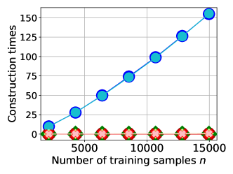
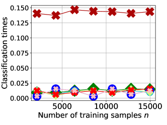
Figure 6: Construction and evaluation times for the algorithms studied in the Experimental study section.

We consider the methods listed in Figure 2 (top). The dataset was split into training ($80\%$) and testing ($20\%$) sets. In Figure 2 (top) we show the error obtained on the test set, over 5 realizations of the random splitting. The compression ratios achieved are shown on the bottom. The runtime for construction and evaluation are given in Figure 6 in the supplementary material. The parameters $\gamma=0.11$ for OptiNet and $k=10$ for $k$-NN were chosen by a validation procedure. The same $k$ is used for Proto-$k$-NN, while its compression sizes $m_{n}$ were matched to that of OptiNet.

The results highlight the following: (i) $k$-NN achieves the smallest error, but does not compress the data. $1$-NN’s error lags behind and further compressing its prototype set (the latter being the whole training dataset) using ProtoComp gives non-trivial compression rates without changing the error; (ii) OptiNet and Proto-$k$-NN achieves slightly better error than $1$-NN, but not as good as $k$-NN. Further compressing OptiNet and Proto-$k$-NN using ProtoComp gives highly compressed prototype sets without changing the errors, with an advantage to Proto-$k$-NN. The final prototype set of ProtoComp as applied on Proto-$k$-NN is shown in the bottom of Figure 1.

Conclusion

In this paper we study jointly-achievable error and compression rates for OptiNet in a common non-parametric classification setting. We believe our techniques can be extended to derive such rates for Proto-NN, Proto-$k$-NN, and the more advanced adaptive rules mentioned in the Introduction, as well as for the fast hierarchical compression heuristic proposed by Gottlieb, Kontorovich, and Nisnevitch (2014). The latter is particularly important, since the computational feasibility of the prototype rules studied here rapidly deteriorates as the dimension of the instance space increases. Studying compression rates in terms of the average margin of Ashlagi, Gottlieb, and Kontorovich (2021), and extending the results to metric losses (Cohen and Kontorovich 2022), are also compelling.

More fundamentally, given the universal consistency of OptiNet and Proto-NN in any separable metric space, the extension of our results beyond the Euclidean space is of interest. In particular, Theorem 2 shows that in $({\mathbb{R}}^{d},{\lVert\cdot\rVert}_{2})$ one can remove all spurious prototypes simultaneously, essentially without altering the classifier. We conjecture that this holds also for the $\ell_{p}$-norm for any $p\in(1,\infty)$. However, in more general metric spaces, Theorem 2 can fail, in the sense that removing all spurious prototypes simultaneously might lead to a classifier that is not consistent with the original one; see the supplementary material for a concrete example. In that case, one can use the iterative version of the compression (see the Further Compression section) while computing the neighboring cells using the heuristic ProtoCompApprox in (14). However, the theoretical properties of this lossy compression scheme are currently unknown. We leave these and related problems to future research.

Supplementary Material

Table 1 summarizes the error and compression rates available for various prototype learning rules. Table 2 summarizes the notation used throughout the paper. In Figure 6 we show the construction and evaluation runtimes for the algorithms studied in the Experimental study section. Procedure 1 is a pseudocode for ProtoComp and ProtoCompApprox. In this part we also provide proofs for the theorems that are provided in the paper and discuss Theorem 2.

Proofs

Additional notation we use are

$${\bar{B}}_{r}(x):=\{x^{\prime}\in{\cal X}:\rho(x,x^{\prime})\leq r\}$$

to denote the closed sphere around a given point $x\in{\cal X}$ with a given radius $r\geq 0$, and

$$\text{Seg}(x,x^{\prime}):=\{(1-u)x+ux^{\prime}:0\leq u\leq 1\}$$

to denote the segment between two given points $x,x^{\prime}\in{\cal X}$. For any $n\in\mathbb{N}$ we let $[n]:=\{1,2,\dots,n\}$.

Proof of Theorem 1

For any measurable decision function $g:{\cal X}\to\mathcal{Y}$,

$${\mathbb{P}}\{g(X)\neq Y\mid X\} =1-{\mathbb{P}}\{g(X)=Y\mid X\}$$

$$=1-\sum_{j=1}^{M}{\mathbb{P}}\{g(X)=Y=j\mid X\}$$

$$=1-\sum_{j=1}^{M}\mathbb{I}_{\{g(X)=j\}}P_{j}(X)$$

$$=1-P_{g(X)}(X).$$

This implies

$${\mathbb{E}}\{L(g_{n})\}-L^{*} ={\mathbb{E}}\{P_{g^{*}(X)}(X)-P_{g_{n}(X)}(X)\}$$

$$={\mathbb{E}}\left\{\int(P_{g^{*}(x)}(x)-P_{g_{n}(x)}(x))\mu(dx)\right\}$$

$$\leq{\mathbb{E}}\left\{L_{\gamma}\right\}+{\mathbb{E}}\left\{\int_{{\rm UB(\gamma)}}(P_{g^{*}(x)}(x)-P_{g_{n}(x)}(x))\mu(dx)\right\},$$ (18)

where ${\rm UB(\gamma)}$ is the $\gamma$-envelope around ${{\bf X}^{\prime}_{m}}$,

$${\rm UB(\gamma)}=\bigcup_{i=1}^{m}B_{\gamma}(X^{\prime}_{i}),$$ (19)

where $B_{\gamma}(x)=\{x^{\prime}\in{\cal X}:\rho(x,x^{\prime})<\gamma\}$ is the open ball around $x$ with radius $\gamma$, and

$$L_{\gamma}:=L_{\gamma}({{\bf X}^{\prime}_{m}}):=\mu({\cal X}\setminus{\rm UB(\gamma)})$$

is the $\gamma$-missing-mass of ${{\bf X}^{\prime}_{m}}$, and $g_{n}:=g_{n,m,\gamma}$. By the law of total expectation,

$${\mathbb{E}}\left\{\int_{{\rm UB(\gamma)}}(P_{g^{*}(x)}(x)-P_{g_{n}(x)}(x))\mu(dx)\right\}$$

$$={\mathbb{E}}\left\{\int_{{\rm UB(\gamma)}}{\mathbb{E}}\left\{(P_{g^{*}(x)}(x)-P_{g_{n}(x)}(x))\mathbb{I}_{\{g^{*}(x)\neq g_{n}(x)\}}\mu(dx)\mid{{\bf X}^{\prime}_{m}}\right\}\right\}$$

$$={\mathbb{E}}\left\{\int_{{\rm UB(\gamma)}}{\mathbb{E}}\{I_{n}(x)\mid{{\bf X}^{\prime}_{m}}\}\mu(dx)\right\},$$

where

$$I_{n}(x) =(P_{g^{*}(x)}(x)-P_{g_{n}(x)}(x))\mathbb{I}_{\{P_{g^{*}(x)}(x)>P_{g_{n}(x)}(x)\}}\mathbb{I}_{\{P_{n,g_{n}(x)}(x)\geq P_{n,g^{*}(x)}(x)\}}.$$

For all $x\in{\cal X}$ abbreviate $V_{x}:=V_{x}({{\bf X}}(\gamma))$ as the Voronoi cell containing $x$ and let

$$P_{n,j}(x):=\frac{\frac{1}{n}\sum_{X_{i}\in{{\bf X}_{n}}}\mathbb{I}_{\{Y_{i}=j,X_{i}\in V_{x}\}}}{\mu(V_{x})}.$$

(Note that in the main text, $P_{n,\ell,j}$ is defined differently for convenience, but one can easily verify that it corresponds to the same classifier.) The relation

$$\{P_{n,g_{n}(x)}(x)-P_{n,g^{*}(x)}(x)\geq 0\}$$

$$=\{P_{n,g_{n}(x)}(x)-P_{g_{n}(x)}(x)+P_{g_{n}(x)}(x)-P_{g^{*}(x)}(x)+P_{g^{*}(x)}(x)-P_{n,g^{*}(x)}(x)\geq 0\}$$

$$\subseteq\left\{\sum_{j=1}^{M}|P_{n,j}(x)-P_{j}(x)|\geq P_{g^{*}(x)}(x)-P_{g_{n}(x)}(x)\right\}$$

yields

$$\quad\,\,\mathbb{I}_{\{P_{g^{*}(x)}(x)>P_{g_{n}(x)}(x)\}}\mathbb{I}_{\{P_{n,g_{n}(x)}(x)\geq P_{n,g^{*}(x)}(x)\}}$$

$$\leq\mathbb{I}_{\{\sum_{j=1}^{M}|P_{n,j}(x)-P_{j}(x)|\geq P_{g^{*}(x)}(x)-P_{g_{n}(x)}(x)\}}.$$

Thus,

$$I_{n}(x)$$

$$\leq\sum_{\ell=1}^{M}(P_{g^{*}(x)}(x)-P_{\ell}(x))\mathbb{I}_{\{\sum_{j=1}^{M}|P_{n,j}(x)-P_{j}(x)|\geq P_{g^{*}(x)}(x)-P_{\ell}(x)\}}\mathbb{I}_{\{g_{n}(x)=\ell\neq g^{*}(x)\}}$$

$$\leq\sum_{\ell=1}^{M}(P_{g^{*}(x)}(x)-P_{\ell}(x))\mathbb{I}_{\{\sum_{j=1}^{M}|P_{n,j}(x)-P_{j}(x)|\geq P_{g^{*}(x)}(x)-P_{\ell}(x)\}}\mathbb{I}_{\{\ell\neq g^{*}(x)\}}$$

$$\leq\sum_{j=1}^{M}\sum_{\ell=1}^{M}(P_{g^{*}(x)}(x)-P_{\ell}(x))\mathbb{I}_{\{\ell\neq g^{*}(x)\}}\mathbb{I}_{\{|P_{n,j}(x)-P_{j}(x)|\geq(P_{g^{*}(x)}(x)-P_{\ell}(x))/M\}}.$$

Given ${{\bf X}^{\prime}_{m}}$, for every $j\in\mathcal{Y}$ put

$$\bar{P}_{n,j}(x) :=\frac{\frac{1}{n}{\mathbb{E}}\{\sum_{X_{i}\in{\bf X}_{n}}\mathbb{I}_{\{Y_{i}=j,X_{i}\in V_{x}\}}\mid{{\bf X}^{\prime}_{m}}\}}{\mu(V_{x})}$$

$$=\frac{\int_{V_{x}}P_{j}(z)\mu(dz)}{\mu(V_{x})}.$$ (20)

Noting that

$$|P_{j}(x)-P_{n,j}(x)| \leq|P_{j}(x)-\bar{P}_{n,j}(x)|+|\bar{P}_{n,j}(x)-P_{n,j}(x)|$$

and denoting

$$D_{\ell}^{*}(x):=(P_{g^{*}(x)}(x)-P_{\ell}(x))\mathbb{I}_{\{\ell\neq g^{*}(x)\}},$$

we have that

$$I_{n}(x) \leq\sum_{j,\ell=1}^{M}D_{\ell}^{*}(x)\mathbb{I}_{\{|P_{n,j}(x)-P_{j}(x)|\geq D_{\ell}^{*}(x)/M\}}$$

$$\leq\sum_{j,\ell=1}^{M}D_{\ell}^{*}(x)\mathbb{I}_{\{|P_{n,j}(x)-\bar{P}_{n,j}(x)|\geq D_{\ell}^{*}(x)/2M\}}$$

$$\quad+\sum_{j,\ell=1}^{M}D_{\ell}^{*}(x)\mathbb{I}_{\{|\bar{P}_{n,j}(x)-P_{j}(x)|\geq D_{\ell}^{*}(x)/2M\}}.$$

Thus,

$$\int_{{\rm UB(\gamma)}}{\mathbb{E}}\{I_{n}(x)\mid{{\bf X}^{\prime}_{m}}\}\mu(dx) \leq\sum_{j,\ell=1}^{M}J_{n,1,j,\ell}+\sum_{j,\ell=1}^{M}J_{n,2,j,\ell},$$

where

$$J_{n,1,j,\ell} :=\int_{{\rm UB(\gamma)}}D_{\ell}^{*}(x){\mathbb{P}}\{|P_{n,j}(x)-\bar{P}_{n,j}(x)|\geq D_{\ell}^{*}(x)/2M\mid{{\bf X}^{\prime}_{m}}\}\mu(dx)$$ (21)

and

$$J_{n,2,j,\ell} :=\int_{{\rm UB(\gamma)}}D_{\ell}^{*}(x)\mathbb{I}_{\{|\bar{P}_{n,j}(x)-P_{j}(x)|\geq D_{\ell}^{*}(x)/2M\}}\mu(dx).$$

Concerning the estimation error (21), $J_{n,1,j,\ell}$, for all $j\in[M]$, $i\in[n]$, and $x\in{\cal X}$, we define the random variables

$$K_{n,i,j}(x)=\mathbb{I}_{\{Y_{i}=j,X_{i}\in V_{x}\}}.$$

Given ${{\bf X}^{\prime}_{m}}$, for all $j\in\mathcal{Y}$, $(K_{n,i,j})_{i=1}^{n}$ are i.i.d. Hence, the Bernstein inequality yields

$${\mathbb{P}}\left\{\left|P_{n,j}(x)-\bar{P}_{n,j}(x)\right|\geq D_{\ell}^{*}(x)/2M\mid{{\bf X}^{\prime}_{m}}\right\}$$

$$={\mathbb{P}}\left\{\left|\frac{1}{n}\sum_{i=1}^{n}\left(K_{n,i,j}(x)-{\mathbb{E}}\left\{K_{n,i,j}(x)\mid{{\bf X}^{\prime}_{m}}\right\}\right)\right|\geq\mu(V_{x})D_{\ell}^{*}(x)/2M\mid{{\bf X}^{\prime}_{m}}\right\}$$

$$\leq 2\exp\left(-\frac{n}{2}\frac{(\mu(V_{x})D_{\ell}^{*}(x))^{2}}{4M^{2}}\frac{1}{\mathbb{V}\{K_{n,1,j}(x)\mid{{\bf X}^{\prime}_{m}}\}+\frac{\mu(V_{x})D_{\ell}^{*}(x)}{3\cdot 2M}}\right)$$

$$=:\left(*\right).$$

Considering the variance

$$\mathbb{V}\!\left\{K_{n,1,j}(x)\mid{{\bf X}^{\prime}_{m}}\right\}$$

$$={\mathbb{P}}\left\{Y_{1}=j,X_{1}\in V_{x}\mid{{\bf X}^{\prime}_{m}}\right\}\cdot\left(1-{\mathbb{P}}\{Y_{1}=j,X_{1}\in V_{x}\mid{{\bf X}^{\prime}_{m}}\}\right)$$

$$\leq{\mathbb{P}}\left\{Y_{1}=j,X_{1}\in V_{x}\mid{{\bf X}^{\prime}_{m}}\right\}$$

$$\leq{\mathbb{P}}\left\{X_{1}\in V_{x}\mid{{\bf X}^{\prime}_{m}}\right\}$$

$$=\mu(V_{x}).$$

In addition, $D_{\ell}^{*}(x)\leq 1$. Consequently,

$$\left(*\right) \leq 2\exp\left(-\frac{n(\mu(V_{x})D_{\ell}^{*}(x))^{2}}{8M^{2}}\cdot\frac{1}{\mu(V_{x})+\frac{\mu(V_{x})}{6M}}\right)$$

$$\leq 2\exp\left(-\frac{3n\mu(V_{x})D_{\ell}^{*}(x)^{2}}{28M^{2}}\right).$$

Towards applying the margin condition, we first lower bound $\mu(V_{x})$. By the packing and covering properties of $\gamma$-nets, for any nucleus $q\in{{\bf X}}(\gamma)$,

$$B_{\gamma/2}(q)\subseteq V_{q}.$$ (22)

Indeed, if some $x$ has $\rho(q,x)<\gamma/2$ but $x\notin V_{q}$, then $x$ belongs to a Voronoi cell whose nucleus $q^{\prime}\neq q$ is such that

$$\rho(x,q^{\prime})\leq\rho(x,q)<\gamma/2.$$

This however implies

$$\rho(q,q^{\prime})\leq\rho(q,x)+\rho(x,q^{\prime})<\gamma/2+\gamma/2=\gamma,$$

in contradiction to the requirement that $q$ and $q^{\prime}$ must have interdistance larger or equal to $\gamma$.

Denote by $q_{x}$ the nucleus in ${{\bf X}^{\prime}_{m}}$ corresponding to $V_{x}$. Using (22), the MMC in (3) and the BAZ assumption in (4), we have that for $\gamma\leq 2\gamma_{0}$,

$$\mu(V_{x})\geq\mu(B_{\gamma/2}(q_{x}))\geq\kappa\nu_{0}(\gamma/2)^{d}.$$

Thus, assuming $\gamma\leq 2\gamma_{0}$,

$${\mathbb{P}}\left\{\left|P_{n,j}(x)-\bar{P}_{n,j}(x)\right|\geq D_{\ell}^{*}(x)/2M\mid{{\bf X}^{\prime}_{m}}\right\} \leq 2\exp\left(-\frac{3\kappa\nu_{0}\cdot n\gamma^{d}D_{\ell}^{*}(x)^{2}}{28\cdot 2^{d}M^{2}}\right)$$

$$=2\exp\left(-c_{d}n\gamma^{d}D_{\ell}^{*}(x)^{2}\right).$$

Therefore,

$$J_{n,1,j,l} \leq 2\int_{{\rm UB(\gamma)}}D_{\ell}^{*}(x)\exp\left(-c_{d}n\gamma^{d}D_{\ell}^{*}(x)^{2}\right)\mu(dx)$$

$$\leq 2\int D_{\ell}^{*}(x)\exp\left(-c_{d}n\gamma^{d}D_{\ell}^{*}(x)^{2}\right)\mu(dx).$$

The margin condition with parameter $\alpha$ means that for $0\leq t\leq 1$,

$$G(t) :={\mathbb{P}}\left\{D_{\ell}^{*}(X)\leq t\right\}\leq{\mathbb{P}}\left\{P_{(1)}(X)-P_{(2)}(X)\leq t\right\}\leq c^{*}\cdot t^{\alpha}.$$

Thus, applying integration by parts as in (Döring, Györfi, and Walk 2017, Lemma 2),

$$J_{n,1,j,l} \leq 2\int_{0}^{1}s\exp\left(-c_{d}n\gamma^{d}s^{2}\right)G(ds)$$

$$=2e^{-c_{d}n\gamma^{d}}-2\int_{0}^{1}\exp\left(-c_{d}n\gamma^{d}s^{2}\right)\left(1-2c_{d}n\gamma^{d}s^{2}\right)G(s)\,ds$$

$$\leq 2e^{-c_{d}n\gamma^{d}}+2c^{*}c_{d}n\gamma^{d}\int_{0}^{1}\exp\left(-c_{d}n\gamma^{d}s^{2}\right)s^{2+\alpha}\,ds$$

$$\leq 2e^{-c_{d}n\gamma^{d}}+2c^{*}(c_{d}n\gamma^{d})^{-(1+\alpha)/2}\int_{0}^{\infty}\exp\left(-u^{2}/8\right)u^{2+\alpha}\,du$$

$$=O\left(\left(n\gamma^{d}\right)^{-(\alpha+1)/2}\right).$$

To bound the approximation error (23), the Hölder continuity assumption implies that for all $x\in{\rm UB(\gamma)}$,

$$\left|\bar{P}_{n,j}(x)-P_{j}(x)\right|$$

$$=\left|\frac{1}{\mu(V_{x})}\int_{V_{x}}P_{j}(z)\mu(dz)-\frac{1}{\mu(V_{x})}\int_{V_{x}}P_{j}(x)\mu(dz)\right|$$

$$\leq\frac{1}{\mu(V_{x})}\int_{V_{x}}\left|P_{j}(z)-P_{j}(x)\right|\mu(dz)$$

$$=\frac{1}{\mu(V_{x})}\int_{V_{x}\setminus{\rm UB(\gamma)}}\left|P_{j}(z)-P_{j}(x)\right|\mu(dz)+\frac{1}{\mu(V_{x})}\int_{V_{x}\cap{\rm UB(\gamma)}}\left|P_{j}(z)-P_{j}(x)\right|\mu(dz)$$

$$\leq\frac{\mu(V_{x}\setminus{\rm UB(\gamma)})}{\mu(V_{x})}+\frac{1}{\mu(V_{x})}\int_{V_{x}\cap{\rm UB(\gamma)}}C\rho(x,z)^{\beta}\mu(dz).$$

For the second term, since both $x$ and $z$ belong to $V_{x}\cap{\rm UB(\gamma)}$ they both share the same prototype in ${{\bf X}}(\gamma)$, and since ${{\bf X}}(\gamma)$ is a $\gamma$-net of ${{\bf X}^{\prime}_{m}}$ it holds that $X^{(1)}(x;{{\bf X}}(\gamma))\leq 2\gamma$ and $X^{(1)}(z;{{\bf X}}(\gamma))\leq 2\gamma$. Thus, for $x\in{\rm UB(\gamma)}$,

$$\rho(x,z)\leq X^{(1)}(x;{{\bf X}}(\gamma))+X^{(1)}(z;{{\bf X}}(\gamma))\leq 2\gamma+2\gamma=4\gamma.$$

Hence, for $x\in{\rm UB(\gamma)}$,

$$\left|\bar{P}_{n,j}(x)-P_{j}(x)\right|\leq\frac{\mu(V_{x}\setminus{\rm UB(\gamma)})}{\mu(V_{x})}+C(4\gamma)^{\beta}.$$

Hence,

$$J_{n,2,j,\ell} =\int_{{\rm UB(\gamma)}}D_{\ell}^{*}(x)\mathbb{I}_{\{|\bar{P}_{n,j}(x)-P_{j}(x)|\geq D_{\ell}^{*}(x)/2M\}}\mu(dx)$$

$$\leq\int_{{\rm UB(\gamma)}}D_{\ell}^{*}(x)\mathbb{I}_{\{\frac{\mu(V_{x}\setminus{\rm UB(\gamma)})}{\mu(V_{x})}+C(4\gamma)^{\beta}\geq D_{\ell}^{*}(x)/2M\}}\mu(dx)$$

$$\leq\int_{{\rm UB(\gamma)}}D_{\ell}^{*}(x)\mathbb{I}_{\{4M\frac{\mu(V_{x}\setminus{\rm UB(\gamma)})}{\mu(V_{x})}\geq D_{\ell}^{*}(x)\}}\mu(dx)+\int_{{\rm UB(\gamma)}}D_{\ell}^{*}(x)\mathbb{I}_{\{4MC(4\gamma)^{\beta}\geq D_{\ell}^{*}(x)\}}\mu(dx)$$

$$\leq 4M\mu({\cal X}\setminus{\rm UB(\gamma)})+\int D_{\ell}^{*}(x)\mathbb{I}_{\{2CM(4\gamma)^{\beta}\geq D_{\ell}^{*}(x)\}}\mu(dx).$$ (23)

For the second term in (23), the margin condition yields

$$\int D_{\ell}^{*}(x)\mathbb{I}_{\{2CM(4\gamma)^{\beta}\geq D_{\ell}^{*}(x)\}}\mu(dx) =\int s\cdot\mathbb{I}_{\{s\leq 2CM(4\gamma)^{\beta}\}}G(ds)$$

$$\leq 2CM(4\gamma)^{\beta}\int_{0}^{2CM(4\gamma)^{\beta}}G(ds)$$

$$\leq c^{*}\alpha\left(2CM(4\gamma)^{\beta}\right)^{\alpha+1}$$

$$=O(\gamma^{\beta(\alpha+1)}).$$

The first term in (23) is proportional to $L_{\gamma}$, as the term in (18), whose expectation is bounded by

$${\mathbb{E}}\{L_{\gamma}\} ={\mathbb{E}}\left\{\int\mathbb{I}_{\{x\notin{\rm UB(\gamma)}\}}\mu(dx)\right\}$$

$$=\int{\mathbb{E}}\left\{\mathbb{I}_{\{x\notin{\rm UB(\gamma)}\}}\right\}\mu(dx)$$

$$=\int{\mathbb{P}}\left\{\rho(x,X^{(1)}(x;{\bf X}^{\prime}_{m}))\geq\gamma\right\}\mu(dx)$$

$$=\int\left(1-\mu(B_{\gamma}(x))\right)^{m}\mu(dx)$$

$$\leq\int\exp\left(-m\mu(B_{\gamma}(x))\right)\mu(dx).$$

Applying the MMC in (3), followed by the BAZ assumption (4), we have that for $x\in\mathcal{S}(\mu)$,

$$\exp\left(-m\mu(B_{\gamma}(x))\right)\leq\exp\left(-\kappa m\gamma^{d}f(x)\right)\leq\exp\left(-\kappa m\gamma^{d}\nu_{0}\right).$$

Hence,

$${\mathbb{E}}\{L_{\gamma}\} \leq\exp\left(-\kappa\nu_{0}m\gamma^{d}\right)=\exp\left(-\Omega(m\gamma^{d})\right),$$

concluding the proof. ∎

Proof of Theorem 2

Under the event that all the instance-label pairs have the same label, (13) trivially holds and we are done. Henceforth, we assume the complementary. Since $\mu$ has a density, the event

$$\{X^{\prime}_{i}\neq X^{\prime}_{j},\quad\text{for any distinct $i,j\in[m]$}\}$$ (24)

occurs with probability one, and so, we assume the event in (24) as well. Denote $(\widetilde{\bf X},\widetilde{\bf Y})=\widetilde{\cal D}$. As reasoned by the following lemma whose proof is given below, we also assume that $\widetilde{\cal D}\neq\emptyset$. This implies that $X^{(1)}(x;\widetilde{\bf X})$ exists for any $x\in{\cal X}$.

Lemma 4.

Under the notation and assumptions of Theorem 2, the event $\{\widetilde{\cal D}\neq\emptyset\}$ occurs with probability one.

As will become clear below, the following lemma shows that the set on which (13) fails has zero Lebesgue measure.

Lemma 5.

Assume that $\rho$ is the Euclidean metric. Let ${\bf X}^{\prime}=\{X^{\prime}_{1},\dots,X^{\prime}_{m}\}\subseteq{\cal X}={\mathbb{R}}^{d}$ be a set of $m$ distinct examples. For all $i,j,l\in[m]$, let

$$F_{i,j,l}:=\{x^{\prime}\in{\cal X}:\rho(x^{\prime},X^{\prime}_{i})=\rho(x^{\prime},X^{\prime}_{j})=\rho(x^{\prime},X^{\prime}_{l})\}$$ (25)

and

$$\widehat{F}_{i,j,l}:=\{x^{\prime}\in{\cal X}:x^{\prime}\text{ is a linear combination of elements from }F_{i,j,l}\cup\{X^{\prime}_{i}\}\},$$ (26)

and define

$$\widehat{F}:=\bigcup_{\begin{subarray}{c}\text{distinct}\\ i,j,l\in[m]\end{subarray}}\widehat{F}_{i,j,l}.$$ (27)

Then,

$$\lambda(\widehat{F})=0.$$

Let $\widehat{F}$ be as in (27). By the assumption that each nucleus in ${\bf X}^{\prime}$ is unique (that is, the assumption on the event in (24)), and by Lemma 5, it suffices to show that (13) holds for all $x\in{\cal X}\setminus\widehat{F}$. So, fix $x\in{\cal X}\setminus\widehat{F}$.

Lemma 6.

Let $x\in{\cal X}\setminus\widehat{F}$, where $\widehat{F}$ is as in (27). Under the assumptions of Theorem 2, assume that $|{\cal D}^{\prime}|=m$. For all $k\in[m]$, denote

$$q_{k}:=X^{(k)}(x;{\bf X}^{\prime}).$$ (28)

If the event in (24) occurs, then

$$\forall\,2\leq i\leq m,\ \exists\,1\leq j<i\qquad\text{s.t.}\qquad q_{i}\in\mathcal{N}(q_{j},{\bf X}^{\prime}).$$ (29)

The remaining of the proof is demonstrated in Figure 3.

Figure 3: A demonstration of the induction in the proof of Theorem 2 for a private example. Assume that $\widetilde{\cal D}=\{q_{4},q_{5}\}$. Since $q_{4}$ is the nearest neighbour of $x$ from among $\widetilde{\bf X}$, then, $q_{i_{1}}=q_{4}$. An index $j\in[4-1]$ that is guaranteed by Lemma 6 to satisfy $q_{j}\in\mathcal{N}(q_{4},{\cal D}^{\prime})$ is, for example, $j=3$. So, $q_{i_{2}}=q_{3}$. Since $q_{3}\notin\widetilde{\bf X}$, then, by the definition of $\widetilde{\cal D}$ in (12), $Y^{\prime}(q_{3})=Y^{\prime}(q_{4})$. Repeating this argument, by Lemma 6, an index $j\in[3-1]$ such that $q_{j}\in\mathcal{N}(q_{3},{\cal D}^{\prime})$ is, for example, $j=1$. So, $q_{i_{3}}=q_{1}$. Since $q_{1}\notin\widetilde{\bf X}$, then, $Y^{\prime}(q_{1})=Y^{\prime}(q_{3})$. Finally, $Y^{\prime}(q_{4})$, the label of $x$ according to $\widetilde{\cal D}$, is equal to $Y^{\prime}(q_{1})$, the label of $x$ according to ${\cal D}^{\prime}$, and so, $Y^{(1)}(x;\widetilde{\cal D})=Y^{(1)}(x;{\cal D}^{\prime})$.

Let $i_{1}\in[m]$ be the index for which $q_{i_{1}}=X^{(1)}(x;\widetilde{\bf X})$. Proving by induction, suppose that we have already established a sequence $m\geq i_{1}>i_{2}>\dots>i_{l}\geq 1$ for some $1\leq l\leq m$ such that $q_{i_{j}}\in\mathcal{N}(q_{i_{j+1}},{\bf X}^{\prime})$ and $Y^{\prime}(q_{i_{j+1}})=Y^{\prime}(q_{i_{1}})$ for all $j=1,\dots,l-1$. If $i_{l}>1$, then, by Lemma 6, there exists $1\leq i_{l+1}<i_{l}$ such that $q_{i_{l}}\in\mathcal{N}(q_{i_{l+1}},{\bf X}^{\prime})$. Recall that by the definition in (28), $q_{k}=X^{(k)}(x;{\bf X}^{\prime})$ for all $k\in[m]$. So, by $i_{l+1}<i_{l}\leq i_{1}$, $q_{i_{l+1}}$ is closer to $x$ than $q_{i_{1}}$. Thus, we must have that ${q_{i_{l+1}}}\notin\widetilde{\bf X}$ (because otherwise $q_{i_{1}}$ wouldn’t have been equal to $X^{(1)}(x;\widetilde{\bf X})$). In turn, by the definition of $\widetilde{\cal D}$ in (12) and by $q_{i_{l}}\in\mathcal{N}(q_{i_{l+1}},{\bf X}^{\prime})$, this implies that $Y^{\prime}(q_{i_{l+1}})=Y^{\prime}(q_{i_{l}})$. By the induction’s assumption $Y^{\prime}(q_{i_{l}})=Y^{\prime}(q_{i_{1}})$. So, $Y^{\prime}(q_{i_{l+1}})=Y^{\prime}(q_{i_{1}})$. Repeating the inductive step no more than $m-1$ iterations, this process must eventually produce the index $i_{l^{\prime}}=1$ for some $l^{\prime}\in[m]$, per (29). So, as guaranteed,

$$Y^{(1)}(x;\widetilde{\cal D})=Y^{\prime}(q_{i_{1}})=Y^{\prime}(q_{i_{l^{\prime}}})=Y^{\prime}(q_{1})=Y^{(1)}(x;{\cal D}^{\prime}).$$

This concludes the proof. ∎

Proof of Lemma 4

Under the event that all the instance-label pairs have the same label, $\widetilde{\cal D}\neq\emptyset$ by its definition in Theorem 2. So, assume the complementary. If ${\cal D}^{\prime}$ contains $m\in\mathbb{N}$ instance-label pairs, assume also the event where $X^{\prime}_{i^{\prime}}\neq X^{\prime}_{j^{\prime}}$ for any distinct $i^{\prime},j^{\prime}\in[m]$. Since $\mu$ has a density, this event occurs with probability one.

Let

$$\{i,j\}:=\mathop{\rm arg\,min}_{\{i^{\prime},j^{\prime}\}\subseteq[m]:\ Y^{\prime}(X^{\prime}_{i^{\prime}})\neq Y^{\prime}(X^{\prime}_{j^{\prime}})}\rho(X^{\prime}_{i^{\prime}},X^{\prime}_{j^{\prime}})$$ (30)

and

$$p_{0}:=(X^{\prime}_{i}+X^{\prime}_{j})/2.$$ (31)

By $Y^{\prime}(X^{\prime}_{i})\neq Y^{\prime}(X^{\prime}_{j})$, $X^{\prime}_{i}\neq X^{\prime}_{j}$. Directly from the definition of $\mathcal{N}$ in (11), $X^{(2)}(p_{0};{\bf X}^{\prime})\in\mathcal{N}(X^{(1)}(p_{0};{\bf X}^{\prime}),{\bf X}^{\prime})$. We will show that

$$\{X^{(1)}(p_{0};{\bf X}^{\prime}),X^{(2)}(p_{0};{\bf X}^{\prime})\}=\{X^{\prime}_{i},X^{\prime}_{j}\}.$$ (32)

Then, letting $(\widetilde{\bf X},\widetilde{\bf Y})=\widetilde{\cal D}$, by the definition of $\widetilde{\cal D}$ in (12) and by $Y^{\prime}(X^{\prime}_{i})\neq Y^{\prime}(X^{\prime}_{j})$, we will have that $X^{(1)}(p_{0};{\bf X}^{\prime})\in\widetilde{\bf X}$. This will imply $\widetilde{\cal D}\neq\emptyset$.

So, towards (32), let $r_{0}:=\rho(p_{0},X^{\prime}_{i})=\rho(p_{0},X^{\prime}_{j})$, and suppose in a contradiction that there exists $l\in[m]\setminus\{i,j\}$ such that

$$X^{\prime}_{l}\in{\bar{B}}_{r_{0}}(p_{0}).$$

Since $Y(X^{\prime}_{i})\neq Y^{\prime}(X^{\prime}_{j})$, then $Y^{\prime}(X^{\prime}_{l})\neq Y^{\prime}(X^{\prime}_{i})$ or $Y^{\prime}(X^{\prime}_{l})\neq Y^{\prime}(X^{\prime}_{j})$. W.L.O.G. assume the former. By our assumption, $j\neq l$ implies

$$X^{\prime}_{j}\neq X^{\prime}_{l}.$$

By the definition of $p_{0}$ in (31), $X^{\prime}_{i}$ and $X^{\prime}_{j}$ are antipodal points of ${\bar{B}}_{r_{0}}(p_{0})$. Thus, from the geometrical properties of ${\mathbb{R}}^{d}$, the fact that $\rho$ is the Euclidean metric and $X^{\prime}_{l}\in{\bar{B}}_{r_{0}}(p_{0})\setminus\{X^{\prime}_{j}\}$, we have that $\rho(X^{\prime}_{i},X^{\prime}_{l})<\rho(X_{i}^{\prime},X^{\prime}_{j})$. This is a contradiction to the definition of $i$ and $j$ in (30). Hence, every nucleus $X^{\prime}_{l}$, $l\in[m]\setminus\{i,j\}$, is strictly farther from $p_{0}$ than $X^{\prime}_{i}$ and $X^{\prime}_{j}$. This implies (32). ∎

Proof of Lemma 5

We say that $F\subseteq{\mathbb{R}}^{d}$ is a $k$-flat if it is a $k$-dimensional affine subspace of $\mathbb{R}^{d}$, $1\leq k\leq d$. A $0$-flat is a singleton in $\mathbb{R}^{d}$ and a $(-1)$-flat is the empty set. A $(d-1)$-flat is called a hyperplane. For all $i,j\in[m]$ define

$$F_{i,j}:=\{x\in{\cal X}:\rho(x,X^{\prime}_{i})=\rho(x,X^{\prime}_{j})\},$$

and note that given also $l\in[m]$, $F_{i,j,l}=F_{i,j}\cap F_{i,l}$.

Let distinct $i,j,l\in[m]$. Using $X^{\prime}_{j}\neq X^{\prime}_{i}\neq X^{\prime}_{l}$ and the fact that $\rho$ is the Euclidean metric, one can easily show that $F_{i,j}$ and $F_{i,l}$ are hyperplanes. Suppose in a contradiction that $F_{i,j}=F_{i,l}$. Let $x_{j}:=(X^{\prime}_{i}+X^{\prime}_{j})/2$ and $x_{l}:=(X^{\prime}_{i}+X^{\prime}_{l})/2$. Since $\rho$ is the Euclidean metric, $x_{j}\in F_{i,j}$ and $x_{l}\in F_{i,l}$. By $F_{i,j}=F_{i,l}$, $x_{j},x_{l}\in F_{i,j,l}$. Now, let $r_{j}:=\rho(x_{j},X^{\prime}_{i})$ and $r_{l}:=\rho(x_{l},X^{\prime}_{i})$.

By $x_{j}\in F_{i,j,l}$, $\rho(x_{j},X^{\prime}_{l})=r_{j}$. So, $X_{l}^{\prime}\in{\bar{B}}_{r_{j}}(x_{j})\setminus\{X^{\prime}_{j}\}$. In addition, note that $X^{\prime}_{i}$ and $X^{\prime}_{j}$ are antipodal points in the close sphere ${\bar{B}}_{r_{j}}(x_{j})$. By these two observations, by the geometry of ${\mathbb{R}}^{d}$ and due to the fact that $\rho$ is the Euclidean metric, we must have that $\rho(X^{\prime}_{i},X^{\prime}_{l})<\rho(X^{\prime}_{i},X^{\prime}_{j})$. On the other hand, exchanging the roles of the indices $j$ and $l$ in this paragraph yields $\rho(X^{\prime}_{i},X^{\prime}_{j})<\rho(X^{\prime}_{i},X^{\prime}_{l})$. This is a contradiction. Thus, $F_{i,j}\neq F_{i,l}$.

It can be shown that the intersection of two distinct hyperplanes is a $k$-flat for some $k\in\{d-2,-1\}$. So, $F_{i,j,l}=F_{i,j}\cap F_{i,l}$ is a $k_{i,j,l}$-flat for a certain $k_{i,j,l}\in\{d-2,-1\}$. Since $F_{i,j,l}$ is a $k_{i,j,l}$-flat and $X^{\prime}_{i}\notin F_{i,j,l}$, one can verify that that $\widehat{F}_{i,j,l}$ is a $(k_{i,j,l}+1)$-flat. Using elementary tools of measure theory, it can be proved that the Lebesgue measure of any $k^{\prime}$-flat is zero, for all $k^{\prime}<d$. Thus, $\lambda(\widehat{F}_{i,j,l})=0$. By the generality of the $i,j$ and $l$,

$$\lambda(\widehat{F})\leq\sum_{\begin{subarray}{c}\text{distinct}\\ i,j,l\in[m]\end{subarray}}\lambda(\widehat{F}_{i,j,l})=0.$$

∎

Proof of Lemma 6

Fix some $2\leq i\leq m$. We will define a point $p_{2}$ and will show that its first- and second-NN’s are $q_{j}$ and $q_{i}$, respectively, for a certain $1\leq j<i$. By the definition of $\mathcal{N}$ in $\eqref{def:NNm}$, this will conclude the proof. A demonstration of the proof is shown in Figure 4.

For any $a,b,c,d\in{\cal X}$ define the following continuous function $\rho_{\text{Seg}(a,b)}^{c,d}:[0,1]\to{\mathbb{R}}$ () according to the rule

$$t\mapsto\rho((1-t)a+tb,c)-\rho((1-t)a+tb,d).$$

Since $i\neq 1$, (and by the assumption on the event in (24)), $q_{1}\neq q_{i}$. And so,

$$\rho_{\text{Seg}(q_{i},x)}^{q_{i},q_{1}}(0)=\rho(q_{i},q_{i})-\rho(q_{i},q_{1})<0.$$

By the definition of $q_{k},k\in[m]$, in (28),

$$\rho_{\text{Seg}(q_{i},x)}^{q_{i},q_{1}}(1)=\rho(x,q_{i})-\rho(x,q_{1})\geq 0.$$

By the Intermediate Value Theorem, the function $\rho_{\text{Seg}(q_{i},x)}^{q_{i},q_{1}}$ has a root $0<t^{\prime}\leq 1$. Then, $q_{1}$ and $q_{i}$ are equidistant to the point $x^{\prime}:=(1-t^{\prime})q_{i}+t^{\prime}x\in\text{Seg}(q_{i},x)\setminus\{q_{i}\}$. This, in turn, ensures us the existence of

$$p_{1}:=\mathop{\rm arg\,min}_{\begin{subarray}{c}p\in\text{Seg}(q_{i},x):\ \exists j<i,\rho(p,q_{j})=\rho(p,q_{i})\end{subarray}}\rho(p,q_{i})\in\text{Seg}(q_{i},x)\setminus\{q_{i}\}.$$ (33)

Define $r_{1}:=\rho(p_{1},q_{i})$, and fix an index $j\in[i-1]$ that satisfies $\rho(p_{1},q_{j})=r_{1}$. We will show that

$$\rho(p_{1},q_{l})>r_{1},\qquad\forall l\in[m]\setminus\{i,j\}.$$ (34)

For all $i^{\prime},j^{\prime},l^{\prime}\in[m]$, let $F_{i^{\prime},j^{\prime},l^{\prime}}$ and $\widehat{F}_{i^{\prime},j^{\prime},l^{\prime}}$ as are defined in (25) and in (26). Suppose in a contradiction that $\rho(p_{1},q_{l})=r_{1}$ for some $l\in[m]\setminus\{i,j\}$. For all $k\in[m]$, let $s_{k}\in[m]$ be the index for which $X^{\prime}_{s_{k}}=q_{k}$. So, $p_{1}\in F_{s_{i},s_{j},s_{l}}$. Since $p_{1}\in\text{Seg}(x,X^{\prime}_{s_{i}})$, $x$ is a linear combination of $p_{1}\in F_{s_{i},s_{j},s_{l}}$ with $X^{\prime}_{s_{i}}$. As such, by definition, $x\in\widehat{F}_{s_{i},s_{j},s_{l}}\subseteq\widehat{F}$. This is a contradiction to $x\notin\widehat{F}$.

Now, suppose in a contradiction that there exists $l\in[m]\setminus\{i,j\}$ s.t. $\rho(p_{1},q_{l})<r_{1}=\rho(p_{1},q_{i})$. In order to see that $l<i$, note that

$$\rho(x,q_{l}) \leq\rho(x,p_{1})+\rho(p_{1},q_{l})$$

$$<\rho(x,p_{1})+\rho(p_{1},q_{i})$$

$$=\rho(x,q_{i}),$$

where the last equality is by $p_{1}\in\text{Seg}(x,q_{i})$ and due to the fact that $\rho$ is the Euclidean metric. Now,

$$\rho_{\text{Seg}(q_{i},p_{1})}^{q_{i},q_{l}}(0)=\rho(q_{i},q_{i})-\rho(q_{i},q_{l})<0\qquad\text{and}\qquad\rho_{\text{Seg}(q_{i},p_{1})}^{q_{i},q_{l}}(1)=\rho(p_{1},q_{i})-\rho(p_{1},q_{l})>0.$$

By the Intermediate Value Theorem the function $\rho_{\text{Seg}(q_{i},p_{1})}^{q_{i},q_{l}}$ has a root $0<t^{\prime\prime}<1$. Let

$$x^{\prime\prime}:=(1-t^{\prime\prime})\cdot q_{i}+{t^{\prime\prime}}\cdot p_{1}\in\text{Seg}(q_{i},p_{1})\setminus\{p_{1}\}.$$

So,

$$\rho(q_{l},x^{\prime\prime})=\rho(q_{i},x^{\prime\prime})<\rho(q_{i},p_{1}).$$

From the above equation, and by $l<i$, $x^{\prime\prime}\in\text{Seg}(q_{i},p_{1})$ satisfies the property beneath the “argmin” in the definition of $p_{1}$ in (33), and it is also closer to $q_{i}$ than $p_{1}$ does. This is a contradiction to the definition of $p_{1}$. Consequently, (34) is satisfied.

Now, define

$$\varepsilon: =\min(\{\rho(p_{1},q_{l})-r_{1}:l\in[m]\setminus\{i,j\}\}\ \cup\ \{r_{1}\})$$ (35)

(see Figure 4).

Figure 4: An illustration of of the proof of Lemma 6. (a) We show that there exists a point ($x^{\prime}$) in $\text{Seg}(x,q_{i})\setminus\{q_{i}\}$ with an equidistance to $q_{1}$ and $q_{i}$. (b) Thus, starting from $q_{i}$, we can “walk” on the segment $\text{Seg}(x,q_{i})\setminus\{q_{i}\}$, and “stop” on the first point $p_{1}$ which has an equidistance to $q_{i}$ and $q_{j}$ for some $j\in[i-1]$. (c) Since $p_{1}$ is the “first” point with an equidistance to $q_{i}$ and to ${\bf X}^{\prime}\setminus\{q_{i}\}$, there is no nucleus in the open ball $B_{r_{1}}(p_{1})$. Since $x\notin\widehat{F}$, no nucleus $q_{l}\in{\bf X}^{\prime}\setminus\{q_{i},q_{j}\}$ resides in the closed sphere ${\bar{B}}_{r_{1}}(p_{1})$. Hence, $\varepsilon$, the distance between ${\bf X}^{\prime}\setminus\{q_{i},q_{j}\}$ and ${\bar{B}}_{r_{1}}(p_{1})$, is a positive quantity. (If that distance is greater than $r_{1}$, or that ${\bf X}^{\prime}\setminus\{q_{i},q_{j}\}=\emptyset$, we take $\varepsilon=r_{1}$.) (d) Let $p_{2}$ the point with distance $\varepsilon/3$ from $p_{1}$ towards $q_{j}$. (i) The distance of $p_{2}$ to $q_{l}$ is at least $r_{1}+2\varepsilon/3$, for any $l\in[m]\setminus\{i,j\}$, and its distance to $q_{i}$ is at most $r_{1}+\varepsilon/3$. (ii) The geometry of $\mathbb{R}^{d}$ with the Euclidean metric $\rho$ implies that $p_{2}$ is closer to $q_{j}$ than to $q_{i}$. By (i) and (ii), the first- and second-NN of $p_{2}$ are $q_{j}$ and $q_{i}$, respectively. Then, by definition, $q_{i}\in\mathcal{N}(q_{j},{\cal D}^{\prime})$.

Due to (34), $0<\varepsilon\leq r_{1}$. Set

$$p_{2}:=\left(1-\frac{\varepsilon/3}{r_{1}}\right)\cdot p_{1}+\frac{\varepsilon/3}{r_{1}}\cdot q_{j}\in\text{Seg}(q_{j},p_{1})\setminus\{q_{j}\}.$$

Note that $p_{2}$ is the point in $\text{Seg}(p_{1},q_{j})$ with a distance $\varepsilon/3$ from $p_{1}$. After we will show that $X^{(1)}(p_{2};{\bf X}^{\prime})=q_{j}$ and $X^{(2)}(p_{2};{\bf X}^{\prime})=q_{i}$, we will immediately get that $q_{i}\in\mathcal{N}(q_{j},{\bf X}^{\prime})$. This will conclude the proof. To this end, it suffices to show both

$$\rho(p_{2},q_{i})<\rho(p_{2},q_{l}),\qquad\forall l\in[m]\setminus\{i,j\}$$ (36)

and

$$\rho(p_{2},q_{j})<\rho(p_{2},q_{i}).$$ (37)

To see (36), note that for any $l\in[m]\setminus\{i,j\}$,

$$\rho(p_{2},q_{i}) \leq\rho(p_{2},p_{1})+\rho(p_{1},q_{i})$$

$$=\varepsilon/3+r_{1}$$

$$<(r_{1}+\varepsilon)-\varepsilon/3$$

$$\leq\rho(p_{1},q_{l})-\rho(p_{1},p_{2})$$ (38)

$$\leq\rho(p_{2},q_{l}).$$ (39)

(38) follows the definition of $\varepsilon$ in (35) and (39) is by the triangle inequality. To see (37), suppose towards a contradiction that $\rho(p_{2},q_{i})\leq\rho(p_{2},q_{j})$. Then,

$$\rho(p_{1},p_{2})+\rho(p_{2},q_{i}) \leq\rho(p_{1},p_{2})+\rho(p_{2},q_{j})$$

$$=\rho(p_{1},q_{j})$$ (40)

$$=\rho(p_{1},q_{i})$$

$$\leq\rho(p_{1},p_{2})+\rho(p_{2},q_{i}).$$ (41)

(40) is explained by $p_{2}\in\text{Seg}(p_{1},q_{j})$, and by the fact that $\rho$ is the Euclidean metric. As we both lower- and upper-bounded $\rho(p_{1},q_{i})$ with $\rho(p_{1},p_{2})+\rho(p_{2},q_{i})$ in (41), these two terms are equal. Due to the fact that $\rho$ is the Euclidean metric and by the geometry of ${\mathbb{R}}^{d}$, this implies

$$p_{2}\in\text{Seg}(p_{1},q_{i})\setminus\{p_{1},q_{i}\}.$$ (42)

Note that $p_{2}$ must be distinct from $q_{i}$ because their distances to $p_{1}$ are different.

Let $\ell\subseteq{\mathbb{R}}^{d}$ the line determined by $p_{1}$ and $q_{i}$. By $p_{2}\in\text{Seg}(p_{1},q_{i})$, $p_{2}\in\ell$. By $p_{2}\in\text{Seg}(p_{1},q_{j})$, $q_{j}\in\ell$. By the definition of $p_{1}$ in (33), $q_{i}$ and $q_{j}$ are equidistant to $p_{1}$. Hence, and since $p_{1},q_{i}$ and $q_{j}$ are co-linear, $p_{1}=(q_{i}+q_{j})/2$. So,

$$p_{1}\in\text{Seg}(q_{i},q_{j})\setminus\{q_{i},q_{j}\}.$$ (43)

Informally, from (42) and (43), the discussed points must lie in $\ell$ “in the undirected order”

$$(q_{i},p_{2},p_{1},q_{j}),$$

but this is a contradiction to $p_{2}\in\text{Seg}(p_{1},q_{j})\setminus\{p_{1},q_{j}\}$. Thus, (37) is satisfied, and the proof is concluded. ∎

Proof of Theorem 3

Let $t>0$ and $s=16\gamma$. We decompose

$${\mathbb{E}}\left\{|\widetilde{{\bf X}}(\gamma)|\right\}={\mathbb{E}}\left\{|\widetilde{{\bf X}}(\gamma)\cap{\mathcal{B}}_{t+3s}|\right\}+{\mathbb{E}}\left\{|\widetilde{{\bf X}}(\gamma)\!\setminus\!{\mathcal{B}}_{t+3s}|\right\}\leq N_{\gamma}({\mathcal{B}}_{t+3s})+{\mathbb{E}}\left[|\widetilde{{\bf X}}(\gamma)\!\setminus\!{\mathcal{B}}_{t+3s}|\right].$$

We say that $S^{\prime}\subseteq{\cal X}$ is an $s$-cover of $S\subseteq{\cal X}$ if for any $x\in S$ there exists $x^{\prime}\in S^{\prime}$ such that $\rho(x,x^{\prime})<s$. For any $u\geq 0$, let

$$\partial{\mathcal{B}}_{u}=\{x\in{\cal X}:\delta(x)=u\}$$

the topological boundary of ${\mathcal{B}}_{u}$. Define the event

$$A: =\{{{\bf X}}(\gamma)\text{ is an $s$-cover of $\textbf{C}$}\},$$

where

$$\textbf{C}:=\partial{\mathcal{B}}_{t}\cup\partial{\mathcal{B}}_{t+2s}.$$

Then

$${\mathbb{E}}[|\widetilde{{\bf X}}(\gamma)\!\setminus\!{\mathcal{B}}_{t+3s}|] \leq{\mathbb{P}}\left[\neg A\right]\cdot N_{\gamma}(\mathcal{S}(\mu)\!\setminus\!{\mathcal{B}}_{t+3s})+{\mathbb{E}}\left[|\widetilde{{\bf X}}(\gamma)\!\setminus\!{\mathcal{B}}_{t+3s}|\mid A\right].$$

Define also the event

$$B :=\{\forall X^{\prime}\in{{\bf X}}(\gamma)\!\setminus\!{\mathcal{B}}_{t+s},Y^{\prime}(X^{\prime})=Y^{*}(X^{\prime})\},$$

where

$$Y^{*}(x)=\mathop{\rm arg\,max}_{j\in\mathcal{Y}}P_{j}(x)$$

is the optimal label for $x\in{\cal X}$. Then,

$${\mathbb{E}}\left[|\widetilde{{\bf X}}(\gamma)\!\setminus\!{\mathcal{B}}_{t+3s}|\mid A\right]$$

$$\leq{\mathbb{P}}\left[\neg B\mid A\right]\cdot N_{\gamma}(\mathcal{S}(\mu)\!\setminus\!{\mathcal{B}}_{t+3s})+{\mathbb{E}}\left[|\widetilde{{\bf X}}(\gamma)\!\setminus\!{\mathcal{B}}_{t+3s}|\mid A,B\right].$$

We show below that

$${\mathbb{E}}\left[|\widetilde{{\bf X}}(\gamma)\!\setminus\!{\mathcal{B}}_{t+3s}|\mid A,B\right]=0.$$ (44)

So

$${\mathbb{E}}[|\widetilde{{\bf X}}(\gamma)|] \leq N_{\gamma}({\mathcal{B}}_{t+3s})+N_{\gamma}(\mathcal{S}(\mu)\!\setminus\!{\mathcal{B}}_{t+3s})\cdot\left({\mathbb{P}}\left[\neg A\right]+{\mathbb{P}}\left[\neg B\mid A\right]\right).$$

To bound ${\mathbb{P}}\left[\neg A\right]$ note that

$$\neg A =\{{{\bf X}}(\gamma)\text{ is not an $s$-cover of }\textbf{C}\}$$

$$=\{\exists x\in\textbf{C},\rho(x,{{\bf X}}(\gamma))\geq s\}$$

$$=\{\exists x\in\textbf{C},B_{s}(x)\cap{{\bf X}}(\gamma)=\emptyset\}.$$

Let

$$\textbf{C}_{+}:=\{x\in{\cal X}:\rho(x,\textbf{C})<s/4\}$$

the open $s/4$-envelope around C. Fix ${\bf G}\subseteq\textbf{C}$ to be an $s/4$-net of C, and let $\mathcal{V}_{{\bf G}}$ be the Voronoi partition of $\textbf{C}_{+}$ induced by the prototypes in ${\bf G}$. For any $x\in\textbf{C}_{+}$, let $G_{x}$ be the Voronoi cell from $\mathcal{V}_{{\bf G}}$ in which $x$ resides, and let $g_{x}\in{\bf G}$ be the corresponding prototype. To see that $G_{x}\subseteq B_{s}(x)$ for all $x\in\textbf{C}$, consider some $x_{1}\in G_{x}\subseteq\textbf{C}_{+}$. Let $x_{2}\in\textbf{C}$ such that $\rho(x_{1},x_{2})<s/4$. Then,

$$\rho(x,x_{1}) \leq\rho(x,g_{x})+\rho(x_{1},g_{x})<s/4+\rho(x_{1},g_{x_{2}})$$

$$\leq s/4+\rho(x_{1},x_{2})+\rho(x_{2},g_{x_{2}})<3\cdot s/4<s.$$

It follows that

$$\neg A \subseteq\{\exists g\in{\bf G},G_{g}\cap{{\bf X}}(\gamma)=\emptyset\}.$$

In addition, $B_{s/8}(g)\subseteq G_{g}$ for all $g\in{\bf G}$. Indeed, if for some $x^{\prime}\in B_{s/8}(g)$ it holds that $g^{\prime}:=X^{(1)}(x^{\prime};{\bf G})\neq g$, then it must hold that

$$\rho(g,g^{\prime})\leq\rho(g,x^{\prime})+\rho(x^{\prime},g^{\prime})\leq 2\rho(x^{\prime},g)<s/4,$$

which is in contradiction to the fact that any two prototypes in the $s/4$-net ${\bf G}$ must have distance at least $s/4$. It follows that

$$\neg A \subseteq\{\exists g\in{\bf G},B_{s/8}(g)\cap{{\bf X}}(\gamma)=\emptyset\}.$$

Recall that $\gamma=s/16$. So, in order to see that

$$\neg A \subseteq\{\exists g\in{\bf G},B_{s/16}(g)\cap{{\bf X}^{\prime}_{m}}=\emptyset\},$$

note, that if the event $\{\exists g\in{\bf G},B_{s/8}(g)\cap{{\bf X}}(\gamma)=\emptyset\}$ occurs, and $X^{\prime}_{i}\in B_{s/16}(g)\cap{{\bf X}^{\prime}_{m}}$ for some $g\in{\bf G}$, then, for all $j\in[|{{\bf X}}(\gamma)|]$,

$$\rho(X_{j}(\gamma),X^{\prime}_{i}) \geq\rho(g,X_{j}(\gamma))-\rho(g,X^{\prime}_{i})$$

$$>s/8-s/16=\gamma.$$

Then, ${{\bf X}}(\gamma)\cap B_{\gamma}(X^{\prime}_{i})=\emptyset$, and thus, ${{\bf X}}(\gamma)\uplus\{X^{\prime}_{i}\}\subseteq{{\bf X}^{\prime}_{m}}$ is a $\gamma$-net. This is a contradiction to the maximality of ${{\bf X}}(\gamma)$ as a $\gamma$-net. Therefore, using a union bound,

$${\mathbb{P}}\{\neg A\}\leq\sum_{g\in{\bf G}}{\mathbb{P}}\{B_{s/16}(g)\cap{{\bf X}^{\prime}_{m}}=\emptyset\}.$$

By the MMA condition (3), by $s/16=\gamma\leq\gamma_{0}$, and by the BAZ condition (4), we have that for all $g\in{\bf G}$,

$$\mu(B_{s/16}(g))\geq\kappa\nu_{0}(s/16)^{d}.$$

Thus,

$${\mathbb{P}}\{\neg A\} \leq|{\bf G}|\cdot(1-\kappa\nu_{0}(s/16)^{d})^{m}\leq N_{s/4}(\textbf{C})\cdot\exp(-m\cdot\kappa\nu_{0}(s/16)^{d}).$$

As for ${\mathbb{P}}[\neg B\mid A]$, by the law of total expectation, followed by a union bound,

$${\mathbb{P}}[\neg B\mid A] ={\mathbb{E}}[{\mathbb{P}}[\neg B\mid A,{{\bf X}}(\gamma)]]$$

$$\leq{\mathbb{E}}\left\{\sum_{X^{\prime}\in{{\bf X}}(\gamma)\!\setminus\!{\mathcal{B}}_{t+s}}{\mathbb{P}}[Y^{\prime}(X^{\prime})\neq Y^{*}(X^{\prime})\mid A,{{\bf X}}(\gamma)]\right\}.$$ (45)

For any $X^{\prime}\in{{\bf X}}(\gamma)\!\setminus\!{\mathcal{B}}_{t+s}$, abbreviating $Y^{*}=Y^{*}(X^{\prime})$ and note that

$$\quad\,\,{\mathbb{P}}[Y^{\prime}(X^{\prime})\neq Y^{*}\mid A,{{\bf X}}(\gamma)]$$

$$\leq{\mathbb{P}}\left\{\exists j\in\mathcal{Y}\!\setminus\!\{Y^{*}\},P_{n,j}(X^{\prime})\geq P_{n,Y^{*}}(X^{\prime})\mid A,{{\bf X}}(\gamma)\right\}.$$ (46)

Similarly to (20) in the proof of Theorem 3, for all $x\in{\cal X}$ abbreviate $V_{x}:=V_{x}({{\bf X}}(\gamma))$ and for every $j\in\mathcal{Y}$ put $\bar{P}_{n,j}(x):=\frac{\int_{V_{x}}P_{j}(z)\mu(dz)}{\mu(V_{x})}$. We have that, for all $j\in[M]\setminus\{Y^{*}\}$,

$$\quad\,\,\{P_{n,j}(X^{\prime})-P_{n,Y^{*}}(X^{\prime})\geq 0\}$$

$$=\{P_{n,j}(X^{\prime})-\bar{P}_{n,j}(X^{\prime})+\bar{P}_{n,Y^{*}}(X^{\prime})-P_{n,Y^{*}}(X^{\prime})\geq\bar{P}_{n,Y^{*}}(X^{\prime})-\bar{P}_{n,j}(X^{\prime})\}.$$ (47)

We claim that given $A$, the geometric margin condition (GMC) implies

$$\bar{P}_{n,Y^{*}}(X^{\prime})-\bar{P}_{n,j}(X^{\prime})\geq c_{1}t^{\xi},\qquad\forall j\in\mathcal{Y}\setminus\{Y^{*}\}.$$

To see this, we first establish the following lemma, whose proof is given at the end of the section.

Lemma 7.

Assume that $A$ occurs.

(a)

For all $X^{\prime}\in{{\bf X}}(\gamma)\setminus{\mathcal{B}}_{t+s}$,

$$\delta(x)>t\quad\text{and}\quad Y^{*}(x)=Y^{*}(X^{\prime}),\qquad\qquad\quad\forall x\in V_{X^{\prime}}.$$

(b)

For all $X^{\prime}\in{{\bf X}}(\gamma)\setminus{\mathcal{B}}_{t+3s}$,

$$\delta(Z^{\prime})>t+s\quad\text{and}\quad Y^{*}(Z^{\prime})=Y^{*}(X^{\prime}),\qquad\qquad\quad\forall Z^{\prime}\in\mathcal{N}(X^{\prime},{{\bf X}}(\gamma)).$$

By Lemma 7 and by the Geometric Margin Condition,

$$\bar{P}_{n,Y^{*}}(X^{\prime})-\bar{P}_{n,j}(X^{\prime})\geq\cdot\min\{c_{1}t^{\xi},1\}\geq c_{1}t^{\xi},\qquad\forall j\in\mathcal{Y}\setminus\{Y^{*}\}.$$

Thus, by (47), under event $A$,

$$\quad\,\,\{P_{n,j}(X^{\prime})-P_{n,Y^{*}}(X^{\prime})\geq 0\}$$

$$\subseteq\{P_{n,j}(X^{\prime})-\bar{P}_{n,j}(X^{\prime})+\bar{P}_{n,Y^{*}}(X^{\prime})-P_{n,Y^{*}}(X^{\prime})\geq c_{1}t^{\xi}\}.$$

So, assuming $A$,

$$\quad\,\,\left\{\exists j\in\mathcal{Y}\!\setminus\!\{Y^{*}\},P_{n,j}(X^{\prime})\geq P_{n,Y^{*}}(X^{\prime})\right\}$$

$$\subseteq\left\{\sum_{j\in\mathcal{Y}}|P_{n,j}(X^{\prime})-\bar{P}_{n,j}(X^{\prime})|\geq c_{1}t^{\xi}\right\}$$

$$\subseteq\bigcup_{j\in\mathcal{Y}}\left\{|P_{n,j}(X^{\prime})-\bar{P}_{n,j}(X^{\prime})|\geq\frac{c_{1}t^{\xi}}{M}\right\}.$$

From (46), as in the proof of Theorem 1, following a union bound and the Bernstein inequality,

$$\quad\,\,{\mathbb{P}}[Y^{\prime}(X^{\prime})\neq Y^{*}(X^{\prime})\mid A,{{\bf X}}(\gamma)]$$

$$\leq\sum_{j\in\mathcal{Y}}{\mathbb{P}}\left\{|P_{n,j}(X^{\prime})-\bar{P}_{n,j}(X^{\prime})|\geq\frac{c_{1}t^{\xi}}{M}\mid A,{{\bf X}}(\gamma)\right\}$$

$$\leq 2M\exp\left(-\frac{Cnt^{2\xi}\mu(V_{X^{\prime}})}{M}\right).$$

To lower bound $\mu(V_{X^{\prime}})$, recall that ${\bf X}(\gamma)$ is a $\gamma$-net, and so, as in (22), $V_{X^{\prime}}\supseteq B_{\gamma/2}(X^{\prime})$. By the SDC and by $\gamma/2<\gamma_{0}$, $\mu(V_{X^{\prime}})\geq\kappa\nu_{0}(\gamma/2)^{d}$. Thus,

$${\mathbb{P}}[Y^{\prime}(X^{\prime})\neq Y^{*}(X^{\prime})\mid A,{{\bf X}}(\gamma)] \leq 2M\exp\left(-Cnt^{2\xi}\gamma^{d}\right).$$

Putting this in (45),

$${\mathbb{P}}[\neg B\mid A] \leq 2M\cdot N_{\gamma}(\mathcal{S}(\mu)\!\setminus\!{\mathcal{B}}_{t+s})\cdot\exp\left(-Cnt^{2\xi}\gamma^{d}\right).$$

We thus conclude,

$${\mathbb{E}}[|\widetilde{{\bf X}}(\gamma)|] \leq N_{\gamma}({\mathcal{B}}_{t+3s})+N_{\gamma}(\mathcal{S}(\mu)\setminus{\mathcal{B}}_{t+3s})\times$$

$$\quad\left(N_{4\gamma}(\textbf{C}_{+})e^{-m\cdot Cs^{d}}+2M\cdot N_{\gamma}(\mathcal{S}(\mu)\setminus{\mathcal{B}}_{t+s})e^{-n\cdot Ct^{2\xi}\gamma^{d}}\right),$$

concluding the proof of the Theorem.

We are left to prove (44), namely,

$${\mathbb{E}}\left[|\widetilde{{\bf X}}(\gamma)\!\setminus\!{\mathcal{B}}_{t+3s}|\mid A,B\right]=0.$$

To show this, we show that under the events $A$ and $B$, for every $X^{\prime}\in{{\bf X}}(\gamma)\!\setminus\!{\mathcal{B}}_{t+3s}$,

$$Y^{\prime}(X^{\prime})=Y^{\prime}(Z^{\prime}),\qquad\forall Z^{\prime}\in\mathcal{N}(X^{\prime},{\bf X}(\gamma)).$$

Then, by the definition of $\widetilde{\cal D}(\gamma)=(\widetilde{\bf X}(\gamma),\widetilde{\bf Y}(\gamma))$ in (12), $X^{\prime}\notin\widetilde{{\bf X}}(\gamma)$ and (44) follows.

Indeed, assume that $A$ and $B$ occurred. Let $X^{\prime}\in{{\bf X}}(\gamma)\!\setminus\!{\mathcal{B}}_{t+3s}$ and $Z^{\prime}\in\mathcal{N}(X^{\prime},{\bf X}(\gamma))$. By Lemma 7, $Y^{*}(X^{\prime})=Y^{*}(Z^{\prime})$ and $\delta(Z^{\prime})\geq t+s$. So, $X^{\prime},Z^{\prime}\in{{\bf X}}(\gamma)\setminus\bar{{\mathcal{B}}}_{t+s}$. Hence, by the assumption on $B$,

$$Y^{\prime}(X^{\prime})=Y^{*}(X^{\prime})=Y^{*}(Z^{\prime})=Y^{\prime}(Z^{\prime}).$$

∎

Proof of Lemma 7

To prove Lemma 7, we first state Claim 8 and Claim 9 and prove them.

For any $x\in{\cal X}$ and $S\subseteq{\cal X}$ define $\rho(x,S):=\rho(S,x):=\inf_{x^{\prime}\in S}\rho(x,x^{\prime})$ where a infimum over the empty set is defined to be $\infty$.

Claim 8.

Assume $A$ occurs. Let $k\in\{0,2\}$. For all $X^{\prime}\in{{\bf X}}(\gamma)$ and $x\in{\cal X}$, if

$$\rho(X^{\prime},\partial{\mathcal{B}}_{t+ks})\geq s\quad\text{and}\quad\text{Seg}(X^{\prime},x)\cap\partial{\mathcal{B}}_{t+ks}\neq\emptyset$$

then

$$\exists Z^{\prime}\in{{\bf X}}(\gamma)\setminus\{X^{\prime}\}\quad\text{s.t.}\quad(\rho(x,Z^{\prime})<\rho(x,X^{\prime})\quad\text{and}\quad\rho(Z^{\prime},\textbf{C})<s).$$

Let $x^{\prime}\in\text{Seg}(X^{\prime},x)\cap\partial{\mathcal{B}}_{t+ks}$ and define $Z^{\prime}:=X^{(1)}(x^{\prime};{{\bf X}}(\gamma))$. By $x^{\prime}\in\textbf{C}$ and by the assumption that $A$ occurs,

$$\rho(\textbf{C},Z^{\prime})\leq\rho(x^{\prime},Z^{\prime})<s.$$

So,

$$\rho(x,Z^{\prime}) \leq\rho(x,x^{\prime})+\rho(x^{\prime},Z^{\prime})$$

$$<\rho(x,x^{\prime})+s$$

$$\leq\rho(x,x^{\prime})+\rho(\partial{\mathcal{B}}_{t+ks},X^{\prime})$$

$$\leq\rho(x,x^{\prime})+\rho(x^{\prime},X^{\prime})$$

$$=\rho(x,X^{\prime}),$$ (48)

where (48) is due to the fact that $x^{\prime}\in\text{Seg}(X^{\prime},x)$ and $\rho$ is the Euclidean metric. This proves Claim 8.

Claim 9.

Let $x_{1},x_{2}\in{\cal X}$. If $Y^{*}(x_{1})\neq Y^{*}(x_{2})$, then, for any $0<r\leq\delta(x_{1})$, there exists $x_{3}\in\text{Seg}(x_{1},x_{2})$ such that $\delta(x_{3})=r$.

For the proof of this claim, we state the following lemma, whose proof is given at the end of the section:

Lemma 10.

Assume that $\mathcal{Y}$ is a finite set of labels, and $P_{j}$ is continuous in ${\cal X}$, for all $j\in\mathcal{Y}$. Assume that we are given some point $x_{0}\in{\cal X}$. Then, the function $h_{x_{0}}:{\cal X}\to{\mathbb{R}}_{\geq 0}$ that is defined according to the rule

$$x\mapsto\mathbb{I}_{\{Y^{*}(x)=Y^{*}(x_{0})\}}\cdot\delta(x)$$

is continuous in ${\cal X}$.

Adapting the notation of Lemma 10, since $Y^{*}(x_{1})\neq Y^{*}(x_{2})$,

$$h_{x_{1}}(x_{2})\overset{\text{def}}{=}\delta(x_{2})\cdot\mathbb{I}_{\{Y^{*}(x_{1})=Y^{*}(x_{2})\}}=\delta(x_{2})\cdot 0\leq\delta(x_{1})\cdot\mathbb{I}_{\{Y^{*}(x_{1})=Y^{*}(x_{1})\}}\overset{\text{def}}{=}h_{x_{1}}(x_{1}).$$

By Lemma 10 and by the Intermediate Value Theorem, there exists $x_{3}\in\text{Seg}(x_{1},x_{2})$ with

$$0<r=h_{x_{1}}(x_{3})=\delta(x_{3})\cdot\mathbb{I}_{\{Y^{*}(x_{3})=Y^{*}(x_{1})\}}.$$

Hence, $\mathbb{I}_{\{Y^{*}(x_{3})=Y^{*}(x_{1})\}}=1$. Thus, $\delta(x_{3})=r$, and Claim 9 is proved.

Now, for the proof of Lemma 7, let $k\in\{0,2\}$. Let $X^{\prime}\in{{\bf X}}(\gamma)\setminus{\mathcal{B}}_{t+(k+1)s}$ and $x\in V_{X^{\prime}}$. Note that $\rho(X^{\prime},\partial{\mathcal{B}}_{t})\geq(k+1)s$. Suppose in contradiction that $\delta(x)\leq t+ks$. Note that

$$\delta(x)\leq t+ks<t+(k+1)s\leq\delta(X^{\prime}).$$

By the continuity of $\delta$ and the Intermediate Value Theorem, there exists $x_{4}\in\text{Seg}(x,X^{\prime})\setminus\{X^{\prime}\}$ with $\delta(x_{4})=t+ks$. That is, $\text{Seg}(x,X^{\prime})\cap\textbf{C}\neq\emptyset$. According to Claim 8, there exists $P^{\prime}\in{{\bf X}}(\gamma)\setminus\{X^{\prime}\}$ with $\rho(x,P^{\prime})<\rho(x,X^{\prime})$. This is a contradiction to $x\in V_{X^{\prime}}$. So,

$$\delta(x)>t+ks.$$ (49)

Suppose in contradiction that $Y^{*}(x)\neq Y^{*}(X^{\prime})$. According to Claim 9, since $\delta(X^{\prime})\geq t+s$, there exists $x_{5}\in\text{Seg}(x,X^{\prime})$ such that $\delta(x_{5})=t$. That is, $\text{Seg}(x,X^{\prime})\cap\textbf{C}\neq\emptyset$. As in the previous paragraph, from Claim 8 there exists $Q^{\prime}\in{{\bf X}}(\gamma)\setminus\{X^{\prime}\}$ with $\rho(x,Q^{\prime})<\rho(x,X^{\prime})$, but this contradicts $x\in V_{X^{\prime}}$. So,

$$Y^{*}(x)=Y^{*}(X^{\prime}).$$ (50)

Recall the generality of $k\in\{0,2\}$. By choosing $k=0$, (49) and (50) prove Part (a) of Lemma 7.

As for Part (b), let $X^{\prime}\in{{\bf X}}(\gamma)\setminus{\mathcal{B}}_{t+3s}$ and $Z^{\prime}\in\mathcal{N}(X^{\prime},{{\bf X}}(\gamma))$. By the definition of $\mathcal{N}$ in (11), there exists $x_{6}\in{\cal X}$ such that $X^{\prime}$ and $Z^{\prime}$ are the first- and second-NN of $x_{6}$ in ${{\bf X}}(\gamma)$, respectively. The generality of $k$ and $x$ in (49) and (50) enables us to assign $k=2$ and $x=x_{6}$ and get

$$\delta(x_{6})>t+2s\quad\text{and}\quad Y^{*}(x_{6})=Y^{*}(X^{\prime}).$$

In a similar manner as before, suppose in a contradiction that $\delta(Z^{\prime})\leq t+s$. Then,

$$\rho(Z^{\prime},\partial{\mathcal{B}}_{t+2s})\geq s.$$

Note that

$$\delta(Z^{\prime})\leq t+s<t+2s<\delta(x_{6}).$$

As previously done, using the continuity of $\delta$ in the Intermediate Value Theorem resulting in $\text{Seg}(X^{\prime},x_{6})\cap\textbf{C}\neq\emptyset$. Then, by Claim 8 there exists $W^{\prime}\in{{\bf X}}(\gamma)\setminus\{Z^{\prime}\}$ such that

$$\rho(x_{6},W^{\prime})<\rho(x_{6},Z^{\prime})\quad\text{and}\quad\rho(W^{\prime},\textbf{C})<s.$$ (51)

Recall that $\delta(X^{\prime})\geq t+3s$. Then, trivially, $\rho(X^{\prime},\textbf{C})\geq s$. Since $\rho(W^{\prime},\textbf{C})<s$, $X^{\prime}\neq W^{\prime}$. We found a nucleus $W^{\prime}$ whose distinct from $X^{\prime}=X^{(1)}(x;{{\bf X}}(\gamma))$, and is also strictly closer to $x$ than $Z^{\prime}$. That is a contradiction to $Z^{\prime}=X^{(2)}(x_{6};{{\bf X}}(\gamma))$. Consequently, $\delta(Z^{\prime})>t+s$. Again, suppose in a contrary that $Y^{*}(Z^{\prime})\neq Y^{*}(x_{6})$. Claim 9 resulting in

$$\emptyset\neq\text{Seg}(Z^{\prime},x_{6})\cap\partial{\mathcal{B}}_{t}\subseteq\text{Seg}(Z^{\prime},x_{6})\cap\textbf{C}.$$

By Claim 8 we get a nucleus $U^{\prime}\in{{\bf X}}(\gamma)\setminus\{Z^{\prime}\}$ with

$$\rho(x_{6},U^{\prime})<\rho(x_{6},Z^{\prime})\quad\text{and}\quad\rho(U^{\prime},\textbf{C})<s,$$

which, exactly as in (51), yields a contradiction. So, $Y^{*}(Z^{\prime})=Y^{*}(x_{6})=Y^{*}(X^{\prime})$. ∎

Proof of Lemma 10

Let the function $\tilde{h}_{x_{0}}:{\cal X}\to\{0,1\}$ according to the rule

$$x\mapsto\mathbb{I}_{\{Y^{*}(x)=Y^{*}(x_{0})\}}.$$

Note that $h_{x_{0}}=\tilde{h}_{x_{0}}\cdot\delta$. Let $z\in{\cal X}$. If $\tilde{h}_{x_{0}}$ is continuous in $z$, then, since the function $\delta$ is continuous in ${\cal X}$, $h_{x_{0}}$ is continuous in $z$ and we are done. Assume $z$ is an inconsistency point of $\tilde{h}_{x_{0}}$. We will show that in that case, $\delta(z)=0$. Indeed, since $\tilde{h}_{x_{0}}$ is not continuous in $z$, there exists a convergent sequence $(z^{\prime\prime}_{i})_{i\in\mathbb{N}}\subseteq{\cal X}\setminus\{z\}$ to $z$, such that

$$\mathbb{I}_{\{Y^{*}(z^{\prime\prime}_{i})=Y^{*}(x_{0})\}}=\tilde{h}_{x_{0}}(z^{\prime\prime}_{i})\neq\tilde{h}_{x_{0}}(z)=\mathbb{I}_{\{Y^{*}(z)=Y^{*}(x_{0})\}}$$ (52)

for infinitely many $i\in\mathbb{N}$. Taking all the indices $i\in\mathbb{N}$ that satisfy (52), we get a subsequence $(z^{\prime}_{i})_{i\in\mathbb{N}}\subseteq(z^{\prime\prime}_{i})_{i\in\mathbb{N}}\subseteq{\cal X}\setminus\{z\}$ whose limit is $z$, such that

$$Y^{*}(z^{\prime}_{i})\neq Y^{*}(z),\quad\forall i\in\mathbb{N}.$$

Recall that $\mathcal{Y}$ is a finite set. So, there must exists a label $j\in\mathcal{Y}\setminus\{Y^{*}(z)\}$ such that $Y^{*}(z^{\prime}_{i})=j$ for infinitely many indices $i\in\mathbb{N}$. Taking all the indices $i\in\mathbb{N}$ with $Y^{*}(z^{\prime}_{i})=j$, there exists a subsequence $(z_{i})_{i\in\mathbb{N}}\subseteq(z^{\prime}_{i})_{i\in\mathbb{N}}\subseteq{\cal X}\setminus\{z\}$ with a limit $z$, such that $Y^{*}(z_{i})=j$, for all $i\in\mathbb{N}$. By the continuity of the functions $P_{Y^{*}(z)}$ and $P_{j}$, and by $\lim\limits_{i\to\infty}z_{i}=z$, we have

$$0 \leq(P_{Y^{*}(z)}-P_{j})(z)=(P_{Y^{*}(z)}-P_{j})\left(\lim_{i\to\infty}z_{i}\right)=\lim_{i\to\infty}(P_{Y^{*}(z)}-P_{j})(z_{i})\leq 0.$$

Consequently,

$$P_{Y^{*}(z)}(z)=P_{j}(z).$$

Since $j\neq Y^{*}(z)$, we sure have

$$P_{Y^{*}(z)}(z)=P_{(1)}(z)\geq P_{(2)}(z)\geq P_{j}(z)=P_{Y^{*}(z)}(z).$$

So $P_{(1)}(z)=P_{(2)}(z)$ and by the definition of $\delta$ in (15), $\delta(z)=0$.

Using the continuity definition in terms of $\varepsilon_{1}$-$\varepsilon_{2}$, let $\varepsilon_{1}>0$. By the continuity of $\delta$, there exists $\varepsilon_{2}>0$ such that for any $z^{\prime}\in B_{\varepsilon_{2}}(z)$, $|\delta(z^{\prime})-\delta(z)|<\varepsilon_{1}$. Then, for all $z^{\prime}\in B_{\varepsilon_{2}}(z)$,

$$|h_{x_{0}}(z^{\prime})-h_{x_{0}}(z)|$$

$$=|\mathbb{I}_{\{Y^{*}(z^{\prime})=Y^{*}(x_{0})\}}\cdot\delta(z^{\prime})-\mathbb{I}_{\{Y^{*}(z)=Y^{*}(x_{0})\}}\cdot\delta(z)|$$

$$=\mathbb{I}_{\{Y^{*}(z^{\prime})=Y^{*}(x_{0})\}}\cdot|\delta(z^{\prime})|$$

$$\leq|\delta(z^{\prime})|$$

$$=|\delta(z^{\prime})-\delta(z)|$$

$$<\varepsilon_{1}.$$

So, $h_{x_{0}}$ is continuous in $z$ for this case as well. ∎

Failure of Theorem 2 in Non-Eucliden Spaces

As discussed in the Conclusion section, Theorem 2 can fail in non-Euclidean spaces, in the sense that removing all spurious prototypes simultaneously might lead to a classifier that is not consistent with the original one. Consider for example the uniform distribution over ${\cal X}$, $\mathcal{Y}=\{0,1\}$, and $P_{1}(x)=\mathbb{I}_{\{x>0\}}$, the case of ${\cal X}=(-3,-1)\uplus(1,3)$ doesn’t necessarily fulfil (13) with probability one (See Figure 5):

Figure 5: Example of a failure of Theorem 2 in non-Euclidean space.

Suppose that ${\cal D}^{\prime}=\{(X_{i}^{\prime},Y_{i}^{\prime}):i\in[3]\}$. The event

$$\{-3<X_{1}^{\prime}<-2<X_{2}^{\prime}<-1\quad\text{ and }\quad 2<X_{3}^{\prime}<3\}$$

occurs with a positive probability. Since $\mathcal{N}(X_{1}^{\prime},{\cal D}^{\prime})=\{X_{2}\}$, $\mathcal{N}(X_{2}^{\prime},{\cal D}^{\prime})=\{X_{1}^{\prime}\}$ and $\mathcal{N}(X_{3}^{\prime},{\cal D}^{\prime})=\{X_{2}^{\prime}\}$, we have $\widetilde{\cal D}=\{(X^{\prime}_{3},Y_{3}^{\prime})\}$. This implies $Y^{\prime}_{(1)}(x,\widetilde{\cal D})\neq Y^{\prime}_{(1)}(x,{\cal D}^{\prime})$ for all $x\in(-3,-1)$.

The last example also shows that in general, the “neighbouring relation” is not necessarily symmetric, nor even with probability one. That is, there are cases where the event

$$\{X^{\prime}_{i}\in\mathcal{N}(X^{\prime}_{j},{\cal D}^{\prime})\quad\text{and}\quad X^{\prime}_{j}\notin\mathcal{N}(X^{\prime}_{i},{\cal D}^{\prime})\},$$

for some $i,j\in[n]$, occurs with a positive probability.

	Method	Bayes consistency	Error rate	Compression rate
1	SVM	linearly realizable settings	$O(d/n)$	$O(d/n)$
2	various hierarchical tree-based and compression-based rules			unknown
3	1-NN	not guaranteed	N/A	$O(1)$ (no compression)
4	$k_{n}$-NN	universally; in ${\mathbb{R}}^{d}$	minimax rate $O\left(n^{-\frac{\beta(1+\alpha)}{(2\beta+d)}}\right)$†	$O(1)$ (no compression)
5	Proto-NN	universally; in any metric space admitting a universally consistent learning rule	unknown	unknown
6	Proto-$k_{n}$-NN	universally; in ${\mathbb{R}}^{d}$	minimax rate $O\left(n^{-\frac{\beta(1+\alpha)}{(2\beta+d)}}\right)$†	near-optimal; $O\left(n^{-\frac{2\beta}{2\beta+d}}\right)$†
7	OptiNet	universally; in any metric space admitting a universally consistent learning rule	minimax rate $O\left(n^{-\frac{\beta(1+\alpha)}{(2\beta+d)}}\right)$†	near-optimal; $O\left(n^{-\frac{2\beta}{2\beta+d}}\right)$†
8	OptiNet+ ProtoComp	as OptiNet	as OptiNet	further compression, see Eq. (17)‡
9	OptiNet + ProtoCompApprox	unknown	N/A	unknown
† Under the $\alpha$-Tsybakov margin condition, the $\beta$-Hölder assumption and the SDC
‡ Under the SDC, $(P_{j})_{j=1}^{M}$ are continuous, and the $\xi$-GMC.

Table 1: Error and compression rates

Procedure 1 ProtoComp (ProtoCompApprox)

Input: A finite labeled set ${\cal D}^{\prime}=({\bf X}^{\prime},{\bf Y}^{\prime})$ where the instances in ${\bf X}^{\prime}$ are distinct
Require: An oracle for $\mathcal{N}$ (11) ($\widetilde{\mathcal{N}}$ (14))
Output: A compressed consistent labeled dataset (in ProtoCompApprox, heuristic)

1:  $\widetilde{\cal D}\leftarrow{\cal D}^{\prime}$

2:  for $(X^{\prime},Y^{\prime})\in\widetilde{\cal D}$ do

3:     if $\widetilde{\cal D}$ is a singleton then

4:        break the for-loop

5:     end if

6:     if $Y^{\prime}(Q^{\prime})=Y^{\prime}$ for all $Q^{\prime}\in\mathcal{N}(X^{\prime};\widetilde{\bf X})$ (for all $Q^{\prime}\in\widetilde{\mathcal{N}}(X^{\prime};\widetilde{\bf X})$) then

7:        $\widetilde{\cal D}\leftarrow\widetilde{\cal D}\setminus\left\{\left(X^{\prime},Y^{\prime}\right)\right\}$

8:     end if

9:  end for

10:  return $\widetilde{\cal D}$

${\cal X}\times\mathcal{Y}$	$={\mathbb{R}}^{d}\times\{1,\dots,M\}$
$\rho$	Euclidean metric
$L(g)$	$={\mathbb{P}}\{g(X)\neq Y\}$
$\nu$	the distribution over $X\times Y$
$P_{j}(x)$	$={\mathbb{P}}\{Y=j\mid X=x\}$
$g^{*}(x)$	Bayes-optimal classifier
$L^{*}$	$={\mathbb{P}}\{g^{*}(X)\neq Y\}$ Bayes error
${\mathcal{D}_{n}}$	$n$ labeled sample
$\widetilde{O}$	$O$-notation with logarithmic factor
$\mathbb{I}_{\{\cdot\}}$	the characteristic function
${{\bf X}^{\prime}_{m}}$	$m$ unlabeled samples
$\widetilde{\bf X}$	an arbitrary subset $\{\widetilde{X}_{1},\dots,\widetilde{X}_{\widetilde{m}}\}\subseteq{\bf X}_{m}^{\prime}$
$X^{(i)}(x;\widetilde{\bf X})$	the $i$th nearest neighbor of $x$ in $\widetilde{\bf X}$
$V_{\ell}(\widetilde{\bf X})$	the Voronoi cell induced by $\widetilde{\bf X}$ that corresponds to $\widetilde{X}_{\ell}$
$\mathcal{V}(\widetilde{\bf X})$	$=\{V_{1}(\widetilde{\bf X}),\dots,V_{\widetilde{m}}(\widetilde{\bf X})\}$, the Voronoi partition induced by $\widetilde{\bf X}$
$\widetilde{Y}_{\ell}$	$=\mathop{\rm arg\,max}_{j\in\mathcal{Y}}P_{n,\ell,j}$
$\widetilde{\cal D}$	$=(\widetilde{\bf X},\widetilde{\bf Y})=((\widetilde{X}_{1},\widetilde{Y}_{1}),\dots,(\widetilde{X}_{\widetilde{m}},\widetilde{Y}_{\widetilde{m}}))$ (defined before used)
$X^{(i)}(x;\widetilde{\cal D})$	$=X^{(i)}(x;\widetilde{\bf X})$
$Y^{(i)}(x;\widetilde{\cal D})$	the label paired to $X^{(i)}(x;\widetilde{\bf X})$ in $\widetilde{\cal D}$
$g_{n}(x)$	$=Y^{(1)}(x;\widetilde{\cal D})$
${{\bf X}}(\gamma)$	a $\gamma$-net $\{{X}_{1}(\gamma),\dots,{X}_{m(\gamma)}(\gamma)\}$ over an arbitrary ${{\bf X}}\subseteq{\cal X}$
$B_{\gamma}(x)$	$=\{x^{\prime}\in{\cal X}:\rho(x,x^{\prime})<\gamma\}$
${\rm UB(\gamma)}$	$=\bigcup_{i=1}^{m}B_{\gamma}(X^{\prime}_{i})$
$P_{n,\ell,j}$	$=\sum_{i=1}^{n}\mathbb{I}_{\{Y_{i}=j,X_{i}\in V_{\ell}(\gamma)\cap{\rm UB(\gamma)}\}}$
${Y}_{\ell}(\gamma)$	$=\mathop{\rm arg\,max}_{j\in\mathcal{Y}}P_{n,\ell,j}$
${\cal D}(\gamma)$	$=({{\bf X}}(\gamma),{{\bf Y}}(\gamma))=((X_{1}(\gamma),Y_{1}(\gamma)),\dots,(X_{\widetilde{m}(\gamma)}(\gamma),Y_{\widetilde{m}(\gamma)}(\gamma)))$
$g^{\textup{OptiNet}{}}_{n,m,\gamma}(x)$	$=Y^{(1)}(x;{\cal D}(\gamma))$
$\mu$ (and $f$)	the marginal distribution over $X$ (and its density)
$\alpha$, $\beta$, $\xi$	the parameters corresponding to Tsybakov margin condition, to Hölder assumption and to GMC, respectively
$P_{(1)}(x)\geq\dots\geq P_{(M)}(x)$   the ordered values of the conditionals $P_{1}(x),\dots,P_{M}(x)$
$\eta(x)$	$=P_{(1)}-P_{(2)}(x)$
${\cal D}^{\prime}$	$=({\bf X}^{\prime},{\bf Y}^{\prime})$, a distinct finite labeled samples
$Y^{\prime}(X^{\prime})$	$X^{\prime}$’s corresponding label in ${\cal D}^{\prime}$
$V_{x}({\bf X}^{\prime})$	the cell containing $x$ in the Voronoi partition induced by ${\bf X}^{\prime}$
$\mathcal{N}(X^{\prime};{\bf X}^{\prime})$	$=\big{\{}Q^{\prime}\in{\bf X}^{\prime}:\exists x\in V_{X^{\prime}}({\bf X}^{\prime})\text{\,\, s.t.\,\, }Q^{\prime}=X^{(2)}(x;{\bf X}^{\prime})\big{\}}$, the neighbours of $X^{\prime}$ in ${\bf X}^{\prime}$
$\widetilde{\cal D}$	a certain sample that is further compressed from ${\cal D}^{\prime}$
$\lambda$	the Lebesgue measure on ${\mathbb{R}}^{d}$
$\widetilde{\mathcal{N}}(X^{\prime};{\bf X}^{\prime},{\bf X}_{n})$	$=\big{\{}Q^{\prime}\in{\bf X}^{\prime}:\exists X\in{\bf X}_{n}\cap V_{X^{\prime}}({\bf X}^{\prime}),Q^{\prime}=X^{(2)}(X;{\bf X}^{\prime})\big{\}}$
$\delta(x)$	$=\inf\limits_{x^{\prime}\in{\cal X}:\ \eta(x^{\prime})=0}\rho(x,x^{\prime})$
${\mathcal{B}}_{t}$	$=\{x\in{\cal X}:\delta(x)\leq t\}$
${\bar{B}}_{r}(x)$	$=\{x^{\prime}\in{\cal X}:\rho(x,x^{\prime})\leq r\}$
$\text{Seg}(x,x^{\prime})$	$=\{(1-u)x+ux^{\prime}:0\leq u\leq 1\}$

Table 2: Notation table

References

• Alon et al. (2021) Alon, N.; Hanneke, S.; Holzman, R.; and Moran, S. 2021. A theory of PAC learnability of partial concept classes. arXiv preprint arXiv:2107.08444.
• Ariew (1976) Ariew, R. 1976. Ockham’s Razor: A historical and philosophical analysis of Ockham’s principle of parsimony, University of Illinois, Champaign-Urbana.
• Ashlagi, Gottlieb, and Kontorovich (2021) Ashlagi, Y.; Gottlieb, L.-A.; and Kontorovich, A. 2021. Functions with average smoothness: structure, algorithms, and learning. In Conference on Learning Theory, 186–236. PMLR.
• Audibert and Tsybakov (2007) Audibert, J.-Y.; and Tsybakov, A. B. 2007. Fast learning rates for plug-in classifiers. The Annals of statistics, 35(2): 608–633.
• Biau and Devroye (2010) Biau, G.; and Devroye, L. 2010. On the layered nearest neighbour estimate, the bagged nearest neighbour estimate and the random forest method in regression and classification. Journal of Multivariate Analysis, 101(10): 2499–2518.
• Biau, Devroye, and Lugosi (2008) Biau, G.; Devroye, L.; and Lugosi, G. 2008. Consistency of random forests and other averaging classifiers. Journal of Machine Learning Research, 9(9).
• Binev et al. (2014) Binev, P.; Cohen, A.; Dahmen, W.; and DeVore, R. 2014. Classification algorithms using adaptive partitioning. The Annals of Statistics, 42(6): 2141–2163.
• Blanchard et al. (2007) Blanchard, G.; Schäfer, C.; Rozenholc, Y.; and Müller, K.-R. 2007. Optimal dyadic decision trees. Machine Learning, 66(2-3): 209–241.
• Blaschzyk and Steinwart (2018) Blaschzyk, I.; and Steinwart, I. 2018. Improved classification rates under refined margin conditions. Electronic Journal of Statistics, 12(1): 793–823.
• Bousquet et al. (2020) Bousquet, O.; Hanneke, S.; Moran, S.; and Zhivotovskiy, N. 2020. Proper learning, Helly number, and an optimal SVM bound. In Conference on Learning Theory, 582–609. PMLR.
• Bowyer (1981) Bowyer, A. 1981. Computing dirichlet tessellations. The computer journal, 24(2): 162–166.
• Cérou and Guyader (2006) Cérou, F.; and Guyader, A. 2006. Nearest neighbor classification in infinite dimension. ESAIM: Probability and Statistics, 10: 340–355.
• Chaudhuri and Dasgupta (2014) Chaudhuri, K.; and Dasgupta, S. 2014. Rates of convergence for nearest neighbor classification. In Advances in Neural Information Processing Systems, 3437–3445.
• Chazelle (1993) Chazelle, B. 1993. An optimal convex hull algorithm in any fixed dimension. Discrete & Computational Geometry, 10(4): 377–409.
• Chitnis (2022) Chitnis, R. 2022. Refined Lower Bounds for Nearest Neighbor Condensation. In International Conference on Algorithmic Learning Theory, 262–281. PMLR.
• Cohen and Kontorovich (2022) Cohen, D. T.; and Kontorovich, A. 2022. Learning with metric losses. In Conference on Learning Theory, 662–700. PMLR.
• Cover (1999) Cover, T. M. 1999. Elements of information theory. John Wiley & Sons.
• David, Moran, and Yehudayoff (2016) David, O.; Moran, S.; and Yehudayoff, A. 2016. Supervised learning through the lens of compression. Advances in Neural Information Processing Systems, 29: 2784–2792.
• Devroye and Györfi (1985) Devroye, L.; and Györfi, L. 1985. Nonparametric density estimation: the $L{{}_{1}}$ view. Wiley Series in Probability and Mathematical Statistics: Tracts on Probability and Statistics. John Wiley & Sons, Inc., New York. ISBN 0-471-81646-9.
• Devroye, Györfi, and Lugosi (1996) Devroye, L.; Györfi, L.; and Lugosi, G. 1996. A probabilistic theory of pattern recognition. Springer-Verlag New York, Inc.
• Döring, Györfi, and Walk (2017) Döring, M.; Györfi, L.; and Walk, H. 2017. Rate of convergence of k-nearest-neighbor classification rule. The Journal of Machine Learning Research, 18(1): 8485–8500.
• Dwyer (1991) Dwyer, R. A. 1991. Higher-dimensional Voronoi diagrams in linear expected time. Discrete & Computational Geometry, 6(3): 343–367.
• Floyd and Warmuth (1995) Floyd, S.; and Warmuth, M. 1995. Sample compression, learnability, and the Vapnik-Chervonenkis dimension. Machine learning, 21(3): 269–304.
• Fortune (1995) Fortune, S. 1995. Voronoi diagrams and Delaunay triangulations. Computing in Euclidean geometry, 225–265.
• Gadat, Klein, and Marteau (2016) Gadat, S.; Klein, T.; and Marteau, C. 2016. Classification in general finite dimensional spaces with the $k$-nearest neighbor rule. Ann. Statist., 44(3): 982–1009.
• Gottlieb, Kontorovich, and Nisnevitch (2014) Gottlieb, L.-A.; Kontorovich, A.; and Nisnevitch, P. 2014. Near-optimal sample compression for nearest neighbors. In Neural Information Processing Systems (NIPS).
• Graepel, Herbrich, and Shawe-Taylor (2005) Graepel, T.; Herbrich, R.; and Shawe-Taylor, J. 2005. PAC-Bayesian compression bounds on the prediction error of learning algorithms for classification. Machine Learning, 59(1): 55–76.
• Györfi and Weiss (2021) Györfi, L.; and Weiss, R. 2021. Universal consistency and rates of convergence of multiclass prototype algorithms in metric spaces. Journal of Machine Learning Research, 22(151): 1–25.
• Hanneke and Kontorovich (2019) Hanneke, S.; and Kontorovich, A. 2019. A sharp lower bound for agnostic learning with sample compression schemes. In Algorithmic Learning Theory, 489–505. PMLR.
• Hanneke and Kontorovich (2021) Hanneke, S.; and Kontorovich, A. 2021. Stable Sample Compression Schemes: New Applications and an Optimal SVM Margin Bound. In Algorithmic Learning Theory, 697–721. PMLR.
• Hanneke et al. (2021) Hanneke, S.; Kontorovich, A.; Sabato, S.; and Weiss, R. 2021. Universal Bayes consistency in metric spaces. Ann. Statist., 49(4): 2129–2150.
• Hanneke, Kontorovich, and Sadigurschi (2019) Hanneke, S.; Kontorovich, A.; and Sadigurschi, M. 2019. Sample compression for real-valued learners. In Algorithmic Learning Theory, 466–488. PMLR.
• Kontorovich, Sabato, and Urner (2016) Kontorovich, A.; Sabato, S.; and Urner, R. 2016. Active nearest-neighbor learning in metric spaces. In Advances in Neural Information Processing Systems, 856–864.
• Kontorovich, Sabato, and Weiss (2017) Kontorovich, A.; Sabato, S.; and Weiss, R. 2017. Nearest-neighbor sample compression: Efficiency, consistency, infinite dimensions. In Advances in Neural Information Processing Systems, 1573–1583.
• Kpotufe and Dasgupta (2012) Kpotufe, S.; and Dasgupta, S. 2012. A tree-based regressor that adapts to intrinsic dimension. Journal of Computer and System Sciences, 78(5): 1496–1515.
• Krauthgamer and Lee (2004) Krauthgamer, R.; and Lee, J. R. 2004. Navigating nets: Simple algorithms for proximity search. In 15th Annual ACM-SIAM Symposium on Discrete Algorithms, 791–801.
• Kusner et al. (2014) Kusner, M.; Tyree, S.; Weinberger, K.; and Agrawal, K. 2014. Stochastic neighbor compression. In International Conference on Machine Learning, 622–630. PMLR.
• Li, Vitányi et al. (2008) Li, M.; Vitányi, P.; et al. 2008. An introduction to Kolmogorov complexity and its applications, volume 3. Springer.
• Lin and Jeon (2006) Lin, Y.; and Jeon, Y. 2006. Random forests and adaptive nearest neighbors. Journal of the American Statistical Association, 101(474): 578–590.
• Littlestone and Warmuth (1986) Littlestone, N.; and Warmuth, M. K. 1986. Relating Data Compression and Learnability. Unpublished.
• MacQueen et al. (1967) MacQueen, J.; et al. 1967. Some methods for classification and analysis of multivariate observations. In Proceedings of the fifth Berkeley symposium on mathematical statistics and probability, volume 1, 281–297. Oakland, CA, USA.
• Mammen and Tsybakov (1999) Mammen, E.; and Tsybakov, A. B. 1999. Smooth discrimination analysis. The Annals of Statistics, 27(6): 1808–1829.
• McInnes, Healy, and Melville (2018) McInnes, L.; Healy, J.; and Melville, J. 2018. Umap: Uniform manifold approximation and projection for dimension reduction. arXiv preprint arXiv:1802.03426.
• Puchkin and Spokoiny (2020) Puchkin, N.; and Spokoiny, V. 2020. An adaptive multiclass nearest neighbor classifier. ESAIM: Probability and Statistics, 24: 69–99.
• Scott and Nowak (2006) Scott, C.; and Nowak, R. D. 2006. Minimax-optimal classification with dyadic decision trees. IEEE transactions on information theory, 52(4): 1335–1353.
• Snell, Swersky, and Zemel (2017) Snell, J.; Swersky, K.; and Zemel, R. S. 2017. Prototypical networks for few-shot learning. arXiv preprint arXiv:1703.05175.
• Tsybakov (2004) Tsybakov, A. B. 2004. Optimal aggregation of classifiers in statistical learning. The Annals of Statistics, 32(1): 135–166.
• Vapnik (2013) Vapnik, V. 2013. The nature of statistical learning theory. Springer science & business media.
• Watson (1981) Watson, D. F. 1981. Computing the n-dimensional Delaunay tessellation with application to Voronoi polytopes. The computer journal, 24(2): 167–172.
• Xue and Kpotufe (2018) Xue, L.; and Kpotufe, S. 2018. Achieving the time of $1$-NN, but the accuracy of $k$-NN. In International Conference on Artificial Intelligence and Statistics, 1628–1636. PMLR.