The convergent Indian buffet process

Abstract

We propose a new Bayesian nonparametric prior for latent feature models, which we call the convergent Indian buffet process (CIBP). We show that under the CIBP, the number of latent features is distributed as a Poisson distribution with the mean monotonically increasing but converging to a certain value as the number of objects goes to infinity. That is, the expected number of features is bounded above even when the number of objects goes to infinity, unlike the standard Indian buffet process under which the expected number of features increases with the number of objects. We provide two alternative representations of the CIBP based on a hierarchical distribution and a completely random measure, respectively, which are of independent interest. The proposed CIBP is assessed on a high-dimensional sparse factor model.

Keywords: Indian buffet process, latent feature models, completely random measure, sparse factor models.

1 Introduction

In this paper, we introduce a new three-parameter generalization of the Indian buffet process (IBP). The IBP, which is firstly introduced by [2], is an exchangeable distribution over binary matrices with a finite number of rows but an infinite number of columns. In the context of latent feature models, a binary matrix $\bm{\Xi}\mathrel{\mathop{\mathchar 58\relax}}=(\xi_{jk})_{j\in\{1,\dots,p\},k\in\mathbbm{N}}$ for $p\in\mathbbm{N}$ describes feature allocation for $p$ objects by letting $\xi_{jk}=1$ if the $j$-th object possesses the $k$-th feature and $\xi_{jk}=0$ otherwise. The IBP and its two- and three-parameter generalizations [9, 8] has been widely used in various applications [e.g., 4, 6, 5, 1].

It is well known that the expected number of features increases in a certain rate (logarithmic or polynomial) as the number of objects increases under both the one-, two-, and three-parameter IBPs [2, 9, 8]. Therefore, these IBPs, which can produce many unnecessary features, may not be suitable for modelling data sets that are believed to have a finite number of features. For example, in macroeconomic applications, fluctuations in data such as stock return can boil down to several important sources, so it is natural to assume that the number of features is fixed even if the data dimension increases [7].

In this paper, we propose a new stochastic process for latent feature models, under which the distribution of the number of features converges to a certain fixed distribution. Under the proposed process, fewer unnecessary features are generated than under the standard IBPs, and thus both interpretability and prediction ability of the model can be improved.

1.1 Convergent Indian buffet process

Our proposed variant of the IBP, which we call the convergent Indian buffet process (CIBP) can be described by the following restaurant analogy.

Definition 1 (The restaurant analogy of the CIBP).

Let $\gamma>0$, $\alpha>0$ and $\kappa\geq 0$. We call the stochastic process given below the restaurant analogy of $\texttt{{CIBP}}(\gamma,\alpha,\kappa)$:

1. The first customer tries $\texttt{{Poisson}}(\gamma\mathsf{B}(\alpha+1,\kappa+1)/\mathsf{B}(\alpha,\kappa+1))$ dishes, where $\mathsf{B}(a,b)$ denotes the beta function with parameters $a$ and $b$.

2. For every $j=2,\dots,p$, the $j$-th customer

   • tries each previously tasted dish independently according to

     $$\texttt{{Bernoulli}}\mathinner{\left(\frac{m_{j,k}+\alpha}{j+\kappa+\alpha}\right)}$$ (1.1)

     where $m_{j,k}$ is the number of previous customers (before $j$-th customer) who have tried the $k$-th dish;

   • and tries

     $$\texttt{{Poisson}}\mathinner{\left(\gamma\frac{\mathsf{B}(\alpha+1,\kappa+j)}{\mathsf{B}(\alpha,\kappa+1)}\right)}$$ (1.2)

     new dishes.

The restaurant analogy leads to the binary matrix with the number of rows being the number of costumers and the number of columns being unbounded, where the $(j,k)$-th element of the binary matrix is equal to 1 if the $j$-th customer tried the $k$-th dish and 0 otherwise. We denote by $\texttt{{CIBP}}(\gamma,\alpha,\kappa)$ the distribution of the binary matrix induced by the above restaurant analogy. In this note, we discuss properties and construction of the CIBP.

1.2 Organization

The rest of the paper is organized as follows. In Section 2, we show that the number of features under the CIBP follows the Poisson distribution, with mean monotonically increasing but converging to a certain value as the number of objects $p$ goes to infinity. The name convergent IBP is named after this property. We also describe connection between CIBP and the two-parameter IBP. In Section 3, we provides two alternative representations of the CIBP, where the first one is based on a hierarchical distribution of Poisson, Beta and Bernoulli distributions and the second one is based on random measures. In Section 4, as an application, we use the CIBP as the prior distribution on the factor loading matrix for Bayesian estimation of a sparse factor model. We provide a straightforward posterior computation algorithm and some numerical examples. In Section 5, we give the proofs for the results of Section 3. Section 6 concludes the paper.

1.3 Notation

We denote by $\mathbbm{1}(\cdot)$ the indicator function. Let $\mathbb{R}$ be the set of real numbers and $\mathbbm{R}_{+}$ be the set of positive numbers. Let $\mathbbm{N}$ be the set of natural numbers. For $m\in\mathbbm{N}$, we let $[m]\mathrel{\mathop{\mathchar 58\relax}}=\{1,\dots,m\}$. For noational convenience, we let $\bar{\mathsf{B}}_{a_{1},b_{1}}^{a_{2},b_{2}}$ be the ratio of two beta functions defined as

$$\bar{\mathsf{B}}_{a_{1},b_{1}}^{a_{2},b_{2}}\mathrel{\mathop{\mathchar 58\relax}}=\frac{\mathsf{B}(a_{1}+a_{2},b_{1}+b_{2})}{\mathsf{B}(a_{1},b_{1})}.$$

2 Properties

2.1 Distribution of the number of features

In this section, we show that the number of features (i.e., dishes) under the CIBP follows a Poisson distribution with mean being fixed as the number of objects increases. Let $K^{+}$ be the number of nonzero columns of $\Xi$, which represents the number of features. Formally, we can define

$$K^{+}\mathrel{\mathop{\mathchar 58\relax}}=K^{+}(\bm{\Xi})\mathrel{\mathop{\mathchar 58\relax}}=\sum_{k=1}^{\infty}\mathbbm{1}(\bm{\xi}_{\bullet k}\neq\mathbf{0}),$$

where $\bm{\xi}_{\bullet k}$ denotes the $k$-th column of $\bm{\Xi}$. The following proposition describes the distribution of $K^{+}$.

Proposition 2.1.

If $\bm{\Xi}\sim\texttt{{CIBP}}(\gamma,\alpha,\kappa)$, then

$$K^{+}\sim\texttt{{Poisson}}\mathinner{\left(\gamma(1-\bar{\mathsf{B}}_{\alpha,\kappa+1}^{0,p})\right)},$$ (2.1)

where $\bar{\mathsf{B}}_{\alpha,\kappa+1}^{0,p}\mathrel{\mathop{\mathchar 58\relax}}=\mathsf{B}(\alpha,\kappa+p+1)/\mathsf{B}(\alpha,\kappa+1)\leq 1.$ Moreover, the Poisson mean $\gamma(1-\bar{\mathsf{B}}_{\alpha,\kappa+1}^{0,p})$ monotonically increases and converges to $\gamma$ as $p\to\infty$, which, in particular, implies that $K^{+}$ converges to the random variable $K\sim\texttt{{Poisson}}(\gamma)$ in distribution.

Proof.

From the restaurant analogy of the CIBP, we have that

$$K^{+}\stackrel{{\scriptstyle d}}{{=}}\sum_{j=1}^{P}K^{\textup{new}}_{j},\mbox{ where }K^{\textup{new}}_{j}\stackrel{{\scriptstyle\textup{ind}}}{{\sim}}\texttt{{Poisson}}\mathinner{\left(\gamma\frac{\mathsf{B}(\alpha+1,\kappa+j)}{\mathsf{B}(\alpha,\kappa+1)}\right)}$$

Therefore, by the additive property of independent Poisson random variables,

$$K^{+}\sim\texttt{{Poisson}}\mathinner{\left(\frac{\gamma}{\mathsf{B}(\alpha,\kappa+1)}\sum_{j=1}^{p}\mathsf{B}(\alpha+1,\kappa+j)\right)}$$

From the identity $\mathsf{B}(x,y)-\mathsf{B}(x,y+1)=\mathsf{B}(x+1,y)$, we have

$$\sum_{j=1}^{p}\mathsf{B}(\alpha+1,\kappa+j) =\sum_{j=1}^{p}\mathinner{\left\{\mathsf{B}(\alpha,\kappa+j)-\mathsf{B}(\alpha,\kappa+j+1)\right\}}$$

$$=\mathsf{B}(\alpha,\kappa+1)-\mathsf{B}(\alpha,\kappa+p+1),$$

which implies 2.1. The fact that $\bar{\mathsf{B}}_{\alpha,\kappa+1}^{0,p}\leq 1$ follows from that $\mathsf{B}(\alpha,\kappa+1)-\mathsf{B}(\alpha,\kappa+p+1)\geq 0$.

For the second assertion, note that

$$\bar{\mathsf{B}}_{\alpha,\kappa+1}^{0,p}=\frac{\Gamma(\alpha)\Gamma(\kappa+p+1)}{\Gamma(\alpha+\kappa+p+1)}\frac{\Gamma(\alpha+\kappa+1)}{\Gamma(\alpha)\Gamma(\kappa+1)}=\prod_{j=1}^{p}\frac{\kappa+j}{\alpha+\kappa+j},$$

where $\Gamma(\bullet)$ denotes the gamma function. Since $\alpha>0$, it follows that $\bar{\mathsf{B}}_{\alpha,\kappa+1}^{0,p}\downarrow 0$ as $p\to\infty$. ∎

2.2 Exchangeability

Exchangeability of the IBP makes corresponding posterior computation algorithms tractable. The CIBP is an exchangeable distribution also, as shown in the following corollary. This is a direct consequence of Proposition 3.1 and Proposition 3.2 which are presented in the next section.

Corollary 2.2.

Assume that a $p\times\infty$-dimensional binary matrix $\bm{\Xi}$ follows $\texttt{{CIBP}}(\gamma,\alpha,\kappa)$. Then the random vectors $\bm{\xi}_{1\bullet},\dots,\bm{\xi}_{p\bullet}$ are exchangeable, where $\bm{\xi}_{j\bullet}$ denotes the $j$-th row of the matrix $\bm{\Xi}$.

2.3 Connection to the two-parameter IBP

The restaurant analogy of the two-parameter IBP with parameters $\omega$ and $\kappa$ is as follows: The first customer tries $\texttt{{Poisson}}(\omega)$ dishes. The $j$-th customer for $j\geq 2$ tries each previously tasted dish independently according to $\mathsf{Bernoulli}(m_{j,k}/(j+\kappa))$ and tries $\texttt{{Poisson}}(\omega\kappa/(j+\kappa))$ new dishes. We denote by $\texttt{{IBP}}(\omega,\kappa)$ the distribution induced by the above restaurant analogy.

By comparing the restaurant analogies of $\texttt{{CIBP}}(\gamma,\alpha,\kappa)$ and $\texttt{{IBP}}(\omega,\kappa)$, we then have the following proposition that connects these two stochastic processes.

Proposition 2.3.

For two $p\times\infty$-dimensional binary matrices $\bm{\Xi}\sim\texttt{{CIBP}}(\gamma,\alpha,\kappa)$ and $\bm{\Xi}_{0}\sim\texttt{{IBP}}(\omega,\kappa)$, $\bm{\Xi}$ converges to $\bm{\Xi}_{0}$ in distribution as $\alpha\to 0$ and $\gamma\alpha/\kappa\to\omega$.

Proof.

It suffices to show that the means of the Bernoulli distribution in 1.1 and the Poisson distribution in 1.2 converge to the corresponding quantities for $\texttt{{IBP}}(\omega,\kappa)$, which can be derived as:

$$\frac{m_{j,k}+\alpha}{j+\kappa+\alpha}\to\frac{m_{j,k}}{j+\kappa}$$

as $\alpha\to\mathbf{0}$ and

$$\gamma\frac{\mathsf{B}(\alpha+1,\kappa+j)}{\mathsf{B}(\alpha,\kappa+1)} =\gamma\frac{\Gamma(\alpha+1)\Gamma(\kappa+j)}{\Gamma(\alpha+\kappa+j+1)}\frac{\Gamma(\alpha+\kappa+1)}{\Gamma(\alpha)\Gamma(\kappa+1)}$$

$$=\gamma\frac{\alpha}{\alpha+\kappa+j}\prod_{h=1}^{j}\frac{\kappa+h}{\alpha+\kappa+h}$$

$$\to\frac{\omega\kappa}{j+\kappa},$$

as $\alpha\to 0$ and $\gamma\alpha/\kappa\to\omega$. ∎

We visualize the result of the above propostion. Figure 1 shows four binary matrices generated by $\texttt{{CIBP}}(\omega\kappa/\alpha,\alpha,\kappa)$ and $\texttt{{IBP}}(\omega,\kappa)$ with $\omega=5$, $\kappa=4$ but with $\alpha=5$, $\alpha=1$ and $\alpha=0.5$. We can see that the IBP tends to generate more features than the CIBP.

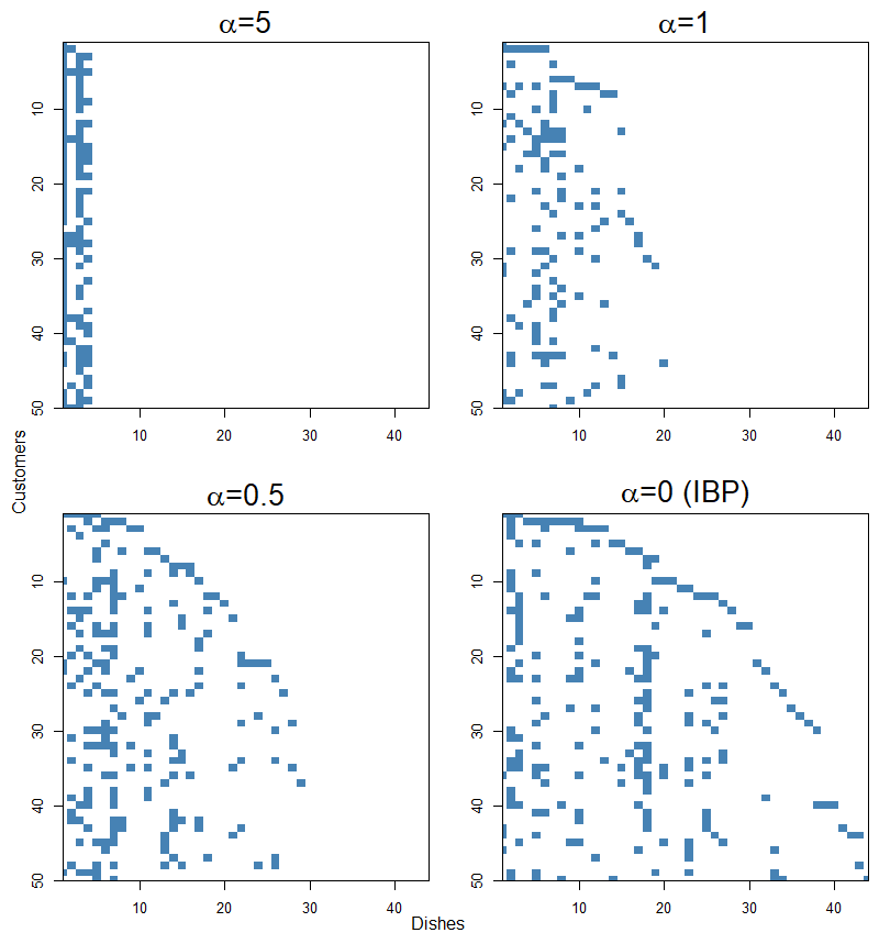
Figure 1: Draws from $\texttt{{CIBP}}(\omega\kappa/\alpha,\alpha,\kappa)$ and $\texttt{{IBP}}(\omega,\kappa)$ with $\omega=5$, $\kappa=4$ but with $\alpha=5$, $\alpha=1$ and $\alpha=0.5$.

3 Alternative representations

In this section, we provides two alternative representations of the CIBP. The first one is based on a hierarchical distribution of Poisson, Beta and Bernoulli distributions and the second one is based on random measures. The proofs of all the results in this section are deferred to Section 5.

3.1 Hierarchical representation

In this section we show that the CIBP is equivalent to the following hierarchical distribution.

Definition 2 (Hierarchical representation of the CIBP).

Let $\gamma>0$, $\alpha>0$ and $\kappa\geq 0$. We call the probability distribution given below the hierarchical representation of $\texttt{{CIBP}}(\gamma,\alpha,\kappa)$:

$$K \sim\texttt{{Poisson}}(\gamma),$$ (3.1)

$$\theta_{k} \stackrel{{\scriptstyle\textup{iid}}}{{\sim}}\texttt{{Beta}}\mathinner{\left(\alpha,\kappa+1\right)},\>k\in[K]$$

$$\xi_{jk}|\theta_{k} \stackrel{{\scriptstyle\textup{ind}}}{{\sim}}\texttt{{Bernoulli}}(\theta_{k})\>j\in[p],k\in[K].$$

To state the result rigorously, we need a concept of lof-equivalence classes. Under the latent feature model, the ordering of the features does not affect the likelihood of the data. Hence, we say that two $p\times\infty$ dimensional binary matrices are equivalent if they are identical up to a permutation of columns. It is convenient to choose a representative of every equivalence class by the left-ordering procedure. The left-ordering procedure maps each $p\times\infty$ dimensional binary matrix to its left-ordered version whose columns are ordered by the score $s_{k}$, which is defined by

$$s_{k}\mathrel{\mathop{\mathchar 58\relax}}=\sum_{j=1}^{p}\xi_{jk}2^{p-j}$$

i.e., the colums are ordered so that $s_{1}\geq s_{2}\geq\cdots.$ We call the equivalence class defined by the left-ordering procedure lof-equivalence class and we denote the lof-equivalence class of a binary matrix $\bm{\Xi}$ by $[\bm{\Xi}]$.

We introduce useful notations. Let $\Delta\mathrel{\mathop{\mathchar 58\relax}}=\{0,1\}^{p}$ which is a set of $p$-dimensional binary vectors and $\Delta_{1}\mathrel{\mathop{\mathchar 58\relax}}=\Delta\setminus\{\mathbf{0}\}$ where $\mathbf{0}$ is the vector or zero. For each $\mathbf{u}\in\Delta_{1}$, we define

$$K_{\mathbf{u}} \mathrel{\mathop{\mathchar 58\relax}}=\sum_{k=1}^{\infty}\mathbbm{1}(\bm{\xi}_{\bullet k}=\mathbf{u}),$$ (3.2)

where $\bm{\xi}_{\bullet k}$ denotes the $k$-th column of $\bm{\Xi}$. In words, $K_{\mathbf{u}}$ is the number of columns equal to the binary vector $\mathbf{u}$. Note that $K^{+}\mathrel{\mathop{\mathchar 58\relax}}=\sum_{k=1}^{\infty}\mathbbm{1}(\bm{\xi}_{\bullet k}\neq\mathbf{0})=\sum_{\mathbf{u}\in\Delta_{1}}K_{\mathbf{u}}$. Moreover, let

$$m_{k}\mathrel{\mathop{\mathchar 58\relax}}=\sum_{j=1}^{p}\xi_{jk},$$

be the number of rows that have the $k$-th feature.

In the next proposition, we provide the explicit form of the probability mass function of the lof-equivalence class $[\bm{\Xi}]$.

Proposition 3.1.

If a $p\times\infty$-dimensional random binary matrix $\Xi\equiv(\xi_{jk})_{j\in[p],k\in\mathbbm{N}}$ follows the distribution in 3.1, then

$$\mathsf{P}([\Xi])=\frac{\gamma^{K^{+}}}{\prod_{\mathbf{u}\in\Delta_{1}}K_{\mathbf{u}}!}\textup{e}^{-\gamma\sum_{j=1}^{p}\bar{\mathsf{B}}_{\alpha,\kappa+1}^{1,j-1}}\mathinner{\left[\prod_{k=1}^{K^{+}}\bar{\mathsf{B}}_{\alpha,\kappa+1}^{m_{k},p-m_{k}}\right]}.$$ (3.3)

From Proposition 3.1, we can show that the restaurant analogy and the hierarchical representation of the CIBP are equivalent.

Proposition 3.2.

Suppose that a $p\times\infty$-dimensional binary matrix $\bm{\Xi}$ follow the hierarchical distribution presented in 3.1. Then the lof-equivalence class $[\Xi]$ follows $\texttt{{CIBP}}(\gamma,\alpha,\kappa)$.

3.2 Random measure representation

In this section, we provide another representation of the CIBP, which is based on random measures.

We first briefly review completely random measures. Let $(\Omega,\mathcal{A})$ a Polish space with its Borel $\sigma$-field and let $(\mathfrak{M},\mathcal{M})$ be a set of all measures on $(\Omega,\mathcal{A})$ with its Borel $\sigma$-field. A completely random measure (CRM) $\mu$ on $(\Omega,\mathcal{A})$ is a random measure such that $\mu(A_{1}),\dots,\mu(A_{k})$ for all disjoint measurable sets $A_{1},\dots,A_{k}\in\mathcal{A}$ are mutually independent. Every CRM can be decomposed into three independent parts:

$$\mu=\mu_{0}+\sum_{k=1}^{K}q_{k}\delta_{\omega_{k}}+\sum_{(q,\omega)\in\Phi}q\delta_{\omega}$$

where $\mu_{0}$ is a non-random measure, $(\omega_{k})_{k\in[K]}$ are fixed atoms in $\Omega$, $(q_{k})_{k\in[K]}$ are independent random variables on $\mathbb{R}_{+}$ and $\Phi$ is a Poisson process on $\mathbb{R}_{+}\times\Omega$. Here we only consider purely-atomic CRMs such that $\mu_{0}=0$. We write

$$\mu\sim\texttt{{CRM}}\mathinner{\left(\Lambda,(\omega_{k},P_{k})_{k\in[K]}\right)}$$

if $\mu$ is the purely-atomic CRM represented by $\mu=\sum_{k=1}^{K}q_{k}\delta_{\omega_{k}}+\sum_{(q,\omega)\in\Phi}q\delta_{\omega}$ with $q_{k}\stackrel{{\scriptstyle\textup{ind}}}{{\sim}}P_{k}$ for $k\in[K]$ and $\mathsf{E}\Phi=\Lambda$ for some probability measures $(P_{k})_{k\in[K]}$ on $\mathbb{R}_{+}$ and $\Lambda$ on $\mathbb{R}_{+}\times\Omega$. In particular, we write $\mu\sim\texttt{{CRM}}\mathinner{\left(\Lambda\right)}$ if $\mu=\sum_{(q,\omega)\in\Phi}q\delta_{\omega}$ with $\mathsf{E}\Phi=\Lambda$.

It is well known that the two-parameter IBP, $\texttt{{IBP}}(\alpha,\kappa+1)$ with $\alpha>0$ and $\kappa\geq 0$, has the following random measure representation:

$$\bm{\xi}_{j\bullet}|\mu \stackrel{{\scriptstyle\textup{iid}}}{{\sim}}\texttt{{BeP}}(\mu),\>j\in[p]$$

$$\mu \sim\texttt{{BP}}(\kappa+1,\alpha\Lambda_{0})$$

for some smooth probability measure $\Lambda_{0}$, i.e., $\Lambda_{0}(\Omega)=1$. Here, $\texttt{{BeP}}(\mu)$ denotes the Bernoulli process with mean $\mu$, which is equivalent to $\texttt{{CRM}}(\Lambda_{\texttt{{BeP}}(\mu)})$ on $(\Omega,\mathcal{A})$ with

$$\Lambda_{\texttt{{BeP}}(\mu)}(\textup{d}q,\textup{d}\omega)=\delta_{1}(\textup{d}q)\mu(\textup{d}\omega),$$

where $\delta_{1}$ denotes a point mass at 1, and $\texttt{{BP}}(\kappa+1,\alpha\Lambda_{0})$ denotes the Beta process which is equivalent to $\texttt{{CRM}}(\Lambda_{\textup{BP}(\theta,\gamma\Lambda_{0})})$ on $(\Omega,\mathcal{A})$ with

$$\Lambda_{\texttt{{BP}}(\kappa+1,\alpha\Lambda_{0})}(\textup{d}q,\textup{d}\omega)=\alpha(\kappa+1)q^{-1}(1-q)^{\kappa}\textup{d}q\Lambda_{0}(\textup{d}\omega).$$

We introduce another stochastic process represented by a random measure, which will be shown to be related to the CIBP.

Definition 3 (Random measure representation of the CIBP).

Let $\gamma>0$, $\alpha>0$ and $\kappa\geq 0$. We call the stochastic process given below the random measure representation of $\texttt{{CIBP}}(\gamma,\alpha,\kappa)$:

$$\bm{\xi}_{j\bullet}|\mu \stackrel{{\scriptstyle\textup{iid}}}{{\sim}}\texttt{{BeP}}(\mu),\>j\in[p]$$ (3.4)

$$\mu \sim\texttt{{CRM}}(\Lambda_{\texttt{{CIBP}}(\gamma,\alpha,\kappa)})$$

with

$$\Lambda_{\texttt{{CIBP}}(\gamma,\alpha,\kappa)}(\textup{d}q,\textup{d}\omega)=\frac{\gamma}{\mathsf{B}(\alpha,\kappa+1)}q^{\alpha-1}(1-q)^{\kappa}\textup{d}q\Lambda_{0}(\textup{d}\omega)$$ (3.5)

for some smooth probability measure $\Lambda_{0}$.

The next theorem shows that the hierarchical representation in Definition 2 and random measure representation in Definition 3 of the CIBP are equivalent.

Proposition 3.3.

Let $\bm{\xi}_{1\bullet},\dots,\bm{\xi}_{p\bullet}$ be random measures following the distribution given in 3.4. Then the joint distribution of $\bm{\xi}_{1\bullet},\dots,\bm{\xi}_{p\bullet}$ is given by

$$\mathsf{P}(\bm{\xi}_{1\bullet},\dots,\bm{\xi}_{p\bullet})=\textup{e}^{-\gamma\sum_{j=1}^{p}\bar{\mathsf{B}}_{\alpha,\kappa+1}^{1,j-1}}\mathinner{\left[\prod_{k=1}^{K^{+}}\bar{\mathsf{B}}_{\alpha,\kappa+1}^{m_{k},p-m_{k}}\lambda_{0}(\omega_{k}^{*})\right]},$$ (3.6)

where there are $K^{+}$ atoms $\omega_{1}^{*},\cdots,\omega_{K^{+}}^{*}$ such that $m_{k}\mathrel{\mathop{\mathchar 58\relax}}=\sum_{j=1}^{p}\bm{\xi}_{j\bullet}(\omega_{k}^{*})\geq 1$ for $k\in[K^{+}]$, and $\lambda_{0}$ denotes the density of $\Lambda_{0}$.

The function $q\mapsto q^{\alpha-1}(1-q)^{\kappa}$ is integrable on $[0,1]$, which means that there would be a finite number of features.

4 Application to Bayesian sparse factor models

In this section, we consider an application of the CIBP prior distribution to Bayesian estimation of the factor model.

4.1 Model and prior

We consider the following factor model where a $p$-dimensional random vector $\mathbf{Y}$ is distributed as

$$\mathbf{Y}|\mathbf{Z}=\mathbf{z}\sim\texttt{{N}}_{p}(\mathbf{B}\mathbf{z},\sigma^{2}\mathbf{I}),\quad\mathbf{Z}\sim\texttt{{N}}_{K}(\mathbf{0},\mathbf{I}),$$ (4.1)

with $K<p$, $\mathbf{B}$ being a $p\times K$ factor loading matrix, $\mathbf{Z}$ a $K$-dimensional factor and $\sigma^{2}>0$ a noise variance.

We consider the following prior on the loading matrix $\mathbf{B}$. Let $\beta_{jk}$ be the $(j,k)$-th entry of the $p\times\infty$-dimensional loading matrix $\mathbf{B}$. We impose the prior distribution based on the CIBP distribution such that

$$\beta_{jk}|\xi_{jk}\stackrel{{\scriptstyle\textup{ind}}}{{\sim}} (1-\xi_{jk})\delta_{0}+\xi_{jk}\texttt{{N}}(0,\tau),\>j\in[p],\>k\in[K]$$

$$\xi_{jk}|\theta_{k}\stackrel{{\scriptstyle\textup{ind}}}{{\sim}} \texttt{{Bernoulli}}\mathinner{\left(\theta_{k}\right)},\>j\in[p],\>k\in[K]$$

$$\theta_{k}\stackrel{{\scriptstyle\textup{iid}}}{{\sim}} \texttt{{Beta}}(\alpha,\kappa+1),\>k\in[K]$$

$$K\sim \texttt{{Poisson}}(\gamma)$$

where $\kappa\geq 0$ and $\tau>0$. That is, we impose $\texttt{{CIBP}}(\gamma,\alpha,\kappa)$ on the binary matrix $\bm{\Xi}\mathrel{\mathop{\mathchar 58\relax}}=(\xi_{jk})_{j\in[p],k\in\mathbbm{N}}$. We refer to the above distribution on $\mathbf{B}$ as $\mathsf{SSCIBP}_{p}(\gamma,\alpha,\kappa,\tau)$, which is an abbreviation of spike and slab CIBP.

4.2 Posterior computation

We provide an Markov chain Monte Carlo (MCMC) algorithm for sampling from the posterior distribution under the $\mathsf{SSCIBP}_{p}(\gamma,\alpha,\kappa,\tau)$ prior on $\mathbf{B}$ and inverse Gamma prior $\texttt{{IG}}(a,b)$ on $\sigma^{2}$. Let $K^{+}$ be the number of nonzero columns of the loading matrix $\mathbf{B}$. The MCMC algorithm is as follows:

Sample $\beta_{jk}$ for $j\in[p]$ and $k\in[K^{+}]$.

The factor loading $\beta_{jk}$ is sampled from the conditional posterior

$$\beta_{jk}|-\sim\begin{cases}\texttt{{N}}(\widehat{\beta}_{jk},\widehat{\tau}_{k})&\mbox{if }\xi_{jk}=1\\ \delta_{0}&\mbox{if }\xi_{jk}=0,\end{cases}$$

where

$$\widehat{\tau}_{k} \mathrel{\mathop{\mathchar 58\relax}}=\mathinner{\left(\sigma^{-2}\sum_{i=1}^{n}Z_{ik}^{2}+\tau^{-1}\right)}^{-1}$$

$$\widehat{\beta}_{jk} \mathrel{\mathop{\mathchar 58\relax}}=\widehat{\tau}_{k}\mathinner{\left\{\sigma^{-2}\sum_{i=1}^{n}Z_{ik}\mathinner{\left(Y_{ij}-\sum_{h\in[K^{+}]\mathrel{\mathop{\mathchar 58\relax}}h\neq k}Z_{ih}\beta_{jh}\right)}\right\}}.$$

Sample $\xi_{jk}$ for $j\in[p]$ and $k\in\mathbbm{N}$.

When we sample $(\xi_{jk}\mathrel{\mathop{\mathchar 58\relax}}k\in\mathbbm{N})$, we use the fact that the CIBP is exchangeable to assume that the $j$-th customer is the last customer to enter the restaurant. Therefore, for each $k\in[K^{*}]$, $\xi_{jk}$ is sampled with probability

$$\frac{\Pi(\xi_{jk}=1|-)}{\Pi(\xi_{jk}=0|-)}=\frac{m_{j,k}+\alpha}{\kappa+p-m_{j,k}}\sqrt{\frac{\widehat{\tau}_{k}}{\tau}}\exp\mathinner{\left(\frac{1}{2\widehat{\tau}_{k}}\widehat{\beta}_{jk}^{2}\right)},$$

where $m_{j,k}\mathrel{\mathop{\mathchar 58\relax}}=\sum_{l\in[p]\mathrel{\mathop{\mathchar 58\relax}}l\neq j}\xi_{lk}$. We then sample $\xi_{jk}$ for each of the infinitely many all-zero columns. To do this, we use the Metropolis–Hastings (MH) steps as follows. We propose $K_{j}^{*}\in\mathbbm{N}\cup\{0\}$ and $\bm{\beta}_{j}^{*}\mathrel{\mathop{\mathchar 58\relax}}=(\beta_{j,1}^{*},\dots,\beta_{j,K_{j}^{*}}^{*})\in\mathbb{R}^{K_{j}^{*}}$ from the proposal distribution

$$J(K_{j}^{*})J(\beta_{j}^{*}|K_{j}^{*})=\texttt{{Poisson}}(1)\texttt{{N}}(0,\tau)^{K_{j}^{*}}.$$

Then we accept the proposal with probability

$$\min\mathinner{\left\{1,\mathinner{\lvert\mathbf{M}_{j}\rvert}^{-n/2}\exp\mathinner{\left(\frac{1}{2}(\bm{\beta}_{j}^{*})^{\top}\mathbf{M}_{j}^{-1}\bm{\beta}_{j}^{*}\sum_{i=1}^{n}E_{ij}^{2}\right)}\mathinner{\left(\gamma\bar{\mathsf{B}}^{1,p-1}_{\alpha,\kappa+1}\right)}^{K_{j}^{*}}\right\}},$$

where

$$\mathbf{M}_{j} \mathrel{\mathop{\mathchar 58\relax}}=\sigma^{-2}\bm{\beta}_{j}^{*}(\bm{\beta}_{j}^{*})^{\top}+\mathbf{I}$$

$$E_{ij} \mathrel{\mathop{\mathchar 58\relax}}=\sigma^{-2}\mathinner{\left(Y_{ij}-\sum_{k=1}^{K^{+}}Z_{ik}\beta_{jk}\right)}.$$

If the proposal is accepted, we update

$$\mathbf{B} \leftarrow(\mathbf{B},(\beta_{j,k}^{*}\mathbbm{1}(l=j))_{l\in[p],k\in[K_{j}^{*}]})$$

$$K^{+} \leftarrow K^{+}+K_{j}^{*}.$$

Sample $\mathbf{Z}_{i}$ for $i\in[n]$.

The latent variable $\mathbf{Z}_{i}$ is sampled from

$$\mathbf{Z}_{i}|-\sim\texttt{{N}}\mathinner{\left(\sigma^{-2}\widehat{\bm{\Sigma}}_{\mathbf{Z}}\mathbf{B}^{\top}\mathbf{Y}_{i},\widehat{\bm{\Sigma}}_{\mathbf{Z}}\right)}$$

where $\widehat{\bm{\Sigma}}_{\mathbf{Z}}\mathrel{\mathop{\mathchar 58\relax}}=(\sigma^{-2}\mathbf{B}^{\top}\mathbf{B}+\mathbf{I})^{-1}$.

Sample $\sigma^{2}$.

The noise variance $\sigma^{2}$ is sampled from

$$\sigma^{2}|-\sim\texttt{{IG}}\mathinner{\left(a+\frac{np}{2},b+\frac{1}{2}\sum_{i=1}^{n}\sum_{j=1}^{p}\mathinner{\left(Y_{ij}-\sum_{k=1}^{K^{+}}Z_{ik}\beta_{jk}\right)}^{2}\right)}.$$

4.3 Simulation

We conduct simulation to compare the CIBP and the two-parameter IBP when they are used as prior distributions for the sparse factor model.

We generate simulated data sets as follows. For each value $p\in\{50,100,150,\dots,300\}$, we generate a $p\times 4$-dimensional loading matrix $\mathbf{B}_{0}$ with the number of nonzero rows $10$. The loadings in the sampled nonzero rows are generated from the uniform distribution on $(-3,-2)\cup(2,3)$. Then we sample $n=50$ random vectors from the multivariate normal distribution with mean $\mathbf{0}$ and variance $\mathbf{B}_{0}(\mathbf{B}_{0})^{\top}+\mathbf{I}$ independently. We repeat this generating procedure 100 times.

For each synthetic data set, we compute the posterior distribution under the $\texttt{{CIBP}}(\gamma,\alpha,\kappa)$ and $\texttt{{IBP}}(\omega,\kappa)$ prior, respectively. For the CIBP prior, we set $\gamma=1$, $\alpha=10$ and $\kappa=10$. For the IBP prior, we set $\omega=1$ which is equal to $\gamma\alpha/\kappa$. In Figure 2, we present the posterior mean of the number of factors under the $\texttt{{CIBP}}(\gamma,\alpha,\kappa)$ and $\texttt{{IBP}}(\omega,\kappa)$ prior, respectively, for $p\in\{50,100,150,\dots,300\}$ over 100 replications. As the dimension $p$ increases, the $\texttt{{IBP}}(\omega,\kappa)$ prior tends to more largely overestimate the number of factors. But the $\texttt{{CIBP}}(\gamma,\alpha,\kappa)$ prior provides accurate estimates of the number of factors for all the values of $p.$

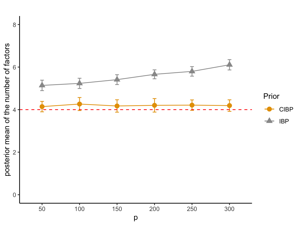
Figure 2: The posterior mean of the number of factors under the $\texttt{{CIBP}}(\gamma,\alpha,\kappa)$ and $\texttt{{IBP}}(\omega,\kappa)$ priors. The red dashed line indicates the true number of factors, 4.

5 Proofs for Section 3

5.1 Proof of Proposition 3.1

Proof.

Recall that $m_{k}\mathrel{\mathop{\mathchar 58\relax}}=\sum_{j=1}^{p}\xi_{jk}$. If $K\geq K^{+}$, we have that

$$\mathsf{P}(\bm{\Xi}|K) =\prod_{k=1}^{K}\frac{\mathsf{B}(m_{k}+\alpha,p-m_{k}+\kappa+1)}{\mathsf{B}(\alpha,\kappa+1)}$$

$$=\mathinner{\left(\frac{\mathsf{B}(\alpha,p+\kappa+1)}{\mathsf{B}(\alpha,\kappa+1)}\right)}^{K-K^{+}}\prod_{k=1}^{K^{+}}\frac{\mathsf{B}(m_{k}+\alpha,p-m_{k}+\kappa+1)}{\mathsf{B}(\alpha,\kappa+1)}$$

$$=\mathinner{\left(\bar{\mathsf{B}}_{\alpha,\kappa+1}^{0,p}\right)}^{K-K^{+}}\prod_{k=1}^{K^{+}}\bar{\mathsf{B}}_{\alpha,\kappa+1}^{m_{k},p-m_{k}},$$

where the second equality follows from reordering the columns such that $m_{k}>0$ if $k\leq K^{+}$ and $m_{k}=0$ otherwise. Recall that $\bar{\mathsf{B}}_{a_{1},b_{1}}^{a_{2},b_{2}}=\mathsf{B}(a_{1}+a_{2},b_{1}+b_{2})/\mathsf{B}(a_{1},b_{1})$. Therefore, since the cardinality of the lof-equivalence class is $|[\bm{\Xi}]]=K!/\prod_{\mathbf{u}\in\Delta}K_{\mathbf{u}}!$, the probability of a lof equivalence class of $\bm{\Xi}$ given $K\geq K^{+}$ is given by

$$\mathsf{P}([\bm{\Xi}]|K)=\frac{K!}{\prod_{\mathbf{u}\in\Delta}K_{\mathbf{u}}!}\mathinner{\left(\bar{\mathsf{B}}_{\alpha,\kappa+1}^{0,p}\right)}^{K-K^{+}}\prod_{k=1}^{K^{+}}\bar{\mathsf{B}}_{\alpha,\kappa+1}^{m_{k},p-m_{k}}$$

If $K<K^{+}$, it is clear that $\mathsf{P}(\bm{\Xi}|K)=0$.

Let $p_{K}$ the probability mass function of $\texttt{{Poisson}}(\gamma)$, i.e., $p_{K}(k)\mathrel{\mathop{\mathchar 58\relax}}=\textup{e}^{-\gamma}\gamma^{k}/k!$ for $k\in\mathbbm{N}$. Marginalizing over $K$, we have that

$$\mathsf{P}([\bm{\Xi}])=\frac{1}{\prod_{\mathbf{u}\in\Delta_{1}}K_{\mathbf{u}}!}\mathinner{\left[\prod_{k=1}^{K^{+}}\bar{\mathsf{B}}_{\alpha,\kappa+1}^{m_{k},p-m_{k}}\right]}\sum_{K=K^{+}}^{\infty}\frac{K!}{K_{\mathbf{0}}!}\mathinner{\left(\bar{\mathsf{B}}_{\alpha,\kappa+1}^{0,p}\right)}^{K-K^{+}}p_{K}(K).$$

The summation term of the preceding display can be written as

$$\sum_{K=K_{+}}^{\infty}\frac{K!}{K_{\mathbf{0}}!}\mathinner{\left(\bar{\mathsf{B}}_{\alpha,\kappa+1}^{0,p}\right)}^{K-K^{+}}p_{K}(k) =\textup{e}^{-\gamma}\gamma^{K^{+}}\sum_{K=K_{+}}^{\infty}\frac{1}{(K-K^{+})!}\mathinner{\left(\gamma\bar{\mathsf{B}}_{\alpha,\kappa+1}^{0,p}\right)}^{K-K^{+}}$$ (5.1)

$$=\gamma^{K^{+}}\textup{e}^{-\gamma\mathinner{\left(1-\bar{\mathsf{B}}_{\alpha,\kappa+1}^{0,p}\right)}},$$

where we use the identity $\textup{e}^{x}=\sum_{k=0}^{\infty}x^{k}/k!$ for the second inequality. Lastly, from the identity $\mathsf{B}(x,y)-\mathsf{B}(x,y+1)=\mathsf{B}(x+1,y)$, it follows that

$$1-\bar{\mathsf{B}}_{\alpha,\kappa+1}^{0,p} =1-\frac{\mathsf{B}(\alpha,p+\kappa+1)}{\mathsf{B}(\alpha,\kappa+1)}$$ (5.2)

$$=\frac{1}{\mathsf{B}(\alpha,\kappa+1)}\mathinner{\left\{\mathsf{B}(\alpha,\kappa+1)-\mathsf{B}(\alpha,p+\kappa+1)\right\}}$$

$$=\frac{1}{\mathsf{B}(\alpha,\kappa+1)}\sum_{j=1}^{p}\mathinner{\left\{\mathsf{B}(\alpha,\kappa+j)-\mathsf{B}(\alpha,\kappa+j+1)\right\}}$$

$$=\frac{1}{\mathsf{B}(\alpha,\kappa+1)}\sum_{j=1}^{p}\mathsf{B}(\alpha+1,\kappa+j)$$

$$=\sum_{j=1}^{p}\bar{\mathsf{B}}_{\alpha,\kappa+1}^{1,j-1}.$$

Combining 5.1 and 5.2, we get the desired result. ∎

5.2 Proof of Proposition 3.2

Proof.

The proof is by induction. Let $\bm{\xi}_{j\bullet}$ be the $j$-th row of $\bm{\Xi}$. For $p=1$, from a Poisson likelihood, we have

$$\mathsf{P}(\bm{\xi}_{1\bullet})=\frac{1}{K_{1}^{+}!}\mathinner{\left(\gamma\bar{\mathsf{B}}_{\alpha,\kappa+1}^{1,0}\right)}^{K_{1}^{+}}\textup{e}^{-\gamma\bar{\mathsf{B}}_{\alpha,\kappa+1}^{1,0}}$$

where $K_{1}^{+}$ is a number of nonzero elements of $\bm{\xi}_{1\bullet}$. It is same as 3.3 with $p=1$ and $K^{+}=K_{1}^{+}$.

For $p\geq 2$, consider the conditional distribution of $\bm{\xi}_{p\bullet}$ given $\bm{\xi}_{1\bullet},\dots,\bm{\xi}_{p-1\bullet}$, which is given by

$$\mathsf{P}(\bm{\xi}_{p\bullet}|\bm{\xi}_{1\bullet},\dots,\bm{\xi}_{p-1\bullet}) =\textup{e}^{-\gamma\bar{\mathsf{B}}_{\alpha,\kappa+1}^{1,p-1}}\frac{(\gamma\bar{\mathsf{B}}_{\alpha,\kappa+1}^{1,p-1})^{K^{\textup{new}}_{p}}}{K^{\textup{new}}_{p}!}$$ (5.3)

$$\quad\times\prod_{k\in J_{p}}\frac{m_{p,k}+\alpha}{p+\kappa+\alpha}\prod_{k\notin J_{p}}\frac{p-m_{p,k}+\kappa}{p+\kappa+\alpha},$$

where $m_{p,k}\mathrel{\mathop{\mathchar 58\relax}}=\sum_{j=1}^{p-1}\xi_{jk}$, $K^{\textup{new}}_{p}$ is the number of new features sampled by the $p$-th customer and $J_{p}$ is the set of dishes taken by the $p$-th customer, i.e., $J_{p}\mathrel{\mathop{\mathchar 58\relax}}=\mathinner{\left\{k\in[K_{p-1}^{+}]\mathrel{\mathop{\mathchar 58\relax}}\xi_{pk}=1\right\}}$. Let $K_{p}^{+}\mathrel{\mathop{\mathchar 58\relax}}=\sum_{j=1}^{p}K^{\textup{new}}_{j}=K_{p-1}^{+}+K^{\textup{new}}_{p}$ and $K^{\textup{new}}_{1}=K_{1}^{+}$. By the inductive hypothesis, we have

$$\mathsf{P}(\bm{\xi}_{1\bullet},\dots,\bm{\xi}_{p\bullet}) =\mathsf{P}(\bm{\xi}_{p\bullet}|\bm{\xi}_{1\bullet},\dots,\bm{\xi}_{p-1\bullet})\mathsf{P}(\bm{\xi}_{1\bullet},\dots,\bm{\xi}_{p-1\bullet})$$

$$=\textup{e}^{-\gamma\sum_{j=1}^{p}\bar{\mathsf{B}}_{\alpha,\kappa+1}^{0,j-1}}\frac{\gamma^{K_{p}^{+}}}{\prod_{j=1}^{p}K^{\textup{new}}_{j}!}\prod_{k\in J_{p}}\frac{m_{p,k}+\alpha}{p+\kappa+\alpha}\bar{\mathsf{B}}_{\alpha,\kappa+1}^{m_{p,k},p-1-m_{p,k}}$$

$$\quad\times\prod_{k\notin J_{p}}\frac{p-m_{p,k}}{p+\kappa+\alpha}\bar{\mathsf{B}}_{\alpha,\kappa+1}^{m_{p,k},p-1-m_{p,k}}\times\mathinner{\left(\bar{\mathsf{B}}_{\alpha,\kappa+1}^{1,p-1}\right)}^{K^{\textup{new}}_{p}}$$

Since $m_{k}=m_{p,k}+1$ for $k\in J_{p}$ and $m_{k}=m_{p,k}$ otherwise, we have

$$\frac{m_{p,k}+\alpha}{p+\kappa+\alpha}\bar{\mathsf{B}}_{\alpha,\kappa+1}^{m_{p,k},p-1-m_{p,k}} =\frac{m_{p,k}+\alpha}{p+\kappa+\alpha}\frac{\mathsf{B}(m_{p,k}+\alpha,p-m_{p,k}+\kappa)}{\mathsf{B}(\alpha,\kappa+1)}$$

$$=\frac{\mathsf{B}(m_{p,k}+1+\alpha,p-m_{p,k}+\kappa)}{\mathsf{B}(\alpha,\kappa+1)}$$

$$=\bar{\mathsf{B}}_{\alpha,\kappa+1}^{m_{p,k}+1,p-1-m_{p,k}}$$

$$=\bar{\mathsf{B}}_{\alpha,\kappa+1}^{m_{k},p-m_{k}}$$

and similarly,

$$\frac{p-m_{p,k}}{p+\kappa+\alpha}\bar{\mathsf{B}}_{\alpha,\kappa+1}^{m_{p,k},p-1-m_{p,k}}=\bar{\mathsf{B}}_{\alpha,\kappa+1}^{m_{p,k},p-m_{p,k}}=\bar{\mathsf{B}}_{\alpha,\kappa+1}^{m_{k},p-m_{k}}.$$

Therefore,

$$\mathsf{P}(\bm{\xi}_{1\bullet},\dots,\bm{\xi}_{p\bullet}) =\textup{e}^{-\gamma\sum_{j=1}^{p}\bar{\mathsf{B}}_{\alpha,\kappa+1}^{1,j-1}}\frac{\gamma^{K_{p}^{+}}}{\prod_{j=1}^{p}K^{\textup{new}}_{j}!}\prod_{k\in J_{p}}\bar{\mathsf{B}}_{\alpha,\kappa+1}^{m_{k},p-m_{k}}$$ (5.4)

$$\quad\times\prod_{k\notin J_{p}}\bar{\mathsf{B}}_{\alpha,\kappa+1}^{m_{k},p-m_{k}}\times\mathinner{\left(\bar{\mathsf{B}}_{\alpha,\kappa+1}^{1,p-1}\right)}^{K^{\textup{new}}_{p}}$$

$$=\textup{e}^{-\gamma\sum_{j=1}^{p}\bar{\mathsf{B}}_{\alpha,\kappa+1}^{1,j-1}}\frac{\gamma^{K_{p}^{+}}}{\prod_{j=1}^{p}K^{\textup{new}}_{j}!}\prod_{k=1}^{K_{p}^{+}}\bar{\mathsf{B}}_{\alpha,\kappa+1}^{m_{k},p-m_{k}}.$$

Note that $\prod_{j=1}^{p}K^{\textup{new}}_{j}!/\prod_{\mathbf{u}\in\Delta_{1}}K_{\mathbf{u}}$ matrices generated by the above process have the same left-ordered form, hence $\mathsf{P}([\bm{\Xi}])$ is obtained by multiplying $\mathsf{P}(\bm{\xi}_{1\bullet},\dots,\bm{\xi}_{p\bullet})$ in 5.4 by this quantity. ∎

5.3 Proof of Proposition 3.3

Proof.

By the well-known conjugacy result (Theorem 3.3 of Kim et al., [3]),

$$\mu|\bm{\xi}_{1\bullet},\dots,\bm{\xi}_{p-1\bullet}\sim\texttt{{CRM}}(\Lambda_{p},\{\omega_{k}^{*},P_{k}\}_{k=1}^{K}),$$

where $\omega_{1}^{*},\dots,\omega_{K}^{*}$ are unique atoms that $\bm{\xi}_{1\bullet},\dots,\bm{\xi}_{p-1\bullet}$ possess,

$$P_{k}(\textup{d}q) \mathrel{\mathop{\mathchar 58\relax}}=\frac{q^{m_{p,k}+\alpha-1}(1-q)^{p-1-m_{p,k}+\kappa}\textup{d}q}{\int_{(0,1]}q^{m_{p,k}+\alpha-1}(1-q)^{p-1-m_{p,k}+\kappa}\textup{d}q}$$

$$=\frac{1}{\mathsf{B}(m_{p,k}+\alpha,p-m_{p,k}+\kappa)}q^{m_{p,k}+\alpha-1}(1-q)^{p-1-m_{p,k}+\kappa}\textup{d}q,$$

with $m_{p,k}\mathrel{\mathop{\mathchar 58\relax}}=\sum_{j=1}^{p-1}\bm{\xi}_{j\bullet}(\omega_{k}^{*})$, and

$$\Lambda_{p}(\textup{d}q,\textup{d}\omega)\mathrel{\mathop{\mathchar 58\relax}}=\frac{\gamma}{\mathsf{B}(\alpha,\kappa+1)}q^{\alpha-1}(1-q)^{p-1+\kappa}\textup{d}q\Lambda_{0}(\textup{d}\omega).$$

Thus, for each atom $\omega_{k}^{*}$, we have that

$$\mathsf{P}\mathinner{\left(\bm{\xi}_{p\bullet}(\omega_{k}^{*})=1|\bm{\xi}_{1\bullet},\dots,\bm{\xi}_{p-1\bullet}\right)}$$ (5.5)

$$=\frac{1}{\mathsf{B}(m_{p,k}+\alpha,p-m_{p,k}+\kappa)}\int_{(0,1]}q^{m_{p,k}+\alpha}(1-q)^{p-1-m_{p,k}+\kappa}\textup{d}q$$

$$=\frac{1}{\mathsf{B}(m_{p-1,k}+\alpha,p-m_{p-1,k}+\kappa)}{\mathsf{B}(m_{p,k}+1+\alpha,p-m_{p,k}+\kappa)}$$

$$=\frac{m_{p,k}+\alpha}{p+\kappa+\alpha}.$$

On the other hand, for a small neighborhood $\textup{d}\omega$ around $\omega\in\Omega\setminus\{\omega_{1}^{*},\dots,\omega_{K}^{*}\}$, we have

$$\mathsf{P}\mathinner{\left(\bm{\xi}_{p\bullet}(\textup{d}\omega)=1|\bm{\xi}_{1\bullet},\dots,\bm{\xi}_{p-1\bullet}\right)}$$ (5.6)

$$=\mathsf{E}\mathinner{\left[\bm{\xi}_{p\bullet}(\textup{d}\omega)|\bm{\xi}_{1\bullet},\dots,\bm{\xi}_{p-1\bullet}\right]}$$

$$=\frac{\gamma}{\mathsf{B}(\alpha,\kappa+1)}\int_{(0,1]}q^{\alpha}(1-q)^{p-1+\kappa}\textup{d}q\Lambda_{0}(\textup{d}\omega)$$

$$=\gamma\frac{\mathsf{B}(\alpha+1,p+\kappa)}{\mathsf{B}(\alpha,\kappa+1)}\Lambda_{0}(\textup{d}\omega)$$

$$=\gamma\bar{\mathsf{B}}_{\alpha,\kappa+1}^{1,p-1}\Lambda_{0}(\textup{d}\omega)$$

This implies that on $\Omega\setminus\{\omega_{1}^{*},\dots,\omega_{K}^{*}\}$, $\bm{\xi}_{p\bullet}$ is a Poisson process with intensity measure $\gamma\bar{\mathsf{B}}_{\alpha,\kappa+1}^{1,p-1}\Lambda_{0}$, since $\bm{\xi}_{p\bullet}$ is completely random and $\Lambda_{0}$ is smooth. Thus, the number of new atoms in $\bm{\xi}_{p\bullet}$ follows Poisson distribution with rate $\gamma\bar{\mathsf{B}}_{\alpha,\kappa+1}^{1,p-1}$. Combining LABEL:eq:crm_prev_dish and LABEL:eq:crm_new_dish, we complete the proof. ∎

6 Conclusion

In this paper, we proposed the CIBP, a new three-parameter generalization of the IBP. The most notable property of the CIBP compared with the standard IBPs is that the distribution of the number of features converges to a fixed distribution as the number of objects grows. Due to this property, the CIBP prevents features that are unnecessary in interpretation and/or prediction. The proposed CIBP is assessed on a high-dimensional sparse factor model. We provided empirical evidence showing that the CIBP is better than the IBP in estimation of the number of factors.

Acknowledgement

This work was supported by INHA UNIVERSITY Research Grant.

References

• Caron, [2012] Caron, F. (2012). Bayesian nonparametric models for bipartite graphs. In Advances in Neural Information Processing Systems, pages 2051–2059.
• Griffiths and Ghahramani, [2005] Griffiths, T. L. and Ghahramani, Z. (2005). Infinite latent feature models and the indian buffet process. In Proceedings of the 18th International Conference on Neural Information Processing Systems, pages 475–482.
• Kim et al., [1999] Kim, Y. et al. (1999). Nonparametric bayesian estimators for counting processes. The Annals of Statistics, 27(2):562–588.
• Meeds et al., [2007] Meeds, E., Ghahramani, Z., Neal, R. M., and Roweis, S. T. (2007). Modeling dyadic data with binary latent factors. In Advances in Neural Information Processing Systems, pages 977–984.
• Miller et al., [2009] Miller, K., Jordan, M. I., and Griffiths, T. L. (2009). Nonparametric latent feature models for link prediction. In Advances in Neural Information Processing Systems, pages 1276–1284.
• Navarro and Griffiths, [2008] Navarro, D. J. and Griffiths, T. L. (2008). Latent features in similarity judgments: A nonparametric bayesian approach. Neural computation, 20(11):2597–2628.
• Onatski, [2010] Onatski, A. (2010). Determining the number of factors from empirical distribution of eigenvalues. The Review of Economics and Statistics, 92(4):1004–1016.
• Teh and Gorur, [2009] Teh, Y. W. and Gorur, D. (2009). Indian buffet processes with power-law behavior. In Advances in Neural Information Processing Systems, pages 1838–1846.
• Thibaux and Jordan, [2007] Thibaux, R. and Jordan, M. I. (2007). Hierarchical beta processes and the indian buffet process. In Artificial Intelligence and Statistics, pages 564–571.