Joint Class-Affinity Loss Correction for Robust Medical Image Segmentation with Noisy Labels

Abstract

Noisy labels collected with limited annotation cost prevent medical image segmentation algorithms from learning precise semantic correlations. Previous segmentation arts of learning with noisy labels merely perform a pixel-wise manner to preserve semantics, such as pixel-wise label correction, but neglect the pair-wise manner. In fact, we observe that the pair-wise manner capturing affinity relations between pixels can greatly reduce the label noise rate. Motivated by this observation, we present a novel perspective for noisy mitigation by incorporating both pixel-wise and pair-wise manners, where supervisions are derived from noisy class and affinity labels, respectively. Unifying the pixel-wise and pair-wise manners, we propose a robust Joint Class-Affinity Segmentation (JCAS) framework to combat label noise issues in medical image segmentation. Considering the affinity in pair-wise manner incorporates contextual dependencies, a differentiated affinity reasoning (DAR) module is devised to rectify the pixel-wise segmentation prediction by reasoning about intra-class and inter-class affinity relations. To further enhance the noise resistance, a class-affinity loss correction (CALC) strategy is designed to correct supervision signals via the modeled noise label distributions in class and affinity labels. Meanwhile, CALC strategy interacts the pixel-wise and pair-wise manners through the theoretically derived consistency regularization. Extensive experiments under both synthetic and real-world noisy labels corroborate the efficacy of the proposed JCAS framework with a minimum gap towards the upper bound performance. The source code is available at https://github.com/CityU-AIM-Group/JCAS.

1 Introduction

Image segmentation, as one of the most essential tasks in medical image analysis, has received lots of attention over the last decades. This task aims to assign a semantic label for each pixel, further benefiting various clinical applications such as treatment planning and surgical navigation [9]. Deep learning algorithms based on convolutional neural networks (CNNs) have achieved remarkable progress in medical image segmentation, but they require a large amount of training data with precise pixel-level annotations that are extremely expensive and labor-intensive to obtain [10]. With limited budgets and efforts, the resulting dataset would be noisy, and the presence of label noises may mislead the segmentation model to memorize wrong semantic correlations, resulting in severely degraded generalizability [8, 23]. Hence, developing medical image segmentation techniques that are robust to noisy labels in training data is of great importance.

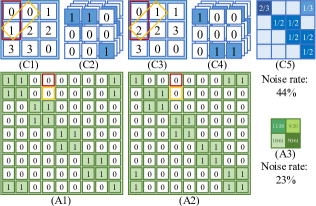
Figure 1: A toy example to illustrate the comparison between pixel-wise class label (C) and pair-wise affinity label (A). (C1, C2) True class label and the one-hot encoding. (C3, C4) Noisy class label and the one-hot encoding. (C5) Class-level noise transition matrix with noise rate of 44%. (A1) True affinity label. (A2) Noisy affinity label. (A3) Affinity-level noise transition matrix with noise rate of 23%.

Solutions towards noisy label issues in image classification tasks have been extensively explored [11, 15, 17, 22, 23], while pixel-wise label noises in segmentation tasks have not been well-studied, especially for medical image analysis. Previous solutions for medical image segmentation with noisy labels can be summarized into three aspects. Firstly, some researchers model the noisy label distribution through either the confusion matrix [20] or noise transition matrix (NTM) [6, 7], and then leverage the modeled distribution for pixel-wise loss corrections. Secondly, pixel-wise label refurbishments are implemented by the spatial label smoothing regularization [19] or the convex combination with superpixel predictions [10]. Thirdly, pixel-wise resampling and reweighting strategies are designed to concentrate the segmentation model on learning reliable pixels. For instance, Tri-network et al. [21] contains three collaborative networks and adaptively selects informative samples according to the consensus between predictions from different networks. Wang et al. [16] leverage meta-learning to automatically estimate an importance map, thereby mining reliable information from important pixels.

Despite the impressive performance in promoting generalizability, almost all existing image segmentation methods tackle label noise issues merely in a pixel-wise manner. Complementing the widely utilized pixel-wise manner, we make the first effort in exploiting the affinity relation between pixels within an image for noisy mitigation in a pair-wise manner. Unlike pixel-wise manner that regularizes pixels with class label (Fig. 1 C1-4), pair-wise manner constrains relations between pixels with affinity label (Fig. 1 A1-2), indicating whether two pixels belong to the same category. The motivation behind this conception is to reduce the ratio of label noises. Intuitively, if one pixel in a pair is mislabeled (e.g. the red rectangle in Fig. 1) or even both pixels are mislabeled (e.g. the orange rectangle in Fig. 1), the affinity label of this pair might be correct, thereby reducing the noise rate (e.g. from 44% to 23% in Fig. 1). Moreover, affinity relations in pair-wise manner comprehensively incorporate intra-class and inter-class contextual dependencies, and thus it may be beneficial to explicitly differentiate them for correlated information propagation and irrelevant information elimination.

Unifying the pixel-wise and pair-wise manners, we propose a robust Joint Class-Affinity Segmentation (JCAS) framework to combat label noise issues in medical image segmentation. JCAS framework has two supervision signals, derived from noisy class labels and noisy affinity labels, for regularizing pixel-wise predictions and pair-wise affinity relations, respectively. These two supervision signals in JCAS are complementary to each other since the pixel-wise one preserves semantics and the pair-wise one reduces noise rate. Pair-wise affinity relations derived at the feature level model the contextual dependencies, indicating the correlation between any two pixels in a pair. Considering differentiated contextual dependencies can prevent undesirable aggregations, we devise a differentiated affinity reasoning (DAR) module to guide the refinement of pixel-wise predictions with differentiated affinity relations. DAR module differentiates affinity relations to explicitly aggregate intra-class correlated information and eliminate inter-class irrelevant information. To further correct both pixel-wise and pair-wise supervision signals, we design a class-affinity loss correction (CALC) strategy. This strategy models noise label distributions in class labels and affinity labels as two NTMs for loss correction, meanwhile, it unifies the pixel-wise and pair-wise supervisions through the theoretically derived consistency regularization, thereby facilitating the noise resistance. Extensive experiments under both synthetic and real-world noisy labels demonstrate the effectiveness of the proposed JCAS framework with a minimum gap towards the upper bound performance.

2 Joint Class-Affinity Segmentation Framework

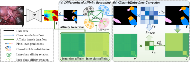
Figure 2: Illustration of Joint Class-Affinity Segmentation (JCAS) framework, including (a) differentiated affinity reasoning and (b) class-affinity loss correction.

The proposed Joint Class-Affinity Segmentation (JCAS) framework is illustrated in Fig. 2. Formally, we have access to training images $\mathcal{X}=\{\boldsymbol{X}\in\mathbb{R}^{H\times W\times 3}\}$ with spatial dimension of $H\times W$. The corresponding one-hot encoding of pixel-wise noisy labels is denoted as $\mathcal{Y}=\{\widetilde{\boldsymbol{Y}}\in\mathbb{R}^{H\times W\times C}\}$, where $C$ indicates the number of classes. We aim to learn a segmentation network that is robust to label noises in $\mathcal{Y}$ during the training process and could derive clean labels for test data. Given an input training image $\boldsymbol{X}$, a feature map $\boldsymbol{f}\in\mathbb{R}^{h\times w\times d}$ is first computed from the feature extractor $\mathcal{F}$. Note that $h$, $w$, and $d$ denote the height, width, and channel number of the feature map. Then, the feature map is passed through two branches for estimating pixel-wise predictions (upper branch in Fig. 2) and pair-wise affinity relations (lower branch in Fig. 2), respectively.

In the upper branch, a classifier $\mathcal{C}$ with softmax is used to produce the coarse segmentation result $\boldsymbol{Q}$. In the lower branch, an affinity generator is introduced to generate the affinity map $\boldsymbol{P^{\prime}}\in[0,1]^{n\times n}$ where $n$=$h\times w$, and the generator is formulated as $\boldsymbol{P^{\prime}}(k_{1},k_{2})=norm(\frac{\boldsymbol{f}(i_{1},j_{1})^{\top}\boldsymbol{f}(i_{2},j_{2})}{\left\|\boldsymbol{f}(i_{1},j_{1})\right\|_{2}\left\|\boldsymbol{f}(i_{1},j_{1})\right\|_{2}})$. $(i_{\cdot},j_{\cdot})$ is the coordinate of a pixel in feature map, and $(k_{1},k_{2})$ is the coordinate in affinity map. Note that $k_{1}$ and $(i_{1},j_{1})$ denote the position of the same pixel. The operator $norm(\cdot)$ performs normalization along each row to ensure affinity relations towards pixel $k_{1}$ are summed to 1, i.e., $\sum_{k_{2}}^{n}\boldsymbol{P^{\prime}}(k_{1},k_{2})=1$. The obtained affinity map $\boldsymbol{P^{\prime}}$ measures feature similarity between two pixels. Since intra-class pixels share the similar semantic features, intra-class pixel pairs usually show large similarity scores in $\boldsymbol{P^{\prime}}$, which highlights these pixel pairs belonging to the same class. Hence, $\boldsymbol{P^{\prime}}$ reveals the intra-class affinity relations. Then, we devise a differentiated affinity reasoning (DAR) module (Fig. 2 (a), Sec. 2.1) to obtain refined segmentation result $\boldsymbol{P}$, where the affinity map $\boldsymbol{P^{\prime}}$ derived in the lower branch is leveraged to guide the refinement of previously generated coarse segmentation result $\boldsymbol{Q}$ in the upper branch. Both pixel-wise segmentation prediction $\boldsymbol{P}$ and pair-wise affinity map $\boldsymbol{P^{\prime}}$ are regularized through the proposed class-affinity loss correction (CALC) strategy (Fig. 2 (b), Sec. 2.2). The optimized JCAS framework produces the refined segmentation result $\boldsymbol{P}$ as the final prediction in test phase.

2.1 Differentiated Affinity Reasoning (DAR)

In the image segmentation task, each image is equipped with a ground truth map, indicating pixel-wise semantic class label. Pixel-wise supervision signal cannot regularize the segmentation network to model the contextual dependencies from isolated pixels. Hence, we incorporate the contextual dependency embedded in the pair-wise affinity map $\boldsymbol{P^{\prime}}$ to guide the refinement of the pixel-wise segmentation result $\boldsymbol{Q}$. Moreover, different from existing affinity methods [18, 24] that aggregates contextual information as a mixture and may introduce undesirable contextual aggregations, we propose a differentiated affinity reasoning (DAR) module to explicitly distinguish intra-class and inter-class contextual dependencies and leverage the differentiated contexts to rectify segmentation predictions.

In addition to previously calculated pair-wise affinity map $\boldsymbol{P^{\prime}}$ that represents intra-class affinity relation, we infer the reverse affinity map $\boldsymbol{P^{\prime}_{re}}=norm(1-\boldsymbol{P^{\prime}})$. The reverse affinity map measures the dissimilarity between two pixels and reveals the inter-class affinity relations. The proposed DAR module performs intra-class and inter-class affinity reasonings, respectively. To be specific, the intra-class affinity reasoning aims to aggregate correlated information according to the intra-class affinity relations $\boldsymbol{P^{\prime}}$, and the inter-class affinity reasoning aims to eliminate irrelevant information according to the inter-class affinity relations $\boldsymbol{P^{\prime}}_{re}$, which can be formulated as:

$$\begin{split}\boldsymbol{P}_{intra}(k_{1})=\boldsymbol{P}(k_{1})+\sum_{k_{2}}^{n}\boldsymbol{P^{\prime}}(k_{1},k_{2})\boldsymbol{Q}(k_{2});\boldsymbol{P}_{inter}(k_{1})=\boldsymbol{P}(k_{1})-\sum_{k_{2}}^{n}\boldsymbol{P^{\prime}_{re}}(k_{1},k_{2})\boldsymbol{Q}(k_{2}).\end{split}$$ (1)

The refined pixel-wise prediction $\boldsymbol{P}$ is obtained through combining both intra-class and inter-class affinity reasoning results, i.e., $\boldsymbol{P}=\frac{1}{2}(\boldsymbol{P}_{intra}+\boldsymbol{P}_{inter})$. With the proposed DAR module, the correct predictions are strengthened, and the incorrect segmentation results are debiased and rectified.

2.2 Class-Affinity Loss Correction (CALC)

In multi-class image segmentation task, the widely used cross entropy loss is computed in a pixel-wise manner and formulated as $\mathcal{L}^{C}_{CE}=-\sum_{k}^{H\times W}\widetilde{\boldsymbol{Y}}(k)\log\boldsymbol{P}(k)$. However, directly minimizing the empirical risk of training data with respect to noisy labels $\widetilde{\boldsymbol{Y}}$ will lead to severely degraded generalizability. To reduce the noise rate, we introduce the pair-wise manner, and the corresponding affinity label is derived by $\boldsymbol{Y^{\prime}}(k1,k2)=\boldsymbol{Y}(k1)^{\top}\boldsymbol{Y}(k2)$. Only if two pixels share the same category, the value in the affinity label $\boldsymbol{Y^{\prime}}$ will be 1, otherwise $\boldsymbol{Y^{\prime}}$ will be 0. Although the pair-wise manner can greatly reduce the noise rate compared to the pixel-wise manner as demonstrated in Fig. 1, there still exist noises, and thus the binary entropy loss $\mathcal{L}^{A}_{Bi}=-\sum_{k}^{H\times W}\widetilde{\boldsymbol{Y}}(k)\log\boldsymbol{P^{\prime}}(k)+(1-\widetilde{\boldsymbol{Y}}(k))\log(1-\boldsymbol{P^{\prime}}(k))$ for affinity map supervision cannot guarantee the robustness of segmentation model towards label noises, resulting in biased semantic correlations. To facilitate the noise tolerance of $L^{C}_{CE}$ and $L^{A}_{Bi}$, we devise the class-affinity loss correction (CALC) strategy, including the class-level loss correction $\mathcal{L}^{C}_{LC}$ and affinity-level loss correction $\mathcal{L}^{A}_{LC}$. Meanwhile, a theoretically derived class-affinity consistency regularization $\mathcal{L}_{CACR}$ is advanced to unify pixel-wise and pair-wise supervisions.

Class-level Loss Correction. We model the label noise distributions in noisy class labels through a noise transition matrix (NTM) $\boldsymbol{T}_{C}\in[0,1]^{C\times C}$, which specifies the probability of clean label $m$ translating to noisy label $n$ via $\boldsymbol{T}_{C}(m,n)=p(\widetilde{Y}=n|Y=m)$. Hence, the probability of one pixel being predicted as $\widetilde{Y}=n$ is computed by $p(\widetilde{Y}=n)=\sum_{m=1}^{C}p(Y=m)\cdot\boldsymbol{T}_{C}(m,n)$, where $p(Y)$ is the clean class probability. Then the modeled noise label distribution is exploited to correct the supervision signal (i.e. $L^{C}_{CE}$) derived from noisy labels via $\mathcal{L}^{C}_{LC}=-\sum_{k}^{H\times W}\widetilde{\boldsymbol{Y}}(k)\log[\boldsymbol{P}(k)\boldsymbol{T}_{C}]$. This corrected loss encourages the consistency between noisy translated predictions and noisy class labels. Therefore, once the true NTM is obtained, the desired estimation of clean class predictions can be recovered by the output of segmentation model $\boldsymbol{P}$. For the estimation of the true NTM, we exploit the volume minimization regularization in [11].

Affinity-level Loss Correction. Similar to the class-level NTM, affinity-level NTM is defined as $\boldsymbol{T}_{A}\in[0,1]^{2\times 2}$, modeling the probability of clean affinity labels flipping to noisy affinity labels. Then, we exploit the modeled label noise distribution NTM to rectify the supervision signal (i.e. $L^{A}_{Bi}$) for affinity relation learning. Therefore, the affinity-level loss correction is formulated as $\mathcal{L}^{A}_{LC}=-\sum_{k}^{H\times W}\widetilde{\boldsymbol{Y}}(k)\log[\boldsymbol{P^{\prime}}(k)\boldsymbol{T}_{A}]+(1-\widetilde{\boldsymbol{Y}}(k))\log(1-\boldsymbol{P^{\prime}}(k)\boldsymbol{T}_{A})$.

Class-Affinity Consistency Regularization. To unify the pixel-wise and pair-wise supervisions, we bridge the class-level and affinity-level NTMs in Theorem 11. A theoretical proof for the Theorem is provided in Sec. 5 supplementary. Hence, the class-affinity consistency regularization is defined as $\mathcal{L}_{CACR}=\left\|\boldsymbol{T}_{C\to A}-\boldsymbol{T}_{A}\right\|_{2}$.

Combining the above defined losses, we obtain the joint loss of the proposed JCAS framwork as: $\mathcal{L}=\mathcal{L}^{C}_{LC}+\mathcal{L}^{A}_{LC}+\lambda\mathcal{L}_{CACR}$, which interacts the pixel-wise and pair-wise manners. Note that $\lambda$ is the weighting factor of $\mathcal{L}_{CACR}$.

Theorem 2.1

Assume that the class distribution of dataset denoting proportions of pixel number is $\mathcal{N}=[N_{1},N_{2},...,N_{C}]$, and the noise is class-dependent. Given a class-level NTM $\boldsymbol{T}_{C}$, the translated affinity-level NTM $\boldsymbol{T}_{C\to A}$ is calculated by

$$\footnotesize\begin{array}[]{l}\boldsymbol{T}_{C\to A}(0,0)=1-\boldsymbol{T}_{C\to A}(0,1),~{}\boldsymbol{T}_{C\to A}(0,1)=\frac{\sum_{m}\left[N_{m}\sum_{n}\boldsymbol{T}_{C}(m,n)\right]^{2}-\sum_{m}(N_{m})^{2}\left\|\boldsymbol{T}_{C}\right\|_{2}^{2}}{\sum_{m}\left[N_{m}(\sum_{m}N_{m}-N_{m})\right]},\\ \boldsymbol{T}_{C\to A}(1,0)=1-\boldsymbol{T}_{C\to A}(1,1),~{}\boldsymbol{T}_{C\to A}(1,1)=\frac{\sum_{m}(N_{m})^{2}\left\|\boldsymbol{T}_{C}\right\|_{2}^{2}}{\sum_{m}(N_{m})^{2}}.\end{array}$$ (2)

3 Experiments

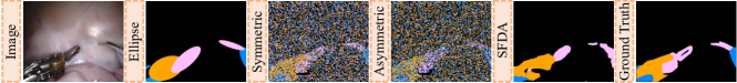
Figure 3: Illustration of dataset with different kinds of label noises.

Dataset. We validate the proposed JCAS method on the surgical instrument dataset Endovis18 [1]. It consists of 2384 images annotated with the instrument part labels, and the label space includes shaft, wrist and clasper classes, as shown in Fig. 3. The dataset is split into 1639 training images and 596 test images following [5]. Each image is resized into a resolution of 256$\times$320 in preprocessing.

Noise Patterns. To comprehensively verify the robustness of JCAS, we conduct experiments with both synthetic label noise (i.e., elipse, symmetric and asymmetric noises) and real-world label noise (i.e., noisy pseudo labels in source-free domain adaptation (SFDA)), as compared in Fig. 3. Specifically, the ellipse noisy label is a kind of weak annotation generated by drawing the minimal ellipse given the true segmentation label, greatly reducing the manual annotation cost. To simulate errors in the annotation process, ellipse labels are randomly dilated and eroded. Moreover, two commonly used label noises in the machine learning field, including symmetric and asymmetric noises with the rate of 0.5 [11, 23], are used to evaluate JCAS. Furthermore, we introduce Endovis17 [2] containing 1800 annotated images with domain shift to Endovis18, and generate realistic noisy labels from source only model trained on Endovis17.

Implementation. The proposed JCAS framework is implemented with PyTorch on Nvidia 2080Ti. DeepLabV2 [3] with the pre-trained encoder ResNet101 is our segmentation backbone. The initial learning rate is set as 1e-4 for the pre-trained encoder and 1e-3 for the rest of trainable parameters. We adopt a batch size of 3 and the maximum epoch number of 200. The weighting factor $\lambda$ is 0.01. The segmentation performance is assessed by $Dice$ and $Jac$ scores.

Table 1: Comparison under four label noises. Best and second best results are highlighted and underlined. ‘w/ Affinity’ introduces pair-wise supervision $\mathcal{L}^{A}_{Bi}$ to backbone.

Noises	Method	Shaft		Wrist		Clasper		Average
		Dice (%)	Jac (%)	Dice (%)	Jac (%)	Dice (%)	Jac (%)	Dice (%)	Jac (%)
	Upper bound	88.740	81.699	65.045	52.627	70.531	56.618	74.772	63.648
	RAUNet (19′) [13]	83.137	74.139	56.941	43.215	61.081	45.883	67.053	54.412
	LWANet (20′) [12]	81.945	72.735	53.626	40.886	64.364	49.781	66.645	54.468
Ellipse	CSS (21′) [14]	84.577	75.736	57.597	43.687	63.686	48.347	68.620	55.923
	MTCL (21′) [19]	72.719	60.540	39.386	27.474	49.662	35.085	53.922	41.033
	SR (21′) [23]	79.966	69.621	53.540	39.747	60.179	44.775	64.561	51.381
	VolMin (21′) [11]	81.320	70.758	60.470	46.408	58.203	42.524	66.664	53.230
	Baseline [3]	79.021	68.097	42.069	29.582	55.489	40.175	58.860	45.951
	w/ Affinity	82.158	72.339	49.128	35.455	58.933	43.594	63.406	50.463
	w/ DAR	82.698	72.992	52.207	38.442	61.544	46.027	65.483	52.487
	w/ CALC	82.973	73.126	61.885	47.527	60.416	44.821	68.425	55.158
	Ours (JCAS)	84.683	75.378	65.599	51.623	63.871	48.356	71.384	58.452
	RAUNet (19′) [13]	68.044	54.397	31.581	20.676	41.302	27.819	46.976	34.297
	LWANet (20′) [12]	0.294	0.150	10.089	5.908	10.228	5.489	6.870	3.849
Symmetric	CSS (21′) [14]	86.555	78.451	32.363	20.767	53.364	37.901	57.427	45.706
	MTCL (21′) [19]	78.480	67.855	50.011	38.013	55.515	40.411	61.336	48.760
	SR (21′) [23]	86.648	78.823	58.217	46.870	64.643	50.120	69.836	58.604
	VolMin (21′) [11]	86.811	78.834	63.712	51.259	66.604	52.096	72.376	60.730
	Baseline [3]	85.021	76.419	57.026	44.563	63.255	48.395	68.434	56.459
	Ours (JCAS)	88.285	80.692	65.759	53.487	68.129	53.821	74.058	62.667
	RAUNet (19′) [13]	87.255	79.983	59.462	46.639	67.347	52.801	71.355	59.808
	LWANet (20′) [12]	0.015	0.007	40.548	30.683	9.060	4.825	16.541	11.838
Asymmetric	CSS (21′) [14]	89.825	83.543	43.743	30.569	69.285	54.758	67.618	56.290
	MTCL (21′) [19]	74.544	62.525	41.433	30.533	48.077	33.676	54.685	42.244
	SR (21′) [23]	86.360	78.055	62.854	49.651	65.483	50.962	71.566	59.556
	VolMin (21′) [11]	86.840	78.796	63.345	51.137	65.220	50.996	71.802	60.310
	Baseline [3]	84.497	75.607	58.717	46.060	61.662	46.770	68.292	56.146
	Ours (JCAS)	88.247	80.730	67.298	54.922	67.686	53.436	74.410	63.029
	RAUNet (19′) [13]	73.370	61.568	56.063	42.570	45.979	31.720	58.471	45.286
	LWANet (20′) [12]	75.377	64.457	53.203	39.799	48.558	34.191	59.046	46.149
SFDA	CSS (21′) [14]	74.419	64.261	61.765	47.880	45.749	31.709	60.644	47.950
	MTCL (21′) [19]	72.289	60.346	51.095	37.972	38.762	25.567	54.048	41.295
	SR (21′) [23]	75.992	64.835	57.370	43.863	40.471	27.388	57.944	45.362
	VolMin (21′) [11]	76.641	65.063	58.285	44.389	41.780	28.324	58.902	45.925
	Baseline [3]	76.107	64.858	56.259	42.740	41.364	28.091	57.910	45.230
	Ours (JCAS)	76.540	65.300	59.904	46.104	48.725	34.283	61.723	48.562

Experiment results. Experimental comparison results under four types of label noises are presented in Table 1, in which we list the performance of upper bound (i.e., model trained with clean labels), three state-of-the-arts [13, 12, 14] in instrument segmentation, three label noise methods [19, 23, 11], our backbone [3], and the proposed JCAS. For a fair comparison, we reimplement [19, 23, 11] using the same backbone [3]. Compared with the aforementioned baselines, JCAS shows the minimum performance gap with the upper bound under all kinds of label noises, demonstrating the robustness of JCAS. Despite the satisfactory performance under ellipse and SFDA noises, LWANet [12] cannot deal with the other two types of noises, resulting in 6.870% and 16.541% $Dice$ scores. In contrast, JCAS shows comparable result to the upper bound with only 0.981% and 0.388% $Jac$ gaps under symmetric and asymmetric label noises. We further illustrate typical surgical instrument segmentation results in Fig. 4, validating the superiority of JCAS over baseline methods in the qualitative aspect.

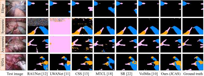
Figure 4: Comparison of segmentation results.

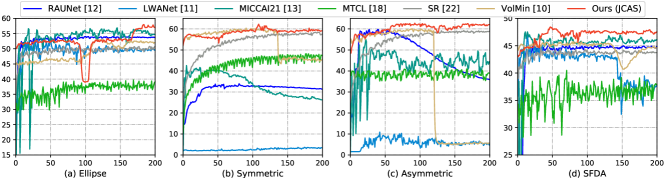
Figure 5: Curve of test $Jac$ vs. epoch with four different types of noise labels.

To analyze the influence of JCAS, we then conduct ablation study under ellipse noises. With the pair-wise manner (‘w/ Affinity’), the noise rate of supervision signals is greatly reduced, yielding an increment of 4.512% in $Jac$, while the increased memory overhead is negligible (from 780.71MB to 784.67MB). The devised DAR module (‘w/ DAR’) is also verified to be effective in differentiating contexture dependencies for the refinement of segmentation predictions, achieving an improvement of 9.207% $Jac$ score compared to the backbone. Moreover, the proposed CALC strategy further rectifies supervision signals derived from noisy labels and boosts the segmentation performance with 5.965% $Jac$ gain. To verify each component in DAR and CALC, we further ablate intra-class affinity reasoning ($1^{st}$ item in Eq. (1)), inter-class affinity reasoning ($2^{nd}$ item in Eq. (1)), $\mathcal{L}_{LC}^{C}$, $\mathcal{L}_{LC}^{A}$, and $\mathcal{L}_{CACR}$ under ellipse noises, obtaining 55.795%, 56.180%, 55.203%, 55.179%, 56.612% $Jac$. The performance of ablating each component is degraded compared to 58.452% $Jac$ achieved by our method (Table 1), verifying the effectiveness of individual component in mitigating label noise issue.

Furthermore, we show test $Jac$ curves in Fig. 5. While [11, 13] obtain promise results under ellipse and SFDA noises, they reach a high $Jac$ in the early stage and then decrease, overfitting to the other two noises. Notably, our JCAS converges to high performance under four noises and demonstrates more stable training process compared to [12, 14, 19], verifying its noise-resistant property.

4 Conclusion

In this paper, we propose a robust JCAS framework to combat label noise issues in medical image segmentation. Complementing the widely used pixel-wise manner, we introduce the pair-wise manner by capturing affinity relations among pixels to reduce noise rate. Then a DAR module is devised to rectify pixel-wise segmentation predictions by reasoning about intra-class and inter-class affinity relations. We further design a CALC strategy to unify pixel-wise and pair-wise supervisions, and facilitate noise tolerances of both supervisions. Extensive experiments under four noisy labels corroborate the noise immunity of JCAS.

5 Supplementary

5.1 Proof of Theorem 11

Theorem 5.1

Assume that the class distribution of dataset denoting proportions of pixel number is $\mathcal{N}=[N_{1},N_{2},...,N_{C}]$, and the noise is class-dependent. Given a class-level NTM $\boldsymbol{T}_{C}$, the translated affinity-level NTM $\boldsymbol{T}_{C\to A}$ is calculated by

$$\footnotesize\begin{array}[]{l}\boldsymbol{T}_{C\to A}(0,0)=1-\boldsymbol{T}_{C\to A}(0,1),~{}~{}\boldsymbol{T}_{C\to A}(0,1)=\frac{\sum_{m}\left[N_{m}\sum_{n}\boldsymbol{T}_{C}(m,n)\right]^{2}-\sum_{m}(N_{m})^{2}\left\|\boldsymbol{T}_{C}\right\|_{2}^{2}}{\sum_{m}\left[N_{m}(\sum_{m}N_{m}-N_{m})\right]},\\ \boldsymbol{T}_{C\to A}(1,0)=1-\boldsymbol{T}_{C\to A}(1,1),~{}~{}\boldsymbol{T}_{C\to A}(1,1)=\frac{\sum_{m}(N_{m})^{2}\left\|\boldsymbol{T}_{C}\right\|_{2}^{2}}{\sum_{m}(N_{m})^{2}}.\end{array}$$ (3)

Proof

Noise transition matrix (NTM) $\boldsymbol{T}_{C}\in[0,1]^{C\times C}$ specifies the probability of clean label $Y=m$ translating to noisy label $\widetilde{Y}=n$, which can be formulated as $\boldsymbol{T}_{C}(m,n)=p(\widetilde{Y}=n|Y=m)$. Taking the entry $\boldsymbol{T}_{C\to A}(0,0)$ of affinity-level NTM for example, we first calculate the number of pixel pairs with clean affinity labels $Y^{\prime}=0$ through $\sum_{m\neq m^{\prime}}N_{m}N_{m^{\prime}}\boldsymbol{T}_{C}(m,n)\boldsymbol{T}_{C}(m^{\prime},n^{\prime})$, and compute the number of data pairs with clean affinity labels $Y^{\prime}=0$ and noisy affinity labels $\widetilde{Y^{\prime}}=0$ via $\sum_{m\neq m^{\prime},n\neq n^{\prime}}N_{m}N_{m^{\prime}}\boldsymbol{T}_{C}(m,n)\boldsymbol{T}_{C}(m^{\prime},n^{\prime})$. Hence, the proportion of these two terms derives the element $\boldsymbol{T}_{C\to A}(0,0)=p(\widetilde{Y^{\prime}}=0|Y^{\prime}=0)=\frac{\sum_{m\neq m^{\prime},n\neq n^{\prime}}N_{m}N_{m^{\prime}}\boldsymbol{T}_{C}(m,n)\boldsymbol{T}_{C}(m^{\prime},n^{\prime})}{\sum_{m\neq m^{\prime}}N_{m}N_{m^{\prime}}\boldsymbol{T}_{C}(m,n)\boldsymbol{T}_{C}(m^{\prime},n^{\prime})}$. Similar to the derivation of entry $\boldsymbol{T}_{C\to A}(0,0)$, we can obtain the remaining three entries, and thus we have:

$$\boldsymbol{T}_{C\to A}(0,0)=\frac{\sum_{m\neq m^{\prime},n\neq n^{\prime}}N_{m}N_{m^{\prime}}\boldsymbol{T}_{C}(m,n)\boldsymbol{T}_{C}(m^{\prime},n^{\prime})}{\sum_{m\neq m^{\prime}}N_{m}N_{m^{\prime}}\boldsymbol{T}_{C}(m,n)\boldsymbol{T}_{C}(m^{\prime},n^{\prime})},$$ (4)

$$\boldsymbol{T}_{C\to A}(0,1)=\frac{\sum_{m\neq m^{\prime},n=n^{\prime}}N_{m}N_{m^{\prime}}\boldsymbol{T}_{C}(m,n)\boldsymbol{T}_{C}(m^{\prime},n^{\prime})}{\sum_{m\neq m^{\prime}}N_{m}N_{m^{\prime}}\boldsymbol{T}_{C}(m,n)\boldsymbol{T}_{C}(m^{\prime},n^{\prime})},$$ (5)

$$\boldsymbol{T}_{C\to A}(1,0)=\frac{\sum_{m=m^{\prime},n\neq n^{\prime}}N_{m}N_{m^{\prime}}\boldsymbol{T}_{C}(m,n)\boldsymbol{T}_{C}(m^{\prime},n^{\prime})}{\sum_{m=m^{\prime}}N_{m}N_{m^{\prime}}\boldsymbol{T}_{C}(m,n)\boldsymbol{T}_{C}(m^{\prime},n^{\prime})},$$ (6)

$$\boldsymbol{T}_{C\to A}(1,1)=\frac{\sum_{m=m^{\prime},n=n^{\prime}}N_{m}N_{m^{\prime}}\boldsymbol{T}_{C}(m,n)\boldsymbol{T}_{C}(m^{\prime},n^{\prime})}{\sum_{m=m^{\prime}}N_{m}N_{m^{\prime}}\boldsymbol{T}_{C}(m,n)\boldsymbol{T}_{C}(m^{\prime},n^{\prime})}.$$ (7)

Further, note that

$$\begin{split}\sum_{m\neq m^{\prime}}&N_{m}N_{m^{\prime}}\boldsymbol{T}_{C}(m,n)\boldsymbol{T}_{C}(m^{\prime},n^{\prime})\\ &=\sum_{m\neq m^{\prime}}(N_{m}\sum_{n}\boldsymbol{T}_{C}(m,n))(N_{m^{\prime}}\sum_{n^{\prime}}\boldsymbol{T}_{C}(m^{\prime},n^{\prime}))=\sum_{m\neq m^{\prime}}N_{m}N_{m^{\prime}}\\ &=\sum_{m}\left[N_{m}\sum_{m\neq m^{\prime}}N_{m^{\prime}}\right]=\sum_{m}\left[N_{m}(\sum_{m}N_{m}-N_{m})\right]\\ \end{split}$$ (8)

$$\begin{split}\sum_{m=m^{\prime}}&N_{m}N_{m^{\prime}}\boldsymbol{T}_{C}(m,n)\boldsymbol{T}_{C}(m^{\prime},n^{\prime})\\ &=\sum_{m=m^{\prime}}(N_{m}\sum_{n}\boldsymbol{T}_{C}(m,n))(N_{m^{\prime}}\sum_{n^{\prime}}\boldsymbol{T}_{C}(m^{\prime},n^{\prime}))=\sum_{m=m^{\prime}}N_{m}N_{m^{\prime}}\\ &=\sum_{m}(N_{m})^{2}\\ \end{split}$$ (9)

$$\begin{split}\sum_{m=m^{\prime},n=n^{\prime}}&N_{m}N_{m^{\prime}}\boldsymbol{T}_{C}(m,n)\boldsymbol{T}_{C}(m^{\prime},n^{\prime})\\ =&\sum_{m,n}\left[N_{m}\boldsymbol{T}_{C}(m,n)\right]^{2}=\sum_{m}(N_{m})^{2}\sum_{n}\left[\boldsymbol{T}_{C}(m,n)\right]^{2}=\sum_{m}(N_{m})^{2}\left\|\boldsymbol{T}_{C}\right\|_{2}^{2}\\ \end{split}$$ (10)

$$\begin{split}\sum_{m\neq m^{\prime},n=n^{\prime}}&N_{m}N_{m^{\prime}}\boldsymbol{T}_{C}(m,n)\boldsymbol{T}_{C}(m^{\prime},n)~{}~{}~{}~{}~{}~{}~{}~{}~{}~{}~{}~{}~{}~{}~{}~{}~{}~{}~{}~{}~{}~{}~{}~{}~{}~{}~{}~{}~{}~{}~{}~{}~{}~{}~{}~{}~{}~{}~{}~{}~{}~{}~{}~{}~{}\\ =&\sum_{m\neq m^{\prime}}(N_{m}\sum_{n}\boldsymbol{T}_{C}(m,n))(N_{m^{\prime}}\sum_{n}\boldsymbol{T}_{C}(m^{\prime},n))\\ =&\sum_{m}\left[N_{m}\sum_{n}\boldsymbol{T}_{C}(m,n)\right]^{2}-\sum_{m}(N_{m})^{2}\left\|\boldsymbol{T}_{C}\right\|_{2}^{2}\\ \end{split}$$ (11)

Substituting the derived equations above to Eq. (4-5), we have proved the Theorem .

5.2 Implementation of Class-Affinity Consistency Regularization

Given class-level noise transition matrix ($Tc$), affinity-level noise transition matrix ($Ta$), and class distribution ($N$), the proposed class-affinity consistency regularization can be derived through the code shown in Listing 1, and the completed code will be published online. Since the true class distribution is not available due to the noisy labels, we leverage the class distribution of pseudo labels generated from the warm-up model as an approximation.

⬇

1import torch

2

3def CACR_loss(Tc, Ta, N):

4 v00 = v01 = v10 = v11 = 0

5 num_classes = Tc.shape[0]

6 for m1 in range(num_classes):

7 for n1 in range(num_classes):

8 a = t[m1][n1]

9

10 for m2 in range(num_classes):

11 for n2 in range(num_classes):

12 b = t[m2][n2]

13

14 if m1 == m2 and n1 == n2:

15 v11 += a * b * N[m1] * N[m2]

16 if m1 == m2 and n1 != n2:

17 v10 += a * b * N[m1] * N[m2]

18 if m1 != m2 and n1 == n2:

19 v01 += a * b * N[m1] * N[m2]

20 if m1 != m2 and n1 != n2:

21 v00 += a * b * N[m1] * N[m2]

22

23 Tc_a = torch.zeros([2, 2]).cuda()

24 Tc_a[0][0] = v11 / (v11 + v10)

25 Tc_a[0][1] = v10 / (v11 + v10)

26 Tc_a[1][0] = v01 / (v01 + v00)

27 Tc_a[1][1] = v00 / (v01 + v00)

28 loss = torch.nn.MSELoss(reduction=’mean’)(Tc_a, Ta)

29 return loss

Listing 1: Implementation of class-affinity consistency regularization.

5.3 Visualization Results

We provide more surgical instrument segmentation results under four label noises, including ellipse (Fig. 6), symmetric (Fig. 7), asymmetric (Fig. 8) and SFDA (Fig. 9) noises. The qualitative comparison results demonstrate the superiority of the proposed JCAS framework in learning precise semantic correlations.

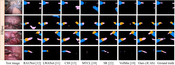
Figure 6: Illustration of dataset with ellipse label noises.

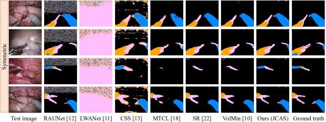
Figure 7: Illustration of dataset with symmetric label noises.

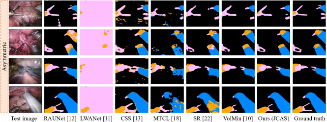
Figure 8: Illustration of dataset with asymmetric label noises.

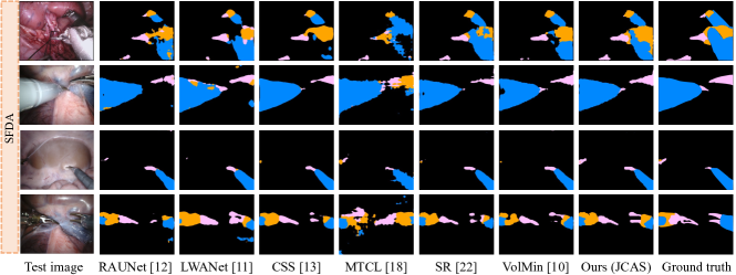
Figure 9: Illustration of dataset with SFDA label noises.

5.3.1 Acknowledgments.

This work was supported by Hong Kong Research Grants Council (RGC) Early Career Scheme grant 21207420 (CityU 9048179) and Hong Kong Research Grants Council (RGC) General Research Fund 11211221(CityU 9043152).

References

- [1] Allan, M., Kondo, S., Bodenstedt, S., Leger, S., Kadkhodamohammadi, R., Luengo, I., Fuentes, F., Flouty, E., Mohammed, A., Pedersen, M., et al.: 2018 robotic scene segmentation challenge. arXiv preprint arXiv:2001.11190 (2020)
- [2] Allan, M., Shvets, A., Kurmann, T., Zhang, Z., Duggal, R., Su, Y.H., Rieke, N., Laina, I., Kalavakonda, N., Bodenstedt, S., et al.: 2017 robotic instrument segmentation challenge. arXiv preprint arXiv:1902.06426 (2019)
- [3] Chen, L.C., Papandreou, G., Kokkinos, I., Murphy, K., Yuille, A.L.: Deeplab: Semantic image segmentation with deep convolutional nets, atrous convolution, and fully connected crfs. IEEE Trans. Pattern Anal. Mach. Intell. 40(4), 834–848 (2017)
- [4] Cheng, J., Liu, T., Ramamohanarao, K., Tao, D.: Learning with bounded instance and label-dependent label noise. In: ICML. pp. 1789–1799. PMLR (2020)
- [5] González, C., Bravo-Sánchez, L., Arbelaez, P.: Isinet: an instance-based approach for surgical instrument segmentation. In: MICCAI. pp. 595–605. Springer (2020)
- [6] Guo, X., Liu, J., Liu, T., Yuan, Y.: Simt: Handling open-set noise for domain adaptive semantic segmentation. In: CVPR (2022)
- [7] Guo, X., Yang, C., Li, B., Yuan, Y.: Metacorrection: Domain-aware meta loss correction for unsupervised domain adaptation in semantic segmentation. In: CVPR. pp. 3927–3936 (2021)
- [8] Karimi, D., Dou, H., Warfield, S.K., Gholipour, A.: Deep learning with noisy labels: Exploring techniques and remedies in medical image analysis. Med. Image Anal. 65, 101759 (2020)
- [9] Karimi, D., Vasylechko, S.D., Gholipour, A.: Convolution-free medical image segmentation using transformers. In: MICCAI. pp. 78–88. Springer (2021)
- [10] Li, S., Gao, Z., He, X.: Superpixel-guided iterative learning from noisy labels for medical image segmentation. In: MICCAI. pp. 525–535. Springer (2021)
- [11] Li, X., Liu, T., Han, B., Niu, G., Sugiyama, M.: Provably end-to-end label-noise learning without anchor points. In: ICML. pp. 6403–6413 (2021)
- [12] Ni, Z.L., Bian, G.B., Hou, Z.G., Zhou, X.H., Xie, X.L., Li, Z.: Attention-guided lightweight network for real-time segmentation of robotic surgical instruments. In: ICRA. pp. 9939–9945. IEEE (2020)
- [13] Ni, Z.L., Bian, G.B., Zhou, X.H., Hou, Z.G., Xie, X.L., Wang, C., Zhou, Y.J., Li, R.Q., Li, Z.: Raunet: Residual attention u-net for semantic segmentation of cataract surgical instruments. In: ICONIP. pp. 139–149. Springer (2019)
- [14] Pissas, T., Ravasio, C.S., Cruz, L.D., Bergeles, C.: Effective semantic segmentation in cataract surgery: What matters most? In: MICCAI. pp. 509–518. Springer (2021)
- [15] Shu, J., Xie, Q., Yi, L., Zhao, Q., Zhou, S., Xu, Z., Meng, D.: Meta-weight-net: Learning an explicit mapping for sample weighting. In: NeurIPS. pp. 1919–1930 (2019)
- [16] Wang, J., Zhou, S., Fang, C., Wang, L., Wang, J.: Meta corrupted pixels mining for medical image segmentation. In: MICCAI. pp. 335–345. Springer (2020)
- [17] Wu, S., Xia, X., Liu, T., Han, B., Gong, M., Wang, N., Liu, H., Niu, G.: Class2simi: A noise reduction perspective on learning with noisy labels. In: ICML. pp. 11285–11295 (2021)
- [18] Xu, L., Ouyang, W., Bennamoun, M., Boussaid, F., Sohel, F., Xu, D.: Leveraging auxiliary tasks with affinity learning for weakly supervised semantic segmentation. In: ICCV. pp. 6984–6993 (2021)
- [19] Xu, Z., Lu, D., Wang, Y., Luo, J., Jayender, J., Ma, K., Zheng, Y., Li, X.: Noisy labels are treasure: mean-teacher-assisted confident learning for hepatic vessel segmentation. In: MICCAI. pp. 3–13. Springer (2021)
- [20] Zhang, L., Tanno, R., Xu, M.C., Jin, C., Jacob, J., Cicarrelli, O., Barkhof, F., Alexander, D.: Disentangling human error from ground truth in segmentation of medical images. NeurIPS 33, 15750–15762 (2020)
- [21] Zhang, T., Yu, L., Hu, N., Lv, S., Gu, S.: Robust medical image segmentation from non-expert annotations with tri-network. In: MICCAI. pp. 249–258. Springer (2020)
- [22] Zhang, Z., Zhang, H., Arik, S.O., Lee, H., Pfister, T.: Distilling effective supervision from severe label noise. In: CVPR. pp. 9294–9303 (2020)
- [23] Zhou, X., Liu, X., Wang, C., Zhai, D., Jiang, J., Ji, X.: Learning with noisy labels via sparse regularization. In: ICCV. pp. 72–81 (2021)
- [24] Zhu, X., Chen, J., Zeng, X., Liang, J., Li, C., Liu, S., Behpour, S., Xu, M.: Weakly supervised 3d semantic segmentation using cross-image consensus and inter-voxel affinity relations. In: ICCV. pp. 2834–2844 (2021)