Personalized Federated Learning via Variational Bayesian Inference

Abstract

Federated learning faces huge challenges from model overfitting due to the lack of data and statistical diversity among clients. To address these challenges, this paper proposes a novel personalized federated learning method via Bayesian variational inference named pFedBayes. To alleviate the overfitting, weight uncertainty is introduced to neural networks for clients and the server. To achieve personalization, each client updates its local distribution parameters by balancing its construction error over private data and its KL divergence with global distribution from the server. Theoretical analysis gives an upper bound of averaged generalization error and illustrates that the convergence rate of the generalization error is minimax optimal up to a logarithmic factor. Experiments show that the proposed method outperforms other advanced personalized methods on personalized models, e.g., pFedBayes respectively outperforms other SOTA algorithms by 1.25%, 0.42% and 11.71% on MNIST, FMNIST and CIFAR-10 under non-i.i.d. limited data.

1 Introduction

Federated learning (FL) is an increasingly popular topic in deep learning, which can model machine learning for distributed end devices while preserving their privacy (McMahan et al., 2017; Li et al., 2020). With the increasing emphasis on privacy protection, federated learning has been widely used in finance, medicine, internet of things, internet of vehicles and e-commerce. When data from different clients are assumed to be independent and identically distributed (i.i.d.), federated learning performs well and has a strict convergence guarantee. However, there are two main challenges caused by imperfect data, one is that private data from different clients are usually non-i.i.d. due to the differences in user preferences, locations, and living habits, leading to model performance degradation; the other is that data from clients are usually limited and not enough to train a large neural network with too many parameters, leading to model overfitting. A natural question is can we design a federated learning algorithm to address these two challenges caused by data together?

To overcome this challenge caused by non-i.i.d. data, personalized federated learning (PFL) (Li et al., 2018; T Dinh et al., 2020; Huang et al., 2021) is proposed to achieve personalization. Although standard PFL has come a long way in non-i.i.d. data, model overfitting often occurs when data from the client is limited. Recently, the Bayesian neural network (BNN) is introduced into FL to address the model overfitting by representing all network parameters in the global model with probability distributions (Chen & Chao, 2021; Thorgeirsson & Gauterin, 2021). Unfortunately, these algorithms show performance degradation when data from different clients have statistical diversity. Our goal is to find a way to address the challenges from non-i.i.d. data and limited data simultaneously.

In this paper, we find an efficient way to adapt BNN into PFL and propose a novel PFL model through variational Bayesian inference. Unlike traditional BNNs, we do not assume a prior distribution for each parameter on the end devices; instead, the trained global distribution is used as the prior distribution. It is well known that the assumed prior distribution often does not match the true distribution. Our model can avoid this flaw by using a trained global distribution. Furthermore, the proposed model can quantify the uncertainty of the network output by using Bayesian model averaging, which has practical implications in various robustness-critical applications such as medical diagnosis, autonomous driving, and financial transactions (Jospin et al., 2020).

1.1 Main Contributions

This paper proposes a novel two-level personalized federated learning model named pFedBayes based on variational Bayesian inference. Both local and global neural networks are formulated as BNN, where all network parameters are treated as random variables. The server seeks to minimize the KL divergence between the global distribution and all local distributions. The local model encourages clients to find a local distribution that balances the construction error over its private data and the KL divergence with global distribution. It should be stressed that pFedBayes not only achieves personalization under limited data conditions, but also quantifies the output uncertainty, which can meet the requirements of many practical applications.

Next, we provide the theoretical guarantee for the proposed model pFedBayes. We give the upper bound on the averaged generalization error across all clients, which shows that the upper bound consists of estimation error and approximation error and the estimation error is on the order of $1/n$. Furthermore, by choosing a suitable number of network parameters, we prove that the averaged generalization error achieves minimax optimal convergence rate up to a logarithmic term.

Finally, we propose a computationally efficient algorithm by using the one-order stochastic gradient algorithm for clients and the server alternatively and compare the performance of pFedBayes with other state-of-the-art (SOTA) algorithms under statistical diversity conditions. Various experimental results present that the proposed algorithm has a better performance than other SOTA personalization algorithms, especially in the case of limited data. In particular, pFedBayes has the highest accuracy on personalized models on MNIST, FMNIST and CIFAR-10 datasets with small, medium, and large data volumes, and pFedBayes has competitive performance on the global models when the amount of data is small and medium.

1.2 Related Works

Personalized Bayesian federated learning is closely related to the following topics:

Federated learning. Google group proposed the first federated learning algorithm named FedAvg (Federated Averaging) to protect the privacy of clients in distributed learning (McMahan et al., 2017). Many variants of FedAvg were proposed to meet different demands from various scenarios. To reduce the round of communication, communication-efficient algorithms were considered in federated learning such as approximate Newton’s algorithm (Li et al., 2019), primal-dual algorithm (Zhang et al., 2020) and one-shot averaging algorithm (Guha et al., 2019). To reduce the data size of storage and communication, sparsity (Sattler et al., 2019; Rothchild et al., 2020) and quantization (Dai et al., 2019; Reisizadeh et al., 2020; Zong et al., 2021) were studied in federated learning. These algorithms focus on learning a global model for all clients, which presents poor performance when private data from different clients are non-i.i.d.

Personalized federated learning. To address the challenge from heterogeneous datasets, researchers proposed a number of PFL methods including local customization methods (Li et al., 2018; Arivazhagan et al., 2019; Hanzely & Richtárik, 2020; T Dinh et al., 2020; Huang et al., 2021; Li et al., 2021; Liu et al., 2022), multi-task learning based methods (Smith et al., 2017; Sattler et al., 2021), meta-learning based methods (Chen et al., 2018; Fallah et al., 2020) and others (Li et al., 2022a, b). Local customization methods customize a personalized model for each client. For example, Li et al. (2018) proposed a variant of FedAvg named Fedprox by adding a proximal term in the subproblems; Huang et al. (2021) proposed FedAMP and HeurFedAMP by designing an attentive message passing mechanism to facilitate more collaborations of similar clients. Two-level modeling is a special kind of customization method, which is composed of the sever-level subproblem and client-level subproblems. In particular, pFedMe (T Dinh et al., 2020) penalized the $\ell_{2}$ norm of the difference between the local parameter and global parameter in the client-level subproblem, which has a similar two-level optimization problem with pFedBayes but has a poor performance for small datasets. For the multi-task learning based method, Smith et al. (2017) first introduced multi-task learning into federated learning and proposed a robust optimization method. Then Sattler et al. (2021) proposed a clustered federated learning to realize personalization by using the geometric properties of the loss function. Regrading the meta-learning based methods, Fallah et al. (2020) considered a variant of FedAvg named per-FedAvg by jointly obtaining an initial model and then applying it to each client. Although these advanced algorithms improve the performance on non-i.i.d. data, they suffer from overfitting when the amount of data is limited.

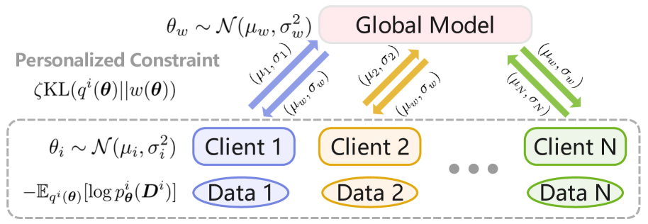
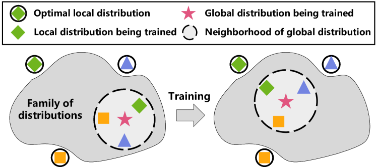
Figure 1: Personalized Bayesian federated learning model under Gaussian assumptions. Left: System diagram. Each client uploads its updated distribution to the server and then downloads the aggregated global distribution from the server. Right: Distribution Training. The subfigure shows the evolution of training the local and global distributions in probability space.

Bayesian neural network and Bayesian federated learning. To overcome the overfitting caused by limited data, the Bayesian neural network (MacKay, 1992; Neal, 2012; Blundell et al., 2015b) was proposed by imposing a prior distribution on each parameter (weights and biases). The authors in (Pati et al., 2018; Chérief-Abdellatif & Alquier, 2018; Maddox et al., 2019; Alquier & Ridgway, 2020; Bai et al., 2020; Chérief-Abdellatif, 2020) studied the generalization error bounds and gave the concentration of variational approximation for different statistical models. To alleviate the overfitting in FL, a Bayesian ensemble was introduced into FL. Yurochkin et al. (2019) proposed a Bayesian nonparametric federated learning (BNFed) framework by neural parameter matching based on the Beta-Bernoulli process. Chen & Chao (2021) proposed FedBE by applying the Bayesian model to the global model and treating local distributions as Gaussian or Dirichlet distributions. Based on FedAvg, Thorgeirsson & Gauterin (2021) introduced Gaussian distribution to each parameter and aggregated the local models by calculating the mean and variance of uploaded parameters. However, the above models have poor performance when data are non-i.i.d. Al-Shedivat et al. (2021) proposed an approximate posterior inference algorithm named FedPA by inferring global posterior via the average of local posteriors, but FedPA is inapplicable for PFL. Achituve et al. (2021) proposed a personalized model based on Gaussian processes named pFedGP, which learns a shared deep kernel function for all clients and a personalized Gaussian process classifier using a personal dataset for each client. Since all the clients use a common kernel function, the performance might degrade when data varies widely. Different from pFedGP, each client in our model owns its personalized BNN, which is more flexible and robust in practical applications. Liu et al. (2021) proposed an FL model named FOLA to achieve personalization, where Gaussian approximate posterior distribution of the server parameter is considered as the client’s prior. But FOLA is based on Maximum a posteriori estimation while the pFedBayes is based on a Bayesian two-level optimization. Furthermore, FOLA lacks theoretical analysis, but pFedBayes has theoretical guarantees.

2 Personalized Bayesian Federated Learning Model with Gaussian Distribution

In this section, we present the personalized Bayesian federated learning model with Gaussian distribution. In our model, each client owns its BNN, where each parameter (weight or bias) denotes a Gaussian distribution. Compared with the classical neural network, we only use twice the number of parameters to construct a BNN, but includes an infinite number of classical neural network. As shown in Fig. 1(a), at each iteration, the clients upload their distributions (i.e., mean and variance) to the server and then download the aggregated distribution from the server. In Fig. 1(b), we show the evolution of the distribution training, where the global model (GM) serves as the prior of the personalized models (PMs). The figure presents that the trained distribution for each PM lies between the GM and PM without communication, which balances the GM and extreme PM without communication.

Next, we show the proposed model explicitly. Considering a distributed system that contains one server and $N$ clients. For ease of analysis, we assume the variance of noise for all clients is the same and the number of data is the same. Let the $i$-th client satisfy the model

$$\bm{y}_{j}^{i}=f^{i}(\bm{x}_{j}^{i})+\varepsilon_{j}^{i},\,j=1,\ldots,n,\,\varepsilon_{j}^{i}\sim\mathcal{N}(0,\sigma_{\varepsilon}^{2}),$$ (1)

where $\bm{x}_{j}^{i}\in\mathbb{R}^{s_{0}}$, $\bm{y}_{j}^{i}\in\mathbb{R}^{s_{L+1}}$ for $j=1,\ldots,n$, $i=1,\ldots,N$, $f^{i}(\cdot):\mathbb{R}^{s_{0}}\to\mathbb{R}^{s_{L+1}}$ denotes a nonlinear function, $n$ denotes the sample size and $\sigma_{\varepsilon}$ denotes the variance of noise. Define the dataset for $i$-th client as $\bm{D}^{i}=(\bm{D}_{1}^{i},\ldots,\bm{D}_{n}^{i})$, where $\bm{D}_{j}^{i}=(\bm{x}_{j}^{i},\bm{y}_{j}^{i})$. Let $P^{i}$ denote the probability measure of data for the $i$-th client and $p^{i}$ be its corresponding probability density function.

Suppose each client has the same neural network architecture, i.e., a fully-connected Deep Neural Network (DNN), but has different parameters due to the fact that their data are non-i.i.d. In particular, the neural network has $L$ hidden layers, where the $j$-th hidden layer has $s_{j}$ neurons and activation functions $\sigma(\cdot),j=1,\ldots,L$. The output of the DNN model is represented as $f_{\bm{\theta}}(\bm{x})$, where $\bm{\theta}\in\mathbb{R}^{T}$ denotes the vector that contains all parameters and $T$ is the length of $\bm{\theta}$. Define $\bm{s}=\{s_{1},\ldots,s_{L}\}$. Assume that all parameters are bounded, i.e., there exixts some constant $B>0$ such that $\left\lVert\bm{\theta}\right\rVert_{\infty}\leq B$. Then we denote the DNN model for the $i$-th client as $f_{\bm{\theta}}^{i}$.

Our goal is to design an FL model that achieves personalization and alleviates overfitting simultaneously. Before giving a personalized Bayesian FL model, we first review the standard BNN model via variational inference (Jordan et al., 1999; Blei et al., 2017). The optimization problem aims to find the closest distribution to the posterior distribution in the variational family of distributions $\mathcal{Q}$

$$\min_{q(\bm{\theta})\in\mathcal{Q}}\mbox{KL}(q(\bm{\theta})||\pi(\bm{\theta}|\bm{D})),$$ (2)

where $\pi(\bm{\theta}|\bm{D})$ denotes the posterior distribution and $\bm{D}$ denotes the collected data. Using Bayes theorem gives $\pi(\bm{\theta}|\bm{D})\propto\pi(\bm{\theta})p_{\bm{\theta}}(\bm{D})$, where $\pi(\bm{\theta})$ denotes the prior distribution and $p_{\bm{\theta}}(\bm{D})$ denotes the likelihood. So the above optimization problem is equivalent to the following problem

$$\min_{q(\bm{\theta})\in\mathcal{Q}}-\mathbb{E}_{q(\bm{\theta})}[\log p_{\bm{\theta}}(\bm{D})]+\mbox{KL}(q(\bm{\theta})||\pi(\bm{\theta})),$$ (3)

where the first term can be regarded as the reconstruction error on the dataset $\bm{D}$ and the second term is a regularization with the prior distribution.

Based on the standard BNN model, we propose a novel personalized federated learning model via variational Bayesian inference named pFedBayes, which is formulated as the following two-level optimization problem

Server: $$~{}\min_{w(\bm{\theta})\in\mathcal{Q}_{w}}\left\{F(w)\triangleq\frac{1}{N}\sum_{i=1}^{N}F_{i}(w)\right\},$$ (4)

$$\text{Clients:}~{}F_{i}(w)\triangleq\min_{q^{i}(\bm{\theta})\in\mathcal{Q}^{i}}\Big{\{} -\mathbb{E}_{q^{i}(\bm{\theta})}[\log p^{i}_{\bm{\theta}}(\bm{D}^{i})]$$

$$+\zeta\,\mbox{KL}(q^{i}(\bm{\theta})||w(\bm{\theta}))\Big{\}}.$$ (5)

where $w(\bm{\theta})$ and $q^{i}(\bm{\theta})$ denote the global distribution and the local distribution for the $i$-th client to be optimized, respectively, $\mathcal{Q}_{w}$ and $\mathcal{Q}^{i}$ denote the family of distributions for global parameter and the $i$-th client, respectively, and $p^{i}_{\bm{\theta}}(\bm{D}^{i})$ denotes the likelihood for the $i$-th client. By minimizing the sum of KL divergence, the global model can find the closest distribution in $Q_{w}$ to the clients’ distribution. Note that in the regularization term for clients, we replace prior distribution with global distribution. The reason is that since we cannot characterize the prior distribution in practice, it’s difficult to assume a good prior distribution that is compatible with the collected data. Instead, by replacing the prior distribution with trained global distribution, we find a relatively good distribution without making assumptions about the prior distribution. Motivated by the modification in $\beta$-VAE (Higgins et al., 2017), there is an extra parameter $\zeta\geq 1$ in the subproblem that balances the degree of personalization and global aggregation.

In this paper, we assume that the parameters of the neural network follow Gaussian distribution, which is commonly used in the literature (Blundell et al., 2015a; Chen & Chao, 2021; Thorgeirsson & Gauterin, 2021). Besides, it’s common to assume that the distribution satisfies mean-field decomposition, that is, the joint distribution equals to the product of each parameter’s distribution. In particular, assume that the family of distributions of the $i$-th client $\mathcal{Q}^{i}$ satisfies

$$\theta_{i,m}\sim\mathcal{N}(\mu_{i,m},\sigma^{2}_{i,m}),~{}m=1,\ldots,T,$$ (6)

where $\mu_{i,m}$ denotes the Gaussian mean and $\sigma^{2}_{i,m}$ denotes the Gaussian variance for $m$-th parameter of the $i$-th client. Let the family of distributions of the server $\mathcal{Q}_{w}$ follow

$$\theta_{w,m}\sim\mathcal{N}(\mu_{w,m},\sigma^{2}_{w,m}),~{}m=1,\ldots,T,$$ (7)

where $\mu_{w,m}$ denotes the Gaussian mean and $\sigma^{2}_{w,m}$ denotes the Gaussian variance for $m$-th parameter of the server.

Armed with the above distributions, we can obtain the KL divergences of the two Gaussian distributions $q^{i}(\bm{\theta})$ and $w(\bm{\theta})$ as follows

$$~{}\mbox{KL}(q^{i}(\bm{\theta})||w(\bm{\theta}))$$

$$= ~{}\mbox{KL}\left(\prod^{T}_{m=1}\mathcal{N}(\mu_{i,m},\sigma^{2}_{i,m})\Bigl{|}\Bigr{|}\prod^{T}_{m=1}\mathcal{N}(\mu_{w,m},\sigma^{2}_{w,m})\right)$$

$$= ~{}\sum_{m=1}^{T}\mbox{KL}(\mathcal{N}(\mu_{i,m},\sigma^{2}_{i,m})||\mathcal{N}(\mu_{w,m},\sigma^{2}_{w,m}))$$ (8)

$$= ~{}\frac{1}{2}\sum_{m=1}^{T}\left[\log\left(\frac{\sigma_{w,m}^{2}}{\sigma_{i,m}^{2}}\right)+\frac{\sigma_{i,m}^{2}+(\mu_{i,m}-\mu_{w,m})^{2}}{\sigma_{w,m}^{2}}-1\right].$$

3 Theoretical Analysis

In this section, we will provide theoretical analysis for averaged generalization error of the proposed model and show the minimax optimality of the convergence rate of the generalization error. The proofs of the main results are put in the Appendices.

Before that, we give some necessary assumptions. For simplicity, we analyse the equal-width Bayesian neural network as Polson & Ročková (2018) and Bai et al. (2020). And we study a general activation function that satisfies $1$-Lipschitz continuous.

Assumption 1.

The widths of neural network are equal-width, i.e., $s_{i}=M.$

Assumption 2.

The activation function $\sigma(\cdot)$ is $1$-Lipschitz continuous.

Assumption 3.

The parameters $s_{0},n,M,L$ are large enough such that

$$\sigma^{2}_{n}=\frac{T}{8n}A\leq B^{2},$$ (9)

where $H=BM$ and

$$A=\log^{-1}(3s_{0}M)\cdot(2H)^{-2(L+1)}$$

$$\left[\left(s_{0}+1+\frac{1}{H-1}\right)^{2}+\frac{1}{(2H)^{2}-1}+\frac{2}{(2H-1)^{2}}\right]^{-1}.$$ (10)

Remark 1.

This sequence ${\sigma_{n}^{2}}$ is constructed to prove Lemma 2. Since the neural parameters are bounded by $B$, their variance should be upper bounded by $B^{2}$. The above assumption is easy to be satisfied due to the fact that $A/8n$ can be arbitrarily small.

Next, we give some useful definitions. Define the Hellinger distance as follows

$$d^{2}(P_{\bm{\theta}}^{i},P^{i})=\mathbb{E}_{X^{i}}\Bigl{(}1-\exp\{-[f_{\bm{\theta}}^{i}(X^{i})-f^{i}(X^{i})]^{2}/(8\sigma^{2}_{\epsilon})\}\Bigr{)}.$$

Define the following terms

$$r_{n} =((L+1)T/n)\log M+(T/n)\log(s_{0}\sqrt{n/T}),$$ (11)

$$\xi^{i}_{n} =\inf_{\bm{\theta}\in{\Theta}(L,\bm{s}),\|\bm{\theta}\|_{\infty}\leq B}||f_{\bm{\theta}}^{i}-f^{i}||^{2}_{\infty},$$ (12)

$$\varepsilon_{n} =n^{-\frac{1}{2}}\sqrt{(L+1)T\log M+T\log(s_{0}\sqrt{n/T})}\log^{\delta}(n),$$ (13)

where $\delta>1$.

Since the incorporation of a constant that is unrelated to $\bm{\theta}$ doesn’t affect the optimization problem, we rewrite the subproblem for clients as follows

$$\text{Clients:}~{}F_{i}(w)\triangleq\min_{q^{i}(\bm{\theta})\in\mathcal{Q}^{i}} \Big{\{}\int_{\Theta}l_{n}(P^{i},P^{i}_{\bm{\theta}})q^{i}(\bm{\theta})d\bm{\theta}$$

$$+\zeta\,\mbox{KL}(q^{i}(\bm{\theta})||w(\bm{\theta}))\Big{\}},$$ (14)

where $l_{n}(P^{i},P^{i}_{\bm{\theta}})$ is the log-likelihood ratio of $P^{i}$ and $P^{i}_{\bm{\theta}}$

$$l_{n}(P^{i},P^{i}_{\bm{\theta}})=\log\frac{p^{i}(\bm{D}^{i})}{p^{i}_{\bm{\theta}}(\bm{D}^{i})}.$$ (15)

Let $w^{\star}(\bm{\theta})$ be the optimal variational solution of the problem and $\hat{q}^{i}(\bm{\theta})$ be its corresponding variational solution for the $i$-th client’s subproblem

$$\hat{q}^{i}(\bm{\theta})=\arg\inf_{q^{i}(\bm{\theta})\in\mathcal{Q}^{i}}\Big{\{} \int_{\Theta}l_{n}(P^{i},P^{i}_{\bm{\theta}})q^{i}(\bm{\theta})d\bm{\theta}$$

$$+\zeta\,\mbox{KL}(q^{i}(\bm{\theta})||w^{\star}(\bm{\theta}))\Big{\}}.$$ (16)

Our purpose is to give an upper bound for the term

$$\frac{1}{N}\sum_{i=1}^{N}\int_{\Theta}d^{2}(P_{\bm{\theta}}^{i},P^{i})\hat{q}^{i}(\bm{\theta})d\bm{\theta}.$$ (17)

with parameters $r_{n}$, $\xi^{i}_{n}$ and $\varepsilon_{n}$.

We first bound Eq. (17) by the average of objective functions of all subproblems as follows.

Lemma 1.

Suppose that the assumptions 1 and 2 are true, then with dominating probability, the following inequality holds

$$\frac{1}{N} \sum_{i=1}^{N}\int_{\Theta}d^{2}(P_{\bm{\theta}}^{i},P^{i})\hat{q}^{i}(\bm{\theta})d\bm{\theta}\leq$$

$$\frac{1}{n}\Bigg{\{}\frac{1}{N}\sum_{i=1}^{N}\Bigg{[}\frac{1}{\zeta}\int_{\Theta}l_{n}(P^{i},P^{i}_{\bm{\theta}})\hat{q}^{i}(\bm{\theta})d\bm{\theta}$$

$$\qquad\qquad\quad+\mbox{\rm KL}(\hat{q}^{i}(\bm{\theta})||w^{\star}(\bm{\theta}))\Bigg{]}\Bigg{\}}+C\varepsilon^{2}_{n},$$ (18)

where $\zeta\geq 1$ is a tradeoff parameter and $C>0$ is an absolute constant.

Then we present the upper bound of the average of objective functions for $N$ subproblems.

Lemma 2.

Suppose that the assumptions are true, then with dominating probability, the following inequality holds

$$\frac{1}{N}\sum_{i=1}^{N}\left[\int_{\Theta}l_{n}(P^{i},P^{i}_{\bm{\theta}})\hat{q}^{i}(\bm{\theta})d\bm{\theta}+\zeta\,\mbox{\rm KL}(\hat{q}^{i}(\bm{\theta})||w^{\star}(\bm{\theta}))\right]\\ \leq n\left(C^{\prime}\zeta r_{n}+\frac{C^{\prime\prime}}{N}\sum_{i=1}^{N}\xi^{i}_{n}\right),$$ (19)

where $\zeta\geq 1$ is a tradeoff parameter and $C^{\prime},C^{\prime\prime}$ are any diverging sequences.

Combining Lemmas 1 and 2 yields the main theorem.

Theorem 1.

Suppose that the assumptions are true, then the following upper bound holds with dominating probability

$$\frac{1}{N}\sum_{i=1}^{N}\int_{\Theta}d^{2}(P_{\bm{\theta}}^{i},P^{i})\hat{q}^{i}(\bm{\theta})d\bm{\theta}\\ \leq C\varepsilon^{2}_{n}+C^{\prime}r_{n}+\frac{C^{\prime\prime}}{N\zeta}\sum_{i=1}^{N}\xi^{i}_{n},$$ (20)

where $\zeta\geq 1$ is a tradeoff parameter, $C>0$ is an absolute constants and $C^{\prime},C^{\prime\prime}$ are any diverging sequences.

The upper bound can be divided into two parts: the first and second terms belong to the estimation error while the third term is the approximation error. Note that the estimation error decreases with the increase of sample size $n$. For the approximation error, it is only related to the total number of parameters $T$ (or the width and depth) of the neural network. Besides, with the increase of $T$, the estimation error increases but the approximation error decreases. Therefore, a suitable parameter $T$ should be chosen as a function of sample size $n$ to balance the upper bound.

Next, we present the choice of $T$ for a typical class of functions. Assume that $\{f^{i}\}$ are $\beta$-Hölder-smooth functions and the intrinsic dimension of data is $d$. According to Corollary 6 in (Nakada & Imaizumi, 2020), the approximation error is bounded as follows

$$\xi^{i}_{n}\leq C_{0}T^{-2\beta/d},i=1,\ldots,N,$$ (21)

where $C_{0}>0$ is a constant related to $s_{0}$, $\beta$ and $d$. By using Theorem 1 and choosing $T=C_{1}n^{d/(2\beta+d)}$, we can give the convergence rate of the upper bound

$$\frac{1}{N}\sum_{i=1}^{N}\int_{\Theta}d^{2}(P_{\bm{\theta}}^{i},P^{i})\hat{q}^{i}(\bm{\theta})d\bm{\theta}\leq C_{2}n^{-\frac{2\beta}{2\beta+d}}\log^{2\delta^{\prime}}(n),$$ (22)

where $\delta^{\prime}>\delta>1$, and $C_{1},C_{2}>0$ are constants related to $s_{0}$, $\beta$, $d$, $L$, $M$, $\zeta$ and $n$.

Finally, we show the minimax optimality of the generalization error rate. Similar to Theorem 1.1 from (Bai et al., 2020), we can represent the convergence result under $L^{2}$ norm. By using the monotonically decreasing property of $[1-\exp(-x^{2})]/{x^{2}}$ when $x>0$, for bounded functions $\left\lVert f^{i}\right\rVert_{\infty}\leq F$ and $\left\lVert f_{\bm{\theta}}^{i}\right\rVert_{\infty}\leq F$, $i=1,\ldots,N$, we have

$$\frac{d^{2}(P_{\bm{\theta}}^{i},P^{i})}{\left\lVert f_{\bm{\theta}}^{i}(X^{i})-f^{i}(X^{i})\right\rVert_{L^{2}}^{2}}\geq\frac{1-\exp(-\frac{4F^{2}}{8\sigma_{\epsilon}^{2}})}{4F^{2}}\triangleq C_{F}.$$ (23)

Then we can give an upper bound under $L^{2}$ norm like (22)

$$\frac{C_{F}}{N}\sum_{i=1}^{N}\int_{\Theta}\left\lVert f_{\bm{\theta}}^{i}(X^{i})-f^{i}(X^{i})\right\rVert_{L^{2}}^{2}\hat{q}^{i}(\bm{\theta})d\bm{\theta}\\ \leq\frac{1}{N}\sum_{i=1}^{N}\int_{\Theta}d^{2}(P_{\bm{\theta}}^{i},P^{i})\hat{q}^{i}(\bm{\theta})d\bm{\theta}\\ \leq C_{2}n^{-\frac{2\beta}{2\beta+d}}\log^{2\delta^{\prime}}(n).$$ (24)

According to the minimax lower bound under $L^{2}$ norm in Theorem 8 of (Nakada & Imaizumi, 2020), we obtain

$$\inf_{\{\left\lVert f_{\bm{\theta}}^{i}\right\rVert\leq F\}_{i=1}^{N}}\sup_{\{\left\lVert f^{i}\right\rVert_{\infty}\leq F\}_{i=1}^{N}}\frac{C_{F}}{N}\sum_{i=1}^{N}\\ \int_{\Theta}\left\lVert f_{\bm{\theta}}^{i}(X^{i})-f^{i}(X^{i})\right\rVert_{L^{2}}^{2}\hat{q}^{i}(\bm{\theta})d\bm{\theta}\geq C_{3}n^{-\frac{2\beta}{2\beta+d}},$$ (25)

where $C_{3}>0$ is a constant.

Combining Eqs. (24) and (25), we conclude that the convergence rate of the generalization error of pFedBayes is minimax optimal up to a logarithmic term for bounded functions $\{f^{i}\}_{i=1}^{N}$ and $\{f^{i}_{\bm{\theta}}\}_{i=1}^{N}$.

Remark 2.

According to Theorem 1, we notice that with the increase of $\zeta$, the approximation error in the upper bound decreases, so does the upper bound. But from the formulation of the proposed optimization problem, we know the increase of $\zeta$ will decrease the degree of personalization. So a suitable choice of $\zeta$ is necessary to balance the degree of personalization and the value of the global upper bound.

Algorithm 1 pFedBayes: Personalized Federated Learning via Bayesian Inference Algorithm

Cloud server executes:

Input $T,R,S,\lambda,\eta,\beta,b,\bm{v}^{0}=(\bm{\mu}^{0},\bm{\sigma}^{0})$

for $t=0,1,...,T-1$ do

for $i=1,2,...,N$ in parallel do

$\bm{v}_{i}^{t+1}\leftarrow\text{ClientUpdate}(i,\bm{v}^{t})$

$\mathbb{S}^{t}\leftarrow\text{Random subset of clients with size~{}}S$

$\bm{v}^{t+1}=(1-\beta)\bm{v}^{t}+\frac{\beta}{S}\sum_{i\in S^{t}}{\bm{v}_{i}^{t+1}}$

$\textbf{ClientUpdate}(i,\bm{v}^{t})\textbf{:}$

$\bm{v}_{w,0}^{t}=\bm{v}^{t}$

for $r=0,1,...,R-1$ do

$\bm{D}^{i}_{\Lambda}$ $\leftarrow$ sample a minibatch $\Lambda$ with size $b$ from $\bm{D}^{i}$

$\bm{g}_{i,r}$ $\leftarrow$ Randomly draw $K$ samples from $\mathcal{N}(0,1)$

$\Omega^{i}(\bm{v}_{r}^{t})$ $\leftarrow$ Use (26) and (27) with $\bm{g}_{i,r}$, $\bm{D}^{i}_{\Lambda}$ and $\bm{v}_{r}^{t}$

$\nabla_{\bm{v}}\Omega^{i}(\bm{v}_{r}^{t})$ $\leftarrow$ Back propagation w.r.t $\bm{v}_{r}^{t}$

$\bm{v}_{r}^{t}$ $\leftarrow$ Update with $\nabla_{\bm{v}}\Omega^{i}(\bm{v}_{r}^{t})$ using GD algorithms

$\Omega^{i}_{w}(\bm{v}_{w,r}^{t})$ $\leftarrow$ Forward propagation w.r.t $\bm{v}$

$\nabla\Omega^{i}_{w}(\bm{v}_{w,r}^{t})$ $\leftarrow$ Back propagation w.r.t $\bm{v}$

Update $\bm{v}_{w,r+1}^{t}$ with $\nabla\Omega^{i}_{w}(\bm{v}_{w,r}^{t})$ using GD algorithms

return $\bm{v}_{w,R}^{t}$ to the cloud server

4 Algorithm

In this section, we will show how to implement the model in (4) and (2) via first-order stochastic gradient decent (SGD) algorithms. Instead of using $\bm{\theta}$ in the optimization problem, we use two new vectors $\bm{\mu}$ and $\bm{\rho}$. Here, $\mu_{m}$ denotes the mean and $\sigma_{m}=\log(1+\exp(\rho_{m}))$ denotes the standard deviation of random variable ${\theta}_{m}$. The introduction of $\bm{\rho}$ is to guarantee the non-negativity of standard deviation. Define $\bm{v}=(\bm{\mu},\bm{\rho})$. Then the random vector $\bm{\theta}$ is reparameterized as $\bm{\theta}=h({\bm{v}},\bm{g})$, where

$$\theta_{m} =h({v_{m}},g_{m})$$ (26)

$$=\mu_{m}+\log(1+\exp(\rho_{m}))\cdot g_{m},~{}~{}g_{m}\sim\mathcal{N}(0,1).$$

For any $q\sim\{\mathcal{Q}^{i}\}_{i=1}^{N}\cup\mathcal{Q}^{w}$, the distribution of the random vector $\bm{\theta}$ is rewritten as $q_{\bm{v}}(\bm{\theta})$, where $q_{\bm{v}}(\theta_{m})=\mathcal{N}\big{(}\mu_{m},\log^{2}(1+\exp(\rho_{m}))\big{)},m=1,\ldots,T$.

For the problem (2) of the clients, we can get the closed-form results for KL divergence terms but cannot get that for the other term. In particular, we use Monte Carlo estimation to approximate this term. To speedup the convergence, we use the minibatch gradient descent (GD) algorithm. So the stochastic estimator for the $i$-th client is given by

$$\Omega^{i}(\bm{v})\approx-\frac{n}{b}\frac{1}{K}\sum_{j=1}^{b}\sum_{k=1}^{K}\log p^{i}_{h({\bm{v}},\bm{g}_{k})}(\bm{D}^{i}_{j})\\ +\zeta\,\mbox{KL}(q^{i}_{\bm{v}}(\bm{\theta})||w_{\bm{v}}(\bm{\theta})),$$ (27)

where $b$ and $K$ are minibatch size and Monte Carlo sample size, respectively. Define the global model that has been locally updated but not yet aggregated on the server as localized global model. The cost function of localized global model for $i$-th client is represented by

$$\Omega^{i}_{w}(\bm{v})=\mbox{KL}(q^{i}_{\bm{v}}(\bm{\theta})||w_{\bm{v}}(\bm{\theta})).$$ (28)

At each iteration, the clients update their personalized models with $\nabla_{\bm{v}}\Omega^{i}(\bm{v})$ and update the localized global model with $\nabla_{\bm{v}}\Omega^{i}_{w}(\bm{v})$ alternatively. After $R$ iterations, the clients upload the localized global models to the server. On the server side, since clients are sometimes silent, we assume that a random set $\mathbb{S}^{t}\in\{1,\ldots,N\}$ with size $S$ is available for the server. After receiving the uploaded models, the server uses the average of clients in $\mathbb{S}^{t}$ to update the global model. Like (T Dinh et al., 2020; Karimireddy et al., 2020), an additional parameter $\beta$ is utilized to make the algorithm converge faster. The algorithm is shown in Algorithm 1.

Table 1: Results on MNIST, FMNIST and CIFAR-10. Best results are bolded.

Dataset	Method	Small (Acc. ($\%$))		Medium (Acc. ($\%$))		Large (Acc. ($\%$))
		PM	GM	PM	GM	PM	GM
MNIST	FedAvg	-	87.38$\pm$0.27	-	90.60$\pm$0.19	-	92.39$\pm$0.24
	Fedprox	-	87.65$\pm$0.30	-	90.66$\pm$0.17	-	92.42$\pm$0.23
	BNFed	-	78.70$\pm$0.69	-	80.02$\pm$0.60	-	82.95$\pm$0.22
	Per-FedAvg	89.29$\pm$0.59	-	95.19$\pm$0.33	-	98.27$\pm$0.08	-
	pFedMe	92.88$\pm$0.04	87.35$\pm$0.08	95.31$\pm$0.17	89.67$\pm$0.34	96.42$\pm$0.08	91.25$\pm$0.14
	HeurFedAMP	90.89$\pm$0.17	-	94.74$\pm$0.07	-	96.90$\pm$0.12	-
	pFedGP	85.96$\pm$2.30	-	91.96$\pm$0.97	-	95.66$\pm$0.43	-
	Ours	94.13$\pm$0.27	90.44$\pm$0.45	97.09$\pm$0.13	92.33$\pm$0.76	98.79$\pm$0.13	94.39$\pm$0.32
FMNIST	FedAvg	-	81.51$\pm$0.19	-	83.90$\pm$0.13	-	85.42$\pm$0.14
	Fedprox	-	81.53$\pm$0.08	-	83.92$\pm$0.21	-	85.32$\pm$0.14
	BNFed	-	66.54$\pm$0.64	-	69.68$\pm$0.39	-	70.10$\pm$0.24
	Per-FedAvg	79.79$\pm$0.83	-	84.90$\pm$0.47	-	88.51$\pm$0.28	-
	pFedMe	88.63$\pm$0.07	81.06$\pm$0.14	91.32$\pm$0.08	83.45$\pm$0.21	92.02$\pm$0.07	84.41$\pm$0.08
	HeurFedAMP	86.38$\pm$0.24	-	89.82$\pm$0.16	-	92.17$\pm$0.12	-
	pFedGP	86.99$\pm$0.41	-	90.53$\pm$0.35	-	92.22$\pm$0.13	-
	Ours	89.05$\pm$0.17	80.17$\pm$0.19	91.95$\pm$0.02	82.33$\pm$0.37	93.01$\pm$0.10	83.30$\pm$0.28
CIFAR-10	FedAvg	-	44.24$\pm$3.01	-	56.73$\pm$1.81	-	79.05$\pm$0.44
	Fedprox	-	43.70$\pm$1.38	-	57.35$\pm$3.11	-	77.65$\pm$1.62
	BNFed	-	34.00$\pm$0.16	-	39.52$\pm$0.56	-	44.37$\pm$0.19
	Per-FedAvg	33.96$\pm$1.12	-	52.98$\pm$1.21	-	69.61$\pm$1.21	-
	pFedMe	49.66$\pm$1.53	43.67$\pm$2.14	66.75$\pm$1.87	51.18$\pm$2.57	77.13$\pm$1.06	70.86$\pm$1.04
	HeurFedAMP	46.72$\pm$0.39	-	59.94$\pm$1.42	-	73.24$\pm$0.80	-
	pFedGP	43.66$\pm$0.32	-	58.54$\pm$0.40	-	72.45$\pm$0.19	-
	Ours	61.37$\pm$1.40	47.71$\pm$1.19	73.94$\pm$0.97	60.84$\pm$1.26	83.46$\pm$0.13	64.40$\pm$1.22

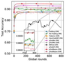
(a)

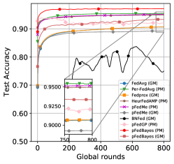
(b)

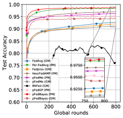
(c)

Figure 2: Comparison results of the convergence rate of different algorithms on the MNIST dataset. Left: Small dataset. Middle: Medium dataset. Right: Large dataset.

5 Experiments

5.1 Experimental Setting

We compare the performance of the proposed method pFedBayes with FedAvg (McMahan et al., 2017), Fedprox (Li et al., 2018), BNFed (Yurochkin et al., 2019), Per-FedAvg (Fallah et al., 2020), pFedMe (T Dinh et al., 2020), HeurFedAMP (Huang et al., 2021) and pFedGP (Achituve et al., 2021) based on non-i.i.d. datasets. We generate the non-i.i.d. datasets based on three public benchmark datasets, MNIST (LeCun et al., 2010, 1998), FMNIST (Fashion-MNIST)(Xiao et al., 2017) and CIFAR-10 (Krizhevsky, 2009). For MNIST, FMNIST and CIFAR-10 datasets, we follow the non-i.i.d. setting strategy in (T Dinh et al., 2020). Each client occupies a unique local data and only has 5 of the 10 labels. The number of clients for MNIST/FMNIST datasets is set as 10, while the number of clients for CIFAR-10 dataset is set as 20.

In addition, we split small, medium and large datasets on each public dataset to further validate the performance of our algorithm. For small, medium and large datasets of MNIST/FMNIST, there were 50, 200, 900 training samples and 950, 800, 300 test samples for each class, respectively. For the small, medium and large datasets of CIFAR-10, there were 25, 100, 450 training samples and 475, 400, 150 test samples in each class, respectively. For the random subset of clients $S$, we set $S=10$ for experiments on MNIST, FMNIST and CIFAR-10 datasets. We evaluate the performance of all algorithms by computing the highest accuracy over 700 to 800 communication rounds.

We did all experiments in this paper using servers with two GPUs (NVIDIA Tesla P100 with 16GB memory), two CPUs (each with 22 cores, Intel(R) Xeon(R) Gold 6152 CPU @ 2.10GHz), and 192 GB memory. The base DNN and VGG models and federated learning environment are implemented according to the settings in (T Dinh et al., 2020). In particular, the DNN model uses one hidden layer, ReLU activation, and a softmax layer at the end. For the MNIST and FMNIST datasets, the size of the hidden layer is 100. The VGG model (Simonyan & Zisserman, 2014) is implemented for CIFAR-10 dataset with “[16, ‘M’, 32, ‘M’, 64, ‘M’, 128, ‘M’, 128, ‘M’]” cfg setting. We use PyTorch (Paszke et al., 2019) for all experiments.

5.2 Experimental Hyperparameter Settings

We first investigate the impact of hyperparameters on all algorithms based on the medium MNIST dataset and try to find the best hyperparameter settings for each algorithm to fairly compare their performance. For all hyperparameters, we refer to the settings in the corresponding papers of each algorithm and tune the parameters around their recommended values. For example, many algorithms use a learning rate $\eta=0.005$ (e.g., pFedMe), then we set the learning rate in the range of 0.0005 to 0.1 for parameter tuning. For some algorithm-specific hyperparameters, we use the values recommended in their papers. More detailed results of parameter tuning are given in Appendix B.

Based on the experimental results, we set the learning rate of FedAvg and Per-FedAvg to 0.01. The learning rate and regularization weight of Fedprox are respectively set as 0.01 and $\lambda=0.001$. The learning rate of BNFed is set as 0.5, while for pFedGP is set as 0.05. The personalized learning rate, global learning rate and regularization weight of pFedMe are respectively set as 0.01, 0.01 and $\lambda=15$. The learning rate and regularization weight of HeurFedAMP are respectively set as 0.01 and $\alpha=5$. For the proposed pFedBayes, we set the initialization of weight parameters $\rho=-2.5$, the tradeoff parameter $\zeta=10$, and the learning rates of the personalized model and global model $\eta_{1}=\eta_{2}=0.001$.

5.3 Performance Comparison Results

Table 1 shows the performance of each algorithm under the optimal hyperparameter settings. On small, medium and large datasets of MNIST, the personalized model of our algorithm outperforms other SOTA comparison algorithms by 1.25$\%$, 1.78$\%$ and 0.52$\%$, while the global model outperforms other SOTA models by 2.79$\%$, 1.67$\%$ and 1.97$\%$, respectively. We can see that our algorithm performs better when the amount of data is small, thanks to the advantage of the Bayesian algorithm on small samples. Figure 2 shows the comparison results of the convergence speed of different algorithms on the MNIST dataset. We can see that our pFedBayes converges significantly under a small dataset, and the performance is stable after 50 iterations, clearly ahead of other algorithms.

On the small, medium and large datasets of FMNIST, the personalization model of our algorithm outperforms other SOTA comparison algorithms by 0.42$\%$, 0.63$\%$ and 0.79$\%$, respectively. However, the accuracy of the global model is not ahead. This is mainly because the FMNIST dataset is relatively simple and does not have good non-i.i.d. features. Therefore, the advantages of personalization algorithms are not obvious. This can be verified by the fact that FedAvg achieves optimal performance on large datasets.

On the small, medium and large datasets of CIFAR-10, the personalization model of our algorithm respectively outperforms other SOTA comparison algorithms by 11.71$\%$. 7.19$\%$ and 6.33$\%$. It can be seen that for complex non-i.i.d. dataset, our pFedBayes can achieve substantial improvement on small samples. The global model also outperforms other SOTA models by 3.47$\%$ and 3.49$\%$ on small and medium datasets, respectively. But on large datasets, our global model has no performance advantage. This is because the excellent performance of pFedBayes under small samples is attributed to BNN (Blundell et al., 2015b; Khan, 2019). For large datasets, BNNs need other techniques to achieve the same performance as non-Bayesian algorithms (Osawa et al., 2019). For fairness, we use the same techniques in large datasets as that in small datasets, resulting in performance degradation when aggregating models.

Furthermore, our pFedBayes can provide results for model uncertainty estimation, a useful information in federated learning. See Appendix B.2 for more detailed results.

6 Conclusions

In this paper, we propose a novel personalized federated learning model via variational Bayesian inference. Each client uses the aggregated global distribution as prior distribution and updates its personal distribution by balancing the construction error over its personal data and the KL divergence with aggregated global distribution. We provide theoretical analysis for the averaged generalization error of all clients, which shows that the proposed model achieves minimax-rate optimality up to a logarithmic factor. An efficient algorithm is given by updating the global model and personal models alternatively. Extensive experiments present that the proposed algorithm outperforms many advanced personalization methods in most cases, especially when the amount of data is limited.

Appendix A Proof of Lemmas

A.1 Proof of Lemma 1

Before prove Lemma 1, let’s review an important lemma. Lemma A.1 restates the Donsker and Varadhan’s representation for the KL divergence, whose proof can be found in (Boucheron et al., 2013).

Lemma A.1.

For any probability measure $\mu$ and any measurable function $h$ with $e^{h}\in L_{1}(\mu)$,

$$\log\int e^{h(\eta)}\mu(d\eta)=\sup_{\rho}\left[\int h(\eta)\rho(d\eta)-\mbox{\rm KL}(\rho||\mu)\right].$$

Now we are ready to prove Lemma 1. Let $\log\eta(P^{i}_{\bm{\theta}},P^{i})=l_{n}(P^{i}_{\bm{\theta}},P^{i})/\zeta+n\,d^{2}(P^{i}_{\bm{\theta}},P^{i})$. Since $\zeta\geq 1$, using Jensen’s inequality and the concavity of $(\cdot)^{1/\zeta}$ gets

$$\mathbb{E}_{P^{i}}\exp(l_{n}(P^{i}_{\bm{\theta}},P^{i})/\zeta)=\mathbb{E}_{P^{i}}\left(\frac{p^{i}_{\bm{\theta}}(\bm{D}^{i})}{p^{i}(\bm{D}^{i})}\right)^{\frac{1}{\zeta}}\leq\left(\mathbb{E}_{P^{i}}\frac{p^{i}_{\bm{\theta}}(\bm{D}^{i})}{p^{i}(\bm{D}^{i})}\right)^{\frac{1}{\zeta}}=1.$$ (A.1)

Together with the proof from the Theorem 3.1 of (Pati et al., 2018), we have

$$\int_{\Theta}\eta(P^{i}_{\bm{\theta}},P^{i})w^{\star}(\bm{\theta})d\bm{\theta}\leq e^{Cn\varepsilon^{2}_{n}},\,\mbox{w.h.p.,}$$ (A.2)

where $C>0$ is a large constant.

By using Lemma A.1 with $h(\eta)=\log\eta(P^{i}_{\bm{\theta}},P^{i})$, $\mu=w^{\star}(\bm{\theta})$ and $\rho=\hat{q}^{i}(\bm{\theta})$, we obtain

$$\int_{\Theta}d^{2}(P_{\bm{\theta}}^{i},P^{i})\hat{q}^{i}(\bm{\theta})d\bm{\theta}\leq \frac{1}{n}\left[\frac{1}{\zeta}\int_{\Theta}l_{n}(P^{i},P^{i}_{\bm{\theta}})\hat{q}^{i}(\bm{\theta})d\bm{\theta}+\mbox{KL}(\hat{q}^{i}(\bm{\theta})||w^{\star}(\bm{\theta}))+\log\int_{\Theta}\eta(P^{i}_{\bm{\theta}},P^{i})w^{\star}(\bm{\theta})d\bm{\theta}\right]$$

$$\leq \frac{1}{n}\left[\frac{1}{\zeta}\int_{\Theta}l_{n}(P^{i},P^{i}_{\bm{\theta}})\hat{q}^{i}(\bm{\theta})d\bm{\theta}+\mbox{KL}(\hat{q}^{i}(\bm{\theta})||w^{\star}(\bm{\theta}))\right]+C\varepsilon^{2}_{n}.$$ (A.3)

By averaging over all $N$ clients, we have

$$\frac{1}{N}\sum_{i=1}^{N}\int_{\Theta}d^{2}(P_{\bm{\theta}}^{i},P^{i})\hat{q}^{i}(\bm{\theta})d\bm{\theta}\leq\frac{1}{n}\left\{\frac{1}{N}\sum_{i=1}^{N}\left[\frac{1}{\zeta}\int_{\Theta}l_{n}(P^{i},P^{i}_{\bm{\theta}})\hat{q}^{i}(\bm{\theta})d\bm{\theta}+\mbox{KL}(\hat{q}^{i}(\bm{\theta})||w^{\star}(\bm{\theta}))\right]\right\}+C\varepsilon^{2}_{n}.$$ (A.4)

A.2 Proof of Lemma 2

Before prove Lemma 2, we present a lemma to give the optimal $w(\bm{\theta})$ for given distribution of each client $q^{i}(\bm{\theta})$, which is proved in Section A.3.

Lemma A.2.

Let $w(\bm{\theta})$ be the optimal variational solution of the problem

$$\min_{w(\bm{\theta})}\left\{F(w)=\frac{1}{N}\sum_{i=1}^{N}\mbox{\rm KL}(q^{i}(\bm{\theta})||w(\bm{\theta})))\right\}.$$ (A.5)

Then we have

$$\mu_{w,m} =\frac{1}{N}\sum_{i=1}^{N}\mu_{i,m},$$ (A.6)

$$\sigma_{w,m}^{2} =\frac{1}{N}\sum_{i=1}^{N}\left[\sigma_{i,m}^{2}+\left(\mu_{i,m}-\mu_{w,m}\right)^{2}\right]=\frac{1}{N}\sum_{i=1}^{N}\left[\sigma_{i,m}^{2}+\mu_{i,m}^{2}-\mu_{w,m}^{2}\right].$$ (A.7)

Now we are ready to prove Lemma 2. Choosing $\bm{\theta}^{\star}_{i}$ that minimizes $\left\lVert f^{i}_{\bm{\theta}}-f^{i}\right\rVert^{2}_{\infty}$ subject to $\left\lVert\bm{\theta}\right\rVert_{\infty}\leq B$, then we define $\tilde{q}^{i}(\bm{\theta})$ as follows, for $m=1,\dots,T$:

$$\begin{split}&\theta_{i,m}\sim\mathcal{N}(\theta_{i,m}^{\star},\sigma^{2}_{n}),\end{split}$$ (A.8)

where

$$\sigma_{n}^{2}=\frac{T}{8n}A$$ (A.9)

and

$$A=\log^{-1}(3s_{0}M)\cdot(2BM)^{-2(L+1)}\left[\left(s_{0}+1+\frac{1}{BM-1}\right)^{2}+\frac{1}{(2BM)^{2}-1}+\frac{2}{(2BM-1)^{2}}\right]^{-1}.$$ (A.10)

Let $\tilde{w}(\bm{\theta})$ be the optimal solution for

$$\min_{w(\bm{\theta})\in\mathcal{Q}}\frac{1}{N}\sum_{i=1}^{N}\mbox{KL}(\tilde{q}^{i}(\bm{\theta})||w(\bm{\theta}))).$$ (A.11)

Then by using Lemma A.2, the distribution $\tilde{w}(\bm{\theta})$ satisfies

$$\theta_{\tilde{w},m}\sim\mathcal{N}(\mu_{\tilde{w},m},\sigma^{2}_{\tilde{w},m}),m=1,\ldots,T,$$ (A.12)

where

$$\mu_{\tilde{w},m} =\frac{1}{N}\sum_{i=1}^{N}\theta_{i,m}^{\star},$$ (A.13)

$$\sigma_{\tilde{w},m}^{2} =\frac{1}{N}\sum_{i=1}^{N}\left[\sigma_{n}^{2}+\left(\theta_{i,m}^{\star}-\mu_{\tilde{w},m}\right)^{2}\right]=\sigma_{n}^{2}-\mu_{\tilde{w},m}^{2}+\frac{1}{N}\sum_{i=1}^{N}\theta_{i,m}^{\star 2}.$$ (A.14)

Since $w^{\star}(\bm{\theta})$ and $\hat{q}(\bm{\theta})$ correspond to the optimal solution of the global problem, then we obtain

$$\frac{1}{N}\sum_{i=1}^{N}\left[\int_{\Theta}l_{n}(P^{i},P^{i}_{\bm{\theta}})\hat{q}^{i}(\bm{\theta})d\bm{\theta}+\zeta\,\mbox{KL}(\hat{q}^{i}(\bm{\theta})||w^{\star}(\bm{\theta}))\right]\\ \leq\frac{1}{N}\sum_{i=1}^{N}\left[\int_{\Theta}l_{n}(P^{i},P^{i}_{\bm{\theta}})\tilde{q}^{i}(\bm{\theta})d\bm{\theta}+\zeta\,\mbox{KL}(\tilde{q}^{i}(\bm{\theta})||\tilde{w}(\bm{\theta}))\right].$$ (A.15)

Next we will give the upper bound under probability distributions $\tilde{w}(\bm{\theta})$ and $\tilde{q}^{i}(\bm{\theta})$. According to the definitions above and the mean-field decomposition, we can represent the probabilities as follows

$$\tilde{q}^{i}(\bm{\theta})=\prod^{T}_{m=1}\mathcal{N}(\theta^{\star}_{i,m},\sigma^{2}_{n}),$$ (A.16)

$$\tilde{w}(\bm{\theta})=\prod^{T}_{m=1}\mathcal{N}(\mu_{\tilde{w},m},\sigma^{2}_{\tilde{w},m}).$$ (A.17)

Then we have

$$\mbox{KL}(\tilde{q}^{i}(\bm{\theta})||\tilde{w}(\bm{\theta}))= \mbox{KL}\left(\prod^{T}_{m=1}\mathcal{N}(\theta^{\star}_{i,m},\sigma^{2}_{n})\Bigl{|}\Bigr{|}\prod^{T}_{m=1}\mathcal{N}(\mu_{\tilde{w},m},\sigma^{2}_{\tilde{w},m})\right)$$

$$= \sum^{T}_{m=1}\mbox{KL}\left(\mathcal{N}(\theta^{\star}_{i,m},\sigma^{2}_{n})||\mathcal{N}(\mu_{\tilde{w},m},\sigma^{2}_{\tilde{w},m})\right)$$

$$= \frac{1}{2}\sum^{T}_{m=1}\left[\log\Bigl{(}\frac{\sigma^{2}_{\tilde{w},m}}{\sigma^{2}_{n}}\Bigr{)}+\frac{\sigma^{2}_{n}+(\theta^{\star}_{i,m}-\mu_{\tilde{w},m})^{2}}{\sigma^{2}_{\tilde{w},m}}-1\right]$$

$$= \frac{1}{2}\sum^{T}_{m=1}\left[\log\Bigl{(}\frac{\sigma^{2}_{\tilde{w},m}}{\sigma^{2}_{n}}\Bigr{)}-1\right]+\frac{1}{2}\sum^{T}_{m=1}\frac{\sigma^{2}_{n}+(\theta^{\star}_{i,m}-\mu_{\tilde{w},m})^{2}}{\sigma^{2}_{\tilde{w},m}}$$

$$\leq \frac{T}{2}\left[\log\left(\frac{\sigma^{2}_{n}+B^{2}}{\sigma^{2}_{n}}\right)-1\right]+\frac{1}{2}\sum^{T}_{m=1}\frac{\sigma^{2}_{n}+(\theta^{\star}_{i,m}-\mu_{\tilde{w},m})^{2}}{\sigma^{2}_{\tilde{w},m}},$$ (A.18)

where the inequality applies

$$\sigma_{\tilde{w},m}^{2}=\sigma_{n}^{2}-\mu_{\tilde{w},m}^{2}+\frac{1}{N}\sum_{i=1}^{N}\theta_{i,m}^{\star 2}\leq\sigma^{2}_{n}+B^{2}.$$

So the sum of the KL divergence (A.2) satisfies

$$\frac{1}{N}\sum_{i=1}^{N}\mbox{KL}(\tilde{q}^{i}(\bm{\theta})||\tilde{w}(\bm{\theta})) \leq\frac{1}{N}\sum_{i=1}^{N}\left\{\frac{T}{2}\left[\log\left(\frac{\sigma^{2}_{n}+B^{2}}{\sigma^{2}_{n}}\right)-1\right]+\frac{1}{2}\sum^{T}_{m=1}\frac{\sigma^{2}_{n}+(\theta^{\star}_{i,m}-\mu_{\tilde{w},m})^{2}}{\sigma^{2}_{\tilde{w},m}}\right\}$$

$$\leq\frac{T}{2}\log\left(\frac{\sigma^{2}_{n}+B^{2}}{\sigma^{2}_{n}}\right),$$

where the last inequality applies (A.14) such that

$$\frac{1}{N}\sum_{i=1}^{N}\frac{\sigma^{2}_{n}+(\theta^{\star}_{i,m}-\mu_{\tilde{w},m})^{2}}{\sigma^{2}_{\tilde{w},m}}=1.$$

Under Assumption 3, we obtain

$$\frac{1}{N}\sum_{i=1}^{N}\mbox{KL}(\tilde{q}^{i}(\bm{\theta})||\tilde{w}(\bm{\theta}))\leq\frac{T}{2}\log\left(\frac{2B^{2}}{\sigma^{2}_{n}}\right).$$ (A.19)

Incorporating the definition of $\sigma_{n}$ yields the following result

$$\frac{T}{2}\log\left(\frac{2B^{2}}{\sigma^{2}_{n}}\right)\leq T(L+1)\log(2BM)+\frac{T}{2}\log\log(3s_{0}M)+T\log\left(4s_{0}\sqrt{\frac{n}{T}}\right)+\frac{T}{2}\log(2B^{2})\leq C^{\prime}nr_{n}.$$

Therefore, we get

$$\frac{1}{N}\sum_{i=1}^{N}\mbox{KL}(\tilde{q}^{i}(\bm{\theta})||\tilde{w}(\bm{\theta}))\leq C^{\prime}nr_{n}.$$ (A.20)

By following the technique from the Supplementary of (Bai et al., 2020), we can give the following upper bound

$$\int_{\Theta}l_{n}(P^{i},P^{i}_{\bm{\theta}})\tilde{q}^{i}(\bm{\theta})d\bm{\theta}\leq C^{\prime\prime}(nr_{n}+n\xi^{i}_{n}).$$ (A.21)

Combining the above results and $\zeta\geq 1$ gives that

$$\frac{1}{N}\sum_{i=1}^{N}\left[\int_{\Theta}l_{n}(P^{i},P^{i}_{\bm{\theta}})\hat{q}^{i}(\bm{\theta})d\bm{\theta}+\zeta\,\mbox{KL}(\hat{q}^{i}(\bm{\theta})||w^{\star}(\bm{\theta}))\right]\leq n\left(C^{\prime}\zeta r_{n}+\frac{C^{\prime\prime}}{N}\sum_{i=1}^{N}\xi^{i}_{n}\right).$$ (A.22)

A.3 Proof of Lemma A.2

Since $w(\bm{\theta})$ is the optimal solution of Eq. (A.5), the partial derivatives of $F(w)$ with respect to $\mu_{w,m}$ and $\sigma_{w,m}$ are zero, i.e.,

$$\frac{1}{N}\sum_{i=1}^{N}\frac{\partial\,\mbox{KL}(q^{i}(\bm{\theta})||w(\bm{\theta}))}{\partial\,\mu_{w,m}} =0,$$ (A.23)

$$\frac{1}{N}\sum_{i=1}^{N}\frac{\partial\,\mbox{KL}(q^{i}(\bm{\theta})||w(\bm{\theta}))}{\partial\,\sigma_{w,m}} =0.$$ (A.24)

According to Eq. (2), we can get the partial derivatives

$$\frac{1}{N}\sum_{i=1}^{N}\frac{\partial\,\mbox{KL}(q^{i}(\bm{\theta})||w(\bm{\theta}))}{\partial\,\mu_{w,m}} =\frac{1}{N}\sum_{i=1}^{N}\frac{-2(\mu_{i,m}-\mu_{w,m})}{\sigma_{w,m}^{2}},$$ (A.25)

$$\frac{1}{N}\sum_{i=1}^{N}\frac{\partial\,\mbox{KL}(q^{i}(\bm{\theta})||w(\bm{\theta}))}{\partial\,\sigma_{w,m}} =\frac{1}{N}\sum_{i=1}^{N}\left[\frac{2}{\sigma_{w,m}}-\frac{2\left[\sigma_{i,m}^{2}+\left(\mu_{i,m}-\mu_{w,m}\right)^{2}\right]}{\sigma_{w,m}^{3}}\right].$$ (A.26)

Combining Eqs. (A.23), (A.24), (A.25) and (A.26) yields

$$\mu_{w,m} =\frac{1}{N}\sum_{i=1}^{N}\mu_{i,m},$$ (A.27)

$$\sigma_{w,m}^{2} =\frac{1}{N}\sum_{i=1}^{N}\left[\sigma_{i,m}^{2}+\left(\mu_{i,m}-\mu_{w,m}\right)^{2}\right]$$

$$=\frac{1}{N}\sum_{i=1}^{N}\left[\sigma_{i,m}^{2}+\mu_{i,m}^{2}-\mu_{w,m}^{2}\right].$$ (A.28)

Appendix B Experimental Results on MNIST Dataset

B.1 Effect of Hyperparameters

We test pFedBayes in a basic DNN model with 3 full connection layers [784, 100, 10] on the MNIST dataset. The results are listed in Table 2. Effects of $\eta_{1}$ and $\eta_{2}$: In pFedBayes algorithm, $\eta_{1}$ and $\eta_{2}$ are respectively denote the learning rate of the personalized model and global model. We tune the learning rate in the range of $[0.001,0.005]$ while fix other parameters. From Table 2 we can see that $\eta_{1}=\eta_{2}=0.001$ is the best setting. Effects of $\zeta$: In pFedBayes algorithm, $\zeta$ can adjust the degree of personalization of personalized models. Increasing $\zeta$ can improve the test accuracy of the global model and weaken the performance of the personalized model. On the basis of the best learning rate, we tune $\zeta\in\{0.5,1,5,10,20\}$. Table 2 shows that $\zeta=10$ is the best setting. Hence, we set $\zeta=10$ for the remaining experiments. Effects of $\rho$: It is known that the initialization of the weight parameters affects the results of the model. Hence, we also tune $\rho\in\{-1,-1.5,-2,-2.5,-3\}$. Table 2 shows that $\rho=-2.5$ is the best setting. Hence, we set $\rho=-2.5$ for the remaining experiments.

The results of FedAvg, Fedprox, NBFed, Per-FedAvg, pFedMe, HeurFedAMP and pFedGP are listed in Table 3. The parameters $\eta_{1}$ and $\eta_{2}$ are the learning rates of the personalized model and the global model, respectively. “Personalized” means this column indicates whether this is a personalized algorithm. In order to make a fair comparison with these algorithms, we perform the following hyperparameter adjustment. In (T Dinh et al., 2020), $\lambda=15$ achieves the best performance and is the recommended setting, so we use this setting directly in our experiments. We tune $\lambda\in\{0.001,0.01,0.1,1\}$ the same as the setting in Fedprox (Li et al., 2018). For HeurFedAMP , we tune $\alpha\in[0.1,0.5]$, and $0.5$ is the recommended setting in its paper (Huang et al., 2021). For pFedGP, the recommended learning rate in its paper is 0.05, we hence tune $\eta\in[0.01,0.05,0.1]$. We can see that $\eta=0.05$ can achieve better performance. For other hyperparameters in pFedGP, we set them the same as in (Achituve et al., 2021). Notably, $\alpha$ represents the proportion of the client model that does not interact with the global model. The higher the value, the less interaction with the global model. For other algorithms, there are 10 client models interacting with the global model. For a fair comparison, the corresponding $\alpha$ should be set to 0.1. Clearly 0.5 provides better performance of the personalized model, although a setting of 0.5 is not a fair comparison. We still use the parameter setting of 0.5 recommended in its paper. In addition, it should be noted that the learning rate cannot be set too large, and an appropriate value should be taken. For most federated learning algorithms, a learning rate that is too large will cause the model to diverge, resulting in a severe loss of model aggregation performance. From the experimental results of the personalized algorithms, we find that the optimal learning rate is between 0.0005 and 0.01. For a fair comparison, we also set the learning rates of the non-personalized algorithms, i.e. FedAvg and FedProx, within this range.

Table 2: Results of pFedBayes on Medium dataset (MNIST).

$\rho$	$\zeta$	$\eta_{1}$	$\eta_{2}$	PM Acc.($\%$)	GM Acc.($\%$)
-1	10	0.001	0.001	97.38	91.61
-1	10	0.001	0.005	97.12	90.32
-1	10	0.005	0.001	96.73	91.34
-1	10	0.005	0.005	96.78	91.10
-2	10	0.001	0.001	97.45	92.40
-2	10	0.001	0.005	97.42	91.35
-2	10	0.005	0.001	97.36	91.27
-2	10	0.005	0.005	97.28	90.01
-3	10	0.001	0.001	97.08	92.16
-3	10	0.001	0.005	96.35	90.47
-3	10	0.005	0.001	96.64	87.34
-3	10	0.005	0.005	97.28	90.22
-1.5	10	0.001	0.001	97.38	92.31
-2.0	10	0.001	0.001	97.45	92.40
-2.5	10	0.001	0.001	97.18	93.22
-2.5	0.5	0.001	0.001	97.13	89.88
-2.5	1	0.001	0.001	97.41	91.24
-2.5	5	0.001	0.001	97.38	93.03
-2.5	10	0.001	0.001	97.18	93.22
-2.5	20	0.001	0.001	97.04	92.77

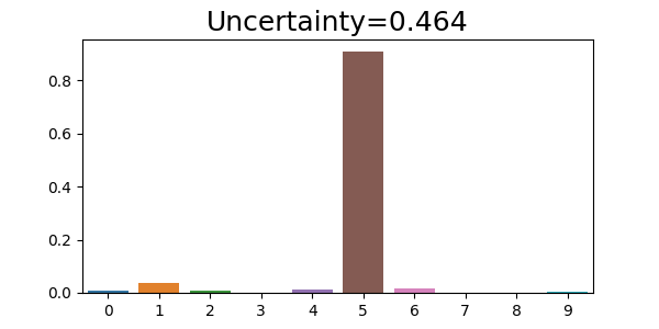
(a)

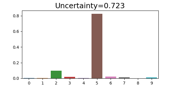
(b)

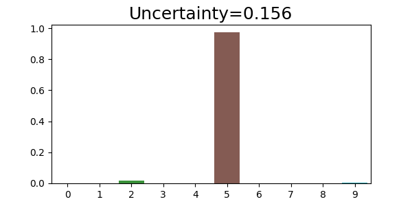
(c)

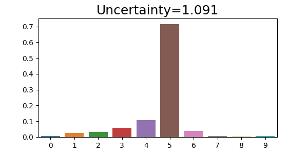
(d)

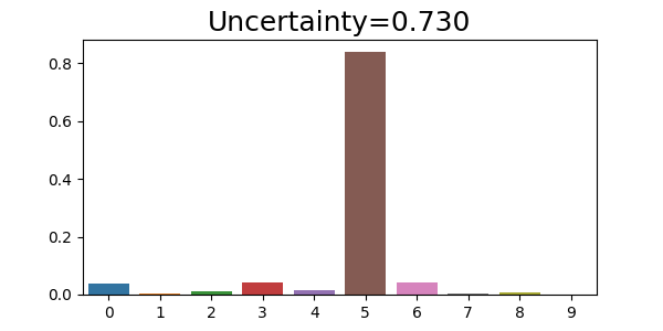
(e)

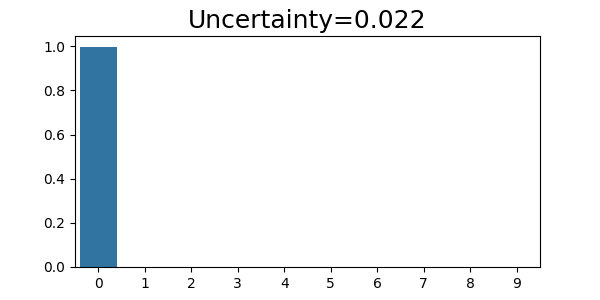
(f)

(g)

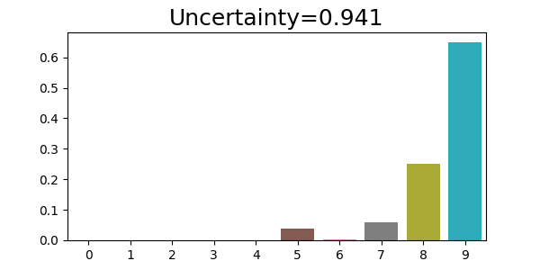
(h)

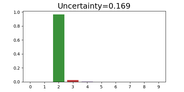
(i)

(j)

(k)

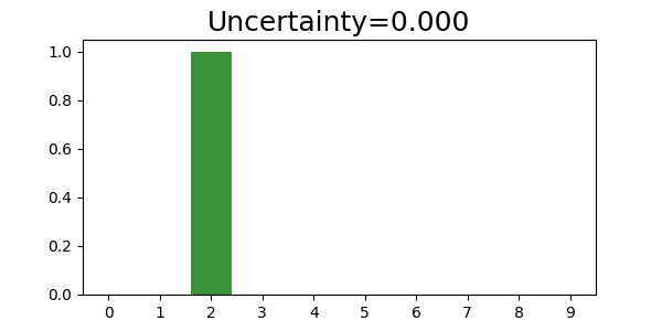
(l)

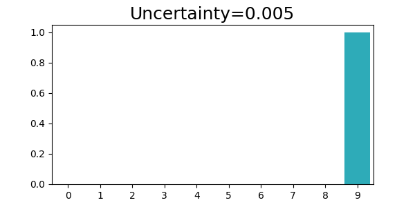
(m)

(n)

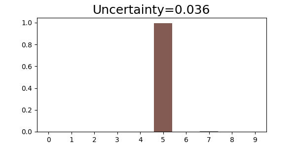
(o)

Figure 3: Predication uncertainty of personalized Bayesian federated learning model with Gaussian assumptions. From the first row to the third row, the number of training rounds is 0, 1, and 10, respectively. The five columns represent five different clients.

Table 3: Comparison algorithm results on the medium dataset (MNIST).

Algorithm	$\eta_{1}$	$\eta_{2}$	$\lambda$	$\alpha$	PM Acc.(%)	GM Acc.(%)	Personalized
pFedMe	0.0005	0.001	15	-	83.22	80.86	Y
pFedMe	0.001	0.001	15	-	89.35	86.86	Y
pFedMe	0.005	0.005	15	-	94.35	89.17	Y
pFedMe	0.01	0.01	15	-	95.16	89.31	Y
pFedMe	0.1	0.1	15	-	19.73	9.9	Y
HeurFedAMP	0.0005	-	-	0.1	89.73	-	Y
HeurFedAMP	0.001	-	-	0.1	89.91	-	Y
HeurFedAMP	0.005	-	-	0.1	89.41	-	Y
HeurFedAMP	0.01	-	-	0.1	88.68	-	Y
HeurFedAMP	0.1	-	-	0.1	10.03	-	Y
HeurFedAMP	0.0005	-	-	0.5	93.32	-	Y
HeurFedAMP	0.001	-	-	0.5	94.04	-	Y
HeurFedAMP	0.005	-	-	0.5	94.90	-	Y
HeurFedAMP	0.01	-	-	0.5	94.95	-	Y
HeurFedAMP	0.1	-	-	0.5	93.29	-	Y
Per-FedAvg	0.0005	-	-	-	94.71	-	Y
Per-FedAvg	0.001	-	-	-	94.95	-	Y
Per-FedAvg	0.005	-	-	-	95.31	-	Y
Per-FedAvg	0.01	-	-	-	95.35	-	Y
Per-FedAvg	0.1	-	-	-	19.94	-	Y
pFedGP	0.01	-	-	-	90.52	-	Y
pFedGP	0.05	-	-	-	92.14	-	Y
pFedGP	0.1	-	-	-	91.23	-	Y
FedAvg	-	0.0005	-	-	-	87.65	N
FedAvg	-	0.001	-	-	-	89.19	N
FedAvg	-	0.005	-	-	-	90.08	N
FedAvg	-	0.01	-	-	-	90.66	N
Fedprox	-	0.001	0.001	-	-	89.26	N
Fedprox	-	0.001	0.01	-	-	89.24	N
Fedprox	-	0.001	0.1	-	-	87.79	N
Fedprox	-	0.001	1	-	-	76.79	N
Fedprox	-	0.0005	0.001	-	-	87.64	N
Fedprox	-	0.001	0.001	-	-	89.26	N
Fedprox	-	0.005	0.001	-	-	89.84	N
Fedprox	-	0.01	0.001	-	-	90.70	N
BNFed	-	0.0005	-	-	-	9.90	N
BNFed	-	0.001	-	-	-	9.90	N
BNFed	-	0.005	-	-	-	9.90	N
BNFed	-	0.01	-	-	-	9.94	N
BNFed	-	0.1	-	-	-	55.98	N
BNFed	-	0.2	-	-	-	74.47	N
BNFed	-	0.5	-	-	-	80.31	N

B.2 pFedBayes Uncertainty Estimation

One of the advantages of Bayesian algorithm is that it can provide uncertainty estimation results. Figure 3 shows that the predication uncertainty of personalized model of our pFedBayes. We can see that random model parameters do not give accurate estimates before training. As training progresses, the model becomes more and more confident in the classification results. The results of uncertainty estimation can give people a good reference, especially in federated learning architectures. When aggregating models, we can know the uncertainty of each client model. This information can be used to evaluate the quality of the client model, decide whether to aggregate, etc.

References

- Achituve et al. (2021) Achituve, I., Shamsian, A., Navon, A., Chechik, G., and Fetaya, E. Personalized federated learning with gaussian processes. In Thirty-Fifth Conference on Neural Information Processing Systems, 2021.
- Al-Shedivat et al. (2021) Al-Shedivat, M., Gillenwater, J., Xing, E., and Rostamizadeh, A. Federated learning via posterior averaging: A new perspective and practical algorithms. In International Conference on Learning Representations, 2021.
- Alquier & Ridgway (2020) Alquier, P. and Ridgway, J. Concentration of tempered posteriors and of their variational approximations. The Annals of Statistics, 48(3):1475–1497, 2020.
- Arivazhagan et al. (2019) Arivazhagan, M. G., Aggarwal, V., Singh, A. K., and Choudhary, S. Federated learning with personalization layers. arXiv preprint arXiv:1912.00818, 2019.
- Bai et al. (2020) Bai, J., Song, Q., and Cheng, G. Efficient variational inference for sparse deep learning with theoretical guarantee. Advances in Neural Information Processing Systems, 33, 2020.
- Blei et al. (2017) Blei, D. M., Kucukelbir, A., and McAuliffe, J. D. Variational inference: A review for statisticians. Journal of the American Statistical Association, 112(518):859–877, 2017.
- Blundell et al. (2015a) Blundell, C., Cornebise, J., Kavukcuoglu, K., and Wierstra, D. Weight uncertainty in neural networks. In Proceedings of the 32Nd International Conference on International Conference on Machine Learning - Volume 37, ICML’15, pp. 1613–1622. JMLR.org, 2015a.
- Blundell et al. (2015b) Blundell, C., Cornebise, J., Kavukcuoglu, K., and Wierstra, D. Weight uncertainty in neural network. In International Conference on Machine Learning, pp. 1613–1622. PMLR, 2015b.
- Boucheron et al. (2013) Boucheron, S., Lugosi, G., and Massart, P. Concentration inequalities: A nonasymptotic theory of independence. Oxford university press, 2013.
- Chen et al. (2018) Chen, F., Luo, M., Dong, Z., Li, Z., and He, X. Federated meta-learning with fast convergence and efficient communication. arXiv preprint arXiv:1802.07876, 2018.
- Chen & Chao (2021) Chen, H.-Y. and Chao, W.-L. FedBE: Making Bayesian model ensemble applicable to federated learning. In International Conference on Learning Representations, 2021.
- Chérief-Abdellatif (2020) Chérief-Abdellatif, B.-E. Convergence rates of variational inference in sparse deep learning. In International Conference on Machine Learning, pp. 1831–1842. PMLR, 2020.
- Chérief-Abdellatif & Alquier (2018) Chérief-Abdellatif, B.-E. and Alquier, P. Consistency of variational bayes inference for estimation and model selection in mixtures. Electronic Journal of Statistics, 12(2):2995–3035, 2018.
- Dai et al. (2019) Dai, X., Yan, X., Zhou, K., Yang, H., Ng, K. K., Cheng, J., and Fan, Y. Hyper-sphere quantization: Communication-efficient sgd for federated learning. arXiv preprint arXiv:1911.04655, 2019.
- Fallah et al. (2020) Fallah, A., Mokhtari, A., and Ozdaglar, A. Personalized federated learning with theoretical guarantees: A model-agnostic meta-learning approach. Advances in Neural Information Processing Systems, 33:3557–3568, 2020.
- Guha et al. (2019) Guha, N., Talwalkar, A., and Smith, V. One-shot federated learning. arXiv preprint arXiv:1902.11175, 2019.
- Hanzely & Richtárik (2020) Hanzely, F. and Richtárik, P. Federated learning of a mixture of global and local models. arXiv preprint arXiv:2002.05516, 2020.
- Higgins et al. (2017) Higgins, I., Matthey, L., Pal, A., Burgess, C., Glorot, X., Botvinick, M., Mohamed, S., and Lerchner, A. Beta-VAE: Learning basic visual concepts with a constrained variational framework. In International Conference on Learning Representations, 2017.
- Huang et al. (2021) Huang, Y., Chu, L., Zhou, Z., Wang, L., Liu, J., Pei, J., and Zhang, Y. Personalized cross-silo federated learning on non-iid data. In Proceedings of the AAAI Conference on Artificial Intelligence, volume 35, pp. 7865–7873, 2021.
- Jordan et al. (1999) Jordan, M. I., Ghahramani, Z., Jaakkola, T. S., and Saul, L. K. An introduction to variational methods for graphical models. Machine Learning, 37:183–233, 1999.
- Jospin et al. (2020) Jospin, L. V., Buntine, W., Boussaid, F., Laga, H., and Bennamoun, M. Hands-on bayesian neural networks-a tutorial for deep learning users. ACM Comput. Surv, 1(1), 2020.
- Karimireddy et al. (2020) Karimireddy, S. P., Kale, S., Mohri, M., Reddi, S., Stich, S., and Suresh, A. T. Scaffold: Stochastic controlled averaging for federated learning. In International Conference on Machine Learning, pp. 5132–5143. PMLR, 2020.
- Khan (2019) Khan, M. E. Deep learning with bayesian principles. Tutorial on Advances in Neural Information Processing Systems, 2019.
- Krizhevsky (2009) Krizhevsky, A. Learning multiple layers of features from tiny images. Master’s thesis, University of Tront, 2009.
- LeCun et al. (1998) LeCun, Y., Bottou, L., Bengio, Y., and Haffner, P. Gradient-based learning applied to document recognition. Proceedings of the IEEE, 86(11):2278–2324, 1998.
- LeCun et al. (2010) LeCun, Y., Cortes, C., and Burges, C. Mnist handwritten digit database. ATT Labs [Online]. Available: http://yann.lecun.com/exdb/mnist, 2, 2010.
- Li et al. (2018) Li, T., Sahu, A. K., Zaheer, M., Sanjabi, M., Talwalkar, A., and Smith, V. Federated optimization in heterogeneous networks. arXiv preprint arXiv:1812.06127, 2018.
- Li et al. (2019) Li, T., Sahu, A. K., Zaheer, M., Sanjabi, M., Talwalkar, A., and Smithy, V. Feddane: A federated newton-type method. In 2019 53rd Asilomar Conference on Signals, Systems, and Computers, pp. 1227–1231. IEEE, 2019.
- Li et al. (2020) Li, T., Sahu, A. K., Talwalkar, A., and Smith, V. Federated learning: Challenges, methods, and future directions. IEEE Signal Processing Magazine, 37(3):50–60, 2020.
- Li et al. (2022a) Li, X.-C., Xu, Y.-C., Song, S., Li, B., Li, Y., Shao, Y., and Zhan, D.-C. Federated learning with position-aware neurons. In Proceedings of the IEEE/CVF Conference on Computer Vision and Pattern Recognition, pp. 10082–10091, 2022a.
- Li et al. (2021) Li, Y., Liu, X., Zhang, X., Shao, Y., Wang, Q., and Geng, Y. Personalized federated learning via maximizing correlation with sparse and hierarchical extensions. arXiv preprint arXiv:2107.05330, 2021.
- Li et al. (2022b) Li, Z., Lu, J., Luo, S., Zhu, D., Shao, Y., Li, Y., Zhang, Z., and Wu, C. Mining latent relationships among clients: Peer-to-peer federated learning with adaptive neighbor matching. arXiv preprint arXiv:2203.12285, 2022b.
- Liu et al. (2021) Liu, L., Zheng, F., Chen, H., Qi, G.-J., Huang, H., and Shao, L. A bayesian federated learning framework with online laplace approximation. arXiv preprint arXiv:2102.01936, 2021.
- Liu et al. (2022) Liu, X., Li, Y., Shao, Y., and Wang, Q. Sparse federated learning with hierarchical personalization models. arXiv preprint arXiv:2203.13517, 2022.
- MacKay (1992) MacKay, D. J. A practical bayesian framework for backpropagation networks. Neural computation, 4(3):448–472, 1992.
- Maddox et al. (2019) Maddox, W. J., Izmailov, P., Garipov, T., Vetrov, D. P., and Wilson, A. G. A simple baseline for bayesian uncertainty in deep learning. Advances in Neural Information Processing Systems, 32:13153–13164, 2019.
- McMahan et al. (2017) McMahan, B., Moore, E., Ramage, D., Hampson, S., and y Arcas, B. A. Communication-efficient learning of deep networks from decentralized data. In Artificial Intelligence and Statistics, pp. 1273–1282. PMLR, 2017.
- Nakada & Imaizumi (2020) Nakada, R. and Imaizumi, M. Adaptive approximation and generalization of deep neural network with intrinsic dimensionality. Journal of Machine Learning Research, 21(174):1–38, 2020.
- Neal (2012) Neal, R. M. Bayesian learning for neural networks, volume 118. Springer Science & Business Media, 2012.
- Osawa et al. (2019) Osawa, K., Swaroop, S., Khan, M. E. E., Jain, A., Eschenhagen, R., Turner, R. E., and Yokota, R. Practical deep learning with bayesian principles. Advances in neural information processing systems, 32, 2019.
- Paszke et al. (2019) Paszke, A., Gross, S., Massa, F., Lerer, A., Bradbury, J., Chanan, G., Killeen, T., Lin, Z., Gimelshein, N., Antiga, L., Desmaison, A., Kopf, A., Yang, E., DeVito, Z., Raison, M., Tejani, A., Chilamkurthy, S., Steiner, B., Fang, L., Bai, J., and Chintala, S. Pytorch: An imperative style, high-performance deep learning library. In Wallach, H., Larochelle, H., Beygelzimer, A., d'Alché-Buc, F., Fox, E., and Garnett, R. (eds.), Advances in Neural Information Processing Systems, volume 32. Curran Associates, Inc., 2019.
- Pati et al. (2018) Pati, D., Bhattacharya, A., and Yang, Y. On statistical optimality of variational bayes. In International Conference on Artificial Intelligence and Statistics, pp. 1579–1588. PMLR, 2018.
- Polson & Ročková (2018) Polson, N. G. and Ročková, V. Posterior concentration for sparse deep learning. In Proceedings of the 32nd International Conference on Neural Information Processing Systems, pp. 938–949, 2018.
- Reisizadeh et al. (2020) Reisizadeh, A., Mokhtari, A., Hassani, H., Jadbabaie, A., and Pedarsani, R. Fedpaq: A communication-efficient federated learning method with periodic averaging and quantization. In International Conference on Artificial Intelligence and Statistics, pp. 2021–2031. PMLR, 2020.
- Rothchild et al. (2020) Rothchild, D., Panda, A., Ullah, E., Ivkin, N., Stoica, I., Braverman, V., Gonzalez, J., and Arora, R. Fetchsgd: Communication-efficient federated learning with sketching. In International Conference on Machine Learning, pp. 8253–8265. PMLR, 2020.
- Sattler et al. (2019) Sattler, F., Wiedemann, S., Müller, K.-R., and Samek, W. Robust and communication-efficient federated learning from non-iid data. IEEE transactions on neural networks and learning systems, 31(9):3400–3413, 2019.
- Sattler et al. (2021) Sattler, F., Müller, K.-R., and Samek, W. Clustered federated learning: Model-agnostic distributed multitask optimization under privacy constraints. IEEE Transactions on Neural Networks and Learning Systems, 32(8):3710–3722, 2021. doi: 10.1109/TNNLS.2020.3015958.
- Simonyan & Zisserman (2014) Simonyan, K. and Zisserman, A. Very deep convolutional networks for large-scale image recognition. arXiv preprint arXiv:1409.1556, 2014.
- Smith et al. (2017) Smith, V., Chiang, C.-K., Sanjabi, M., and Talwalkar, A. S. Federated multi-task learning. In Advances in neural information processing systems, pp. 4424–4434, 2017.
- T Dinh et al. (2020) T Dinh, C., Tran, N., and Nguyen, T. D. Personalized federated learning with moreau envelopes. Advances in Neural Information Processing Systems, 33, 2020.
- Thorgeirsson & Gauterin (2021) Thorgeirsson, A. T. and Gauterin, F. Probabilistic predictions with federated learning. Entropy, 23(1):41, 2021.
- Xiao et al. (2017) Xiao, H., Rasul, K., and Vollgraf, R. Fashion-mnist: a novel image dataset for benchmarking machine learning algorithms. arXiv preprint arXiv:1708.07747, 2017.
- Yurochkin et al. (2019) Yurochkin, M., Agarwal, M., Ghosh, S., Greenewald, K., Hoang, N., and Khazaeni, Y. Bayesian nonparametric federated learning of neural networks. In International Conference on Machine Learning, pp. 7252–7261. PMLR, 2019.
- Zhang et al. (2020) Zhang, X., Hong, M., Dhople, S., Yin, W., and Liu, Y. Fedpd: A federated learning framework with optimal rates and adaptivity to non-iid data. arXiv preprint arXiv:2005.11418, 2020.
- Zong et al. (2021) Zong, H., Wang, Q., Liu, X., Li, Y., and Shao, Y. Communication reducing quantization for federated learning with local differential privacy mechanism. In 2021 IEEE/CIC International Conference on Communications in China (ICCC), pp. 75–80. IEEE, 2021.