Stellar ages, masses, extinctions and orbital parameters based on spectroscopic parameters of Gaia DR3

Abstract

Context. Gaia’s third data release provides radial velocities for 33 million stars and spectroscopically derived atmospheric parameters for more than five million targets. When combined with the astrometric data, these allow us to derive orbital and stellar parameters that are key in order to understand the stellar populations of the Milky Way and perform galactic archaeology.

Aims. We use the calibrated atmospheric parameters, 2MASS and Gaia-EDR3 photometry, and parallax-based distances to compute the ages, initial stellar masses and reddenings for the stars with spectroscopic parameters. We also derive the orbits for all of the stars with measured radial velocities and astrometry, adopting two sets of line-of-sight distances from the literature.

Methods. Four different sets of ages, masses and absolute magnitudes in different photometric bands are obtained through an isochrone fitting method, considering different combinations of input parameters. The reddenings are obtained by comparing the observed colours with the ones obtained from the isochrone projection. Finally, the orbits are computed adopting an axisymmetric potential of the Galaxy.

Results. Comparisons with reference catalogues of field and cluster stars suggest that reliable ages are obtained for stars younger than 9-10 Gyr when the estimated relative age uncertainty is $<50$ per cent. For older stars, ages tend to be under-estimated. The most reliable stellar type for age determination are turn-off stars, even when the input atmospheric parameters have large uncertainties. Ages for giants and main-sequence stars are retrieved with uncertainties of the order of $2\,{\rm Gyr}$ when extinction towards the star’s line-of sight is smaller than $A_{V}\lesssim 2.5$ mag.

Conclusions. The catalogue of ages, initial stellar masses, reddenings, Galactocentric positions and velocities, as well as the stellar orbital actions, eccentricities, apocentre, pericentre and maximum distance from the Galactic plane reached during their orbits, is made publicly available to be downloaded. With this catalogue, the full chemo-dynamical properties of the extended Solar neighbourhood unfold, and allow us to better identify the properties of the spiral arms, to parameterise the dynamical heating of the disc, or to thoroughly study the chemical enrichment of the Milky Way.

1 Introduction

Galactic archaeology relies on the fact that stellar fossil records (chemical abundances and orbital properties) can be used to rewind time and unravel the history of the Milky Way (Freeman & Bland-Hawthorn, 2002). However, in order to put the past events of our Galaxy into perspective, one also needs to have access to the stellar ages. Yet, stellar ages are intrinsically difficult to obtain for a large amount of field stars (Soderblom, 2010, and references therein). Asteroseismology, i.e. the analysis of the oscillating frequencies of stars, offers nowadays one of the most precise ways to determine the stellar ages, however, it is limited to relatively bright (and nearby) targets (e.g. Miglio et al., 2013; Pinsonneault et al., 2018; Stello et al., 2022). When no asteroseismic information is available, both precise and accurate atmospheric parameters (effective temperature, $T_{\rm eff}$, surface gravity, $\log g$, overall metallicity, [M/H]), and/or de-reddened colours and magnitudes, are required in order to find the best fitting model from a set of theoretical isochrones. This tabulated synthetic star will hence allow us to derive the set of parameters that are not direct observables, such as the age, the mass and the absolute magnitudes in different photometric bands. This technique is the so-called isochrone projection method (e.g. Jørgensen & Lindegren, 2005).

The advent of the large stellar spectroscopic surveys, more than fifteen years ago, saw the development of the first isochrone projection codes that had as a main goal deriving the so-called spectroscopic parallaxes, i.e. the line-of-sight distances via the use of the distance modulus and the (projected) absolute magnitudes. Although these methods delivered naturally the stellar ages as an output (e.g. Zwitter et al., 2010; Binney et al., 2014), the uncertainties that were associated to them were beyond the acceptable for Galactic archaeology, unless stellar distance was known in order to constrain the projection (e.g. Kordopatis et al., 2016, for an application with stars in the Carina dwarf spheroidal galaxy).

Data gathered by the European Space Agency satellite Gaia (Gaia Collaboration, Prusti, T. et al., 2016; Gaia Collaboration, Brown A., et al., 2016; Gaia Collaboration, Brown, A. et al., 2018, 2021; Gaia Collaboration, Vallenari, A. & Brown, 2022) has undoubtedly opened a new era regarding the age determination. Stellar parallaxes ($\varpi$), and heliocentric line-of-sight distances derived from them (e.g. Bailer-Jones, 2015; Luri et al., 2018; Schönrich et al., 2019; Anders et al., 2019), can now be used in the projection, in combination with the precise photometry ($G$, $G_{{BP}}$, $G_{{RP}}$), reducing significantly the age uncertainties (e.g. McMillan et al., 2018; Sanders & Das, 2018; Queiroz et al., 2018; Leung & Bovy, 2019; Feuillet et al., 2019).

Within Gaia’s Data Processing Analysis Consortium (DPAC), the Astrophysical parameters inference system (Apsis) (Bailer-Jones et al., 2013; Creevey et al., 2022; Fouesneau et al., 2022; Delchambre et al., 2022) is the work chain in charge of obtaining the physical parameters of the targets observed by the satellite. More specifically, the stellar parameters for single stars are obtained from six different modules, reflecting either the different nature of the input data taken into account by each of them, and/or the different stellar types they are dealing with. Amongst these modules, the General Stellar Parametrizer from Photometry (GSP-Phot), the General Stellar Parametrizer from Spectroscopy (GSP-Spec) and the Final Luminosity Age Mass Estimator (FLAME) are the ones deriving parameters for most of the targets.

On the one hand, GSP-Phot obtained the $T_{\rm eff}$, $\log g$, [M/H], absolute magnitude in the $G$ band, radius, extinction, and line-of-sight distance of $\sim 400$ million stars of OBAFGKM spectral-type, based on the analysis of the very low-resolution Blue and Red spectrophotometers (120 flux-points, each, with a resolving power ranging from 20 to 90 depending on the wavelength), in combination with the parallaxes. Overall, parameters show median absolute deviation (MAD) compared to the literature of $\sim 220$ K, 0.25 dex, 0.26 dex for $T_{\rm eff}$, $\log g$, [M/H], respectively. There are limitations, however, depending on the stellar type, the metallicity regime and the true extinction along the line-of-sight, due to the low resolution of the input data, and to the degeneracy between $T_{\rm eff}$ and extinction (Andrae et al., 2018, 2022)

On the other hand, GSP-Spec avoids the limitations of GSP-Phot by analysing the medium-resolution spectra ($R=\lambda/\delta\lambda\approx 11\,000$) gathered by the Radial Velocity Spectrometer (RVS). However, only a fraction of stars ($\sim 5\cdot 10^{6}$ targets of FGK stellar-type) have published parameters, i.e. the targets whose spectra have an adequate signal-to-noise (S/N$>$20, Recio-Blanco et al. 2022). The stated MAD compared to literature values for $T_{\rm eff}$, $\log g$ and [M/H] are $61$ K, $0.14$ dex and $0.09$ dex, whereas $\alpha$-elements enhancement ($\rm[\alpha/Fe]$) and a handful of elemental abundances are also provided for a subsample of them.

Finally, the FLAME module derived two sets of masses ($\mathcal{M}$), ages ($\tau$) and evolutionary phases for most Gaia sources, based on either GSP-Phot or GSP-Spec results. These evolutionnary parameters were obtained by first computing a bolometric correction for each target (based on the stars’ effective temperature, surface gravity and metallicity), then deriving the bolometric luminosity $\mathcal{L}$ (via the relation linking $\mathcal{L}$ with the absolute magnitude of the star), and finally getting the stellar radius $\mathcal{R}$ via the Stefan-Boltzmann relation linking $\mathcal{R}$ with $\mathcal{L}$. The luminosities and radii are then projected on BASTI (Hidalgo et al., 2018) isochrones of solar metallicity to obtain $\tau$ and $\mathcal{M}$.

In this paper, we build upon the Gaia public catalogues, and focus on the RVS sample of GDR3. This sample contains $\sim 33\cdot 10^{6}$ stars with radial velocity measurements and $\leavevmode\nobreak\ 5\cdot 10^{6}$ stars with spectroscopic parameters and abundances (Recio-Blanco et al., 2022; Fouesneau et al., 2022). We perform an improved projection on the isochrones that takes into account the necessary GSP-Spec  calibrations of metallicity and surface gravities, stellar distance (in a different way than FLAME does, using the Bailer-Jones et al. 2021 values), Infra-red (2MASS, Skrutskie et al., 2006), and EDR3 photometry. Furthermore, for the community’s convenience, we also compute and provide the catalogue of the 3-dimensional galactocentric positions, (cylindrical) velocities and orbital parameters of all of the GDR3 RVS stars using an updated version of the axisymmetric Galactic potential of McMillan (2017) and the Galpy code (Bovy, 2015).

Section 2 describes the way the ages, the masses, the absolute magnitudes and the reddenings have been computed. In particular, this section contains a description of the isochrone sets that we adopted, and the validation of the projected parameters. Section 3 discusses how the orbital parameters have been obtained and illustrates how the ages and masses correlate with them. Finally, Sect. 4 concludes. The catalogue containing all of these parameters can be downloaded on the following address: https://ftp.oca.eu/pub/gkordo/GDR3/, with the different columns described in Table 3.

2 Catalogue of ages, initial stellar masses, extinctions and reddenings

This section first describes the sets of isochrones we employ in this work (Sect. 2.1). The mathematical basis of the algorithm is presented in Sect. 2.2, and the priors that are used to optimise the isochrone projection are justified in Sect. 2.3. The method’s accuracy and precision is tested on synthetic data extracted from isochrones in Sect. 2.4. Points to consider, when projecting real data, such as colour-$T_{\rm eff}$  calibration or the effect of $\alpha$-enhancement on the overall metallicity are discussed in Sect. 2.5. The actual projection of the calibrated GSP-Spec parameters is done in Sect. 2.6. The compiled age and mass sample is compared and validated with respect to reference catalogue of field and cluster stars in Sect. 2.7. Finally, reddenings and absolute magnitudes derived from the projection are discussed in Sect. 2.8 and 2.9.

2.1 Definition of the isochrone set

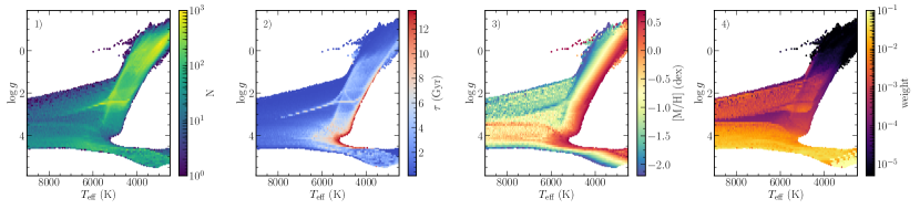
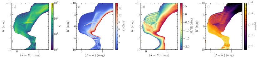
Figure 1: $T_{\rm eff}$ $vs$ $\log g$  (top) and $(J-K_{s})$ $vs$ $K_{s}$ (bottom) hexbin plots of the isochrones employed in this work to derive the ages, masses, and reddenings. Panels 1) are colour-coded by density of points, panels 2) by average age, panels 3) by average metallicity and panels 4) by average evolutionary weight (factor $\beta_{i}$ in Eq. 1).

We used the PARSEC stellar tracks (Bressan et al., 2012) version 1.2S (Tang et al., 2014; Chen et al., 2015) up to the beginning of Asymptotic Giant Branch (AGB) and the COLIBRI $S_{37}$ tracks up to the end of the AGB phase (Pastorelli et al., 2020; Marigo et al., 2013; Rosenfield et al., 2016), in combination with the online interpolator tool of the Padova group, to compute a library of isochrones spanning the ages between $0.1$ and $13.5\,{\rm Gyr}$, logarithmically spaced by a $\log(\tau)$ step of $0.05$, and the metallicities between $-2.2$ and $+0.7\,{\rm dex}$ with a step of $0.05\,{\rm dex}$ ($i.e.$ of the same order as GSP-Spec’s uncertainties on metallicity). The metallicity values for the isochrones are obtained using the approximation $\rm{[M/H]}=\log(Z/X)-\log(Z/X)_{\odot}$, with $(Z/X)_{\odot}=0.0207$ and $Y=0.2485+1.78Z$, and where $X,Y,Z$ are, respectively, the hydrogen, helium and metal abundances, by mass (Caffau et al., 2011; Basu & Antia, 1997).

In total, 2 301 different isochrone tracks, containing 842 494 tabulated $T_{\rm eff}$, $\log g$, [M/H], $\tau$, initial stellar mass ($M_{\rm ini}$), absolute magnitudes in the $G$, $G_{{BP}}$, $G_{{RP}}$ EGDR3 photometric bands and in the 2MASS $J$, $H$, $K_{s}$ bands were obtained in such a way. Their $T_{\rm eff}$ vs $\log g$ and $(J-K_{s})$ vs $K_{s}$ distribution and properties are shown in Fig. 1. This set of isochrones is the one that is going to be used in what follows in order to project the atmospheric parameters on.

2.2 Isochrone projection algorithm

The method described below was initially inspired by Zwitter et al. (2010) and early implementations of it have already been successfully employed for either distance computation (Kordopatis et al., 2011, 2013, 2015b; Recio-Blanco et al., 2014), age derivation (Kordopatis et al., 2016; Magrini et al., 2017, 2018; Santos-Peral et al., 2021) or reddening estimation (Schultheis et al., 2015; Zhao et al., 2021). For completeness, we summarise in what follows the method, which contains specific changes that have been implemented for the Gaia-RVS application.

We consider a star in the Gaia catalogue, to which is associated a set of observed parameters $\hat{\theta}_{k}$ ($k\equiv$ $T_{\rm eff}$, $\log g$, [M/H], $G$, $J$, $H$, $K_{s}$,…) and uncertainties $\sigma_{\hat{\theta}_{k}}$. The projection on the isochrones is performed as follows:

1. We select all of the isochrone points that have tabulated values within $n\cdot\sigma_{\hat{\theta}_{k}}$ from each considered observed parameter, where $n$ is arbitrarily chosen by the user. If less than 50 points are selected, the range is expanded to $3n\cdot\sigma_{\hat{\theta}_{k}}$. This usually happens when the observed uncertainties are largely under-evaluated.
   

2. For each selected node on the isochrones, $i$, we assign a Gaussian weight $w_{i}$, which depends primarily on its distance from the measured observables. In practice:

   $$w_{i}=p_{i}\cdot\beta_{i}\cdot\exp\left(-\sum_{k}\frac{(\theta_{i,k}-\hat{\theta}_{k})^{2}}{2\sigma_{\hat{\theta}_{k}}^{2}}\right),$$ (1)

   where $\theta_{i,k}$ corresponds to the tabulated parameters of the isochrones. The factor $\beta_{i}$, suggested by Zwitter et al. (2010), is defined as the stellar mass difference between two adjacent points on the same isochrone. It is equivalent to assuming a flat prior on stellar mass, and it provides higher probability to the likelihood of observing dwarfs, reflecting their slower evolutionary phases (see panel 4 of Fig. 1). The parameter $p_{i}$ is the prior on the age. It is equal to one if a flat prior is considered, or it can be a more complex function depending on the a priori knowledge of the investigated stellar population. The one adopted in this work is shown in Fig. 2, and is discussed in Sect. 2.3.
   

3. The projected parameters $\theta^{*}_{k}$, are obtained by computing the weighted mean of the selected set of tabulated stars with parameters $\theta_{k}$:

   $$\theta^{*}_{k}=\frac{\sum_{i}w_{i}\cdot\theta_{k,i}}{\sum_{i}w_{i}}.$$ (2)

4. Finally, the associated uncertainty is obtained by computing the weighted dispersion :

   $$\sigma_{\theta^{*}_{k}}=\sqrt{\frac{\sum_{i}w_{i}\cdot(\theta^{*}_{k}-\theta_{k,i})^{2}}{\sum_{i}w_{i}}}.$$ (3)

Because in practice the method computes as many weights $w_{i}$ as points on the isochrones, restricting the computation to the points within $4\cdot\sigma_{\hat{\theta}_{k}}$ from the measurements (Step 1, above) ensures a significant speed-up of the algorithm without losing any contribution from isochrone points that are far from the input data. In addition, Step 1 also ensures that no age, mass, etc is returned if the measured parameters are too far from the set of isochrones. This is particularly crucial for the very low metallicity stars ([M/H]$<-2.2$ dex), since a $T_{\rm eff}$-$\log g$ match could, in principle, be found, despite being far from the edge of the grid of isochrones.

Eventually, the algorithm returns as many parameters as the ones tabulated on the isochrones. We save, however, only the projected $T_{\rm eff}$, $\log g$ and [M/H], the age ($\tau$), the initial stellar mass ($M_{\rm ini}$), the absolute magnitudes $G$, $G_{{BP}}$, $G_{{RP}}$ and their associated uncertainties. From the projected magnitudes, one can also infer the interstellar reddening, $E(G_{BP}-G_{RP})$, and the interstellar extinction, $A_{G}$ (see Sect. 2.8).

We note that the difference between the input $T_{\rm eff}$, $\log g$ and [M/H] and the output (i.e. projected) ones can serve as diagnostics of the projection. Typically, when the difference is too large, this implies that no isochrones are found nearby the input values, therefore questioning the reliability of the output parameters (and perhaps the input ones as well).

2.3 Choice of an age prior

Unlike some isochrone projection methods available in the literature (some of them optimised to only get the line-of-sight distances, see Sect. 1), the one we present in this paper does not adopt a specific age prior based on the galactic populations (see Fig. 2). As a matter of fact, for the majority of the stars ($-0.7\leq\rm{[M/H]}\leq 0$ dex) a flat prior is adopted. This choice is motivated by the facts that the definitions of thin and thick discs are not as clear as they used to be (chemical vs geometrical discs, see for example Hayden et al., 2017), that Gaia-Enceladus-Sausage spatial and chemical distribution is complex and partly entangled with the disc (see for example Belokurov et al., 2018; Helmi et al., 2018; Myeong et al., 2019; Feuillet et al., 2020), and that the properties of many of the other accreted populations highlighted with Gaia show that a given locus in physical and chemical spaces is a mix of several different populations of different ages (e.g., Kordopatis et al., 2020; Laporte et al., 2020; Naidu et al., 2020; Gaia Collaboration, Antoja, T. et al., 2021, and references therein).

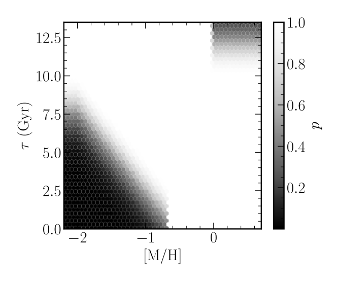
Figure 2: Age priors, $p$, adopted in this work, used in Eq. 1. These are half-Gaussians of $\sigma=2\,{\rm Gyr}$, centred on different ages depending on the metallicity.

Such a flat age prior, however, is poorly justified for super-solar metallicity or metal-poor stars, for which one can safely suppose that the former cannot be too old (metal-rich bulge stars are $\sim 9\,{\rm Gyr}$, e.g. Schultheis et al., 2017; Bovy et al., 2019) and that the latter cannot be too young (the metal-poorest thin disc stars in the Solar neighbourhood are found to be $\sim 8-9\,{\rm Gyr}$ old whereas the thick disc is found to be older than $7-8\,{\rm Gyr}$, see e.g. Bensby et al., 2014; Haywood et al., 2018). For this reason we adopt half-Gaussian weights, for $\tau>\tau_{c}$ if $\rm{[M/H]}>0$ or $\tau<\tau_{c}$ if $\rm{[M/H]}<-0.7\,{\rm dex}$:

$$p=\exp\left(-\frac{(\tau-\tau_{c})^{2}}{2\cdot\sigma_{\tau}^{2}}\right).$$ (4)

We take $\tau_{c}=10\,{\rm Gyr}$ for $\rm{[M/H]}>0\,{\rm dex}$ and $\rm{[M/H]}<-2\,{\rm dex}$, i.e. a star has less probabilities of being older than $10\,{\rm Gyr}$ if it has a super-solar metallicity and less probabilities of being younger than $10\,{\rm Gyr}$ if it is more metal-poor than $-2\,{\rm dex}$. For stars with $-2<\rm{[M/H]}<-0.7\,{\rm dex}$, we adopt:

$$\tau_{c}=-5.4\cdot\rm{[M/H]}-0.8,$$ (5)

which imposes $\tau_{c}=3\,{\rm Gyr}$ at $\rm{[M/H]}=-0.7\,{\rm dex}$ and $\tau_{c}=10\,{\rm Gyr}$ at $\rm{[M/H]}=-2\,{\rm dex}$. The resulting weights as a function of metallicity are shown in Fig. 2.

2.4 Validation of the method on synthetic data

In order to evaluate the method’s performance, we first test it on a set of synthetic data. We randomly select, amongst the entire isochrone set (Sect. 2.1), 200 turn-off stars (defined as $5000\leq$ $T_{\rm eff}$$\leq 8500$ K and $\log g$$\geq 3.5$), 200 Red Giant Branch (RGB) stars (defined as $T_{\rm eff}$$\leq 6000$ K and $\log g$$<3.5$) and 200 main-sequence stars (defined as $T_{\rm eff}$$<4800$ K and $\log g$$\geq 4.0$). We note that this sample contains non-realistic stars, e.g. metal-rich stars older than 12 Gyr. We make sure, however, not to select stars younger than 5 Gyr  with metallicities lower than $-1$ dex.

We consider four different types of projection, labelled as follows:

• spec: projects only $\hat{\theta}_{k}=${$T_{\rm eff}$, $\log g$, [M/H]}.

• speck: projects {$T_{\rm eff}$, $\log g$, [M/H], $K_{s}$}.

• specjhk: projects {$T_{\rm eff}$, $\log g$, [M/H], $J$, $H$, $K_{s}$}.

• specjhkg: projects {$T_{\rm eff}$, $\log g$, [M/H] $J$, $H$, $K_{s}$, $G$}.

In addition, we consider different test-cases, where the value of each of the input parameters is randomised according to a normal distribution of standard deviation associated to a given uncertainty (see Table 1). The sample labelled ‘Q25’ adopts the parameter uncertainties of the 25th percentile of the GSP-Spec  catalogue for a given specific parameter. Similarly, Q50 and Q95 adopt the uncertainties of the 50th and 95th percentiles. We note that the uncertainties for the photometric filters are estimated as the quadratic sum of the uncertainty of the apparent magnitude in that filter and the uncertainty on the absolute magnitude derived by the distance modulus (see Sect. 2.6.1 for further details).

Table 1: Uncertainty percentiles for the GSP-Spec sample adopted for the performance tests of the projection method.

parameter	Q25	Q50	Q75	Q95
$T_{\rm eff}$ (K)	35	70	130	350
$\log g$ ($g$ in  $\rm cm\leavevmode\nobreak\ s^{-2}$)	0.1	0.2	0.35	0.5
[M/H] (dex)	0.05	0.1	0.2	0.4
$G$ (mag)	0.015	0.03	0.06	0.14
$J$, $H$, $K_{s}$ (mag)	0.03	0.04	0.07	0.15

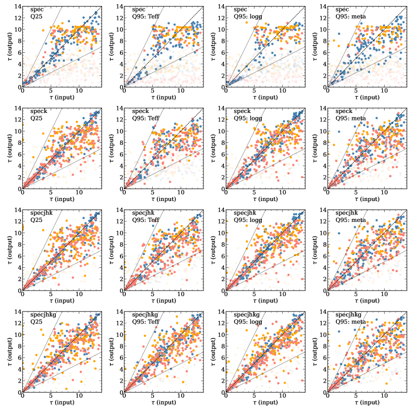
Figure 3: True versus output ages (in Gyr) for the test sample of synthetic data. Blue, orange and red points represent turn-off, main-sequence and red giant stars, respectively. The dashed black line represents the 1:1 relation, on which a star with perfectly well estimated age should be on. Dotted lines show deviations from perfect estimation of $\pm 50$ per cent. Input parameters are randomised according to the Q25 uncertainties (see Table 1), unless specified at the top left corner. First row plots consider a projection of only $T_{\rm eff}$, $\log g$ and [M/H]  (labelled spec), whereas rows two, up to four consider in addition the $K_{s}$ magnitude (speck), the $J,H,K_{s}$ magnitudes (specjhk), and the $J,H,K_{s},G$ magnitudes (specjhkg), respectively. Finally, solid points are the stars for which the estimated relative age uncertainty is smaller than 50 per cent, whereas the semi-transparent ones have estimated relative age uncertainties larger than 50 per cent. See Sec. 2.4 for further details.

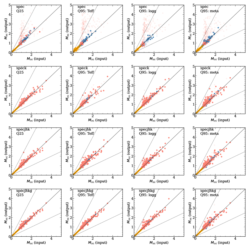
Figure 4: Same as Fig. 3 for the initial stellar masses. Semi-transparent points are the ones having estimated relative age uncertainties greater than 50 per cent, whereas the filled circles have estimated age uncertainties smaller than 50 per cent.

Figures 3 and 4 compare the real and the derived ages and masses, where each row shows a different projection flavour. Q25 uncertainties are adopted for all of the parameters, except for columns two to four, where one parameter each time adopts Q95, as indicated at the top left corner (while keeping the other parameters at Q25). Solid circles are the stars for which the estimated relative uncertainty in age is smaller than 50 per cent, whereas the semi-transparent circles have uncertainties larger than 50 per cent.

These figures show that, provided we apply a 50 per cent filter on the estimated relative age uncertainty, the ages for turn-off stars are always well determined (blue points), even when input parameter uncertainties are large (Q95). On the other hand, giants and main-sequence stars (red and orange points, respectively) require additional information to be used during the projection (which can be in the form of absolute magnitudes or age priors) in order to have their ages well derived. When this is done, speck, specjhk and specjhkg return reliable estimations (age errors smaller than 50 per cent) for all of the stellar types, even with Q95 input uncertainties.

The mass estimations for main-sequence and turn-off stars are always reliable, regardless of the projection-flavour or input parameter uncertainties. This is not the case for giants, for which the spec projection overestimates the values. Furthermore, we find that the mass uncertainties are generally underestimated, and that a filtering on the age uncertainty removes more efficiently the outliers, at the cost of removing simultaneously the mass estimations for the main-sequence stars. In what follows, we decide to filter-out the masses of solely the giants only if their relative age uncertainty is larger than 50 per cent.

Finally, we also investigated the effect of magnitude uncertainties, as well as interstellar reddening on the output parameters. For this test-case we set uncertainties for $T_{\rm eff}$, $\log g$  and [M/H]  always equal to Q50, whereas we adopted uncertainties for $J$, $H$, $K_{s}$ and $G$ of Q25 and Q95. Three different extinction values were considered: $A_{V}=0.0$ mag , $A_{V}=0.2$ mag and $A_{V}=2.5$ mag (converted for each filter, see Sect. 2.6.2). Results for the ages are shown in the Appendix B. In short, speck projection always gives good ages and masses, even with Q95 and $A_{V}=2.5$ mag. We find that $A_{V}=0.3$ introduces small biases for specjhk and specjhkg if the uncertainties on the magnitudes are small (i.e. Q25), but this bias mostly disappears for larger uncertainties (Q95).

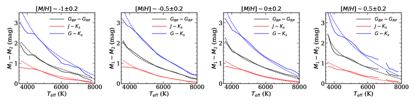
Figure 5: Relation between $T_{\rm eff}$  and $G_{{BP}}$$-$$G_{{RP}}$ (black), $J-K_{s}$ (red), $G-K_{s}$ (blue) for the adopted isochrones (in dashed lines), and the Gaia-RVS observed stars (solid lines) within 150 pc from the Sun (to minimise the extinction effects) at four different metallicity regimes.

2.5 Specific considerations for projection of real data

When projecting real Gaia data on the isochrones, some specific points, that were not considered in the previous sections, need to be taken into account. These, concern the colour-calibration of the isochrones, and the $\alpha-$ enhancement of the stars. We discuss these points below.

2.5.1 Colour-$T_{\rm eff}$ calibration

For a reliable projection on the isochrones (or if one desires to use the output $G_{{BP}}$  and $G_{{RP}}$ magnitudes, see Sect. 2.8), the relation between the $T_{\rm eff}$ and the colour indexes must be the same for the observed values (in our case, GSP-Spec) and for the ones on the isochrones. Following Santos-Peral et al. (2021), we investigated the relation between these two, for four different metallicity regimes ($-1,-0.5,0,+0.5\,{\rm dex}$) for stars closer than 150 pc from the Sun, in order to minimise the effect of reddening on the observed colours. Results shown in Fig. 5 suggest no significant differences between the isochrone and the observed relations, at least for stars hotter than 4000 K, therefore implying that no specific calibration needs to be performed on the isochrone colours in order to be on the same scale as GSP-Spec’s $T_{\rm eff}$.

2.5.2 Effect of non-solar $\alpha$-enhancement

PARSEC isochrones do not include any variation of $\alpha-$abundance. Indeed, all of the sets adopt solar value. In order to evaluate the effect of non-solar $\alpha$-enhancement, we used the Salaris et al. (1993) formula, as derived in Valentini et al. (2019), to convert GSP-Spec’s calibrated [M/H]  to a proxy for the overall metallicity including $\alpha-$elements, $\rm{[M/H]}_{\alpha}$. The adopted formula, is the following:

$$\rm{[M/H]}_{\alpha}=\rm{[M/H]}_{GSP-Spec}+\log_{10}(C\cdot 10^{\rm[\alpha/Fe]}+(1-C))$$ (6)

with C$=0.661$, and with $\rm[\alpha/Fe]$ the calibrated value provided by GSP-Spec obtained with a third degree polynomial (see first row of Table 4 of Recio-Blanco et al. 2022).

Using the spec projection, adopting one or the other metallicity estimate, resulted to differences smaller than $1\,{\rm Gyr}$ and $0.1M_{\odot}$ for 90 per cent of the stars, for $\tau$ and $\rm{M_{ini}}$, respectively.

Given that these differences are smaller than the uncertainty on the derived ages and masses, and to the fact that $\rm[\alpha/Fe]$ abundances have a precision of the order of $\sim 0.07$ dex (that can become larger depending on the quality of the spectra, see Recio-Blanco et al. 2022), we decided in what follows not to use $\rm{[M/H]}_{\alpha}$ . However, projections obtained using $\rm{[M/H]}_{\alpha}$ can be provided, upon request to the first author.

2.6 Gaia DR3 application: Computation of the datasets

2.6.1 Projection flavours, input parameters and associated uncertainties

We performed four different isochrone projections (leading therefore to four sets of ages, masses, interstellar extinctions), according to the flavours described in Sect. 2.4: spec, speck, specjhk and specjhkg.

The atmospheric parameters are the calibrated GSP-Spec  ones, following Eq. 1 (for $\log g$) and Eq. 2 (for [M/H], with a fourth degree polynomial) of Recio-Blanco et al. (2022). The absolute magnitudes in the $G$, $J$, $H$ and $K_{s}$ bands have been obtained using the distance modulus, adopting the Bailer-Jones et al. (2021) geometric distances ($r$) that assume a distance prior along with the parallax information, and neglecting entirely the line-of-sight extinction. Although this assumption has no consequence for the spec projection, neglecting the line-of-sight extinction introduces an increasing amount of bias in the output ages and masses the bluer the central wavelength of the filter (i.e. in increasing order: $K_{s}$, $H$, $J$ and lastly $G$, see Appendix B).

The uncertainties required in Eq. 1 for the projection, are obtained assuming Gaussian posteriors for GSP-Spec $T_{\rm eff}$, $\log g$ and [M/H] (i.e. taking half of the difference between the upper and lower confidence value). The uncertainty on the absolute magnitudes $M_{\lambda}$, for a given filter $\lambda$, are obtained as the quadratic sum of the uncertainty on the observed magnitude, $m_{\lambda}$, and the uncertainty term coming from the distance modulus $\mu$:

$$\sigma_{M_{\lambda}}=\sqrt{\sigma^{2}_{\mu}+\sigma^{2}_{m_{\lambda}}},$$ (7)

where $\sigma_{\mu}$ is the uncertainty on the distance modulus derived using standard error analysis:

$$\sigma_{\mu}=\frac{\sigma_{r}}{0.461\cdot r},$$ (8)

with $\sigma_{r}$ the (assumed) Gaussian uncertainty on the distance ($r$), obtained also as the half of the difference between the upper and the lower confidence value of $r$.

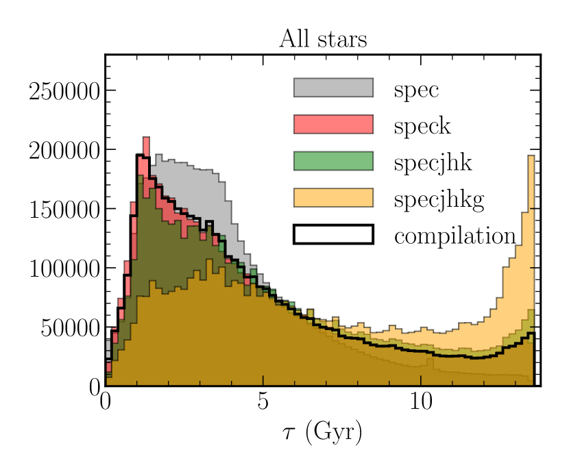
Figure 6: Histograms of age (top) and initial mass (bottom, in logarithmic scale) of each projection flavour and for the compiled sample, for all the GSP-Spec stars that have a KMgiantPar_flag $=0$.

Figure 6 compares the age (top) and mass (bottom) distributions of the different projections. Each distribution contains all of GSP-Spec’s stars, except those having KMgiantPar_flag $\neq 0$, for which $T_{\rm eff}$ and $\log g$ are less reliable (see Recio-Blanco et al., 2022). One can see that the specjhkg projection finds significantly older stars, especially compared to the spec projection, the latter showing the youngest ages, on average, with a broad peak at $\tau\sim 3.5\,{\rm Gyr}$. These differences can be understood given the analyses in the previous sections; on the one hand, as extinction is not taken into account in the speck, specjhk and specjhkg projections, giants with reddened colours tend to lie on older isochrones, biasing the age estimation towards larger values. As shown in Appendix B, this bias is stronger the bluer the filter, eventually leading to the peak at $\tau\sim 12\,{\rm Gyr}$ for the specjhkg projection. On the other hand, the spectroscopic projection, as shown in Fig. 3, tends to be biased towards younger ages for all stellar types except the turn-off stars.

2.6.2 Catalogue compilation

The differences seen in Fig. 6, naturally lead to the necessity of finding an optimal combination of projection flavour in order to get the most reliable ages and masses.

This was attempted by obtaining the dust-reddening $E(B-V)$ maps from Schlegel et al. (1998), using the Python script dustmaps (Green, 2018), and correcting the most reddened regions ($E(B-V)>0.1$) as in Bonifacio et al. (2000). These were then converted into $A_{V}$, assuming $R_{V}=3.1$, and then to $A_{J}$, $A_{H}$, $A_{Ks}$ and $A_{G}$, following the adopted PARSEC 3.5 extinction coefficients of Cardelli et al. (1989), O’Donnell (1994) and the Gaia EDR3 passbands of Riello et al. (2021), as summarised in Table 2. Finally, these extinctions were then compared with the uncertainties of the absolute magnitudes in each respective band, as derived from Eq. 7.

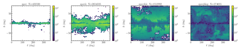
Figure 7: Spatial distribution, in galactic sky-coordinates $(\ell,b)$, of the number of stars for which we adopt each projection flavour. The total of selected stars and the considered projection are indicated at the top of each plot. Only targets with GSP-Spec KMgiantPar_flag$=0$ are considered here.

Table 2: Extinction conversions, as adopted from PARSEC 3.5.

	$A_{J}$	$A_{H}$	$A_{Ks}$	$A_{G}$
$A_{\lambda}/A_{V}$	0.28665	0.18082	0.11675	0.83278

To compile our final, adopted, catalogue (labelled without any underscore in Table 3), we selected, for a given star, the projection flavour according to the scheme below:

• speck where $A_{Ks}\leq\sigma_{M_{Ks}}$, or $r\leq 300$ pc and $A_{V}\leq 3$ mag.

• specjhk where $A_{J}\leq\sigma_{M_{J}}$, or $r\leq 100$ pc.

• specjhkg where $A_{G}\leq\sigma_{M_{G}}$, or $r\leq 50$ pc.

• spec otherwise.

The resulting age and mass distributions of the compiled sample are shown in black in Fig. 6. The conditions regarding the distance and $A_{V}$ are empirical, and take into account the fact that Schlegel’s values are the total extinctions along the line-of-sight, and that the Sun resides within a local bubble with very little extinction (Fitzgerald, 1968; Lallement et al., 2014). The extinction criterion is an educated guess resulting from the analysis of Sect. 2.4 using reddened projections of synthetic data. Figure 7 shows the number of stars in bins of galactic $(\ell,b)$ where each projection flavour is adopted. The spec flavour is, as expected, selected only for stars within the galactic plane, and the speck flavour is the one that contains the most of the stars. Finally, the specjhkg flavour contains the smaller number of stars, spread, however, all over $(\ell,b)$.

Figure 8: $T_{\rm eff}$-$\log g$ diagrams adopting GSP-Spec parameters (top) and isochrone-projected parameters (bottom). Colour-code represents GSP-Spec calibrated metallicity, age (in Gyr) and initial stellar mass (in $M_{\odot}$). Only targets with first 12 quality GSP-Spec flags $\leq 1$ and KMgiantPar_flag$=0$ are considered here.

Figure 8 shows Kiel diagrams colour-coded by either metallicity, age or initial mass, with the input $T_{\rm eff}$ and $\log g$ (top row), and the output ones (bottom row). These plots show that the parameters we recover in different regions of the diagram are compatible with what one would expect: low mass stars are mainly cool dwarfs, and old stars are at the redder part of the RGB. Similarly, the turn-off region contains significantly younger stars.

To conclude, we note that in the published catalogue (see Table 3), the parameters resulting from this compilation are labelled without underscores. For the users that wish to perform their own combination of flavours, based on different criteria than the ones adopted here, the results from each separate flavour are also published, with the appropriate and explicit label-name.

2.7 Validation of the ages and masses

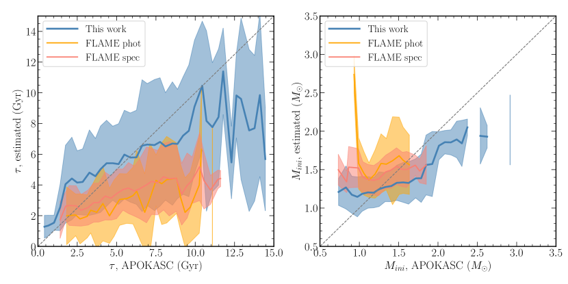
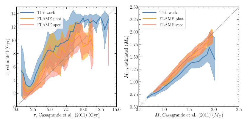
Figure 9: Comparison of the derived ages (left) and masses (right) with the APOKASC-2 (top) and Casagrande et al. (2011) (bottom) catalogues. Plots show running medians in bins of reference (catalogue) values. In blue are shown the values derived with the compiled catalogue of Sect. 2.6.2. In red and orange are shown the results of the FLAME-Spec and FLAME-Phot modules, respectively. Shaded areas represent the $\pm 1\sigma$ around the running medians. Only the targets that have GSP-Spec flags equal to zero and relative age uncertainties (on each module separately) smaller than 50 per cent are selected. Additional cuts, imposing $\rm{[M/H]}>-0.5\,{\rm dex}$, are applied for the FLAME results.

To validate our ages and masses we compare our results with the APOKASC-2 asteroseismic values (Pinsonneault et al., 2018) that include a wide metallicity range ($-2.5\leq\rm{[M/H]}\leq 0.5$ dex) but concern only giants ($\log g$$<3.3$), and the values from Casagrande et al. (2011) that concern mostly main-sequence stars. We also compare the mean ages we derive for open clusters with the ones of Cantat-Gaudin et al. (2020) and perform a similar exercise for globular cluster based on the selection of Gaia Collaboration et al. (2018). Finally, we compare the values we obtain with the ones of the FLAME pipeline for the entire sample. In the subsections that follow, we always remove the stars that have a Renormalised Unit Weight Error (RUWE) greater than 1.4, as they could potentially be non-single sources (see Lindegren, 2018), as well as the stars with GSP-Spec KMgiantPar_flag$>0$.

2.7.1 Comparison with APOKASC-2 and Casagrande et al. (2011) ages and masses

We required the 12 first GSP-Spec  parameter quality flags to be smaller or equal to one (i.e. very good quality sample with the small atmospheric parameter uncertainties) and selected stars with relative output age uncertainties smaller than 50 per cent. The mean offset and standard deviations between the GSP-Spec  atmospheric parameters and the literature ones are, for $T_{\rm eff}$, $\log g$ and [M/H]: $-20\pm 100\,K$, $0.01\pm 0.21\,{\rm dex}$, $-0.11\pm 0.09\,{\rm dex}$ for the APOKASC-2 sample, and $-74\pm 132\,K$, $-0.06\pm 0.17\,{\rm dex}$, $-0.17\pm 0.13\,{\rm dex}$ for the Casagrande et al. (2011) sample.

The blue lines in Fig. 9 show the running median in bins of reference catalogue values (i.e. APOKASC-2 or Casagrande et al. 2011), for the compiled sample as defined in Sect. 2.6.2. For comparison purposes, running medians obtained when considering the FLAME-Spec and FLAME-Phot datasets are also shown in red and orange.

One can see that we manage to reproduce adequately the literature ages, with mean offsets and standard deviations between the literature and the derived values of $(-0.77\pm 3.4)\,{\rm Gyr}$ for APOKASC-2 and $(-2.4\pm 2.6)\,{\rm Gyr}$ for Casagrande et al. (2011). These values drop to $(0.2\pm 2.3)\,{\rm Gyr}$ and $(-1.5\pm 2.3)\,{\rm Gyr}$ when we impose differences between the GSP-Spec atmospheric parameters and the literature ones smaller than $150\,K,0.15\,{\rm dex}$ and $0.1\,{\rm dex}$ for $T_{\rm eff}$, $\log g$ and [M/H], respectively.

We find that the ages for the giants tend to be slightly over-estimated until $\tau\sim 11\,{\rm Gyr}$, above which value the median trend shows an underestimation of the ages. The first reason for this is that ages for old giants are inherently difficult to determine accurately because the isochrones are close to each other. Furthermore, since we do not have isochrones older than 13.7 Gyr, our code tends to sample asymmetrically the ages, leading to a larger selection of young isochrones compared to old ones. Additionally, we note that we have a relatively large disagreement on the ages of the youngest stars of Casagrande et al. (2011). Whereas it is not clear what is the origin of this large disparity, one can see that we also find a similar trend with FLAME-Spec and FLAME-Phot parameters, the later being based on completely different input parameters.

As far as the masses are concerned, we find a very good agreement, both for APOKASC-2 and Casagrande et al. (2011), with a slight overestimation of the masses for sub-solar mass giants, and a slight under-estimation for stars with masses greater than $\sim 1.5\,M_{\odot}$. The mean offsets and standard deviations between the literature and the derived values are of $(0.00\pm 0.3)\,M_{\odot}$ for APOKASC-2 and $(0.1\pm 0.1)\,M_{\odot}$ for Casagrande et al. (2011). These values become $(-0.1\pm 0.2)\,M_{\odot}$ and $(0.09\pm 0.08)\,M_{\odot}$ when we impose differences between the GSP-Spec atmospheric parameters and the literature ones smaller than $150\,K,0.15\,{\rm dex}$ and $0.1\,{\rm dex}$ for $T_{\rm eff}$, $\log g$ and [M/H], respectively.

2.7.2 Open cluster ages

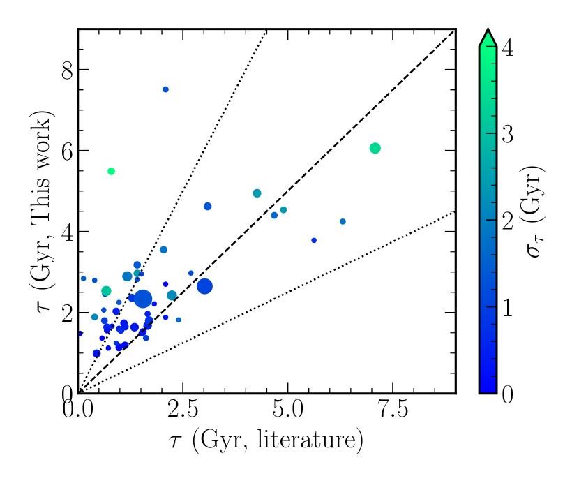
Figure 10: Comparison of median open cluster ages with the ones of Cantat-Gaudin et al. (2020). The colour-code corresponds to the age dispersion that we obtain within the cluster, and the size of the points is proportional to the number of cluster members that made our selection. A minimum of three stars per cluster has been imposed. Dashed diagonal line represents the 1:1 relation, whereas the dotted lines show deviations from identity of $\pm 50$ per cent.

We selected from the sample of Cantat-Gaudin et al. (2020) the stars that have a published probability higher than 95 per cent of being part of a considered open cluster. We furthermore filtered out the stars that have GSP-Spec flags greater than 1 and output relative age uncertainties greater than 50 per cent. From the resulting sample we computed the mean ages and dispersion per cluster and compared these numbers to the values published by Cantat-Gaudin et al. (2020). Results are shown in Fig. 10. They suggest we perform very well for the young targets, with a small overestimation of the ages by $0.6\,{\rm Gyr}$ and an inner cluster age dispersion of the order of $\sim 1\,{\rm Gyr}$ for most of the objects that contain at least some turn-off or subgiant stars.

Amongst the few clusters for which the disagreement with the literature values is greater than 50 per cent (dashed lines in Fig. 10), we can identify two different cases. On the one hand, we have the clusters that contain mostly main-sequence stars, known to constrain poorly the age (see the case of Melotte25 in Fig. 24). On the other hand, we have the objects for which we suspect that the input parameters could be slightly biased, since our proposed solution fits better the observed parameters than the isochrone with the literature age. These biases can either be due to a metallicity calibration that is different than for field stars (see Fig. 13 of Recio-Blanco et al., 2022) or due to large uncertainties on the distance modulus. The open cluster NGC2112 likely falls into this category, with a discrepancy with the literature estimations of $\sim 5\,{\rm Gyr}$ (Carraro et al., 2002; Kharchenko et al., 2013; Cantat-Gaudin et al., 2020).

2.7.3 Globular cluster ages

We investigated the performance of our code for old and metal-poor stars, i.e. stars belonging to globular clusters. This regime is known to be difficult to get ages for field stars, as the isochrones, especially for giants are very close one to another. We selected the globular cluster targets compiled in Gaia Collaboration et al. (2018) and cross-matched them with our sample, requiring GSP-Spec quality flags on the atmospheric parameters to be less than or equal to 1. Furthermore, the median S/N of the selected spectra being low, of the order of $30$, we required that the differences between the input and output $T_{\rm eff}$, $\log g$ and [M/H] to be less than 200 K, 0.3 and 0.1 dex, in order to ensure that we have measurements close to the isochrones. For the six globular clusters that contained at least three stars fulfilling the conditions above, we computed the mean age, with the expectation of finding them older than $10\,{\rm Gyr}$ (e.g. VandenBerg et al., 2013).

Despite the adopted age-prior for the metal-poor stars, we find ages ranging between $3.5\,{\rm Gyr}$ and $9.3\,{\rm Gyr}$, consistent with the results of Sect. 2.7.1 for APOKASC-2, that suggest that old targets tend to have under-estimated ages. A closer investigation of the Kiel and $T_{\rm eff}$-$M_{K_{s}}$ diagrams (see Fig. 25) highlights the difficulty of determining these ages properly due to the proximity of the various isochrones. On top of this challenge, we find that the mean metallicity of the stars within each cluster tend to differ by $\sim+0.15\,{\rm dex}$ compared to, for example, the values reported by VandenBerg et al. (2013). This metallicity difference, also noted in Gaia Collaboration, Recio-Blanco et al. (2022), without, however suggesting a specific calibration for these objects, is also partially responsible for the age offsets we find, compared to expectations.

2.7.4 Comparison with FLAME ages and masses

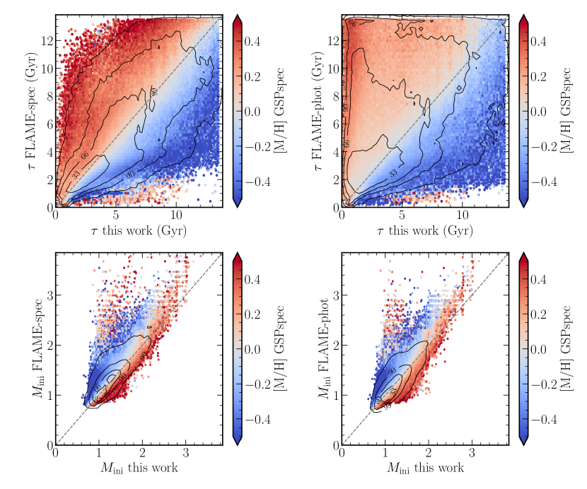
Figure 11: Comparison of the ages (top) and the masses (bottom) between the estimations obtained in this work and with the ones of FLAME-Spec (left) and FLAME-Phot (right). Only GSP-Spec turn-off stars with all the first 13 GSP-Spec flags equal to zero are selected here, with age uncertainties (both in our code and the FLAME modules) smaller than 50 per cent. Contour lines contain 33, 66, 90 and 99 per cent of the distribution. The colour code is GSP-Spec’s calibrated [M/H].

Figure 11 compares our ages and masses with the ones derived from FLAME, obtained either with GSP-Phot input (i.e. FLAME-Phot) or with uncalibrated GSP-Spec (i.e. FLAME-Spec). We recall that our ages and masses, regardless if photometry is taken into account or not, are always estimated with the GSP-Spec $T_{\rm eff}$, and the calibrated GSP-Spec $\log g$, and [M/H]. To obtain this plot, only turn-off stars are selected (based on calibrated GSP-Spec parameters), since FLAME results are less reliable for the giants (see Creevey et al., 2022; Fouesneau et al., 2022). We also imposed GSP-Spec  parameter flags smaller or equal to 1 and relative age uncertainties (based on the different age estimations) smaller than 50 per cent.

The agreement of FLAME with our ages and masses can be considered as adequate only for metallicities close to solar values. Figure 11 shows that as soon as [M/H] is different than zero, then the disagreement becomes non negligible. Indeed, for stars with $\rm{[M/H]}=\pm 0.15\,{\rm dex}$, we find mean age offsets of $0.09\pm 1.29\,{\rm Gyr}$ and $-0.01\pm 1.40\,{\rm Gyr}$ compared to FLAME-Spec and FLAME-Phot, respectively. These values increase to $1.68\pm 1.60\,{\rm Gyr}$ and $1.63\pm 1.76\,{\rm Gyr}$ when considering stars with $\rm{[M/H]}<-0.15\,{\rm dex}$ and $2.96\pm 1.82\,{\rm Gyr}$ and $2.96\pm 1.89\,{\rm Gyr}$ for stars with $\rm{[M/H]}<-0.5\,{\rm dex}$. We therefore constrain the statement found in Fouesneau et al. (2022) that suggest to treat with caution FLAME ages for stars with [M/H]$\leq-0.5\,{\rm dex}$, to an even narrower metallicity range of $\pm 0.15\,{\rm dex}$ around solar values.

2.8 Calculation of the reddening and the extinction

To derive the extinctions, one must first compute the reddening $E(G_{BP}-G_{RP})$, obtained by measuring the difference between the projected and the observed colours ($G_{{BP}}$$-$$G_{{RP}}$). Extinction, $A_{G}$, is then computed using:

$$A_{G}=c_{\theta}\cdot E(G_{BP}-G_{RP}),$$ (9)

where $c_{\theta}$ is a constant that depends on the stellar type (Creevey et al., 2022; Fouesneau et al., 2022).

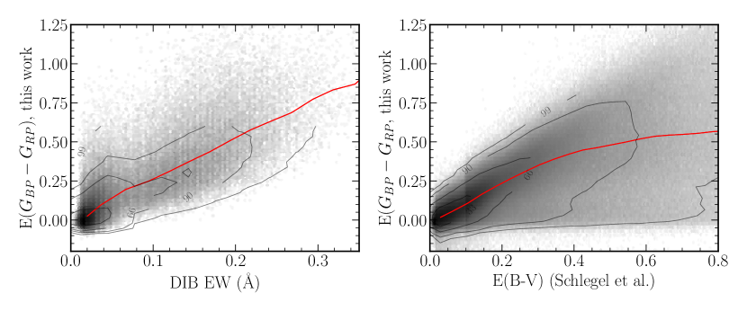
Figure 12: Comparison of $E(G_{BP}-G_{RP})$ derived in this work, with the equivalent widths of Diffuse interstellar bands at 862 nm derived from the same GSP-Spec spectra (left) and the Schlegel et al. (1998) $E(B-V)$ with the Bonifacio et al. (2000) correction (right). For both plots, the grey colour-scale is the logarithm of the number of stars in one bin, and the red lines represent the running median. The correlations are, in both cases, overall very good.

Left plot of Fig. 12 compares the reddening $E(G_{BP}-G_{RP})$ derived in our work, with the equivalent widths of the diffuse interstellar band at $\sim 862$ nm, as derived in Gaia Collaboration, Schultheis et al. (2022). The right plot compares with the Schlegel et al. (1998) $E(B-V)$ reddening (corrected as described in Sect. 2.6.2 towards the regions with the largest extinction). Overall, a good correlation is found with both dust proxies, confirming our estimations of reddening. We note, however, that some of our targets have $E(G_{BP}-G_{RP})$ values lower than zero. We decide not to artificially put them equal to zero, but draw the attention that the associated uncertainties of these stars should be considered.

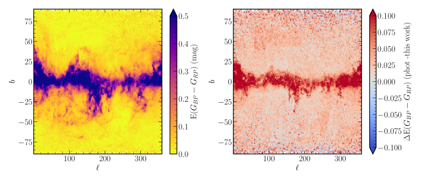
Figure 13: Left: $E(G_{BP}-G_{RP})$ distribution in galactic $(\ell,b)$ coordinates. Right: Residuals between the $E(G_{BP}-G_{RP})$ estimation from GSP-Phot and ours.

Left plot of Fig. 13 shows the reddening map derived for the sample. The right plot of the same Fig. shows the residuals between GSP-Phot’s $E(G_{BP}-G_{RP})$ values and ours. The median difference above and below galactic latitudes of $|b|=20^{\circ}$ is 0.019 mag and 0.052 mag, respectively. The agreement is rather good, acknowledging that GSP-Phot  does not use the same input data or parameters than we do, and that it is precisely towards highly reddened regions that degeneracies between $E(BP-RP)$ and $T_{\rm eff}$ make the GSP-Phot  parameterisation challenging.

2.9 Absolute magnitudes and line-of-sight distances

Finally, to validate more thoroughly the projected absolute magnitudes, we compare the geometric line-of-sight distances, $r$, of Bailer-Jones et al. (2021) with the ones derived via the distance modulus (correcting for the projected extinctions, assuming $c_{\theta}=1.83037$, valid for solar-type stars $\pm 1500\,K$). Results are shown in Fig. 14 (left: before correcting for the extinction, right: after applying the correction). They suggest that we find a very good agreement between the two distance estimations, with a null median residual and a dispersion of 20 pc. We find that the 1 per cent of stars that have the largest disagreement with the Bailer-Jones et al. (2021) distances have also either large differences between the input $\log g$  and the projected one ($>0.3$) if these stars are dwarfs, or large age uncertainties (larger than 50 per cent) if these stars are giants.

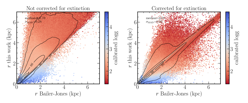
Figure 14: Comparison of the line-of-sight distances derived from the projected $M_{G}$ and extinction, with the geometric ones from Bailer-Jones et al. (2021). No cuts in the uncertainties on the Bailer-Jones et al. (2021) distances or in our line-of-sight distances are made.

Finally, we note that the very good agreement that is found is not necessarily a direct consequence of the use of $r$ when projecting the absolute magnitudes. Indeed, we recall that when we project the absolute magnitudes, extinction is ignored. As it can be seen on the left plot of this Figure (that does not correct for the derived interstellar reddening), when the estimated $A_{G}$ is neglected when computing the distance, the agreement between the two distance estimates is rather poor and biased.

3 Age and mass correlations with the orbital parameters and the positions in the Galaxy

In this section we illustrate the quality and the limitations of our projected parameters. To do so, we first compute the orbital parameters for all of the stars with measured radial velocities from the RVS and available astrometry. Then, we correlate them with the stellar ages and masses for a high-quality GSP-Spec sample, requiring the first 12 quality flags of GSP-Spec to be smaller or equal to one (except fluxNoise_flag that we require to be smaller or equal to 2), the KMgiantPar_flag that we require equal to zero, and the relative age uncertainty that we require to be smaller than 50 per cent.

3.1 Determination of Galactocentric positions, velocities and orbital parameters

The Galactocentric positions $X,Y,Z$ (in cartesian coordinates), $R$ (Galactocentric cylindrical radius), and cylindrical velocities (radial $V_{R}$, azimuthal $V_{\phi}$, vertical $V_{Z}$) in a right-handed frame have been computed for all of the stars that have a Gaia radial velocity measured ($\sim 33$ million targets). In order to do so, we used the star’s right ascension, declination, line-of-sight velocity, proper motions and Bailer-Jones et al. (2021) EGDR3 geometric and photogeometric Bayesian line-of-sight distances (therefore leading to two sets of positions, velocities and orbits). The assumed Solar position is $(R,Z)_{\odot}=(8.249,0.0208)$ kpc (Gravity Collaboration et al., 2020; Bennett & Bovy, 2019) and velocities $(V_{R},V_{\phi},V_{Z})_{\odot}=(-9.5,250.7,8.56)\,{\rm km\leavevmode\nobreak\ s^{-1}}$ (Reid & Brunthaler, 2020; Gravity Collaboration et al., 2020).

To compute the orbital parameters (actions, eccentricities, apocentre, pericentre, maximum distance from the Galactic plane), we used the Stäckel fudge method (Binney, 2012; Sanders & Binney, 2016; Mackereth & Bovy, 2018) with the Galpy code (Bovy, 2015), in combination with the axisymmetric potential of McMillan (2017) (adjusted to our adopted solar position and Local Standard of rest’s velocity). The lower and upper confidence limits (corresponding to the 16th and the 84th percentile) were obtained by propagating the uncertainties of the line-of-sight distance, line-of-sight velocity, and proper motions using 20 Monte-Carlo realisations. No correlation between proper motions and distance uncertainties were taken into account, and we assumed a non-gaussian distribution for $r$, constructed as two half-Gaussians defined by the upper and lower confidence limits of $r$.

3.2 Galactic maps of ages and masses and identification of the spiral arms

Maps of the stellar ages and masses in Galactic Aitoff projection $(\ell,b)$ are shown in Fig. 15. Young and massive stars are predominantly found in (or close to) the Galactic plane, within the regions of high reddening (see Fig. 13), as expected from the interstellar medium distribution in the Milky Way (e.g. Kalberla & Kerp, 2009, and references therein).

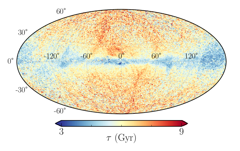
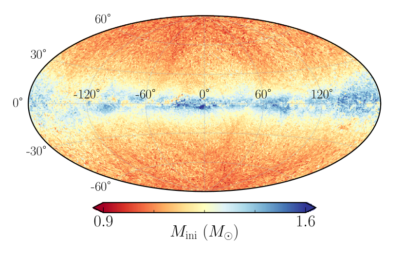
Figure 15: Healpix projections (NSIDE=64) of the mean ages (top) and masses (bottom) for the compiled sample.

In Fig. 16 we plot the Galactocentric cartesian X-Y positions of stars that have an estimated initial mass greater than 4 solar masses, $\log g$$<2$ (to avoid massive main sequence stars at the solar vicinity) and a maximum distance from the galactic plane during their orbit (i.e. $Z_{\rm max}$) less than 0.5 kpc. Superimposed, we also plot the position of the Perseus, Local, Sagittarius and Scutum spiral arms, based on Castro-Ginard et al. (2021) analysis of open clusters with Gaia EDR3 data (adapted to match our assumed solar position). The massive stars position follow very closely the one of the modelled spiral arms, consistent with the fact that the latter are regions where star formation takes place. Furthermore, one can also see the clear metallicity gradient within those stars, reflecting the metallicity of the interstellar medium at these locations (as these stars are found to be younger than 300 Myr).

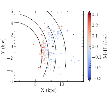
Figure 16: Galactocentric cartesian XY projection of the position of the stars having $M_{\rm ini}\geq 4M_{\odot}$, $\log g$$<2$ and $Z_{\rm max}<0.5\,{\rm kpc}$. The Galactic centre is located at $(X,Y)=0$ (at the left) and Galactic rotation is going clockwise. The colour code represents the metallicity of the stars, whereas the ‘+’ sign is located at the Sun’s position. The position of the Perseus, Local, Sagittarius and Scutum spiral arms, based on Castro-Ginard et al. (2021) results, are also plotted as black continuous lines.

3.3 Age-metallicity relation as a function of orbital actions

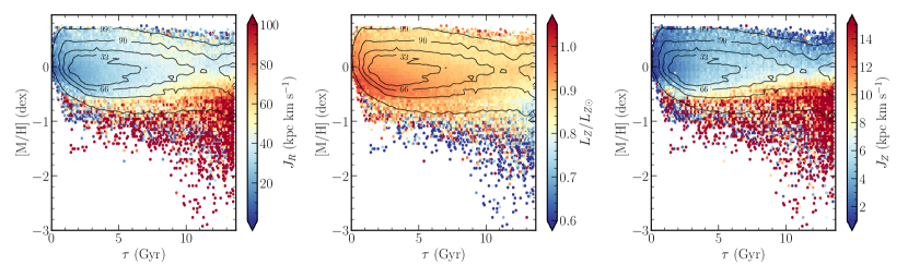
Figure 17: Age-metallicity relations as a function of the radial and vertical actions ($J_{R}$, $J_{Z}$, first and third panel respectively) and normalised angular momentum ($L_{Z}$ normalised by the Sun’s value, middle panel), for stars closer than 1 kpc  from the Sun.

Figure 17 shows the age metallicity-relation we derive for the stars within 1 kpc from the Sun, colour-coded by the three different computed actions. Overall, we find a flat trend over the entire age-range, in agreement with previous studies (e.g. Edvardsson et al., 1993; Casagrande et al., 2011; Bergemann et al., 2014; Feuillet et al., 2019). Young stars ($\tau\lesssim 2\,{\rm Gyr}$) of sub-solar metallicity tend to have low $J_{R}$ and $L_{Z}/L_{Z\odot}$ above one, compatible with stars visiting the Solar neighbourhood on slightly eccentric orbits from the outer disc (we find that these stars have $e<0.1$).

Super-Solar metallicity stars are found at all ages, with perhaps a slight decrease of their number for ages above $10\,{\rm Gyr}$ that may be due to our age prior. However, it is worth noticing that whereas the youngest super-solar metallicity stars have low $J_{R}$ and $L_{Z}/L_{Z\odot}$ close to 0.9, the older ones have on average a larger radial action and more eccentric orbits ($e>0.3$) suggesting that they just visit the Solar neighbourhood, while being close to their apocentre. Interestingly, we also find old ($\tau>8\,{\rm Gyr}$) metal-rich stars with normalised angular momentum around one and low values of radial and vertical actions. These stars are obvious candidates of objects having experienced churning processes, i.e. stars that moved far from their birthplace without changing their eccentricity, via corotation resonances with the spiral arms or the Galactic bar, (Schönrich & Binney, 2009; Minchev et al., 2013; Kordopatis et al., 2015a).

Finally, we find that metal-poor stars ($\rm{[M/H]}<-1\,{\rm dex}$) within 1 kpc  from the Sun are predominantly old, with large radial and vertical actions and low angular momenta, as one would expect for typical halo stars.

3.4 Age-velocity dispersion and $Z_{\rm max}$-metallicity relations

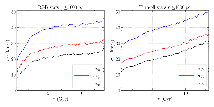
Figure 18: Age-velocity dispersion for the RGB stars (left) and for the turn-off stars (right) closer than $1\,{\rm kpc}$ from the Sun. A clear trend is found in both samples, for each velocity component. However, the fact that these trends do not exhibit the same shape, highlights the different precisions achieved for each stellar type: RGB stars tend to have under-estimated ages for old stars, whereas the younger TO stars tend to have over-estimated ages.

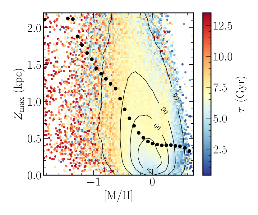
Figure 19: Maximum distance from the Galactic plane reached during a star’s orbit ($Z_{\rm max}$, in  kpc) versus metallicity, colour-coded by age (in Gyr). A clear increase of $Z_{\rm max}$ as a function of metallicity and age can be seen from the black dots on the figure that represent the running mean. This trend is compatible with what one would expect for a transition between thin and thick discs and between thick disc and halo.

Figure 18 shows the age-velocity dispersion relation of our RGB sample (left) and our turn-off sample (right), for stars closer than $1\,{\rm kpc}$ from the Sun. In agreement with previous results (e.g. Aumer & Binney, 2009), we find a clear increase of the velocity dispersions with age, which is even more pronounced when selecting only the turn-off stars. The trend for old stars is starker for the turn-off sample, whereas the giants seem to have a stronger trend at the young side. These different behaviours are in agreement with the ones found in Sect. 2.7, using the APOKASC-2 and Casagrande et al. (2011) datasets, that suggest that old giants tend to have under-estimated ages, whereas very young turn-off stars tend to have over-estimated ages.

Figure 20: Calibrated $\rm[\alpha/Fe]$ versus [M/H], in $3\,{\rm Gyr}$ age-bins for giant stars ($\log g$$<3.5$) closer than $1.5\,{\rm kpc}$ from the Sun. The contour lines inside each panel have been evaluated for the sample considering all the age ranges, represented at the bottom-right panel. The colour-code corresponds to the maximum distance above the Galactic plane that a star can reach during its orbit.

Similarly, Fig. 19 shows the maximum distance from the Galactic plane reached during a star’s orbit as a function of metallicity, colour-coded by age. Black circles represent the running mean in bins of [M/H]. It can be seen that stars with metallicities greater than $-0.2\,{\rm dex}$ tend to be young ($\tau<5\,{\rm Gyr}$) and confined in a thin disc configuration ($Z_{\rm max}<0.3\,{\rm kpc}$) whereas stars with $-0.2<\rm{[M/H]}<-1\,{\rm dex}$ have $Z_{\rm max}<1.1\,{\rm kpc}$ and are globally younger than 10 Gyr, in agreement with the thick disc properties in the solar neighbourhood (e.g. Bensby et al., 2014; Haywood et al., 2018).

3.5 Chemical enrichment of the Galactic disc

A different way to show the wealth of information in our sample is shown in Fig. 20, where we plot the $\rm[\alpha/Fe]-\rm{[M/H]}$ space, in various age-bins, as a function of the orbital parameters (in this case, $Z_{\rm max}$). The $\rm[\alpha/Fe]$ precision of GSP-Spec  is not sufficient to separate the well-known thin and thick disc chemical sequences (see for example Kordopatis et al., 2015b, obtained with high-resolution Gaia-ESO spectra), nevertheless one can see that young stars have in majority low $\rm[\alpha/Fe]$ ratios ($<0.2$), high metallicity ($>-0.5$) and low $Z_{\rm max}$. As look-back time (i.e. age) increases, lower metallicity and higher $\rm[\alpha/Fe]$ regions get populated, with the low metallicity tail exhibiting the largest $Z_{\rm max}$ values. Chemical evolution models can then be fitted to these trends, in order to unfold the star formation history of Galaxy, together with its gas infall history.

In addition to the inner evolution of the Milky Way, our dataset also allows to probe accreted populations present in the surveyed volume. For example, low-metallicity and low-$\rm[\alpha/Fe]$ stars with high $Z_{\rm max}$, associated to Gaia-Enceladus-Sausage (Belokurov et al., 2018; Helmi et al., 2018) stars are detected starting from $\tau>3\,{\rm Gyr}$ (with possible traces even below that we believe are sub-giants with under-estimated ages). Interestingly, the plot also shows some low-metallicity ($\rm{[M/H]}<-0.6\,{\rm dex}$) $\alpha-$enhanced ($\rm[\alpha/Fe]>0.55\,{\rm dex}$) and low-$Z_{\rm max}$ ($<0.3\,{\rm kpc}$) stars present at all age bins. We find that these stars are in majority targets with $T_{\rm eff}$$>6000$ K and similar $\log g$$\sim 3.5$ (also seen at the top left plot of Fig. 8). The true existence of these targets will have to be investigated further.

4 Conclusions

Using the calibrated atmospheric parameters derived from Gaia spectra and the GSP-Spec module, the photometry from 2MASS and Gaia-EDR3, and Bayesian line-of-sight distances estimated using Gaia-EDR3 parallaxes, we derived ages, initial masses and absolute magnitudes for $\sim$ 5 million targets in four different ways, depending on different combinations of parameters to project on isochrones. We propose a way to combine these different estimations, and publish a compiled catalogue of best projected parameters and their uncertainties.

We note that the reliability of the projected parameters is closely related to the one of the input data and their associated uncertainties. Indeed, biases in $T_{\rm eff}$, $\log g$, [M/H] or distance modulus, and/or underestimated errors on them, may lead (depending on the stellar evolutionary phase) to biases on the output ages and masses. For this reason, a careful consideration of GSP-Spec’s flags on the atmospheric parameters is necessary, according to the user’s objectives, in order to chose the parameters with the desired reliability (see Table. 2 of Recio-Blanco et al. 2022).

Tests made comparing our ages and masses with reference catalogues of field stars, open clusters and globular clusters suggest that our code performs well, provided a filtering on the estimated relative age uncertainty (that we suggest $<$ 50 per cent), except for the older giants, for which ages tend to be under-estimated. Ages are found to be the most reliable for turn-off stars, even when the GSP-Spec parameters have large uncertainties, whereas age estimations for giants and main-sequence stars are also retrieved reliably (with uncertainties of the order of 2 Gyr) provided the extinction towards the star’s line-of sight is smaller than $A_{V}\lesssim 2.5$ mag. Initial stellar masses are retrieved robustly for main-sequence and turn-off stars (dispersions compared to literature of the order of $0.1\,M_{\odot}$), whereas a filtering based on the age uncertainty of the giants is necessary to get reliable masses for the latter (dispersions compared to literature of the order of $0.3M_{\odot}$).

We complete our catalogue with Galactocentric positions and velocities as well as orbital parameters (actions, eccentricities, apocenters, pericenters, maximum distance from the Galactic plane) evaluated for the entire RVS sample, using an axisymmetric Galactic potential and commonly used orbital derivation methods and codes. The catalogue, publicly available, is described in Table 3.

Appendix A Output catalogue format

Table 3: Description of the columns of the published catalogue

Name of column	Description	Units
source_id	Gaia DR3 source ID	–
age	Inferred age	Gyr
age_error	Uncertainty on the inferred age	Gyr
m_ini	Inferred initial stellar mass	$M_{\odot}$
m_ini_error	Inferred uncertainty on the initial stellar mass	$M_{\odot}$
teff	Adopted projected $T_{\rm eff}$	K
logg	Adopted projected $\log g$	dex
meta	Adopted projected [M/H]	dex
p_flavour	Adopted projection flavour for inferred ages and masses
G	Inferred absolute G magnitude	mag
G_BP	Inferred absolute $G_{{BP}}$ magnitude	mag
G_RP	Inferred absolute $G_{{RP}}$ magnitude	mag
ebprp	Inferred reddening using the projected $G_{{BP}}$ and $G_{{RP}}$	mag
ebprp_error	Uncertainty on the inferred reddening	mag
*$\_$spec	Parameters adopting the calibrated GSP-Spec parameters only
*$\_$speck	Parameters adopting the calibrated GSP-Spec parameters and the $K_{s}$ absolute magnitude
*$\_$specjhk	Parameters adopting the calibrated GSP-Spec parameters and the $J,H,K_{s}$ absolute magnitudes
*$\_$specjhkg	Parameters adopting the calibrated GSP-Spec parameters and the $J,H,K_{s},G$ absolute magnitudes
x_med_dgeo	Median galactocentric Cartesian X position	kpc
y_med_dgeo	Median galactocentric Cartesian Y position	kpc
z_med__dgeo	Median galactocentric Cartesian Z position	kpc
r_med_dgeo	Median heliocentric line-of-sight distance with geometric prior from Bailer-Jones et al. (2021)	pc
vr_med_dgeo	Median galactocentric radial velocity obtained using r_med_dgeo	${\rm\,{\rm km\leavevmode\nobreak\ s^{-1}}}$
vphi_med_dgeo	Median galactocentric azimuthal velocity obtained using r_med_dgeo	$\,{\rm km\leavevmode\nobreak\ s^{-1}}$
vz_med_dgeo	Median galactocentric vertical velocity obtained using r_med_dgeo	$\,{\rm km\leavevmode\nobreak\ s^{-1}}$
jr_med_dgeo	Median radial action obtained using r_med_dgeo	$\,{\rm kpc}\,{\rm km\leavevmode\nobreak\ s^{-1}}$
jphi_med_dgeo	Median angular momentum (i.e. azimuthal action) obtained using r_med_dgeo	$\,{\rm kpc}\,{\rm km\leavevmode\nobreak\ s^{-1}}$
jz_med_dgeo	Median vertical action obtained using r_med_dgeo	$\,{\rm kpc}\,{\rm km\leavevmode\nobreak\ s^{-1}}$
zmax_med_dgeo	Median maximum distance from the galactic plane obtained using r_med_dgeo	kpc
rapo_med_dgeo	Median apogalactic radius reached by the star, obtained using r_med_dgeo	kpc
rperi_med_dgeo	Median perigalactic radius reached by the star, obtained using r_med_dgeo	kpc
e_med_dgeo	Median eccentricity, obtained using r_med_dgeo	kpc
*_upper_dgeo	Upper confidence limit of the parameters
*_lower_dgeo	Lower confidence limit of the parameters
*_dphotogeo	Parameters obtained using the photogeometric distances from Bailer-Jones et al. (2021)

Appendix B Results of the isochrone projection with extinction

Figures 21 to 23 are similar to Fig. 3. They consider only the speck, specjhk and specjhkg projections, with Q50 uncertainties in $T_{\rm eff}$, $\log g$  and [M/H], and uncertainties in $J,H,K_{s}$ and $G$ as indicated at the top left corner of each plot. The input magnitudes are reddened according to the extinction $A_{V}$ labelled within each plot.

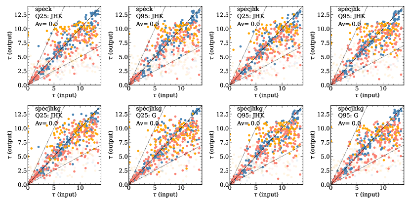
Figure 21: Comparison of the input ages versus the output ones, for the speck, specjhk and specjhkg projections, with Q50 uncertainties in $T_{\rm eff}$, $\log g$  and [M/H], and uncertainties in $J,H,K_{s}$ and $G$ as indicated at the top left corner of each plot. No interstellar extinction is considered here.

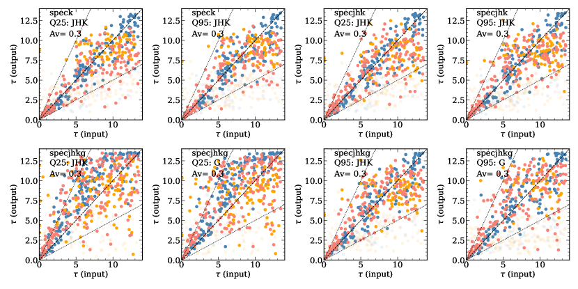
Figure 22: Similar to Fig. 21 with an extinction of $A_{V}=0.3$ mag.

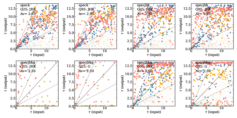
Figure 23: Similar to Fig. 21 with an extinction of $A_{V}=2.5$ mag.

Appendix C Open and globular cluster plots

Figures 24 and 25 show targets selected as being part of open and globular clusters, in the $T_{\rm eff}$-$\log g$  space, as well as in the $T_{\rm eff}$-$M_{\rm K_{s}}$ space. In red are plotted the isochrones with metallicity and age equal to the mean GSP-Spec (calibrated) metallicity and mean derived age of the cluster stars, whereas in black we plot the isochrones for the reference age (12 Gyr in the case of the globular clusters).

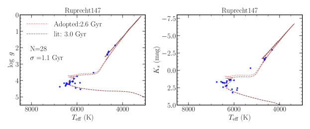
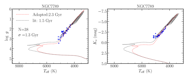
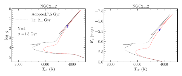
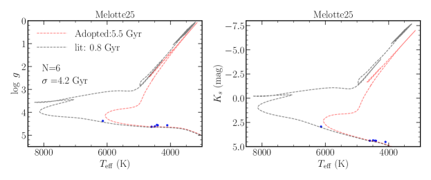
Figure 24: $T_{\rm eff}$-$\log g$ (left) and $T_{\rm eff}$-$M_{\rm K_{s}}$ (right) diagrams for few cherry-picked open clusters.The isochrones of the adopted mean age (in red) and the reference age from Cantat-Gaudin et al. (2020) are plotted in red and black, respectively, for the mean metallicity of the cluster as derived from the calibrated GSP-Spec values. The first two rows show examples for which our ages and the literature ones are in good agreement. The bottom two rows show the opposite: for NGC2112 our solution fits better the data than the younger isochrone, pointing towards offsets in the input $T_{\rm eff}$, [M/H], or distance modulus. For NGC7789, our solution is not reliable, since main-sequence stars do not constrain enough the ages.

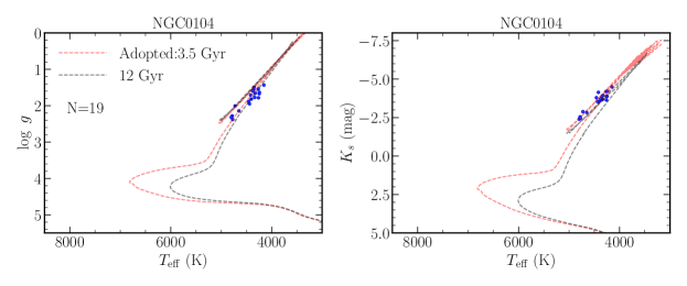
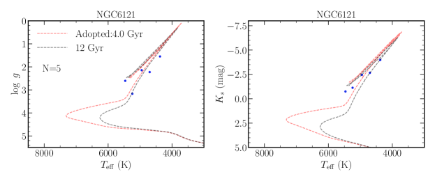
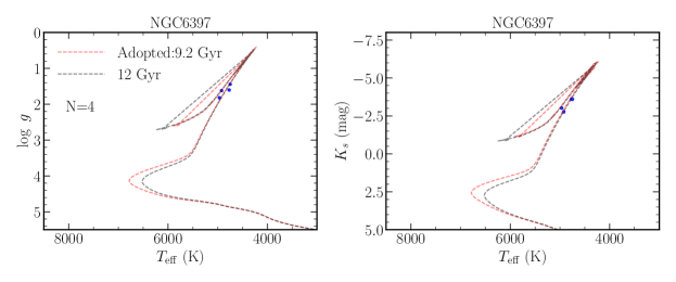
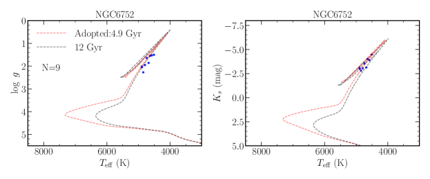
Figure 25: $T_{\rm eff}$-$\log g$ (left) and $T_{\rm eff}$-$M_{\rm K_{s}}$ (right) diagrams for few cherry-picked globular clusters. Candidate stars have been selected based on the results of Gaia Collaboration et al. (2018). The isochrones with the adopted mean age (in red) and for 12 Gyr are plotted in red and black, respectively, for the mean metallicity of the cluster as derived from the calibrated GSP-Spec values.

References

- Anders et al. (2019) Anders, F., Khalatyan, A., Chiappini, C., et al. 2019, A&A, 628, A94
- Andrae et al. (2018) Andrae, R., Fouesneau, M., Creevey, O., et al. 2018, A&A, 616, A8
- Andrae et al. (2022) Andrae, R., Fouesneau, M., Sordo, R., et al. 2022, arXiv e-prints, arXiv:2206.06138
- Astropy Collaboration et al. (2018) Astropy Collaboration, Price-Whelan, A. M., Sipőcz, B. M., et al. 2018, AJ, 156, 123
- Astropy Collaboration et al. (2013) Astropy Collaboration, Robitaille, T. P., Tollerud, E. J., et al. 2013, A&A, 558, A33
- Aumer & Binney (2009) Aumer, M. & Binney, J. J. 2009, MNRAS, 397, 1286
- Bailer-Jones (2015) Bailer-Jones, C. A. L. 2015, PASP, 127, 994
- Bailer-Jones et al. (2013) Bailer-Jones, C. A. L., Andrae, R., Arcay, B., et al. 2013, A&A, 559, A74
- Bailer-Jones et al. (2021) Bailer-Jones, C. A. L., Rybizki, J., Fouesneau, M., Demleitner, M., & Andrae, R. 2021, AJ, 161, 147
- Basu & Antia (1997) Basu, S. & Antia, H. M. 1997, MNRAS, 287, 189
- Belokurov et al. (2018) Belokurov, V., Erkal, D., Evans, N. W., Koposov, S. E., & Deason, A. J. 2018, MNRAS, 478, 611
- Bennett & Bovy (2019) Bennett, M. & Bovy, J. 2019, MNRAS, 482, 1417
- Bensby et al. (2014) Bensby, T., Feltzing, S., & Oey, M. S. 2014, A&A, 562, A71
- Bergemann et al. (2014) Bergemann, M., Ruchti, G. R., Serenelli, A., et al. 2014, A&A, 565, A89
- Binney (2012) Binney, J. 2012, MNRAS, 426, 1324
- Binney et al. (2014) Binney, J., Burnett, B., Kordopatis, G., et al. 2014, MNRAS, 437, 351
- Bonifacio et al. (2000) Bonifacio, P., Monai, S., & Beers, T. C. 2000, AJ, 120, 2065
- Bovy (2015) Bovy, J. 2015, ApJS, 216, 29
- Bovy et al. (2019) Bovy, J., Leung, H. W., Hunt, J. A. S., et al. 2019, MNRAS, 490, 4740
- Bressan et al. (2012) Bressan, A., Marigo, P., Girardi, L., et al. 2012, MNRAS[arXiv:1208.4498]
- Caffau et al. (2011) Caffau, E., Ludwig, H. G., Steffen, M., Freytag, B., & Bonifacio, P. 2011, Sol. Phys., 268, 255
- Cantat-Gaudin et al. (2020) Cantat-Gaudin, T., Anders, F., Castro-Ginard, A., et al. 2020, A&A, 640, A1
- Cardelli et al. (1989) Cardelli, J. A., Clayton, G. C., & Mathis, J. S. 1989, ApJ, 345, 245
- Carraro et al. (2002) Carraro, G., Barbon, R., & Boschetti, C. S. 2002, MNRAS, 336, 259
- Casagrande et al. (2011) Casagrande, L., Schönrich, R., Asplund, M., et al. 2011, A&A, 530, A138
- Castro-Ginard et al. (2021) Castro-Ginard, A., McMillan, P. J., Luri, X., et al. 2021, A&A, 652, A162
- Chen et al. (2015) Chen, Y., Bressan, A., Girardi, L., et al. 2015, MNRAS, 452, 1068
- Creevey et al. (2022) Creevey, O. L., Sordo, R., Pailler, F., et al. 2022, arXiv e-prints, arXiv:2206.05864
- Delchambre et al. (2022) Delchambre, L., Bailer-Jones, C. A. L., Bellas-Velidis, I., et al. 2022, arXiv e-prints, arXiv:2206.06710
- Edvardsson et al. (1993) Edvardsson, B., Andersen, J., Gustafsson, B., et al. 1993, A&A, 275, 101
- Feuillet et al. (2020) Feuillet, D. K., Feltzing, S., Sahlholdt, C. L., & Casagrande, L. 2020, MNRAS, 497, 109
- Feuillet et al. (2019) Feuillet, D. K., Frankel, N., Lind, K., et al. 2019, MNRAS, 489, 1742
- Fitzgerald (1968) Fitzgerald, M. P. 1968, AJ, 73, 983
- Fouesneau et al. (2022) Fouesneau, M., Andrae, R., Sordo, R., & Dharmawardena, T. 2022, dustapprox
- Fouesneau et al. (2022) Fouesneau, M., Frémat, Y., Andrae, R., et al. 2022, arXiv e-prints, arXiv:2206.05992
- Freeman & Bland-Hawthorn (2002) Freeman, K. & Bland-Hawthorn, J. 2002, ARA&A, 40, 487
- Gaia Collaboration et al. (2018) Gaia Collaboration, Helmi, A., van Leeuwen, F., et al. 2018, A&A, 616, A12
- Gaia Collaboration, Antoja, T. et al. (2021) Gaia Collaboration, Antoja, T., McMillan, P. J., Kordopatis, G., et al. 2021, A&A, 649, A8
- Gaia Collaboration, Brown, A. et al. (2018) Gaia Collaboration, Brown, A., Vallenari, A., Prusti, T., et al. 2018, A&A, 616, A1
- Gaia Collaboration, Brown, A. et al. (2021) Gaia Collaboration, Brown, A., Vallenari, A., Prusti, T., et al. 2021, A&A, 649, A1
- Gaia Collaboration, Brown A., et al. (2016) Gaia Collaboration, Brown A.,, Vallenari, A., Prusti, T., et al. 2016, A&A, 595, A2
- Gaia Collaboration, Prusti, T. et al. (2016) Gaia Collaboration, Prusti, T., de Bruijne, J. H. J., Brown, A. G. A., et al. 2016, A&A, 595, A1
- Gaia Collaboration, Recio-Blanco et al. (2022) Gaia Collaboration, Recio-Blanco, Kordopatis, G., de Laverny, P., et al. 2022, arXiv e-prints, arXiv:2206.05534
- Gaia Collaboration, Schultheis et al. (2022) Gaia Collaboration, Schultheis, Zhao, H., Zwitter, T., et al. 2022, arXiv e-prints, arXiv:2206.05536
- Gaia Collaboration, Vallenari, A. & Brown (2022) Gaia Collaboration, Vallenari, A. & Brown, A. G. A. 2022, A&A in prep.
- Gravity Collaboration et al. (2020) Gravity Collaboration, Abuter, R., Amorim, A., et al. 2020, A&A, 636, L5
- Green (2018) Green, G. 2018, The Journal of Open Source Software, 3, 695
- Green et al. (2019) Green, G. M., Schlafly, E., Zucker, C., Speagle, J. S., & Finkbeiner, D. 2019, ApJ, 887, 93
- Hayden et al. (2017) Hayden, M. R., Recio-Blanco, A., de Laverny, P., Mikolaitis, S., & Worley, C. C. 2017, A&A, 608, L1
- Haywood et al. (2018) Haywood, M., Di Matteo, P., Lehnert, M. D., et al. 2018, ApJ, 863, 113
- Helmi et al. (2018) Helmi, A., Babusiaux, C., Koppelman, H. H., et al. 2018, Nature, 563, 85
- Hidalgo et al. (2018) Hidalgo, S. L., Pietrinferni, A., Cassisi, S., et al. 2018, ApJ, 856, 125
- Jørgensen & Lindegren (2005) Jørgensen, B. R. & Lindegren, L. 2005, A&A, 436, 127
- Kalberla & Kerp (2009) Kalberla, P. M. W. & Kerp, J. 2009, ARA&A, 47, 27
- Kharchenko et al. (2013) Kharchenko, N. V., Piskunov, A. E., Schilbach, E., Röser, S., & Scholz, R. D. 2013, A&A, 558, A53
- Kordopatis et al. (2016) Kordopatis, G., Amorisco, N. C., Evans, N. W., Gilmore, G., & Koposov, S. E. 2016, MNRAS, 457, 1299
- Kordopatis et al. (2015a) Kordopatis, G., Binney, J., Gilmore, G., et al. 2015a, MNRAS, 447, 3526
- Kordopatis et al. (2013) Kordopatis, G., Hill, V., Irwin, M., et al. 2013, A&A, 555, A12
- Kordopatis et al. (2011) Kordopatis, G., Recio-Blanco, A., de Laverny, P., et al. 2011, A&A, 535, A107
- Kordopatis et al. (2020) Kordopatis, G., Recio-Blanco, A., Schultheis, M., & Hill, V. 2020, A&A, 643, A69
- Kordopatis et al. (2015b) Kordopatis, G., Wyse, R. F. G., Gilmore, G., et al. 2015b, A&A, 582, A122
- Lallement et al. (2014) Lallement, R., Vergely, J. L., Valette, B., et al. 2014, A&A, 561, A91
- Laporte et al. (2020) Laporte, C. F. P., Belokurov, V., Koposov, S. E., Smith, M. C., & Hill, V. 2020, MNRAS, 492, L61
- Leung & Bovy (2019) Leung, H. W. & Bovy, J. 2019, MNRAS, 483, 3255
- Lindegren (2018) Lindegren, L. 2018, gAIA-C3-TN-LU-LL-124
- Luri et al. (2018) Luri, X., Brown, A. G. A., Sarro, L. M., et al. 2018, A&A, 616, A9
- Mackereth & Bovy (2018) Mackereth, J. T. & Bovy, J. 2018, PASP, 130, 114501
- Magrini et al. (2017) Magrini, L., Randich, S., Kordopatis, G., et al. 2017, A&A, 603, A2
- Magrini et al. (2018) Magrini, L., Spina, L., Randich, S., et al. 2018, A&A, 617, A106
- Marigo et al. (2013) Marigo, P., Bressan, A., Nanni, A., Girardi, L., & Pumo, M. L. 2013, MNRAS, 434, 488
- McMillan (2017) McMillan, P. J. 2017, MNRAS, 465, 76
- McMillan et al. (2018) McMillan, P. J., Kordopatis, G., Kunder, A., et al. 2018, MNRAS, 477, 5279
- Miglio et al. (2013) Miglio, A., Chiappini, C., Morel, T., et al. 2013, MNRAS, 429, 423
- Minchev et al. (2013) Minchev, I., Chiappini, C., & Martig, M. 2013, A&A, 558, A9
- Myeong et al. (2019) Myeong, G. C., Vasiliev, E., Iorio, G., Evans, N. W., & Belokurov, V. 2019, MNRAS, 488, 1235
- Naidu et al. (2020) Naidu, R. P., Conroy, C., Bonaca, A., et al. 2020, ApJ, 901, 48
- O’Donnell (1994) O’Donnell, J. E. 1994, ApJ, 422, 158
- Pastorelli et al. (2020) Pastorelli, G., Marigo, P., Girardi, L., et al. 2020, MNRAS, 498, 3283
- Pinsonneault et al. (2018) Pinsonneault, M. H., Elsworth, Y. P., Tayar, J., et al. 2018, ApJS, 239, 32
- Queiroz et al. (2018) Queiroz, A. B. A., Anders, F., Santiago, B. X., et al. 2018, MNRAS, 476, 2556
- Recio-Blanco et al. (2014) Recio-Blanco, A., de Laverny, P., Kordopatis, G., et al. 2014, A&A, 567, A5
- Recio-Blanco et al. (2022) Recio-Blanco, A., de Laverny, P., Palicio, P. A., et al. 2022, arXiv e-prints, arXiv:2206.05541
- Reid & Brunthaler (2020) Reid, M. J. & Brunthaler, A. 2020, ApJ, 892, 39
- Riello et al. (2021) Riello, M., de Angeli, F., Evans, D. W., et al. 2021, VizieR Online Data Catalog, J/A+A/649/A3
- Rosenfield et al. (2016) Rosenfield, P., Marigo, P., Girardi, L., et al. 2016, ApJ, 822, 73
- Salaris et al. (1993) Salaris, M., Chieffi, A., & Straniero, O. 1993, ApJ, 414, 580
- Sanders & Binney (2016) Sanders, J. L. & Binney, J. 2016, MNRAS, 457, 2107
- Sanders & Das (2018) Sanders, J. L. & Das, P. 2018, MNRAS, 481, 4093
- Santos-Peral et al. (2021) Santos-Peral, P., Recio-Blanco, A., Kordopatis, G., Fernández-Alvar, E., & de Laverny, P. 2021, A&A, 653, A85
- Schlegel et al. (1998) Schlegel, D. J., Finkbeiner, D. P., & Davis, M. 1998, ApJ, 500, 525
- Schönrich & Binney (2009) Schönrich, R. & Binney, J. 2009, MNRAS, 396, 203
- Schönrich et al. (2019) Schönrich, R., McMillan, P., & Eyer, L. 2019, MNRAS, 487, 3568
- Schultheis et al. (2015) Schultheis, M., Kordopatis, G., Recio-Blanco, A., et al. 2015, A&A, 577, A77
- Schultheis et al. (2017) Schultheis, M., Rojas-Arriagada, A., García Pérez, A. E., et al. 2017, A&A, 600, A14
- Skrutskie et al. (2006) Skrutskie, M. F., Cutri, R. M., Stiening, R., et al. 2006, AJ, 131, 1163
- Soderblom (2010) Soderblom, D. R. 2010, ARA&A, 48, 581
- Stello et al. (2022) Stello, D., Saunders, N., Grunblatt, S., et al. 2022, MNRAS, 512, 1677
- Tang et al. (2014) Tang, J., Bressan, A., Rosenfield, P., et al. 2014, MNRAS, 445, 4287
- Valentini et al. (2019) Valentini, M., Chiappini, C., Bossini, D., et al. 2019, A&A, 627, A173
- VandenBerg et al. (2013) VandenBerg, D. A., Brogaard, K., Leaman, R., & Casagrande, L. 2013, ApJ, 775, 134
- Zhao et al. (2021) Zhao, H., Schultheis, M., Recio-Blanco, A., et al. 2021, A&A, 645, A14
- Zwitter et al. (2010) Zwitter, T., Matijevič, G., Breddels, M. A., et al. 2010, A&A, 522, A54