Arnoldi-based orthonormal and hierarchical divergence-free polynomial basis and its applications

Abstract

This paper presents a methodology to construct a divergence-free polynomial basis of an arbitrary degree in a simplex (triangles in 2D and tetrahedra in 3D) of arbitrary dimension. It allows for fast computation of all numerical solutions from degree zero to a specified degree $k$ for certain PDEs. The generated divergence-free basis is orthonormal, hierarchical, and robust in finite-precision arithmetic. At the core is an Arnoldi-based procedure. It constructs an orthonormal and hierarchical basis for multi-dimensional polynomials of degree less than or equal to $k$. The divergence-free basis is generated by combining these polynomial basis functions. An efficient implementation of the hybridized BDM mixed method is developed using these basis functions. Hierarchy allows for incremental construction of the global matrix and the global vector for all degrees (zero to $k$) using the local problem solution computed just for degree $k$. Orthonormality and divergence-free properties simplify the local problem. PDEs considered are Helmholtz, Laplace, and Poisson problems in smooth domains and in a corner domain. These advantages extend to other PDEs such as incompressible Stokes, incompressible Navier-Stokes, and Maxwell equations.

1 Introduction

Divergence-free vector fields occur in several problems. For e.g., the fluid velocity field in an incompressible fluid flow, the solid velocity in an incompressible solid deformation, the magnetic field around an electric current, and the steady state heat flux in a conducting medium with no volumetric sources. Approximating such vector fields using divergence-free basis functions is advantageous. It reduces the number of global degrees of freedom while computing approximate solutions to their partial differential equations (PDEs) (Cockburn et al., 2004, 2010). While interpolating experimental measurements (Gesemann et al., 2016; Agarwal et al., 2021), it yields reconstructed fields that are consistent with the problem physics. This paper discusses a procedure to construct a divergence-free polynomial basis that is well-conditioned, orthonormal, and hierarchical for arbitrary polynomial degree in a simplex.

Below is a simple exercise to construct a linear monomial divergence-free basis for two dimensions. Consider the two dimensional linear monomial basis:

$$\Bigg{\{}\underbrace{\begin{pmatrix}1\\ 0\end{pmatrix}}_{(1)},\underbrace{\begin{pmatrix}0\\ 1\end{pmatrix}}_{(2)},\underbrace{\begin{pmatrix}x\\ 0\end{pmatrix}}_{(3)},\underbrace{\begin{pmatrix}y\\ 0\end{pmatrix}}_{(4)},\underbrace{\begin{pmatrix}0\\ x\end{pmatrix}}_{(5)},\underbrace{\begin{pmatrix}0\\ y\end{pmatrix}}_{(6)}\Bigg{\}}.$$

The basis functions (1), (2), (4), and (5) are divergence-free but (3) and (6) are not. However, basis functions (3) and (6) can be combined as

$$\begin{pmatrix}x\\ 0\end{pmatrix}-\begin{pmatrix}0\\ y\end{pmatrix}=\begin{pmatrix}x\\ -y\end{pmatrix}$$

to be divergence-free. This yields the following linear monomial divergence-free basis:

$$\Bigg{\{}\underbrace{\begin{pmatrix}1\\ 0\end{pmatrix}}_{(1)},\underbrace{\begin{pmatrix}0\\ 1\end{pmatrix}}_{(2)},\underbrace{\begin{pmatrix}y\\ 0\end{pmatrix}}_{(3)},\underbrace{\begin{pmatrix}0\\ x\end{pmatrix}}_{(4)},\underbrace{\begin{pmatrix}x\\ -y\end{pmatrix}}_{(5)}\Bigg{\}}.$$

Similarly, the following quadratic monomial divergence-free basis:

$$\Bigg{\{}\underbrace{\begin{pmatrix}1\\ 0\end{pmatrix}}_{(1)},\underbrace{\begin{pmatrix}0\\ 1\end{pmatrix}}_{(2)},\underbrace{\begin{pmatrix}y\\ 0\end{pmatrix}}_{(3)},\underbrace{\begin{pmatrix}0\\ x\end{pmatrix}}_{(4)},\underbrace{\begin{pmatrix}x\\ -y\end{pmatrix}}_{(5)},\underbrace{\begin{pmatrix}y^{2}\\ 0\end{pmatrix}}_{(6)},\underbrace{\begin{pmatrix}0\\ x^{2}\end{pmatrix}}_{(7)},\underbrace{\begin{pmatrix}x^{2}/2\\ -xy\end{pmatrix}}_{(8)},\underbrace{\begin{pmatrix}-xy\\ y^{2}/2\end{pmatrix}}_{(9)}\Bigg{\}}$$

can be constructed from the two-dimensional quadratic monomial basis. This procedure can be generalized to arbitrary polynomial degree and spatial dimension; see the MATLAB program mondivfreebf in figure 13 of appendix G. However, it turns out that the resulting monomial divergence-free basis functions perform poorly in finite precision arithmetic for high polynomial degrees.

(a)

(b)

(c)

Figure 1: Projection of $(\sin(4\pi x)\cos(4\pi y),-\cos(4\pi x)\sin(4\pi y))$ onto the space of divergence-free polynomials in the unit triangle. (a) Error v/s polynomial degree for the monomial divergence-free basis. (a) Error v/s polynomial degree for the Arnoldi-based divergence-free basis. (c) Contours of $x$-component of the projection computed with the Arnoldi-based divergence-free basis for polynomial degree 40.

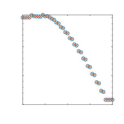
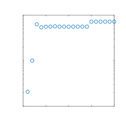
Consider the $L^{2}$ projection of the divergence-free function $\vec{g}=(\sin(4\pi x)\cos(4\pi y),-\cos(4\pi x)\sin(4\pi y))$ onto the space of divergence-free polynomials in the unit triangle defined by the nodes (0,0), (1,0), and (0,1). Figure 1a shows the maximum error in the projection computed with the monomial divergence-free basis as a function of polynomial degree. The error decreases to around $10^{-3}$ for degree 20. After degree 20, only 1-3 significant digits of accuracy are obtained. This is because of finite precision error. The condition number of the mass matrix with the monomial divergence-free basis increases exponentially with degree, and therefore, the finite precision error also grows exponentially.

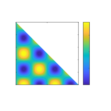
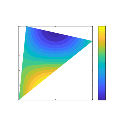
Suppose, instead of using the monomial divergence-free basis, we use the proposed divergence-free basis. The projection error decreases all the way down to machine precision; see figure 1b. The contours of $x$-component of the projection computed with this basis are shown in figure 1c for degree 40. This demonstrates the robustness of our divergence-free basis in finite precision arithmetic. To build a well-conditioned divergence-free basis, we combine orthonormal polynomial (Gautschi, 2004) basis functions. To generate these input orthonormal polynomial basis functions in a simplex of arbitrary dimension, we propose a simple Arnoldi-based procedure. This procedure is an extension of the one-dimensional Arnoldi/Stieltjes process (Gautschi, 1982) discussed in lecture 37 of Trefethen and Bau III (1997).

(a)

(b)

(c)

Figure 2: Laplace problem with corner singularity. (a) Mesh. (b) Error in the computed scalar at $(0.99,0.99)$ v/s polynomial degree. (c) Contours of $x$-component of the flux computed with polynomial degree eight.

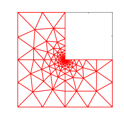
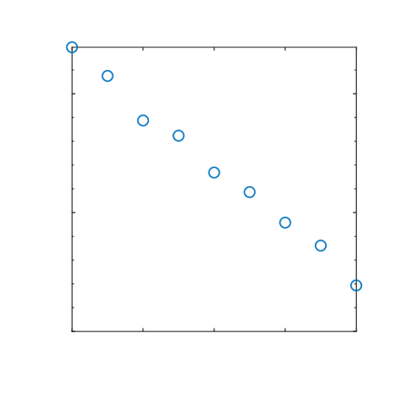
The advantages of using our basis for numerical solutions of PDEs are demonstrated for the Laplace problem with corner singularity. This problem is taken from Gopal and Trefethen (2019). The domain is L-shaped (see figure 2a). Dirichlet boundary conditions of $x^{2}$ are used on all the boundaries, and the resulting solution has a singularity at the re-entrant corner $(1,1)$. In $2019$, Gopal and Trefethen (2019) called for finite element method (FEM) solutions to this problem. Specifically, they asked for a computation of the scalar at $(0.99,0.99)$ – a point close to the re-entrant corner. They report ‘…all respondents were able to calculate a solution to two to four significant digits of accuracy, only two came close to eight digits. For example, one researcher used 158,997 fifth-order triangular elements near the re-entrant corner and achieved six correct digits …’. Our results computed by using the proposed divergence-free basis in the hybridized Brezzi-Douglas-Marini (BDM) (Brezzi et al., 1985) mixed finite element method (FEM) are shown in figure 2. The approximation with polynomial degree eight is accurate up to 12 significant digits at the point $(0.99,0.99)$ and we use just 1000 elements (mesh shown in figure 2a). It takes just around four seconds to compute all approximations from polynomial degree zero to eight (all computations for this paper are performed in MATLAB on a desktop workstation with Intel(R) Core(TM) i7-8700 CPU @ 3.20GHz and six cores).

We can compute all approximations in such a short time because our basis is hierarchical and orthonormal. Hierarchy allows us to solve the local problem in the hybridized BDM method just for polynomial degree eight and use its solution to incrementally construct the element (and global) matrices and vectors for all polynomial degrees from zero to eight. Orthonormality simplifies the local problem solutions to just inner products instead of requiring matrix inversions. Therefore, our computation is fast. Furthermore, the results demonstrate exponential convergence near the singularity. Gopal and Trefethen (2019) note that hp-adaptive FEM can achieve exponential convergence near singularities but requires advanced implementations. We, on the other hand, do not require such advanced implementation. These advantages of our basis extend to several other PDEs and to other hybridized FEM methods.

A word on the one-dimensional Arnoldi/Stieltjes process discussed in Trefethen and Bau III (1997). The development of this process begins by recognizing that the space of one-dimensional polynomials of degree less than or equal to $k$ given by span$\{1,x,x^{2},...,x^{k}\}$ is a Krylov subspace. Define the coordinate operator $\widehat{x}$ as the operator that maps a one-dimensional polynomial $f$ to another polynomial $xf$. The one-dimensional polynomial space can then be rewritten as the Krylov subspace span$\{1,\widehat{x}1,\widehat{x}^{2}1,...,\widehat{x}^{k}1\}$ generated by the linear operator $\widehat{x}$ and the starting polynomial ‘1’. The one-dimensional Arnoldi/Steiljets process to generate an orthonormal basis for this space is:

1:$q_{1}=1$

2:for $j=1,\dots,k$ do

3:     $v=\widehat{x}q_{j}$

4:     for $i=1,\dots,j$ do

5:         $h_{i,j}=\int_{0}^{1}q_{i}^{*}v\,dx$

6:         $v=v-h_{i,j}q_{i}$

7:     end for

8:     $h_{j+1,j}=\left(\int_{0}^{1}|v|^{2}\,dx\right)^{1/2}$

9:     $q_{j+1}=v/h_{j+1,j}$

10:end for

The generated polynomials $q_{1},\dots,q_{k+1}$ are a basis orthonormal in the $L^{2}$ inner-product for polynomials of degree less than or equal to $k$ in the interval $[0,1]$. Since the operator $\widehat{x}$ is hermitian, the above Arnoldi process can be simplified to a Lanczos process. However, such simplifications are not performed usually for numerical stability reasons. We note that this process is rarely used to generate the one-dimensional polynomials orthonormal in the $L^{2}$ inner-product, i.e., the Legendre polynomials. Instead, analytical expressions for the coefficients $h_{i,j}$, also called the recurrence relations, are used. Nevertheless, it still is a powerful technique to generate one-dimensional polynomials orthonormal for an arbitrary weighted inner-product.

The situation is a little different in a simplex of dimension larger than one. Recurrence relations do exist for the coefficients analogous to $h_{i,j}$ to construct orthonormal polynomials in triangles and tetrahedra (Olver et al., 2020; Sherwin and Karniadakis, 1995; Dubiner, 1991). However, these are complicated compared to the one dimensional relations. Our Arnoldi-based process is a simple alternative implementable in just a few lines of MATLAB code. An advantage of this process is that it can construct an orthonormal basis not just for the $L^{2}$ inner-product but for arbitrary weighted inner-product and for even discrete inner-products. Another advantage is that it extends to a simplex of arbitrary dimension.

The proposed Arnoldi-based process can also be seen as an extension of the ‘Vandermonde with Arnoldi’ idea of Brubeck et al. (2021). Brubeck et al. (2021) considered the one-dimensional Vandermonde matrix problem and showed that despite using the well-conditioned Chebyshev points to construct the Vandermonde matrix, the computed approximation at high polynomial degrees can be significantly contaminated by round-off error. To remedy this issue, they proposed an Arnoldi-based procedure to solve the Vandermonde matrix problem. Using this procedure, they were able to compute approximations that were accurate up to machine precision. The $L^{2}$ projection numerical experiment whose results are displayed in figure 1 demonstrate a similar accuracy in finite precision arithmetic for the proposed Arnoldi-based process.

Finally, we note that Ainsworth and Fu (2018) constructed a divergence-free basis for triangles and tetrahedra using Bernstein polynomials. However, their construction yields a non-orthogonal basis, thus requiring matrix inversions in local problem solution in hybridized FEM methods while ours requires only inner products. Furthermore, their divergence-free basis is not hierarchical. Therefore, the local problem solution, construction of element matrices and vectors need to be computed separately for each polynomial degree, while we exploit the basis hierarchy to compute them efficiently.

The rest of the paper is organized as follows. In section 2, we present the proposed method. Its numerical implementation is given in section 3. Some remarks on the proposed method are made in section 4. Section 5 demonstrates some applications of the proposed basis. The paper is summarized in section 6.

2 Divergence-free polynomial basis construction

We are given $N_{ele}$ simplices (also referred to as ‘elements’) in $d$ dimensions. The node coordinate matrix (a matrix whose rows store the coordinate vector of the nodes of the element) of each element $e$ is $X^{(e)}$. We need to construct an orthonormal and hierarchical basis for divergence-free polynomials of degree less than or equal to some prescribed degree $k$ in each of these elements. The required basis is the set of vector-valued polynomials $\bm{\varphi}_{1}^{(e)},\dots,\bm{\varphi}_{n}^{(e)}$ in each element $e$. By an orthonormal basis, we mean that any two divergence-free basis functions $\bm{\varphi}_{i}^{(e)}$ and $\bm{\varphi}_{j}^{(e)}$ of element $e$ satisfy the orthonormality relation $\int_{\Omega^{(e)}}\bm{\varphi}^{(e)}_{i}\cdot\bm{\varphi}^{(e)}_{j}\,d\Omega=\delta_{ij}|\Omega^{(e)}|$, where $\Omega^{(e)}$ denotes the $e^{th}$ element and $|\Omega^{(e)}|$ is its volume. By a hierarchical basis, we mean that the basis functions are generated incrementally for each degree up to $k$. A formal definition of this is that the first $dC_{d}^{j+d}-C_{d}^{j-1+d}$ basis functions form a basis for divergence-free polynomials of degree less than or equal to $j$, where $j$ is any degree satisfying $0\leq j\leq k$. $n$ is the dimension of the basis in each element. It equals $dC_{d}^{k+d}-C_{d}^{k-1+d}$ because the dimension of the set of vector-valued polynomials is $dC_{d}^{k+d}$ and the divergence-free requirement imposes $C_{d}^{k-1+d}$ constraints.

The proposed method can be summarized as follows:

1. Construct the divergence-free basis first in the reference element $\widehat{\Omega}$. This basis is the set of vector-valued polynomials $\bm{\varphi}_{1},\dots,\bm{\varphi}_{n}$, where $\bm{\varphi}_{i}$ is the $i^{th}$ basis function. The reference element is a unit simplex in $d$ dimensions. Its node-coordinate matrix is [zeros$(1,d)$; eye$(d)$] (in MATLAB notation). The goal is to combine polynomial basis functions that are orthonormal in the reference element to generate the divergence-free polynomial basis functions that are also orthonormal in the reference element. The orthonormal polynomial basis is the set of polynomials $q_{1},\dots,q_{p}$, where $p=C_{d}^{k+d}$ and $q_{i}$ is the $i^{th}$ basis function. To ensure that the constructed divergence-free basis functions are hierarchical, this idea is recursively applied for each polynomial degree up to $k$. The required polynomial basis functions ($q_{i}$) are constructed for each degree using an Arnoldi-based procedure. For degree $j=0$, there is only one polynomial basis function and it is $q_{1}=1$. There are three degree zero divergence-free polynomial basis functions given by $\bm{\varphi}_{i}=q_{1}\mathbf{e}_{i}$, where $i=1,\dots,d$. For each degree $j=1,\dots,k$, do Step 1.1 and 1.2.

   1. Compute the polynomial basis functions $q_{p_{j-1}+1},\dots,q_{p_{j}}$ of degree $j$ using the previously computed basis functions $q_{1},\dots,q_{p_{j-1}}$ and the Arnoldi-based procedure given below:

      1:Set $c=p_{j-1}$

      2:for $i=1,\dots,d$ do

      3:     $j^{\prime\prime}=C_{d-i}^{j-1+d-i}$

      4:     for $j^{\prime}=1,\dots,j^{\prime\prime}$ do

      5:         $v=\widehat{x}_{i}q_{p_{j-1}-j^{\prime\prime}+j^{\prime}}$ $\triangleright$ Equivalent of $Aq_{j}$ in the standard Arnoldi

      6:         for $j^{\prime\prime\prime}=1,\dots,c$ do $\triangleright$ Orthogonalization

      7:              $H_{j^{\prime\prime\prime},c}=(\int_{\widehat{\Omega}}q_{j^{\prime\prime\prime}}^{*}v\,d\widehat{\Omega})d!$

      8:              $v=v-H_{j^{\prime\prime\prime},c}q_{j^{\prime\prime\prime}}$

      9:         end for

      10:         $H_{c+1,c}=(\int_{\widehat{\Omega}}|v|^{2}\,\,d\widehat{\Omega})^{1/2}{d!}^{1/2}$

      11:         $q_{c+1}=v/H_{c+1,c}$$\triangleright$ Normalization

      12:         $c=c+1$

      13:     end for

      14:end for

      Here, $p_{j}=C_{d}^{j+d}$. $\widehat{x}_{i}$ is the coordinate operator along the $i^{th}$ direction. It maps a polynomial $f$ to another polynomial $x_{i}f$. The new set of polynomials $q_{1},\dots,q_{p_{j}}$ form a basis for polynomials of degree less than or equal to $j$ (see appendix A for more discussion). The Gram-Schmidt procedure enforces them to be orthonormal to each other. They satisfy the orthonormality relation $\int_{\widehat{\Omega}}q_{i}q_{j}d\widehat{\Omega}=\delta_{ij}1/d!$, where $1/d!$ is the volume of the reference element. The computed $H_{i,j}$s are stored in a matrix $H$ of size $p\times(p-1)$. Similar to the standard Arnoldi (Saad, 2011), $H$ is an upper Hessenberg matrix, i.e., $H_{i,j}=0$ for $i>j+1$.

   2. Compute the divergence-free basis functions $\bm{\varphi}_{n_{j-1}+1},\dots,\bm{\varphi}_{n_{j}}$ of degree $j$ (where $n_{j}=dC_{d}^{j+d}-C_{d}^{j-1+d}$) by combining the polynomial basis functions $q_{1},\dots,q_{p_{j}}$ and using the previously computed divergence-free basis functions $\bm{\varphi}_{1},\dots,\bm{\varphi}_{n_{j-1}}$ as follows:

      1:Expand each $\bm{\varphi}_{\ell}$ as $\bm{\varphi}_{\ell}=\sum_{i=1}^{d}\sum_{r=1}^{p_{j}}N_{(i-1)p+r,\ell}q_{r}\bm{e}_{i},$ for $\ell=n_{j-1}+1,\dots,n_{j}$. Here, $N_{(i-1)p+r,\ell}$ are the coefficients stored in a matrix $N$ of size $dp\times n$.

      2:Compute the coefficients $N_{(i-1)p+r,\ell}$ such that the set of functions $\bm{\varphi}_{n_{j-1}+1},\dots,\bm{\varphi}_{n_{j}}$ are:

      1. divergence-free, i.e., $\int_{\widehat{\Omega}}q_{i}\bm{\nabla}\cdot\bm{\varphi}_{\ell}d\widehat{\Omega}=0$, for $\ell=n_{j-1}+1,\dots,n_{j}$ and $i=1,\dots,p_{j-1}$,

      2. orthonormal, i.e., $\int_{\widehat{\Omega}}\bm{\varphi}_{\ell}\cdot\bm{\varphi}_{\ell^{\prime}}\,d\widehat{\Omega}=\delta_{\ell,\ell^{\prime}}1/d!$, where $\ell=n_{j-1}+1,\dots,n_{j}$, $\ell^{\prime}=1,\dots,n_{j}$, and

      3. linearly independent.

      The new set of vector-valued polynomials $\bm{\varphi}_{1},\dots,\bm{\varphi}_{n_{j}}$ form a orthonormal basis for the divergence-free polynomials of degree less than or equal to $j$. They satisfy the orthonormality relation $\int_{\widehat{\Omega}}\bm{\varphi}_{i}\cdot\bm{\varphi}_{j}d\widehat{\Omega}=\delta_{ij}1/d!$. See appendix B for a discussion on this.

2. Construct the divergence-free basis in each element $e$ using the divergence-free basis in the reference element and the node coordinate matrix $X^{(e)}$ of the element. The basis in element $e$ is given by the set of vector-valued polynomials $\bm{\varphi}^{(e)}_{1},\dots,\bm{\varphi}^{(e)}_{n}$. To ensure that the constructed divergence-free basis is hierarchical, the basis functions are constructed incrementally for each degree up to $k$. For each element $e=1,\dots,N_{ele}$ and for each degree $j=0,\dots,k$, do Step 2.1.

   1. Construct the divergence-free basis functions $\bm{\varphi}^{(e)}_{n_{j-1}+1},\dots,\bm{\varphi}^{(e)}_{n_{j}}$ of degree $j$ using the previously computed basis functions $\bm{\varphi}^{(e)}_{1},\dots,\bm{\varphi}^{(e)}_{n_{j-1}}$ and the reference element basis functions $\bm{\varphi}_{n_{j-1}+1},\dots,\bm{\varphi}_{n_{j}}$ as follows:

      1:Expand each $\bm{\varphi}^{(e)}_{\ell}$ as $\bm{\varphi}^{(e)}_{\ell}=\sum_{i=1}^{d}\sum_{r=1}^{p_{j}}N^{(e)}_{(i-1)p+r,\ell}q_{r}(\bm{x}(\bm{x}^{(e)}))\bm{e}_{i},$ for $\ell=n_{j-1}+1,\dots,n_{j}$. Here, $N^{(e)}_{(i-1)p+r,\ell}$ are the coefficients stored in a matrix $N^{(e)}$ of size $dp\times n$, and $\bm{x}(\bm{x}^{(e)})$ is the mapping that maps the element coordinates $\bm{x}^{(e)}$ to the reference coordinates.

      2:Compute the coefficients $N^{(e)}_{(i-1)p+r,\ell}$ using the reference element coefficients $N_{(i-1)p+r,\ell}$ and the node-coordinate matrix $X^{(e)}$ such that the set of functions $\bm{\varphi}^{(e)}_{n_{j-1}+1},\dots,\bm{\varphi}^{(e)}_{n_{j}}$ are:

      1. divergence-free, i.e., $\int_{\Omega^{(e)}}q_{i}\bm{\nabla}^{(e)}\cdot\bm{\varphi}_{\ell}^{(e)}d\Omega=0$ for $\ell=n_{j-1}+1,\dots,n_{j}$ where, $\bm{\nabla}^{(e)}$ is the gradient in the element coordinates,

      2. orthonormal, i.e., $\int_{\Omega^{(e)}}\bm{\varphi}^{(e)}_{\ell}\cdot\bm{\varphi}^{(e)}_{\ell^{\prime}}\,d\Omega=\delta_{\ell,\ell^{\prime}}|\Omega^{(e)}|$, where $\ell=n_{j-1}+1,\dots,n_{j}$, $\ell^{\prime}=1,\dots,n_{j}$, and

      3. linearly independent.

      The set of vector-valued polynomials $\bm{\varphi}^{(e)}_{1},\dots,\bm{\varphi}^{(e)}_{n_{j}}$ form an orthonormal basis for divergence-free polynomials of degree less than or equal to $j$. They satisfy the orthonormality relation $\int_{\Omega^{(e)}}\bm{\varphi}^{(e)}_{i}\cdot\bm{\varphi}^{(e)}_{j}d\Omega=\delta_{ij}|\Omega^{(e)}|$. Note that the above step is very similar to step 1.2. Instead of using reference element quantities, we now use the quantities of element $e$. Therefore, the discussion in appendix B applies to this step but for element $e$ instead of the reference element. However, the implementation of these two steps (discussed in the next section) differ significantly.

The implementation details of each step follows. We use the MATLAB notation to simplify the discussion. MATLAB implementations of step 1 and 2 are also given and discussed in appendices H and I, respectively.

3 Implementation

The basis construction procedure in the above form requires symbolic manipulation of polynomials. To instead use just arithmetic computation, some modifications are made. Instead of symbolically storing the polynomials, its value at the quadrature points inside the unit simplex is stored as a vector. $q_{i}$ is now a vector that stores the value of the orthonormal polynomial at the quadrature points. Similarly, $\bm{\varphi}_{i}$ is now a vector that stores the value of each component of the divergence-free basis function at the quadrature points one below the other.

Denote the coordinates and weights of the quadrature rule by $x(:,:)$ and $w(:)$, respectively. $x(:.i)$ stores the $i^{th}$ component of the coordinate vector of the quadrature points. These points and weights are generated inside the simplex using the Duffy transformation (Duffy, 1982) (described in appendix C). To ensure exact integration of polynomials of degree $2k$ that occur in the integrand of the norms and inner-products, $k+1$ points are chosen in each direction. The total number of quadrature points is $(k+1)^{d}$. Thus, we have the following relations. The $j^{th}$ component of the vector $q_{i}$ stores the value of the $i^{th}$ orthonormal polynomial at the $j^{th}$ quadrature point. The $((\ell-1)(k+1)^{d}+j)^{th}$ component of the vector $\bm{\varphi}_{i}$ stores the value of the $\ell^{th}$ component of the $i^{th}$ divergence-free basis function at the $j^{th}$ quadrature point.

3.1 Step 1

For degree zero, the only polynomial basis vector $q_{1}$ is $ones((k+1)^{d},1)$, where ${ones}(m,n)$ denotes a matrix of size $m\times n$ storing the number one. The degree zero divergence-free basis vectors in the reference element are $\bm{\varphi}_{i}={kron}(\mathbf{e}_{i},q_{1})$ for $i=1,\dots,d$, where ${kron}$ denotes the Kronecker tensor product of the two input matrices. Allocate space for the upper Hessenberg matrix $H$ (size $p\times(p-1)$), divergence-free constraint matrix $C$ (size $p_{k-1}\times dp$), and the coefficient matrix $N$ (size ($dp\times n$)). Initialize the first $d$ columns of $N$ as $N_{1:p:dp,1:d}=eye(d)$ to be consistent with the initialization of the first $d$ divergence-free basis functions $\bm{\varphi}_{1},\dots,\bm{\varphi}_{d}$. Here, $eye(d)$ denotes the $d\times d$ identity matrix. Initialize the upper Hessenberg matrix and the constraint matrix $C$ to zero. For each degree $j=1,\dots,k$, do step 1.1 and 1.2.

3.1.1 Step 1.1

Generate the new polynomial basis vectors $q_{p_{j-1}},\dots,q_{p_{j}}$ using the below Arnoldi-based procedure.

1:Set $c=p_{j-1}$

2:for $i=1,\dots,d$ do

3:     $j^{\prime\prime}=C_{d-i}^{j-1+d-i}$

4:     for $j^{\prime}=1,\dots,j^{\prime\prime}$ do

5:         $v={diag}(x(:,i))q_{p_{j-1}-j^{\prime\prime}+j^{\prime}}$$\triangleright$ Compute the matrix-vector product

6:         for $j^{\prime\prime\prime}=1,\dots,c$ do$\triangleright$ First round of orthogonalization

7:              $H_{j^{\prime\prime\prime},c}=(q_{j^{\prime\prime\prime}}^{H}{diag}(w(:))v))^{1/2}d!$

8:              $v=v-H_{j^{\prime\prime\prime},c}q_{j^{\prime\prime\prime}}$

9:         end for

10:         for $j^{\prime\prime\prime}=1,\dots,c$ do$\triangleright$ Second round of orthogonalization

11:              $t=(q_{j^{\prime\prime\prime}}^{H}{diag}(w(:))v)^{1/2}d!$

12:              $H_{j^{\prime\prime\prime},c}=H_{j^{\prime\prime\prime},c}+t$

13:              $v=v-tq_{j^{\prime\prime\prime}}$

14:         end for

15:         $H_{c+1,c}=(v^{H}{diag}(w(:))v))^{1/2}{d!}^{1/2}$

16:         $q_{c+1}=v/H_{c+1,c}$

17:         $c=c+1$

18:     end for

19:end for

The vectors $q_{1},\dots,q_{p_{j}}$ are the value of the first $p_{j}$ orthonormal polynomials at the quadrature points. They satisfy the discrete orthonormality relation $q_{i}^{H}{diag}(w(:))q_{j}=\delta_{ij}1/d!$. The coordinate operators $\widehat{x}_{1},\dots,\widehat{x}_{d}$ are replaced by their discrete equivalent which are the diagonal matrices ${diag}(x(:,1))$, …, ${diag}(x(:,d))$. The continuous $L^{2}$ inner products are replaced by their discrete equivalent which is the weighted $\ell^{2}$ inner-product with ${diag}(w(:)$ as the weight matrix. To orthogonalize the $q_{j}$s, we have used the modified Gram-Schmidt kernel with reorthogonalization. The symbolic Arnoldi procedure discussed in the previous section used the modified Gram-Schmidt kernel with no reorthogonalization. Both are equivalent in exact arithmetic. In finite-precision arithmetic, the former leads to vectors that are orthogonal up to machine precision while the latter leads to vectors that are orthogonal up to machine epsilon $\times$ the condition number of the upper Hessenberg matrix $H$ (Saad, 2011). Therefore, we use the former for better numerical accuracy.

3.1.2 Step 1.2

Generate the new divergence-free basis vectors $\bm{\varphi}_{n_{j-1}+1},\dots,\bm{\varphi}_{n_{j}}$ as follows:

1:Compute the index vector $ii=[]$ and

2:for $i=1,\dots,d$ do

3:     $ii=[ii,\,(i-1)p+1:(i-1)p+p_{j}]$

4:end for

5:for $i=1,\dots,d$ do $\triangleright$ Compute the new columns of the constraint matrix

6:     for $r=p_{j-1}+1,\dots,p_{j}$ do

7:         $v=DX_{i}q_{r}$

8:         for $j^{\prime}=1,\dots,p_{j-1}$ do$\triangleright$ First round of projection

9:              $C_{j^{\prime},(i-1)p+r}=q_{j^{\prime}}^{H}{diag}(w(:))v$

10:              $v=v-C_{j^{\prime},(i-1)p+r}q_{j^{\prime}}$

11:         end for

12:         for $j^{\prime}=1,\dots,p_{j-1}$ do$\triangleright$ Second round of projection

13:              $t=q_{j^{\prime}}^{H}{diag}(w(:))v$

14:              $C_{j^{\prime},(i-1)p+r}=C_{j^{\prime},(i-1)p+r}+t$

15:              $v=v-tq_{j^{\prime}}$

16:         end for

17:     end for

18:end for

19:Compute the coefficients by setting $N_{ii,n_{j-1}+1:n_{j}}$ to $null\left(\begin{bmatrix}C_{1:p_{j-1},ii}\\ N^{T}_{ii,1:n_{j-1}}\end{bmatrix}\right)$

20:for $\ell=n_{j-1}+1,\dots,n_{j}$ do$\triangleright$ Compute the new basis vectors

21:     $\bm{\varphi}_{\ell}$ = $\sum_{i=1}^{d}\sum_{r=1}^{p_{j}}N_{(i-1)p+r,\ell}{kron}(\mathbf{e}_{i},q_{r})$

22:end for

The vectors $\bm{\varphi}_{1},\dots,\bm{\varphi}_{n_{j}}$ are the value of the first $n_{j}$ divergence-free basis functions at the quadrature points. They satisfy the discrete orthonormality relation $\bm{\varphi}_{i}^{H}{diag}(w_{d}(:))\bm{\varphi}_{j}=\delta_{ij}1/d!$, where $w_{d}={kron}({ones}(d,1),w)$. See appendix E for a derivation of the above algorithm from that in step 1.2 of section 2. Here, $DX_{i}$ is the derivative matrix along the $i^{th}$ coordinate direction. Multiplying it with the polynomial basis vector $q_{j}$ yields the value of the partial derivative of the $j^{th}$ orthonormal polynomial along the $i^{th}$ direction at the quadrature points. Its construction is described in appendix D. The function $null()$ returns an orthonormal basis for the null-space of the input matrix. Note that to compute the entries of the divergence-free constraint matrix $C$, we have used the modified Gram-Schmidt kernel with reorthogonalization for better numerical accuracy.

3.2 Step 2

For each element $e=1,\dots,N_{ele}$, allocate space for the coefficient matrix $N^{(e)}$ (size $dp\times n$) and initialize it to zero. Compute the Jacobian matrix $F^{(e)}$ (size $d\times d$). Its entries are $F^{(e)}_{i,j}=\partial x_{i}/\partial x_{j}^{(e)}$. For each degree $j=0,\dots,k$, do step 2.1.

3.2.1 Step 2.1

Generate the new divergence-free basis vectors $\bm{\varphi}^{(e)}_{n_{j-1}+1},\dots,\bm{\varphi}^{(e)}_{n_{j}}$ of element $e$ as follows.

1:Initialize $\overline{N}$ to a zero matrix of size $dp_{j}\times(n_{j}-n_{j-1})$

2:for $j=1,\dots,d$ do$\triangleright$ Compute linear combination of the rows of $N$

3:     for $i=1,\dots,d$ do

4:         $\overline{N}_{(i-1)p_{j}+1:ip_{j},:}=\overline{N}_{(i-1)p_{j}+1:ip_{j},:}+F^{(e)}_{i,j}N_{(j-1)p+1:(j-1)p+p_{j},n_{j-1}+1:n_{j}}$

5:     end for

6:end for

7:Compute the index vector as $ii=[]$ and

8:for $i=1,\dots,d$ do

9:     $ii=[ii\hskip 5.0pt(i-1)p+1:(i-1)p+p_{j}]$

10:end for

11:Project $\overline{N}$ to be orthogonal to the previous columns of $N^{(e)}$ by computing $\overline{N}=\overline{N}-N^{(e)}_{ii,1:n_{j-1}}\left(N^{{(e)}^{H}}_{ii,1:n_{j-1}}\overline{N}\right)$

12:Orthonormalize the columns of $\overline{N}$ by computing $\overline{N}=orth(\overline{N})$.

13:Check for error in orthogonality $\overline{N}$ by computing $T=\overline{N}^{H}N^{{(e)}^{H}}_{ii,1:n_{j-1}}$ and $tt=norm(T,\text{`Inf'})$.

14:if $tt>10^{-13}$ then

15:     Reorthogonalize by computing $\overline{N}=\overline{N}-N^{(e)}_{ii,1:n_{j-1}}\left(N^{{(e)}^{H}}_{ii,1:n_{j-1}}\overline{N}\right)$ and setting $\overline{N}=orth(\overline{N})$.

16:end if

17:for $\ell=n_{j-1}+1,\dots,n_{j}$ do$\triangleright$ Compute the new basis vectors

18:     $\bm{\varphi}^{(e)}_{\ell}$ = $\sum_{i=1}^{d}\sum_{r=1}^{p_{j}}N^{(e)}_{(i-1)p+r,\ell}{kron}(\mathbf{e}_{i},q_{r})$

19:end for

Here, $orth()$ returns an orthonormal basis for the span of the input matrix. See appendix F for a derivation of the above algorithm from the algorithm in step 2.1 of section 2. To orthonormalize the new columns of the coefficient matrix against its previous columns, a classical Gram-Schmidt-type kernel is used. We specifically chose classical Gram-Schmidt instead of modified Gram-Schmidt because the former is faster than the latter even though both have the same operation acount. Classical Gram-Schmidt is faster because it predominantly uses matrix-matrix multiplications which yield higher FLOPS compared to the modified Gram-Schmidt which mainly uses matrix-vector multiplications. This difference in performance was found to be crucial because the above algorithm is executed for each element in the mesh. Using a modified Gram-Schmidt-type kernel led to a slow down of factor 10 in some cases. But an issue with classical Gram-Schmidt is that it can lead to non-negligible numerical error in orthogonality (Saad, 2011). This was found to be the case especially for skewed elements. The tolerance on the numerical error in orthogonality is chosen to be $10^{-13}$ and if the error is larger than this value, an additional round of reorthogonalization is performed. This rectified the issue and yielded columns that are orthogonal up to machine precision.

4 Remarks

4.1 Evaluating the divergence-free basis functions at a given set of points

The divergence-free basis vectors $\bm{\varphi}^{(e)}_{1},\dots,\bm{\varphi}^{(e)}_{n}$ constructed in the previous section contain the values of the constructed divergence-free basis functions at the quadrature points in element $e$. The value of the basis functions at any other point $\bm{s}^{(e)}$ in the simplex can be computed as follows. To develop the algorithm, we temporarily revert back to the symbolic notation. $\bm{\varphi}_{\ell}^{(e)}$ and $q_{r}$ now denote polynomials instead of vectors. Each $\bm{\varphi}_{\ell}^{(e)}$ can be expanded in terms of the polynomial basis function $q_{r}$ as $\bm{\varphi}_{\ell}^{(e)}=\sum_{i=1}^{d}\sum_{r=1}^{p_{j}}N_{(i-1)p+r,\ell}^{(e)}q_{r}\left(\bm{x}\left(\bm{x}^{(e)}\right)\right)\bm{e}_{i}$. To compute the value of $\bm{\varphi}_{\ell}^{(e)}$ at $\bm{s}^{(e)}$, we need the value of $q_{r}$ at the mapped coordinate $\bm{s}(\bm{s}^{(e)})$. To compute this, note that the polynomial $q_{r}$ is $1$ for $r=1$ and satisfies the below Arnoldi-like relation for $r>1$:

$$x_{i}q_{t}=\sum_{r^{\prime}=1}^{r}H_{r^{\prime},r-1}q_{r^{\prime}},$$

Here, $t=p_{j-1}-C_{d-i}^{j-1+d-i}+1,\dots,p_{j-1}$, $r=p_{j-1}+\sum_{i^{\prime}=1}^{i-1}C_{d-i^{\prime}}^{j-1+d-i^{\prime}}+1,\dots,p_{j-1}+\sum_{i^{\prime}=1}^{i}C_{d-i^{\prime}}^{j-1+d-i^{\prime}}$, $i=1,\dots,d$, and $j=1,\dots,k$. This relation also holds at $\bm{x}=\bm{s}$, i.e., $s_{i}q_{t}(\bm{s})=\sum_{r^{\prime}=1}^{r}H_{r^{\prime},r-1}q_{r^{\prime}}(\bm{s})$. Note that the $H_{i,j}$s here are known quantities. Therefore, rearranging it yields the expression for $q_{r}(\bm{s})$ to be

$$q_{r}(\bm{s})=\frac{1}{H_{r,r-1}}\left(s_{i}q_{t}-\sum_{r^{\prime}=1}^{r-1}H_{r^{\prime},r-1}q_{r^{\prime}}\right)$$

for $r>1$. Note that this is a recursive expression. If we know the values of $q_{1}(\bm{s}),\dots,q_{r}(\bm{s})$, then the value of $q_{r+1}(\bm{s})$ can be computed using it. This yields the below recursive algorithm to compute $q_{r}(\bm{s})$ for all $r$:

1:$q_{1}(\bm{s})=1$

2:for $j=1,\dots,k$ do

3:     $c=p_{j-1}$

4:     for $i=1,\dots,d$ do

5:         $j^{\prime\prime}=C_{d-i}^{j-1+d-i}$

6:         for $j^{\prime}=1,\dots,j^{\prime\prime}$ do

7:              $q_{c+1}(\bm{s})=\frac{1}{H_{c+1,c}}\left(s_{i}q_{p_{j-1}-j^{\prime\prime}+j^{\prime}}(\bm{s})-\sum_{r^{\prime}=1}^{c}H_{r^{\prime},c}q_{r^{\prime}}(\bm{s})\right)$

8:              $c=c+1$

9:         end for

10:     end for

11:end for

Using the obtained $q_{r}(\bm{s})$, the value of the divergence-free basis functions can be computed by taking their linear combination. For a MATLAB implementation of this algorithm, we refer the reader to figure 16 in appendix J.

(a)

(b)

(c)

(d)

(e)

(f)

(g)

Figure 3: (a) $x$- and (b) $y$-component of a divergence-free basis function of degree $5$ in two dimensions. (c) $x$- and (d) $y$-component of a divergence-free basis function of degree $15$ in two dimensions. (e) $x$-, (f) $y$- and (g) $z$-component of a divergence-free basis function of degree 10 in three dimensions. The colorbar for all the contours is shown at the bottom.

4.2 Plots of some divergence-free basis functions

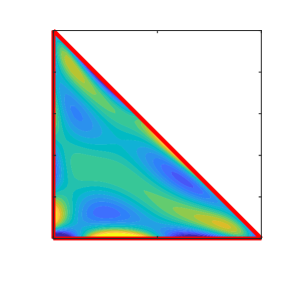
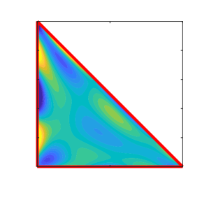
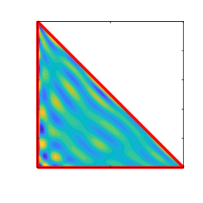
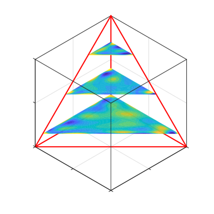
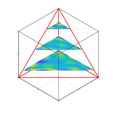
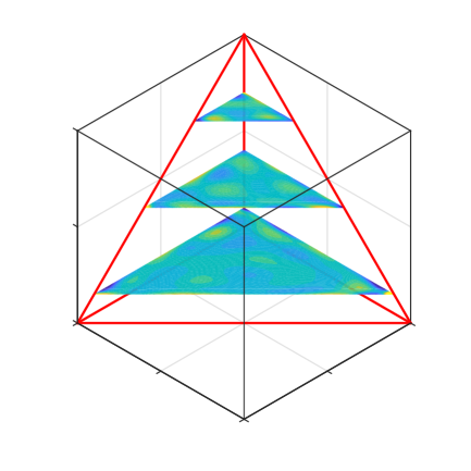
The contour plots of a few two- and three-dimensional divergence-free basis functions constructed in the reference element are shown in figure 3. Figures 3a and 3b show the $x$- and $y$-components, respectively, of a two-dimensional basis function of degree five. Figures 3c and 3d show the $x$- and $y$-components, respectively, of another two-dimensional basis function of degree 15. The $x$-, $y-$, and $z$-components of a three-dimensional basis function of degree 10 are shown in figures 3e, 3f, and 3g, respectively. Their slices at a few $z$-locations are shown.

(a)

(b)

(c)

Figure 4: Divergence-free projection in a general triangle. (a) Projection error v/s polynomial degree ($\circ$ - $x$-component and $\times$ - $y$-component). (b) Constraint error v/s polynomial degree. (c) Contours of the $x$-component of the projected velocity field for polynomial degree $20$.

4.3 Example divergence-free projection in a general triangle

In this example, we project the divergence-free velocity field $\bm{u}(x,y)=(\sin(\pi x)\cos(\pi y),-\cos(\pi x)\sin(\pi y))$ (Taylor-Green velocity field) onto the divergence-free basis constructed in a general triangle. The node-coordinate matrix of the triangle is $X^{(e)}=[0\hskip 5.0pt0;1\hskip 5.0pt0.8;0\hskip 5.0pt0.1]$. The MATLAB code used to perform the projection is given below:

k=20;d=2;Xe=[0 0;1 0.8;0.1 1];
tgfac=pi;ffu=@(x,y)sin(tgfac*x).*cos(tgfac*y);ffv=@(x,y)-cos(tgfac*x).*sin(tgfac*y);
[N,Q,H,Qd,x,w,~,C]=ardivfreebfref(k,d);
[Ne,Qde]=ardivfreebfgen(k,d,Xe,N,Q);
kp1d=(k+1)^d;xe=repmat(Xe(1,:),size(x(:,1)));xe=xe+x*(Xe(2:d+1,:)-repmat(Xe(1,:),[d 1]));
f=[ffu(xe(:,1),xe(:,2)); ffv(xe(:,1),xe(:,2))];
wd=repmat(w,[d 1]);wf=factorial(d);
dc=mgs_with_reorth(Qde,f,wd,wf,size(Qde,2),1);

Here, mgs_with_reorth is the function in figure 14 and dc is the vector storing the coefficients of the projection. The error in projection and in the satisfaction of the divergence-free constraint are computed using the below MATLAB code.

nplt=50;npltd=nplt^d;s1{1}=linspace(0,1,nplt); for j=2:d, s1{j}=s1{1}; end;
[st{1:d}]=ndgrid(s1{:}); s=reshape(cat(d,st{:}),[npltd d]);
s=[s(:,1) s(:,2:d).*cumprod(1-s(:,1:d-1),2)];
[Wde,W]=ardivfreebfeval(k,d,H,Ne,s);
se=repmat(Xe(1,:),size(s(:,1)));se=se+s*(Xe(2:d+1,:)-repmat(Xe(1,:),[d 1]));
fex=[ffu(se(:,1),se(:,2)) ffv(se(:,1),se(:,2))];
for i=1:d, err{i}=[]; end; yy=zeros(d*npltd,1);jdimp=0;jddimp=0;
errdiv=[0];kdim=nchoosek(k+d,d);
Xet=Xe’; Fe=Xet(:,2:d+1)-repmat(Xet(:,1),[1 d]); clear Xet;
Feinv=kron(inv(Fe),speye(nchoosek(k+d,d))); Ce=C*Feinv;
for j=0:k
  jdim=nchoosek(j+d,d); jddim=d*jdim-jdimp;
  yy=yy+Wde(:,jddimp+1:jddim)*dc(jddimp+1:jddim);
  for i=1:d
    err{i}=[err{i} max(abs(yy((i-1)*npltd+1:i*npltd)-fex(:,i)))];
  end
  ii=[]; for i=1:d, ii=[ii (i-1)*kdim+1:(i-1)*kdim+jdim]; end
  errdiv=[errdiv max(abs(Ce(1:jdimp,ii)*Ne(ii,1:jddim)*dc(1:jddim)))];
  jdimp=jdim;jddimp=jddim;
end

The projection error is defined to be the maximum absolute difference between $\bm{u}$ and the projection $\bm{u}_{h}$ evaluated at 2500 points in the triangle. The constraint error is defined for polynomial degree $j$ as the maximum absolute projection of the divergence of $\bm{u}_{h}$ along the orthonormal polynomials of degree less than $j$ ( $\max_{1\leq j^{\prime}\leq C_{d}^{j-1+d}}|\int_{\Omega^{(e)}}q_{j^{\prime}}\bm{\nabla}\cdot\bm{u}_{h}\,d\Omega|$).

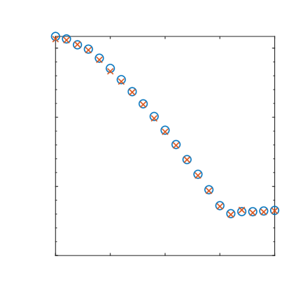
Figures 4a and 4b show the computed error in projection and in the satisfaction of the integral divergence-free constraint, respectively, as a function of polynomial degree. The projection error decreases exponentially with increasing polynomial degree and reaches machine precision for degree 19. The integral divergence-free constraint is satisfied up to machine precision for all polynomial degrees. The contours of the $x$-component of the projected vector computed with $k=20$ are shown in figure 4c.

Note that the coefficients of projection (stored in the vector dc) are computed only for polynomial degree 20. Since the constructed basis functions are hierarchical, the coefficients for degree $j$ less than 20 are nothing but the first $dC_{d}^{j+d}-C_{d}^{j-1+d}$ entries of the vector dc. Therefore, the projected function yy is incrementally computed at the points s for each polynomial degree j as yy=yy+Wde(:,jddimp+1:jddim)*dc(jddimp+1:jddim).

4.4 Computational cost

The computational cost to generate the divergence-free basis functions in the reference element (step 1) scales as $O((k+1)^{3d})$. The cost to construct the basis functions function in a general element (step 2) also scales as $O((k+1)^{3d})$, thought with a much smaller constant. The cost of evaluating the basis functions at $n_{p}$ points with ardivfreebfeval scales as $O(n_{p}(k+1)^{2d})$.

The most expensive part in the construction is step 1. However, we note that step 1 needs to be performed just once for the largest polynomial degree of interest, say $k$. The basis functions for degrees smaller than $k$ are part of the degree $k$ basis because of the hierarchy of the basis functions. The outputs of step 1 can even be precomputed and stored in a file that can be read at the beginning of each simulation. We note that step 2, which needs to be performed for each element in the mesh, is substantially cheaper than step 1. For example, for polynomial degree 15 in three dimensions, step 1 takes 20 seconds, while step 2 consumes just 0.3 seconds. Therefore, our methodology is a computationally efficient procedure to compute an orthonormal and hierarchical divergence-free basis for multiple elements.

4.5 On the structure of matrices $N$, $N^{(e)}$, and $H$

(a)

(b)

Figure 5: (a) Sparsity of $N$ and $N^{(e)}$. (b) Sparsity of $H$ with entries smaller than $10^{-13}$ neglected.

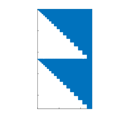
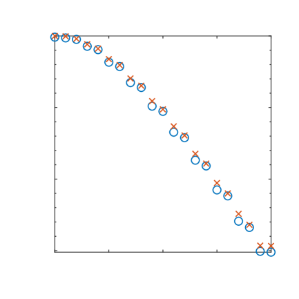
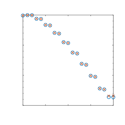
Nearly half of the entries in the coefficient matrices $N$ and $N^{(e)}$ are zeros and their non-zero (sparsity) patterns are identical. Consider the expression for the divergence-free basis functions $\bm{\varphi}_{\ell}$ and $\bm{\varphi}_{\ell}^{(e)}$ of degree $j$: $\bm{\varphi}_{\ell}=\sum_{i=1}^{d}\sum_{r=1}^{p_{j}}N_{(i-1)p+r,\ell}q_{r}\bm{e}_{i}$ and $\bm{\varphi}_{\ell}^{(e)}=\sum_{i=1}^{d}\sum_{r=1}^{p_{j}}N_{(i-1)p+r,\ell}^{(e)}q_{r}\left(\bm{x}\left(\bm{x}^{(e)}\right)\right)\bm{e}_{i}$, where $\ell=n_{j-1}+1,\dots,n_{j}$. Notice that the summation along $r$ is from $1$ to $p_{j}$ and not from $1$ to $p$, and therefore, the corresponding entries in matrices $N$ and $N^{(e)}$ are zeros. Specifically, $N_{(i-1)p+r,\ell}=0$ and $N_{(i-1)p+r,\ell}^{(e)}=0$ for $r$ larger than $p_{j}$ but less than or equal to $p$ and for each $i=1,\dots,d$. This non-zero pattern of $N$ and $N^{(e)}$ are shown in figure 5a. The matrices computed for the divergence-free projection problem discussed previously are used to plot this figure. Notice the staircase pattern of the matrices. This non-zero pattern can be used to reduce the cost of multiplying vectors with the matrices $N$ and $N^{(e)}$.

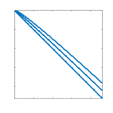
The structure of the upper-Hessenberg matrix $H$ generated using the Arnoldi-based procedure is very interesting. Several of its entries in the upper triangular portion are very close to zero. To show this, we define $H_{z}$ to be the matrix which is same as $H$ except that the entries in $H$ that are smaller than $10^{-13}$ are set to zero in $H_{z}$. Figure 5b shows the sparsity of $H_{z}$ for polynomial degree 20 in two dimensions. The sparsity pattern has three diverging bands comprising of block matrices. This is not accidental. It is a multi-dimensional analogue of the three-term recurrence relation of the one-dimensional orthonormal polynomials. One might be tempted to exploit this pattern to develop an Arnoldi-based process that would cost $O(k+1)^{2d}$ number of operations instead of the current $O(k+1)^{3d}$ cost. We developed one such method. But the algorithm was numerically unstable. The generated polynomials lost orthogonality. This is because of the same reason the Lanczos vectors lose orthogonality in finite-precision arithmetic without selective or complete reorthogonalization (Saad, 2011). Note that in the Arnoldi-based process in step 1, each vector $q_{j}$ is made orthogonal to all previous vectors $q_{1},\dots,q_{j-1}$. This is essentially complete reorthogonalization and it is necessary to retain orthogonality of the vectors $q_{j}$.

5 Applications

We use the constructed divergence-free basis functions to compute numerical solutions of some PDEs. For the first application, we show in detail how to exploit the orthonormal and hierarchical features of our basis. An efficient implementation of the hybridized mixed method is presented to compute numerical solutions for all polynomial degrees from zero to a given $k$. For the remaining applications, just the results are presented. Efficient implementations can be constructed similarly.

5.1 Helmholtz projection

The problem is as follows: Consider a domain $\Omega$. Let $T_{h}$ denote a triangulation of this domain. Given a function $\bm{g}$, compute its projection onto the divergence-free basis constructed in each element of the triangulation such that the normal component of the projection is continuous across the inter-element boundaries. This problems amounts to solving the below Helmholtz-type PDE problem:

$$\bm{u}\quad+ \bm{\nabla}\lambda =\bm{g} \quad\text{ in }\Omega,$$ (1)

$$\bm{\nabla}\cdot\bm{u} =0 \quad\text{ in }\Omega,\text{ and}$$

$$\lambda =0 \quad\text{ on }\partial\Omega.$$

Here, $\bm{u}$ is the desired projection, $\partial\Omega$ is the boundary of $\Omega$, and $\lambda$ is the Lagrange multiplier that imposes the divergence-free condition on $\bm{u}$. These equations are solved using the hybridized BDM mixed method (Brezzi et al., 1985) with one modification. The proposed divergence-free basis is used in place of the usual polynomial basis to approximate $\bm{u}$ in each element.

In the usual hyridized BDM mixed method for the above problem, $\bm{u}$ and $\lambda$ are approximated in each element $e$ by a polynomial of degree less than or equal to $k$ and $k-1$, respectively. Denote these approximations by $\bm{u}_{h}^{(e)}$ and $\lambda_{h}^{(e)}$. On each interior face $f$ of the mesh, the continuity of the normal component of the discontinuous approximation $\bm{u}_{h}^{(e)}$ is enforced using a Lagrange multiplier $\widehat{\lambda}^{(f)}_{h}$. This Lagrange multiplier is taken to be a polynomial of degree less than or equal $k$ on each face $f$ and is an approximation to $\lambda$ on the faces. In each element $e$, $\bm{u}_{h}^{(e)}$ and $\lambda_{h}^{(e)}$ are defined to be solution to the problem:

$$\int_{\Omega^{(e)}}{\bm{u}_{h}^{(e)}}\cdot{\bm{v}}\,d\Omega -\int_{\Omega^{(e)}}\lambda_{h}^{(e)}\bm{\nabla}\cdot\bm{v}\,d\Omega =\int_{\Omega^{(e)}}{\bm{g}}\cdot{\bm{v}}\,d\Omega-\sum_{f\in F(e)}\int_{\Gamma^{(f)}}\widehat{\lambda}_{h}^{(f)}\bm{v}\cdot\bm{n}\,d\Gamma \quad\forall\bm{v}\in[P_{k}(\Omega^{(e)})]^{d},$$ (2)

$$\int_{\Omega^{(e)}}w\bm{\nabla}\cdot\bm{u}_{h}^{(e)}\,d\Omega =0 \quad\forall w\in P_{k-1}(\Omega^{(e)}),$$

for each element $e$. Here, $\bm{v}$ and $w$ are test functions, $F(e)$ is the set of faces of element $e$, and $\Gamma^{(f)}$ is the domain of face $f$. The equations for the Lagrange multiplier $\widehat{\lambda}_{h}^{(f)}$ are the normal continuity constraints:

$$\int_{\Gamma^{(f)}}\left(\bm{u}_{h}^{(e^{+})}\cdot\bm{n}^{+}+\bm{u}_{h}^{(e^{-})}\cdot\bm{n}^{-}\right)\mu\,d\Gamma=0\quad\forall\mu\in P_{k}(\Gamma^{(f)}),$$ (3)

for each interior face $f$ of the mesh. Here, $e^{+}$ and $e^{-}$ are elements adjacent to face $f$. $\bm{n}^{+}$ and $\bm{n}^{-}$ are unit vectors normal to face $f$ and outward to the elements $e^{+}$ and $e^{-}$, respectively. On the boundary faces $f$, $\widehat{\lambda}_{h}^{(f)}$ is set to zero in accordance with the boundary condition.

Note that $\bm{u}_{h}^{(e)}$ is divergence-free at each point in the element $e$ because $\bm{\nabla}\cdot[P_{k}(\Omega^{(e)})]^{d}=P_{k-1}(\Omega^{(e)})$. Therefore, instead of approximating $\bm{u}_{h}^{(e)}$ with polynomials of degree less than or equal to $k$, it can be approximated with divergence-free polynomials of degree less than or equal to $k$. This simplifies (Cockburn, 2009) equation 2 to the below projection problem:

$$\int_{\Omega^{(e)}}{\bm{u}_{h}^{(e)}}\cdot{\bm{v}}\,d\Omega =\int_{\Omega^{(e)}}{\bm{g}}\cdot{\bm{v}}\,d\Omega-\sum_{f\in F(e)}\int_{\Gamma^{(f)}}\widehat{\lambda}_{h}^{(f)}\bm{v}\cdot\bm{n}\,d\Gamma \quad\forall\bm{v}\in\bm{V}_{k}(\Omega^{(e)}),$$ (4)

where $\bm{V}_{k}(\Omega^{(e)})$ is the set of all divergence-free polynomials of degree less than or equal to $k$ in element $e$. Note that $\lambda_{h}^{(e)}$ has disappeared from the equation because $\bm{\nabla}\cdot\bm{v}=0$ for all test functions $\bm{v}$ in $\bm{V}_{k}(\Omega^{(e)})$. To obtain an equation for just $\widehat{\lambda}^{(f)}$, following Cockburn (2016), we decompose $\bm{u}_{h}^{(e)}$ as $\bm{u}^{(e)}_{h}=\bm{u}^{(e)}_{\bm{g}}+\bm{u}^{(e)}_{\widehat{\lambda}_{h}}$, where $\bm{u}^{(e)}_{\bm{g}}$ and $\bm{u}^{(e)}_{\widehat{\lambda}_{h}}$ are defined as solutions to the problems:

$$\int_{\Omega^{(e)}}{\bm{u}_{\bm{g}}^{(e)}}\cdot{\bm{v}}\,d\Omega =\int_{\Omega^{(e)}}{\bm{g}}\cdot{\bm{v}}\,d\Omega \quad\forall\bm{v}\in\bm{V}_{k}(\Omega^{(e)}),\text{ and}$$ (5)

$$\bm{u}_{\widehat{\lambda}_{h}}^{(e)}=\sum_{f\in F(e)}\bm{u}_{\widehat{\lambda}^{(f)}_{h}}^{(e)},\text{ where }\int_{\Omega^{(e)}}{\bm{u}_{\widehat{\lambda}_{h}^{(f)}}^{(e)}}\cdot{\bm{v}}\,d\Omega =-\int_{\Gamma^{(f)}}\widehat{\lambda}_{h}^{(f)}\bm{v}\cdot\bm{n}\,d\Gamma \quad\forall\bm{v}\in\bm{V}_{k}(\Omega^{(e)}),$$ (6)

respectively. Then, we substitute them into equation 3 and this yields the below desired equation for just $\widehat{\lambda}_{h}^{(f)}$:

$$\begin{split}\sum_{e\in\{e^{+},e^{-}\}}\sum_{f^{\prime}\in F(e)}\int_{\Omega^{(e)}}{\bm{u}^{(e)}_{\widehat{\lambda}^{(f^{\prime})}_{h}}}\cdot{\bm{u}^{(e)}_{\mu}}\,d\Omega=-\sum_{e\in\{e^{+},e^{-}\}}\int_{\Omega^{(e)}}{\bm{u}^{(e)}_{\bm{g}}}\cdot{\bm{u}^{(e)}_{\mu}}\,d\Omega\quad\forall\mu\in P_{k}(\Gamma^{(f)}).\end{split}$$ (7)

To obtain the corresponding matrix problems, we expand $\bm{u}^{(e)}_{\bm{g}}$ and $\bm{u}^{(e)}_{\widehat{\lambda}_{h}^{(f)}}$ in terms of the divergence-free basis functions constructed in each element $e$ and expand $\widehat{\lambda}_{h}^{(f)}$ on each face $f$ in terms of the Arnoldi-based orthonormal polynomials constructed in the reference face element:

$$\widehat{\lambda}_{h}^{(f)}=\sum_{j=1}^{\widetilde{m}}c_{j}^{(f)}q_{j}^{(f)},\,\bm{u}_{\bm{g}}^{(e)}=\sum_{\ell=1}^{n}\alpha^{(e)}_{\ell}\bm{\varphi}^{(e)}_{\ell},\,\bm{u}_{\widehat{\lambda}_{h}^{(f)}}^{(e)}=\sum_{j=1}^{\widetilde{m}}c_{j}^{(f)}\bm{u}_{q_{j}^{(f)}}^{(e)},$$ (8)

where $\widetilde{m}$ is the dimension of $P_{k}(\Gamma^{(f)})$ (which equals $C_{d-1}^{k+d-1}$), and $\bm{u}_{q_{j}^{(f)}}^{(e)}=\sum_{\ell=1}^{n}\beta^{(e,f)}_{\ell,j}\bm{\varphi}^{(e)}_{\ell}$ is the solution to equation 6 with $\widehat{\lambda}_{h}^{(f)}$ set to $q_{j}^{(f)}$, i.e.,

$$\int_{\Omega^{(e)}}{\bm{u}_{q_{j}^{(f)}}^{(e)}}\cdot{\bm{v}}\,d\Omega =-\int_{\Gamma^{(f)}}q_{j}^{(f)}\bm{v}\cdot\bm{n}\,d\Gamma \quad\forall\bm{v}\in\bm{V}_{k}(\Omega^{(e)}),$$ (9)

and $c_{j}^{(f)}$, $\alpha^{(e)}_{\ell}$ and $\beta^{(e,f)}_{\ell,j}$ are the coefficients. Substituting the expressions for $\bm{u}_{\bm{g}}^{(e)}$ and $\bm{u}_{q_{j}^{(f)}}^{(e)}$ in equations 5 and 9, respectively, and requiring the equality for the test function $\bm{v}$ equal to each divergence-free basis function results in the below matrix problems for the coefficients $\alpha^{(e)}_{\ell}$ and $\beta^{(e,f)}_{\ell,j}$:

$$\sum_{\ell=1}^{n}\left(\int_{\Omega^{(e)}}{\bm{\varphi}^{(e)}_{\ell}}\cdot{\bm{\varphi}^{(e)}_{i}}\,d\Omega\right)\alpha_{\ell}^{(e)} =\int_{\Omega^{(e)}}{\bm{g}}\cdot{\bm{\varphi}_{i}^{(e)}}\,d\Omega \quad\text{for }i=1,\dots,n,\text{ and}$$ (10)

$$\sum_{\ell=1}^{n}\left(\int_{\Omega^{(e)}}{\bm{\varphi}^{(e)}_{\ell}}\cdot{\bm{\varphi}^{(e)}_{i}}\,d\Omega\right)\beta^{(e,f)}_{\ell,j} =-\int_{\Gamma^{(f)}}q_{j}^{(f)}\bm{\varphi}^{(e)}_{i}\cdot\bm{n}\,d\Gamma \quad\text{for }i=1,\dots,n;j=1,\dots,\widetilde{m};\text{ and }\forall f\in F(e).$$ (11)

The above two problems are called the local problems. They need to be solved in each element of the mesh. Substituting the expression for $\bm{u}_{\widehat{\lambda}_{h}^{(f)}}^{(e)}$ in equation 7 and requiring the equality for $\mu$ equal to each orthonormal polynomial yields the below equations for the coefficients $c_{j}^{(f)}$

$$\begin{split}\sum_{e\in\{e^{+},e^{-}\}}\sum_{f^{\prime}\in F(e)}\sum_{j=1}^{\widetilde{m}}\left(\int_{\Omega^{(e)}}{\bm{u}^{(e)}_{q_{j}^{(f^{\prime})}}}\cdot{\bm{u}^{(e)}_{q_{i}^{(f)}}}\,d\Omega\right)c_{j}^{(f^{\prime})}=-\sum_{e\in\{e^{+},e^{-}\}}\int_{\Omega^{(e)}}{\bm{u}^{(e)}_{\bm{g}}}\cdot{\bm{u}^{(e)}_{q_{i}^{(f)}}}\,d\Omega,\end{split}$$ (12)

for $i=1,\dots,\widetilde{m}$ and for each interior face $f$ of the mesh. The above problem is called the global problem. It couples the individual local problems.

The orthonormality and hierarchial features of the basis functions simplfy the local problem solution and the global problem assembly. Since the proposed basis functions $\bm{\varphi}_{\ell}^{(e)}$ are orthonormal, the local problems simplify to computing the below inner-products:

$$\alpha_{\ell}^{(e)} =\left(\int_{\Omega^{(e)}}{\bm{g}}\cdot{\bm{\varphi}_{\ell}^{(e)}}\,d\Omega\right)/|{\Omega^{(e)}}| \quad\text{for }\ell=1,\dots,n,\text{ and}$$ (13)

$$\beta^{(e,f)}_{\ell,j} =-\left(\int_{\Gamma^{(f)}}q_{j}^{(f)}\bm{\varphi}^{(e)}_{\ell}\cdot\bm{n}\,d\Gamma\right)/|{\Omega^{(e)}}| \quad\text{for }\ell=1,\dots,n;j=1,\dots,\widetilde{m};\text{ and }\forall f\in F(e).$$ (14)

Substituting the expression for $\bm{u}^{(e)}_{q_{i}^{(f)}}$ and using the orthogonality of the divergence-free basis functions $\bm{\varphi}_{\ell}^{(e)}$s simplifies the global problem to:

$$\begin{split}\sum_{e\in\{e^{+},e^{-}\}}\sum_{f^{\prime}\in F(e)}\sum_{j=1}^{\widetilde{m}}\left(\sum_{\ell=1}^{n}\beta^{(e,f^{\prime})}_{\ell,j}\beta^{(e,f)}_{\ell,i}|\Omega^{(e)}|\right)c_{j}^{(f^{\prime})}=-\sum_{e\in\{e^{+},e^{-}\}}\sum_{\ell=1}^{n}\alpha_{\ell}^{e}\beta^{(e,f)}_{\ell,i}|\Omega^{(e)}|,\end{split}$$ (15)

for $i=1,\dots,\widetilde{m}$ and for each interior face $f$ of the mesh. These equations can be written as the matrix problem $Ax=b$. Here, $A$ is the left-hand side matrix of size $n_{f}\widetilde{m}\times n_{f}\widetilde{m}$, where $n_{f}$ is the number of interior faces in the mesh. $x$ is the vector of coefficients of size $n_{f}\widetilde{m}\times 1$ and is defined as $x_{(f-1)\widetilde{m}+i}=c_{i}^{(f)}$. $b$ is the right-hand side vector of size $n_{f}\widetilde{m}\times 1$. The entries of the left-hand side matrix and the right-hand side vector are defined as:

$$A_{(f-1)\widetilde{m}+i,(f^{\prime}-1)\widetilde{m}+j}=\sum_{e\in\{e^{+},e^{-}\}}\sum_{\ell=1}^{n}\beta^{(e,f^{\prime})}_{\ell,j}\beta^{(e,f)}_{\ell,i}|\Omega^{(e)}|\text{ and }b_{(f-1)\widetilde{m}+i}=-\sum_{e\in\{e^{+},e^{-}\}}\sum_{\ell=1}^{n}\alpha_{\ell}^{(e)}\beta^{(e,f)}_{\ell,i}|\Omega^{(e)}|.$$

Note that the left-hand side matrix is sparse (Cockburn, 2016) because $A_{(f-1)\widetilde{m}+i,(f^{\prime}-1)\widetilde{m}+j}$ is non-zero if and only if the faces $f$ and $f^{\prime}$ belong to a common element.

The hierarchical feature of the basis functions can be exploited to develop an efficient assembly procedure for all polynomial degree from zero to $k$. The left-hand side matrix and the right-hand side vector are assembled using element matrix $A^{(e)}$ (size $(d+1)\widetilde{m}\times(d+1)\widetilde{m}$) and element vector $b^{(e)}$ (size $(d+1)\widetilde{m}\times 1$) that are computed for each element $e$ as:

$$\begin{split}A^{(e)}_{(g-1)\widetilde{m}+i,(g^{\prime}-1)\widetilde{m}+j}=\sum_{\ell=1}^{n}\beta^{(e,g^{\prime})}_{\ell,j}\beta^{(e,g)}_{\ell,i}|\Omega^{(e)}|\text{ and }b^{(e)}_{(g-1)\widetilde{m}+i}=\sum_{\ell=1}^{n}\alpha_{\ell}^{(e)}\beta^{(e,g)}_{\ell,i}|\Omega^{(e)}|.\end{split}$$ (16)

Here, $g$ and $g^{\prime}$ are the local index of the $(d+1)$ faces of the element. Since the basis functions are hierarchical, for each polynomial degree $k^{\prime}$ less than $k$, the element matrix $A^{(e,k^{\prime})}$ (size $(d+1)\widetilde{m}^{\prime}\times(d+1)\widetilde{m}^{\prime}$) and the element vector $b^{(e,k^{\prime})}$ (size $(d+1)\widetilde{m}^{\prime}\times 1$) are the following partial sums of the summations in the above equation:

$$\begin{split}A^{(e,k^{\prime})}_{(g-1)\widetilde{m}^{\prime}+i,(g^{\prime}-1)\widetilde{m}^{\prime}+j}=\sum_{\ell=1}^{n^{\prime}}\beta^{(e,g^{\prime})}_{\ell,j}\beta^{(e,g)}_{\ell,i}|\Omega^{(e)}|\text{ and }b^{(e)}_{(g-1)\widetilde{m}^{\prime}+i}=\sum_{\ell=1}^{n^{\prime}}\alpha_{\ell}^{(e)}\beta^{(e,g)}_{\ell,i}|\Omega^{(e)}|.\end{split}$$ (17)

where $n^{\prime}=dC_{d}^{k^{\prime}+d}-C_{d}^{k^{\prime}-1+d}$ and $\widetilde{m}^{\prime}=C_{d-1}^{k^{\prime}+d-1}$. Hence, given the coefficients $\beta_{\ell,j}^{(e,g)}$ and $\alpha_{\ell}^{(e)}$ that are computed for degree $k$, the element matrices and vectors for all degrees $k^{\prime}$ (up to $k$) can be incrementally constructed by performing an update to the element matrix and vector computed for degree $k^{\prime}-1$. Therefore, the left-hand side matrix $A^{(k^{\prime})}$ and the right-hand side vector $b^{(k^{\prime})}$ for all degrees $k^{\prime}$ (up to $k$) can also be incrementally assembled by updating the matrix $A^{(k^{\prime}-1)}$ and the vector $b^{(k^{\prime}-1)}$ computed for degree $k^{\prime}-1$. Using this idea, all the left-hand side matrices and the right-hand side vectors from polynomial degree $0$ to the given degree $k$ are efficiently constructed.

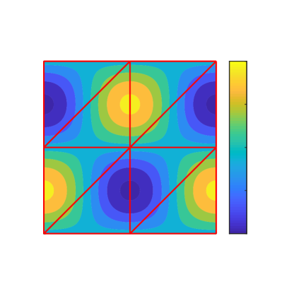
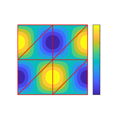
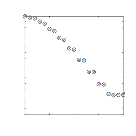
Consider $\Omega$ to be a unit square and the triangulation $T_{h}$ to be a uniform triangulation with eight elements. The triangulation is shown by the red lines in figure 6a. The function $\bm{g}$ is taken to be

$$(\cos(2\pi x)\sin(2\pi y)+0.1\cos(2\pi x)\sin(2\pi y),-\sin(2\pi x)\cos(2\pi y)+0.1\sin(2\pi x)\cos(2\pi y)).$$

For this $\bm{g}$, the exact solution $\bm{u}$ and $\lambda$ are

$$(\cos(2\pi x)\sin(2\pi y),-\sin(2\pi x)\cos(2\pi y)),\text{ and }\frac{0.1}{2\pi}\sin(2\pi x)\sin(2\pi y),$$

respectively. All numerical solutions from degree 0 to 20 are computed. The contours of the $x$-component of the numerical solution to $\bm{u}$ computed for polynomial degree $20$ are shown in figure 6a. Figure 6b shows the maximum error in the numerical solution to $\bm{u}$ as a function of polynomial degree. This error is the maximum absolute difference between $\bm{u}$ and its numerical solution evaluated at 1600 points in each element. The error decreases exponentially with increasing polynomial degree and reaches $10^{-14}$ for polynomial degree 20.

(a)

(b)

Figure 6: Helmholtz projection problem in unit square. (a) Mesh and contours of $x$-component of the numerical solution to $\bm{u}$ computed with polynomial degree 20. (b) Maximum absolute error in $x-$component $({\color[rgb]{0,0,1}\definecolor[named]{pgfstrokecolor}{rgb}{0,0,1}\circ})$ and $y-$component $({\color[rgb]{1,0,0}\definecolor[named]{pgfstrokecolor}{rgb}{1,0,0}\times})$ of the numerical solution to $\bm{u}$ v/s polynomial degree.

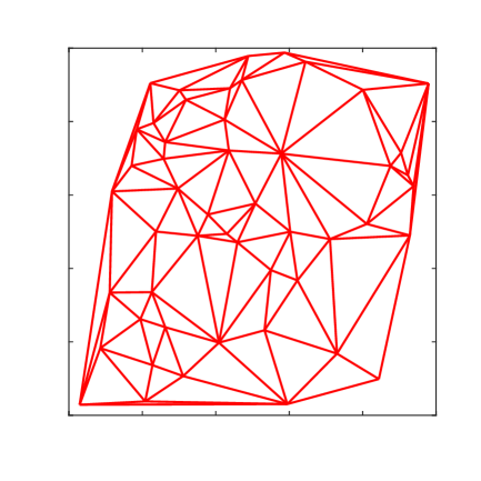
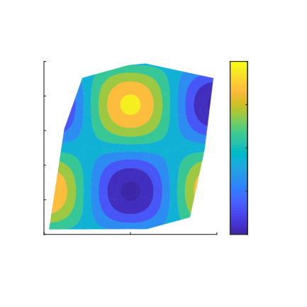
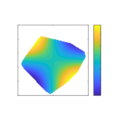
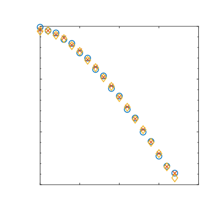
Consider $\Omega$ to be the convex hull of $50$ randomly scattered points in the unit square, and the triangulation $T_{h}$ to be a Delaunay triangulation of these points. The mesh is shown in figure 7a. The function $\bm{g}$ is taken to be $(\cos(2\pi x)\sin(2\pi y),-\sin(2\pi x)\cos(2\pi y))$. Since $\bm{g}$ is divergence-free, the exact solution $\bm{u}$ equals $\bm{g}$ and $\lambda$ equals zero. All numerical solutions from polynomial degree 0 to 20 are computed. The contours in figure 7b show the $x$-component of the numerical solution to $\bm{u}$ computed with polynomial degree 20. Figure 7c shows the maximum error in the numerical solution to $\bm{u}$ v/s polynomial degree. This error is the maximum absolute difference between $\bm{u}$ and its numerical solution evaluated at 1600 points in each element. The error decreases exponentially and stagnates at machine precision due to round-off error.

(a)

(b)

(c)

Figure 7: Helmholtz projection problem in a randomly generated two-dimensional domain. (a) Mesh. (b) $x$-component of the numerical solution to $\bm{u}$ computed with polynomial degree 20. (b) Maximum absolute error in $x-$component ($\color[rgb]{0,0,1}\definecolor[named]{pgfstrokecolor}{rgb}{0,0,1}\circ$) and $y-$component ($\color[rgb]{1,0,0}\definecolor[named]{pgfstrokecolor}{rgb}{1,0,0}\times$) of the numerical solution to $\bm{u}$ v/s polynomial degree.

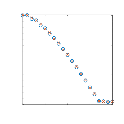
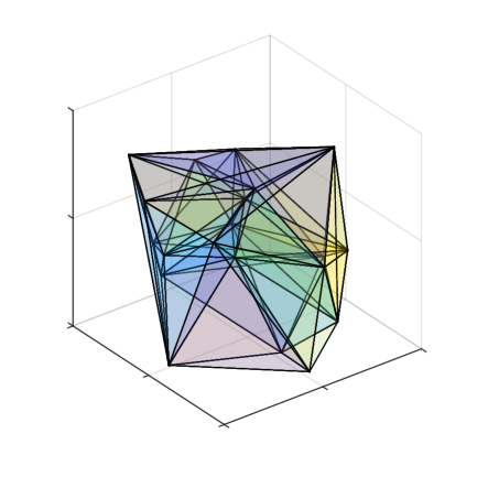
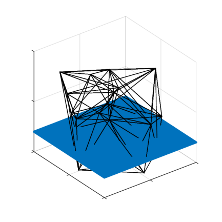
Consider $\Omega$ to be the three-dimensional convex hull of 20 randomly scattered points in the unit cube and $T_{h}$ to be a three-dimensional Delaunay triangulation of these points. The domain and the mesh are shown in the figure 8a. The function $\bm{g}$ is set to the three dimensional field

$$(\sin(\pi x)\cos(\pi y)\cos(\pi z),-0.5\cos(\pi x)\sin(\pi y)\cos(\pi z),-0.5\cos(\pi x)\cos(\pi y)\sin(\pi z)).$$

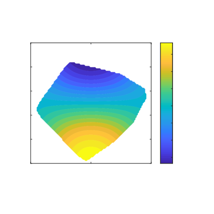
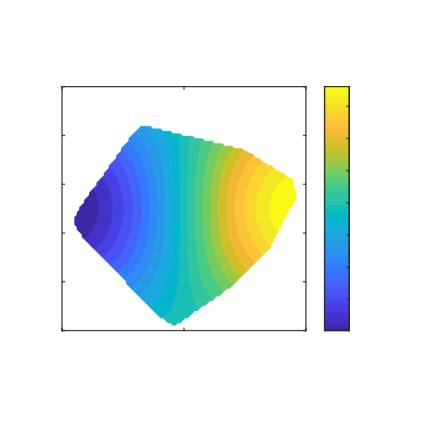
Since $\bm{g}$ is divergence-free, the exact solution $\bm{u}$ equals $\bm{g}$ and $\lambda$ equals zero. All numerical solutions up to polynomial degree 17 are computed. Figures 8b-d show the contours of $x-$, $y-$, and $z-$component of the numerical solution to $\bm{u}$ computed with polynomial degree 10 on a $x-y$ plane located at $z=0.2$ (plane is shown in figure 8e). Figure 8f shows the maximum error in the numerical solution to $\bm{u}$ v/s polynomial degree. This error is the maximum absolute different between $\bm{u}$ and its numerical solution evaluated at 8000 points in each element. The error decreases exponentially with polynomial degree up to machine epsilon.

(a)

(b)

(c)

(d)

(e)

(f)

Figure 8: Helmholtz projection problem in a randomly generated three dimensional domain. (a) Domain and mesh. (b) Location of z-slices. (c), (d), and (e) show the x-, y-, and z- component of the computed $\vec{u}_{h}$ on the z-slice. (f) Error in $x-$component ($\color[rgb]{0,0,1}\definecolor[named]{pgfstrokecolor}{rgb}{0,0,1}\circ$), $y-$component ($\color[rgb]{1,0,0}\definecolor[named]{pgfstrokecolor}{rgb}{1,0,0}\times$), and $z-$component ($\color[rgb]{1,.5,0}\definecolor[named]{pgfstrokecolor}{rgb}{1,.5,0}\diamond$) of the numerical solution to $\bm{u}$ v/s polynomial degree.

5.2 Laplace problem

The Laplace problem considered is: Given a domain $\Omega$, and the Dirichlet boundary data $\lambda_{D}$ on $\partial\Omega$, find $\bm{u}$ and $\lambda$ in $\Omega$ such that

$$\bm{u}\quad+ \bm{\nabla}\lambda =0 \quad\text{ in }\Omega$$ (18)

$$\bm{\nabla}\cdot\bm{u} =0 \quad\text{ in }\Omega$$

$$\lambda =\lambda_{D} \quad\text{ on }\partial\Omega.$$

Similar to the global divergence-free projection problem, i) we solve the above equation using our divergence-free basis in place of the usual polynomial basis to approximate $\bm{u}$ in the hybridized BDM mixed method (Brezzi et al., 1985), and ii) the left-hand side matrices and the right-hand side vectors for all polynomial degrees from 0 to the given degree $k$ are incrementally built.

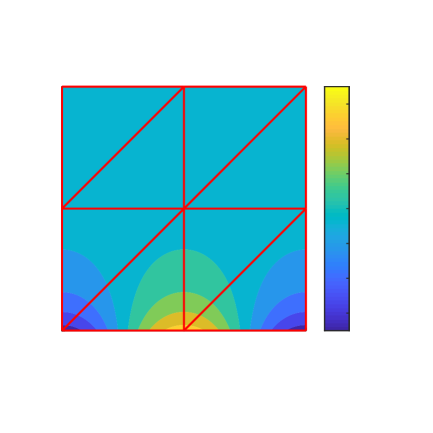
Consider $\Omega$ to be a unit square and its triangulation $T_{h}$ to be a uniform triangulation composed of eight elements. Figure 9a shows the mesh. The boundary data $\lambda_{D}$ is set using exact solution $\lambda=\sin(2\pi x)(\cosh(2\pi y)-\sinh(2\pi y))$. Contours of the $x$-component of the numerical solution to $\bm{u}$ computed with polynomial degree 20 are shown in figure 9a. Figure 9b shows the maximum error in the numerical solution to $\bm{u}$ v/s polynomial degree. This error is the maximum absolute difference between $\bm{u}$ and its numerical solution evaluated at 1600 points in each triangle. The error decreases exponentially with increasing polynomial degree. The error reaches $10^{-12}$ for degree 15 and then stagnates due to round-off error.

(a)

(b)

Figure 9: Laplace problem. (a) Mesh and $x-$ component of the numerical solution to $\bm{u}$ computed with polynomial degree 20. (b) Error in $x-$component ($\color[rgb]{0,0,1}\definecolor[named]{pgfstrokecolor}{rgb}{0,0,1}\circ$), and $y-$component ($\color[rgb]{1,0,0}\definecolor[named]{pgfstrokecolor}{rgb}{1,0,0}\times$) of the numerical solution to $\bm{u}$ v/s polynomial degree.

(a)

(b)

Figure 10: Poisson problem. (a) Mesh and $x-$component of the numerical solution to $\bm{u}$ computed with polynomial degree 20. (b) Error in $x-$component ($\color[rgb]{0,0,1}\definecolor[named]{pgfstrokecolor}{rgb}{0,0,1}\circ$), and $y-$component ($\color[rgb]{1,0,0}\definecolor[named]{pgfstrokecolor}{rgb}{1,0,0}\times$) of the numerical solution to $\bm{u}$ v/s polynomial degree.

Another Laplace problem considered is the corner singularity problem shown in figure 2 and its results were discussed in the introduction section. Some important results are reiterated. The numerical solution to $\lambda$ at the corner converges exponentially with increasing polynomial degree and is accurate up to twelve significant digits for polynomial degree eight. It takes just four seconds to compute all numerical solutions from polynomial degree zero to eight.

5.3 Poisson problem

The Poisson problem considered is: Given a domain $\Omega$ and a function $f$ in $\Omega$, find $\bm{u}$ and $\lambda$ such that

$$\bm{u}\quad+ \bm{\nabla}\lambda =0 \quad\text{ in }\Omega$$ (19)

$$\bm{\nabla}\cdot\bm{u} =f \quad\text{ in }\Omega$$

$$\lambda =0 \quad\text{ on }\partial\Omega.$$

The above equations are solved using the hybridized BDM mixed method. In each element of the mesh, we construct the divergence-free basis functions and use it to express the portion of $\bm{u}$ that depends on the unknown Lagrange multiplier on the element faces. For this problem, only the left-hand side matrix can be incrementally built for all polynomial degrees from zero to the prescribed degree $k$. The right-hand side vector needs to computed separately for each degree.

Consider $\Omega$ to be a unit square, and $T_{h}$ to be a uniform triangulation composed of eight elements. The mesh is shown in figure 10a. The data $f$ is computed assuming the exact solution $\lambda$ to be $\sin(2\pi x)\sin(2\pi y)$. Contours of the $x-$component of the numerical solution to $\bm{u}$ computed with polynomial degree 20 are shown in figure 10a. The error in the numerical solution to $\bm{u}$ is shown in figure 10b as a function of the polynomial degree. This error is maximum absolute difference between $\bm{u}$ and its numerical solution evaluated at 1600 points in each triangle. The error decreases exponentially with increasing polynomial degree. It reaches around $10^{-12}$ for degree 17 and then stagnates due to round-off error.

6 Summary

This paper develops a methodology to construct an orthonormal and hierarchical divergence-free polynomial basis in a simplex (triangles in 2D and tetrahedra in 3D) of arbitrary dimension. At the core of the construction is an Arnoldi-based procedure that constructs an orthonormal basis for polynomials of degree less than or equal to $k$ in $d$ dimensions. The generated basis is robust in finite-precision arithmetic. Using this basis in hybridized mixed methods leads to fast computation of all numerical solutions from polynomial degree zero to some given $k$. The orthonormality simplifies the local problem solution. The hierarchical feature allows the global (and element) matrices and vectors to be incrementally constructed for all degrees zero to $k$ using the local problem solution computed just for degree $k$. The constructed basis is applied to solve Helmholtz, Laplace and Poisson problem in smooth domains and in a domain with corner singularity. The basis can also be used for efficient numerical solution of other PDEs such as incompressible Stokes, incompressible Navier-Stokes, and Maxwell equations.

Appendix A The Arnoldi-based procedure generates a basis for polynomials

To show that the Arnoldi-based procedure generates a basis for polynomials, we can omit the orthogonalizations as they merely combine the polynomials without adding higher-degree polynomials. The polynomials generated with this omission are denoted by $m_{i}$. The algorithm with this omission is: $m_{1}=1$. For each degree $j=1,\dots,k$, compute the polynomials $m_{p_{j-1}+1},\dots,m_{p_{j}}$ of degree $j$ using the previously computed basis functions $m_{1},\dots,m_{p_{j-1}}$ and the algorithm given below:

1:Set $c=p_{j-1}$

2:for $i=1,\dots,d$ do

3:     $j^{\prime\prime}=C_{d-i}^{j-1+d-i}$

4:     for $j^{\prime}=1,\dots,j^{\prime\prime}$ do

5:         $m_{c+1}=\widehat{x}_{i}m_{p_{j-1}-j^{\prime\prime}+j^{\prime}}$

6:         $c=c+1$

7:     end for

8:end for

Figure 11: Illustration of the generation of monomials for $k=4$.

All it remains to prove is that the set of polynomials $m_{1},\dots,m_{p_{j}}$ form a basis for polynomials of degree less than or equal to $j$. In fact, the $m_{i}$s in this set are degree-ordered monomials of degree less than or equal to $j$. Furthermore, the above algorithm generates the monomials of degree $j$ using the monomials of degree $j-1$ and the coordinate operators. We visually show this for two dimensions $d=2$. Figure 11 shows the monomial generation process for $k=4$ and $d=2$ with the above algorithm. Here, we have used $x$ and $y$ in place of $x_{1}$ and $x_{2}$ for the sake of clarity. The red and blue arrows denote the action of the $x$-coordinate and $y$-coordinate operators, respectively. The circled numbers adjacent to each arrow shows the sequence in which the $m_{i}$s are generated. Each $m_{i}$ is equal to the monomial in parenthesis above or to the left of it. For degree $j$, the monomials are generated as $x^{j+1-r}y^{r}=\widehat{x}x^{j-r}y^{r}$ for $r=1,\dots,j$ and $y^{j+1}=\widehat{y}y^{j}$. Similarly, for arbitrary $d$, the monomials of degree $j$ are generated by applying the coordinate operators on the monomials of degree $j-1$. The first $C_{d-1}^{j-1+d-1}$ monomials of degree $j$ are generated by applying $\widehat{x}_{1}$ onto each monomial of degree $j-1$. The next $C_{d-2}^{j-1+d-2}$ monomials of degree $j$ are generated by applying the coordinate operator $\widehat{x}_{2}$ onto the last $C_{d-2}^{j-1+d-2}$ monomials of degree $j-1$, and so on.

Appendix B Step 1.2 generates an orthonormal basis for divergence-free polynomials

The set of divergence-free polynomials is a subset of the set of vector-valued polynomials. Therefore, each divergence-free basis function can be expanded in terms of the vector-valued polynomial basis $\{q_{r}\mathbf{e}_{i}\}$. The divergence-free polynomial basis function of degree $j$ is $\bm{\varphi}_{\ell}=\sum_{i=1}^{d}\sum_{r=1}^{p_{j}}N_{(i-1)p+r,\ell}q_{r}\bm{e}_{i}$. For degree $j$ and $j-1$, the number of divergence-free basis functions are $n_{j}$ and $n_{j-1}$, respectively. Therefore, the loop for degree $j$ should add $n_{j}-n_{j-1}$ functions, i.e., $\bm{\varphi}_{n_{j-1}+1},\dots,\bm{\varphi}_{n_{j}}$. These functions must be divergence-free. Hence, the divergence-free condition (i). The divergence of a degree $j$ vector-valued polynomial is another polynomial of degree $j-1$. The condition (i) is an integral condition that requires this degree $j-1$ polynomial to be zero. It does so by requiring its projection to be zero along each orthonormal polynomial $q_{i}$ of degree less than or equal to $j-1$. We use an integral condition for numerical stability reasons in the presence of finite-precision arithmetic. Using a pointwise imposition of the divergence-free constraint lead to large amplification of machine precision error at high polynomial degrees.

The dimension of the vector-valued polynomial basis $\{q_{r}\mathbf{e}_{i}\}$ for $r=1,\dots,p_{j}$ and $i=1,\dots,d$ is $dC_{d}^{j+d}$. The divergence-free condition imposes $C_{d}^{j-1+d}$ constraints. This gives us a total dimension of $n_{j}=dC_{d}^{j+d}-C_{d}^{j-1+d}$. To determine the new $n_{j}-n_{j-1}$ functions, we need certain other constraints. We require the new functions to have no component along the divergence-free basis funcitons of degree less than or equal to $j-1$, i.e., $\int_{\widehat{\Omega}}\bm{\varphi}_{\ell}\cdot\bm{\varphi}_{\ell^{\prime}}\,d\widehat{\Omega}=0$ for $\ell=n_{j-1}+1,\dots,n_{j}$ and $\ell^{\prime}=1,\dots,n_{j-1}$. Combining this with the requirement that the new $n_{j}-n_{j-1}$ must be orthonormal amongst each other yields condition (ii). Lastly, we would not want the new basis functions to be linearly dependent which would reduce the total dimension from being equal to $n_{j}$. Hence, we have condition (iii).

Appendix C Quadrature rule

(a)

(b)

Figure 12: (a) Quadrature points to exactly integrate a polynomial of degree 4 in the unit triangle. (b) Corresponding coordinates of the quadrature points in the unit square.

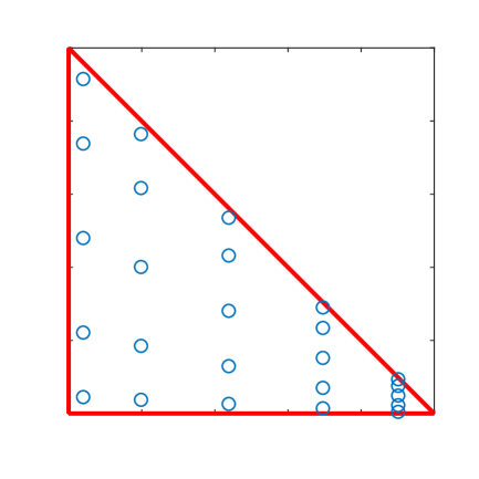
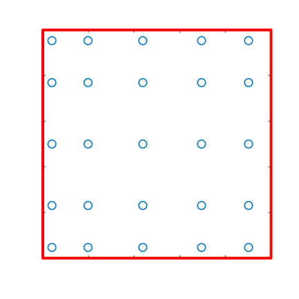
We first derive the quadrature rule for a unit triangle. Consider the following integral over a unit triangle: $g=\int_{0}^{1}\int_{0}^{1-x}f(x,y)\,dy\,dx$. Map the unit triangle to a unit square. Define $x=\zeta$ and $y=(1-\zeta)\eta$. Here, $(\zeta,\eta)$ is the coordinate of a point in the unit square, and $(x,y)$ is the image of this point in the unit triangle. The determinant of the Jacobian of this mapping is $(1-\zeta)$. Therefore, the integral transforms to $g=\int_{0}^{1}\int_{0}^{1}f(x(\zeta,\eta),y(\zeta,\eta))(1-\zeta)\,d\zeta\,d\eta$ in the unit square. Consider $f$ to be a polynomial of degree $2k$ in $x$ and $y$, then $f(x(\zeta,\eta),y(\zeta,\eta))$ is a polynomial in $\zeta$ and $\eta$ with each exponent less than or equal to $2k$. To integrate exactly along $\eta$, use $(k+1)$ Gauss-Legendre quadrature points along $\eta$. Along $\zeta$, note that there is the weight $(1-\zeta)$. Therefore, to integral exactly along $\zeta$, use $(k+1)$ Gauss-Jacobi points that correspond to the weight $(1-\zeta)$. Therefore, the quadrature rule to exactly integrate a polynomial of degree $2k$ is $\sum_{i=1}^{k+1}\sum_{j=1}^{k+1}f(x_{i,j},y_{i,j})w_{i,j}$. Here, $x_{i,j}=\zeta_{i}$, $y_{i,j}=(1-\zeta_{i})\eta_{j}$, and $w_{i,j}=w_{i}^{\zeta}w_{j}^{\eta}$. $\{\zeta_{i}\}_{i=1}^{k+1}$ and $\{w_{i}^{\zeta}\}_{i=1}^{k+1}$ are the Gauss-Jacobi quadrature points and weights with the weight function $(1-\zeta)$, respectively. $\{\eta_{i}\}_{i=1}^{k+1}$ and $\{w_{i}^{\eta}\}_{i=1}^{k+1}$ are the Gauss-Legendre quadrature points and weights, respectively. Figure 12a shows the quadrature points to exactly integrate a polynomial of degree 4 in the unit triangle. The corresponding points in the unit square are shown in figure 12b. Similarly, in arbitrary dimension $d$, the general integral over the unit simplex is:

$$g=\int_{0}^{1}\int_{0}^{1-x_{1}}\int_{0}^{1-x_{1}-x_{2}}\dots\int_{0}^{1-x_{1}-\dots-x_{d-1}}f\,dx_{d}\,\dots dx_{1}.$$

The mapping from the unit hypercube to the unit simplex $\bm{x}(\bm{\zeta})$ is:

$$x_{1}=\zeta_{1},\,x_{2}=(1-\zeta_{1})\zeta_{2},\dots,\,x_{d}=(1-\zeta_{1})\dots(1-\zeta_{d-1})\zeta_{d}.$$

The transformed integral is:

$$g=\int_{0}^{1}\dots\int_{0}^{1}f(\bm{x}(\bm{\zeta}))(1-\zeta_{1})^{(d-1)}\dots(1-\zeta_{d-1})\,d\zeta_{d}\,\dots d\zeta_{1}.$$

The quadrature rule is:

$$g=\sum_{i_{1}=1}^{k+1}\dots\sum_{i_{d}=1}^{k+1}f(x_{1_{i_{1},\dots,i_{d}}},\dots,x_{d_{i_{1},\dots,i_{d}}})w_{i_{1},\dots,i_{d}}.$$

Here, the quadrature point $\bm{x}_{i_{1},\dots,i_{d}}=\bm{x}(\zeta_{1_{i_{1}}},\dots,\zeta_{d_{i_{d}}})$ and $\{\zeta_{j_{i}}\}_{i=1}^{k+1}$ are the Gauss-Jacobi quadrature points with weight function $(1-\zeta_{j})^{d-j}$. The quadrature weight $w_{i_{1},\dots,i_{d}}=w_{1_{i_{1}}}\dots w_{d_{i_{d}}}$, where $\{w_{j_{i}}\}_{i=1}^{k+1}$ are the corresponding Gauss-Jacobi quadrature weights along the $j^{th}$ dimension. The quadrature points and weights are rearranged into a matrix $x$ and a vector $w$, respectively. $x$ is a matrix of size $(k+1)^{d}\times d$. The $i^{th}$ component of the coordinate vector of each point is stored in the $i^{th}$ column of $x$. $w$ is a vector of size $(k+1)^{d}$.

Appendix D Construction of derivative matrices

The derivative matrices yield the partial derivative of the function at the quadrature points using the values of the function at the same points. We first derive these matrices for two dimensions. Observe that in the unit square (figure 12b), the quadrature points form a Cartesian grid. The derivative matrices for this Cartesian grid can be computed using the one-dimensional derivative matrices and taking its kronecker tensor product with the identity matrix. The derivative matrix in the unit triangle can then be obtained using the chain rule: $\partial f/\partial x=\partial f/\partial\zeta\partial\zeta/\partial x+\partial f/\partial\eta\partial\eta/\partial x$ and $\partial f/\partial y=\partial f/\partial\zeta\partial\zeta/\partial y+\partial f/\partial\eta\partial\eta/\partial y$. Denote the derivative matrix along the $\zeta$ direction by $DZ$. It is the kronecker tensor product $DZ=kron(I,DZ1)$. Here, $I$ is the $(k+1)\times(k+1)$ identity matrix and $DZ1$ is the one-dimensional differentiation matrix along $\zeta$. To construct $DZ1$, we use the barycentric Lagrange-based procedure of Berrut and Trefethen (2004). $DZ1$ is a $(k+1)\times(k+1)$ matrix given by $DZ1_{i,j}=(\lambda_{j}/\lambda_{i})1/(\zeta_{i}-\zeta_{j})$ for $i\neq j$ and $DZ1_{i,j}=-\sum_{i\neq j}DZ1_{i,j}$. Here, $\zeta_{i}$ is the $i^{th}$ quadrature point along the $\zeta$ direction. $\lambda_{i}$ is the $i^{th}$ barycentric weight given by $\lambda_{i}=1/\prod_{j\neq i}(\zeta_{i}-\zeta_{j})$. Similarly, the derivative matrix along $\eta$ direction can be constructed. It is $DN=kron(DN1,I)$, where $DN1$ is the one-dimensional differentiation matrix along $\eta$ given by $DN1_{i,j}=(\gamma_{j}/\gamma_{i})1/(\eta_{i}-\eta_{j})$ for $i\neq j$ and $DN1_{i,j}=-\sum_{i\neq j}DN1_{i,j}$. Here, $\eta_{i}$ is the $i^{th}$ quadrature point along the $\eta$ direction. $\gamma_{i}$ is the $i^{th}$ barycentric weight given by $\gamma_{i}=1/\prod_{j\neq i}(\eta_{i}-\eta_{j})$. In the unit simplex, the derivative matrices are then $DX=DZ+(y/(1-x)^{2}).^{*}DN$ and $DY=(1/(1-x)).^{*}DN$, where the $.^{*}$ operator follows the MATLAB notation.

This procedure to construct the derivative matrices can be extended to an arbitrary dimension $d$. Denote the matrix of quadrature points by $x$. Its size is $(k+1)^{d}\times d$. Let $\{\zeta^{(i)}_{j}\}_{j=1}^{k+1}$ denote the Gauss-Jacobi quadrature points in the unit hypercube along the $i^{th}$ direction. The algorithm is:

1:for $i=1,\dots,d$ do$\triangleright$ Barycentric weights

2:     for $j=1,\dots,k+1$ do

3:         $\lambda^{(i)}_{j}=1/\prod_{j\neq\ell}(\zeta^{(i)}_{j}-\zeta^{(i)}_{\ell})$

4:     end for

5:end for

6:for $i=1,\dots,d$ do$\triangleright$ One-dimensional derivative matrices in the unit hypercube

7:     for $m=1,\dots,k+1$ do

8:         for $n=1,\dots,k+1$ do

9:              if $m\neq n$ then

10:                  $DZ1^{(i)}_{m,n}=\lambda^{(i)}_{n}/\lambda^{(i)}_{m}1/(\zeta^{(i)}_{m}-\zeta^{(i)}_{n})$

11:              else

12:                  $DZ1^{(i)}_{m,m}=-\sum_{j=1,j\neq m}^{k+1}\lambda^{(i)}_{j}/\lambda^{(i)}_{m}1/(\zeta^{(i)}_{m}-\zeta^{(i)}_{j})$

13:              end if

14:         end for

15:     end for

16:end for

17:$DZ^{(1)}=DZ1^{(1)}$ $\triangleright$ Multi-dimensional derivative matrices in the unit hypercube

18:for $i=2,\dots,d$ do

19:     $DZ^{(i)}=eye(k+1)$

20:end for

21:for $i=1,\dots,d$ do

22:     for $j=2,\dots,d$ do

23:         if $j==i$ then

24:              $DZ^{(i)}=kron(DZ1^{(i)},DZ^{(i)})$

25:         else

26:              $DZ^{(i)}=kron(eye(k+1),DZ^{(i)})$

27:         end if

28:     end for

29:end for

30:$DX^{(1)}=DZ^{(1)}$ $\triangleright$ Transforming the derivative matrices from unit hypercube to unit simplex

31:for $i=2,\dots,d$ do

32:     $DX^{(i)}=zeros((k+1)^{d})$

33:end for

34:$tt1=ones((k+1)^{d})$

35:for $j=2,\dots,d$ do

36:     $tt1=tt1-x(:,j-1)$; $tt2=1./tt1$; $tt3=x(:,j)./tt1^{2}$

37:     for $i=1,\dots,j-1$ do

38:         $DX^{(i)}=DX^{(i)}+DZ^{(j)}.^{*}tt3$

39:     end for

40:     $DX^{(j)}=DX^{(j)}+DR^{(j)}.^{*}tt2$

41:end for

Appendix E Deriving the algorithm in section 3.1.2 from the algorithm in step 1.2 in section 2

Consider the three conditions in step 1.2 of section 2. Substituting the expression for $\bm{\varphi}_{\ell}$ into condition (i) yields

$$\sum_{i=1}^{d}\sum_{r=1}^{p_{j}}\left(\int_{\widehat{\Omega}}q_{s}\frac{\partial q_{r}}{\partial x_{i}}\,d\widehat{\Omega}\right)N_{(i-1)p+r,\ell}=0\text{ for }\ell=n_{j-1}+1,\dots,n_{j}\text{ and }s=1,\dots,p_{j-1}.$$

These are linear constraints imposed on $\{N_{(i-1)p+r,\ell}\}$. Define the coefficients of the constraint to be $C_{s,(i-1)p+r}=\left(\int_{\widehat{\Omega}}q_{s}\frac{\partial q_{r}}{\partial x_{i}}\,d\widehat{\Omega}\right)$. The coefficients $C_{s,(i-1)p+r}$ are stored in the divergence-free constraint matrix $C$. Using the orthonormality of the $q_{i}$s, condition (ii) can be shown to be equivalent to $\sum_{i=1}^{d}\sum_{r=1}^{p_{j}}N_{(i-1)p+r,\ell^{\prime}}N_{(i-1)p+r,\ell}=\delta_{\ell\ell^{\prime}}$ for $\ell=n_{j-1}+1,\dots,n_{j},\ell^{\prime}=1,\dots,n_{j}$. Since the $q_{i}$s are linearly independent, condition (iii) is equivalent to requiring the rank of the submatrix of $N$ formed by the $n_{j-1}+1$ to $n_{j}$ columns to be $n_{j}-n_{j-1}$. Computing the coefficients $\{N_{(i-1)p+r,\ell}\}$ that satisfy the above conditions for each polynomial degree $j$ is equivalent to finding an orthonormal basis for the null-space of the augmented matrix:

$$\begin{bmatrix}C_{1:p_{j-1},ii}\\ N^{T}_{ii,1:n_{j-1}}\end{bmatrix}.$$

Here, $ii$ is the index vector of column indices of $C$ (or row indices of $N$) that correspond to degree less than or equal to $j$ constructed as:

1:$ii=[]$

2:for $i=1,\dots,d$ do

3:     $ii=[ii,\,(i-1)p+1:(i-1)p+p_{j}]$

4:end for

Replacing symbolic polynomials with vectors storing its value at the quadrature points and continous inner-products with equivalent discrete inner-products yields the algorithm in 3.1.2.

Appendix F Deriving the algorithm in section 3.2.1 from the algorithm in step 2.1 in section 2

Using the orthonormality of the $q_{i}$s, condition (ii) simplifies to $\sum_{i=1}^{d}\sum_{r=1}^{p_{j}}N_{(i-1)p+r,\ell}^{(e)}N_{(i-1)p+r,\ell^{\prime}}^{(e)}=\delta_{\ell\ell^{\prime}}$ for $\ell$ and $\ell^{\prime}=n_{j-1}+1,\dots,n_{j}$. Since the $q_{i}$s are linearly independent, condition (iii) simplifies to enforcing the rank of the submatrix of $N^{(e)}$ formed by the columns from $n_{j-1}+1$ to $n_{j}$ to be $n_{j-1}-n_{j}$. To compute the coefficients that satisfy the divergence-free requirement in condition (i), we use the divergence-free basis functions $\bm{\varphi}_{n_{j-1}+1},\dots,\bm{\varphi}_{n_{j}}$ that were computed in the reference element. The expression for these functions in terms of the orthonormal polynomials is $\bm{\varphi}_{\ell}=\sum_{i=1}^{d}\sum_{r=1}^{p_{j}}N_{(i-1)p+r,\ell}q_{r}\bm{e}_{i},\text{ for }\ell=n_{j-1}+1,\dots,n_{j}$. The coefficients $N_{(i-1)p+r,\ell}$ were computed such that they satisfy the divergence-free condition in the reference element: $\sum_{i=1}^{d}\sum_{r=1}^{p_{j}}{\partial q_{r}}/{\partial x_{i}}N_{(i-1)p+r,\ell}=0$. The gradient ${\partial q_{r}}/{\partial x_{i}}$ in the reference element can be expanded in terms of the gradient in the current element as ${\partial q_{r}}/{\partial x_{i}}=\sum_{m=1}^{d}{\partial x_{m}^{(e)}}/{\partial x_{i}}{\partial q_{r}}/{\partial x_{m}^{(e)}}$. Substituting this into the divergence-free condition gives $\sum_{i=1}^{d}\sum_{r=1}^{p_{j}}\sum_{m=1}^{d}{\partial x_{m}^{(e)}}/{\partial x_{i}}{\partial q_{r}}/{\partial x_{m}^{(e)}}N_{(i-1)p+r,\ell}=0$. Swapping the order of summation over $i$ and $m$, and rearranging yields $\sum_{m=1}^{d}\sum_{r=1}^{p_{j}}\left[\sum_{i=1}^{d}{\partial x_{m}^{(e)}}/{\partial x_{i}}N_{(i-1)p+r,\ell}\right]{\partial q_{r}}/{\partial x_{m}^{(e)}}=0$. Interchanging the index $i$ to $m$ and $m$ to $i$ gives $\sum_{i=1}^{d}\sum_{r=1}^{p_{j}}\left[\sum_{m=1}^{d}{\partial x_{i}^{(e)}}/{\partial x_{m}}N_{(m-1)p+r,\ell}\right]{\partial q_{r}}/{\partial x_{i}^{(e)}}=0$. Comparing the above equation to the divergence-free condition (i), we deduce that setting $N_{(i-1)p+r,\ell}^{(e)}$ to a linear combination of the form $\sum_{\ell^{\prime}=n_{j-1}+1}^{n_{j}}A_{\ell^{\prime},\ell}\left[\sum_{m=1}^{d}{\partial x_{i}^{(e)}}/{\partial x_{m}}N_{(m-1)p+r,\ell^{\prime}}\right]$ will satisfy the divergence-free condition, for any set of coefficients $A_{\ell^{\prime},\ell}$ that form a full rank matrix $A_{n_{j-1}+1:n_{j},n_{j-1}+1:n_{j}}$. The coefficients $A_{\ell^{\prime},\ell}$ are implicitly chosen as follows such that the resulting $N_{(i-1)p+r,\ell}^{(e)}$s satisfy the orthonormality condition (ii). The linear combinations $\bar{N}_{(i-1)p_{j}+r,\ell}=\sum_{m=1}^{d}\partial x_{i}^{(e)}/\partial x_{m}N_{(m-1)p+r,\ell}$ are computed for $i=1,\dots,d$, $r=1,\dots,p_{j}$, and $\ell=n_{j-1}+1,\dots,n_{j}$. These linear combinations are orthogonalized against the previously computed coefficients $N_{(i-1)p+r,\ell}^{(e)}$ such that new $\bar{N}_{(i-1)p_{j}+r,\ell}$s satisfy $\sum_{i=1}^{d}\sum_{r=1}^{p_{j}}\bar{N}_{(i-1)p_{j}+r,\ell}N_{(i-1)p+r,\ell^{\prime}}^{(e)}=0$ for $\ell^{\prime}=1,\dots,n_{j-1}$. These $\bar{N}_{(i-1)p_{j}+r,\ell}$s are finally orthonormalized amongst each other to yield the required coefficients ${N}_{(i-1)p+r,\ell}^{(e)}$s that satisfy $\sum_{i=1}^{d}\sum_{r=1}^{p_{j}}{N}_{(i-1)p+r,\ell}^{(e)}N_{(i-1)p+r,\ell^{\prime}}^{(e)}=0$ for $\ell$ and $\ell^{\prime}$ equals $n_{j-1}+1,\dots,n_{j}$. The computed coefficients ${N}_{(i-1)p+r,\ell}^{(e)}$s also satisfy the rank requirement condition (iii) because the matrix formed by the linear combinations $\bar{N}_{(i-1)p_{j}+r,\ell}$s has rank $n_{j}-n_{j-1}$ and the subsequent orthogonalizations and orthonormalizations that yield the $n_{j-1}$ to $n_{j}$ columns of $N^{(e)}$ do not modify this rank. This yields the algorithm in section 3.2.1.

Appendix G Monomial divergence-free basis functions

Figure 13 shows the MATLAB code to construct the monomial divergence-free basis for arbitrary polynomial degree and spatial dimension.

⬇

1function [bf] = mondivfreebf(k,d)

2%%%% function [bf] = mondivfreebf(k,d)

3%%%% Inputs: k - polynomial degree, d - spatial dimension.

4%%%% Outputs: bf - function handle to the divergence-free basis funcitons.

5 sz=d*nchoosek(k+d,d)-nchoosek(k-1+d,d); alpha=zeros(d,sz); l=zeros(d,d,sz); t=0; bf=cell(sz,1);

6%%%%--------------------Loop over polynomial degree.

7 for ktil=0:k

8%%%%--------------------Construct monomial basis of homogeneous polynomials of degree ktil.

9 [talpha,tl]=divfree_subspace_of_ptilk(ktil,d); tsz=size(talpha,2);

10%%%%--------------------Get function handles.

11 for i=1:tsz, tta=talpha(:,i); ttl=tl(:,:,i); bf{t+i}=@(x)divfree_bf_gen_func(x,tta,ttl); end

12 t=t+tsz;

13 end

14function [alpha,l] = divfree_subspace_of_ptilk (k,d)

15 if(k==0), alpha=eye(d); l=zeros(d,d,d); return; end

16 szptilk=nchoosek(k+d-1,d-1); szptilkd=d*szptilk; szdivc=nchoosek(k+d-2,d-1); szdivptilkd=szptilkd-szdivc;

17 alpha=zeros(d,szdivptilkd); l=zeros(d,d,szdivptilkd);

18 mnptilk=monomials_of_ptilk(k,d); mnptilkm1=monomials_of_ptilk(k-1,d); eqnmapkm1=mnexp_to_eqnmap(mnptilkm1,k-1,d);

19 coeff=zeros(d,szdivc); idcoeff=zeros(d,szdivc); t=0;

20 for i=1:d

21 for n=1:szptilk

22 % Check for zero divergence.

23 tt1=mnptilk(i,n);

24 if(tt1==0), t=t+1; alpha(i,t)=1d0; l(:,i,t)=mnptilk(:,n);

25 else % We have non-zero divergence.

26 talpha=tt1; tl=mnptilk(:,n); tl(i)=tl(i)-1;

27 tl1d=mnexp_to_1d(tl,k-1,d); eqnno=eqnmapkm1(tl1d); coeff(i,eqnno)=talpha; idcoeff(i,eqnno)=n;

28 end

29 end

30 end

31 % Construct the remaining basis functions.

32 tt2=zeros(d-1,1);

33 for n=1:szdivc

34 % Solve for the first coefficient in terms of the remaining coefficients.

35 for i=1:d-1, tt2(i)=-coeff(i+1,n)/coeff(1,n); end

36 % Construct the remaining divergence-free basis functions using these monomials.

37 for i=2:d

38 t=t+1; alpha(1,t)=tt2(i-1); l(:,1,t)=mnptilk(:,idcoeff(1,n)); alpha(i,t)=1d0;

39 l(:,i,t)=mnptilk(:,idcoeff(i,n));

40 end

41 end

42function [v] = monomials_of_ptilk (k,d)

43 tmp=nchoosek(1:(k+d-1),d-1); tmp=tmp’; szptilk=size(tmp,2); v=zeros(d,szptilk);

44 for n=1:szptilk

45 v(1,n)=tmp(1,n)-1;

46 for i=2:d-1

47 v(i,n)=tmp(i,n)-tmp(i-1,n)-1;

48 end

49 v(d,n)=k+d-1-tmp(d-1,n);

50 end

51function [v] = mnexp_to_eqnmap (mn,k,d)

52 v=zeros((k+1)^d,1);

53 sz=size(mn,2);

54 for n=1:sz, tmp=mnexp_to_1d(mn(:,n),k,d); v(tmp)=n; end

55function [v] = mnexp_to_1d (mn,k,d)

56 v=mn(1)+1;

57 for i=2:d, v=v+(mn(i))*((k+1)^(i-1)); end

58function [bf] = divfree_bf_gen_func(x,talpha,tl)

59 [m n]=size(x); bf=zeros([m n]);

60 for i=1:n, bf(:,i)=talpha.*(prod(x(:,i).^tl(:,:))’); end

Figure 13: mondivfreebf.m - MATLAB code to construct the monomial divergence-free basis.

Appendix H MATLAB implementation of step 1

The MATLAB function ardivfreebfref in figure 14 shows our MATLAB implementation of step 1. The required quadrature points and weights are constructed in lines 9-12. Lines 31-38 show the operations of the Arnoldi-based process that correspond to the $j^{th}$ polynomial degree. The function GaussJacobi in line 9 is an external function that yields the one-dimensional quadrature points x1 and weights w1 for the $(k+1)$-point Gauss-Jacobi quadrature with weight function $(1-x)^{\texttt{d-i}}$ in the interval $[-1,+1]$. We use the GuassJacobi function from https://www.math.umd.edu/~petersd/460/GaussJacobi.m. Lines 14-23 show the construction of the derivative matrices DX{i} for i=1,...,d using the barycentric Lagrange interpolation-based procedure. Lines 40-45 show the computation of the columns of $N$ for each polynomial degree using the built-in null function in MATLAB. The null function computes the singular value decomposition of the input matrix in the background and sets the output to the right singular vectors of the matrix that have singular values close to machine epsilon.

⬇

1function [N,Q,H,Qd,x,w,x1,C,DX,D1,v1]=ardivfreebfref(k,d)

2%%%% function [N,Q,H,Qd,x,w,x1,C,DX,D1,v1]=ardivfreebfref(k,d)

3%%%% Inputs: k - Polynomial degree, d - Spatial dimension.

4%%%% Outputs: N - Coeff. matrix, Qd - Div. free poly. basis, Q - Poly. basis, H - Upper Hess. matrix,

5%%%% x - Int. pts, w - Int. wts, C - Div. matrix, DX - Der. matrix, D1 - 1d Der. matrix, v1 - Bary. wts.

6 kp1=k+1; kp1d=(kp1)^d; kdim=nchoosek(k+d,d); kdimp=nchoosek(k-1+d,d);

7 dkdim=d*kdim; kddim=dkdim-kdimp; wf=double(factorial(d)); hkdim=nchoosek(k+d-1,d-1);

8%%%%--------------------Quadrature rule.

9 for i=1:d, [x1{i},w1{i}]=GaussJacobi(kp1,0,d-i); x1{i}=0.5*(1+x1{i}); w1{i}=(0.5)^(d-i+1)*w1{i}; end

10 [xt{1:d}]=ndgrid(x1{:}); [wt{1:d}]=ndgrid(w1{:});

11 xt=reshape(cat(d,xt{:}),[kp1d d]); wt=reshape(cat(d,wt{:}),[kp1d d]);

12 x=[xt(:,1) xt(:,2:d).*cumprod(1-xt(:,1:d-1),2)]; w=prod(wt,2);clear xt wt;

13%%%%--------------------Derivative matrices.

14 for i=1:d, v1{i}=barywts(x1{i}); D1{i}=barydiff(x1{i},v1{i}); end

15 DR{1}=D1{1};for i=2:d, DR{i}=speye(kp1); end

16 for i=1:d,

17 for j=2:d, if(j==i), DR{i}=kron(D1{i},DR{i}); else, DR{i}=kron(speye(kp1),DR{i}); end; end

18 end

19 DX{1}=DR{1}; sz=size(DX{1}); for i=2:d, DX{i}=zeros(sz); end; tt1=ones(kp1d,1);

20 for j=2:d

21 tt1=tt1-x(:,j-1);tt2=1./tt1;tt3=x(:,j)./tt1.^2;

22 for i=1:j-1, DX{i}=DX{i}+DR{j}.*tt3; end; DX{j}=DX{j}+DR{j}.*tt2;

23 end

24%%%%--------------------Loop over polynomial degree.

25 N=zeros(dkdim,kddim); N([1:kdim:dkdim],[1:d])=eye(d); C=zeros(kdimp,dkdim); DXQ=zeros(kp1d,d*hkdim);

26 Q=zeros(kp1d,kdim); Q(:,1)=ones(kp1d,1); H=zeros(kdim,kdim-1); jdimpp=0; jdimp=1; jddimp=d; ct=1;

27 if(nargout>3), Qd=zeros(d*kp1d,kddim); for i=1:d, Qd((i-1)*kp1d+1:i*kp1d,i)=1; end; end;

28 for j=1:k

29 jdim=nchoosek(j+d,d); djdim=d*jdim; jddim=djdim-jdimp; hj=jdim-jdimp; dhj=d*hj; hjddim=jddim-jddimp;

30%%%%--------------------Arnoldi operations.

31 for i=1:d

32 jjj=nchoosek(j-1+d-i,d-i);

33 for jj=1:jjj

34 q=x(:,i).*Q(:,jdimp-jjj+jj); %% Multiply with x(:,i).

35 [H(1:ct,ct),q]=mgs_with_reorth(Q,q,w,wf,ct,1);

36 H(ct+1,ct)=sqrt(q’*(w.*q))*sqrt(wf); Q(:,ct+1)=q/H(ct+1,ct); ct=ct+1;

37 end

38 end

39%%%%--------------------Divergence matrix.

40 for i=1:d, DXQ(:,(i-1)*hj+1:i*hj)=DX{i}*Q(:,jdimp+1:jdim); end

41 ii=[]; for i=1:d, ii=[ii (i-1)*kdim+jdimp+1:(i-1)*kdim+jdim]; end

42 C(1:jdimp,ii)=mgs_with_reorth(Q(:,1:jdimp),DXQ(:,1:dhj),w,wf,jdimp,dhj);

43%%%%--------------------Coefficient matrix.

44 ii=[]; for i=1:d, ii=[ii (i-1)*kdim+1:(i-1)*kdim+jdim]; end

45 N(ii,jddimp+1:jddim)=null([C(1:jdimp,ii);N(ii,1:jddimp)’]);

46%%%%--------------------Construct the basis.

47 if(nargout>3)

48 for i=1:d, Qd((i-1)*kp1d+1:i*kp1d,jddimp+1:jddim)=...

49 Q(:,1:jdim)*N((i-1)*kdim+1:(i-1)*kdim+jdim,jddimp+1:jddim); end

50 end

51 jdimpp=jdimp; jdimp=jdim; jddimp=jddim;

52 end

53function [dd,q]=mgs_with_reorth(Q,f,w,wfact,n,nrhs)

54 d=zeros(nrhs,n); q=f;

55 for i=1:n, t=Q(:,i)’*(w.*q)*wfact; q=q-Q(:,i).*t; d(:,i)=t.’; end

56 for i=1:n, t=Q(:,i)’*(w.*q)*wfact; q=q-Q(:,i).*t; d(:,i)=d(:,i)+t.’; end; dd=d’;

57function [D]=barydiff(x,w,n)

58 n=length(x); D=zeros(n,n);

59 for i=1:n, D(:,i)=(1/w(i))*(w(:)./(x(i)-x(:))); D(i,i)=-sum(D((1:n)~=i,i)); end; D=D’;

60function [w]=barywts(x)

61 n=length(x); w=zeros(n,1); w(1)=1;

62 for j=2:n

63 for k=1:j-1, w(k)=w(k)*(x(k)-x(j)); end; w(j)=prod(x(j)-x(1:j-1),’all’);

64 end; w=1./w;

Figure 14: ardivfreebfref.m - MATLAB code for Step 1.

Appendix I MATLAB implementation of step 2

The MATLAB function ardivfreebfgen in figure 15 shows our MATLAB implementation of step 2. The built-in function qr computes the QR factorization of the input matrix and it returns the orthonormal matrix as the first output argument. The column vectors of the returned orthonormal matrix are orthonormal up to machine precision.

⬇

1function [Ne,Qde]=ardivfreebfgen(k,d,Xe,N,varargin)

2%%%% function [Ne,Qde]=ardivfreebfgen(k,d,Xe,N,Q)

3%%%% Inputs: k - Polynomial degree, d - Spatial dimension. N - Ref. elem. coeff. matrix,

4%%%% Q - Ref. elem. poly. basis, Xe - Gen. elem. node coord. matrix.

5%%%% Outputs: Ne - Gen. elem. coeff. matrix, Qde - Gen. elem. div. free poly. basis.

6 kp1=k+1; kp1d=(kp1)^d; kdim=nchoosek(k+d,d); kdimp=nchoosek(k-1+d,d); dkdim=d*kdim; kddim=dkdim-kdimp;

7 Xet=Xe.’; Fe=Xet(:,2:d+1)-repmat(Xet(:,1),[1 d]); clear Xet;

8 Feeye=kron(Fe,speye(kdim)); Ne=Feeye*N;

9%%%%--------------------Loop over polynomial degree.

10 if(nargout>1), Qde=zeros(d*kp1d,kddim); end; jdimp=0; jddimp=0;Nbar=zeros(size(Ne));

11 for j=0:k

12 jdim=nchoosek(j+d,d);djdim=d*jdim;jddim=djdim-jdimp;hjddim=jddim-jddimp;

13%%%%--------------------Linear combination of columns of N.

14 ii=[]; for i=1:d, ii=[ii (i-1)*kdim+1:(i-1)*kdim+jdim]; end

15 Nbar(1:djdim,1:jddim)=Ne(ii,1:jddim);

16%%%%--------------------Orthonormalize the linear combinations.

17 [Nbar(1:djdim,jddimp+1:jddim),~]=qr(Nbar(1:djdim,jddimp+1:jddim)-Nbar(1:djdim,1:jddimp)*(Nbar(1:djdim,1:jddimp)’*Nbar(1:djdim,jddimp+1:jddim)),0);

18 T=Nbar(1:djdim,1:jddimp)’*Nbar(1:djdim,jddimp+1:jddim);tt=norm(T,’inf’);

19 if(tt > 1d-13) %% Needed for skewed simplices.

20 fprintf(’Reorthogonalizing... tt=%e\n’,tt);

21 [Nbar(1:djdim,jddimp+1:jddim),~]=qr(Nbar(1:djdim,jddimp+1:jddim)-Nbar(1:djdim,1:jddimp)*T,0);

22 end

23 Ne(ii,jddimp+1:jddim)=Nbar(1:djdim,jddimp+1:jddim);

24%%%%--------------------Construct the basis.

25 if(nargout > 1)

26 for i=1:d, Qde((i-1)*kp1d+1:i*kp1d,jddimp+1:jddim)=...

27 varargin{1}(:,1:jdim)*Ne((i-1)*kdim+1:(i-1)*kdim+jdim,jddimp+1:jddim); end

28 end

29 jdimp=jdim;jddimp=jddim;

30 end

Figure 15: ardivfreebfgen.m - MATLAB code for step 2.

Appendix J MATLAB implementation of the evaluation algorithm

The MATLAB function ardivfreebfeval in figure 16, shows the evaluation algorithm. The mapped coordinates of the points is specified using the $n_{p}\times d$ matrix s, where $n_{p}$ is the number of points.

⬇

1function [Wd,W]=ardivfreebfeval(k,d,H,Ne,s)

2%%%% Inputs: k - Poly. deg., d - Spatial dim., H - Upper Hess. matrix, Ne - Coeff. matrix, s - Eval. pts.

3%%%% Outputs: Wd - Div. free basis at eval. pts, W - Poly. basis at eval. pts.

4 kdim=nchoosek(k+d,d);dkdim=d*kdim;kdimp=nchoosek(k-1+d,d);kddim=dkdim-kdimp;M=size(s,1);

5%%%%--------------------Loop over polynomial degree.

6 W=zeros(M,kdim);W(:,1)=ones(M,1);Wd=zeros(d*M,kddim);Wd(:,1:d)=kron(eye(d),W(:,1))*Ne([1:kdim:dkdim],[1:d]);

7 ct=1;jdimp=1;jddimp=d;

8 for j=1:k

9 jdim=nchoosek(j+d,d);jddim=d*jdim-jdimp;

10 for i=1:d

11 jjj=nchoosek(j-1+d-i,d-i);

12 for jj=1:jjj

13 w=s(:,i).*W(:,jdimp-jjj+jj);

14 for ii=1:ct, w=w-H(ii,ct)*W(:,ii); end

15 W(:,ct+1)=w/H(ct+1,ct);ct=ct+1;

16 end

17 end

18 ii=[];for i=1:d, ii=[ii (i-1)*kdim+1:(i-1)*kdim+jdim]; end

19 Wd(:,jddimp+1:jddim)=kron(speye(d),W(:,1:jdim))*Ne(ii,jddimp+1:jddim);

20 jdimp=jdim;jddimp=jddim;

21 end

Figure 16: ardivfreebfeval.m - MATLAB function to evaluate the divergence-free basis functions at points s.

References

- Agarwal et al. (2021) Agarwal, K., Ram, O., Wang, J., Lu, Y., Katz, J., 2021. Reconstructing velocity and pressure from noisy sparse particle tracks using constrained cost minimization. Experiments in Fluids 62, 1–20.
- Ainsworth and Fu (2018) Ainsworth, M., Fu, G., 2018. Bernstein–bézier bases for tetrahedral finite elements. Computer Methods in Applied Mechanics and Engineering 340, 178–201.
- Berrut and Trefethen (2004) Berrut, J.P., Trefethen, L.N., 2004. Barycentric lagrange interpolation. SIAM review 46, 501–517.
- Brezzi et al. (1985) Brezzi, F., Douglas, J., Marini, L.D., 1985. Two families of mixed finite elements for second order elliptic problems. Numerische Mathematik 47, 217–235.
- Brubeck et al. (2021) Brubeck, P.D., Nakatsukasa, Y., Trefethen, L.N., 2021. Vandermonde with arnoldi. SIAM Review 63, 405–415.
- Cockburn (2009) Cockburn, B., 2009. Two new techniques for generating exactly incompressible approximate velocities, in: Computational Fluid Dynamics 2006. Springer, pp. 1–11.
- Cockburn (2016) Cockburn, B., 2016. Static condensation, hybridization, and the devising of the hdg methods, in: Building bridges: connections and challenges in modern approaches to numerical partial differential equations. Springer, pp. 129–177.
- Cockburn et al. (2004) Cockburn, B., Li, F., Shu, C.W., 2004. Locally divergence-free discontinuous galerkin methods for the maxwell equations. Journal of Computational Physics 194, 588–610.
- Cockburn et al. (2010) Cockburn, B., Nguyen, N.C., Peraire, J., 2010. A comparison of hdg methods for stokes flow. Journal of Scientific Computing 45, 215–237.
- Dubiner (1991) Dubiner, M., 1991. Spectral methods on triangles and other domains. Journal of Scientific Computing 6, 345–390.
- Duffy (1982) Duffy, M.G., 1982. Quadrature over a pyramid or cube of integrands with a singularity at a vertex. SIAM journal on Numerical Analysis 19, 1260–1262.
- Gautschi (1982) Gautschi, W., 1982. On generating orthogonal polynomials. SIAM Journal on Scientific and Statistical Computing 3, 289–317.
- Gautschi (2004) Gautschi, W., 2004. Orthogonal polynomials: computation and approximation. OUP Oxford.
- Gesemann et al. (2016) Gesemann, S., Huhn, F., Schanz, D., Schröder, A., 2016. From noisy particle tracks to velocity, acceleration and pressure fields using b-splines and penalties, in: 18th international symposium on applications of laser and imaging techniques to fluid mechanics, Lisbon, Portugal.
- Gopal and Trefethen (2019) Gopal, A., Trefethen, L.N., 2019. New laplace and helmholtz solvers. Proceedings of the National Academy of Sciences , 201904139.
- Olver et al. (2020) Olver, S., Slevinsky, R.M., Townsend, A., 2020. Fast algorithms using orthogonal polynomials. Acta Numerica 29, 573–699.
- Saad (2011) Saad, Y., 2011. Numerical Methods for Large Eigenvalue Problems: Revised Edition. SIAM.
- Sherwin and Karniadakis (1995) Sherwin, S.J., Karniadakis, G.E., 1995. A new triangular and tetrahedral basis for high-order (hp) finite element methods. International Journal for Numerical Methods in Engineering 38, 3775–3802.
- Trefethen and Bau III (1997) Trefethen, L.N., Bau III, D., 1997. Numerical linear algebra. volume 50. Siam.