hide
THE SCATTERING TRANSFORM NETWORK
WITH GENERALIZED MORSE WAVELETS AND
ITS APPLICATION TO MUSIC GENRE CLASSIFICATION
Abstract
We propose to use the Generalized Morse Wavelets (GMWs) instead of commonly-used Morlet (or Gabor) wavelets in the Scattering Transform Network (STN), which we call the GMW-STN, for signal classification problems. The GMWs form a parameterized family of truly analytic wavelets while the Morlet wavelets are only approximately analytic. The analyticity of underlying wavelet filters in the STN is particularly important for nonstationary oscillatory signals such as music signals because it improves interpretability of the STN representations by providing multiscale amplitude and phase (and consequently frequency) information of input signals. We demonstrate the superiority of the GMW-STN over the conventional STN in music genre classification using the so-called GTZAN database. Moreover, we show the performance improvement of the GMW-STN by increasing its number of layers to three over the typical two-layer STN.
Keywords:
Generalized Morse Wavelets; Analytic Wavelet Transform; Scattering Transform; Music Genre Classification
1 . Introduction
A Convolutional Neural Network (CNN), in particular, its “deeper” version, a Deep Neural Network (DNN), has been shown to be effective in the extraction of hierarchical features for many applications with large training datasets [1]. However, there is a lack of interpretability of the DNN outputs. Also, the DNN does not demonstrate a good performance without having a large dataset due to model overfitting.
On the other hand, the Scattering Transform Network (STN), which has a similar architecture with the CNN, can generate more interpretable representations of input data. In addition, the STN works reasonably well on smaller datasets because the convolutional filters are pre-constructed using the established techniques from signal processing. Originally, Mallat proposed the STN to connect the wavelet theory with the CNN, and showed that the STN generates a quasi-translation-invariant signal representation with a cascade of wavelet filtering and modulus nonlinearities [2]. Bölcskei and Wiatowski showed that with increasing depth, the STN achieves better translation invariance [3]. Numerically, Bruna and Mallat illustrated the capability of the STN for texture image classification [4, 5].
Most of these previous works on the STN used the Morlet (or Gabor) wavelet filters [6, Sec. 4.3], which are only approximately analytic. The analyticity of the wavelet filters is quite important for input signals that are nonstationary and oscillatory because it allows us to represent them in terms of amplitude, phase, and frequency in a multiscale manner [7].
In this paper, we propose to use the so-called Generalized Morse Wavelet (GMW) filters [8, 9] as the wavelet filters in the STN instead of the commonly-used Morlet wavelet filters. The GMW provides a parameterized family of truly analytic wavelets, and adopting this in the STN framework should give us better performance in classifying input signals and interpreting their STN representations.
A major application of our proposed method is music genre classification. The input data here are recorded digital music signals, which are nonstationary and quite oscillatory. Hence, we should be able to see clear advantages of using the GMWs over the Morlet wavelets.
Our contributions in this paper are:
-
1.
incorporating the GMW in the STN for the analysis of 1D nonstationary signals including the music signals;
-
2.
demonstrating superior performance of the GMW in the STN over the Morlet wavelet for classifying music signals into genres. The result can be mathematically explained by the analyticity of the wavelet.
-
3.
providing the better classification performance of the music genres when the STN is deeper. We provide the interpretation of the output STN coefficients from the music signals whereas the conventional deep learning approaches cannot.
2 Wavelet and Scattering Transforms
In this section, we will introduce the mathematical methods that are essential to help us process the music/audio signals. These also serve as the foundation to understand the motivation of our new method for music signal classification.
2.1 Generalized Morse Wavelets (GMWs)
Let us review the concept of analytic wavelets for signal analysis. We will also describe the properties of the Generalized Morse Wavelets (GMWs) and the Continuous Wavelet Transform (CWT), both of which are crucial for the STN in Section 2.2.
A (mother) wavelet is a function whose dilated and translated versions provide a method to perform localized time-frequency analysis of nonstationary oscillatory signals, such as audio and music signals [6, Sec. 4.3]. A wavelet is said to be analytic if it is complex-valued with vanishing support on negative frequencies; see, e.g., [6, Sec. 4.3].The Continuous Wavelet Transform (CWT) of a signal with respect to the mother wavelet is given by
| (1) |
for any , . The CWT is called the Analytic Wavelet Transform (AWT) when is analytic.
A follow-up question that we have to address is which analytic wavelet is suitable in practice. The Morlet wavelet was extensively used in the STN literature and software implementation. However, Lilly and Olhede [9, 10] demonstrated numerically that even small leakage to negative frequencies in the Morlet wavelet can lead to abnormal transform phase variation.
On the contrary, the Generalized Morse Wavelets (GMWs) is a promising superfamily of truly analytic wavelets [8, 9]. In the frequency domain, the GMW is defined as
| (2) |
where are two main parameters, is a normalization constant, and is the Heaviside step function. The parameters and control the time-domain and frequency-domain decay, respectively. The peak frequency is the frequency at which the derivative of vanishes [9, 10]. The numerical implementation and experiment by Lilly and Olhede [9, 10] illustrate that the GMWs are supported only on positive frequencies unlike the Morlet wavelets. Thus the statistical properties will not be destroyed due to departures from analyticity if one adopts the GMWs.
2.2 Scattering Transform Network (STN)
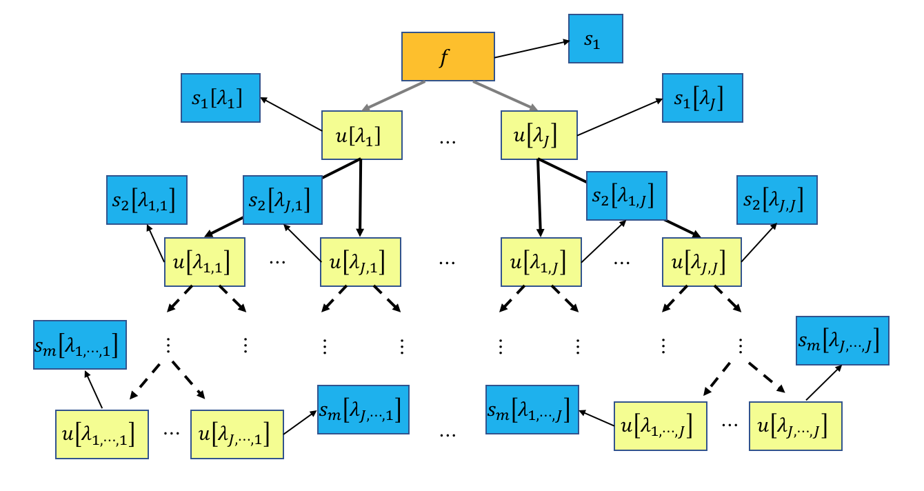
The architecture of the Scattering Transform Network (STN) is a tree-like analog of a convolutional neural network. Figure 1 illustrates its typical architecture.
At the th layer of the STN, we denote , , the index for a multiscale wavelet filter where is the so-called quality factor and is the largest scale of interest at the th layer. Hence, corresponds to the coarsest scale/lowest frequency band whereas corresponds to the finest scale/highest frequency band. By dilating a mother wavelet , we can generate multiscale wavelet filters, i.e.,
| (3) |
where we assume . These correspond to receptive fields of a CNN [3].
Let be an input signal of interest. We define a contraction operator which is Lipschitz continuous, and satisfies the condition . One popular choice of is the modulus operator, i.e., , which we will use in our experiments in Section 3. Let be the set of indices for the th layer. Each internal layer operator is defined by three operations: 1) the (linear) wavelet transform; 2) the contraction operator; 3) subsampling:
| (4) |
where is the subsampling rate. Therefore, there is a path of indices such that
| (5) |
We define the operator for each layer to generate the robust multiscale features of the input signal , which we also call “coefficients” or “representations.”
| (6) |
where represents the averaging function, or father wavelet at a certain scale corresponding to the mother wavelet . After the averaging stage, we can subsample again at rate since the averaging wavelet is a lowpass filter. Note that in particular, for layer , we have .
Note that the GMWs were originally implemented in MATLAB® and disseminated as the JLAB package [10]. We implemented the STN with the option of using either the Morlet wavelets or the GMWs [11] in the Julia programming language [12], and we refer to the STN with the latter option as the GMW-STN. The doublet of parameters of the GMWs in our implementation is set as considering the balance of the time-frequency decays.
3 Music Genre Classification using the GMW-STN
Categorizing recorded music signals into different genres such as classical, country, hiphop, jazz, pop and so on is a difficult task, in part because classification of music genres by human judgment can be subjective and ineffective. In such a classification problem, several CNN-based methods have been proposed, e.g., [13] among others. Although these methods offered some escape routes, they cannot completely escape from the following two fundamental problems (as discussed in Introduction) when they are applied to music signal databases of relatively small size: 1) model overfitting; and 2) interpretability of the intermediate signal representations within CNNs. {hide} The 2D convolutional recurrent neural network (CRNN) was proposed by Choi et al. [choi2017convolutional] for categorizing music. The local deep feature extracted by the convolutional neural network (CNN) and the summarization of the extracted features by the recurrent neural network are shown to achieve effective music classification. Allamy and Koerich [13] also mentioned the effectiveness of 2D CNN [costa2017evaluation] and suggested the use of 1D residual CNN in the GTZAN dataset [14] to automatically classify music genres. Data augmentation may be able to generate enough data and improve the performance [13], but the method heavily depends on the quality of the original dataset and whether the augmentation technique is appropriate. Still, this does not help us understand how to interpret the result from the deep network. It is of interest to know how the features are interpreted so that we can explain the high classification rate with a better understanding of the characteristics of different genres. Hence, such music genre classification with a music signal database of small size is an ideal application to demonstrate the advantage of the STN, in particular, the GMW-STN.
3.1 The GTZAN database and data preparation
In our experiments, we used the so-called GTZAN database [14] contains 1,000 audio/music tracks each of which is 30 second long and was sampled at 22,050Hz. The tracks are evenly distributed into ten music genres: blues; classical; country; disco; hiphop; jazz; metal; pop; reggae; and rock. For each music genre, the 100 tracks were recorded under different conditions.
In our experiments, we split each 30-second track into a set of 15 overlapping segments each of which is 5 second long. Let denote the index of such a music segment. The time interval (indexed by samples) of the th music segment is for , where samples; that is, the hop size is , i.e., the two adjacent segments have second overlap.
In our three-layer STN, we set the subsampling rates and , which generated the following size of the STN coefficients for each input signal of length : the 0th layer: ; the 1st layer: ; the 2nd layer: ; and the 3rd layer: . We also set the quality factors as , and . These numbers mean that we used scales of the form with in the 1st layer, scales of the form with in the 2nd layer, and scales of the form with in the 3rd layer. The first numbers, , , , and , are the size of the output coefficients in each path in the respective layers.
| Layer index | Length |
|---|---|
| Input | 110,250 |
| 1 | (431, 33) |
| 2 | (54, 14, 33) |
| 3 | (7, 10, 14, 33) |
3.2 Interpreting music features in different layers
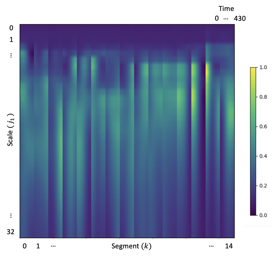
In the 1st layer , we obtained a spectrogram-like STN output as shown in Figure 2(a) for a jazz track. Most of the signal energy resides in low to medium frequency bands.
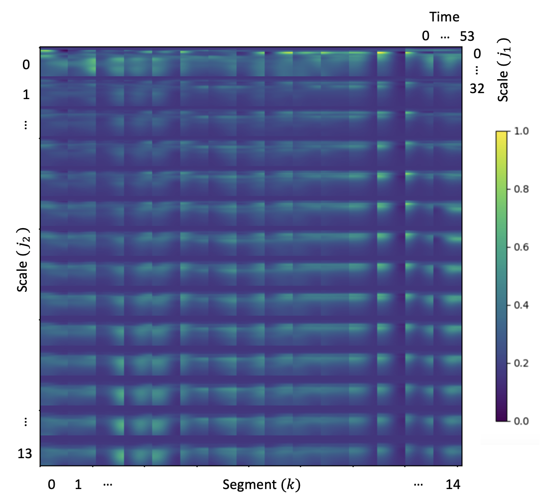
The 2nd layer paths have two different frequency measurements, indexed by where and . Figure 2(b) shows the 2nd layer outputs. Each block in this subfigure represents the 2nd layer outputs corresponding to the 2nd layer scale and the th segment of this jazz track, and the row index within each block corresponds to . The features corresponding to the 2nd layer scale has more variations than those with the larger value of (i.e., finer scales). The larger the value of is, the more stable and less noisy the outputs become. The hierarchical features in the deeper layer of the STN become more invariant (or stable) to the local deformations compared to the 1st layer features. Yet there are many variations across different overlapping segments in the 2nd layer output due to nonstationarity of the jazz music.
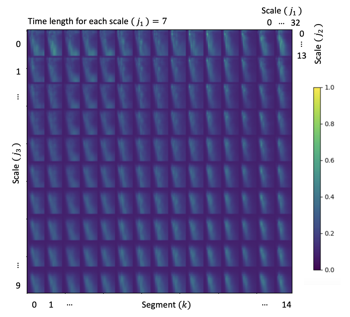
The 3rd layer paths add a third scale variation, indexed by , . Figure 2(c) shows 3rd layer output. Each block in this subfigure represents the 3rd layer outputs indexed by the 3rd layer scale and the th segment of this jazz track, and the row index within each block corresponds to while the columns within each block are organized by and for each , there are coefficients, i.e., the number of columns of each block is . The main advantage of using the 3rd layer is the increased quasi-translation invariance. As in the 2nd layer, we observe more stable patterns when is larger. The major difference from the 2nd layer is that the patterns across different overlapping music segments are more similar in the 3rd layer, which seem to capture intrinsic features of music genre. Thus, the hierarchical features are expected to have more discriminant power to categorize music signals into different music genres.
3.3 Classification experiment settings
We employed the three-fold cross validation scheme and repeated this ten times. In each experiment, the 1,000 music tracks were shuffled and grouped into three folds of 340, 330, and 330 tracks. We used two folds for training and one fold for testing. Then we iterated the process three times by permuting the folds in each of those ten experiments. In other words, we ran the classification experiments 30 times in total. Each fold contains all music genres that are evenly distributed. For instance, there are 34 music files for each music genre in the first fold containing 340 files. In each fold, we further split each music track into 15 segments as described in Section 3.1.
In the training stage, we extracted the STN outputs from all segments in the training set. Then we compressed these outputs using the PCA implemented in the MultivariateStats.jl. We chose the top principal components based on the experimental performance. Then we fed these into a classifier. In the testing stage, we assigned each input file a label based on the majority vote among the labels of its 15 segments predicted by the trained classifier.
In our numerical experiments, we mainly used the Support Vector Machine (SVM) [15, Sec. 3.6] as a classifier of choice. It transforms the input features to new representations in which the different classes are separated with margins that are as wide as possible. The PCA-compressed STN coordinates were fed to the SVM classifier of a polynomial kernel of degree 1 implemented in the LBSVM.jl package [16].Along with the SVM, we also used the GLMNet [15, Chap. 3] in our experiments in order to interpret the classification results in a more intuitive manner. The GLMNet fits a generalized linear model with Lasso regularization through penalized maximum likelihood, and the GLMNet coefficients are denoted by . The regularization path corresponding to the Lasso penalty was computed using cyclic coordinate descent. The significance of the STN coefficients in distinguishing the music genre can be captured by when the mean loss is minimized in the GLMNet.jl package [17].
3.4 Classification results and evaluation
We evaluated performance of various methods by comparing the predicted labels and the ground truth of the music tracks. We computed the classification accuracy by first computing the average accuracy under one experiment of the three-fold cross validation, and then computing the mean of these average accuracies of these ten repeated experiments.
Table 2 shows the superior performance of the GMW-STN with SVM compared to the Morlet-STN with SVM. The novel incorporation of the GMWs into the STN increased the accuracy by more than using the 3rd layer outputs. Moreover, this table indicates that as the number of layers of the STN increases, the classification accuracy also increases regardless of the wavelet filters. The increase in accuracy is most significant from the 1st layer to the 2nd layer.
In comparison to the SVM classifier, the GLMNet classifier performed slightly worse (). However, we will show in Section 4 that the GLMNet classifier can explain the results and shed light on the music information collected from the STN coefficients, which is impossible with the SVM.
| GMW | Morlet | ||
|---|---|---|---|
| Layer | GLMNet | SVM | SVM |
| 1 | 52.3711% | 53.0529% | 48.8776% |
| 2 | 70.2504% | 73.7329% | 70.0517% |
| 3 | 74.5500% | 77.9088% | 73.7178% |
Figure 3 displays the performance of the GMW-STN with SVM for each individual music genre. The GMW-STN with SVM performed best in classifying classical music followed by metal , jazz , and blues . However, it did not perform well in classifying pop and rock . See Section 4 for the explanation on the difference of the accuracies among the music genres.
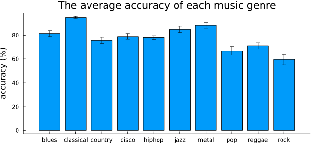
Our result is comparable to the reported accuracy () without data augmentation and () with data augmentation using 1D CNN [13]. However, we can uniquely provide the explanation of the results based on the additional music information retrieved in the layers, by visualizing and interpreting the corresponding STN coefficients. On the other hand, it is quite difficult to explain the results and interpret the intermediate representations in deep learning. Thus, interpretability is a main advantage of our approach over CNNs.
4 Significance of STN Coefficients
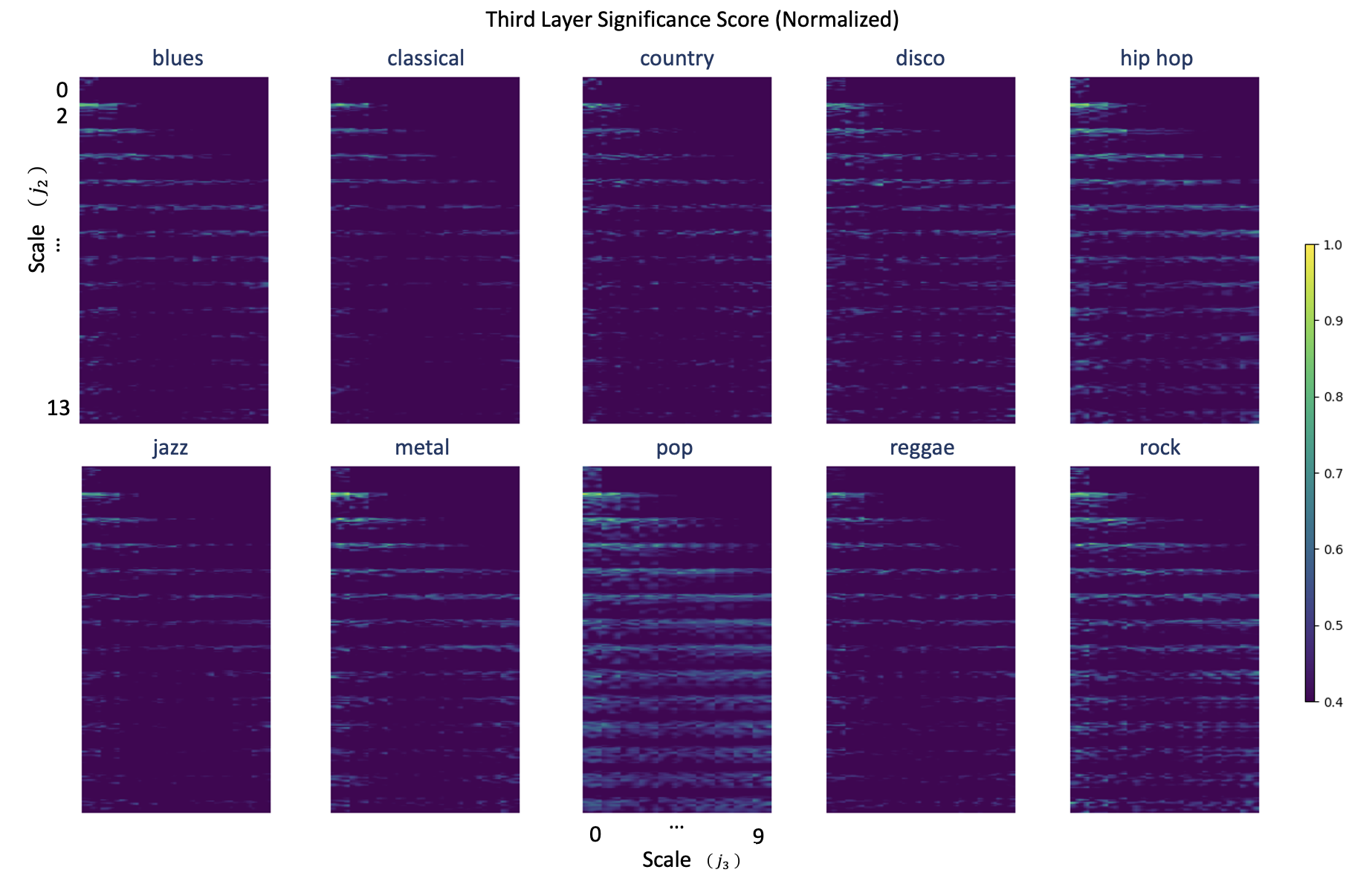
As we mentioned in the previous subsection, the SVM cannot indicate which subset of the STN coefficients mainly contributed to the correct classification results. Unlike the SVM, the GLMNet can provide such information. Since the GLMNet coefficient vector for each genre was computed on the top PCA components of the 3rd layer STN coefficients, we first inverted the PCA to get the corresponding the 3rd layer STN coefficients. Then, we normalized these coefficients so that the maximum value became , which we call the significance scores. Figure 4 displays these significance scores of ten music genres with the lower bound clamped to . It shows that information quantified in the 3rd layer STN is critical in the low frequency portion, especially in the blocks. In general, the concentration in the lower frequency region is positively associated to the high classification rate. For instance, from Figure 4, the classical music has the highest scores in the lower frequency portion of the 3rd layer coefficients while pop and rock have more dispersed score distributions, which can be attributed to the variations of the music patterns in these genres, which in turn may have contributed to the lower classification accuracies for these genres.
5 Conclusions
We demonstrated that the GMW-STN outperformed the conventional STN using the Morlet wavelets. It can be explained by the importance of analyticity of the underlying wavelet transform. In addition, the classification accuracy became higher with more layers in the STN since we could retrieve the more relevant music information that are stable with respect to local deformations in the deeper layer STN coefficients. We could illustrate the connection between the music information retrieved from the GMW-STN and the classification results, which would be impossible using CNNs/DNNs. In addition, it turned out that the lower frequency portion of the music information retrieved from the 3rd layer STN coefficients mainly attributed to the music genre classification performance. In the near future, we plan to explore a 2D STN applied to the spectrograms of the input music tracks.
Acknowledgments
This research was partially supported by the US National Science Foundation grants DMS-1912747, CCF-1934568; the US Office of Naval Research grant N00014-20-1-2381.
References
- [1] Y. LeCun, Y. Bengio, and G. Hinton, “Deep learning,” Nature, vol. 521, no. 7553, pp. 436–444, 2015.
- [2] S. Mallat, “Group invariant scattering,” Comm. Pure Appl. Math., vol. 65, no. 10, pp. 1331–1398, 2012.
- [3] T. Wiatowski and H. Bölcskei, “A mathematical theory of deep convolutional neural networks for feature extraction,” IEEE Trans. Inform. Theory, vol. 64, no. 3, pp. 1845–1866, 2018.
- [4] J. Bruna and S. Mallat, “Classification with scattering operators,” in Proc. IEEE Conf. on Computer Vision and Pattern Recognition (CVPR). IEEE, 2011, pp. 1561–1566.
- [5] ——, “Invariant scattering convolution networks,” IEEE Trans. Pattern Anal. Machine Intell., vol. 35, no. 8, pp. 1872–1886, 2013.
- [6] S. Mallat, A Wavelet Tour of Signal Processing, 3rd ed. Burlington, MA: Academic Press, 2009.
- [7] J. M. Lilly and S. C. Olhede, “On the analytic wavelet transform,” IEEE Trans. Inform. Theory, vol. 56, no. 8, pp. 4135–4156, 2010.
- [8] S. C. Olhede and A. T. Walden, “Generalized morse wavelets,” IEEE Trans. Signal Process., vol. 50, no. 11, pp. 2661–2670, 2002.
- [9] J. M. Lilly and S. C. Olhede, “Generalized Morse wavelets as a superfamily of analytic wavelets,” IEEE Trans. Signal Process., vol. 60, no. 11, pp. 6036–6041, 2012.
- [10] ——, “Higher-order properties of analytic wavelets,” IEEE Trans. Signal Process., vol. 57, no. 1, pp. 146–160, 2009.
- [11] D. Weber, “Scatteringtransform.jl: An implementation of the generalized scattering transform,” https://github.com/dsweber2/ScatteringTransform.jl, 2021.
- [12] J. Bezanson, A. Edelman, S. Karpinski, and V. B. Shah, “Julia: A fresh approach to numerical computing,” SIAM Review, vol. 59, no. 1, pp. 65–98, 2017. [Online]. Available: https://doi.org/10.1137/141000671
- [13] S. Allamy and A. L. Koerich, “1D CNN architectures for music genre classification,” in 2021 IEEE Symposium Series on Computational Intelligence (SSCI). IEEE, 2021, pp. 01–07.
- [14] G. Tzanetakis and P. Cook, “Musical genre classification of audio signals,” IEEE Trans. Speech Audio Process., vol. 10, no. 5, pp. 293–302, 2002.
- [15] T. Hastie, R. Tibshirani, and M. Wainwright, Statistical Learning with Sparsity: The Lasso and Generalizations, ser. Monographs on Statistics and Applied Probability. Boca Raton, FL: CRC Press, 2015, vol. 143.
- [16] S. Kornblith and M. Pastell, “LIBSVM.jl: A Julia interface for libsvm,” https://github.com/JuliaML/LIBSVM.jl, 2021.
- [17] J. Statistics, “GLMNet.jl: Julia wrapper for fitting Lasso/ElasticNet GLM models using glmnet,” https://github.com/JuliaStats/GLMNet.jl, 2021.