Efficient Approximation of
Expected Hypervolume Improvement
using Gauss-Hermite Quadrature

Abstract

Many methods for performing multi-objective optimisation of computationally expensive problems have been proposed recently. Typically, a probabilistic surrogate for each objective is constructed from an initial dataset. The surrogates can then be used to produce predictive densities in the objective space for any solution. Using the predictive densities, we can compute the expected hypervolume improvement (EHVI) due to a solution. Maximising the EHVI, we can locate the most promising solution that may be expensively evaluated next. There are closed-form expressions for computing the EHVI, integrating over the multivariate predictive densities. However, they require partitioning the objective space, which can be prohibitively expensive for more than three objectives. Furthermore, there are no closed-form expressions for a problem where the predictive densities are dependent, capturing the correlations between objectives. Monte Carlo approximation is used instead in such cases, which is not cheap. Hence, the need to develop new accurate but cheaper approximation methods remains. Here we investigate an alternative approach toward approximating the EHVI using Gauss-Hermite quadrature. We show that it can be an accurate alternative to Monte Carlo for both independent and correlated predictive densities with statistically significant rank correlations for a range of popular test problems.

1 Introduction

Many real-world optimisation problems have multiple conflicting objectives [9, 21, 26]. In many cases, these objective functions can take a substantial amount of time for one evaluation. For instance, problems involving computational fluid dynamic simulations can take minutes to days for evaluating a single design (or decision vector/candidate solution) [2, 6]. Such problems do not have analytical or closed-form expressions for the objective functions and are termed as black-box problems. To alleviate the computation time and obtain solutions with few expensive function evaluations, surrogate-assisted optimisation methods [3, 5], e.g. Bayesian optimisation (BO) [25], have been widely used. In such methods, a surrogate model (also known as a metamodel) is built on given data (which is either available or can be generated with some design of experiment technique [22]). If one builds independent models for each objective function [14, 29], the correlation between the objective functions is not directly considered. Multi-task surrogates [4, 24] have been used recently to consider the correlation.

In BO, the surrogate model is usually a Gaussian process (GP) because GPs provide uncertainty information in the approximation in addition to the point approximation. These models are then used in optimising an acquisition function (or infill criterion) to find the next best decision vector to evaluate expensively. The acquisition function usually balances the convergence and diversity. Many acquisition functions have been proposed in the literature. Here, we focus on using expected hypervolume improvement (EHVI) [12], which has become a popular and well-studied acquisition function for expensive multi-objective optimisation largely due to its reliance on the hypervolume [30] (the only strictly Pareto compliant indicator known so far). The EHVI relies on a predictive distribution of solutions (with either independent [12] or correlated objective functions [24]). An optimiser is used to maximise the EHVI to find a decision vector with maximum expected improvement in hypervolume. The EHVI can be computed analytically for any number of objectives assuming the objective functions $f_{1},\dots,f_{m}$ are drawn from independent GPs [14]. However, this computation is expensive for more than three objectives. Monte Carlo (MC) approximation of EHVI is often used instead in such cases but this is not cheap. Consequently, there is a need for accurate but cheaper approximation methods for EHVI. We propose and investigate a novel way of approximating the EHVI using Gauss-Hermite (GH) quadrature [18, 20]. In essence, GH approximates the integral of a function using a weighted sum resulting in fewer samples to approximate the EHVI.

The rest of the article is structured as follows. In Section 2, we briefly describe multivariate predictive densities and EHVI, and then introduce the GH method in Section 3. In Section 4, we show the potential of the proposed idea of using GH by comparing it with analytical and MC approximations (for 2-3 objectives). Finally, conclusions are drawn in Section 5.

2 Background

For multi-objective optimisation problems with $m$ objective functions to be minimised, given two vectors $\mathbf{z}$ and $\mathbf{y}$ in the objective space, we say that $\mathbf{z}$ dominates $\mathbf{y}$ if $z_{i}\leq y_{i}$ for all $i=1,\dots,m$ and $z_{j}<y_{j}$ for at least one index $j$. A solution is Pareto optimal if no feasible solution dominates it. The set of Pareto optimal solutions in the objective space is called a Pareto front.

In multi-objective BO, the predictive distribution due to a solution with independent models is defined as:

$$\mathbf{y}\sim\mathcal{N}(\bm{\mu},\operatorname*{diag}(\sigma^{2}_{1},\dots,\sigma^{2}_{m})),$$

where $m$ is the number of objectives and $\bm{\mu}=(\mu_{1},\dots,\mu_{m})^{\top}$ is the mean vector, with $\mu_{i}$ and $\sigma_{i}$ being the mean and standard deviations of the predictive density for the $i^{th}$ objective. To quantify the correlation between objectives, a multi-task surrogate model can be used. The distribution of a solution with a single multi-task model is defined with a multi-variate Gaussian distribution:

$$\mathbf{y}\sim\mathcal{N}(\bm{\mu},\Sigma),$$

where $\bm{\mu}$ is the vector of means and $\Sigma$ is the covariance matrix that quantifies the correlation between different objectives. It should be noted that considering only the diagonal elements of $\Sigma$ would ignore any correlations between objectives, and result in an independent multivariate predictive density.

The hypervolume measure [30] is a popular indicator to assess the quality of a set of solutions to a multi-objective optimisation problem. Thus it is often used to compare multi-objective optimisation algorithms or for driving the search of indicator-based multi-objective optimisation algorithms. The EHVI answers the question of what the expected improvement of the hypervolume is if some new candidate solution $\mathbf{x}$ would be added to an existing set of solutions. Consequently, the solution with the highest EHVI may be the one worth an expensive function evaluation. To avoid ambiguity, in the following, we provide formal definitions of the concepts discussed here, before discussing methods to calculate the EHVI.

Definition 1 (Hypervolume indicator)

Given a finite set of $k$ points (candidate solutions) $P=\{\mathbf{p}_{1},\dots,\mathbf{p}_{k}\}\subset\mathbf{R}^{m}$ where $\mathbf{p}_{i}=(f_{1}(\mathbf{x}_{i}),\dots,f_{m}(\mathbf{x}_{i})))^{\top}$ for an optimisation problem with $m$ objectives, the hypervolume indicator (HI) of $P$ is defined as the Lebesgue measure of the subspace (in the objective space) dominated by $P$ and a user-defined reference point $\mathbf{r}$ [29]:

$$HI(P)=\Lambda(\cup_{\mathbf{p}\in P}[\mathbf{p},\mathbf{r}]),$$

where $\Lambda$ is the Lebesgue measure on $\mathbf{R}^{m}$, and $\mathbf{r}$ chosen such that it is dominated by all points in $P$, and ideally also by all points of the Pareto front.

Definition 2 (Hypervolume contribution)

Given a point $\mathbf{p}\in P$, its hypervolume contribution with respect to $P$ is $\Delta HI(P,\mathbf{p})=HI(P)-HI(P\backslash\{\mathbf{p}\})$.

Definition 3 (Hypervolume improvement)

Given a point $\mathbf{p}\notin P$, its hypervolume improvement with respect to $P$ is $I(\mathbf{p},P)=HI(P\cup\{\mathbf{p}\})-HI(P)$.

Definition 4 (Expected hypervolume improvement)

Given a point $\mathbf{p}\notin P$, its expected hypervolume improvement (EHVI) with respect to $P$ is

$$\int_{\mathbf{p}\in\mathbb{R}^{m}}HI(P,\mathbf{p})\cdot PDF(\mathbf{p})d\mathbf{p},$$

where $PDF(\mathbf{p})$ is the predictive distribution function of $\mathbf{p}$ over points in the objective space.

The EHVI can be computed analytically for any number of objectives assuming they are uncorrelated, but this requires partitioning the objective space, which can be prohibitively expensive for $m>3$ objectives. Consequently, there is considerable interest in finding more efficient ways to compute EHVI, see e.g. [7, 8, 13, 14, 17, 28]. MC integration is an alternative to an exact computation of EHVI. It is easy to use in practice and has been the method of choice for problems with $m>3$ objectives. Given a multivariate Gaussian distribution from which samples are drawn, or $\mathbf{p}_{i}\sim\mathcal{N}(\bm{\mu},\Sigma)$, and a set of points $P$ (e.g. an approximation of the Pareto front), then the MC approximation of EHVI across $c$ samples is

$$\frac{1}{c}\sum_{i=1}^{c}I(\mathbf{p}_{i},P),$$ (1)

where $I(\mathbf{p}_{i},P)$ is the hypervolume improvement (see Definition 3). The approximation error is given by $e=\sigma_{\text{M}}/\sqrt{c}$, where $\sigma_{\text{M}}$ is the sample standard deviation [19]. Clearly, as the sample size $c$ increases, the approximation error reduces, namely in proportion to $1/\sqrt{c}$. In other words, a hundred times more samples will result in improving the accuracy by ten times.

Typically, evaluating the improvement due to a single sample can be rapid. Even if we consider a large $c$, it is often not that time-consuming to compute the EHVI for a single predictive density. However, when we are optimising EHVI to locate the distribution that is the most promising in improving the current approximation of the front, an MC approach may become prohibitively expensive with a large enough $c$ for an acceptable error level. Therefore, alternative approximation methods that are less computationally intensive are of interest. In the next section, we discuss such an approach based on GH quadrature.

3 Gauss-Hermite approximation

The idea of GH approximation is based on the concept of Gaussian quadratures, which implies that if a function $f$ can be approximated well by a polynomial of order $2n-1$ or less, then a quadrature with $n$ nodes suffices for a good approximation of a (potentially intractable) integral [18, 20], i.e.

$$\int_{D}f(\mathbf{x})\psi(\mathbf{x})\,dx\;\approx\;\sum_{i=1}^{n}w_{i}f(\mathbf{x}_{i}),$$

where $D$ is the domain over which $f(\mathbf{x})$ is defined, and $\psi$ a known weighting kernel (or probability density function). The domain $D$ and weighing kernel $\psi$ define a set of $n$ weighted nodes $\mathcal{S}=\{\mathbf{x}_{i},w_{i}\},i=1,\dots,n$, where $\mathbf{x}_{i}$ is the $i$th deterministically chosen node and $w_{i}$ its associated quadrature weight. We refer to this concept as Gauss-Hermite if $D$ is infinite, i.e., $D\in(-\infty,\infty)$, and the weighting kernel $\psi$ is given by the density of a standard Gaussian distribution.

The location of the nodes $\mathbf{x}_{i}$ are determined using the roots of the polynomial of order $n$, while the weights $w_{i}$ are computed from a linear system upon computing the roots [18]; the interested reader is referred to [23] for technical details of this calculation. Intuitively, one can think of the selected nodes as representatives of the Gaussian distribution with the weights ensuring convergence as $n$ increases and a low approximation error for a given $n$ [11].

Extending the one-dimensional GH quadrature calculations to multivariate integrals is achieved by expanding the one-dimensional grid of nodes to form an $m$-dimensional grid, which is then pruned, rotated, scaled, and, finally, the nodes are translated. Figure 1 illustrates the key steps of this process for a two-dimensional ($m=2$) integral. The weights of the $m$-variate quadrature points are the product of the corresponding $m$ one-dimensional weights; for $m=2$, this leads to the following two-dimensional Gaussian quadrature approximation:

$$\sum_{i=1,j=1}^{n,n}w_{i}w_{j}f(\mathbf{x}_{i},\mathbf{x}_{j}).$$

The pruning step eliminates nodes that are associated with a low weight (i.e., points on the diagonal as they are further away from the origin); such nodes do not contribute significantly to the total integral value, hence eliminating them improves computational efficiency. Rotating, scaling and translating nodes account for correlations across dimensions, which is often present in practice. The rotation and scaling are conducted using a rotation matrix constructed from the dot product of the eigenvector and the eigenvalues of the covariance matrix, and the translation is performed by adding the mean vector.

(a) Sampling

(b) Pruning

(c) Rotation

Figure 1: An illustration of the process of generating the nodes and the associated weights using the GH quadrature for a two-dimensional ($m=2$) Gaussian density with the mean vector $\bm{\mu}=(0,0)^{\top}$ and the covariance matrix $\Sigma=\begin{pmatrix}1&0.5\\ 0.5&1\end{pmatrix}$. The parameters used are: $n=8$ points per dimension and a pruning rate of $r=0.2$ (i.e., 20%). The dots represent the nodes, and the colours represent the respective weights. The contours show the Gaussian density with the outermost contour corresponding to two-standard deviation.

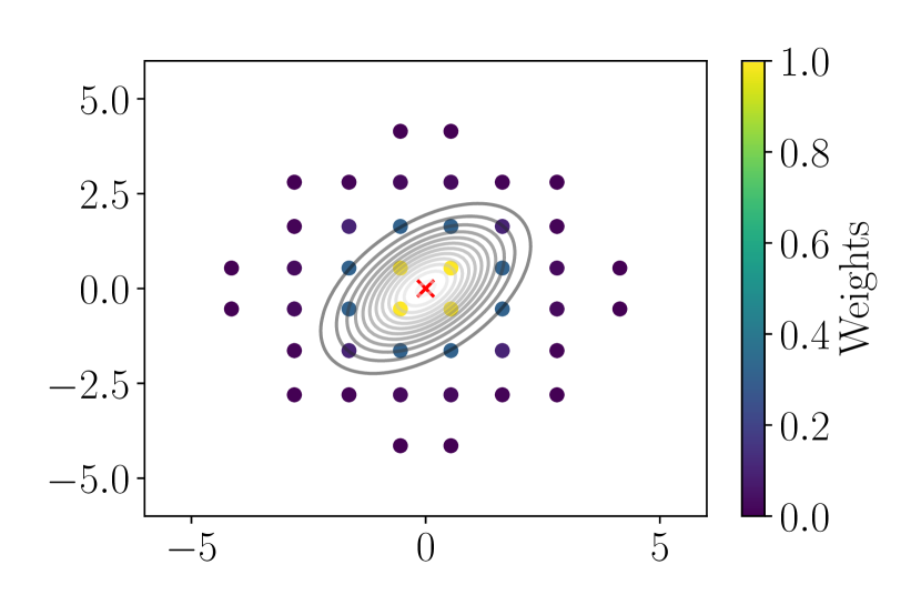
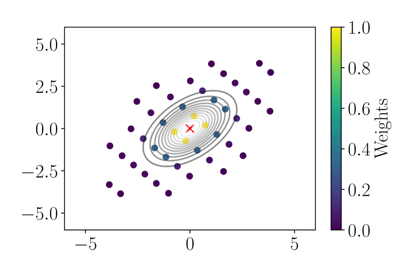
Note that this approach may result in a combinatorial explosion of nodes in approximating a high-dimensional multivariate Gaussian distribution. Given $n$ nodes per dimension for an $m$-dimensional space, the total number of nodes generated is $K=\lfloor n^{m}(1-r)\rfloor$, where $r\in[0,1]$ is the pruning rate (the greater $r$, the more nodes are discarded with $r=0$ corresponding to not discarding any nodes). For instance, using $n=5$, $m=10$ and $r=0.2$, we have $K=7812500$ nodes. Clearly, this would be computationally more expensive than MC approximation. Therefore, for high-dimensional integration the default GH approach may not be suitable. As a rule of thumb, we propose that if the number of nodes from GH goes beyond the number of samples required for a good MC approximation, then one should use the latter, instead.

It should be noted that there is some work on high-dimensional GH approximations, e.g. [15], but we do not investigate these in this paper.

3.1 Gauss-Hermite for approximating EHVI

To approximate the EHVI, we use $K$ samples (nodes) and associated weights from GH quadrature as follows:

$$\sum_{i=1}^{K}\omega_{i}I(\mathbf{p}_{i},P),$$ (2)

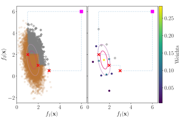
where $P$ is the approximated Pareto front, $\mathbf{p}_{i}$ is the $i$th sample, and $\omega_{i}=\prod_{j=1}^{m}w_{j}(\mathbf{x}_{i})$ is the weight in an $m$-dimensional objective space corresponding to the sample $\mathbf{x}_{i}$. This is effectively a weighted sum of the contributions, where the weights vary according to the probability density. This is also illustrated in the right panel of Figure 2: The dots show the GH samples (nodes). The grid of points covers an area that is consistent with the underlying Gaussian distribution. Since we know how the probability density varies, we can generate proportional weights, which in turn permits us to derive a good approximation with only a few points in the grid.

On the other hand, with MC in (1), every sample (dots in Figure 2, left panel) contributes equally to the average EHVI. Hence, a sample is somewhat unrelated to the intensity of the underlying probability density at that location. As such, with few samples, we may not derive a good approximation. It should be noted that the gray diamonds (in both panels) are dominated by the approximation of the Pareto front, and therefore there is no improvement (see Definition 3) due to these solutions. Hence, these gray diamonds do not contribute to the EHVI for either of the methods.

Figure 2: A visual comparison of MC (left) and GH (right) samples in the objective space (assuming a minimisation problem). The approximation of the Pareto front is depicted with red crosses, and the reference vector $\mathbf{r}$ for hypervolume computation is shown with a magenta square. The blue dashed line outlines the dominated area. We used a two-variate Gaussian distribution to generate samples with the mean vector $\bm{\mu}=(1.5,1.5)^{\top}$ and the covariance matrix $\Sigma=\begin{pmatrix}0.16&-0.15\\ -0.15&1.01\end{pmatrix}$; the pick contours represent this density. The gray diamonds are dominated by the approximated front.

4 Experimental study

In this section, we focus on comparing the accuracy of GH and MC approximations with respect to the analytical calculation of EHVI ($A$) introduced in [7, 14]. As the analytical method is only suitable for independent multivariate Gaussian densities, we firstly investigate the efficacy of the approximation methods for uncorrelated densities for $m=2$ and $3$, and then expand our exploration to correlated multivariate densities. We use popular test problems: DTLZ 1-4, 7 [10], and WFG 1-9 [16]. They were chosen as they allow us to validate the efficacy of the approximation methods for Pareto fronts with diverse features; e.g., DTLZ2 and WFG4 have concave, DTLZ7 and WFG2 have disconnected, and DTLZ1 and WFG3 have linear Pareto fronts.

Our strategy was to first generate a random multivariate distribution, and then, for an approximation of the known Pareto front, compute the EHVI due to this random distribution analytically and with the two approximation methods (GH and MC). Using this approach, we aimed to collect data on a range of randomly generated multivariate distributions and inspect the agreement between analytical measurements and approximations. To quantify this, we used Kendall’s $\tau$ rank correlation test [1], which varies between $[-1,1]$ with $1$ showing perfectly (positively) correlated ordering of the data by a pair of competing methods. The test also permits the estimation of a $p$-value, which, if below a predefined level $\alpha$ indicates that results are significant. In this paper, we set $\alpha=0.05$, however, in all cases, we found the $p$-value to be practically zero, hence indicating significance in the results.

To implement the GH approximation, we converted existing R code into Python; our code is available to download at github.com/AlmaRahat/EHVI_Gauss-Hermite. If not stated otherwise, MC uses $10,000$ samples, and GH uses a pruning rate of $r=0.2$. For GH, we investigate different numbers of nodes (points) $n$ per dimension, and use the notation $GH_{n}$ to indicate this number. Any results reported are results obtained across $100$ randomly generated multivariate Gaussian distributions to generate as many EHVIs.

4.1 Uncorrelated multivariate Gaussian distribution

To generate a random multivariate distribution, we first take a reference front $P$. We then calculate the maximum $p_{\max}^{i}$ and minimum $p_{\min}^{i}$ values along each objective function $f_{i}$. The span along the $i$th objective is thus $s=p_{\max}^{i}-p_{\min}^{i}$. Using this, we construct a hyper-rectangle $H$ which has lower and upper bounds at vectors $\mathbf{l}=(l_{1},\dots,l_{m})$ and $\mathbf{u}=(u_{1},\dots,u_{m})$, respectively, with $l_{i}=p_{\min}^{i}-0.3s$ and $u_{i}=p_{\max}^{i}+0.3s$. We take a sample from $H$ uniformly at random to generate a mean vector $\bm{\mu}$. The covariance matrix must be a diagonal matrix with positive elements for an independent multivariate distribution. Hence, we generate the $i$th diagonal element by sampling uniformly at random in the range $[0,u_{i}-l_{i}]$.

(a)

(b)

(c)

Figure 3: Efficacy of MC and GH (with $15$ points per dimension, $GH_{15}$) approximations in comparison to analytical measurements of EHVI for the DTLZ2 problem with $2$ objectives and $100$ randomly generated multivariate Gaussian distributions. The dotted red-line depicts the performance of the perfect approximations. MC approximations used $10,000$ samples. In all cases, we observe strong rank correlations with Kendall’s $\tau$ coefficient over $0.97$ with practically zero $p$-values.

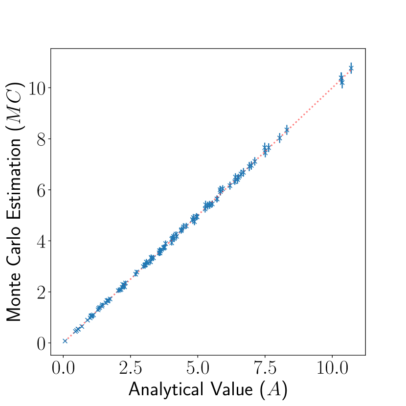
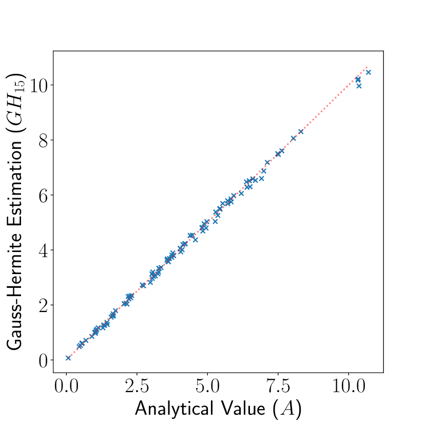
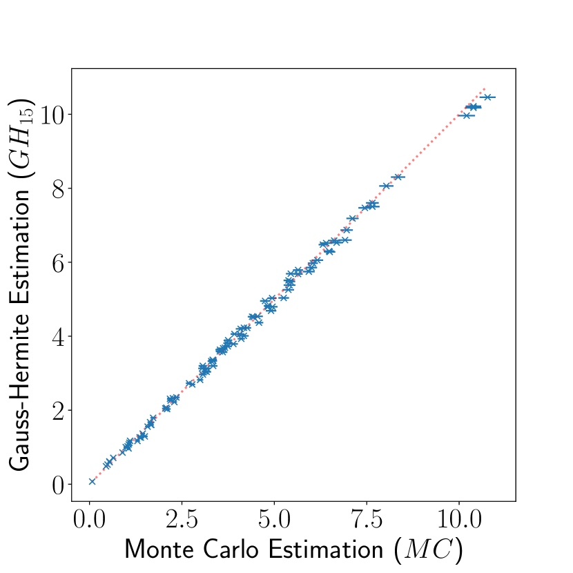
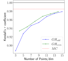
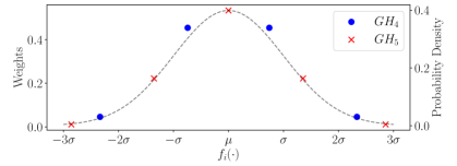
Figure 3 shows an example comparison between the analytical (A), MC and GH computations of EHVI for DTLZ2. The comparisons clearly show that the performances of MC and $GH_{15}$ are reliable with respect to $A$ with a Kendall’s $\tau$ coefficient of over $0.97$ and associated $p$-value of (almost) zero. To investigate if there is an increase in accuracy with the number of points per dimension, we repeated the experiment by varying the number of points per dimension between $3$ and $15$ (see Figure 4 for results on the DTLZ2 problem with $m=2$). Interestingly, there is a difference between having an odd or an even number of points per dimension: there is often a dip in performance when we go from even to odd. In Figure 4, we see that there is a slight decrease in the rank coefficient between $4$ and $5$ points per dimension. We attribute this decrease to how the points are distributed for odd and even numbers of points per dimension. When we have an odd number of points for GH, it produces a node at the mean of the distribution. If there is an even number of points per dimensions, there is no node at the mean (see Figure 5). Because of this, the approximation may vary between odd and even number of points. Nonetheless, the monotonicity in accuracy improvement is preserved when the number of points is increased by two.

Figure 4: Increase in accuracy with the increase in the number of points per dimension between $3$ to $15$ for the GH approximation with respect to the analytical result for DTLZ2 ($m=2$) and $100$ random multivariate distributions. The black horizontal line shows the theoretical upper bound for Kendall’s $\tau$ coefficient. The red dashed horizontal line shows the coefficient for the EHVI using MC. The blue and red lines depict the increase in coefficient as we increase the number of points per dimensions for odd and even numbers, respectively, for GH.

Figure 5: An example of the distribution of GH nodes for $4$ ($GH_{4}$) and $5$ ($GH_{5}$) points per dimension (before pruning) for the standard Gaussian density with the mean $\mu=0$ and the standard deviation $\sigma=1$ (shown in dashed black line).

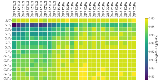
We took the same approach to investigate the efficacy of GH and MC in all the test problems for $m=2$ and $3$. The results of the comparison are summarised in Figure 6. We observed the same trends that with the increase in the number of points per dimension, we increase the accuracy. Even with a small number of points per dimension we are able to derive coefficients of over $0.85$ for all the problems. Interestingly, in some instances, e.g., WFG3 ($m=3$) and WFG4 ($m=2$), we clearly get better approximations from GH in comparison to MC.

Figure 6: Performance comparison of MC and GH ($GH_{n}$, where $n$ is the number of points per dimension) with respect to the analytical EHVI for a range of test problems with $100$ randomly generated multivariate Gaussian distributions in each instance. Lighter colours correspond to better coefficient values.

4.2 Correlated multivariate Gaussian distribution

The key issue with the analytical formula for EHVI is that it does not cater for correlated multivariate predictive distributions. However, both MC and GH, even though they are computationally relatively intensive, do not suffer from this issue. To investigate the efficacy of different methods, again, we take the same approach as before. We generate random distributions and compute the EHVI values with A, MC and GH, and then evaluate the rank correlations using Kendall’s $\tau$ coefficient. Importantly, the most reliable method in this case is MC.

In this instance, the process to generate a random mean vector remains the same. However, for a valid covariance matrix, we must ensure that the randomly generated matrix remains positive definite. We, therefore, use Wishart distribution [27] to generate a positive definite matrix that is scaled by $\operatorname*{diag}(u_{1}-l_{1},\dots,u_{m}-l_{m})$. To demonstrate that the analytical version for uncorrelated distributions generates a poor approximation for the EHVI due to a correlated distribution, we use the diagonal of the covariance matrix and ignore the off-diagonal elements, and compute the EHVI. This allows us to quantitatively show that GH may be a better alternative to MC from an accuracy perspective.

(a)

(b)

(c)

(d)

Figure 7: Illustration of the efficacy of GH for correlated multivariate Gaussian distributions as Figure 3 in 7(a) – 7(c) for DTLZ2 ($m=2$). In 7(d), we show the summary of efficacies for different approximation methods when compared to MC across all DTLZ and WFG problems (for $m=2$ and $m=3$). Analytical approximations were generated using the diagonal of the covariance matrix.

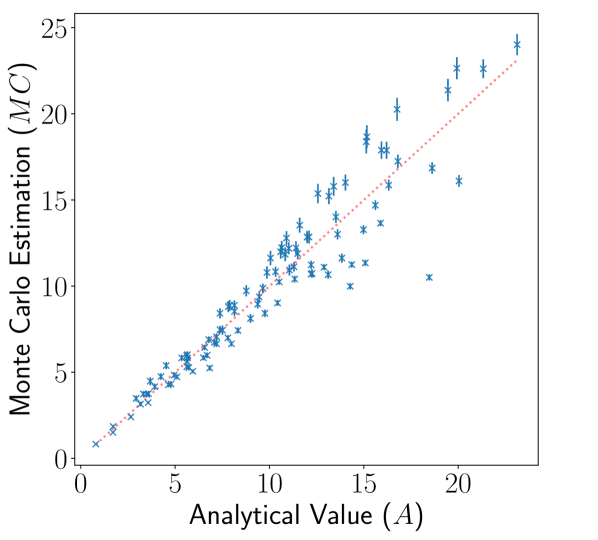
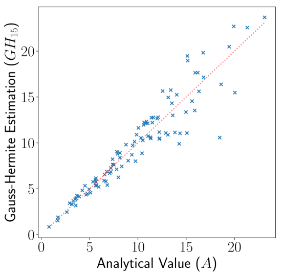
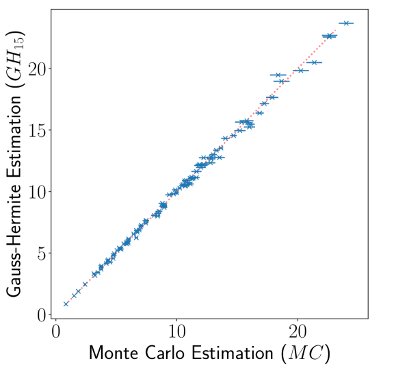
In Figures 7(a) – 7(c), we show the comparison between different methods for computing EHVI for the DTLZ2 problem with $m=2$. Here, $A$ somewhat agrees with MC and $GH_{15}$ with a correlation coefficient of approximately $0.84$ in each case. However, MC and $GH_{15}$ are essentially producing the same ranking of solutions with a coefficient of just over $0.97$. Therefore, $GH_{15}$ with $180$ nodes is an excellent alternative to MC with $10,000$ samples. The results on DTLZ2 do not appear too bad for $A$. To ensure that this is the case for all test problems under scrutiny, we repeated the experiments, but this time generating $100$ random multivariate correlated Gaussian distributions in each instance. Here, we assumed that MC is the most reliable measure, and computed the Kendall’s $\tau$ coefficient with respect to MC. The correlation coefficient distributions for A and $GH_{n}$s are given in Figure 7(d). Clearly, there is a wide variance in the performance of A, with the minimum being $0.39$ for WFG7 ($m=3$) and maximum being $0.9$ for DTLZ1 ($m=2$). On the other hand, $GH_{3}$ produced the worst performance for GH across the board, but that was at $0.86$ for DTLZ ($m=2$), which shows a strong rank correlation. This shows that just considering the diagonal of the covariance matrix and computing the analytical EHVI is not a reliable approximation method under a correlated multivariate predictive density. Instead, GH can produce a solid approximation with very few points.

5 Conclusions

EHVI is a popular acquisition function for expensive multi-objective optimisation. Computing it analytically is possible for independent objectives (predictive densities). However, this can be prohibitively expensive for more than 3 objectives. Monte Carlo approximation can be used instead, but this is not cheap. We proposed an approach using GH quadrature as an alternative to approximating EHVI. Our experimental study showed that GH can be an accurate alternative to MC for both independent and correlated predictive densities with statistically significant rank correlations for a range of popular test problems. Future work can look at improving the computational efficiency of GH for high-dimensional problems, and validating GH within BO using EHVI as the acquisition function.

References

- [1] Abdi, H.: The Kendall rank correlation coefficient. In: Salkind, N.J. (ed.) Encyclopedia of Measurement and Statistics, pp. 508–510. Sage Publications, Thousand Oaks, CA (2007)
- [2] Allmendinger, R.: Tuning evolutionary search for closed-loop optimization. Ph.D. thesis, The University of Manchester (2012)
- [3] Allmendinger, R., Emmerich, M.T., Hakanen, J., Jin, Y., Rigoni, E.: Surrogate-assisted multicriteria optimization: Complexities, prospective solutions, and business case. Journal of Multi-Criteria Decision Analysis 24(1-2), 5–24 (2017)
- [4] Bonilla, E.V., Chai, K., Williams, C.: Multi-task Gaussian process prediction. In: Proceedings of the 20th International Conference on Neural Information Processing Systems. pp. 153–160 (2007)
- [5] Chugh, T., Sindhya, K., Hakanen, J., Miettinen, K.: A survey on handling computationally expensive multiobjective optimization problems with evolutionary algorithms. Soft Computing 23(9), 3137–3166 (2019)
- [6] Chugh, T., Sindhya, K., Miettinen, K., Jin, Y., Kratky, T., Makkonen, P.: Surrogate-assisted evolutionary multiobjective shape optimization of an air intake ventilation system. In: Proceedings of the 2017 IEEE Congress on Evolutionary Computation (CEC). pp. 1541–1548. IEEE (2017)
- [7] Couckuyt, I., Deschrijver, D., Dhaene, T.: Fast calculation of multiobjective probability of improvement and expected improvement criteria for pareto optimization. Journal of Global Optimization 60(3), 575–594 (2014)
- [8] Daulton, S., Balandat, M., Bakshy, E.: Differentiable expected hypervolume improvement for parallel multi-objective Bayesian optimization. Advances in Neural Information Processing Systems 33, 9851–9864 (2020)
- [9] Deb, K.: Multi-objective optimization. In: Burke, E.K., Kendall, G. (eds.) Search Methodologies, pp. 403–449. Springer (2014)
- [10] Deb, K., Thiele, L., Laumanns, M., Zitzler, E.: Scalable test problems for evolutionary multiobjective optimization. In: Evolutionary multiobjective optimization, pp. 105–145. Springer (2005)
- [11] Elvira, V., Closas, P., Martino, L.: Gauss-Hermite quadrature for non-Gaussian inference via an importance sampling interpretation. In: Proceedings of the 2019 27th European Signal Processing Conference (EUSIPCO). pp. 1–5. IEEE (2019)
- [12] Emmerich, M.: Single- and multi-objective evolutionary design optimization assisted by Gaussian random field metamodels. Ph.D. thesis, TU Dortmund (2005)
- [13] Emmerich, M., Yang, K., Deutz, A., Wang, H., Fonseca, C.M.: A multicriteria generalization of Bayesian global optimization. In: Advances in Stochastic and Deterministic Global Optimization, pp. 229–242. Springer (2016)
- [14] Emmerich, M.T., Deutz, A.H., Klinkenberg, J.W.: Hypervolume-based expected improvement: Monotonicity properties and exact computation. In: 2011 IEEE Congress of Evolutionary Computation (CEC). pp. 2147–2154. IEEE (2011)
- [15] Holtz, M.: Sparse grid quadrature in high dimensions with applications in finance and insurance. Ph.D. thesis, Institut für Numerische Simulation, Universität Bonn (2008)
- [16] Huband, S., Hingston, P., Barone, L., While, L.: A review of multiobjective test problems and a scalable test problem toolkit. IEEE Transactions on Evolutionary Computation 10(5), 477–506 (2006)
- [17] Hupkens, I., Deutz, A., Yang, K., Emmerich, M.: Faster exact algorithms for computing expected hypervolume improvement. In: Gaspar-Cunha, A., Antunes, C.H., Coello Coello, C. (eds.) Evolutionary Multi-criterion Optimization, 8th International Conference, Proceedings. pp. 65–79. Springer (2015)
- [18] Jäckel, P.: A note on multivariate Gauss-Hermite quadrature. London: ABN-Amro. Re (2005)
- [19] Koehler, E., Brown, E., Haneuse, S.J.P.: On the assessment of Monte Carlo error in simulation-based statistical analyses. The American Statistician 63(2), 155–162 (2009)
- [20] Liu, Q., Pierce, D.A.: A note on Gauss-Hermite quadrature. Biometrika 81(3), 624–629 (1994)
- [21] Miettinen, K.: Nonlinear Multiobjective Optimization. Kluwer Academic Publishers (1999)
- [22] Montgomery, D.C.: Design and Analysis of Experiments. John Wiley & Sons (2017)
- [23] Press, W.H., Teukolsky, S.A., Vetterling, W.T., Flannery, B.P.: Numerical Recipes in C. Oxford University Press (1992)
- [24] Shah, A., Ghahramani, Z.: Pareto frontier learning with expensive correlated objectives. In: Proceedings of the 33rd International Conference on Machine Learning. pp. 1919–1927 (2016)
- [25] Shahriari, B., Swersky, K., Wang, Z., Adams, R.P., de Freitas, N.: Taking the human out of the loop: A review of Bayesian optimization. Proceedings of the IEEE 104(1), 148–175 (2016)
- [26] Stewart, T., Bandte, O., Braun, H., Chakraborti, N., Ehrgott, M., Göbelt, M., Jin, Y., Nakayama, H., Poles, S., Di Stefano, D.: Real-world applications of multiobjective optimization. In: Branke, J., Deb, K., Miettinen, K., Slowinski, R. (eds.) Multiobjective Optimization: Interactive and Evolutionary Approaches, pp. 285–327. Springer, Berlin, Heidelberg (2008)
- [27] Wishart, J.: The generalised product moment distribution in samples from a normal multivariate population. Biometrika 20A(1–2), 32–52 (1928)
- [28] Yang, K., Emmerich, M., Deutz, A., Fonseca, C.M.: Computing 3-D expected hypervolume improvement and related integrals in asymptotically optimal time. In: Trautmann, H., Rudolph, G., Klamroth, K. andr Schütze, O., Wiecek, M., Jin, Y., Grimme, C. (eds.) Evolutionary Multi-Criterion Optimization, 9th International Conference, Proceedings. pp. 685–700. Springer (2017)
- [29] Yang, K., Gaida, D., Bäck, T., Emmerich, M.: Expected hypervolume improvement algorithm for PID controller tuning and the multiobjective dynamical control of a biogas plant. In: Proceedings of the 2015 IEEE Congress on Evolutionary Computation (CEC). pp. 1934–1942. IEEE (2015)
- [30] Zitzler, E., Thiele, L., Laumanns, M., Fonseca, C.M., Da Fonseca, V.G.: Performance assessment of multiobjective optimizers: An analysis and review. IEEE Transactions on Evolutionary Computation 7(2), 117–132 (2003)