Beamformed Self-Interference Measurements at 28 GHz: Spatial Insights and Angular Spread

Abstract

We present measurements and analysis of self-interference in multi-panel millimeter wave (mmWave) full-duplex communication systems at 28 GHz. In an anechoic chamber, we measure the self-interference power between the input of a transmitting phased array and the output of a colocated receiving phased array, each of which is electronically steered across a number of directions in azimuth and elevation. These self-interference power measurements shed light on the potential for a full-duplex communication system to successfully receive a desired signal while transmitting in-band. Our nearly 6.5 million measurements illustrate that more self-interference tends to be coupled when the transmitting and receiving phased arrays steer their beams toward one another but that slight shifts in steering direction (on the order of one degree) can lead to significant fluctuations in self-interference power. We analyze these measurements to characterize the spatial variability of self-interference to better quantify and statistically model this sensitivity. Our analyses and statistical results can be useful references when developing and evaluating mmWave full-duplex systems and motivate a variety of future topics including beam selection, beamforming codebook design, and self-interference channel modeling.

I Introduction

Research on full-duplex millimeter wave (mmWave) systems has been motivated by the potential for dense antenna arrays to strategically steer transmit and receive beams in a way that reduces self-interference [1, 2]. Proposed solutions for mmWave full-duplex (e.g., [2, 3, 4, 5, 6, 7, 8]) typically make use of hybrid digital/analog beamforming to shape transmit and receive beams that do not couple across the multiple-input multiple-output (MIMO) self-interference channel present between separate transmit and receive arrays of a full-duplex transceiver. With enough isolation between its transmit and receive beams, a full-duplex mmWave transceiver could simultaneously transmit and receive in-band, offering improvements at the physical layer, reduced latency, new approaches for medium access, and cost-effective solutions for network deployment [1]. Full-duplex integrated access and backhaul (IAB), for instance, could serve a downlink user while simultaneously receiving backhaul in-band, making better use of mmWave spectrum while reducing latency between the network core and its edge [9, 10, 11].

Given the highly directional nature of mmWave communication, understanding the spatial characteristics of self-interference is critical to evaluating proposed mmWave full-duplex solutions. This is especially true when considering analog-only beamforming systems where digital beamforming cannot be relied on to further mitigate self-interference. Currently, however, there is not a strong understanding of self-interference in mmWave systems. Research and development of full-duplex mmWave systems would benefit from measurement-backed insights on self-interference power levels and spatial characteristics, particularly when beamformed phased arrays are employed.

I-A Prior Work Measuring and Modeling mmWave Self-Interference

One of the earliest known attempts to characterize mmWave self-interference was in [12], where a beam-sweeping approach was taken to measure the received self-interference power for a combination of transmit and receive beams. A relatively low number of beams were swept using 28 GHz 8 $\times$ 8 uniform planar arrays (UPAs) in indoor and outdoor environments, which offered limited characterization of the spatial characteristics and the distribution of self-interference. Nonetheless, this work provided a valuable first look at the expected self-interference power levels seen by a multi-panel mmWave full-duplex system. In [13], using phased array transceivers, a proof-of-concept 60 GHz, short-range, full-duplex communication link was established. The authors observed performance improvements when varying the angular difference between the two transceivers, suggesting that there exist noteworthy spatial characteristics in 60 GHz self-interference. The work of [14] presents self-interference channel measurements at 28 GHz using a pair of directional horn antennas for transmission and reception as well as omnidirectional dipole antennas. Little was shown on the variability with changes in transmit and receive steering direction, though it was noted that some steering combinations offered starkly less self-interference than others.

In [15] and [16], the authors conducted measurements of the 60 GHz self-interference channel with a rotating channel sounder comprised of horn antennas used for transmission and reception, which were fixed to the sounder. Measurements in [15] and [16] showed that large variations in self-interference power can be seen as the sounder rotated in azimuth due to indoor features such as large furniture. Clear gains in isolation were had with cross polarization and the self-interference power delay profile saw variability across azimuth and elevation of the sounder. In [17], self-interference channel measurements at 70 GHz were conducted using lens antennas, which primarily provided insights on the degree of self-interference in various settings.

Measurements of mmWave self-interference in [12, 13, 14, 15, 16, 17] are certainly useful but do not offer a means to evaluate proposed mmWave full-duplex solutions since they provide neither a MIMO self-interference channel model nor adequate beam-based measurements. To evaluate beamforming-based mmWave full-duplex solutions thus far, researchers have primarily used highly idealized channel models. For instance, the spherical-wave MIMO channel model [18] has been used most widely to capture coupling between the arrays of a full-duplex mmWave system. This extremely idealized geometric model is sensitive to small errors in the arrays’ relative geometry due to the small wavelength at mmWave, and it does not capture significant artifacts of practical systems such as enclosures, mounting infrastructure, and non-isotropic antenna elements. In fact, we show herein that this model does not align with the measurements taken in this campaign. To account for environmental reflections—which were observed in [12]—it has been common for researchers to combine a ray-based model with the spherical-wave model in a Rician fashion [19, 5]. While this inches the model closer to a seemingly more practical one, it has yet to be verified with measurement. Finally, we remark that the severity of inaccurate self-interference channel models can lead to highly misleading results and conclusions for beamforming-based mmWave full-duplex solutions. This is because, in theory, only very few spatial degrees of freedom are needed to execute mmWave full-duplex and highly idealized channel models may readily offer these degrees of freedom whereas practical ones may not.

I-B Contributions

Measuring and characterizing mmWave self-interference. Extending our work in [20], we present the first set of spatially dense measurements of self-interference at 28 GHz using finely steered phased arrays. Our nearly 6.5 million measurements shed light on the levels of self-interference that a practical mmWave full-duplex system could expect using conventional beam steering. This can drive the design requirements for full-duplex systems, including those relying solely on beam steering and those with additional self-interference cancellation measures. Importantly, we compare our measurements of self-interference against what one would expect based on the idealized spherical-wave model in [18] to show that such a channel does not align with reality—motivating the need for new, measurement-backed models. A spatial inspection of our measurements uncovers large-scale trends in self-interference based on general transmit and receive steering directions, as well as noteworthy small-scale variability when these steering directions undergo small shifts (on the order of one degree).

Quantifying and statistically modeling the angular spread of self-interference. To explore this small-scale variability further, we investigate the angular spread of self-interference. We examine how self-interference varies over small spatial neighborhoods to quantify the range in interference-to-noise ratio (INR), minimum INR, and maximum INR when small shifts are made to the transmit and receive steering directions. We fit distributions to these quantities and tabulate the fitted parameters for various spatial neighborhood sizes to supply engineers with tools for conducting statistical analyses and evaluation of full-duplex mmWave systems. These findings on the angular spread of self-interference shed light on the efficacy of mmWave full-duplex and excitedly motivate a variety of future work including beam codebook design and beam selection.

This paper is organized as follows. In Section II, we describe our 28 GHz self-interference measurement platform and methodology. In Section III, we provide a summary of our measurements along with high-level spatial insights. In Section IV, we illustrate how small shifts in transmit and receive steering directions can lead to significant variations in self-interference. We conclude this paper in Section V.

II Measurement Setup & Methodology

In this section, we summarize the setup and methodology we used to collect measurements of the 28 GHz self-interference channel. This campaign sought to measure self-interference between the input of a transmitting phased array and the output of a colocated receiving phased array. Since the degree of self-interference coupled between the phased arrays depends on the steering directions of their beams, it was measured across a variety of steering combinations.

(a) Simplified block diagram of our measurement setup.

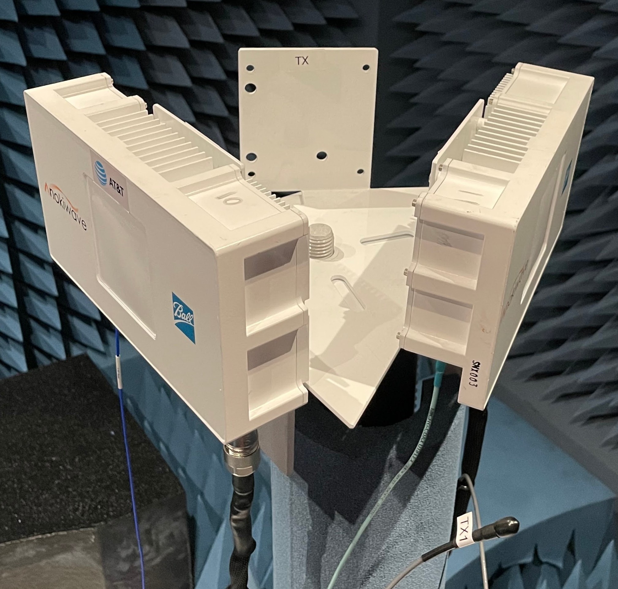
(b) Phased array measurement platform.

Figure 1: (a) A simplified block diagram of our measurement setup using phased arrays to inspect self-interference at 28 GHz. The degree of self-interference depends on the particular choice of transmit beam and receive beam. (b) The phased array measurement platform in an anechoic chamber; receive array on left and transmit array on right.

Our mmWave self-interference measurement system, illustrated as a block diagram in Figure 1a, is comprised of two identical Anokiwave AWA-0134 28 GHz phased array modules [21]: one for transmission and one for reception. Each phased array module consists of a $16\times 16$ half-wavelength UPA, offering high spatial resolution in azimuth and elevation. The transmit and receive arrays were mounted to separate sides of a $60^{\circ}$ equilateral triangular platform, as shown in Figure 1b, where the centers of the arrays were separated by $30$ cm. This configuration aligns with practical, multi-panel (sectorized) full-duplex mmWave deployments, such as for full-duplex IAB as proposed in 3GPP [22]. The measurement platform was placed in an anechoic chamber free from significant reflectors; valuable future work would investigate the impact of reflections.

Each array can be electronically steered by a network of digitally-controlled analog beamforming weights, allowing us to form narrow transmit and receive beams to inspect the directional characteristics of the direct coupling between the transmit and receive arrays. The transmit array is driven by an upconverted 28 GHz Zadoff-Chu sequence with 100 MHz of bandwidth and a power level of $-15$ dBm. The amplified and beamformed transmit signal is radiated by the transmit array at an effective isotropic radiated power (EIRP) of $60$ dBm before coupling over the air with the receive array. The beamformed signal captured by the receive array is internally amplified and downconverted before being digitized. Separate software-defined radio platforms [23] were used to generate signals in the transmit chain and capture signals in the receive chain. In baseband, the transmit and receive signals were processed to estimate the isolation from the input of the transmit array to the output of the receive array. In an effort to more reliably measure isolation, we employed a single Rubidium oscillator and a custom lossless dual upconversion/downconversion system built by Mi-Wave [24]. Correlation-based processing of the Zadoff-Chu signals was used to estimate isolation levels that extend well below the noise floor at the output of our receive array. We calibrated and verified our measurement capability using high-fidelity test equipment [25] and stepped attenuators [26] to ensure our isolation measurements had low error (typically less than $1$ dB) across a broad range of received power levels (roughly from $-20$ dBm to $-110$ dBm). Moreover, we confirmed the repeatability of our measurements in both the short-term (milliseconds) and long-term (minutes).

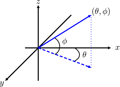
(a) 3-D geometry.

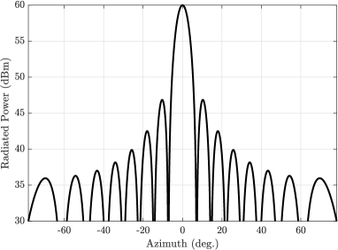
(b) Beam pattern.

Figure 2: (a) The 3-D geometry observed by each phased array. (b) The idealized azimuth radiation pattern of our $16\times 16$ transmit UPA steered broadside. The elevation pattern is identical. The EIRP is $60$ dBm, and the $3$ dB beamwidth is roughly $7^{\circ}$. The pattern of the receive UPA steered broadside is identical.

To describe the arrays’ steering directions in 3-D, we use an azimuth-elevation convention as illustrated in Figure 2a. We assume independent coordinate systems for each array, where each array is centered at the origin facing the positive $x$ axis. From each array’s perspective, broadside corresponds to $0^{\circ}$ in azimuth and elevation (along the positive $x$ axis), upward is an increase in elevation $\phi$ (positive $z$ direction), and rightward (positive $y$ direction) is an increase in azimuth $\theta$. Each array can be independently steered toward a relative azimuth-elevation $(\theta,\phi)$ via beamforming weights. In this work, we employ conjugate beamforming (i.e., matched filter beamforming), where a beam is formed in a particular direction by setting beam weights equal to the conjugate of the array response in that direction. For context, the idealized pattern of a transmit beam steered broadside is shown in Figure 2b, which has a $3$ dB beamwidth of around $7^{\circ}$ in both azimuth and elevation; the shape of a broadside receive beam is identical. Naturally, practical beam patterns will not be as well-defined nor exhibit the deep nulls as that shown in Figure 2b.

The key power levels and power ratios associated with our measurement setup are summarized in Figure 4. When steering the transmit array toward some $(\theta_{\mathrm{tx}},\phi_{\mathrm{tx}})$ and receive array toward $(\theta_{\mathrm{rx}},\phi_{\mathrm{rx}})$, the power of self-interference coupled between the arrays is

$$P_{\mathrm{SI}}\left(\theta_{\mathrm{tx}},\phi_{\mathrm{tx}},\theta_{\mathrm{rx}},\phi_{\mathrm{rx}}\right)=P_{\mathrm{tx}}\cdot L\left(\theta_{\mathrm{tx}},\phi_{\mathrm{tx}},\theta_{\mathrm{rx}},\phi_{\mathrm{rx}}\right)^{-1}$$ (1)

at the receive array output, where $P_{\mathrm{tx}}=-15$ dBm is the power into the transmit array and

$$L\left(\theta_{\mathrm{tx}},\phi_{\mathrm{tx}},\theta_{\mathrm{rx}},\phi_{\mathrm{rx}}\right)=\frac{1}{\left|{\mathbf{w}}\left(\theta_{\mathrm{rx}},\phi_{\mathrm{rx}}\right)^{\mathrm{T}}{\mathbf{H}}{\mathbf{f}}\left(\theta_{\mathrm{tx}},\phi_{\mathrm{tx}}\right)\right|^{2}}$$ (2)

is the effective isolation between the transmit array input and receive array output established by transmit beamforming weights ${\mathbf{f}}$ and receive weights ${\mathbf{w}}$; ${\mathbf{H}}\in\mathbb{C}^{256\times 256}$ is the (unknown) over-the-air self-interference channel matrix between the arrays and has scaling that accounts for the inherent path loss along with transmit and receive gains. In other words, self-interference power $P_{\mathrm{SI}}$ includes the spatial coupling between the transmit and receive beams with the over-the-air channel along with large-scale power gains introduced by the transmit array (e.g., power amplifiers) and receive array (e.g., low noise amplifiers).

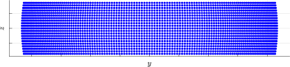
Figure 3: The set of 2,541 transmit directions $\mathcal{A}_{\mathrm{tx}}$ used during measurement, shown here as their respective projections onto the $y$-$z$ plane, where looking into the page represents steering outward from the array (the positive $x$ direction). The set of receive directions $\mathcal{A}_{\mathrm{rx}}$ is identical, densely spanning $-60^{\circ}$ to $60^{\circ}$ in azimuth and $-10^{\circ}$ to $10^{\circ}$ in elevation, each in $1^{\circ}$ steps.

Sets of $N_{\mathrm{tx}}$ transmit directions and $N_{\mathrm{rx}}$ receive directions

$$\mathcal{A}_{\mathrm{tx}} =\left\{\left(\theta_{\mathrm{tx}}^{\left(i\right)},\phi_{\mathrm{tx}}^{\left(i\right)}\right)\right\}_{i=1}^{N_{\mathrm{tx}}},\qquad\mathcal{A}_{\mathrm{rx}}=\left\{\left(\theta_{\mathrm{rx}}^{\left(j\right)},\phi_{\mathrm{rx}}^{\left(j\right)}\right)\right\}_{j=1}^{N_{\mathrm{rx}}}$$ (3)

are specified prior to executing our measurement campaign. We measure the self-interference power between each transmit and receive steering combination for a total of $N_{\mathrm{tx}}\times N_{\mathrm{rx}}$ measurements. Depicted in Figure 3, the results in this work are based on measurements whose transmit and receive directions are each distributed uniformly in azimuth from $-60^{\circ}$ to $60^{\circ}$ with $1^{\circ}$ spacing and in elevation from $-10^{\circ}$ to $10^{\circ}$ with $1^{\circ}$ spacing. This amounts to $N_{\mathrm{tx}}=N_{\mathrm{rx}}=121\times 21=2541$ directions for transmission and for reception, totaling $2541\times 2541\approx 6.5$ million self-interference power measurements.

Figure 4: A summary of the key power levels and power ratios associated with our measurement system.

Referencing the measured self-interference power $P_{\mathrm{SI}}$ to the noise floor of the receive array, the INR for given transmit and receive directions can be written as

$$\mathsf{INR}\left(\theta_{\mathrm{tx}},\phi_{\mathrm{tx}},\theta_{\mathrm{rx}},\phi_{\mathrm{rx}}\right)=\frac{P_{\mathrm{SI}}\left(\theta_{\mathrm{tx}},\phi_{\mathrm{tx}},\theta_{\mathrm{rx}},\phi_{\mathrm{rx}}\right)}{P_{\mathrm{noise}}}$$ (4)

where $P_{\mathrm{noise}}=-68$ dBm is the noise power at the receive array output over $100$ MHz. INR is an important quantity for describing if a full-duplex system is self-interference-limited ($\mathsf{INR}\gg 0$ dB), noise-limited ($\mathsf{INR}\ll 0$ dB), or somewhere in between. For full-duplex, we desire low $\mathsf{INR}$, roughly $\mathsf{INR}\leq 0$ dB in most cases, to ensure self-interference does not erode full-duplexing gain. The set of all nearly 6.5 million measured INR values we write as

$$\mathcal{I}=\left\{\mathsf{INR}\left(\theta_{\mathrm{tx}},\phi_{\mathrm{tx}},\theta_{\mathrm{rx}},\phi_{\mathrm{rx}}\right):\left(\theta_{\mathrm{tx}},\phi_{\mathrm{tx}}\right)\in\mathcal{A}_{\mathrm{tx}},\left(\theta_{\mathrm{rx}},\phi_{\mathrm{rx}}\right)\in\mathcal{A}_{\mathrm{rx}}\right\}$$ (5)

and refer to the INR measured when transmitting with the $i$-th transmit beam and receiving with the $j$-th receive beam as

$$\mathsf{INR}_{ij}=\mathsf{INR}\left(\theta_{\mathrm{tx}}^{\left(i\right)},\phi_{\mathrm{tx}}^{\left(i\right)},\theta_{\mathrm{rx}}^{\left(j\right)},\phi_{\mathrm{rx}}^{\left(j\right)}\right).$$ (6)

A desired signal having received power $P_{\mathrm{des}}$ (at the output of the receive array) would see a signal-to-interference-plus-noise ratio (SINR) of

$$\mathsf{SINR}\left(\theta_{\mathrm{tx}},\phi_{\mathrm{tx}},\theta_{\mathrm{rx}},\phi_{\mathrm{rx}}\right) =\frac{P_{\mathrm{des}}}{P_{\mathrm{noise}}+P_{\mathrm{SI}}\left(\theta_{\mathrm{tx}},\phi_{\mathrm{tx}},\theta_{\mathrm{rx}},\phi_{\mathrm{rx}}\right)}=\frac{\mathsf{SNR}}{1+\mathsf{INR}\left(\theta_{\mathrm{tx}},\phi_{\mathrm{tx}},\theta_{\mathrm{rx}},\phi_{\mathrm{rx}}\right)}$$ (7)

where $\mathsf{SNR}$ is the signal-to-noise ratio (SNR) of the desired signal. Notice that $\mathsf{SINR}$ depends on the level of self-interference incurred when steering the transmitter toward $(\theta_{\mathrm{tx}},\phi_{\mathrm{tx}})$ and the receiver toward $(\theta_{\mathrm{rx}},\phi_{\mathrm{rx}})$; of course, $\mathsf{SNR}$ would practically also be a function of $(\theta_{\mathrm{rx}},\phi_{\mathrm{rx}})$. This work is solely concerned with measuring $\mathsf{INR}$ (self-interference), from which desired signals having some $\mathsf{SNR}$ can be evaluated in a full-duplex sense. We would like to point out that all measurements collected in this campaign are for a fixed setup as described; valuable future work would investigate the impact of system parameters such as beam shape (e.g., beamwidth and side lobe levels), array sizes, and panel geometries.

III High-Level Summary and Spatial Insights

Perhaps the best summary of our measurements is the cumulative density function (CDF) of the nearly 6.5 million measured INR values in Figure 5. The maximum and minimum measured INR were nearly $46.99$ dB and $-44.57$ dB, respectively. The measured INR typically falls between $0$ dB and $40$ dB, with median INR at $20.27$ dB. Nearly $99$% of beam pairs offer an INR greater than $0$ dB, where self-interference power exceeds noise power. Around $90$% of beam pairs yield an $\mathsf{INR}\geq 10$ dB, where self-interference is at least ten times as strong as noise. Just over $2$% of beam pairs offer an $\mathsf{INR}\leq 3$ dB. Naturally, this CDF of $\mathsf{INR}$ would shift left/right if transmit power were to decrease/increase or noise power were to increase/decrease, for instance; those wishing to appropriately translate our measurements to systems with different power levels can refer to Figure 4.

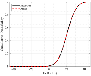
Figure 5: The CDF of the nearly 6.5 million measured INR values and its fitted log-normal distribution.

Takeaways.

At first glance, the CDF of the measured $\mathsf{INR}$ values seems quite pessimistic from a full-duplex perspective, considering most beam pairs yield self-interference levels that are well above the noise floor. Multi-panel full-duplex mmWave systems similar to ours will typically be overwhelmed with self-interference when choosing a random transmit and receive beam, motivating the need for additional means to reduce self-interference. Nonetheless, it is a welcome sight to observe that there exist select beam pairs that do in fact offer INR levels sufficiently low for full-duplex—we explore the directional nature of these beam pairs shortly in Subsection III-B. Valuable future work would explore solutions to reduce self-interference and investigate how system design choices can potentially reduce INR levels while maintaining service to users.

We found that the CDF in Figure 5 can be well approximated by a log-normal distribution, shown as a dashed line in Figure 5. That is to say that the measured INR values in dB approximately follow a normal distribution as

$$\left[\mathcal{I}\right]_{\mathrm{dB}}\overset{\mathrm{fit}}{\sim}\mathcal{N}\left(\mu,\sigma^{2}\right)$$ (8)

where $\mu=20.32$ and $\sigma^{2}=70.69$ are the fitted mean and variance of the normal distribution. Like the CDF in Figure 5, changes to large-scale parameters that impact INR—such as the transmit power or noise power—can be accounted for in $\mu$ to shift the fitted normal distribution left or right. Albeit limited, engineers can make first-order statistical approximations of self-interference via this log-normal distribution when drawing independently and identically distributed (i.i.d.) INR values as $\left[\mathsf{INR}\right]_{\mathrm{dB}}\sim\mathcal{N}\left(\mu,\sigma^{2}\right)$. For instance, the probability that the INR of a random transmit-receive beam pair will fall below $\gamma$ (in linear units) can be well approximated as

$$\mathbb{P}\left(\mathsf{INR}\leq\gamma\right)=\frac{1}{2}\left[1+\mathrm{erf}\left(\frac{\left[\gamma\right]_{\mathrm{dB}}-\mu}{\sigma\cdot\sqrt{2}}\right)\right].$$ (9)

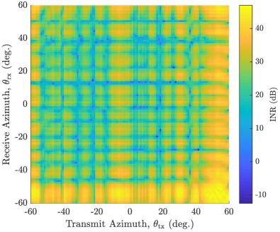
(a) Measured INR.

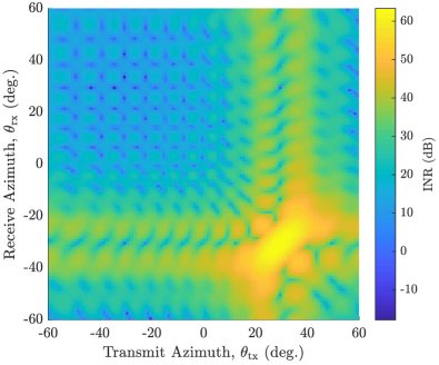
(b) Simulated INR with spherical-wave channel.

Figure 6: (a) Measured INR as a function of azimuthal transmit and receive directions when $\phi_{\mathrm{tx}}=\phi_{\mathrm{rx}}=0^{\circ}$. (b) The simulated counterpart of (a) when using a spherical-wave near-field self-interference channel model [18], which clearly does not align well with what was measured. This motivates the need for a new, measurement-backed channel model for mmWave self-interference.

III-A Is an Idealized Near-Field Self-Interference Channel Model Realistic?

A natural question to ask before proceeding is if the aforementioned spherical-wave MIMO channel model [18]—an idealized near-field propagation model—aligns with our measurements. If it does, self-interference power values could be realized deterministically via the product of transmit and receive beamforming weights ${\mathbf{f}}$ and ${\mathbf{w}}$ with a MIMO channel matrix ${\mathbf{H}}$ based on the spherical-wave model. Unfortunately, however, we found that the spherical-wave MIMO channel model does not align with our measurements. Consider Figure 6, where we plot the measured INR values across the azimuth plane and the simulated counterpart using the spherical-wave MIMO channel model. Notice that the two are starkly different, indicating that this idealized near-field channel model—which has been used so frequently as a means to evaluate mmWave full-duplex—does not translate to practical systems, which pose a number of nonidealities stemming from array enclosures, mounting infrastructure, and non-isotropic antenna elements, for instance. This motivates the need for a practical, measurement-backed MIMO channel model for mmWave self-interference, which we plan to address in future work.

III-B Maximum, Median, and Minimum INR for Particular Transmit Beams and Receive Beams

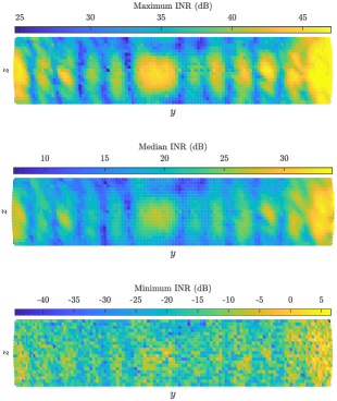
(a) Observed by each transmit beam.

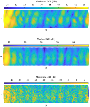
(b) Observed by each receive beam.

Figure 7: For each transmit beam and receive beam, shown are the maximum, median, and minimum INR across all receive and transmit beams, respectively.

The CDF in Figure 5 and its corresponding fitted distribution are certainly useful statistically but do not provide any spatial insight on self-interference. As such, we now hone in on narrower perspectives to better visualize and interpret our measurements spatially. First, let us begin by considering Figure 7a, which shows the maximum, median, and minimum INR observed by each transmit beam across all receive beams; each dot corresponds to a transmit beam’s projection onto the $y$-$z$ plane (i.e., its direction from the perspective of the transmit array). In other words, the maximum INR observed by the $i$-th transmit beam (the $i$-th dot) is simply $\max_{j}\mathsf{INR}_{ij}$, for example, with median and minimum expressed analogously. Figure 7b similarly shows these statistics observed when receiving a particular direction. Referencing Figure 7b, we can see that the median INR per receive beam ranges from approximately $8$ dB to $35$ dB. The maximum INR observed at each receive beam is at least around $28$ dB and at most over $46$ dB, while the minimum INR is at least around $-45$ dB and at most around $7$ dB. In a similar fashion, we examine these statistics for each transmit beam in Figure 7a, which tell a similar story both visually and numerically as the receive side.

Takeaways.

There are a few important things to take away from Figure 7a and Figure 7b. As intuition may suggest based on Figure 1b, the results of Figure 7a and Figure 7b indicate that:

• transmitting to toward the receiver tends to couple more self-interference

• receiving toward the transmitter tends to couple more self-interference.

Considering minimum INR is at most around $7$ dB in both, we see that (i) even when steering our transmitter toward the receiver, there exist some receive beam(s) that offer low INR (at most around $7$ dB) and (ii) even when steering our receiver toward the transmitter, there exist some transmit beam(s) that offer low INR (at most around $7$ dB). This suggests that—while transmitting toward the receiver and receiving toward the transmitter generally results in more self-interference—there exist receive beams and transmit beams that can offer low INR. In Section IV, we observe that low-INR beam pairs appear to be distributed throughout space. We have ongoing work that investigates if these low-INR beam pairs can in fact be used to serve users with high beamforming gain while simultaneously offering reduced self-interference, facilitating full-duplex operation. In a similar fashion, observing maximum INR illustrates that there also consistently exists transmit-receive combinations that can lead to high self-interference. From this, we can conclude that there are not transmit beams nor receive beams that universally offer low or high INR—though there exist those that tend to. Rather, the amount of self-interference coupled depends heavily on one’s choice of transmit beam and receive beam.

Takeaways.

Additional takeaways include the fact that we observe strong similarities between the transmit and receive profiles, which validates some degree of channel symmetry. However, there do exist noteworthy differences, particularly the strong self-interference present when transmitting around broadside but not when receiving. The high self-interference coupled when transmitting around broadside is not necessarily expected nor easily explained; it can perhaps be attributed to coupling behind the arrays due to mounting hardware and array enclosures. Also, we see significantly more variation across $y$ than $z$, suggesting that the azimuth of the steering direction plays a greater role than elevation, which one may expect since our transmitter and receiver are separated in azimuth but not in elevation. While it may seem obvious that transmitting toward the receiver and receiving toward the transmitter would couple the most self-interference, it was not clear that this would be the case since the transmit and receive arrays exist in the near-field of one another. The far-field distance of our arrays is approximately $2.4$ meters based on the rule-of-thumb $2D^{2}/\lambda$ [27], while our arrays are separated by only $30$ cm. The reactive/radiating near-field boundary, on the other hand, is around a mere $23$ cm based on the rule-of-thumb $0.62\sqrt{D^{3}/\lambda}$ [27], suggesting that our arrays live just within the radiating near-field of one another. Operating in this near-field regime, the highly directional beams created by our UPAs are not necessarily “highly directional” from the perspective of one another [1].

III-C Meeting INR Thresholds with Particular Transmit Beams and Receive Beams

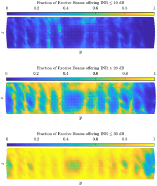
(a) Observed by each transmit beam.

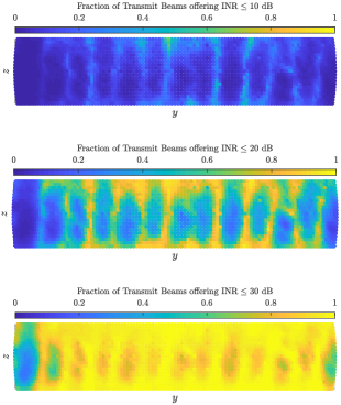
(b) Observed by each receive beam.

Figure 8: For each transmit beam and receive beam, shown is the fraction of receive beams and transmit beams, respectively, that meet various INR thresholds.

Having looked at the maximum, median, and minimum INR for particular transmit beams and receive beams, we now examine the fraction of beams that offer certain levels of INR. In Figure 8a, for each transmit beam, we look at the fraction of receive beams that offer at most $10$ dB, $20$ dB, and $30$ dB of INR. Similarly, in Figure 8b, for each receive beam, we look at the fraction of transmit beams that offer these same levels of INR. From the top plot of each, we see that a modest INR threshold of $10$ dB (where self-interference is ten times stronger than noise) cannot be met very reliably by any transmit beam nor any receive beam. At best, select beams can only meet this target INR around $50$% of the time, with the vast majority falling quite short of this. Naturally, as the INR threshold rises to $20$ dB, the fraction of beams that can meet this threshold increases. Transmit and receive options emerge that offer an INR of at most $20$ dB over $50$% of the time, with some approaching $100$%. Still, however, the transmit beams steering rightward toward the receiver and the receive beams steering leftward toward the transmitter struggle to offer an INR below $20$ dB. Increasing the INR threshold further, nearly all transmit and receive beams can confidently offer an INR within $30$ dB, though those least likely to do so are the rightward transmit beams, leftward receive beams, and broadside transmit beams.

Takeaways.

The most promising transmit beams and receive beams in meeting an INR threshold of $20$ dB, for example, can be seen as thin vertical strips of bright yellow. These vertical strips, which were also visible as low-INR beams in Figure 7, are likely attributed to nulls in the transmit and receive beam patterns. Notice, however, since the statistics of Figure 8 were taken over all transmit/receive beams, it shows that the transmit nulls are robust to some degree, somewhat reliably offering lower INR regardless of the receive beam being used (and vice versa). These transmit and receive beams offering lower INR across large fractions of receive beams and transmit beams, respectively, correspond to the approximate transmit and receive nulls at the channel input and output (i.e., approximate right and left null spaces of ${\mathbf{H}}$), respectively. Recall, from Figure 7a and Figure 7b, we did not see any transmit beams or receive beams that universally provided high isolation. If indeed these vertical strips are attributed to nulls in the beam patterns, this suggests that the self-interference channel between the transmit and receive arrays is quite directional, which somewhat further bucks the thought that near-field interaction dominates their coupling. Our future work will explore this to better understand the coupling nature of the arrays.

III-D INR for Particular Transmit-Receive Beam Pairs

Honing in further, we now look at the isolation achieved at each transmit beam for a particular receive beam and at each receive beam for a particular transmit beam, as shown in Figure 9a and Figure 9b. Let us first consider the INR observed across receive beams for particular transmit beams; imagine fixing the transmit beam and sweeping the receive beam to measure INR at each. In Figure 9b, we have selected two transmit directions: toward the receive array (top plot) and away from the receive array (bottom plot). For each, have shown the INR measured between the transmit beam and each receive beam option. Shown in the top plot of Figure 9b, when transmitting rightward toward the receiver (whose direction is shown as a red circle), we see fairly high INR across the receive profile. Large orange/yellow spots make up most of the receive profile, highlighting just how difficult it may be to find a receive beam that offers low INR for this particular transmit beam. There exist some low-INR receive options narrowly in between large spots of orange or at high and low elevation.

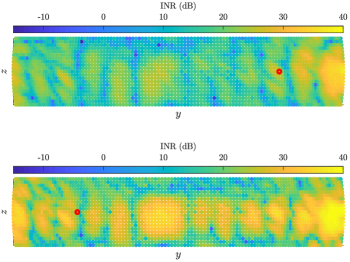
(a) Observed by each transmit beam.

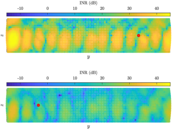
(b) Observed by each receive beam.

Figure 9: For each transmit beam and receive beam, shown is the measured INR across all receive and transmit beams, respectively. The red circle indicates the (a) receive direction and (b) transmit direction.

Now, looking at the bottom plot of Figure 9b, when steering the transmitter leftward away from the receiver, the INR profile across receive beams expectedly changes. The INR profile sees a widespread decrease of about $10$ dB or more and options for extremely low INR are more available. Still, receiving leftward toward the transmitter remains the least attractive option and reinforces that isolation may tend to be lower when transmitting rightward toward the receiver and when receiving leftward toward the transmitter—but this is not universally the case. Looking at both plots in Figure 9b, the receive beam that offers minimum INR varies with transmit beam, which further backs our claim that there are not receive beams that universally offer low INR. Moreover, the low-INR receive directions are typically quite narrow in the sense that small changes in receive direction can lead to significant changes in isolation. For instance, when transmitting rightward toward the receiver, the INR across receive beams varies by about $60$ dB, and we see that shifting a receive beam by only $1^{\circ}$ to $2^{\circ}$ in azimuth and/or elevation can lead to changes of $20$–$30$ dB or more in INR. Notice that this sensitivity to steering direction is much more apparent with low-INR beams than high-INR ones.

Similarly, in Figure 9a, we have selected two receive directions and, for each, have shown the INR measured between the receive beam and each transmit beam. Analogous conclusions can be drawn as with Figure 9b, though there are useful comments to make. Again, varying with each receive beam, there exists an INR-minimizing transmit beam. Notice that even when the receive beam is steered away from the transmit array (to the right; top plot), transmitting toward the receive array (to the right) still inflicts substantial self-interference. We can clearly see that simply steering the transmitter away from the receiver or steering the receiver away from the transmitter does not offer widespread low INR. Comparing Figure 9a and Figure 9b, we observe a certain degree of symmetry. Transmitting toward the receiver (top Figure 9b) is similar to receiving toward the transmitter (bottom Figure 9a). Transmitting away from the receiver (bottom Figure 9b) is similar to receiving away from the transmitter (top Figure 9a). This further verifies a sense of spatial symmetry of our self-interference channel ${\mathbf{H}}$.

Takeaways.

Figure 9a and Figure 9b highlight that there exist large-scale (global) trends in the amount of self-interference coupled between the transmit and receive arrays, since general steering direction of the transmitter and receiver can play a significant role in the INR profile. In addition, they also illustrate the local phenomena present in the INR profile: small shifts in steering direction can have drastic impacts on the degree of self-interference coupled. Figure 9a and Figure 9b showed this sensitivity of the transmit beam and receive beam separately—in the next section, we investigate this sensitivity when the transmit beam and receive beam both see small shifts in their steering direction.

IV Quantifying the Angular Spread of mmWave Self-Interference

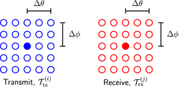
Figure 10: The transmit and receive steering neighborhoods $\mathcal{T}_{\mathrm{tx}}^{\left(i\right)}$ and $\mathcal{T}_{\mathrm{rx}}^{\left(j\right)}$, where the filled circles indicate the nominal steering directions $\left(\theta_{\mathrm{tx}}^{\left(i\right)},\phi_{\mathrm{tx}}^{\left(i\right)}\right)$ and $\left(\theta_{\mathrm{rx}}^{\left(j\right)},\phi_{\mathrm{rx}}^{\left(j\right)}\right)$ and the unfilled circles indicate directions comprising the $\left(\Delta\theta,\Delta\phi\right)$-neighborhood surrounding each. In this case, the $25$ directions in each yields $25^{2}=625$ transmit-receive steering combinations.

In this section, we inspect how self-interference varies with small changes in transmit and receive directions. Let us begin by defining $\measuredangle\left(\alpha,\beta\right)$ as the absolute difference between two angles $\alpha,\beta$ (in degrees), written as

$$\measuredangle\left(\alpha,\beta\right)=\begin{cases}\zeta,&\zeta\leq 180^{\circ}\\ 360^{\circ}-\zeta,&\zeta>180^{\circ}\\ \end{cases}$$ (10)

where $\zeta=\left|\alpha-\beta\right|\ \mathrm{mod}\ 360^{\circ}$ and $\mathrm{mod}$ is the modulo operator. Let $\mathcal{T}_{\mathrm{tx}}^{\left(i\right)}$ and $\mathcal{T}_{\mathrm{rx}}^{\left(j\right)}$ be the $(\Delta\theta,\Delta\phi)$-neighborhoods around the $i$-th transmit direction and $j$-th receive direction, respectively, defined as

$$\mathcal{T}_{\mathrm{tx}}^{\left(i\right)}\left(\Delta\theta,\Delta\phi\right) =\left\{(\theta,\phi)\in\mathcal{A}_{\mathrm{tx}}:\measuredangle\left(\theta,\theta_{\mathrm{tx}}^{\left(i\right)}\right)\leq\Delta\theta,\measuredangle\left(\phi,\phi_{\mathrm{tx}}^{\left(i\right)}\right)\leq\Delta\phi\right\}$$ (11)

$$\mathcal{T}_{\mathrm{rx}}^{\left(j\right)}\left(\Delta\theta,\Delta\phi\right) =\left\{(\theta,\phi)\in\mathcal{A}_{\mathrm{rx}}:\measuredangle\left(\theta,\theta_{\mathrm{rx}}^{\left(j\right)}\right)\leq\Delta\theta,\measuredangle\left(\phi,\phi_{\mathrm{rx}}^{\left(j\right)}\right)\leq\Delta\phi\right\}$$ (12)

and illustrated in Figure 10. For some $(\Delta\theta,\Delta\phi)$ in degrees, the cardinality of these sets is

$$\left|\mathcal{T}_{\mathrm{tx}}^{\left(i\right)}\left(\Delta\theta,\Delta\phi\right)\right|,\left|\mathcal{T}_{\mathrm{rx}}^{\left(j\right)}\left(\Delta\theta,\Delta\phi\right)\right|\leq(2\cdot\Delta\theta+1)\cdot(2\cdot\Delta\phi+1)$$ (13)

with equality when not at the edge of the measurement space (which is typical); the crude use of $\Delta\theta$ and $\Delta\phi$ here is thanks to our $1^{\circ}$ spacing of $\mathcal{A}_{\mathrm{tx}}$ and $\mathcal{A}_{\mathrm{rx}}$.

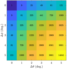
Figure 11: The number of transmit-receive beam pairs for a typical $\left(\Delta\theta,\Delta\phi\right)$-neighborhood under our $\left(1^{\circ},1^{\circ}\right)$ resolution.

Then, let $\mathcal{I}_{ij}(\Delta\theta,\Delta\phi)$ be the set of measured INR values across the $(\Delta\theta,\Delta\phi)$-neighborhood surrounding the $(i,j)$-th transmit-receive beam pair, expressed as

$$\mathcal{I}_{ij}(\Delta\theta,\Delta\phi)=\left\{\mathsf{INR}(\theta_{\mathrm{tx}},\phi_{\mathrm{tx}},\theta_{\mathrm{rx}},\phi_{\mathrm{rx}}):\left(\theta_{\mathrm{tx}},\phi_{\mathrm{tx}}\right)\in\mathcal{T}_{\mathrm{tx}}^{\left(i\right)}\left(\Delta\theta,\Delta\phi\right),\left(\theta_{\mathrm{rx}},\phi_{\mathrm{rx}}\right)\in\mathcal{T}_{\mathrm{rx}}^{\left(j\right)}\left(\Delta\theta,\Delta\phi\right)\right\}$$ (14)

where $\mathcal{T}_{\mathrm{tx}}^{\left(i\right)}$ and $\mathcal{T}_{\mathrm{rx}}^{\left(j\right)}$ depends on the beam pair $(i,j)$ and neighborhood size $(\Delta\theta,\Delta\phi)$. As the $(\Delta\theta,\Delta\phi)$-neighborhoods are widened, the cardinality of $\mathcal{I}_{ij}$ grows, which is simply the product of that of $\mathcal{T}_{\mathrm{tx}}^{\left(i\right)}$ and $\mathcal{T}_{\mathrm{rx}}^{\left(j\right)}$.

$$\left|\mathcal{I}_{ij}(\Delta\theta,\Delta\phi)\right|=\left|\mathcal{T}_{\mathrm{tx}}^{\left(i\right)}\left(\Delta\theta,\Delta\phi\right)\right|\cdot\left|\mathcal{T}_{\mathrm{rx}}^{\left(j\right)}\left(\Delta\theta,\Delta\phi\right)\right|$$ (15)

Based on (13), the upper bound of (15) is tabulated for various $\left(\Delta\theta,\Delta\phi\right)$ in Figure 11, which grows with order $\mathcal{O}\left(\Delta\theta^{2}\cdot\Delta\phi^{2}\right)$.

The minimum INR and maximum INR offered by beam pairs across the $(\Delta\theta,\Delta\phi)$-neighborhood surrounding the $(i,j)$-th beam pair can be expressed as simply

$$\mathsf{INR}_{ij}^{\mathrm{min}}(\Delta\theta,\Delta\phi) =\min\left\{\mathcal{I}_{ij}(\Delta\theta,\Delta\phi)\right\}$$ (16)

$$\mathsf{INR}_{ij}^{\mathrm{max}}(\Delta\theta,\Delta\phi) =\max\left\{\mathcal{I}_{ij}(\Delta\theta,\Delta\phi)\right\}.$$ (17)

Using these, the INR range (in dB) we define as

$$\mathsf{INR}_{ij}^{\mathrm{rng}}(\Delta\theta,\Delta\phi)=\left[\mathsf{INR}_{ij}^{\mathrm{max}}(\Delta\theta,\Delta\phi)\right]_{\mathrm{dB}}-\left[\mathsf{INR}_{ij}^{\mathrm{min}}(\Delta\theta,\Delta\phi)\right]_{\mathrm{dB}}\geq 0$$ (18)

which captures how much the INR can vary over the $(\Delta\theta,\Delta\phi)$-neighborhood surrounding the $(i,j)$-th beam pair. By examining $\mathsf{INR}_{ij}^{\mathrm{min}}\left(\Delta\theta,\Delta\phi\right)$, $\mathsf{INR}_{ij}^{\mathrm{max}}\left(\Delta\theta,\Delta\phi\right)$, and $\mathsf{INR}_{ij}^{\mathrm{rng}}\left(\Delta\theta,\Delta\phi\right)$ for each transmit-receive steering combination $(i,j)$ and for variably sized neighborhoods, we can gain insight into the angular spread of self-interference. We point out that, since our measurements were taken with $1^{\circ}$ resolution in azimuth and elevation, there exists the potential to see greater INR range, lower minimum INR, and/or higher maximum INR if sub-$\left(1^{\circ},1^{\circ}\right)$ resolutions were used; as such, the results herein can be considered a potentially conservative measure on these statistics over small neighborhoods.

IV-A INR Range over Various Neighborhoods

In Figure 12a, we plot the CDF of INR range for variably sized $\left(\Delta\theta,\Delta\phi\right)$-neighborhoods across all measured direction pairs (i.e., each CDF contains nearly 6.5 million points). As shown in Figure 12a, moving a beam pair by only $1^{\circ}$ in either azimuth or elevation can lead to notable changes in INR: around $25$% of beam pairs observe over $10$ dB of INR range in either case. As the neighborhood size increases, we naturally observe a wider range of INR. $50$% of beam pairs see more than $17$ dB of variability in INR across a $(1^{\circ},1^{\circ})$-neighborhood. In other words, if we consider a beam pair at random and look around its $(1^{\circ},1^{\circ})$-neighborhood, we would expect the INR to vary by $17$ dB or more. Across a $(2^{\circ},2^{\circ})$-neighborhood, $80$% of beam pairs see around $25$ dB or more of variability in INR. Notice that there exists slightly more variability in INR across azimuth than across elevation, evidenced by the $\left(1^{\circ},0^{\circ}\right)$- and $\left(0^{\circ},1^{\circ}\right)$-neighborhoods—perhaps due to the horizontal separation of our transmit and receive arrays.

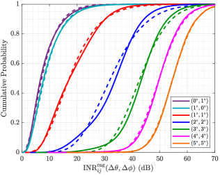
(a) $\mathsf{INR}_{ij}^{\mathrm{rng}}(\Delta\theta,\Delta\phi)$.

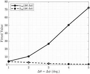
(b) $\alpha_{\mathrm{rng}}(\Delta\theta,\Delta\phi)$ and $\beta_{\mathrm{rng}}(\Delta\theta,\Delta\phi)$.

Figure 12: (a) The CDF of $\mathsf{INR}_{ij}^{\mathrm{rng}}$ across all nearly 6.5 million transmit-receive beam pairs for various neighborhood sizes $(\Delta\theta,\Delta\phi)$. Fitted distributions for each are shown as dashed lines. (b) The fitted parameters $\alpha_{\mathrm{rng}}(\Delta\theta,\Delta\phi)$ and $\beta_{\mathrm{rng}}(\Delta\theta,\Delta\phi)$ for various $\Delta\theta=\Delta\phi$.

To provide engineers with statistics on $\mathsf{INR}_{ij}^{\mathrm{rng}}$ for variably sized $(\Delta\theta,\Delta\phi)$-neighborhoods, we have fit a distribution to $\left\{\mathsf{INR}_{ij}^{\mathrm{rng}}(\Delta\theta,\Delta\phi)\right\}$. Specifically, we found that a Gamma distribution can be fitted to each of the CDFs in Figure 12a as follows

$$\left\{\left[\mathsf{INR}_{ij}^{\mathrm{rng}}(\Delta\theta,\Delta\phi)\right]_{\mathrm{dB}}\ \forall\ i,j\right\}\overset{\mathrm{fit}}{\sim}\mathrm{Gamma}\left(\alpha_{\mathrm{rng}}(\Delta\theta,\Delta\phi),\beta_{\mathrm{rng}}(\Delta\theta,\Delta\phi)\right)$$ (19)

where $\alpha_{\mathrm{rng}}(\Delta\theta,\Delta\phi)>0$ and $\beta_{\mathrm{rng}}(\Delta\theta,\Delta\phi)>0$ are the fitted shape and rate (inverse scale) of the Gamma distribution. The fitted Gamma distributions for each neighborhood in Figure 12a are shown as dashed lines. In addition, we have plotted $\alpha_{\mathrm{rng}}\left(\Delta\theta,\Delta\phi\right)$ and $\beta_{\mathrm{rng}}\left(\Delta\theta,\Delta\phi\right)$ as functions of $\Delta\theta=\Delta\phi$ in Figure 12b. As $\Delta\theta=\Delta\phi$ increases, the shape parameter $\alpha_{\mathrm{rng}}$ drastically increases and the rate parameter $\beta_{\mathrm{rng}}$ decays toward zero, which is a reflection of the CDFs in Figure 12a shifting rightward.

In addition to those shown in Figure 12, we fitted unique Gamma distributions for $\Delta\theta,\Delta\phi\in\left\{0^{\circ},1^{\circ},\dots,5^{\circ}\right\}$ and tabulated the fitted parameters $(\alpha_{\mathrm{rng}}\left(\Delta\theta,\Delta\phi\right),\beta_{\mathrm{rng}}\left(\Delta\theta,\Delta\phi\right))$ for each in Table I. Engineers wishing to realize the range in INR over a random $\left(\Delta\theta,\Delta\phi\right)$-neighborhood or conduct statistical analyses related to such can refer to Table I for adequate Gamma distribution parameters $(\alpha_{\mathrm{rng}}\left(\Delta\theta,\Delta\phi\right),\beta_{\mathrm{rng}}\left(\Delta\theta,\Delta\phi\right))$. Then, the expected range in $\mathsf{INR}$ (in dB) over some $\left(\Delta\theta,\Delta\phi\right)$-neighborhood, for instance, can be approximated as simply

$$\mathbb{E}\left[\mathsf{INR}_{ij}^{\mathrm{rng}}\left(\Delta\theta,\Delta\phi\right)\right]=\frac{\alpha_{\mathrm{rng}}\left(\Delta\theta,\Delta\phi\right)}{\beta_{\mathrm{rng}}\left(\Delta\theta,\Delta\phi\right)}$$ (20)

based on the Gamma distribution, along with an assortment of other statistics readily computed.

Takeaways.

Figure 12a highlights that the self-interference channel is not spatially smooth. Rather, small changes in steering direction can result in significant changes in the degree of self-interference coupled and, hence, significant changes in full-duplex performance. As such, mmWave full-duplex systems cannot expect to reliably avoid self-interference by broadly steering transmit and receive beams. Instead, transmit and receive beams will need to be carefully (and jointly) steered, as small errors in steering direction can lead to drastic changes in self-interference.

IV-B Minimum INR over Various Neighborhoods

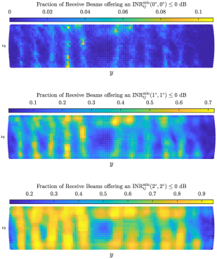
(a) Observed by each transmit beam.

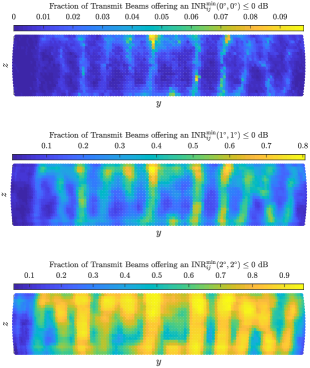
(b) Observed by each receive beam.

Figure 13: For each transmit beam and receive beam, shown are the fraction of receive beams and transmit beams, respectively, that can offer an INR of $0$ dB or less when allowed to deviate by various $\left(\Delta\theta,\Delta\phi\right)$. Low INR becomes reliably within arm’s reach by increasing $\left(\Delta\theta,\Delta\phi\right)$.

Now, we examine the minimum INR that can be reached by each beam pair if allowed to deviate around some spatial neighborhood. To illustrate this, we have included Figure 13. In Figure 13a, at each transmit beam, we show the fraction of receive beams that can offer a minimum INR of $0$ dB or less. We do this for various neighborhood sizes $\left(\Delta\theta,\Delta\phi\right)$, where a $\left(0^{\circ},0^{\circ}\right)$-neighborhood is simply no deviation. With a $\left(0^{\circ},0^{\circ}\right)$-neighborhood, most transmit-receive beams cannot meet the INR threshold of $0$ dB. As the neighborhood grows to $\left(1^{\circ},1^{\circ}\right)$, we see that, for some transmit beams, a large fraction of receive beams can reach an INR of $0$ dB (and vice versa). With $\left(2^{\circ},2^{\circ}\right)$ of freedom, we see the clouds of yellow grow as more receive beams offer an INR of $0$ dB for even more transmit beams. Figure 13 illustrates the significant changes observed in INR due to slight shifts of the transmit and receive beams and shows that INR levels suitable for full-duplex are in fact within arm’s reach.

Consider Figure 14a, where we plot the CDF of $\left\{\mathsf{INR}_{ij}^{\mathrm{min}}\right\}$ for variably sized $\left(\Delta\theta,\Delta\phi\right)$-neighborhoods across all measured beam pairs. The dashed black line in Figure 14a is simply the CDF of $\left\{\mathsf{INR}_{ij}\right\}$ for each beam pair since $\Delta\theta=\Delta\phi=0^{\circ}$ (shown previously in Figure 5). When considering small neighborhoods around each beam pair, however, much more promising results are observed. When shifting beams by no more than $1^{\circ}$ in azimuth and elevation, the probability of reaching $\mathsf{INR}\leq 0$ dB (where self-interference is no stronger than noise) grows to over $25$% from around $1$%. With $2^{\circ}$, it grows to over $65$%; that is to say that over $65$% of beam pairs are within $(2^{\circ},2^{\circ})$ of a beam pair that offers $\mathsf{INR}\leq 0$ dB.

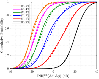
(a) $\mathsf{INR}_{ij}^{\mathrm{min}}(\Delta\theta,\Delta\phi)$.

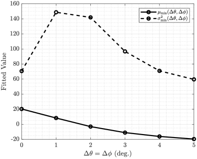
(b) $\mu_{\mathrm{min}}(\Delta\theta,\Delta\phi)$ and $\sigma^{2}_{\mathrm{min}}(\Delta\theta,\Delta\phi)$.

Figure 14: (a) The CDF of $\mathsf{INR}_{ij}^{\mathrm{min}}(\Delta\theta,\Delta\phi)$ for various $(\Delta\theta,\Delta\phi)$. For each, the fitted distribution is shown as a dashed line. (b) The fitted parameters $\mu_{\mathrm{min}}(\Delta\theta,\Delta\phi)$ and $\sigma^{2}_{\mathrm{min}}(\Delta\theta,\Delta\phi)$ for various $\Delta\theta=\Delta\phi$.

Takeaways.

Clearly, INR can be greatly improved with slight shifts in the steering directions of the transmit and/or receive beams. From this, we draw an important conclusion: steering directions that do not inherently offer high isolation (i.e., low $\mathsf{INR}_{ij}$) are likely spatially near ones that do. These are highly encouraging results for the potential of mmWave full-duplex since they suggest that self-interference can be greatly reduced while making very minor adjustments to the transmit and receive steering directions. This is reinforced further by the fact that our beams have a $3$ dB beamwidth around $7^{\circ}$, meaning slight deviations will hopefully not sacrifice too much beamforming gain when making these adjustments. To reach these low-INR beam pairs, however, it may require searching over many beam pairs within a small spatial neighborhood, as highlighted by Figure 11. For instance, with our $1^{\circ}$ resolution, a typical $\left(2^{\circ},2^{\circ}\right)$-neighborhood contains $625$ transmit-receive beam pairs, highlighting that there may be practical hurdles in locating low-INR beam pairs within a given neighborhood. Exploring how side lobes, beamwidth, relative array geometry, and mounting infrastructure play a role in this small-scale variability would be valuable future work.

To conduct statistical analyses of $\mathsf{INR}_{ij}^{\mathrm{min}}$, we have fit a distribution to $\left\{\mathsf{INR}_{ij}^{\mathrm{min}}(\Delta\theta,\Delta\phi)\right\}$ for variably sized $(\Delta\theta,\Delta\phi)$-neighborhoods. Specifically, we found that a normal distribution can be fitted to each of the CDFs in Figure 14a as follows

$$\left\{\left[\mathsf{INR}_{ij}^{\mathrm{min}}(\Delta\theta,\Delta\phi)\right]_{\mathrm{dB}}\ \forall\ i,j\right\}\overset{\mathrm{fit}}{\sim}\mathcal{N}\left(\mu_{\mathrm{min}}(\Delta\theta,\Delta\phi),\sigma^{2}_{\mathrm{min}}(\Delta\theta,\Delta\phi)\right)$$ (21)

where $\mu_{\mathrm{min}}(\Delta\theta,\Delta\phi)$ and $\sigma^{2}_{\mathrm{min}}(\Delta\theta,\Delta\phi)$ are the fitted mean and variance of the normal distribution. The dashed lines in Figure 14a depict each neighborhood’s fitted distribution, and Figure 14b show the fitted parameters for various $\Delta\theta=\Delta\phi$. Shown as the solid line in Figure 14b, the mean $\mathsf{INR}_{ij}^{\mathrm{min}}\left(\Delta\theta,\Delta\phi\right)$ steadily decreases by about $10$ dB per unit increase in $\Delta\theta=\Delta\phi$ before beginning to saturate. The dashed line shows the variance of the fit, which initially increases and then decreases, which suggests that $\left(1^{\circ},1^{\circ}\right)$ and $\left(2^{\circ},2^{\circ}\right)$ of deviation can offer a reduction in INR but by highly variable amounts—evident also by their distributions in Figure 14a. The variance decreases as the majority of beam pairs can reach similar levels of INR with $\left(3^{\circ},3^{\circ}\right)$ or greater of deviation; the distributions in Figure 14a become more upright.

For neighborhood sizes where $\Delta\theta,\Delta\phi\in\left\{0^{\circ},1^{\circ},\dots,5^{\circ}\right\}$, we tabulated the fitted parameters $(\mu_{\mathrm{min}}\left(\Delta\theta,\Delta\phi\right),\sigma^{2}_{\mathrm{min}}\left(\Delta\theta,\Delta\phi\right))$ in Table II. To conduct statistical analyses related to minimum INR, engineers can refer to Table II for adequate distribution parameters $\mu_{\mathrm{min}}\left(\Delta\theta,\Delta\phi\right)$ and $\sigma^{2}_{\mathrm{min}}\left(\Delta\theta,\Delta\phi\right)$. For instance, to realize the minimum INR over a random neighborhood of size $\left(\Delta\theta,\Delta\phi\right)$, engineers can simply draw

$$\left[\mathsf{INR}^{\mathrm{min}}\left(\Delta\theta,\Delta\phi\right)\right]_{\mathrm{dB}}\sim\mathcal{N}\left(\mu_{\mathrm{min}}\left(\Delta\theta,\Delta\phi\right),\sigma^{2}_{\mathrm{min}}\left(\Delta\theta,\Delta\phi\right)\right).$$ (22)

Plenty of statistics and statistical functions are readily available for the normal distribution which can be used to conduct system performance analyses. For instance, when $\left[\mathsf{INR}^{\mathrm{min}}\left(\Delta\theta,\Delta\phi\right)\right]_{\mathrm{dB}}\sim\mathcal{N}\left(\mu_{\mathrm{min}}\left(\Delta\theta,\Delta\phi\right),\sigma^{2}_{\mathrm{min}}\left(\Delta\theta,\Delta\phi\right)\right)$, the probability that the $\left(\Delta\theta,\Delta\phi\right)$-neighborhood surrounding a random beam pair exhibits a minimum INR of at most $\zeta$ is

$$\mathbb{P}\left(\mathsf{INR}^{\mathrm{min}}\leq\zeta;\Delta\theta,\Delta\phi\right)=\frac{1}{2}\left[1+\mathrm{erf}\left(\frac{\left[\zeta\right]_{\mathrm{dB}}-\mu_{\mathrm{min}}\left(\Delta\theta,\Delta\phi\right)}{\sigma_{\mathrm{min}}\left(\Delta\theta,\Delta\phi\right)\cdot\sqrt{2}}\right)\right].$$ (23)

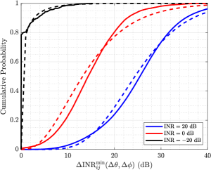
Figure 15: The CDF of $\left\{\Delta\mathsf{INR}_{ij}^{\mathrm{min}}\left(\Delta\theta,\Delta\phi,\mathsf{INR}_{ij}\right):\mathsf{INR}_{ij}\approx\mathsf{INR}\right\}$ for various $\mathsf{INR}$, where $\left(\Delta\theta,\Delta\phi\right)=\left(2^{\circ},2^{\circ}\right)$. Their fitted counterparts are shown as dashed lines.

While fitting the CDFs in Figure 14a directly to normal distributions is useful, it does not capture how the distribution of $\mathsf{INR}_{ij}^{\mathrm{min}}$ varies as a function of $\mathsf{INR}_{ij}$. In other words, it does not provide insight on if high-INR beam pairs are as likely to be within arm’s reach of low INR as low-INR beam pairs are, for instance. To provide more detailed statistics on $\mathsf{INR}_{ij}^{\mathrm{min}}$ based on $\mathsf{INR}_{ij}$, we begin by computing

$$\Delta\mathsf{INR}_{ij}^{\mathrm{min}}\left(\Delta\theta,\Delta\phi,\mathsf{INR}_{ij}\right)=\left[\mathsf{INR}_{ij}\right]_{\mathrm{dB}}-\left[\mathsf{INR}_{ij}^{\mathrm{min}}(\Delta\theta,\Delta\phi)\right]_{\mathrm{dB}}\geq 0$$ (24)

which is the difference (in dB) between the inherent INR offered by the $(i,j)$-th beam pair and the minimum INR of its surrounding $\left(\Delta\theta,\Delta\phi\right)$-neighborhood. We subsequently form the set

$$\mathcal{D}_{\mathrm{min}}\left(\Delta\theta,\Delta\phi,\mathsf{INR}\right)=\left\{\Delta\mathsf{INR}_{ij}^{\mathrm{min}}\left(\Delta\theta,\Delta\phi,\mathsf{INR}_{ij}\right):\mathsf{INR}_{ij}\approx\mathsf{INR}\right\}$$ (25)

which is the set of all $\Delta\mathsf{INR}_{ij}^{\mathrm{min}}(\Delta\theta,\Delta\phi,\mathsf{INR}_{ij})$ values for beam pairs offering an $\mathsf{INR}_{ij}$ of approximately $\mathsf{INR}$. The approximation here is merely used to ensure $\mathcal{D}_{\mathrm{min}}$ has a sufficient number of points in it to successfully fit it, as will become clear. We found that the distribution of $\mathcal{D}_{\mathrm{min}}$ could be well approximated by a Gamma distribution as

$${\mathcal{D}_{\mathrm{min}}\left(\Delta\theta,\Delta\phi,\mathsf{INR}\right)}\overset{\mathrm{fit}}{\sim}\mathrm{Gamma}\left(\alpha_{\mathrm{min}}(\Delta\theta,\Delta\phi,\mathsf{INR}),\beta_{\mathrm{min}}(\Delta\theta,\Delta\phi,\mathsf{INR})\right)$$ (26)

where $\alpha_{\mathrm{min}}(\Delta\theta,\Delta\phi,\mathsf{INR})$ and $\beta_{\mathrm{min}}(\Delta\theta,\Delta\phi,\mathsf{INR})$ are the fitted shape and rate parameters, parameterized by $\mathsf{INR}$ in addition to $\left(\Delta\theta,\Delta\phi\right)$. Alongside the true CDFs of various $\mathcal{D}_{\mathrm{min}}$, we plotted their fitted distributions using dashed lines in Figure 15 for various $\mathsf{INR}$ and a $\left(2^{\circ},2^{\circ}\right)$-neighborhood. This illustrates that extremely low-INR beam pairs tend to see less reduction in INR over their neighborhoods compared to that of high-INR beam pairs. This is somewhat expected but also indicates that low-INR beam pairs are not congregated together but rather spread out throughout our transmit-receive space.

In Table III, we tabulated $(\alpha_{\mathrm{min}},\beta_{\mathrm{min}})$ for $\mathsf{INR}\in\left\{-20,-10,\dots,40\right\}$ dB to provide engineers with $\alpha_{\mathrm{min}}(\Delta\theta,\Delta\phi,\mathsf{INR})$ and $\beta_{\mathrm{min}}(\Delta\theta,\Delta\phi,\mathsf{INR})$ for particular $\mathsf{INR}$ values. To approximate $\alpha_{\mathrm{min}}(\Delta\theta,\Delta\phi,\mathsf{INR})$ and $\beta_{\mathrm{min}}(\Delta\theta,\Delta\phi,\mathsf{INR})$ for any $\mathsf{INR}\in[-20,40]$ dB, weighted interpolation can be used, for instance. It is our hope that this means to realize $\Delta\mathsf{INR}_{ij}^{\mathrm{min}}$ for particular $\mathsf{INR}_{ij}$ is useful for statistical analyses, simulation, and system evaluation. For instance, one may draw $\mathsf{INR}$ from the global distribution (i.e., the CDF in Figure 5) as $\left[\mathsf{INR}\right]_{\mathrm{dB}}\sim\mathcal{N}\left(\mu,\sigma^{2}\right)$ and then use it when referencing Table III to fetch $\alpha_{\mathrm{min}}(\Delta\theta,\Delta\phi,\mathsf{INR})$ and $\beta_{\mathrm{min}}(\Delta\theta,\Delta\phi,\mathsf{INR})$ based on some neighborhood size $\left(\Delta\theta,\Delta\phi\right)$. From there, a realization of $\mathsf{INR}^{\mathrm{min}}(\Delta\theta,\Delta\phi,\mathsf{INR})$ can be drawn as

$$\left[\mathsf{INR}^{\mathrm{min}}(\Delta\theta,\Delta\phi,\mathsf{INR})\right]_{\mathrm{dB}}\sim\left[\mathsf{INR}\right]_{\mathrm{dB}}-\underbrace{\mathrm{Gamma}\left(\alpha_{\mathrm{min}}(\Delta\theta,\Delta\phi,\mathsf{INR}),\beta_{\mathrm{min}}(\Delta\theta,\Delta\phi,\mathsf{INR})\right)}_{\Delta\mathsf{INR}^{\mathrm{min}}\left(\Delta\theta,\Delta\phi,\mathsf{INR}\right)}$$ (27)

which is the minimum INR over the $\left(\Delta\theta,\Delta\phi\right)$-neighborhood surrounding a beam pair offering a nominal INR of $\mathsf{INR}$. Statistical analysis can be conducted using the Gamma distribution, for instance, CDF as follows. When $\Delta\mathsf{INR}^{\mathrm{min}}\left(\Delta\theta,\Delta\phi,\mathsf{INR}\right)$ follows a Gamma distribution with parameters $\alpha_{\mathrm{min}}\left(\Delta\theta,\Delta\phi,\mathsf{INR}\right)$ and $\beta_{\mathrm{min}}\left(\Delta\theta,\Delta\phi,\mathsf{INR}\right)$, the probability that the $\left(\Delta\theta,\Delta\phi\right)$-neighborhood surrounding a random beam pair having an INR of $\mathsf{INR}$ exhibits a minimum INR of $\zeta$ or less is

$$\mathbb{P}\left(\mathsf{INR}^{\mathrm{min}}\leq\zeta;\Delta\theta,\Delta\phi,\mathsf{INR}\right)=\frac{\gamma\left(\alpha_{\mathrm{min}}\left(\Delta\theta,\Delta\phi,\mathsf{INR}\right),\beta_{\mathrm{min}}\left(\Delta\theta,\Delta\phi,\mathsf{INR}\right)\cdot\left[\zeta\right]_{\mathrm{dB}}\right)}{\Gamma(\alpha_{\mathrm{min}}\left(\Delta\theta,\Delta\phi,\mathsf{INR}\right))}$$ (28)

where $\Gamma(\cdot)$ is the Gamma function and $\gamma(\cdot,\cdot)$ is the lower incomplete Gamma function.

IV-C Maximum INR over Various Neighborhoods

As was done for minimum INR over various neighborhoods, we have conducted an analysis and modeling for maximum INR over various neighborhoods. In Figure 16a, we plot the CDF of $\mathsf{INR}_{ij}^{\mathrm{max}}\left(\Delta\theta,\Delta\phi\right)$ of all nearly 6.5 million beam pairs for variably sized neighborhoods. Shown in black is the $\left(0^{\circ},0^{\circ}\right)$-neighborhood, which is simply the CDF of $\mathsf{INR}_{ij}$. Deviating by at most $\left(1^{\circ},1^{\circ}\right)$, the median $\mathsf{INR}_{ij}^{\mathrm{max}}$ sees about a $6$ dB increase from about $20$ dB to $26$ dB. Notice that the lower tail stops around $4$ dB, meaning all nearly 6.5 million beam pairs are within $\left(1^{\circ},1^{\circ}\right)$ of a beam pair offering an INR of $4$ dB or more. Deviating by at most $\left(2^{\circ},2^{\circ}\right)$, the median $\mathsf{INR}_{ij}^{\mathrm{max}}$ increases to $30$ dB and the lower tail stops above $10$ dB. This trend continues with diminishing gains as the neighborhood is widened.

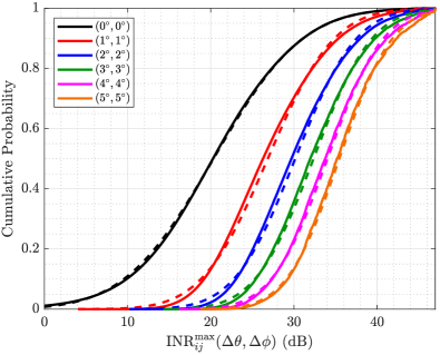
(a) $\mathsf{INR}_{ij}^{\mathrm{max}}(\Delta\theta,\Delta\phi)$.

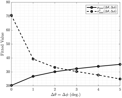
(b) $\mu_{\mathrm{max}}(\Delta\theta,\Delta\phi)$ and $\sigma^{2}_{\mathrm{max}}(\Delta\theta,\Delta\phi)$.

Figure 16: (a) The CDF of $\mathsf{INR}_{ij}^{\mathrm{max}}(\Delta\theta,\Delta\phi)$ for various $(\Delta\theta,\Delta\phi)$. (b) The fitted parameters $\mu_{\mathrm{max}}(\Delta\theta,\Delta\phi)$ and $\sigma^{2}_{\mathrm{max}}(\Delta\theta,\Delta\phi)$ for various $\Delta\theta=\Delta\phi$.

Takeaways.

Before, our analysis of $\mathsf{INR}_{ij}^{\mathrm{min}}$ highlighted that INR levels more attractive for full-duplex operation can be reached by small shifts in transmit and receive steering direction. Figure 16a highlights that small shifts in steering direction can likewise degrade (increase) INR. In fact, even beam pairs with very low INR inherently are highly sensitive, considering a $\left(1^{\circ},1^{\circ}\right)$ shift (at most) can lead to INR levels well above $0$ dB, where full-duplex systems would be overwhelmingly self-interference-limited. As such, small shifts in the transmit and/or receive beams have the potential to drive self-interference to levels unfit for full-duplex. Therefore, if attempting to steer along high-isolation beam pairs to mitigate self-interference, there needs to be fairly high accuracy in doing so, potentially motivating high-resolution phase shifters, for instance.

Like before, we fit a distribution to the CDFs in Figure 16a to offer engineers a statistical tool for $\mathsf{INR}_{ij}^{\mathrm{max}}$. We fit a normal distribution as follows

$$\left\{\left[\mathsf{INR}_{ij}^{\mathrm{max}}(\Delta\theta,\Delta\phi)\right]_{\mathrm{dB}}\ \forall\ i,j\right\}\overset{\mathrm{fit}}{\sim}\mathcal{N}\left(\mu_{\mathrm{max}}(\Delta\theta,\Delta\phi),\sigma^{2}_{\mathrm{max}}(\Delta\theta,\Delta\phi)\right)$$ (29)

where $\mu_{\mathrm{max}}(\Delta\theta,\Delta\phi)$ and $\sigma^{2}_{\mathrm{max}}(\Delta\theta,\Delta\phi)$ are the fitted mean and variance of the normal distribution. The dashed lines in Figure 16a depict each neighborhood’s fitted distribution. Figure 16b shows the resulting fitted $\mu_{\mathrm{max}}\left(\Delta\theta,\Delta\phi\right)$ and $\sigma^{2}_{\mathrm{max}}\left(\Delta\theta,\Delta\phi\right)$ for various $\Delta\theta=\Delta\phi$. Naturally, the mean $\mu_{\mathrm{max}}\left(\Delta\theta,\Delta\phi\right)$ increases with neighborhood size but does so with diminishing gains. The variance $\sigma^{2}_{\mathrm{max}}\left(\Delta\theta,\Delta\phi\right)$ sees a sharp decrease with $\Delta\theta=\Delta\phi=1^{\circ}$ from $0^{\circ}$. This highlights that so many of the nearly 6.5 million beam pairs are within a mere $\left(1^{\circ},1^{\circ}\right)$ of notably higher INR. The variance continues to trend down as the neighborhood widens since high-INR beam pairs can be more reliably reached. In addition to the select neighborhoods in Figure 16a, we have tabulated the fitted parameters $\left(\mu_{\mathrm{max}}\left(\Delta\theta,\Delta\phi\right),\sigma^{2}_{\mathrm{max}}\left(\Delta\theta,\Delta\phi\right)\right)$ for a variety of $\left(\Delta\theta,\Delta\phi\right)$ in Table IV, as was done for $\mathsf{INR}_{ij}^{\mathrm{rng}}$ and $\mathsf{INR}_{ij}^{\mathrm{min}}$. Engineers can use these distributions to conduct a variety of statistical analyses related to $\mathsf{INR}_{ij}^{\mathrm{max}}$ (e.g., worst-case analyses analogous to (23)).

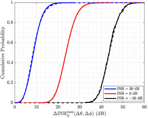
Figure 17: The CDF of $\left\{\Delta\mathsf{INR}_{ij}^{\mathrm{max}}\left(\Delta\theta,\Delta\phi,\mathsf{INR}_{ij}\right):\mathsf{INR}_{ij}\approx\mathsf{INR}\right\}$ for various $\mathsf{INR}$, where $\left(\Delta\theta,\Delta\phi\right)=\left(2^{\circ},2^{\circ}\right)$. Their fitted counterparts are shown as dashed lines. Beam pairs with inherently low INR are typically at a greater risk of large increases in INR caused by small shifts in the transmit and receive beams.

As was done with minimum INR, we conduct a statistical fit of $\mathsf{INR}_{ij}^{\mathrm{max}}$ that depends on $\mathsf{INR}_{ij}$. We define $\Delta\mathsf{INR}_{ij}^{\mathrm{max}}\left(\Delta\theta,\Delta\phi\right)$ as

$$\Delta\mathsf{INR}_{ij}^{\mathrm{max}}\left(\Delta\theta,\Delta\phi,\mathsf{INR}_{ij}\right)=\left[\mathsf{INR}_{ij}^{\mathrm{max}}(\Delta\theta,\Delta\phi)\right]_{\mathrm{dB}}-\left[\mathsf{INR}_{ij}\right]_{\mathrm{dB}}\geq 0$$ (30)

which is the difference (in dB) between the maximum INR within the $\left(\Delta\theta,\Delta\phi\right)$-neighborhood surrounding the $(i,j)$-th transmit-receive beam pair and the INR offered by that beam pair. We form the set

$$\mathcal{D}_{\mathrm{max}}\left(\Delta\theta,\Delta\phi,\mathsf{INR}\right)=\left\{\Delta\mathsf{INR}_{ij}^{\mathrm{max}}\left(\Delta\theta,\Delta\phi,\mathsf{INR}_{ij}\right):\mathsf{INR}_{ij}\approx\mathsf{INR}\right\}$$ (31)

by collecting all $\Delta\mathsf{INR}_{ij}^{\mathrm{max}}\left(\Delta\theta,\Delta\phi,\mathsf{INR}_{ij}\right)$ for beam pairs offering an $\mathsf{INR}_{ij}$ of approximately $\mathsf{INR}$. We again use a Gamma distribution to approximate the distribution of $\mathcal{D}_{\mathrm{max}}$ as

$${\mathcal{D}_{\mathrm{max}}\left(\Delta\theta,\Delta\phi,\mathsf{INR}\right)}\overset{\mathrm{fit}}{\sim}\mathrm{Gamma}\left(\alpha_{\mathrm{max}}(\Delta\theta,\Delta\phi,\mathsf{INR}),\beta_{\mathrm{max}}(\Delta\theta,\Delta\phi,\mathsf{INR})\right)$$ (32)

where $\alpha_{\mathrm{max}}(\Delta\theta,\Delta\phi,\mathsf{INR})$ and $\beta_{\mathrm{max}}(\Delta\theta,\Delta\phi,\mathsf{INR})$ are the fitted shape and rate parameters, parameterized by $\mathsf{INR}$ in addition to $\left(\Delta\theta,\Delta\phi\right)$. We plotted fitted distributions using dashed lines in Figure 17 for various $\mathsf{INR}$ and a $\left(2^{\circ},2^{\circ}\right)$-neighborhood.

In addition, we tabulated $(\alpha_{\mathrm{max}},\beta_{\mathrm{max}})$ for $\mathsf{INR}\in\left\{-20,-10,\dots,40\right\}$ dB to provide engineers with statistical tools. Again, weighted averaging may be used to interpolate between $\mathsf{INR}$ values listed in Table V. Like for minimum INR, $\Delta\mathsf{INR}_{ij}^{\mathrm{max}}$ for particular $\mathsf{INR}_{ij}$ is can be realized using these fitted distributions as follows. One may draw $\mathsf{INR}$ from the global distribution (i.e., the CDF in Figure 5) as $\left[\mathsf{INR}\right]_{\mathrm{dB}}\sim\mathcal{N}\left(\mu,\sigma^{2}\right)$ and then use it when referencing Table V to fetch $\alpha_{\mathrm{max}}(\Delta\theta,\Delta\phi,\mathsf{INR})$ and $\beta_{\mathrm{max}}(\Delta\theta,\Delta\phi,\mathsf{INR})$ based on some neighborhood size $\left(\Delta\theta,\Delta\phi\right)$. A realization of the maximum INR over the $\left(\Delta\theta,\Delta\phi\right)$-neighborhood surrounding a beam pair offering a nominal INR of $\mathsf{INR}$ can be drawn as

$$\left[\mathsf{INR}^{\mathrm{max}}(\Delta\theta,\Delta\phi,\mathsf{INR})\right]_{\mathrm{dB}}\sim\left[\mathsf{INR}\right]_{\mathrm{dB}}+\underbrace{\mathrm{Gamma}\left(\alpha_{\mathrm{max}}(\Delta\theta,\Delta\phi,\mathsf{INR}),\beta_{\mathrm{max}}(\Delta\theta,\Delta\phi,\mathsf{INR})\right)}_{\Delta\mathsf{INR}^{\mathrm{max}}\left(\Delta\theta,\Delta\phi,\mathsf{INR}\right)}$$ (33)

which can facilitate statistical analyses; (28) can be straightforwardly translated from $\mathsf{INR}^{\mathrm{min}}$ to $\mathsf{INR}^{\mathrm{max}}$, for instance. Note that INR range as a function of $\mathsf{INR}$ can be realized using $\mathsf{INR}^{\mathrm{min}}\left(\Delta\theta,\Delta\phi,\mathsf{INR}\right)$ and $\mathsf{INR}^{\mathrm{max}}\left(\Delta\theta,\Delta\phi,\mathsf{INR}\right)$.

V Conclusion

We have collected nearly 6.5 million measurements of multi-panel self-interference at 28 GHz to better understand its spatial and statistical characteristics—providing the most comprehensive examination of such to date. Our measurements illustrate that the degree of self-interference coupled between colocated transmitting and receiving phased arrays tends to be higher when the transmit and receive beams are steered toward one another but small shifts in steering direction (on the order of one degree) can lead to significant changes in such. We have analyzed and statistically modeled this sensitivity, providing engineers with useful insights and statistical tools that can drive system design and evaluation, including those that may use analog and/or digital self-interference cancellation. This measurement campaign sheds light on the efficacy of multi-panel mmWave full-duplex systems, such full-duplex IAB proposed in 3GPP, and motivates strategic beam steering as a potential route to mitigate self-interference without prohibitively compromising beamforming gain. Valuable future work would investigate the impacts of beam shape, array size, environmental reflections, and relative array geometry on self-interference. Future directions capitalizing on this campaign include beam selection for mmWave full-duplex, proposing a practically sound MIMO channel model for mmWave self-interference, and prototyping full-duplex mmWave systems.

Appendix A Tabulated Fitting Results

TABLE I: The fitted parameters $\left(\alpha_{\mathrm{rng}}(\Delta\theta,\Delta\phi),\beta_{\mathrm{rng}}(\Delta\theta,\Delta\phi)\right)$ for various $(\Delta\theta,\Delta\phi)$.

	$0^{\circ}$	$1^{\circ}$	$2^{\circ}$	$3^{\circ}$	$4^{\circ}$	$5^{\circ}$
$0^{\circ}$	—	$(2.74,3.40)$	$(4.42,3.64)$	$(6.73,3.15)$	$(9.50,2.62)$	$(12.50,2.22)$
$1^{\circ}$	$(2.59,3.19)$	$(4.52,4.10)$	$(6.90,3.82)$	$(10.90,2.94)$	$(16.04,2.25)$	$(21.69,1.80)$
$2^{\circ}$	$(4.04,3.48)$	$(6.57,3.85)$	$(10.69,3.11)$	$(17.57,2.21)$	$(25.96,1.64)$	$(34.67,1.30)$
$3^{\circ}$	$(5.80,3.22)$	$(9.63,3.16)$	$(16.31,2.35)$	$(26.67,1.63)$	$(38.06,1.23)$	$(48.77,1.01)$
$4^{\circ}$	$(7.98,2.81)$	$(13.91,2.49)$	$(23.80,1.77)$	$(37.32,1.26)$	$(50.52,0.99)$	$(61.80,0.85)$
$5^{\circ}$	$(10.39,2.44)$	$(18.85,2.00)$	$(31.67,1.42)$	$(47.24,1.05)$	$(61.17,0.86)$	$(72.50,0.76)$

TABLE II: The fitted parameters $\left(\mu_{\mathrm{min}}(\Delta\theta,\Delta\phi),\sigma^{2}_{\mathrm{min}}(\Delta\theta,\Delta\phi)\right)$ for various $(\Delta\theta,\Delta\phi)$.

	$0^{\circ}$	$1^{\circ}$	$2^{\circ}$	$3^{\circ}$	$4^{\circ}$	$5^{\circ}$
$0^{\circ}$	$(20.32,70.69)$	$(15.04,102.75)$	$(10.34,114.62)$	$(6.47,112.94)$	$(3.53,107.37)$	$(1.31,101.93)$
$1^{\circ}$	$(15.58,98.86)$	$(8.32,148.79)$	$(2.30,152.39)$	$(-2.34,135.13)$	$(-5.62,118.00)$	$(-7.98,105.59)$
$2^{\circ}$	$(11.58,109.04)$	$(3.15,153.04)$	$(-3.07,141.96)$	$(-7.56,117.66)$	$(-10.61,99.81)$	$(-12.80,88.34)$
$3^{\circ}$	$(8.23,106.83)$	$(-0.88,137.50)$	$(-6.93,119.30)$	$(-11.07,96.78)$	$(-13.87,82.49)$	$(-15.89,73.80)$
$4^{\circ}$	$(5.50,99.76)$	$(-3.98,118.15)$	$(-9.74,99.32)$	$(-13.57,81.48)$	$(-16.16,70.95)$	$(-18.05,64.68)$
$5^{\circ}$	$(3.39,93.25)$	$(-6.27,103.55)$	$(-11.76,86.70)$	$(-15.37,72.63)$	$(-17.82,64.54)$	$(-19.63,59.62)$

TABLE III: The fitted parameters $\left(\alpha_{\mathrm{min}}\left(\Delta\theta,\Delta\phi,\mathsf{INR}\right),\beta_{\mathrm{min}}\left(\Delta\theta,\Delta\phi,\mathsf{INR}\right)\right)$ for various $\left(\Delta\theta,\Delta\phi,\mathsf{INR}\right)$.

	$\mathsf{INR}$ (dB)
$(\Delta\theta,\Delta\phi)$	$-20$	$-10$	$0$	$10$	$20$	$30$	$40$
$(1^{\circ},1^{\circ})$	$(0.19,1.34)$	$(0.21,11.37)$	$(0.89,10.27)$	$(3.66,4.05)$	$(3.26,3.91)$	$(3.22,2.80)$	$(4.09,1.47)$
$(2^{\circ},2^{\circ})$	$(0.18,4.91)$	$(0.41,13.93)$	$(3.06,4.83)$	$(10.28,2.21)$	$(8.67,2.93)$	$(5.26,4.18)$	$(4.15,4.03)$
$(3^{\circ},3^{\circ})$	$(0.21,9.31)$	$(0.87,10.20)$	$(6.49,2.86)$	$(17.38,1.58)$	$(19.94,1.66)$	$(12.18,2.74)$	$(7.96,3.79)$
$(4^{\circ},4^{\circ})$	$(0.26,12.40)$	$(1.86,6.27)$	$(10.40,2.07)$	$(24.37,1.26)$	$(31.12,1.21)$	$(22.78,1.77)$	$(20.63,1.94)$
$(5^{\circ},5^{\circ})$	$(0.39,11.99)$	$(2.98,4.66)$	$(15.20,1.57)$	$(31.79,1.05)$	$(40.47,1.01)$	$(30.88,1.45)$	$(36.15,1.27)$

TABLE IV: The fitted parameters $\left(\mu_{\mathrm{max}}(\Delta\theta,\Delta\phi),\sigma^{2}_{\mathrm{max}}(\Delta\theta,\Delta\phi)\right)$ for various $(\Delta\theta,\Delta\phi)$.

	$0^{\circ}$	$1^{\circ}$	$2^{\circ}$	$3^{\circ}$	$4^{\circ}$	$5^{\circ}$
$0^{\circ}$	$(20.32,70.69)$	$(24.36,44.95)$	$(26.42,39.02)$	$(27.63,36.81)$	$(28.41,35.64)$	$(29.06,34.66)$
$1^{\circ}$	$(23.84,49.63)$	$(26.85,39.31)$	$(28.64,35.37)$	$(29.71,33.95)$	$(30.41,33.26)$	$(31.00,32.60)$
$2^{\circ}$	$(25.63,45.34)$	$(28.42,37.00)$	$(30.15,33.27)$	$(31.18,31.99)$	$(31.85,31.51)$	$(32.41,31.00)$
$3^{\circ}$	$(26.89,43.38)$	$(29.61,35.48)$	$(31.33,31.57)$	$(32.35,30.31)$	$(33.01,29.93)$	$(33.56,29.52)$
$4^{\circ}$	$(27.89,41.95)$	$(30.61,33.81)$	$(32.35,29.51)$	$(33.38,28.13)$	$(34.02,27.79)$	$(34.57,27.40)$
$5^{\circ}$	$(28.72,40.61)$	$(31.46,32.02)$	$(33.23,27.27)$	$(34.26,25.73)$	$(34.90,25.36)$	$(35.45,24.95)$

TABLE V: The fitted parameters $\left(\alpha_{\mathrm{max}}\left(\Delta\theta,\Delta\phi,\mathsf{INR}\right),\beta_{\mathrm{max}}\left(\Delta\theta,\Delta\phi,\mathsf{INR}\right)\right)$ for various $\left(\Delta\theta,\Delta\phi,\mathsf{INR}\right)$.

	$\mathsf{INR}$ (dB)
$(\Delta\theta,\Delta\phi)$	$-20$	$-10$	$0$	$10$	$20$	$30$	$40$
$(1^{\circ},1^{\circ})$	$(97.36,0.39)$	$(53.69,0.53)$	$(22.22,0.83)$	$(8.27,1.23)$	$(3.94,1.44)$	$(3.65,1.09)$	$(3.73,0.72)$
$(2^{\circ},2^{\circ})$	$(125.30,0.35)$	$(74.38,0.46)$	$(35.07,0.68)$	$(14.26,1.04)$	$(6.18,1.44)$	$(4.83,1.28)$	$(4.76,0.84)$
$(3^{\circ},3^{\circ})$	$(132.69,0.36)$	$(83.02,0.45)$	$(42.63,0.64)$	$(18.35,0.97)$	$(7.76,1.44)$	$(5.40,1.41)$	$(5.37,0.88)$
$(4^{\circ},4^{\circ})$	$(143.23,0.35)$	$(92.33,0.43)$	$(49.46,0.60)$	$(22.61,0.89)$	$(9.53,1.36)$	$(5.96,1.46)$	$(6.10,0.84)$
$(5^{\circ},5^{\circ})$	$(160.40,0.32)$	$(107.86,0.39)$	$(58.95,0.53)$	$(28.38,0.78)$	$(12.12,1.19)$	$(6.53,1.47)$	$(6.94,0.79)$

References

- [1] I. P. Roberts, J. G. Andrews, H. B. Jain, and S. Vishwanath, “Millimeter-wave full duplex radios: New challenges and techniques,” IEEE Wireless Commun., pp. 36–43, Feb. 2021.
- [2] Z. Xiao, P. Xia, and X. Xia, “Full-duplex millimeter-wave communication,” IEEE Wireless Commun., vol. 24, no. 6, pp. 136–143, Dec. 2017.
- [3] X. Liu et al., “Beamforming based full-duplex for millimeter-wave communication,” Sensors, vol. 16, no. 7, p. 1130, Jul. 2016.
- [4] J. Palacios, J. Rodríguez-Fernández, and N. González-Prelcic, “Hybrid precoding and combining for full-duplex millimeter wave communication,” in Proc. IEEE GLOBECOM, Dec. 2019, pp. 1–6.
- [5] K. Satyanarayana, M. El-Hajjar, P. Kuo, A. Mourad, and L. Hanzo, “Hybrid beamforming design for full-duplex millimeter wave communication,” IEEE Trans. Veh. Technol., vol. 68, no. 2, pp. 1394–1404, Feb. 2019.
- [6] Y. Cai, Y. Xu, Q. Shi, B. Champagne, and L. Hanzo, “Robust joint hybrid transceiver design for millimeter wave full-duplex MIMO relay systems,” IEEE Trans. Wireless Commun., vol. 18, no. 2, pp. 1199–1215, Feb. 2019.
- [7] L. Zhu et al., “Millimeter-wave full-duplex UAV relay: Joint positioning, beamforming, and power control,” IEEE JSAC, vol. 38, no. 9, pp. 2057–2073, Sep. 2020.
- [8] I. P. Roberts, J. G. Andrews, and S. Vishwanath, “Hybrid beamforming for millimeter wave full-duplex under limited receive dynamic range,” IEEE Trans. Wireless Commun., vol. 20, no. 12, pp. 7758–7772, Dec. 2021.
- [9] 3GPP, “3GPP TS 38.174: New WID on IAB enhancements,” 2021. [Online]. Available: https://www.3gpp.org/dynareport/38174.htm
- [10] H. Ronkainen, J. Edstam, A. Ericsson, and C. Östberg, “Integrated access and backhaul: A new type of wireless backhaul in 5G,” Frontiers in Communications and Networks, vol. 2, Apr. 2021.
- [11] M. Gupta, I. P. Roberts, and J. G. Andrews, “System-level analysis of full-duplex self-backhauled millimeter wave networks,” Dec. 2021. [Online]. Available: https://arxiv.org/abs/2112.05263
- [12] S. Rajagopal, R. Taori, and S. Abu-Surra, “Self-interference mitigation for in-band mmWave wireless backhaul,” in Proc. IEEE CCNC, Jan. 2014, pp. 551–556.
- [13] Y. Kohda et al., “Single-channel full-duplex mmWave link using phased-array for Ethernet,” in Proc. IEEE CCNC, Jan. 2015, pp. 400–405.
- [14] B. Lee, J. Lim, C. Lim, B. Kim, and J. Seol, “Reflected self-interference channel measurement for mmWave beamformed full-duplex system,” in Proc. IEEE GLOBECOM Wkshp., Dec. 2015, pp. 1–6.
- [15] H. Yang et al., “Interference measurement and analysis of full-duplex wireless system in 60 GHz band,” in Proc. IEEE APCCAS, Oct. 2016, pp. 273–276.
- [16] Y. He, X. Yin, and H. Chen, “Spatiotemporal characterization of self-interference channels for 60-GHz full-duplex communication,” IEEE Antennas Wireless Propag. Lett., vol. 16, pp. 2220–2223, May 2017.
- [17] K. Haneda, J. Järveläinen, A. Karttunen, and J. Putkonen, “Self-interference channel measurements for in-band full-duplex street-level backhaul relays at 70 GHz,” in Proc. IEEE PIMRC, Sep. 2018, pp. 199–204.
- [18] J.-S. Jiang and M. A. Ingram, “Spherical-wave model for short-range MIMO,” IEEE Trans. Commun., vol. 53, no. 9, pp. 1534–1541, Sep. 2005.
- [19] L. Li, K. Josiam, and R. Taori, “Feasibility study on full-duplex wireless millimeter-wave systems,” in Proc. IEEE ICASSP, May 2014, pp. 2769–2773.
- [20] A. Chopra, I. P. Roberts, T. Novlan, and J. G. Andrews, “28 GHz phased array-based self-interference measurements for millimeter wave full-duplex,” in Proc. IEEE WCNC, Apr. 2022, to appear.
- [21] “Anokiwave AWA-0134 5G active antenna innovator kit,” 2021. [Online]. Available: https://www.anokiwave.com/products/awa-0134/index.html
- [22] 3GPP, “3GPP RP-193251: New WID on IAB enhancements,” 2019.
- [23] “Getting Started Guide USRP-2950/2952/2953/2954/2955 - National Instruments,” 2021. [Online]. Available: https://www.ni.com/pdf/manuals/376355c.pdf
- [24] “Millimeter wave products | components | 7GHz to 320GHz,” 2021. [Online]. Available: https://www.miwv.com
- [25] “NRP40SN three path diode power sensor - Rohde & Schwarz,” 2021. [Online]. Available: https://www.rohde-schwarz.com/my/product/nrp40sn-options_63490-160769.html
- [26] “RSC-Z405 RSC step attenuator - Rohde & Schwarz,” 2021. [Online]. Available: https://www.rohde-schwarz.com/us/product/rsc-productstartpage_63493-11395.html
- [27] C. Balanis, Antenna Theory: Analysis and Design. John Wiley & Sons, 2016.