Beyond Adult and COMPAS: Fairness in Multi-Class Prediction

Wael Alghamdi,1∗ Hsiang Hsu,1  Haewon Jeong,1∗ Hao Wang,1
 P. Winston Michalak,1 Shahab Asoodeh,2 and Flavio P. Calmon1
Equal contribution. Correspondence to: Wael Alghamdi (alghamdi@g.harvard.edu) and Flavio P. Calmon (flavio@seas.harvard.edu).
( 1John A. Paulson School of Engineering and Applied Sciences, Harvard University
2Department of Computing and Software, McMaster University
)
Abstract

We consider the problem of producing fair probabilistic classifiers for multi-class classification tasks. We formulate this problem in terms of “projecting” a pre-trained (and potentially unfair) classifier onto the set of models that satisfy target group-fairness requirements. The new, projected model is given by post-processing the outputs of the pre-trained classifier by a multiplicative factor. We provide a parallelizable iterative algorithm for computing the projected classifier and derive both sample complexity and convergence guarantees. Comprehensive numerical comparisons with state-of-the-art benchmarks demonstrate that our approach maintains competitive performance in terms of accuracy-fairness trade-off curves, while achieving favorable runtime on large datasets. We also evaluate our method at scale on an open dataset with multiple classes, multiple intersectional protected groups, and over 1M samples.

1 Introduction

Machine learning (ML) algorithms are increasingly used to automate decisions that have significant social consequences. This trend has led to a surge of research on designing and evaluating fairness interventions that prevent discrimination in ML models. When dealing with group fairness, fairness interventions aim to ensure that a ML model does not discriminate against different groups determined, for example, by race, sex, and/or nationality. Extensive comparisons between discrimination control methods can be found in [8, 32, 54]. As these studies demonstrate, there is still no “best” fairness intervention for ML, with the majority of existing approaches being tailored to either binary classification tasks, binary population groups, or both. Moreover, discrimination control methods are often tested on overused datasets of modest size collected in either the US or Europe (e.g., UCI Adult [47] and COMPAS [7]).

Most fairness interventions111See Related Work and Table 1 for notable exceptions. in ML focus on binary outcomes. In this case, the classification output is either positive or negative, and group-fairness metrics are tailored to binary decisions [35]. While binary classification covers a range of ML tasks of societal importance (e.g., whether to approve a loan, whether to admit a student), there are many cases where the predicted variable is not binary. For example, in education, grading algorithms assign one out of several grades to students. In healthcare, predicted outcomes are frequently not binary (e.g., severity of disease). Even the original COMPAS algorithm—a timeworn case-study in fair ML—assigned a score between 1 to 10 to each pre-trial defendant [7].

We introduce a theoretically-grounded discrimination control method that ensures group fairness in multi-class classification for several, potentially overlapping population groups. We consider group fairness metrics that are natural multi-class extensions of their binary classification counterparts, such as statistical parity [31], equalized odds [35], and error rate imbalance [50, 16]. When restricted to two predicted classes, our method performs competitively against state-of-the-art fairness interventions tailored to binary classification tasks. Our fairness intervention is model-agnostic (i.e., applicable to any model class) and scalable to datasets that are orders of magnitude larger than standard benchmarks found in the fair ML literature.

Our approach is based on an information-theoretic formulation called information projection. We show that this formulation is particularly well-suited for ensuring fairness in probabilistic classifiers with multi-class outputs. Given a probability distribution P𝑃P and a convex set of distributions 𝒫𝒫\mathcal{P}, the goal of information projection is to find the “closest” distribution to P𝑃P in 𝒫𝒫\mathcal{P}. The study of information projection can be traced back to [21], which used KL-divergence to measure “distance” between distributions. Since then, information projection has been extended to other divergence measures, such as f𝑓f-divergences [22] and Rényi divergences [46, 45]. Recently, [3] studied how to project a probabilistic classifier, viewed as a conditional distribution, onto the set of classifiers that satisfy target group-fairness requirements. Remarkably, the projected classifier is obtained by multiplying (i.e., post-processing) the predictions of the original classifier by a factor that depends on the group-fairness constraints.

Prior work on information projection relies on a critical—and limiting—information-theoretic assumption: the underlying probability distributions are known exactly. This is infeasible in practical ML applications, where only a set of training samples from the underlying data distribution is available. We fill this gap by introducing an efficient procedure for computing the projected classifier with finite samples called FairProjection. We establish theoretical guarantees for our algorithm in terms of convergence and sample complexity. Notably, our procedure is parallelizable (e.g., on a GPU). As a result, FairProjection scales to datasets with the number of samples comparable to the population of many US states (>106absentsuperscript106>10^{6} samples). We provide a TensorFlow [1] implementation of our algorithm at [6]. We apply FairProjection to post-process the outputs of probabilistic classifiers in order to ensure group fairness.

We benchmark our post-processing approach against several state-of-the-art fairness interventions selected based on the availability of reproducible code, and qualitatively compare it against many others. Our numerical results are among the most comprehensive comparison of post-processing fairness interventions to date. We present performance results on the HSLS (High School Longitudinal Study, used in [41]), Adult  [47], and COMPAS [7] datasets.

We also evaluate FairProjection on a dataset derived from open and anonymized data from Brazil’s national high school exam—the Exame Nacional do Ensino Médio (ENEM)—with over 1M samples. We made use of this dataset due to the need for large-scale benchmarks for evaluating fairness interventions in multi-class classification tasks. We also answer recent calls [12, 25] for moving away from overused datasets such as Adult [47] and COMPAS [7]. We hope that the ENEM dataset encourages researchers in the field of fair ML to test their methods within broader contexts.222Since (to the best of our knowledge) the ENEM dataset has not been used in fair ML, we provide in Appendix C a datasheet for the ENEM dataset. The data can be found at [37] and code for pre-processing the data can be found at https://github.com/HsiangHsu/Fair-Projection.

In summary, our main contributions are: (i) We introduce a post-processing fairness intervention for multi-class (i.e., non-binary) classification problems that can account for multiple protected groups and is scalable to large datasets; (ii) We derive finite-sample guarantees and convergence-rate results for our post-processing method. Importantly, FairProjection makes information projection practical without requiring exact knowledge of probability distributions; (iii) We demonstrate the favourable performance of our approach through comprehensive benchmarks against state-of-the-art fairness interventions; (iv) We put forth a new large-scale dataset (ENEM) for benchmarking discrimination control methods in multi-class classification tasks; this dataset may encourage researchers in fair ML to evaluate their methods beyond Adult and COMPAS.

Method Feature
Multiclass Multigroup Scores Curve Parallel Rate Metric
Reductions [5] SP, (M)EO
Reject-option [44] SP, (M)EO
EqOdds [35] EO
LevEqOpp [13] FNR
CalEqOdds [50] MEO
FACT [42] SP, (M)EO
Identifying333[39] mention that their method can be applied to multi-class classification, but their reported benchmarks are only for binary classification tasks. [39] superscript\text{{\color[rgb]{0,0.88,0}{\char 33\relax}}}^{\text{{\color[rgb]{0.72,0,0}{\char 35\relax}}}} SP, (M)EO
FST [53, 54] SP, (M)EO
Overlapping [55] SP, (M)EO
Adversarial [57] N/A444[57] is an in-processing method unlike other benchmarks in the table. It does not take a pre-trained classifier as an input. SP, (M)EO
FairProjection (ours) SP, (M)EO
Table 1: Comparison between benchmark methods. Multiclass/multigroup: implementation takes datasets with multiclass/multigroup labels; Scores: processes raw outputs of probabilistic classifiers; Curve: outputs fairness-accuracy tradeoff curves (instead of a single point); Parallel: parallel implementation (e.g., on GPU) is available; Rate: convergence rate or sample complexity guarantee is proved. Metric: applicable fairness metric, with SP\leftrightarrowStatistical Parity, EO\leftrightarrowEqualized Odds, MEO\leftrightarrowMean EO.
Related work.

We summarize key differentiating factors from prior work in Table 1 and provide a more in-depth discussion in Appendix B.4. The fairness interventions that are the most similar to ours are the FairScoreTransformer [53, 54, FST] and the pre-processing method in [39]. The FST and [39] can be viewed as an instantiation of FairProjection restricted to binary classification and cross-entropy (for FST) or KL-divergence (for [39]) as the f𝑓f-divergence of choice. Thus, our approach is a generalization of both methods to multiple f𝑓f-divergences. We also note that, unlike our method, [39] requires retraining a classifier multiple times.

[5] introduced a reductions approach for fair classification. When restricted to binary classification, the benchmarks in Section 5 indicate that the reductions approach consistently achieves the most competitive fairness-accuracy trade-off compared to ours. The approach described here has two key differences from [5]: it is not restricted to binary classification tasks and does not require refitting a classifier several times over the training dataset. These are also key differentiating points from [15], which presented a meta-algorithm for fair classification that accounts for multiple constraints and groups. The reductions approach was later significantly generalized in the GroupFair method by [55] to account for non-overlapping groups and multiple predicted classes. Unlike [55], we do not require retraining classifiers.

Several other recent efforts consider optimizing accuracy under group-fairness constraints. [18] proposed a “proxy-Lagrangian” formulation for incorporating non-differentiable rate constraints which may include group fairness constraints. We avoid non-differentiability issues by considering the probabilities (scores) at the output of the classifier instead of thresholded decisions. [58] introduced a fairness-constrained optimization applicable to margin-based classifiers (our approach can be used on any probabilistic classifier). [48] and [14] characterized fairness-accuracy trade-offs in binary classification tasks when the underlying distributions are known.

Notation.

Boldface Latin letters will always refer to vectors or matrices. The entries of a vector 𝒛𝒛\boldsymbol{z} are denoted by zjsubscript𝑧𝑗z_{j}, and those of a matrix 𝑮𝑮\boldsymbol{G} by Gi,jsubscript𝐺𝑖𝑗G_{i,j}. The all-1 and all-0 vectors are denoted by 𝟏1\mathbf{1} and 𝟎0\mathbf{0}. We set [N]:={1,,N}assigndelimited-[]𝑁1𝑁[N]:=\{1,\cdots,N\} and +[0,)subscript0\mathbb{R}_{+}\triangleq[0,\infty). The probability simplex over [N]delimited-[]𝑁[N] is denoted by 𝚫N{𝒑+N;𝟏T𝒑=1}subscript𝚫𝑁formulae-sequence𝒑superscriptsubscript𝑁superscript1𝑇𝒑1\mathbf{\Delta}_{N}\triangleq\{\boldsymbol{p}\in\mathbb{R}_{+}^{N}~{};~{}\mathbf{1}^{T}\boldsymbol{p}=1\}, and 𝚫N+superscriptsubscript𝚫𝑁\mathbf{\Delta}_{N}^{+} its (relative) interior. If P𝑃P is a Borel probability measure over Nsuperscript𝑁\mathbb{R}^{N}, ZPsimilar-to𝑍𝑃Z\sim P is a random variable, and f:NK:𝑓superscript𝑁superscript𝐾f:\mathbb{R}^{N}\to\mathbb{R}^{K} is Borel, then the expectation of f(Z)𝑓𝑍f(Z) is denoted by 𝔼[f(Z)]=𝔼P[f]=𝔼ZP[f(Z)]𝔼delimited-[]𝑓𝑍subscript𝔼𝑃delimited-[]𝑓subscript𝔼similar-to𝑍𝑃delimited-[]𝑓𝑍\mathbb{E}[f(Z)]=\mathbb{E}_{P}[f]=\mathbb{E}_{Z\sim P}[f(Z)]. We use the standard asymptotic notations O,Θ,𝑂ΘO,\Theta, and ΩΩ\Omega.

2 Problem formulation and preliminaries

Classification tasks.

The essential objects in classification are the input sample space 𝒳𝒳\mathcal{X}, the predicted classes 𝒴𝒴\mathcal{Y}, and the classifiers. We fix two random variables X𝑋X and Y𝑌Y, taking values in sets 𝒳𝒳\mathcal{X} and 𝒴[C]𝒴delimited-[]𝐶\mathcal{Y}\triangleq[C]. Here, (X,Y)𝑋𝑌(X,Y) is a pair comprised of an input sample and corresponding class label randomly drawn from 𝒳×𝒴𝒳𝒴\mathcal{X}\times\mathcal{Y} with distribution PX,Ysubscript𝑃𝑋𝑌P_{X,Y}. A probabilistic classifier is a function 𝒉:𝒳𝚫C:𝒉𝒳subscript𝚫𝐶\boldsymbol{h}:\mathcal{X}\to\mathbf{\Delta}_{C}, where hc(x)subscript𝑐𝑥h_{c}(x) represents the probability of sample x𝒳𝑥𝒳x\in\mathcal{X} falling in class c𝒴𝑐𝒴c\in\mathcal{Y}. Thus, 𝒉𝒉\boldsymbol{h} gives rise to a 𝒴𝒴\mathcal{Y}-valued random variable Y^^𝑌\widehat{Y} via the distribution PY^|X=x(c)hc(x)subscript𝑃conditional^𝑌𝑋𝑥𝑐subscript𝑐𝑥P_{\widehat{Y}|X=x}(c)\triangleq h_{c}(x).

Group-fairness constraints.

Let S𝑆S be a group attribute (e.g., race and/or sex), taking values in 𝒮[A]𝒮delimited-[]𝐴\mathcal{S}\triangleq[A]. We consider multi-class generalization of three commonly used group fairness criteria in Table 2. As observed by existing works [see, e.g., 5, 48, 15, 53, 3], each of these fairness constraints555We remark that our framework can be applied to other fairness constraints, e.g., the ones in [53]. can be written in the vector-inequality form 𝔼PX[𝑮𝒉]𝟎subscript𝔼subscript𝑃𝑋delimited-[]𝑮𝒉0\mathbb{E}_{P_{X}}[\boldsymbol{G}\boldsymbol{h}]\leq\mathbf{0} for a closed-form matrix-valued function 𝑮:𝒳K×C:𝑮𝒳superscript𝐾𝐶\boldsymbol{G}:\mathcal{X}\to\mathbb{R}^{K\times C}. For instance, for statistical parity, the 𝑮𝑮\boldsymbol{G} matrix evaluated at a fixed individual x𝒳𝑥𝒳x\in\mathcal{X} has K=2AC𝐾2𝐴𝐶K=2AC rows indexed by (δ,a,c){0,1}×[A]×[C]𝛿𝑎superscript𝑐01delimited-[]𝐴delimited-[]𝐶(\delta,a,c^{\prime})\in\{0,1\}\times[A]\times[C], where the (δ,a,c)𝛿𝑎superscript𝑐(\delta,a,c^{\prime})-th row is equal to ((1)δPS(a)1c[C]PS|X=x,Y=c(a)hcbase(x)(α+(1)δ))𝒆csuperscript1𝛿subscript𝑃𝑆superscript𝑎1subscript𝑐delimited-[]𝐶subscript𝑃formulae-sequenceconditional𝑆𝑋𝑥𝑌𝑐𝑎superscriptsubscript𝑐base𝑥𝛼superscript1𝛿subscript𝒆superscript𝑐\left((-1)^{\delta}P_{S}(a)^{-1}\sum_{c\in[C]}P_{S|X=x,Y=c}(a)h_{c}^{\mathrm{base}}(x)-(\alpha+(-1)^{\delta})\right)\boldsymbol{e}_{c^{\prime}}, with 𝒆1,,𝒆Csubscript𝒆1subscript𝒆𝐶\boldsymbol{e}_{1},\cdots,\boldsymbol{e}_{C} denoting the standard basis for Csuperscript𝐶\mathbb{R}^{C}. The expressions for the 𝑮𝑮\boldsymbol{G} matrix corresponding to the other fairness metrics are given in Appendix A.7. Note that 𝑮𝑮\boldsymbol{G} depends on PS|X,Ysubscript𝑃conditional𝑆𝑋𝑌P_{S|X,Y}. If the group attribute S𝑆S is part of the input feature X𝑋X, then PS|X,Ysubscript𝑃conditional𝑆𝑋𝑌P_{S|X,Y} is simply replaced with an indicator function. Otherwise, we approximate this conditional distribution by training a probabilistic classifier.

Fairness Criterion Statistical parity Equalized odds Overall accuracy equality
Expression

|PY^|S=a(c)PY^(c)1|αsubscript𝑃conditional^𝑌𝑆𝑎superscript𝑐subscript𝑃^𝑌superscript𝑐1𝛼{\displaystyle\left|\frac{P_{\widehat{Y}|S=a}(c^{\prime})}{P_{\widehat{Y}}(c^{\prime})}-1\right|\leq\alpha}

|PY^|Y=c,S=a(c)PY^|Y=c(c)1|αsubscript𝑃formulae-sequenceconditional^𝑌𝑌𝑐𝑆𝑎superscript𝑐subscript𝑃conditional^𝑌𝑌𝑐superscript𝑐1𝛼{\displaystyle\left|\frac{P_{\widehat{Y}|Y=c,S=a}(c^{\prime})}{P_{\widehat{Y}|Y=c}(c^{\prime})}-1\right|\leq\alpha}

|P(Y^=YS=a)P(Y^=Y)1|α𝑃^𝑌conditional𝑌𝑆𝑎𝑃^𝑌𝑌1𝛼{\displaystyle\left|\frac{P(\widehat{Y}=Y\mid S=a)}{P(\widehat{Y}=Y)}-1\right|\leq\alpha}

Table 2: Standard group fairness criteria; one fixes α>0𝛼0\alpha>0 and iterates over all (a,c,c)[A]×[C]2𝑎𝑐superscript𝑐delimited-[]𝐴superscriptdelimited-[]𝐶2(a,c,c^{\prime})\in[A]\times[C]^{2}.
Goal.

Our goal is to design an efficient post-processing method that takes a pre-trained classifier 𝒉basesuperscript𝒉base\boldsymbol{h}^{\mathrm{base}} that may violate some target group-fairness criteria and finds a fair classifier that has the most similar outputs (i.e., closest utility performance) to that of 𝒉basesuperscript𝒉base\boldsymbol{h}^{\mathrm{base}}.

Fairness through information-projection.

We formulate fair post-processing problem as follows. For a fixed search space 𝚫C𝒳{𝒉:𝒳𝚫C}superscriptsubscript𝚫𝐶𝒳conditional-set𝒉𝒳subscript𝚫𝐶\mathcal{H}\subset\mathbf{\Delta}_{C}^{\mathcal{X}}\triangleq\left\{\boldsymbol{h}:\mathcal{X}\to\mathbf{\Delta}_{C}\right\}, a loss function 𝖾𝗋𝗋:𝚫C𝒳×𝚫C𝒳:𝖾𝗋𝗋superscriptsubscript𝚫𝐶𝒳superscriptsubscript𝚫𝐶𝒳\mathsf{err}:\mathbf{\Delta}_{C}^{\mathcal{X}}\times\mathbf{\Delta}_{C}^{\mathcal{X}}\to\mathbb{R}, and a base classifier 𝒉base𝚫C𝒳superscript𝒉basesuperscriptsubscript𝚫𝐶𝒳\boldsymbol{h}^{\mathrm{base}}\in\mathbf{\Delta}_{C}^{\mathcal{X}}, one seeks to solve:

minimize𝒉𝖾𝗋𝗋(𝒉,𝒉base)subject to𝔼PX[𝑮𝒉]𝟎.𝒉minimize𝖾𝗋𝗋𝒉superscript𝒉basesubject tosubscript𝔼subscript𝑃𝑋delimited-[]𝑮𝒉0\displaystyle\underset{\boldsymbol{h}\in\mathcal{H}}{\text{minimize}}\ \mathsf{err}\left(\boldsymbol{h},\boldsymbol{h}^{\mathrm{base}}\right)\quad\text{subject to}\ \mathbb{E}_{P_{X}}\left[\boldsymbol{G}\boldsymbol{h}\right]\leq\mathbf{0}. (1)

The function 𝖾𝗋𝗋𝖾𝗋𝗋\mathsf{err} quantifies the “closeness” between the scores given by 𝒉𝒉\boldsymbol{h} and 𝒉basesuperscript𝒉base\boldsymbol{h}^{\mathrm{base}} and we choose f𝑓f-divergence to measure this:

𝖾𝗋𝗋(𝒉,𝒉base)=Df(𝒉𝒉basePX)𝔼PX[c[C]hcbase(X)f(hc(X)hcbase(X))]f(1),𝖾𝗋𝗋𝒉superscript𝒉basesubscript𝐷𝑓𝒉delimited-‖∣superscript𝒉basesubscript𝑃𝑋subscript𝔼subscript𝑃𝑋delimited-[]subscript𝑐delimited-[]𝐶subscriptsuperscriptbase𝑐𝑋𝑓subscript𝑐𝑋superscriptsubscript𝑐base𝑋𝑓1\displaystyle\mathsf{err}\left(\boldsymbol{h},\boldsymbol{h}^{\mathrm{base}}\right)=D_{f}(\boldsymbol{h}\|\boldsymbol{h}^{\mathrm{base}}\mid P_{X})\triangleq\mathbb{E}_{P_{X}}\left[\sum_{c\in[C]}h^{\mathrm{base}}_{c}(X)f\left(\frac{h_{c}(X)}{h_{c}^{\mathrm{base}}(X)}\right)\right]-f(1), (2)

where f𝑓f is a convex function over (0,)0(0,\infty). By varying different choices of f𝑓f, we can obtain e.g., cross-entropy (CE, f(t)=logt𝑓𝑡𝑡f(t)=-\log t) and KL-divergence (f(t)=tlogt𝑓𝑡𝑡𝑡f(t)=t\log t). For a chosen f𝑓f-divergence, the optimization problem (1) becomes a generalization of information projection [21].

Preliminaries on information-projection.

In a recent work [3], an optimal solution for the information projection formulation (1) was theoretically characterized. We briefly describe this result next. Let666Here, 𝒞(𝒳,𝚫C)𝒞𝒳subscript𝚫𝐶\mathcal{C}(\mathcal{X},\mathbf{\Delta}_{C}) denotes the complete metric space of continuous functions from 𝒳𝒳\mathcal{X} to 𝚫Csubscript𝚫𝐶\mathbf{\Delta}_{C}, equipped with the sup-norm, i.e., 𝒉supx𝒳𝒉(x)1norm𝒉subscriptsupremum𝑥𝒳subscriptnorm𝒉𝑥1\|\boldsymbol{h}\|\triangleq\sup_{x\in\mathcal{X}}\|\boldsymbol{h}(x)\|_{1}. {𝒉𝒞(𝒳,𝚫C);infc,xhc(x)>0}formulae-sequence𝒉𝒞𝒳subscript𝚫𝐶subscriptinfimum𝑐𝑥subscript𝑐𝑥0\mathcal{H}\triangleq\left\{\boldsymbol{h}\in\mathcal{C}(\mathcal{X},\mathbf{\Delta}_{C})~{};~{}\inf_{c,x}h_{c}(x)>0\right\} and we introduce the following definition and assumption.

Definition 1.

For 𝒑𝚫C𝒑subscript𝚫𝐶\boldsymbol{p}\in\mathbf{\Delta}_{C}, let Dfconj(,𝒑)superscriptsubscript𝐷𝑓conj𝒑D_{f}^{\mathrm{conj}}(\,\cdot\,,\boldsymbol{p}) denote the convex conjugate of Df(𝒑)D_{f}(\,\cdot\,\|\,\boldsymbol{p}):

Dfconj(𝒗,𝒑)sup𝒒𝚫C𝒗T𝒒Df(𝒒𝒑).superscriptsubscript𝐷𝑓conj𝒗𝒑subscriptsupremum𝒒subscript𝚫𝐶superscript𝒗𝑇𝒒subscript𝐷𝑓conditional𝒒𝒑D_{f}^{\mathrm{conj}}(\boldsymbol{v},\boldsymbol{p})\triangleq\sup_{\boldsymbol{q}\in\mathbf{\Delta}_{C}}\boldsymbol{v}^{T}\boldsymbol{q}-D_{f}(\boldsymbol{q}\,\|\,\boldsymbol{p}). (3)
Assumption 1.

Assume that: (i) f𝒞2()𝑓superscript𝒞2f\in\mathcal{C}^{2}(\mathbb{R}), f(1)=0,𝑓10f(1)=0, f(0+)=superscript𝑓superscript0f^{\prime}(0^{+})=-\infty, and f′′(t)>0superscript𝑓′′𝑡0f^{\prime\prime}(t)>0 for all t>0𝑡0t>0; (ii) each Gk,csubscript𝐺𝑘𝑐G_{k,c} is bounded, differentiable, and has bounded gradient; (iii) 𝒉basesuperscript𝒉base\boldsymbol{h}^{\mathrm{base}}\in\mathcal{H}, and each hcbasesubscriptsuperscriptbase𝑐h^{\mathrm{base}}_{c} has bounded partial derivatives; and (iv) there is an 𝒉𝒉\boldsymbol{h}\in\mathcal{H} such that 𝔼PX[𝑮𝒉]<𝟎subscript𝔼subscript𝑃𝑋delimited-[]𝑮𝒉0\mathbb{E}_{P_{X}}[\boldsymbol{G}\boldsymbol{h}]<\mathbf{0}.

Now, the solution for (1) can be obtained by a simple “tilting” of the base classifier’s output, as stated in the next theorem.

Theorem 1 ([3]).

If f,𝐡base,𝑓superscript𝐡basef,\boldsymbol{h}^{\mathrm{base}}, and 𝐆𝐆\boldsymbol{G} satisfy Assumption 1, and 𝒳=d𝒳superscript𝑑\mathcal{X}=\mathbb{R}^{d}, then there is a unique solution 𝐡optsuperscript𝐡opt\boldsymbol{h}^{\mathrm{opt}} for the optimization problem (1) for the f𝑓f-divergence objective (2)italic-(2italic-)\eqref{eq:f-divergence}. Furthermore, 𝐡optsuperscript𝐡opt\boldsymbol{h}^{\mathrm{opt}} is given by the tilt

hcopt(x)=hcbase(x)ϕ(vc(x;𝝀)+γ(x;𝝀)),(x,c)𝒳×[C],formulae-sequencesuperscriptsubscript𝑐opt𝑥superscriptsubscript𝑐base𝑥italic-ϕsubscript𝑣𝑐𝑥superscript𝝀𝛾𝑥superscript𝝀𝑥𝑐𝒳delimited-[]𝐶h_{c}^{\mathrm{opt}}(x)=h_{c}^{\mathrm{base}}(x)\cdot\phi\left(v_{c}(x;\boldsymbol{\lambda}^{\star})+\gamma(x;\boldsymbol{\lambda}^{\star})\right),\qquad(x,c)\in\mathcal{X}\times[C], (4)

where: (i) the function ϕitalic-ϕ\phi denotes the inverse of fsuperscript𝑓f^{\prime}; (ii) the function 𝐯:𝒳×KC:𝐯𝒳superscript𝐾superscript𝐶\boldsymbol{v}:\mathcal{X}\times\mathbb{R}^{K}\to\mathbb{R}^{C} is defined by 𝐯(x;𝛌)𝐆(x)T𝛌𝐯𝑥𝛌𝐆superscript𝑥𝑇𝛌\boldsymbol{v}(x;\boldsymbol{\lambda})\triangleq-\boldsymbol{G}(x)^{T}\boldsymbol{\lambda}; (iii) the function γ:𝒳×K:𝛾𝒳superscript𝐾\gamma:\mathcal{X}\times\mathbb{R}^{K}\to\mathbb{R} is characterized by the equation 𝔼c𝐡base(x)[ϕ(vc(x;𝛌)+γ(x;𝛌))]=1subscript𝔼similar-to𝑐superscript𝐡base𝑥delimited-[]italic-ϕsubscript𝑣𝑐𝑥𝛌𝛾𝑥𝛌1\mathbb{E}_{c\sim\boldsymbol{h}^{\mathrm{base}}(x)}\left[\phi\left(v_{c}(x;\boldsymbol{\lambda})+\gamma(x;\boldsymbol{\lambda})\right)\right]=1; and (iv) 𝛌Ksuperscript𝛌superscript𝐾\boldsymbol{\lambda}^{\star}\in\mathbb{R}^{K} is any solution to the convex problem

Dmin𝝀+K𝔼[Dfconj(𝒗(X;𝝀),𝒉base(X))].superscript𝐷subscript𝝀superscriptsubscript𝐾𝔼delimited-[]superscriptsubscript𝐷𝑓conj𝒗𝑋𝝀superscript𝒉base𝑋D^{\star}\triangleq\min_{\boldsymbol{\lambda}\in\mathbb{R}_{+}^{K}}~{}\mathbb{E}\left[D_{f}^{\mathrm{conj}}\left(\boldsymbol{v}(X;\boldsymbol{\lambda}),\boldsymbol{h}^{\mathrm{base}}(X)\right)\right]. (5)

If the underlying data distribution is known, Theorem 1 yields an expression for the projected classifier as a post-processing of the base classifier. However, in practice, we do not know the underlying distribution and have to approximate it from a finite number of i.i.d. samples. In Section 3, we first describe how we approximate the solution given in Theorem 1 with finite samples. We then propose a parallelizable algorithm to solve the approximation in Section 4.

3 A finite-sample approximation of information projection

In practice, PXsubscript𝑃𝑋P_{X} is unknown and only data points 𝕏{Xi}i[N]𝒳𝕏subscriptsubscript𝑋𝑖𝑖delimited-[]𝑁𝒳\mathbb{X}\triangleq\{X_{i}\}_{i\in[N]}\subset\mathcal{X}, drawn from PXsubscript𝑃𝑋P_{X}, are available. Thus, we propose the following fairness optimization problem. We search for a (multi-class) classifier 𝒉:𝕏𝚫C:𝒉𝕏subscript𝚫𝐶\boldsymbol{h}:\mathbb{X}\to\mathbf{\Delta}_{C} that solves the following:

minimize𝒉:𝕏𝚫C𝒂:𝕏C,𝒃K:𝒉𝕏subscript𝚫𝐶:𝒂formulae-sequence𝕏superscript𝐶𝒃superscript𝐾minimize\displaystyle\underset{\begin{subarray}{c}\boldsymbol{h}:\mathbb{X}\to\mathbf{\Delta}_{C}\\ \boldsymbol{a}:\mathbb{X}\to\mathbb{R}^{C},\boldsymbol{b}\in\mathbb{R}^{K}\end{subarray}}{\textup{minimize}} Df(𝒉𝒉baseP^X)+τ1(𝔼XP^X[𝒂(X)22]+𝒃22)subscript𝐷𝑓𝒉delimited-‖∣superscript𝒉basesubscript^𝑃𝑋subscript𝜏1subscript𝔼similar-to𝑋subscript^𝑃𝑋delimited-[]superscriptsubscriptnorm𝒂𝑋22superscriptsubscriptnorm𝒃22\displaystyle D_{f}\left(\boldsymbol{h}\,\|\,\boldsymbol{h}^{\mathrm{base}}\mid\widehat{P}_{X}\right)+\tau_{1}\cdot\left(\mathbb{E}_{X\sim\widehat{P}_{X}}\left[\|\boldsymbol{a}(X)\|_{2}^{2}\right]+\|\boldsymbol{b}\|_{2}^{2}\right) (6)
subject to 𝔼P^X[𝑮(𝒉+τ2𝒂)]τ2𝒃,subscript𝔼subscript^𝑃𝑋delimited-[]𝑮𝒉subscript𝜏2𝒂subscript𝜏2𝒃\displaystyle\mathbb{E}_{\widehat{P}_{X}}\left[\boldsymbol{G}\cdot(\boldsymbol{h}+\tau_{2}\boldsymbol{a})\right]\leq\tau_{2}\boldsymbol{b},

with P^Xsubscript^𝑃𝑋\widehat{P}_{X} being the empirical measure (e.g., obtained from a dataset), and τ1,τ2>0subscript𝜏1subscript𝜏20\tau_{1},\tau_{2}>0 prescribed constants. The terms 𝒂𝒂\boldsymbol{a} and 𝒃𝒃\boldsymbol{b} are added to circumvent infeasibility issues and aid convergence of our numerical procedure. We show in the following theorem that there is a unique solution for (6), and that it is given by a tilt (i.e., multiplicative factor) of 𝒉basesuperscript𝒉base\boldsymbol{h}^{\mathrm{base}}. The tilting parameter is the solution of a finite-dimensional strongly convex optimization problem.

Theorem 2.

Suppose Assumption 1 holds, and set ζτ22/(2τ1)𝜁superscriptsubscript𝜏222subscript𝜏1\zeta\triangleq\tau_{2}^{2}/(2\tau_{1}). There exists a unique solution 𝐡opt,Nsuperscript𝐡opt𝑁\boldsymbol{h}^{\mathrm{opt},N} to (6), and it is given by the formula

hcopt,N(x)=hcbase(x)ϕ(vc(x;𝝀ζ,N)+γ(x;𝝀ζ,N)),(x,c)𝕏×[C],formulae-sequencesuperscriptsubscript𝑐opt𝑁𝑥superscriptsubscript𝑐base𝑥italic-ϕsubscript𝑣𝑐𝑥subscriptsuperscript𝝀𝜁𝑁𝛾𝑥subscriptsuperscript𝝀𝜁𝑁𝑥𝑐𝕏delimited-[]𝐶h_{c}^{\mathrm{opt},N}(x)=h_{c}^{\mathrm{base}}(x)\cdot\phi\left(v_{c}(x;\boldsymbol{\lambda}^{\star}_{\zeta,N})+\gamma(x;\boldsymbol{\lambda}^{\star}_{\zeta,N})\right),\quad(x,c)\in\mathbb{X}\times[C], (7)

with 𝐯,ϕ,γ𝐯italic-ϕ𝛾\boldsymbol{v},\phi,\gamma as in Theorem 1, and 𝛌ζ,NKsuperscriptsubscript𝛌𝜁𝑁superscript𝐾\boldsymbol{\lambda}_{\zeta,N}^{\star}\in\mathbb{R}^{K} is the unique solution to the strongly convex problem

Dζ,Nmin𝝀+K𝔼P^X[Dfconj(𝒗(X;𝝀),𝒉base(X))]+ζ2𝓖NT𝝀22superscriptsubscript𝐷𝜁𝑁subscript𝝀superscriptsubscript𝐾subscript𝔼subscript^𝑃𝑋delimited-[]superscriptsubscript𝐷𝑓conj𝒗𝑋𝝀superscript𝒉base𝑋𝜁2superscriptsubscriptnormsuperscriptsubscript𝓖𝑁𝑇𝝀22D_{\zeta,N}^{\star}\triangleq\min_{\boldsymbol{\lambda}\in\mathbb{R}_{+}^{K}}~{}\mathbb{E}_{\widehat{P}_{X}}\left[D_{f}^{\mathrm{conj}}\left(\boldsymbol{v}(X;\boldsymbol{\lambda}),\boldsymbol{h}^{\mathrm{base}}(X)\right)\right]+\frac{\zeta}{2}\left\|\boldsymbol{\mathcal{G}}_{N}^{T}\boldsymbol{\lambda}\right\|_{2}^{2} (8)

where 𝓖N(𝐆(X1)/N,,𝐆(XN)/N,𝐈K)K×(NC+K)subscript𝓖𝑁𝐆subscript𝑋1𝑁𝐆subscript𝑋𝑁𝑁subscript𝐈𝐾superscript𝐾𝑁𝐶𝐾\boldsymbol{\mathcal{G}}_{N}\triangleq\left(\boldsymbol{G}(X_{1})/\sqrt{N},\cdots,\boldsymbol{G}(X_{N})/\sqrt{N},\boldsymbol{I}_{K}\right)\in\mathbb{R}^{K\times(NC+K)}.

Proof.

See Appendix A.1. ∎

Theorem 2 shows that: strong duality holds between the primal (6) and (the negative of) the dual (8); there is a unique classifier 𝒉opt,Nsuperscript𝒉opt𝑁\boldsymbol{h}^{\mathrm{opt},N} minimizing our fairness formulation (6); there is a unique solution 𝝀ζ,Nsuperscriptsubscript𝝀𝜁𝑁\boldsymbol{\lambda}_{\zeta,N}^{\star} to the dual (5); and there is an explicit functional form of 𝒉opt,Nsuperscript𝒉opt𝑁\boldsymbol{h}^{\mathrm{opt},N} in terms of 𝝀ζ,Nsuperscriptsubscript𝝀𝜁𝑁\boldsymbol{\lambda}_{\zeta,N}^{\star} in (7).

The key distinctions between our formulation and Theorem 1 are that we use the empirical measure P^Xsubscript^𝑃𝑋\widehat{P}_{X} (e.g., produced using a dataset with i.i.d. samples), we have a strongly convex dual problem in (8) (in contrast to the convex program in (5)), and we prove strong duality in Theorem 2 (whereas an analogous strong duality is absent from the results of [3]). Hence, Theorem 2 yields a practical two-step procedure for solving the functional optimization in equation (6): (i) compute the dual variables by solving the strongly convex optimization in (8); (ii) tilt the base classifier by using the dual variables according to (7). This process is applied on real-world datasets using FairProjection (see Algorithm 1) in the next section.

The results of Theorem 2 are tightly related to those in information projection shown in Theorem 1, which corresponds to the case τ1=τ2=ζ=0subscript𝜏1subscript𝜏2𝜁0\tau_{1}=\tau_{2}=\zeta=0 and PXsubscript𝑃𝑋P_{X} in place of P^Xsubscript^𝑃𝑋\widehat{P}_{X}. We show in Theorem 4 in the next section that the choice ζN1/2proportional-to𝜁superscript𝑁12\zeta\propto N^{-1/2} yields a sense in which our numerically obtained (from FairProjection) tilting parameters 𝝀𝝀\boldsymbol{\lambda} work well for the population problem (5).

Remark 1.

In practice, Assumption 1 is not a limiting factor for Theorem 2 and FairProjection. This is because: we are considering here a finite-set domain so continuity is automatic; we can perturb 𝒉basesuperscript𝒉base\boldsymbol{h}^{\mathrm{base}} by negligible noise to push it away from the simplex boundary; and the uniform classifier is strictly feasible. Nevertheless, Assumption 1 simplifies the derivation of our theoretical results.

4 Fair projection and theoretical guarantees

We introduce a parallelizable algorithm, FairProjection, that solves (6) using N𝑁N i.i.d. data points. We prove that its utility converges to Dsuperscript𝐷D^{\star} (see (5)) in the population limit and establish both sample-complexity and convergence rate guarantees. Applying FairProjection to the group-fairness intervention problem in (1) yields the optimal parameters in (7) for post-processing (i.e., tilting) the output of a multi-class classifier in order to satisfy target fairness constraints.

Algorithm 1 : FairProjection for solving (8).
  Input: divergence f𝑓f, predictions {𝒑i𝒉base(Xi)}i[N]subscriptsubscript𝒑𝑖superscript𝒉basesubscript𝑋𝑖𝑖delimited-[]𝑁\{\boldsymbol{p}_{i}\triangleq\boldsymbol{h}^{\mathrm{base}}(X_{i})\}_{i\in[N]}, constraints {𝑮i𝑮(Xi)}i[N]subscriptsubscript𝑮𝑖𝑮subscript𝑋𝑖𝑖delimited-[]𝑁\{\boldsymbol{G}_{i}\triangleq\boldsymbol{G}(X_{i})\}_{i\in[N]}, regularizer ζ𝜁\zeta, ADMM penalty ρ𝜌\rho, and initializers 𝝀𝝀\boldsymbol{\lambda} and (𝒘i)i[N]subscriptsubscript𝒘𝑖𝑖delimited-[]𝑁(\boldsymbol{w}_{i})_{i\in[N]}.
  Output: hcopt,N(x)hcbase(x)ϕ(γ(x;𝝀)+vc(x;𝝀))superscriptsubscript𝑐opt𝑁𝑥superscriptsubscript𝑐base𝑥italic-ϕ𝛾𝑥𝝀subscript𝑣𝑐𝑥𝝀h_{c}^{\mathrm{opt},N}(x)\triangleq h_{c}^{\mathrm{base}}(x)\cdot\phi(\gamma(x;\boldsymbol{\lambda})+v_{c}(x;\boldsymbol{\lambda})).
  𝑸ζ2𝑰+ρ2Ni[N]𝑮i𝑮iT𝑸𝜁2𝑰𝜌2𝑁subscript𝑖delimited-[]𝑁subscript𝑮𝑖superscriptsubscript𝑮𝑖𝑇\boldsymbol{Q}\leftarrow\frac{\zeta}{2}\boldsymbol{I}+\frac{\rho}{2N}\sum_{i\in[N]}\boldsymbol{G}_{i}\boldsymbol{G}_{i}^{T}
  for t=1,2,,t𝑡12superscript𝑡t=1,2,\cdots,t^{\prime} do
     𝒂i𝒘i+ρ𝑮iT𝝀i[N]subscript𝒂𝑖subscript𝒘𝑖𝜌superscriptsubscript𝑮𝑖𝑇𝝀𝑖delimited-[]𝑁\boldsymbol{a}_{i}\leftarrow\boldsymbol{w}_{i}+\rho\boldsymbol{G}_{i}^{T}\boldsymbol{\lambda}\lx@algorithmic@hfill~{}i\in[N]
     𝒗iargmin𝒗CDfconj(𝒗,𝒑i)+ρ+ζ2𝒗22+𝒂iT𝒗i[N]subscript𝒗𝑖𝒗superscript𝐶argminsuperscriptsubscript𝐷𝑓conj𝒗subscript𝒑𝑖𝜌𝜁2superscriptsubscriptnorm𝒗22superscriptsubscript𝒂𝑖𝑇𝒗𝑖delimited-[]𝑁\boldsymbol{v}_{i}\leftarrow\underset{\boldsymbol{v}\in\mathbb{R}^{C}}{\mathrm{argmin}}~{}D_{f}^{\mathrm{conj}}(\boldsymbol{v},\boldsymbol{p}_{i})+\frac{\rho+\zeta}{2}\|\boldsymbol{v}\|_{2}^{2}+\boldsymbol{a}_{i}^{T}\boldsymbol{v}\lx@algorithmic@hfill~{}i\in[N]
     𝒒1Ni[N]𝑮i(𝒘i+𝒗i)𝒒1𝑁subscript𝑖delimited-[]𝑁subscript𝑮𝑖subscript𝒘𝑖subscript𝒗𝑖\boldsymbol{q}\leftarrow\frac{1}{N}{\displaystyle\sum_{i\in[N]}}\boldsymbol{G}_{i}\cdot\left(\boldsymbol{w}_{i}+\boldsymbol{v}_{i}\right)
     𝝀argmin+KT𝑸+𝒒T𝝀bold-ℓsuperscriptsubscript𝐾argminsuperscriptbold-ℓ𝑇𝑸bold-ℓsuperscript𝒒𝑇bold-ℓ\boldsymbol{\lambda}\leftarrow\underset{\boldsymbol{\ell}\in\mathbb{R}_{+}^{K}}{\mathrm{argmin}}~{}\boldsymbol{\ell}^{T}\boldsymbol{Q}\boldsymbol{\ell}+\boldsymbol{q}^{T}\boldsymbol{\ell}
     𝒘i𝒘i+ρ(𝒗i+𝑮iT𝝀)i[N]subscript𝒘𝑖subscript𝒘𝑖𝜌subscript𝒗𝑖superscriptsubscript𝑮𝑖𝑇𝝀𝑖delimited-[]𝑁\boldsymbol{w}_{i}\leftarrow\boldsymbol{w}_{i}+\rho\cdot\left(\boldsymbol{v}_{i}+\boldsymbol{G}_{i}^{T}\boldsymbol{\lambda}\right)\lx@algorithmic@hfill i\in[N]
  end for

The FairProjection algorithm uses ADMM [11] to solve the convex program in (8). Recall that it suffices to optimize (8) for computing (6) as proved in Theorem 2. Algorithm 1 presents the steps of FairProjection, and its detailed derivation is given in Appendix A.2. A salient feature of FairProjection is its parallelizability. Each step that is done for i𝑖i varying over [N]delimited-[]𝑁[N] can be executed for each i𝑖i separately and in parallel. In particular, this applies to the most computationally intensive step, the 𝒗isubscript𝒗𝑖\boldsymbol{v}_{i}-update step. We discuss next how the 𝒗isubscript𝒗𝑖\boldsymbol{v}_{i}-update step is carried out.

Inner iterations.

One approach to carry out the inner iteration in Algorithm 1 that updates 𝒗isubscript𝒗𝑖\boldsymbol{v}_{i} is to study the vanishing of the gradient of 𝒗Dfconj(𝒗,𝒑i)+ξ𝒗22+𝒂iT𝒗maps-to𝒗superscriptsubscript𝐷𝑓conj𝒗subscript𝒑𝑖𝜉superscriptsubscriptnorm𝒗22superscriptsubscript𝒂𝑖𝑇𝒗\boldsymbol{v}\mapsto D_{f}^{\mathrm{conj}}(\boldsymbol{v},\boldsymbol{p}_{i})+\xi\|\boldsymbol{v}\|_{2}^{2}+\boldsymbol{a}_{i}^{T}\boldsymbol{v} (where ξ=(ρ+ζ)/2𝜉𝜌𝜁2\xi=(\rho+\zeta)/2 and 𝒂iCsubscript𝒂𝑖superscript𝐶\boldsymbol{a}_{i}\in\mathbb{R}^{C} is some vector). In the KL-divergence case, D𝖪𝖫conjsuperscriptsubscript𝐷𝖪𝖫conjD_{\mathsf{KL}}^{\mathrm{conj}} is given by a log-sum-exp function, so its gradient is given by a softmax function, and equating the gradient to zero becomes a fixed-point equation. We give an iterative routine to solve this fixed point equation in Appendix A.3.1, whose proof of convergence is aided by our proof that the softmax function is 1212\frac{1}{2}-Lipschitz in Appendix A.4. Beyond the KL-divergence case, setting the gradient to zero does not seem to be an analytically tractable problem. Nevertheless, we may reduce the vector minimization in the 𝒗isubscript𝒗𝑖\boldsymbol{v}_{i}-step to a tractable 111-dimensional root-finding problem, as the following result aids in showing.

Lemma 1.

For 𝐩𝚫C+𝐩superscriptsubscript𝚫𝐶\boldsymbol{p}\in\mathbf{\Delta}_{C}^{+}, 𝐚C𝐚superscript𝐶\boldsymbol{a}\in\mathbb{R}^{C}, and ξ>0𝜉0\xi>0, if f𝑓f satisfies Assumption 1, we have that

min𝒗CDfconj(𝒗,𝒑)+ξ𝒗22+𝒂T𝒗=supθθ+c[C]minqc0pcf(qcpc)+(ac+qc)24ξ+θqc.subscript𝒗superscript𝐶superscriptsubscript𝐷𝑓conj𝒗𝒑𝜉superscriptsubscriptnorm𝒗22superscript𝒂𝑇𝒗subscriptsupremum𝜃𝜃subscript𝑐delimited-[]𝐶subscriptsubscript𝑞𝑐0subscript𝑝𝑐𝑓subscript𝑞𝑐subscript𝑝𝑐superscriptsubscript𝑎𝑐subscript𝑞𝑐24𝜉𝜃subscript𝑞𝑐\displaystyle\min_{\boldsymbol{v}\in\mathbb{R}^{C}}D_{f}^{\mathrm{conj}}(\boldsymbol{v},\boldsymbol{p})+\xi\|\boldsymbol{v}\|_{2}^{2}+\boldsymbol{a}^{T}\boldsymbol{v}=-\sup_{\theta\in\mathbb{R}}-\theta+\sum_{c\in[C]}\min_{q_{c}\geq 0}~{}p_{c}f\left(\frac{q_{c}}{p_{c}}\right)+\frac{(a_{c}+q_{c})^{2}}{4\xi}+\theta q_{c}. (9)
Proof.

See Appendix A.3.2. ∎

We note that the 𝒗isubscript𝒗𝑖\boldsymbol{v}_{i}-update steps for both KL and CE (provided in detail in Appendix A.3.3) give, as a byproduct, the implicitly defined function γ(x;𝝀)𝛾𝑥𝝀\gamma(x;\boldsymbol{\lambda}) (see the statements of Theorems 12).

Convergence guarantees.

Our proposed algorithm, FairProjection, enjoys the following convergence guarantees. First, the output after the t𝑡t-th iteration 𝝀ζ,N(t)superscriptsubscript𝝀𝜁𝑁𝑡\boldsymbol{\lambda}_{\zeta,N}^{(t)} converges exponentially fast to 𝝀ζ,Nsuperscriptsubscript𝝀𝜁𝑁\boldsymbol{\lambda}_{\zeta,N}^{\star} (see (8)).

Theorem 3.

If Assumption 1 holds, the FairProjection algorithm for KL-divergence converges in t=O(logN)superscript𝑡𝑂𝑁t^{\prime}=O(\log N) steps, and runs in time O(NlogN)𝑂𝑁𝑁O(N\log N), to the unique solution 𝛌ζ,Nsuperscriptsubscript𝛌𝜁𝑁\boldsymbol{\lambda}_{\zeta,N}^{\star} of (8). Further, if 𝛌ζ,N(t)superscriptsubscript𝛌𝜁𝑁𝑡\boldsymbol{\lambda}_{\zeta,N}^{(t)} and 𝐡(t)superscript𝐡𝑡\boldsymbol{h}^{(t)} are the t𝑡t-th iteration outputs of FairProjection, then 𝛌ζ,N(t)𝛌ζ,N2=O(et)subscriptnormsuperscriptsubscript𝛌𝜁𝑁𝑡superscriptsubscript𝛌𝜁𝑁2𝑂superscript𝑒𝑡\|\boldsymbol{\lambda}_{\zeta,N}^{(t)}-\boldsymbol{\lambda}_{\zeta,N}^{\star}\|_{2}=O(e^{-t}) and 𝐡(t)(x)=𝐡opt,N(x)(1+O(et))superscript𝐡𝑡𝑥superscript𝐡opt𝑁𝑥1𝑂superscript𝑒𝑡\boldsymbol{h}^{(t)}(x)=\boldsymbol{h}^{\mathrm{opt},N}(x)\cdot\left(1+O(e^{-t})\right) uniformly in x𝕏𝑥𝕏x\in\mathbb{X} as t𝑡t\to\infty.

Proof.

See Appendix A.5. ∎

Second, the parameter 𝝀N1/2,N(logN)superscriptsubscript𝝀superscript𝑁12𝑁𝑁\boldsymbol{\lambda}_{N^{-1/2},N}^{(\log N)} obtainable from FairProjection performs well for the population problem for information projection (5).

Theorem 4.

Suppose Assumption 1 holds, let 𝒳=d𝒳superscript𝑑\mathcal{X}=\mathbb{R}^{d}, and consider the KL-divergence case. Then, choosing ζ=Θ(N1/2)𝜁Θsuperscript𝑁12\zeta=\Theta\left(N^{-1/2}\right) and t=Ω(logN)𝑡Ω𝑁t=\Omega(\log N) we obtain for any δ(0,1)𝛿01\delta\in(0,1) that (see (5))

Pr{𝔼X[D𝖪𝖫conj(𝒗(X;𝝀ζ,N(t)),𝒉base(X))]>D+O(1N)}δ.Prsubscript𝔼𝑋delimited-[]superscriptsubscript𝐷𝖪𝖫conj𝒗𝑋superscriptsubscript𝝀𝜁𝑁𝑡superscript𝒉base𝑋superscript𝐷𝑂1𝑁𝛿\Pr\left\{\mathbb{E}_{X}\left[D_{\mathsf{KL}}^{\mathrm{conj}}\left(\boldsymbol{v}\left(X;\boldsymbol{\lambda}_{\zeta,N}^{(t)}\right),\boldsymbol{h}^{\mathrm{base}}(X)\right)\right]>D^{\star}+O\left(\frac{1}{\sqrt{N}}\right)\right\}\leq\delta. (10)
Proof.

See Appendix A.6. ∎

Remark 2.

Though Theorems 34 are shown for the KL-divergence, the proof directly extends to general f𝑓f-divergences satisfying Assumption 1. In fact, Lipschitz continuity of the gradient of D𝖪𝖫conjsuperscriptsubscript𝐷𝖪𝖫conjD_{\mathsf{KL}}^{\mathrm{conj}} is the only specific property that we apply to derive the KL-divergence case. For a general f𝑓f-divergence, Lipschitz continuity of Dfconjsuperscriptsubscript𝐷𝑓conj\nabla D_{f}^{\mathrm{conj}} may be derived as follows. Combining Lemmas 23 reveals the formula 𝒗Dfconj(𝒗,𝒑)=(pcϕ(γ(𝒗)+vc))c[C]subscript𝒗superscriptsubscript𝐷𝑓conj𝒗𝒑subscriptsubscript𝑝𝑐italic-ϕ𝛾𝒗subscript𝑣𝑐𝑐delimited-[]𝐶\nabla_{\boldsymbol{v}}D_{f}^{\mathrm{conj}}(\boldsymbol{v},\boldsymbol{p})=\left(p_{c}\cdot\phi\left(\gamma(\boldsymbol{v})+v_{c}\right)\right)_{c\in[C]}, where ϕ=(f)1italic-ϕsuperscriptsuperscript𝑓1\phi=(f^{\prime})^{-1} and γ(𝒗)𝛾𝒗\gamma(\boldsymbol{v}) is uniquely defined by 𝔼c𝒑[ϕ(γ(𝒗)+vc)]=1subscript𝔼similar-to𝑐𝒑delimited-[]italic-ϕ𝛾𝒗subscript𝑣𝑐1\mathbb{E}_{c\sim\boldsymbol{p}}\left[\phi(\gamma(\boldsymbol{v})+v_{c})\right]=1, with 𝒑𝚫C+𝒑superscriptsubscript𝚫𝐶\boldsymbol{p}\in\mathbf{\Delta}_{C}^{+} fixed. Since ϕ=1/(f′′ϕ)superscriptitalic-ϕ1superscript𝑓′′italic-ϕ\phi^{\prime}=1/(f^{\prime\prime}\circ\phi), we have that ϕitalic-ϕ\phi is locally Lipschitz. From the proof of Theorem 5 in [4], we know that 𝒗γ(𝒗)maps-to𝒗𝛾𝒗\boldsymbol{v}\mapsto\gamma(\boldsymbol{v}) is locally Lipschitz. Thus, 𝒗𝒗Dfconj(𝒗,𝒑)maps-to𝒗subscript𝒗superscriptsubscript𝐷𝑓conj𝒗𝒑\boldsymbol{v}\mapsto\nabla_{\boldsymbol{v}}D_{f}^{\mathrm{conj}}(\boldsymbol{v},\boldsymbol{p}) is locally Lipschitz. Further, 𝝀𝒗Dfconj(𝒗(x;𝝀),𝒑)maps-to𝝀subscript𝒗superscriptsubscript𝐷𝑓conj𝒗𝑥𝝀𝒑\boldsymbol{\lambda}\mapsto\nabla_{\boldsymbol{v}}D_{f}^{\mathrm{conj}}(\boldsymbol{v}(x;\boldsymbol{\lambda}),\boldsymbol{p}) is then also locally Lipschitz. Note that we may restrict 𝝀𝝀\boldsymbol{\lambda} a priori to be within some finite ball (see Lemma 5). Thus, if, e.g., X𝑋X is compactly-supported, we would obtain the desired Lipschitzness properties of the gradient of Dfconjsuperscriptsubscript𝐷𝑓conjD_{f}^{\mathrm{conj}}, and the proofs of Theorems 34 carry through for Dfsubscript𝐷𝑓D_{f} in place of D𝖪𝖫subscript𝐷𝖪𝖫D_{\mathsf{KL}}.

Benefit of parallelization.

The parallelizability of FairProjection provides significant speedup. In Appendix B.2, we provide an ablation study comparing the speedup due to parallelization. For the ENEM dataset (discussed next section), parallelization yields a 151515-fold reduction in runtime. In addition to the parallel advantage of FairProjection, its inherent mathematical approach is more advantageous than gradient-based solutions. When numerically solving the dual problem (8) (or any close variant) via gradient methods, the gradient of Dfconjsuperscriptsubscript𝐷𝑓conjD_{f}^{\mathrm{conj}} (the convex conjugate of an f𝑓f-divergence) must be computed. However, this gradient is tractable in only a very limited number of relevant instances of f𝑓f-divergences. FairProjection tackles this intractability through having its subroutines be informed by Lemma 1 and the discussion preceding it.

5 Numerical benchmarks

We present empirical results and show that FairProjection has competitive performance both in terms of runtime and fairness-accuracy trade-off curves compared to benchmarks—most notably [5], which requires retraining. Extensive additional benchmarks and experiment details are reported in Appendix B.

Setup.

We consider three base classifiers (Base): gradient boosting (GBM), logistic regression (LR), and random forest (RF), implemented by Scikit-learn [51]. For FairProjection (the constrained optimization in (6)), we use cross-entropy (FairProjection-CE) and KL-divergence (FairProjection-KL) as the loss function.777We focus on FairProjection-CE and random forest here; results for FairProjection-KL and other models are in Appendix B. We consider two fairness constraints: mean equalized odds (MEO) and statistical parity (SP) (cf. Table 2). Particularly, to measure MEO, we define:

MEO=maxi𝒴maxs1,s2𝒮(|TPRi(s1)TPRi(s2)|+|FPRi(s1)FPRi(s2)|)/2MEOsubscript𝑖𝒴subscriptsubscript𝑠1subscript𝑠2𝒮subscriptTPR𝑖subscript𝑠1subscriptTPR𝑖subscript𝑠2subscriptFPR𝑖subscript𝑠1subscriptFPR𝑖subscript𝑠22\textsf{MEO}=\max_{i\in\mathcal{Y}}\max_{s_{1},s_{2}\in\mathcal{S}}(|\textsf{TPR}_{i}(s_{1})-\textsf{TPR}_{i}(s_{2})|+|\textsf{FPR}_{i}(s_{1})-\textsf{FPR}_{i}(s_{2})|)/2 (11)

where TPRi(s)=P(Y^=i|Y=i,S=s)\textsf{TPR}_{i}(s)=P(\widehat{Y}=i|Y=i,S=s), and FPRi(s)=P(Y^=i|Yi,S=s)\textsf{FPR}_{i}(s)=P(\widehat{Y}=i|Y\neq i,S=s). The definition of statistical parity is provided in Appendix B.3.2. All values reported in this section are from the test set with 70/30 train-test split. When benchmarking against methods tailored to binary classification, we restrict our results to both binary Y𝑌Y and S𝑆S since, unlike FairProjection, competing methods cannot necessarily handle multi-class predictions and multiple groups.

Datasets.

We evaluate FairProjection and all benchmarks on four datasets. We use two datasets in the education domain: the high-school longitudinal study (HSLS) dataset [38, 41] and a novel dataset we introduce here called ENEM [37] (details in Appendix B.1). The ENEM dataset contains Brazilian college entrance exam scores along with student demographic information and socio-economic questionnaire answers (e.g., if they own a computer). After pre-processing, the dataset contains similar-to\sim1.4 million samples with 139 features. Race was used as the group attribute S𝑆S, and Humanities exam score is used as the label Y𝑌Y. The score can be quantized into an arbitrary number of classes. For binary experiments, we quantize Y𝑌Y into two classes, and for multi-class, we quantize it to 5 classes. The race feature S𝑆S has 5 categories, but we binarize it into White and Asian (S=1𝑆1S=1) and others (S=0𝑆0S=0). We call the entire ENEM dataset ENEM-1.4M. We also created smaller versions of the dataset with 50k samples: ENEM-50k-2C (binary classes) and ENEM-50k-5C (5 classes).888A datasheet (see [33]) for ENEM is given in Appendix C. For completeness, we report results on UCI Adult [47] and COMPAS [7].

Benchmarks.

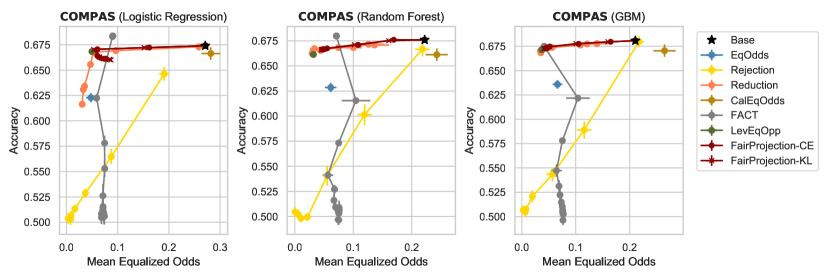
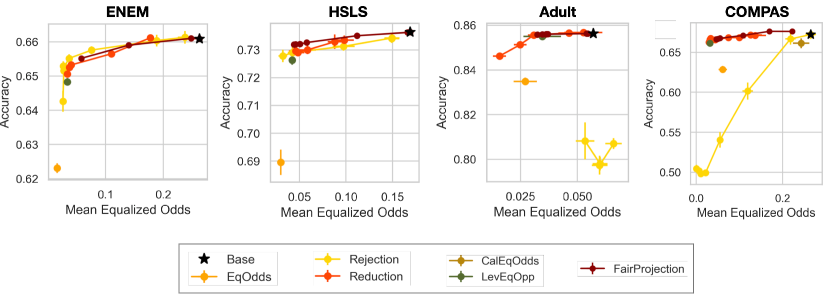
We compare our method with five existing fair learning algorithms: Reduction [5], reject-option classifier [44, Rejection], equalized-odds [35, EqOdds], calibrated equalized-odds [50, CalEqOdds], and leveraging equal opportunity [13, LevEqOpp].999https://github.com/lucaoneto/NIPS2019_Fairness. The choice of benchmarks is based on the availability of reproducible codes. For the first four baselines, we use IBM AIF360 library [8]. For Reduction and Rejection, we vary the tolerance to achieve different operation points on the fairness-accuracy trade-off curves. As EqOdds, CalEqOdds and LevEqOpp only allow hard equality constraint on equalized odds, they each produce a single point on the plot (see Fig. 1). We include the group attribute as a feature in the training set following the same benchmark procedure described in [5, 54] for a consistent comparison. Additional comparisons to [42] are given in Appendix B.3.1.
Refer to caption
Figure 1: Fairness-accuracy trade-off comparisons between FairProjection and five baselines on ENEM-50k-2C, HSLS, Adult and COMPAS datasets. For all methods, we used random forest as a base classifier.
Binary classification results.

We compare FairProjection with benchmarks tailored to binary classification in terms of the MEO-accuracy trade-off on the ENEM-50k-2C, HSLS, Adult, and COMPAS datasets in Fig. 1. Each point is obtained by averaging 10 runs with different train-test splits. FairProjection-CE curves were obtained by varying α𝛼\alpha values (cf. Table 2). When α=1.0𝛼1.0\alpha=1.0, the outputs of FairProjection-CE are equivalent to the base classifier RF.

We observe that FairProjection-CE and Reduction have the overall best and most consistent performances. On ENEM-50k-2C and HSLS datasets, although EqOdds achieves the best fairness, that fairness comes at the cost of 4%percent44\% accuracy drop (additively). The other four methods, on the other hand, produce comparatively good fairness with an accuracy loss of <1%absentpercent1<1\%. In particular, FairProjection-CE has the smallest accuracy drop whilst improving MEO from 0.17 to 0.04 on HSLS. CalEqOdds requires strict calibration requirements and yields inconsistent performance when these requirements are not met. On ENEM-50k-2C and HSLS, LevEqOpp achieves comparable MEO with a slight accuracy drop, and on COMPAS, LevEqOpp performs equally well as FairProjection-CE and Reduction. Note that with high fairness constraints (i.e., small tolerance), the accuracy of Rejection deteriorates.

Multi-Class results.

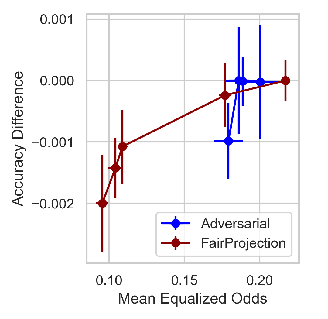
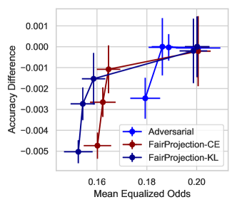
We illustrate how FairProjection performs on multi-class prediction using ENEM-50k-5C. In Figure 2, we plot fairness-accuracy trade-off of FairProjection-CE with logistic regression and adversarial debiasing [57, Adversarial]. As their base classifiers are different (Adversarial is a GAN-based method), we plot accuracy difference compared to the base classifier instead of plotting the absolute value of accuracy.101010Base accuracy for FairProjection=0.336absent0.336\ =0.336, Adversarial=0.307absent0.307\ =0.307. Random guessing accuracy=0.2absent0.2\ =0.2. FairProjection reduces MEO significantly with very small loss in accuracy. While Adversarial is also able to reduce MEO with negligible accuracy drop, it does not reduce the MEO as much as FairProjection. We show more extensive results with multi-group and multi-class (|𝒴|=5,=|𝒮|=5|\mathcal{Y}|=5,=|\mathcal{S}|=5) in Appendix B.3.2.

Refer to caption
Figure 2: Fairness-accuracy trade-off for multi-class prediction on ENEM-50k-5C. FairProjection is FairProjection-CE with LR base classifier.
Runtime comparisons.

In Table 3, we record the runtime of FairProjection-CE and-KL with the five benchmarks on ENEM-1.4M-2C. These experiments were run on a machine with AMD Ryzen 2990WX 64-thread 32-Core CPU and NVIDIA TITAN Xp 12-GB GPU. For consistency, we used the same fairness metric (MEO, α=0.01𝛼0.01\alpha=0.01), base classifier (GBM), and train/test split, and each number is the average of 2 repeated experiments. EqOdds, LevEqOpp, and CalEqOdds are faster than FairProjection since they are optimized to produce one trade-off point (cf. Fig. 1). Compared to baselines that produce full fairness-accuracy trade-off curves (i.e., Reduction and Rejection), FairProjection has the fastest runtime. Note that the 11.6 mins reported here for FairProjection-KL includes the time to fit the base classifiers. If base classifiers are pre-trained, the runtime of FairProjection-KL is 1.63 mins. Also, the non-parallel implementation of FairProjection-KL takes 25.3 mins—parallelization attains 15×\times speedup (detailed results in Appendix B.2).

Method Reduction Rejection EqOdds LevEqOpp CalEqOdds FairProjection (ours)
[5] [44] [35] [13] [50] CE KL
Runtime 223.6 16.9 5.9 7.9 5.3 11.3 11.6
Table 3: Execution time of FairProjection on the ENEM-1.4M-2C compared with five baseline methods (time shown in minutes). Methods in bold are capable of producing the full fairness-accuracy trade-off curves. Methods that are italicized have a uniformly superior performance.

6 Final remarks and limitations

We introduce a theoretically-grounded and versatile fairness intervention method, FairProjection, and showcase its favorable performance in extensive experiments. We encourage the reader to peruse our theoretical result in Appendix A and extensive additional numerical benchmarks in Appendix B. FairProjection is able to correct bias for multigroup/multiclass datasets, and it enjoys a fast runtime thanks to its parallelizability. We also evaluate our method on the ENEM dataset (see Appendix C for a detailed description of the dataset). Our benchmarks are a step forward in moving away from the overused COMPAS and UCI Adult datasets.

We only consider group-fairness, and it would be interesting to try to incorporate other fairness notions (e.g., individual fairness [26]) into our formulation. We assume that 𝒉basesuperscript𝒉base\boldsymbol{h}^{\mathrm{base}} is a pre-trained accurate (and potentially unfair) classifier; one future research direction is understanding how the accuracy of 𝒉basesuperscript𝒉base\boldsymbol{h}^{\mathrm{base}} influences the performance of the projected classifier. Finally, the performance of FairProjection is inherently constrained by data availability. Performance may degrade with intersectional increases of the number of groups, the number of labels, and the number of fairness constraints.

References

  • AAB+ [15] Martín Abadi, Ashish Agarwal, Paul Barham, Eugene Brevdo, Zhifeng Chen, Craig Citro, Greg S. Corrado, Andy Davis, Jeffrey Dean, Matthieu Devin, Sanjay Ghemawat, Ian Goodfellow, Andrew Harp, Geoffrey Irving, Michael Isard, Yangqing Jia, Rafal Jozefowicz, Lukasz Kaiser, Manjunath Kudlur, Josh Levenberg, Dandelion Mané, Rajat Monga, Sherry Moore, Derek Murray, Chris Olah, Mike Schuster, Jonathon Shlens, Benoit Steiner, Ilya Sutskever, Kunal Talwar, Paul Tucker, Vincent Vanhoucke, Vijay Vasudevan, Fernanda Viégas, Oriol Vinyals, Pete Warden, Martin Wattenberg, Martin Wicke, Yuan Yu, and Xiaoqiang Zheng. TensorFlow: Large-scale machine learning on heterogeneous systems, 2015. Software available from tensorflow.org.
  • AAV [19] Sina Aghaei, Mohammad Javad Azizi, and Phebe Vayanos. Learning optimal and fair decision trees for non-discriminative decision-making. In Proceedings of the AAAI Conference on Artificial Intelligence, volume 33, pages 1418–1426, 2019.
  • [3] Wael Alghamdi, Shahab Asoodeh, Hao Wang, Flavio P. Calmon, Dennis Wei, and Karthikeyan Natesan Ramamurthy. Model projection: Theory and applications to fair machine learning. In 2020 IEEE International Symposium on Information Theory (ISIT), pages 2711–2716, 2020.
  • [4] Wael Alghamdi, Shahab Asoodeh, Hao Wang, Flavio P. Calmon, Dennis Wei, and Karthikeyan Natesan Ramamurthy. Model projection: Theory and applications to fair machine learning. https://github.com/WaelAlghamdi/ModelProjection, 2020.
  • ABD+ [18] Alekh Agarwal, Alina Beygelzimer, Miroslav Dudík, John Langford, and Hanna Wallach. A reductions approach to fair classification. In International Conference on Machine Learning, pages 60–69. PMLR, 2018.
  • AHJ+ [22] Wael Alghamdi, Hsiang Hsu, Haewon Jeong, Hao Wang, P. Winston Michalak, Shahab Asoodeh, and Flavio du Pin Calmon. FairProjection. https://github.com/HsiangHsu/Fair-Projection, 2022.
  • ALMK [16] Julia Angwin, Jeff Larson, Surya Mattu, and Lauren Kirchner. Machine bias. ProPublica, 2016.
  • BDH+ [18] Rachel KE Bellamy, Kuntal Dey, Michael Hind, Samuel C Hoffman, Stephanie Houde, Kalapriya Kannan, Pranay Lohia, Jacquelyn Martino, Sameep Mehta, Aleksandra Mojsilovic, et al. Ai fairness 360: An extensible toolkit for detecting, understanding, and mitigating unwanted algorithmic bias. arXiv preprint arXiv:1810.01943, 2018.
  • BDNP [19] Maria-Florina F Balcan, Travis Dick, Ritesh Noothigattu, and Ariel D Procaccia. Envy-free classification. Advances in Neural Information Processing Systems, 32, 2019.
  • BFG [87] Jonathan M Borwein, SP Fitzpatrick, and JR Giles. The differentiability of real functions on normed linear space using generalized subgradients. Journal of mathematical analysis and applications, 128(2):512–534, 1987.
  • BPC+ [11] Stephen Boyd, Neal Parikh, Eric Chu, Borja Peleato, and Jonathan Eckstein. Distributed optimization and statistical learning via the alternating direction method of multipliers. Found. Trends Mach. Learn., 3(1):1–122, jan 2011.
  • BZZ+ [21] Michelle Bao, Angela Zhou, Samantha A Zottola, Brian Brubach, Sarah Desmarais, Aaron Seth Horowitz, Kristian Lum, and Suresh Venkatasubramanian. It’s COMPASlicated: The messy relationship between RAI datasets and algorithmic fairness benchmarks. In Thirty-fifth Conference on Neural Information Processing Systems Datasets and Benchmarks Track (Round 1), 2021.
  • CDH+ [19] Evgenii Chzhen, Christophe Denis, Mohamed Hebiri, Luca Oneto, and Massimiliano Pontil. Leveraging labeled and unlabeled data for consistent fair binary classification. Advances in Neural Information Processing Systems, 32, 2019.
  • CDPF+ [17] Sam Corbett-Davies, Emma Pierson, Avi Feller, Sharad Goel, and Aziz Huq. Algorithmic decision making and the cost of fairness. In Proceedings of the 23rd ACM SIGKDD International Conference on Knowledge Discovery and Data Mining, pages 797–806, 2017.
  • CHKV [19] L Elisa Celis, Lingxiao Huang, Vijay Keswani, and Nisheeth K Vishnoi. Classification with fairness constraints: A meta-algorithm with provable guarantees. In Proceedings of the conference on fairness, accountability, and transparency, pages 319–328, 2019.
  • Cho [17] Alexandra Chouldechova. Fair prediction with disparate impact: A study of bias in recidivism prediction instruments. Big data, 5(2):153–163, 2017.
  • CHS [20] Jaewoong Cho, Gyeongjo Hwang, and Changho Suh. A fair classifier using kernel density estimation. Advances in Neural Information Processing Systems, 33:15088–15099, 2020.
  • CJG+ [19] Andrew Cotter, Heinrich Jiang, Maya R Gupta, Serena Wang, Taman Narayan, Seungil You, and Karthik Sridharan. Optimization with non-differentiable constraints with applications to fairness, recall, churn, and other goals. J. Mach. Learn. Res., 20(172):1–59, 2019.
  • CKV [20] L Elisa Celis, Vijay Keswani, and Nisheeth Vishnoi. Data preprocessing to mitigate bias: A maximum entropy based approach. In International Conference on Machine Learning, pages 1349–1359. PMLR, 2020.
  • [20] Creative Commons. Creative commons attribution-noderivs 3.0 unported license. https://creativecommons.org/licenses/by-nd/3.0/deed.en. 05/25/2022.
  • Csi [75] Imre Csiszár. I-divergence geometry of probability distributions and minimization problems. The annals of probability, pages 146–158, 1975.
  • Csi [95] Imre Csiszár. Generalized projections for non-negative functions. In Proceedings of 1995 IEEE International Symposium on Information Theory, page 6. IEEE, 1995.
  • CST [17] Liang Chen, Defeng Sun, and Kim-Chuan Toh. A note on the convergence of admm for linearly constrained convex optimization problems. Comput. Optim. Appl., 66(2):327–343, mar 2017.
  • DEHH [21] Christophe Denis, Romuald Elie, Mohamed Hebiri, and François Hu. Fairness guarantee in multi-class classification. arXiv preprint arXiv:2109.13642, 2021.
  • DHMS [21] Frances Ding, Moritz Hardt, John Miller, and Ludwig Schmidt. Retiring adult: New datasets for fair machine learning. In M. Ranzato, A. Beygelzimer, Y. Dauphin, P.S. Liang, and J. Wortman Vaughan, editors, Advances in Neural Information Processing Systems, volume 34, pages 6478–6490. Curran Associates, Inc., 2021.
  • DHP+ [12] Cynthia Dwork, Moritz Hardt, Toniann Pitassi, Omer Reingold, and Richard Zemel. Fairness through awareness. In Proceedings of the 3rd innovations in theoretical computer science conference, pages 214–226, 2012.
  • DOBD+ [18] Michele Donini, Luca Oneto, Shai Ben-David, John Shawe-Taylor, and Massimiliano Pontil. Empirical risk minimization under fairness constraints. arXiv preprint arXiv:1802.08626, 2018.
  • DV [75] Monroe D Donsker and SR Srinivasa Varadhan. Asymptotic evaluation of certain markov process expectations for large time, i. Communications on Pure and Applied Mathematics, 28(1):1–47, 1975.
  • DY [16] Wei Deng and Wotao Yin. On the global and linear convergence of the generalized alternating direction method of multipliers. Journal of Scientific Computing, 66:889–916, 2016.
  • ET [99] Ivar Ekeland and Roger Témam. Convex analysis and variational problems. Classics in Applied Mathematics. Society for Industrial and Applied Mathematics, 1999.
  • FFM+ [15] Michael Feldman, Sorelle A Friedler, John Moeller, Carlos Scheidegger, and Suresh Venkatasubramanian. Certifying and removing disparate impact. In proceedings of the 21th ACM SIGKDD international conference on knowledge discovery and data mining, pages 259–268, 2015.
  • FSV+ [19] Sorelle A Friedler, Carlos Scheidegger, Suresh Venkatasubramanian, Sonam Choudhary, Evan P Hamilton, and Derek Roth. A comparative study of fairness-enhancing interventions in machine learning. In Proceedings of the conference on fairness, accountability, and transparency, pages 329–338, 2019.
  • GMV+ [21] Timnit Gebru, Jamie Morgenstern, Briana Vecchione, Jennifer Wortman Vaughan, Hanna Wallach, Hal Daumé Iii, and Kate Crawford. Datasheets for datasets. Communications of the ACM, 64(12):86–92, 2021.
  • GP [17] Bolin Gao and Lacra Pavel. On the properties of the softmax function with application in game theory and reinforcement learning. arXiv preprint arXiv:1704.00805, 2017.
  • HPS [16] Moritz Hardt, Eric Price, and Nati Srebro. Equality of opportunity in supervised learning. Advances in neural information processing systems, 29:3315–3323, 2016.
  • HR [19] Bruce Hajek and Maxim Raginsky. Statistical learning theory. Lecture Notes, 387, 2019.
  • INE [20] INEP. Instituto nacional de estudos e pesquisas educaionais anísio teixeira, microdados do ENEM. https://www.gov.br/inep/pt-br/acesso-a-informacao/dados-abertos/microdados/enem, 2020. Accessed: 2022-05-23.
  • IPH+ [11] Steven J Ingels, Daniel J Pratt, Deborah R Herget, Laura J Burns, Jill A Dever, Randolph Ottem, James E Rogers, Ying Jin, and Steve Leinwand. High school longitudinal study of 2009 (hsls: 09): Base-year data file documentation. nces 2011-328. National Center for Education Statistics, 2011.
  • JN [20] Heinrich Jiang and Ofir Nachum. Identifying and correcting label bias in machine learning. In International Conference on Artificial Intelligence and Statistics, pages 702–712. PMLR, 2020.
  • JSW [22] Taeuk Jang, Pengyi Shi, and Xiaoqian Wang. Group-aware threshold adaptation for fair classification. Proceedings of the AAAI Conference on Artificial Intelligence, 2022.
  • JWC [22] Haewon Jeong, Hao Wang, and Flavio Calmon. Fairness without imputation: A decision tree approach for fair prediction with missing values. In Proceedings of the AAAI Conference on Artificial Intelligence, 2022.
  • KCT [20] Joon Sik Kim, Jiahao Chen, and Ameet Talwalkar. FACT: A diagnostic for group fairness trade-offs. In International Conference on Machine Learning, pages 5264–5274. PMLR, 2020.
  • KJW+ [21] Anilesh Krishnaswamy, Zhihao Jiang, Kangning Wang, Yu Cheng, and Kamesh Munagala. Fair for all: Best-effort fairness guarantees for classification. In International Conference on Artificial Intelligence and Statistics, pages 3259–3267. PMLR, 2021.
  • KKZ [12] F. Kamiran, A. Karim, and X. Zhang. Decision theory for discrimination-aware classification. In 2012 IEEE 12th International Conference on Data Mining, pages 924–929, Dec 2012.
  • KS [15] M Ashok Kumar and Rajesh Sundaresan. Minimization problems based on relative α𝛼\alpha-entropy i: Forward projection. IEEE Transactions on Information Theory, 61(9):5063–5080, 2015.
  • KS [16] M Ashok Kumar and Igal Sason. Projection theorems for the rényi divergence on α𝛼\alpha-convex sets. IEEE Transactions on Information Theory, 62(9):4924–4935, 2016.
  • Lic [13] M. Lichman. UCI machine learning repository, 2013.
  • MW [18] Aditya Krishna Menon and Robert C Williamson. The cost of fairness in binary classification. In Conference on Fairness, Accountability and Transparency, pages 107–118. PMLR, 2018.
  • Nes [04] Y. Nesterov. Introductory Lectures on Convex Optimization. Springer, Boston, MA, 2004.
  • PRW+ [17] Geoff Pleiss, Manish Raghavan, Felix Wu, Jon Kleinberg, and Kilian Q Weinberger. On fairness and calibration. arXiv preprint arXiv:1709.02012, 2017.
  • PVG+ [11] Fabian Pedregosa, Gaël Varoquaux, Alexandre Gramfort, Vincent Michel, Bertrand Thirion, Olivier Grisel, Mathieu Blondel, Peter Prettenhofer, Ron Weiss, Vincent Dubourg, et al. Scikit-learn: Machine learning in python. the Journal of machine Learning research, 12:2825–2830, 2011.
  • Roc [09] R. Tyrrell Rockafellar. Variational analysis. Grundlehren der mathematischen Wissenschaften ; 317. Springer, Berlin ; Heidelberg, 1st ed. 1998. edition, 2009.
  • WRC [20] Dennis Wei, Karthikeyan Natesan Ramamurthy, and Flavio P Calmon. Optimized score transformation for fair classification. In 23rd International Conference on Artificial Intelligence and Statistics, 2020.
  • WRC [21] Dennis Wei, Karthikeyan Natesan Ramamurthy, and Flavio P Calmon. Optimized score transformation for consistent fair classification. Journal of Machine Learning Research, 22(258):1–78, 2021.
  • YCK [20] Forest Yang, Mouhamadou Cisse, and Oluwasanmi O Koyejo. Fairness with overlapping groups; a probabilistic perspective. Advances in Neural Information Processing Systems, 33, 2020.
  • YX [20] Qing Ye and Weijun Xie. Unbiased subdata selection for fair classification: A unified framework and scalable algorithms. arXiv preprint arXiv:2012.12356, 2020.
  • ZLM [18] Brian Hu Zhang, Blake Lemoine, and Margaret Mitchell. Mitigating unwanted biases with adversarial learning. In Proceedings of the 2018 AAAI/ACM Conference on AI, Ethics, and Society, pages 335–340, 2018.
  • ZVRG [17] Muhammad Bilal Zafar, Isabel Valera, Manuel Gomez Rogriguez, and Krishna P Gummadi. Fairness constraints: Mechanisms for fair classification. In Artificial Intelligence and Statistics, pages 962–970, 2017.

Appendix

This appendix is divided into three parts: Appendix A: Proofs of theoretical results; Appendix B: More details on the experimental setup, additional quantitative experiments, and more qualitative comparisons with related work; and Appendix C: A datasheet for ENEM (2020) dataset.

Appendix A Proofs of theoretical results

The theoretical details of our work are included in this appendix. We prove the strong duality stated in Theorem 2 in Appendix A.1. Algorithm 1 is derived in Appendix A.2. The inner iterations of Algorithm 1 are further developed in Appendices A.3A.4. The convergence rate results in Theorems 34 are proved in Appendices A.5A.6. Explicit formulas for the 𝑮𝑮\boldsymbol{G} matrix induced by the fairness metrics in Table 2 are given in Appendix A.7.

A.1 Proof of Theorem 2: strong duality

We use the following minimax theorem, which is a generalization of Sion’s minimax theorem.

Theorem 5 ([30, Chapter VI, Prop. 2.2]).

Let V𝑉V and Z𝑍Z be two reflexive Banach spaces, and fix two convex, closed, and non-empty subsets 𝒜V𝒜𝑉\mathcal{A}\subset V and Z𝑍\mathcal{B}\subset Z. Let L:𝒜×:𝐿𝒜L:\mathcal{A}\times\mathcal{B}\to\mathbb{R} be a function such that for each u𝒜𝑢𝒜u\in\mathcal{A} the function pL(u,p)maps-to𝑝𝐿𝑢𝑝p\mapsto L(u,p) is concave and upper semicontinuous, and for each p𝑝p\in\mathcal{B} the function uL(u,p)maps-to𝑢𝐿𝑢𝑝u\mapsto L(u,p) is convex and lower semicontinuous. Suppose that there exist points u0𝒜subscript𝑢0𝒜u_{0}\in\mathcal{A} and p0subscript𝑝0p_{0}\in\mathcal{B} such that limp,pL(u0,p)=subscriptformulae-sequence𝑝norm𝑝𝐿subscript𝑢0𝑝\lim_{p\in\mathcal{B},\|p\|\to\infty}L(u_{0},p)=-\infty and limu𝒜,uL(u,p0)=subscriptformulae-sequence𝑢𝒜norm𝑢𝐿𝑢subscript𝑝0\lim_{u\in\mathcal{A},\|u\|\to\infty}L(u,p_{0})=\infty. Then, L𝐿L has at least one saddle-point (u¯,p¯)¯𝑢¯𝑝(\overline{u},\overline{p}), and

L(u¯,p¯)=minu𝒜suppL(u,p)=maxpinfu𝒜L(u,p).𝐿¯𝑢¯𝑝subscript𝑢𝒜subscriptsupremum𝑝𝐿𝑢𝑝subscript𝑝subscriptinfimum𝑢𝒜𝐿𝑢𝑝L(\overline{u},\overline{p})=\min_{u\in\mathcal{A}}\ \sup_{p\in\mathcal{B}}\ L(u,p)=\max_{p\in\mathcal{B}}\ \inf_{u\in\mathcal{A}}\ L(u,p). (12)

In particular, in (12), there exists a minimizer in 𝒜𝒜\mathcal{A} of the outer minimization, and a maximizer in \mathcal{B} of the outer maximization.

Denote 𝒉i𝒉(Xi)subscript𝒉𝑖𝒉subscript𝑋𝑖\boldsymbol{h}_{i}\triangleq\boldsymbol{h}(X_{i}), 𝒑i𝒉base(Xi)subscript𝒑𝑖superscript𝒉basesubscript𝑋𝑖\boldsymbol{p}_{i}\triangleq\boldsymbol{h}^{\mathrm{base}}(X_{i}), 𝒂i𝒂(Xi)subscript𝒂𝑖𝒂subscript𝑋𝑖\boldsymbol{a}_{i}\triangleq\boldsymbol{a}(X_{i}), and 𝑮i𝑮(Xi)subscript𝑮𝑖𝑮subscript𝑋𝑖\boldsymbol{G}_{i}\triangleq\boldsymbol{G}(X_{i}), and let the matrix 𝓖N(𝑮1/N,,𝑮N/N,𝑰K)K×(NC+K)subscript𝓖𝑁subscript𝑮1𝑁subscript𝑮𝑁𝑁subscript𝑰𝐾superscript𝐾𝑁𝐶𝐾\boldsymbol{\mathcal{G}}_{N}\triangleq\left(\boldsymbol{G}_{1}/\sqrt{N},\cdots,\boldsymbol{G}_{N}/\sqrt{N},\boldsymbol{I}_{K}\right)\in\mathbb{R}^{K\times(NC+K)} be as in the theorem statement. We may rewrite the optimization (6) as

minimize(𝒉i,𝒂i,𝒃)𝚫C×C×K,i[N]formulae-sequencesubscript𝒉𝑖subscript𝒂𝑖𝒃subscript𝚫𝐶superscript𝐶superscript𝐾𝑖delimited-[]𝑁minimize\displaystyle\underset{\begin{subarray}{c}(\boldsymbol{h}_{i},\boldsymbol{a}_{i},\boldsymbol{b})\in\mathbf{\Delta}_{C}\times\mathbb{R}^{C}\times\mathbb{R}^{K},i\in[N]\end{subarray}}{\textup{minimize}} 1Ni[N]Df(𝒉i𝒑i)+τ1(𝒂i22+𝒃22)1𝑁subscript𝑖delimited-[]𝑁subscript𝐷𝑓conditionalsubscript𝒉𝑖subscript𝒑𝑖subscript𝜏1superscriptsubscriptnormsubscript𝒂𝑖22superscriptsubscriptnorm𝒃22\displaystyle\frac{1}{N}\sum_{i\in[N]}D_{f}\left(\boldsymbol{h}_{i}\|\boldsymbol{p}_{i}\right)+\tau_{1}\cdot\left(\|\boldsymbol{a}_{i}\|_{2}^{2}+\|\boldsymbol{b}\|_{2}^{2}\right) (13)
subject to 1Ni[N]𝑮i𝒉i+τ2(𝑮i𝒂i𝒃)𝟎.1𝑁subscript𝑖delimited-[]𝑁subscript𝑮𝑖subscript𝒉𝑖subscript𝜏2subscript𝑮𝑖subscript𝒂𝑖𝒃0\displaystyle\frac{1}{N}\sum_{i\in[N]}\boldsymbol{G}_{i}\boldsymbol{h}_{i}+\tau_{2}\cdot\left(\boldsymbol{G}_{i}\boldsymbol{a}_{i}-\boldsymbol{b}\right)\leq\mathbf{0}.

We define f𝑓f at 00 by the right limit f(0)f(0+)𝑓0𝑓limit-from0f(0)\triangleq f(0+). Assume for now that f(0+)<𝑓limit-from0f(0+)<\infty, and we will explain at the end of this proof how to treat the case f(0+)=𝑓limit-from0f(0+)=\infty. For the optimization problem (13), the Lagrangian L:𝚫CN×NC×K×+K:𝐿superscriptsubscript𝚫𝐶𝑁superscript𝑁𝐶superscript𝐾superscriptsubscript𝐾L:\mathbf{\Delta}_{C}^{N}\times\mathbb{R}^{NC}\times\mathbb{R}^{K}\times\mathbb{R}_{+}^{K}\to\mathbb{R} is given by

L((𝒉i)i[N],(𝒂i)i[N],𝒃,𝝀)1Ni[N]Df(𝒉i𝒑i)𝐿subscriptsubscript𝒉𝑖𝑖delimited-[]𝑁subscriptsubscript𝒂𝑖𝑖delimited-[]𝑁𝒃𝝀1𝑁subscript𝑖delimited-[]𝑁subscript𝐷𝑓conditionalsubscript𝒉𝑖subscript𝒑𝑖\displaystyle L\left(\left(\boldsymbol{h}_{i}\right)_{i\in[N]},\left(\boldsymbol{a}_{i}\right)_{i\in[N]},\boldsymbol{b},\boldsymbol{\lambda}\right)\triangleq\frac{1}{N}\sum_{i\in[N]}D_{f}\left(\boldsymbol{h}_{i}\|\boldsymbol{p}_{i}\right) +τ1(𝒂i22+𝒃22)subscript𝜏1superscriptsubscriptnormsubscript𝒂𝑖22superscriptsubscriptnorm𝒃22\displaystyle+\tau_{1}\left(\|\boldsymbol{a}_{i}\|_{2}^{2}+\|\boldsymbol{b}\|_{2}^{2}\right) (14)
+𝝀T(𝑮i𝒉i+τ2(𝑮i𝒂i𝒃)).superscript𝝀𝑇subscript𝑮𝑖subscript𝒉𝑖subscript𝜏2subscript𝑮𝑖subscript𝒂𝑖𝒃\displaystyle+\boldsymbol{\lambda}^{T}\left(\boldsymbol{G}_{i}\boldsymbol{h}_{i}+\tau_{2}\left(\boldsymbol{G}_{i}\boldsymbol{a}_{i}-\boldsymbol{b}\right)\right).

With 𝒗(x;𝝀)𝑮(x)T𝝀𝒗𝑥𝝀𝑮superscript𝑥𝑇𝝀\boldsymbol{v}(x;\boldsymbol{\lambda})\triangleq-\boldsymbol{G}(x)^{T}\boldsymbol{\lambda} as in the theorem statement, and denoting 𝒗i𝒗(Xi;𝝀)=𝑮iT𝝀subscript𝒗𝑖𝒗subscript𝑋𝑖𝝀superscriptsubscript𝑮𝑖𝑇𝝀\boldsymbol{v}_{i}\triangleq\boldsymbol{v}(X_{i};\boldsymbol{\lambda})=-\boldsymbol{G}_{i}^{T}\boldsymbol{\lambda}, we may rewrite the Lagrangian as

L((𝒉i)i[N],(𝒂i)i[N],𝒃,𝝀)=1Ni[N]Df(𝒉i𝒑i)𝐿subscriptsubscript𝒉𝑖𝑖delimited-[]𝑁subscriptsubscript𝒂𝑖𝑖delimited-[]𝑁𝒃𝝀1𝑁subscript𝑖delimited-[]𝑁subscript𝐷𝑓conditionalsubscript𝒉𝑖subscript𝒑𝑖\displaystyle L\left(\left(\boldsymbol{h}_{i}\right)_{i\in[N]},\left(\boldsymbol{a}_{i}\right)_{i\in[N]},\boldsymbol{b},\boldsymbol{\lambda}\right)=\frac{1}{N}\sum_{i\in[N]}D_{f}\left(\boldsymbol{h}_{i}\|\boldsymbol{p}_{i}\right) 𝒗iT𝒉i+τ1𝒂i22τ2𝒗iT𝒂isuperscriptsubscript𝒗𝑖𝑇subscript𝒉𝑖subscript𝜏1superscriptsubscriptnormsubscript𝒂𝑖22subscript𝜏2superscriptsubscript𝒗𝑖𝑇subscript𝒂𝑖\displaystyle-\boldsymbol{v}_{i}^{T}\boldsymbol{h}_{i}+\tau_{1}\|\boldsymbol{a}_{i}\|_{2}^{2}-\tau_{2}\boldsymbol{v}_{i}^{T}\boldsymbol{a}_{i} (15)
+τ1𝒃22τ2𝝀T𝒃.subscript𝜏1superscriptsubscriptnorm𝒃22subscript𝜏2superscript𝝀𝑇𝒃\displaystyle+\tau_{1}\|\boldsymbol{b}\|_{2}^{2}-\tau_{2}\boldsymbol{\lambda}^{T}\boldsymbol{b}.

The optimization problem (13) can be written as

inf(𝒉i,𝒂i,𝒃)𝚫C×C×K,i[N]sup𝝀+KL((𝒉i)i[N],(𝒂i)i[N],𝒃,𝝀).subscriptinfimumformulae-sequencesubscript𝒉𝑖subscript𝒂𝑖𝒃subscript𝚫𝐶superscript𝐶superscript𝐾𝑖delimited-[]𝑁subscriptsupremum𝝀superscriptsubscript𝐾𝐿subscriptsubscript𝒉𝑖𝑖delimited-[]𝑁subscriptsubscript𝒂𝑖𝑖delimited-[]𝑁𝒃𝝀\inf_{(\boldsymbol{h}_{i},\boldsymbol{a}_{i},\boldsymbol{b})\in\mathbf{\Delta}_{C}\times\mathbb{R}^{C}\times\mathbb{R}^{K},i\in[N]}\ \sup_{\boldsymbol{\lambda}\in\mathbb{R}_{+}^{K}}\ L\left(\left(\boldsymbol{h}_{i}\right)_{i\in[N]},\left(\boldsymbol{a}_{i}\right)_{i\in[N]},\boldsymbol{b},\boldsymbol{\lambda}\right). (16)

We check that the Lagrangian L𝐿L satisfies the conditions in Theorem 5. First, any Euclidean space Msuperscript𝑀\mathbb{R}^{M} (for M𝑀M\in\mathbb{N}) is a reflexive Banach space since it is finite-dimensional. In addition, the convex nonempty sets 𝚫CN×NC×Ksuperscriptsubscript𝚫𝐶𝑁superscript𝑁𝐶superscript𝐾\mathbf{\Delta}_{C}^{N}\times\mathbb{R}^{NC}\times\mathbb{R}^{K} and +Ksuperscriptsubscript𝐾\mathbb{R}_{+}^{K} are closed in their respective ambient Euclidean spaces. By continuity and convexity of f𝑓f, and linearity of L𝐿L in 𝝀𝝀\boldsymbol{\lambda}, we have that L𝐿L satisfies all the convexity, concavity, and semicontinuity conditions in Theorem 5. Further, fixing any 𝒉i𝚫Csubscript𝒉𝑖subscript𝚫𝐶\boldsymbol{h}_{i}\in\mathbf{\Delta}_{C}, i[N]𝑖delimited-[]𝑁i\in[N], and letting 𝒂i=𝟎subscript𝒂𝑖0\boldsymbol{a}_{i}=\mathbf{0}, i[N]𝑖delimited-[]𝑁i\in[N], and 𝒃=1τ2(𝟏+1Ni[N]𝑮i𝒉i)𝒃1subscript𝜏211𝑁subscript𝑖delimited-[]𝑁subscript𝑮𝑖subscript𝒉𝑖\boldsymbol{b}=\frac{1}{\tau_{2}}\left(\mathbf{1}+\frac{1}{N}\sum_{i\in[N]}\boldsymbol{G}_{i}\boldsymbol{h}_{i}\right), we would get that

L((𝒉i)i[N],(𝒂i)i[N],𝒃,𝝀)=𝝀T𝟏+1Ni[N]Df(𝒉i𝒑i)+τ1𝒃22as𝝀2.formulae-sequence𝐿subscriptsubscript𝒉𝑖𝑖delimited-[]𝑁subscriptsubscript𝒂𝑖𝑖delimited-[]𝑁𝒃𝝀superscript𝝀𝑇11𝑁subscript𝑖delimited-[]𝑁subscript𝐷𝑓conditionalsubscript𝒉𝑖subscript𝒑𝑖subscript𝜏1superscriptsubscriptnorm𝒃22assubscriptnorm𝝀2L\left(\left(\boldsymbol{h}_{i}\right)_{i\in[N]},\left(\boldsymbol{a}_{i}\right)_{i\in[N]},\boldsymbol{b},\boldsymbol{\lambda}\right)=-\boldsymbol{\lambda}^{T}\mathbf{1}+\frac{1}{N}\sum_{i\in[N]}D_{f}\left(\boldsymbol{h}_{i}\|\boldsymbol{p}_{i}\right)+\tau_{1}\|\boldsymbol{b}\|_{2}^{2}\to-\infty\quad\text{as}\quad\|\boldsymbol{\lambda}\|_{2}\to\infty. (17)

In addition, choosing 𝝀=𝟎𝝀0\boldsymbol{\lambda}=\mathbf{0}, we have the Lagrangian

L((𝒉i)i[N],(𝒂i)i[N],𝒃,𝝀)=1Ni[N]Df(𝒉i𝒑i)𝐿subscriptsubscript𝒉𝑖𝑖delimited-[]𝑁subscriptsubscript𝒂𝑖𝑖delimited-[]𝑁𝒃𝝀1𝑁subscript𝑖delimited-[]𝑁subscript𝐷𝑓conditionalsubscript𝒉𝑖subscript𝒑𝑖\displaystyle L\left(\left(\boldsymbol{h}_{i}\right)_{i\in[N]},\left(\boldsymbol{a}_{i}\right)_{i\in[N]},\boldsymbol{b},\boldsymbol{\lambda}\right)=\frac{1}{N}\sum_{i\in[N]}D_{f}\left(\boldsymbol{h}_{i}\|\boldsymbol{p}_{i}\right) +τ1𝒂i22+τ1𝒃22subscript𝜏1superscriptsubscriptnormsubscript𝒂𝑖22subscript𝜏1superscriptsubscriptnorm𝒃22\displaystyle+\tau_{1}\|\boldsymbol{a}_{i}\|_{2}^{2}+\tau_{1}\|\boldsymbol{b}\|_{2}^{2}\to\infty (18)

as 𝒃2+i[N]𝒉i2+𝒂i2subscriptnorm𝒃2subscript𝑖delimited-[]𝑁subscriptnormsubscript𝒉𝑖2subscriptnormsubscript𝒂𝑖2\|\boldsymbol{b}\|_{2}+\sum_{i\in[N]}\|\boldsymbol{h}_{i}\|_{2}+\|\boldsymbol{a}_{i}\|_{2}\to\infty. Thus, we may apply the minimax result in Theorem 5 to obtain the existence of a saddle-point of L𝐿L and that

min(𝒉i,𝒂i,𝒃)𝚫C×C×K,i[N]subscriptformulae-sequencesubscript𝒉𝑖subscript𝒂𝑖𝒃subscript𝚫𝐶superscript𝐶superscript𝐾𝑖delimited-[]𝑁\displaystyle\min_{(\boldsymbol{h}_{i},\boldsymbol{a}_{i},\boldsymbol{b})\in\mathbf{\Delta}_{C}\times\mathbb{R}^{C}\times\mathbb{R}^{K},i\in[N]} sup𝝀+KL((𝒉i)i[N],(𝒂i)i[N],𝒃,𝝀)subscriptsupremum𝝀superscriptsubscript𝐾𝐿subscriptsubscript𝒉𝑖𝑖delimited-[]𝑁subscriptsubscript𝒂𝑖𝑖delimited-[]𝑁𝒃𝝀\displaystyle\sup_{\boldsymbol{\lambda}\in\mathbb{R}_{+}^{K}}\ L\left(\left(\boldsymbol{h}_{i}\right)_{i\in[N]},\left(\boldsymbol{a}_{i}\right)_{i\in[N]},\boldsymbol{b},\boldsymbol{\lambda}\right) (19)
=max𝝀+Kinf(𝒉i,𝒂i,𝒃)𝚫C×C×K,i[N]L((𝒉i)i[N],(𝒂i)i[N],𝒃,𝝀).absentsubscript𝝀superscriptsubscript𝐾subscriptinfimumformulae-sequencesubscript𝒉𝑖subscript𝒂𝑖𝒃subscript𝚫𝐶superscript𝐶superscript𝐾𝑖delimited-[]𝑁𝐿subscriptsubscript𝒉𝑖𝑖delimited-[]𝑁subscriptsubscript𝒂𝑖𝑖delimited-[]𝑁𝒃𝝀\displaystyle=\max_{\boldsymbol{\lambda}\in\mathbb{R}_{+}^{K}}\ \inf_{(\boldsymbol{h}_{i},\boldsymbol{a}_{i},\boldsymbol{b})\in\mathbf{\Delta}_{C}\times\mathbb{R}^{C}\times\mathbb{R}^{K},i\in[N]}\ L\left(\left(\boldsymbol{h}_{i}\right)_{i\in[N]},\left(\boldsymbol{a}_{i}\right)_{i\in[N]},\boldsymbol{b},\boldsymbol{\lambda}\right).

In particular, there exists a minimizer (𝒉iopt,N,𝒂iopt,N,𝒃opt,N)𝚫C×C×K,i[N]formulae-sequencesuperscriptsubscript𝒉𝑖opt𝑁superscriptsubscript𝒂𝑖opt𝑁superscript𝒃opt𝑁subscript𝚫𝐶superscript𝐶superscript𝐾𝑖delimited-[]𝑁(\boldsymbol{h}_{i}^{\mathrm{opt},N},\boldsymbol{a}_{i}^{\mathrm{opt},N},\boldsymbol{b}^{\mathrm{opt},N})\in\mathbf{\Delta}_{C}\times\mathbb{R}^{C}\times\mathbb{R}^{K},i\in[N], of the outer minimization in the left-hand side in (19), and a maximizer 𝝀+Ksuperscript𝝀superscriptsubscript𝐾\boldsymbol{\lambda}^{\star}\in\mathbb{R}_{+}^{K} of the outer maximization in the right-hand side of (19). By strict convexity of the objective function in (13) (and convexity of the feasibility set), we obtain that the minimizer (𝒉iopt,N,𝒂iopt,N,𝒃opt,N)𝚫C×C×K,i[N]formulae-sequencesuperscriptsubscript𝒉𝑖opt𝑁superscriptsubscript𝒂𝑖opt𝑁superscript𝒃opt𝑁subscript𝚫𝐶superscript𝐶superscript𝐾𝑖delimited-[]𝑁(\boldsymbol{h}_{i}^{\mathrm{opt},N},\boldsymbol{a}_{i}^{\mathrm{opt},N},\boldsymbol{b}^{\mathrm{opt},N})\in\mathbf{\Delta}_{C}\times\mathbb{R}^{C}\times\mathbb{R}^{K},i\in[N], is unique. We show next that the optimizer 𝝀superscript𝝀\boldsymbol{\lambda}^{\star} is unique too, which we will denote by 𝝀ζ,Nsuperscriptsubscript𝝀𝜁𝑁\boldsymbol{\lambda}_{\zeta,N}^{\star} as in the theorem statement. We also show that, for each fixed 𝝀+K𝝀superscriptsubscript𝐾\boldsymbol{\lambda}\in\mathbb{R}_{+}^{K}, there is a unique minimizer (𝒉i𝝀,𝒂i𝝀,𝒃𝝀)𝚫C×C×K,i[N]formulae-sequencesuperscriptsubscript𝒉𝑖𝝀superscriptsubscript𝒂𝑖𝝀superscript𝒃𝝀subscript𝚫𝐶superscript𝐶superscript𝐾𝑖delimited-[]𝑁(\boldsymbol{h}_{i}^{\boldsymbol{\lambda}},\boldsymbol{a}_{i}^{\boldsymbol{\lambda}},\boldsymbol{b}^{\boldsymbol{\lambda}})\in\mathbf{\Delta}_{C}\times\mathbb{R}^{C}\times\mathbb{R}^{K},i\in[N], of the inner minimization in the right-hand side of (19); by strict convexity of f𝑓f, this would imply that 𝒉iopt,N=𝒉i𝝀ζ,Nsuperscriptsubscript𝒉𝑖opt𝑁superscriptsubscript𝒉𝑖subscriptsuperscript𝝀𝜁𝑁\boldsymbol{h}_{i}^{\mathrm{opt},N}=\boldsymbol{h}_{i}^{\boldsymbol{\lambda}^{\star}_{\zeta,N}}.

Now, fix 𝝀+K𝝀superscriptsubscript𝐾\boldsymbol{\lambda}\in\mathbb{R}_{+}^{K}, and consider the inner minimization in (19). We have that

inf(𝒉i,𝒂i,𝒃)𝚫C×C×K,i[N]L((𝒉i)i[N],(𝒂i)i[N],𝒃,𝝀)subscriptinfimumformulae-sequencesubscript𝒉𝑖subscript𝒂𝑖𝒃subscript𝚫𝐶superscript𝐶superscript𝐾𝑖delimited-[]𝑁𝐿subscriptsubscript𝒉𝑖𝑖delimited-[]𝑁subscriptsubscript𝒂𝑖𝑖delimited-[]𝑁𝒃𝝀\displaystyle\inf_{(\boldsymbol{h}_{i},\boldsymbol{a}_{i},\boldsymbol{b})\in\mathbf{\Delta}_{C}\times\mathbb{R}^{C}\times\mathbb{R}^{K},i\in[N]}\ L\left(\left(\boldsymbol{h}_{i}\right)_{i\in[N]},\left(\boldsymbol{a}_{i}\right)_{i\in[N]},\boldsymbol{b},\boldsymbol{\lambda}\right)
=inf(𝒉i,𝒂i,𝒃)𝚫C×C×K,i[N]1Ni[N]Df(𝒉i𝒑i)𝒗iT𝒉i+τ1𝒂i22τ2𝒗iT𝒂i+τ1𝒃22τ2𝝀T𝒃absentsubscriptinfimumformulae-sequencesubscript𝒉𝑖subscript𝒂𝑖𝒃subscript𝚫𝐶superscript𝐶superscript𝐾𝑖delimited-[]𝑁1𝑁subscript𝑖delimited-[]𝑁subscript𝐷𝑓conditionalsubscript𝒉𝑖subscript𝒑𝑖superscriptsubscript𝒗𝑖𝑇subscript𝒉𝑖subscript𝜏1superscriptsubscriptnormsubscript𝒂𝑖22subscript𝜏2superscriptsubscript𝒗𝑖𝑇subscript𝒂𝑖subscript𝜏1superscriptsubscriptnorm𝒃22subscript𝜏2superscript𝝀𝑇𝒃\displaystyle=\inf_{(\boldsymbol{h}_{i},\boldsymbol{a}_{i},\boldsymbol{b})\in\mathbf{\Delta}_{C}\times\mathbb{R}^{C}\times\mathbb{R}^{K},i\in[N]}\frac{1}{N}\sum_{i\in[N]}D_{f}\left(\boldsymbol{h}_{i}\|\boldsymbol{p}_{i}\right)-\boldsymbol{v}_{i}^{T}\boldsymbol{h}_{i}+\tau_{1}\|\boldsymbol{a}_{i}\|_{2}^{2}-\tau_{2}\boldsymbol{v}_{i}^{T}\boldsymbol{a}_{i}+\tau_{1}\|\boldsymbol{b}\|_{2}^{2}-\tau_{2}\boldsymbol{\lambda}^{T}\boldsymbol{b} (20)
=1Ni[N]inf𝒉i𝚫CDf(𝒉i𝒑i)𝒗iT𝒉i+inf𝒂iCτ1𝒂i22τ2𝒗iT𝒂i+inf𝒃Kτ1𝒃22τ2𝝀T𝒃absent1𝑁subscript𝑖delimited-[]𝑁subscriptinfimumsubscript𝒉𝑖subscript𝚫𝐶subscript𝐷𝑓conditionalsubscript𝒉𝑖subscript𝒑𝑖superscriptsubscript𝒗𝑖𝑇subscript𝒉𝑖subscriptinfimumsubscript𝒂𝑖superscript𝐶subscript𝜏1superscriptsubscriptnormsubscript𝒂𝑖22subscript𝜏2superscriptsubscript𝒗𝑖𝑇subscript𝒂𝑖subscriptinfimum𝒃superscript𝐾subscript𝜏1superscriptsubscriptnorm𝒃22subscript𝜏2superscript𝝀𝑇𝒃\displaystyle=\frac{1}{N}\sum_{i\in[N]}\inf_{\begin{subarray}{c}\boldsymbol{h}_{i}\in\mathbf{\Delta}_{C}\end{subarray}}D_{f}(\boldsymbol{h}_{i}\|\boldsymbol{p}_{i})-\boldsymbol{v}_{i}^{T}\boldsymbol{h}_{i}+\inf_{\boldsymbol{a}_{i}\in\mathbb{R}^{C}}\tau_{1}\|\boldsymbol{a}_{i}\|_{2}^{2}-\tau_{2}\boldsymbol{v}_{i}^{T}\boldsymbol{a}_{i}+\inf_{\boldsymbol{b}\in\mathbb{R}^{K}}\tau_{1}\|\boldsymbol{b}\|_{2}^{2}-\tau_{2}\boldsymbol{\lambda}^{T}\boldsymbol{b} (21)
=1Ni[N]Dfconj(𝒗i,𝒑i)12ζ𝒗i2212ζ𝝀22absent1𝑁subscript𝑖delimited-[]𝑁superscriptsubscript𝐷𝑓conjsubscript𝒗𝑖subscript𝒑𝑖12𝜁superscriptsubscriptnormsubscript𝒗𝑖2212𝜁superscriptsubscriptnorm𝝀22\displaystyle=\frac{1}{N}\sum_{i\in[N]}-D_{f}^{\mathrm{conj}}(\boldsymbol{v}_{i},\boldsymbol{p}_{i})-\frac{1}{2}\zeta\|\boldsymbol{v}_{i}\|_{2}^{2}-\frac{1}{2}\zeta\|\boldsymbol{\lambda}\|_{2}^{2} (22)
=ζ2𝓖NT𝝀221Ni[N]Dfconj(𝒗i,𝒑i)absent𝜁2superscriptsubscriptnormsuperscriptsubscript𝓖𝑁𝑇𝝀221𝑁subscript𝑖delimited-[]𝑁superscriptsubscript𝐷𝑓conjsubscript𝒗𝑖subscript𝒑𝑖\displaystyle=-\frac{\zeta}{2}\left\|\boldsymbol{\mathcal{G}}_{N}^{T}\boldsymbol{\lambda}\right\|_{2}^{2}-\frac{1}{N}\sum_{i\in[N]}D_{f}^{\mathrm{conj}}(\boldsymbol{v}_{i},\boldsymbol{p}_{i}) (23)

where ζτ22/(2τ1)𝜁superscriptsubscript𝜏222subscript𝜏1\zeta\triangleq\tau_{2}^{2}/(2\tau_{1}). Here, the minimizers are 𝒂i𝝀τ22τ1𝒗isuperscriptsubscript𝒂𝑖𝝀subscript𝜏22subscript𝜏1subscript𝒗𝑖\boldsymbol{a}_{i}^{\boldsymbol{\lambda}}\triangleq\frac{\tau_{2}}{2\tau_{1}}\boldsymbol{v}_{i} and 𝒃i𝝀τ22τ1𝝀superscriptsubscript𝒃𝑖𝝀subscript𝜏22subscript𝜏1𝝀\boldsymbol{b}_{i}^{\boldsymbol{\lambda}}\triangleq\frac{\tau_{2}}{2\tau_{1}}\boldsymbol{\lambda}, and 𝒉i𝝀superscriptsubscript𝒉𝑖𝝀\boldsymbol{h}_{i}^{\boldsymbol{\lambda}} is the unique probability vector in 𝚫Csubscript𝚫𝐶\mathbf{\Delta}_{C} for which Dfconj(𝒗i,𝒑i)=Df(𝒉i𝝀𝒑i)𝒗iT𝒉i𝝀superscriptsubscript𝐷𝑓conjsubscript𝒗𝑖subscript𝒑𝑖subscript𝐷𝑓conditionalsuperscriptsubscript𝒉𝑖𝝀subscript𝒑𝑖superscriptsubscript𝒗𝑖𝑇superscriptsubscript𝒉𝑖𝝀D_{f}^{\mathrm{conj}}(\boldsymbol{v}_{i},\boldsymbol{p}_{i})=D_{f}(\boldsymbol{h}_{i}^{\boldsymbol{\lambda}}\|\boldsymbol{p}_{i})-\boldsymbol{v}_{i}^{T}\boldsymbol{h}_{i}^{\boldsymbol{\lambda}}; the existence and uniqueness of 𝒉i𝝀superscriptsubscript𝒉𝑖𝝀\boldsymbol{h}_{i}^{\boldsymbol{\lambda}} is guaranteed since 𝒒Df(𝒒𝒑i)𝒗iT𝒒maps-to𝒒subscript𝐷𝑓conditional𝒒subscript𝒑𝑖superscriptsubscript𝒗𝑖𝑇𝒒\boldsymbol{q}\mapsto D_{f}(\boldsymbol{q}\|\boldsymbol{p}_{i})-\boldsymbol{v}_{i}^{T}\boldsymbol{q} is lower semicontinuous and strictly convex, and 𝚫Csubscript𝚫𝐶\mathbf{\Delta}_{C} is compact. Rewriting it in the form (23), the function

𝝀inf(𝒉i,𝒂i,𝒃)𝚫C×C×K,i[N]L((𝒉i)i[N],(𝒂i)i[N],𝒃,𝝀)maps-to𝝀subscriptinfimumformulae-sequencesubscript𝒉𝑖subscript𝒂𝑖𝒃subscript𝚫𝐶superscript𝐶superscript𝐾𝑖delimited-[]𝑁𝐿subscriptsubscript𝒉𝑖𝑖delimited-[]𝑁subscriptsubscript𝒂𝑖𝑖delimited-[]𝑁𝒃𝝀\boldsymbol{\lambda}\mapsto\inf_{(\boldsymbol{h}_{i},\boldsymbol{a}_{i},\boldsymbol{b})\in\mathbf{\Delta}_{C}\times\mathbb{R}^{C}\times\mathbb{R}^{K},i\in[N]}\ L\left(\left(\boldsymbol{h}_{i}\right)_{i\in[N]},\left(\boldsymbol{a}_{i}\right)_{i\in[N]},\boldsymbol{b},\boldsymbol{\lambda}\right) (24)

can be seen to be strictly concave. Indeed, the function 𝝀𝓖NT𝝀22maps-to𝝀superscriptsubscriptnormsuperscriptsubscript𝓖𝑁𝑇𝝀22\boldsymbol{\lambda}\mapsto\left\|\boldsymbol{\mathcal{G}}_{N}^{T}\boldsymbol{\lambda}\right\|_{2}^{2} is strictly convex. Also, each function 𝝀Dfconj(𝒗i,𝒑i)maps-to𝝀superscriptsubscript𝐷𝑓conjsubscript𝒗𝑖subscript𝒑𝑖\boldsymbol{\lambda}\mapsto D_{f}^{\mathrm{conj}}(\boldsymbol{v}_{i},\boldsymbol{p}_{i}) is convex as it is a pointwise supremum of linear functions: recalling that 𝒗i=𝑮iT𝝀subscript𝒗𝑖superscriptsubscript𝑮𝑖𝑇𝝀\boldsymbol{v}_{i}=-\boldsymbol{G}_{i}^{T}\boldsymbol{\lambda}, we have the formula

Dfconj(𝒗i,𝒑i)=sup𝒒𝚫C𝒒T𝑮iT𝝀Df(𝒒𝒑i).superscriptsubscript𝐷𝑓conjsubscript𝒗𝑖subscript𝒑𝑖subscriptsupremum𝒒subscript𝚫𝐶superscript𝒒𝑇superscriptsubscript𝑮𝑖𝑇𝝀subscript𝐷𝑓conditional𝒒subscript𝒑𝑖D_{f}^{\mathrm{conj}}(\boldsymbol{v}_{i},\boldsymbol{p}_{i})=\sup_{\boldsymbol{q}\in\mathbf{\Delta}_{C}}-\boldsymbol{q}^{T}\boldsymbol{G}_{i}^{T}\boldsymbol{\lambda}-D_{f}(\boldsymbol{q}\,\|\,\boldsymbol{p}_{i}). (25)

Hence, the outer maximizer 𝝀superscript𝝀\boldsymbol{\lambda}^{\star} in (19) is indeed unique, which we denote by 𝝀ζ,Nsuperscriptsubscript𝝀𝜁𝑁\boldsymbol{\lambda}_{\zeta,N}^{\star}. Note that 𝝀ζ,Nsuperscriptsubscript𝝀𝜁𝑁\boldsymbol{\lambda}_{\zeta,N}^{\star} is the unique solution to the minimization (8), i.e.,

𝝀ζ,N=argmin𝝀+K1Ni[N]Dfconj(𝒗i,𝒑i)+ζ2𝓖NT𝝀22,superscriptsubscript𝝀𝜁𝑁𝝀superscriptsubscript𝐾argmin1𝑁subscript𝑖delimited-[]𝑁superscriptsubscript𝐷𝑓conjsubscript𝒗𝑖subscript𝒑𝑖𝜁2superscriptsubscriptnormsuperscriptsubscript𝓖𝑁𝑇𝝀22\boldsymbol{\lambda}_{\zeta,N}^{\star}=\underset{\boldsymbol{\lambda}\in\mathbb{R}_{+}^{K}}{\mathrm{argmin}}~{}\frac{1}{N}\sum_{i\in[N]}D_{f}^{\mathrm{conj}}(\boldsymbol{v}_{i},\boldsymbol{p}_{i})+\frac{\zeta}{2}\left\|\boldsymbol{\mathcal{G}}_{N}^{T}\boldsymbol{\lambda}\right\|_{2}^{2}, (26)

as stated by the theorem.

Since 𝒉opt,N=𝒉𝝀ζ,Nsuperscript𝒉opt𝑁superscript𝒉superscriptsubscript𝝀𝜁𝑁\boldsymbol{h}^{\mathrm{opt},N}=\boldsymbol{h}^{\boldsymbol{\lambda}_{\zeta,N}^{\star}}, the following formula for 𝒉𝝀superscript𝒉𝝀\boldsymbol{h}^{\boldsymbol{\lambda}} (for a general 𝝀+K𝝀superscriptsubscript𝐾\boldsymbol{\lambda}\in\mathbb{R}_{+}^{K}) yields the desired functional form (7) for 𝒉opt,Nsuperscript𝒉opt𝑁\boldsymbol{h}^{\mathrm{opt},N} in terms of 𝝀ζ,Nsuperscriptsubscript𝝀𝜁𝑁\boldsymbol{\lambda}_{\zeta,N}^{\star}.

Lemma 2 ([4, Lemma 4]).

Let f:[0,){}:𝑓0f:[0,\infty)\to\mathbb{R}\cup\{\infty\} be a strictly convex function that is continuously differentiable over (0,)0(0,\infty) and satisfying f(0)=f(0+)𝑓0𝑓limit-from0f(0)=f(0+), f(1)=0𝑓10f(1)=0, and f(0+)=superscript𝑓limit-from0f^{\prime}(0+)=-\infty. Let ϕitalic-ϕ\phi denote the inverse of fsuperscript𝑓f^{\prime}. Fix 𝐩𝚫C+𝐩superscriptsubscript𝚫𝐶\boldsymbol{p}\in\mathbf{\Delta}_{C}^{+} and 𝐯C𝐯superscript𝐶\boldsymbol{v}\in\mathbb{R}^{C}. Then, the unique minimizer of 𝐪Df(𝐪𝐩)𝐯T𝐪maps-to𝐪subscript𝐷𝑓conditional𝐪𝐩superscript𝐯𝑇𝐪\boldsymbol{q}\mapsto D_{f}(\boldsymbol{q}\|\boldsymbol{p})-\boldsymbol{v}^{T}\boldsymbol{q} over 𝐪𝚫C𝐪subscript𝚫𝐶\boldsymbol{q}\in\mathbf{\Delta}_{C} is given by qc=pcϕ(γ+vc)subscriptsuperscript𝑞𝑐subscript𝑝𝑐italic-ϕ𝛾subscript𝑣𝑐q^{\star}_{c}=p_{c}\cdot\phi(\gamma+v_{c}), c[C]𝑐delimited-[]𝐶c\in[C], where γ𝛾\gamma\in\mathbb{R} is the unique number satisfying 𝔼c𝐩[ϕ(γ+vc)]=1subscript𝔼similar-to𝑐𝐩delimited-[]italic-ϕ𝛾subscript𝑣𝑐1\mathbb{E}_{c\sim\boldsymbol{p}}[\phi(\gamma+v_{c})]=1.

From Lemma 2, and using 𝒗(x;𝝀ζ,N)=𝑮(x)T𝝀ζ,N𝒗𝑥superscriptsubscript𝝀𝜁𝑁𝑮superscript𝑥𝑇superscriptsubscript𝝀𝜁𝑁\boldsymbol{v}(x;\boldsymbol{\lambda}_{\zeta,N}^{\star})=-\boldsymbol{G}(x)^{T}\boldsymbol{\lambda}_{\zeta,N}^{\star} and ϕ=(f)1italic-ϕsuperscriptsuperscript𝑓1\phi=(f^{\prime})^{-1}, we get that there exists a uniquely defined function γ:𝕏×K:𝛾𝕏superscript𝐾\gamma:\mathbb{X}\times\mathbb{R}^{K}\to\mathbb{R} for which

𝔼c𝒉base(x)[ϕ(γ(x;𝝀ζ,N)+vc(x;𝝀ζ,N))]=1subscript𝔼similar-to𝑐superscript𝒉base𝑥delimited-[]italic-ϕ𝛾𝑥superscriptsubscript𝝀𝜁𝑁subscript𝑣𝑐𝑥superscriptsubscript𝝀𝜁𝑁1\mathbb{E}_{c\sim\boldsymbol{h}^{\mathrm{base}}(x)}\left[\phi\left(\gamma(x;\boldsymbol{\lambda}_{\zeta,N}^{\star})+v_{c}(x;\boldsymbol{\lambda}_{\zeta,N}^{\star})\right)\right]=1 (27)

for every x𝕏𝑥𝕏x\in\mathbb{X}. For this γ𝛾\gamma, we know from Lemma 2 that

hc𝝀ζ,N(x)=hcbase(x)ϕ(γ(x;𝝀ζ,N)+vc(x;𝝀ζ,N))superscriptsubscript𝑐superscriptsubscript𝝀𝜁𝑁𝑥superscriptsubscript𝑐base𝑥italic-ϕ𝛾𝑥superscriptsubscript𝝀𝜁𝑁subscript𝑣𝑐𝑥superscriptsubscript𝝀𝜁𝑁h_{c}^{\boldsymbol{\lambda}_{\zeta,N}^{\star}}(x)=h_{c}^{\mathrm{base}}(x)\cdot\phi\left(\gamma(x;\boldsymbol{\lambda}_{\zeta,N}^{\star})+v_{c}(x;\boldsymbol{\lambda}_{\zeta,N}^{\star})\right) (28)

for every c[C]𝑐delimited-[]𝐶c\in[C] and x𝕏𝑥𝕏x\in\mathbb{X}. Since 𝒉opt,N=𝒉𝝀ζ,Nsuperscript𝒉opt𝑁superscript𝒉superscriptsubscript𝝀𝜁𝑁\boldsymbol{h}^{\mathrm{opt},N}=\boldsymbol{h}^{\boldsymbol{\lambda}_{\zeta,N}^{\star}}, we obtain formula (7) for 𝒉opt,Nsuperscript𝒉opt𝑁\boldsymbol{h}^{\mathrm{opt},N} in terms of 𝝀ζ,Nsuperscriptsubscript𝝀𝜁𝑁\boldsymbol{\lambda}_{\zeta,N}^{\star}, and the proof of Theorem 2 is complete in the case f(0+)<𝑓limit-from0f(0+)<\infty.

Finally, we note how the case f(0+)=𝑓limit-from0f(0+)=\infty is treated, so assume f(0)=f(0+)=𝑓0𝑓limit-from0f(0)=f(0+)=\infty. The only difference in this case is that the Lagrangian L𝐿L might attain the value \infty, whereas we need it to be \mathbb{R}-valued to apply the minimax result in Theorem 5. Nevertheless, the only way L𝐿L can be infinite is if some classifier 𝒉isubscript𝒉𝑖\boldsymbol{h}_{i} has an entry equal to 00, in which case the objective function in (6) (or (13)) will also be infinite, so such a classifier can be thrown out without affecting the optimization problem. More precisely, we still have strict convexity and lower semicontinuity of the objective function in (13). Thus, there is a unique minimizer 𝒉opt,Nsuperscript𝒉opt𝑁\boldsymbol{h}^{\mathrm{opt},N} of (13). For this optimizer, there must be an ε1>0subscript𝜀10\varepsilon_{1}>0 such that 𝒉opt,N(x)ε1𝟏superscript𝒉opt𝑁𝑥subscript𝜀11\boldsymbol{h}^{\mathrm{opt},N}(x)\geq\varepsilon_{1}\mathbf{1} for every x𝕏𝑥𝕏x\in\mathbb{X}. Thus, the optimization problem (13) remains unchanged if 𝚫Csubscript𝚫𝐶\mathbf{\Delta}_{C} is restricted to classifiers bounded away from 00 by ε1subscript𝜀1\varepsilon_{1}. Moreover, by the same reasoning, the optimization problem (25) for finding Dfconjsuperscriptsubscript𝐷𝑓conjD_{f}^{\mathrm{conj}} also remains unchanged if 𝚫Csubscript𝚫𝐶\mathbf{\Delta}_{C} is replaced by the set of classifiers bounded away from 00 by some ε2>0subscript𝜀20\varepsilon_{2}>0 that is independent of the Xisubscript𝑋𝑖X_{i}. Hence, choosing ε=min(ε1,ε2)>0𝜀subscript𝜀1subscript𝜀20\varepsilon=\min(\varepsilon_{1},\varepsilon_{2})>0, and replacing 𝚫Csubscript𝚫𝐶\mathbf{\Delta}_{C} by 𝚫~C{𝒒𝚫C;𝒒ε𝟏}subscript~𝚫𝐶formulae-sequence𝒒subscript𝚫𝐶𝒒𝜀1\widetilde{\boldsymbol{\Delta}}_{C}\triangleq\{\boldsymbol{q}\in\mathbf{\Delta}_{C}\,;\,\boldsymbol{q}\geq\varepsilon\mathbf{1}\} in the above proof, we attain the same results for the case f(0+)=𝑓limit-from0f(0+)=\infty.

Remark 3.

In addition to our fairness problem formulation (6) being different from that in [4], we note that our proof techniques are distinct. Indeed, the proofs in [4] develop several techniques since they are based only on Sion’s minimax theorem, precisely because a generalized minimax result such as Theorem 5 is inapplicable in the setup of [4]. The reason behind this inapplicability is that the ambient Banach space 𝒞(𝒳,C)𝒞𝒳superscript𝐶\mathcal{C}(\mathcal{X},\mathbb{R}^{C}) is not reflexive when 𝒳𝒳\mathcal{X} is infinite, e.g., when 𝒳=d𝒳superscript𝑑\mathcal{X}=\mathbb{R}^{d} as is assumed in [4], whereas it is reflexive in our case as we consider a finite set of samples 𝕏𝒳𝕏𝒳\mathbb{X}\subset\mathcal{X}.

A.2 Algorithm 1: derivation of the ADMM iterations

ADMM is applicable to problems taking the form

minimize(𝑽,𝝀)V×K𝑽𝝀superscript𝑉superscript𝐾minimize\displaystyle\underset{(\boldsymbol{V},\boldsymbol{\lambda})\in\mathbb{R}^{V}\times\mathbb{R}^{K}}{\text{minimize}} F(𝑽)+ψ(𝝀)𝐹𝑽𝜓𝝀\displaystyle F(\boldsymbol{V})+\psi(\boldsymbol{\lambda}) (29)
subject to 𝑨𝑽+𝑩𝝀=𝒎,𝑨𝑽𝑩𝝀𝒎\displaystyle\boldsymbol{A}\boldsymbol{V}+\boldsymbol{B}\boldsymbol{\lambda}=\boldsymbol{m},

where F:V{}:𝐹superscript𝑉F:\mathbb{R}^{V}\to\mathbb{R}\cup\{\infty\} and ψ:K{}:𝜓superscript𝐾\psi:\mathbb{R}^{K}\to\mathbb{R}\cup\{\infty\} are closed proper convex functions, and 𝑨U×V𝑨superscript𝑈𝑉\boldsymbol{A}\in\mathbb{R}^{U\times V}, 𝑩U×K𝑩superscript𝑈𝐾\boldsymbol{B}\in\mathbb{R}^{U\times K}, and 𝒎U𝒎superscript𝑈\boldsymbol{m}\in\mathbb{R}^{U} are fixed.

We rewrite the convex problem (8) into the ADMM form (29) as follows. With the samples X1,,XNi.i.d.PXsubscript𝑋1subscript𝑋𝑁i.i.d.similar-tosubscript𝑃𝑋X_{1},\cdots,X_{N}\overset{\text{i.i.d.}}{\sim}P_{X} fixed, we denote the following fixed vectors and matrices: for each i[N]𝑖delimited-[]𝑁i\in[N], set

𝒑isubscript𝒑𝑖\displaystyle\boldsymbol{p}_{i} 𝒉base(Xi)𝚫C+={𝒒𝚫C;𝒒>𝟎},absentsuperscript𝒉basesubscript𝑋𝑖superscriptsubscript𝚫𝐶formulae-sequence𝒒subscript𝚫𝐶𝒒0\displaystyle\triangleq\boldsymbol{h}^{\mathrm{base}}(X_{i})\in\mathbf{\Delta}_{C}^{+}=\{\boldsymbol{q}\in\mathbf{\Delta}_{C}~{};~{}\boldsymbol{q}>\mathbf{0}\}, (30)
𝑮isubscript𝑮𝑖\displaystyle\boldsymbol{G}_{i} 𝑮(Xi)K×C.absent𝑮subscript𝑋𝑖superscript𝐾𝐶\displaystyle\triangleq\boldsymbol{G}(X_{i})\in\mathbb{R}^{K\times C}. (31)

We introduce a variable 𝑽(𝒗i)i[N]NC𝑽subscriptsubscript𝒗𝑖𝑖delimited-[]𝑁superscript𝑁𝐶\boldsymbol{V}\triangleq(\boldsymbol{v}_{i})_{i\in[N]}\in\mathbb{R}^{NC} (with components 𝒗iCsubscript𝒗𝑖superscript𝐶\boldsymbol{v}_{i}\in\mathbb{R}^{C}), and consider the objective functions

F(𝑽)𝐹𝑽\displaystyle F(\boldsymbol{V}) 1Ni[N]Dfconj(𝒗i,𝒑i)+ζ2𝑽22,absent1𝑁subscript𝑖delimited-[]𝑁superscriptsubscript𝐷𝑓conjsubscript𝒗𝑖subscript𝒑𝑖𝜁2superscriptsubscriptnorm𝑽22\displaystyle\triangleq\frac{1}{N}\sum_{i\in[N]}D_{f}^{\mathrm{conj}}\left(\boldsymbol{v}_{i},\boldsymbol{p}_{i}\right)+\frac{\zeta}{2}\left\|\boldsymbol{V}\right\|_{2}^{2}, (32)
ψ(𝝀)𝜓𝝀\displaystyle\psi(\boldsymbol{\lambda}) 𝕀+K(𝝀)+ζ2𝝀22.absentsubscript𝕀superscriptsubscript𝐾𝝀𝜁2superscriptsubscriptnorm𝝀22\displaystyle\triangleq\mathbb{I}_{\mathbb{R}_{+}^{K}}(\boldsymbol{\lambda})+\frac{\zeta}{2}\left\|\boldsymbol{\lambda}\right\|_{2}^{2}. (33)

Then, setting111111The prefactor 1/N1𝑁1/\sqrt{N} is unnecessary since 𝒎=𝟎𝒎0\boldsymbol{m}=\mathbf{0}, but we introduce it to simplify the ensuing expressions.

𝑨=1N𝑰NC,𝑩=1N(𝑮i)i[N]T, and 𝒎=𝟎NC,formulae-sequence𝑨1𝑁subscript𝑰𝑁𝐶formulae-sequence𝑩1𝑁superscriptsubscriptsubscript𝑮𝑖𝑖delimited-[]𝑁𝑇 and 𝒎subscript0𝑁𝐶\boldsymbol{A}=\frac{1}{\sqrt{N}}\boldsymbol{I}_{NC},\enskip\boldsymbol{B}=\frac{1}{\sqrt{N}}(\boldsymbol{G}_{i})_{i\in[N]}^{T},\text{ and }\enskip\boldsymbol{m}=\mathbf{0}_{NC}, (34)

our finite-sample problem (8) takes the ADMM form (29).

In addition, this reparametrization allows us to parallelize the ADMM iterations, which we briefly review next. One starts with forming the augmented Lagrangian for problem (29), Lρ:V×K×U{}:subscript𝐿𝜌superscript𝑉superscript𝐾superscript𝑈L_{\rho}:\mathbb{R}^{V}\times\mathbb{R}^{K}\times\mathbb{R}^{U}\to\mathbb{R}\cup\{\infty\}, where ρ>0𝜌0\rho>0 is a fixed penalty parameter and 𝑼U𝑼superscript𝑈\boldsymbol{U}\in\mathbb{R}^{U} denotes a dual variable, by

Lρ(𝑽,𝝀,𝑼)F(𝑽)subscript𝐿𝜌𝑽𝝀𝑼𝐹𝑽\displaystyle L_{\rho}(\boldsymbol{V},\boldsymbol{\lambda},\boldsymbol{U})\triangleq F(\boldsymbol{V}) +ψ(𝝀)+𝑼T(𝑨𝑽+𝑩𝝀𝒎)+ρ2𝑨𝑽+𝑩𝝀𝒎22.𝜓𝝀superscript𝑼𝑇𝑨𝑽𝑩𝝀𝒎𝜌2superscriptsubscriptnorm𝑨𝑽𝑩𝝀𝒎22\displaystyle+\psi(\boldsymbol{\lambda})+\boldsymbol{U}^{T}\left(\boldsymbol{A}\boldsymbol{V}+\boldsymbol{B}\boldsymbol{\lambda}-\boldsymbol{m}\right)+\frac{\rho}{2}\left\|\boldsymbol{A}\boldsymbol{V}+\boldsymbol{B}\boldsymbol{\lambda}-\boldsymbol{m}\right\|_{2}^{2}. (35)

The ADMM iterations then repeatedly update the triplet after the t𝑡t-th iteration (𝑽(t),𝝀(t),𝑼(t))superscript𝑽𝑡superscript𝝀𝑡superscript𝑼𝑡(\boldsymbol{V}^{(t)},\boldsymbol{\lambda}^{(t)},\boldsymbol{U}^{(t)}) into a triplet (𝑽(t+1),𝝀(t+1),𝑼(t+1))superscript𝑽𝑡1superscript𝝀𝑡1superscript𝑼𝑡1(\boldsymbol{V}^{(t+1)},\boldsymbol{\lambda}^{(t+1)},\boldsymbol{U}^{(t+1)}) that is given by

𝑽(t+1)superscript𝑽𝑡1\displaystyle\boldsymbol{V}^{(t+1)} argmin𝑽VLρ(𝑽,𝝀(t),𝑼(t)),absent𝑽superscript𝑉argminsubscript𝐿𝜌𝑽superscript𝝀𝑡superscript𝑼𝑡\displaystyle\in\underset{\boldsymbol{V}\in\mathbb{R}^{V}}{\mathrm{argmin}}~{}L_{\rho}(\boldsymbol{V},\boldsymbol{\lambda}^{(t)},\boldsymbol{U}^{(t)}), (36)
𝝀(t+1)superscript𝝀𝑡1\displaystyle\boldsymbol{\lambda}^{(t+1)} argmin𝝀VLρ(𝑽(t+1),𝝀,𝑼(t)),absent𝝀superscript𝑉argminsubscript𝐿𝜌superscript𝑽𝑡1𝝀superscript𝑼𝑡\displaystyle\in\underset{\boldsymbol{\lambda}\in\mathbb{R}^{V}}{\mathrm{argmin}}~{}L_{\rho}(\boldsymbol{V}^{(t+1)},\boldsymbol{\lambda},\boldsymbol{U}^{(t)}), (37)
𝑼(t+1)superscript𝑼𝑡1\displaystyle\boldsymbol{U}^{(t+1)} =𝑼(t)+ρ(𝑨𝑽(t+1)+𝑩𝝀(t+1)).absentsuperscript𝑼𝑡𝜌𝑨superscript𝑽𝑡1𝑩superscript𝝀𝑡1\displaystyle=\boldsymbol{U}^{(t)}+\rho\cdot\left(\boldsymbol{A}\boldsymbol{V}^{(t+1)}+\boldsymbol{B}\boldsymbol{\lambda}^{(t+1)}\right). (38)

We next instantiate the ADMM iterations to our problem, and we note that we will consider the scaled dual variable 𝑾=N𝑼𝑾𝑁𝑼\boldsymbol{W}=\sqrt{N}\boldsymbol{U}.

In our case, the augmented Lagrangian splits into non-interacting components along the 𝒗isubscript𝒗𝑖\boldsymbol{v}_{i}. This splitting allows parallelizability of the 𝑽𝑽\boldsymbol{V}-update step, which is the most computationally intensive step. Consider a conforming decomposition 𝑼=(𝒖i)i[N]𝑼subscriptsubscript𝒖𝑖𝑖delimited-[]𝑁\boldsymbol{U}=(\boldsymbol{u}_{i})_{i\in[N]} for 𝒖iCsubscript𝒖𝑖superscript𝐶\boldsymbol{u}_{i}\in\mathbb{R}^{C}, and let 𝑾=N𝑼𝑾𝑁𝑼\boldsymbol{W}=\sqrt{N}\boldsymbol{U}. With some algebra, one can show that the ADMM iterations for the ADMM problem specified by (32)–(34) are expressible by121212Note also that in these specific ADMM iterations, unlike in the general ADMM iterations, we write “=argminabsentargmin=\mathrm{argmin}” as opposed to “argminabsentargmin\in\mathrm{argmin}” since strict convexity and coercivity guarantee that a unique minimizer exists (see [23] for a case where argminargmin\operatorname*{\mathrm{argmin}}{} is empty). Also, we write here 𝒒(t)Tsuperscript𝒒𝑡𝑇\boldsymbol{q}^{(t)T} instead of (𝒒(t))Tsuperscriptsuperscript𝒒𝑡𝑇\left(\boldsymbol{q}^{(t)}\right)^{T} for readability.

𝒗i(t+1)superscriptsubscript𝒗𝑖𝑡1\displaystyle\boldsymbol{v}_{i}^{(t+1)} =argmin𝒗CDfconj(𝒗,𝒑i)+i(t)(𝒗),i[N],formulae-sequenceabsent𝒗superscript𝐶argminsuperscriptsubscript𝐷𝑓conj𝒗subscript𝒑𝑖superscriptsubscript𝑖𝑡𝒗𝑖delimited-[]𝑁\displaystyle=\underset{\boldsymbol{v}\in\mathbb{R}^{C}}{\mathrm{argmin}}~{}D_{f}^{\mathrm{conj}}\left(\boldsymbol{v},\boldsymbol{p}_{i}\right)+\mathcal{R}_{i}^{(t)}(\boldsymbol{v}),\hskip 56.9055pti\in[N], (39)
𝝀(t+1)superscript𝝀𝑡1\displaystyle\boldsymbol{\lambda}^{(t+1)} =argmin𝝀+K𝝀T𝑸𝝀+𝒒(t)T𝝀,absent𝝀superscriptsubscript𝐾argminsuperscript𝝀𝑇𝑸𝝀superscript𝒒𝑡𝑇𝝀\displaystyle=\underset{\boldsymbol{\lambda}\in\mathbb{R}_{+}^{K}}{\mathrm{argmin}}~{}\boldsymbol{\lambda}^{T}\boldsymbol{Q}\boldsymbol{\lambda}+\boldsymbol{q}^{(t)T}\boldsymbol{\lambda}, (40)
𝒘i(t+1)superscriptsubscript𝒘𝑖𝑡1\displaystyle\boldsymbol{w}_{i}^{(t+1)} =𝒘i(t)+ρ(𝒗i(t+1)+𝑮iT𝝀(t+1)),i[N],formulae-sequenceabsentsuperscriptsubscript𝒘𝑖𝑡𝜌superscriptsubscript𝒗𝑖𝑡1superscriptsubscript𝑮𝑖𝑇superscript𝝀𝑡1𝑖delimited-[]𝑁\displaystyle=\boldsymbol{w}_{i}^{(t)}+\rho\cdot\left(\boldsymbol{v}_{i}^{(t+1)}+\boldsymbol{G}_{i}^{T}\boldsymbol{\lambda}^{(t+1)}\right),\hskip 54.06006pti\in[N], (41)

where i(t):C:superscriptsubscript𝑖𝑡superscript𝐶\mathcal{R}_{i}^{(t)}:\mathbb{R}^{C}\to\mathbb{R} is the quadratic form

i(t)(𝒗)ρ+ζ2𝒗22+(𝒘i(t)+ρ𝑮iT𝝀(t))T𝒗,superscriptsubscript𝑖𝑡𝒗𝜌𝜁2superscriptsubscriptnorm𝒗22superscriptsuperscriptsubscript𝒘𝑖𝑡𝜌superscriptsubscript𝑮𝑖𝑇superscript𝝀𝑡𝑇𝒗\mathcal{R}_{i}^{(t)}(\boldsymbol{v})\triangleq\frac{\rho+\zeta}{2}\|\boldsymbol{v}\|_{2}^{2}+\left(\boldsymbol{w}_{i}^{(t)}+\rho\boldsymbol{G}_{i}^{T}\boldsymbol{\lambda}^{(t)}\right)^{T}\boldsymbol{v}, (42)

and the fixed matrix 𝑸K×K𝑸superscript𝐾𝐾\boldsymbol{Q}\in\mathbb{R}^{K\times K} and vectors 𝒒(t)Ksuperscript𝒒𝑡superscript𝐾\boldsymbol{q}^{(t)}\in\mathbb{R}^{K} are given by

𝑸𝑸\displaystyle\boldsymbol{Q} ζ2𝑰K+ρ2Ni[N]𝑮i𝑮iT,absent𝜁2subscript𝑰𝐾𝜌2𝑁subscript𝑖delimited-[]𝑁subscript𝑮𝑖superscriptsubscript𝑮𝑖𝑇\displaystyle\triangleq\frac{\zeta}{2}\boldsymbol{I}_{K}+\frac{\rho}{2N}\sum_{i\in[N]}\boldsymbol{G}_{i}\boldsymbol{G}_{i}^{T}, (43)
𝒒(t)superscript𝒒𝑡\displaystyle\boldsymbol{q}^{(t)} 1Ni[N]𝑮i(𝒘i(t)+𝒗i(t+1)).absent1𝑁subscript𝑖delimited-[]𝑁subscript𝑮𝑖superscriptsubscript𝒘𝑖𝑡superscriptsubscript𝒗𝑖𝑡1\displaystyle\triangleq\frac{1}{N}\sum_{i\in[N]}\boldsymbol{G}_{i}\cdot\left(\boldsymbol{w}_{i}^{(t)}+\boldsymbol{v}_{i}^{(t+1)}\right). (44)

Note that both the first (39) and last (41) steps can be carried out for each sample i[N]𝑖delimited-[]𝑁i\in[N] in parallel.

A.3 The inner iterations: minimizing the convex conjugate of f𝑓f-divergence

Only updating the primal-variable 𝒗isubscript𝒗𝑖\boldsymbol{v}_{i} in Algorithm 1, i.e., solving

min𝒗CDfconj(𝒗,𝒑)+ξ𝒗22+𝒂T𝒗subscript𝒗superscript𝐶superscriptsubscript𝐷𝑓conj𝒗𝒑𝜉superscriptsubscriptnorm𝒗22superscript𝒂𝑇𝒗\min_{\boldsymbol{v}\in\mathbb{R}^{C}}\ D_{f}^{\mathrm{conj}}(\boldsymbol{v},\boldsymbol{p})+\xi\|\boldsymbol{v}\|_{2}^{2}+\boldsymbol{a}^{T}\boldsymbol{v} (45)

for fixed (𝒑,ξ,𝒂)𝚫C+×(0,)×C𝒑𝜉𝒂superscriptsubscript𝚫𝐶0superscript𝐶(\boldsymbol{p},\xi,\boldsymbol{a})\in\mathbf{\Delta}_{C}^{+}\times(0,\infty)\times\mathbb{R}^{C}, is a nonstandard task. We propose in this section two approaches to execute this step, which aim at re-expressing the required minimization as either a fixed-point or a root-finding problem. In more detail, if one has access to an explicit formula for the gradient of Dfconjsuperscriptsubscript𝐷𝑓conjD_{f}^{\mathrm{conj}}, then one can transform (45) into a fixed-point equation. This case applies for the KL-divergence, for which D𝖪𝖫conjsuperscriptsubscript𝐷𝖪𝖫conj\nabla D_{\mathsf{KL}}^{\mathrm{conj}} is the softmax function (Appendix A.3.1). Furthermore, for the convergence of the fixed-point iterations, we derive an improved Lipschitz constant for the softmax function in Appendix A.4. On the other hand, if one does not have a tractable formula for Dfconjsuperscriptsubscript𝐷𝑓conj\nabla D_{f}^{\mathrm{conj}}, we propose the reduction provided in Lemma 1, whose proof is provided in Appendix A.3.2. We specialize the reduction provided by Lemma 1 to the cross-entropy case in Appendix A.3.3. Finally, we include in Appendix A.3.4 a general formula for Dfconjsuperscriptsubscript𝐷𝑓conj\nabla D_{f}^{\mathrm{conj}} that can be used for the 𝒗isubscript𝒗𝑖\boldsymbol{v}_{i}-update step for a general f𝑓f-divergence, and we also utilize it in Appendices A.5A.6 to prove the convergence rate of Algorithm 1 stated in Theorems 34.

A.3.1 Primal update for KL-divergence

Consider the case when the f𝑓f-divergence of choice is the KL-divergence, i.e., f(t)=tlogt𝑓𝑡𝑡𝑡f(t)=t\log t. Then, the convex conjugate Dfconjsuperscriptsubscript𝐷𝑓conjD_{f}^{\mathrm{conj}} is given by the log-sum-exp function [28], namely, for (𝒑,𝒗)𝚫C+×C𝒑𝒗superscriptsubscript𝚫𝐶superscript𝐶(\boldsymbol{p},\boldsymbol{v})\in\mathbf{\Delta}_{C}^{+}\times\mathbb{R}^{C} we have

Dfconj(𝒗,𝒑)=logc[C]pcevc.superscriptsubscript𝐷𝑓conj𝒗𝒑subscript𝑐delimited-[]𝐶subscript𝑝𝑐superscript𝑒subscript𝑣𝑐D_{f}^{\mathrm{conj}}(\boldsymbol{v},\boldsymbol{p})=\log\sum_{c\in[C]}p_{c}e^{v_{c}}. (46)

Thus, the first step in a given ADMM iteration, as in (39) (see also the beginning of the for-loop in Algorithm 1), amounts to solving

min𝒗Clogc[C]pcevc+ξ𝒗22+𝒂T𝒗subscript𝒗superscript𝐶subscript𝑐delimited-[]𝐶subscript𝑝𝑐superscript𝑒subscript𝑣𝑐𝜉superscriptsubscriptnorm𝒗22superscript𝒂𝑇𝒗\min_{\boldsymbol{v}\in\mathbb{R}^{C}}~{}\log\sum_{c\in[C]}p_{c}e^{v_{c}}+\xi\|\boldsymbol{v}\|_{2}^{2}+\boldsymbol{a}^{T}\boldsymbol{v} (47)

for ξρ+ζ2>0𝜉𝜌𝜁20\xi\triangleq\frac{\rho+\zeta}{2}>0 and some fixed vectors (𝒑,𝒂)𝚫C+×C𝒑𝒂superscriptsubscript𝚫𝐶superscript𝐶(\boldsymbol{p},\boldsymbol{a})\in\mathbf{\Delta}_{C}^{+}\times\mathbb{R}^{C}; see (30), (39) and (42) for explicit expressions. The problem (47) is strictly convex. Further, we may recast this problem, via introducing the variable 𝒛C𝒛superscript𝐶\boldsymbol{z}\in\mathbb{R}^{C} by zcvc+logpcsubscript𝑧𝑐subscript𝑣𝑐subscript𝑝𝑐z_{c}\triangleq v_{c}+\log p_{c}, as

min𝒛Clogc[C]ezc+ξ𝒛22+𝒃T𝒛,subscript𝒛superscript𝐶subscript𝑐delimited-[]𝐶superscript𝑒subscript𝑧𝑐𝜉superscriptsubscriptnorm𝒛22superscript𝒃𝑇𝒛\min_{\boldsymbol{z}\in\mathbb{R}^{C}}~{}\log\sum_{c\in[C]}e^{z_{c}}+\xi\|\boldsymbol{z}\|_{2}^{2}+\boldsymbol{b}^{T}\boldsymbol{z}, (48)

where bc=ac2ξlogpcsubscript𝑏𝑐subscript𝑎𝑐2𝜉subscript𝑝𝑐b_{c}=a_{c}-2\xi\log p_{c} is fixed. To solve this latter problem, it suffices to find a zero of the gradient, which is given by

𝒛(logc[C]ezc+ξ𝒛22+𝒃T𝒛)=σ(𝒛)+2ξ𝒛+𝒃subscript𝒛subscript𝑐delimited-[]𝐶superscript𝑒subscript𝑧𝑐𝜉superscriptsubscriptnorm𝒛22superscript𝒃𝑇𝒛𝜎𝒛2𝜉𝒛𝒃\nabla_{\boldsymbol{z}}\left(\log\sum_{c\in[C]}e^{z_{c}}+\xi\|\boldsymbol{z}\|_{2}^{2}+\boldsymbol{b}^{T}\boldsymbol{z}\right)=\sigma(\boldsymbol{z})+2\xi\boldsymbol{z}+\boldsymbol{b} (49)

where σ:C𝚫C+:𝜎superscript𝐶superscriptsubscript𝚫𝐶\sigma:\mathbb{R}^{C}\to\mathbf{\Delta}_{C}^{+} denotes the softmax function σ(𝒛)(ezcc[C]ezc)c[C]𝜎𝒛subscriptsuperscript𝑒subscript𝑧superscript𝑐subscript𝑐delimited-[]𝐶superscript𝑒subscript𝑧𝑐superscript𝑐delimited-[]𝐶\sigma(\boldsymbol{z})\triangleq\left(\frac{e^{z_{c^{\prime}}}}{\sum_{c\in[C]}e^{z_{c}}}\right)_{c^{\prime}\in[C]}. Thus, we arrive at the fixed-point problem θ(𝒛)=𝒛𝜃𝒛𝒛\theta(\boldsymbol{z})=\boldsymbol{z} for the function

θ(𝒛)12ξ(σ(𝒛)+𝒃).𝜃𝒛12𝜉𝜎𝒛𝒃\theta(\boldsymbol{z})\triangleq-\frac{1}{2\xi}\left(\sigma(\boldsymbol{z})+\boldsymbol{b}\right). (50)

We solve θ(𝒛)=𝒛𝜃𝒛𝒛\theta(\boldsymbol{z})=\boldsymbol{z} using a fixed-point-iteration method, i.e., with some initial 𝒛0subscript𝒛0\boldsymbol{z}_{0}, we iteratively compute the compositions θ(m)(𝒛0)superscript𝜃𝑚subscript𝒛0\theta^{(m)}(\boldsymbol{z}_{0}) for m𝑚m\in\mathbb{N}. This procedure is summarized in Algorithm 2.

The exponentially-fast convergence of Algorithm 2 is guaranteed in view of Lipschitzness of θ𝜃\theta as defined in (50). Indeed, it is known that the softmax function is 111-Lipschitz (see, e.g., [34, Prop. 4]); we improve this Lipschitz constant to 1/2121/2. This improvement yields a better guarantee on the convergence speed of FairProjection. Indeed, as a lower value of the ADMM penalty ρ𝜌\rho correlates with a faster convergence, lowering the Lipschitz constant of the softmax function allows us to speed up FairProjection by choosing ρ>12ζ𝜌12𝜁\rho>\frac{1}{2}-\zeta instead of ρ>1ζ𝜌1𝜁\rho>1-\zeta.

Algorithm 2 : argmin𝒗CD𝖪𝖫conj(𝒗,𝒑)+ξ𝒗22+𝒂T𝒗𝒗superscript𝐶argminsuperscriptsubscript𝐷𝖪𝖫conj𝒗𝒑𝜉superscriptsubscriptnorm𝒗22superscript𝒂𝑇𝒗\underset{\boldsymbol{v}\in\mathbb{R}^{C}}{\mathrm{argmin}}~{}D_{\mathsf{KL}}^{\mathrm{conj}}(\boldsymbol{v},\boldsymbol{p})+\xi\|\boldsymbol{v}\|_{2}^{2}+\boldsymbol{a}^{T}\boldsymbol{v}
  Input: ξ>0𝜉0\xi>0, 𝒑𝚫C+𝒑superscriptsubscript𝚫𝐶\boldsymbol{p}\in\mathbf{\Delta}_{C}^{+}, 𝒂,𝒗C𝒂𝒗superscript𝐶\boldsymbol{a},\boldsymbol{v}\in\mathbb{R}^{C}.
  zcvc+logpcc[C]subscript𝑧𝑐subscript𝑣𝑐subscript𝑝𝑐𝑐delimited-[]𝐶z_{c}\leftarrow v_{c}+\log p_{c}\lx@algorithmic@hfill c\in[C]
  bcac2ξlogpcc[C]subscript𝑏𝑐subscript𝑎𝑐2𝜉subscript𝑝𝑐𝑐delimited-[]𝐶b_{c}\leftarrow a_{c}-2\xi\log p_{c}\lx@algorithmic@hfill c\in[C]
  repeat
     𝒛12ξ(σ(𝒛)+𝒃)𝒛12𝜉𝜎𝒛𝒃\boldsymbol{z}\leftarrow-\frac{1}{2\xi}\left(\sigma(\boldsymbol{z})+\boldsymbol{b}\right)
  until convergence
  Output: vczclogpcc[C]subscript𝑣𝑐subscript𝑧𝑐subscript𝑝𝑐𝑐delimited-[]𝐶v_{c}\triangleq z_{c}-\log p_{c}\lx@algorithmic@hfill c\in[C]

A.3.2 Proof of Lemma 1: primal update for general f𝑓f-divergences

The lemma follows by the following sequence of steps:

min𝒗CDfconj(𝒗,𝒑)+ξ𝒗22+𝒂T𝒗subscript𝒗superscript𝐶superscriptsubscript𝐷𝑓conj𝒗𝒑𝜉superscriptsubscriptnorm𝒗22superscript𝒂𝑇𝒗\displaystyle\min_{\boldsymbol{v}\in\mathbb{R}^{C}}D_{f}^{\mathrm{conj}}(\boldsymbol{v},\boldsymbol{p})+\xi\|\boldsymbol{v}\|_{2}^{2}+\boldsymbol{a}^{T}\boldsymbol{v} =(I)min𝒗Cmax𝒒𝚫C𝒒T𝒗Df(𝒒𝒑)+𝒂T𝒗+ξ𝒗22(I)subscript𝒗superscript𝐶subscript𝒒subscript𝚫𝐶superscript𝒒𝑇𝒗subscript𝐷𝑓conditional𝒒𝒑superscript𝒂𝑇𝒗𝜉superscriptsubscriptnorm𝒗22\displaystyle\overset{\text{(I)}}{=}\min_{\boldsymbol{v}\in\mathbb{R}^{C}}\max_{\boldsymbol{q}\in\mathbf{\Delta}_{C}}\boldsymbol{q}^{T}\boldsymbol{v}-D_{f}(\boldsymbol{q}\,\|\,\boldsymbol{p})+\boldsymbol{a}^{T}\boldsymbol{v}+\xi\|\boldsymbol{v}\|_{2}^{2} (51)
=(II)max𝒒𝚫Cmin𝒗C𝒒T𝒗Df(𝒒𝒑)+𝒂T𝒗+ξ𝒗22(II)subscript𝒒subscript𝚫𝐶subscript𝒗superscript𝐶superscript𝒒𝑇𝒗subscript𝐷𝑓conditional𝒒𝒑superscript𝒂𝑇𝒗𝜉superscriptsubscriptnorm𝒗22\displaystyle\overset{\text{(II)}}{=}\max_{\boldsymbol{q}\in\mathbf{\Delta}_{C}}\min_{\boldsymbol{v}\in\mathbb{R}^{C}}\boldsymbol{q}^{T}\boldsymbol{v}-D_{f}(\boldsymbol{q}\,\|\,\boldsymbol{p})+\boldsymbol{a}^{T}\boldsymbol{v}+\xi\|\boldsymbol{v}\|_{2}^{2} (52)
=(III)max𝒒𝚫CDf(𝒒𝒑)14ξ𝒂+𝒒22(III)subscript𝒒subscript𝚫𝐶subscript𝐷𝑓conditional𝒒𝒑14𝜉superscriptsubscriptnorm𝒂𝒒22\displaystyle\overset{\text{(III)}}{=}\max_{\boldsymbol{q}\in\mathbf{\Delta}_{C}}-D_{f}(\boldsymbol{q}\,\|\,\boldsymbol{p})-\frac{1}{4\xi}\|\boldsymbol{a}+\boldsymbol{q}\|_{2}^{2} (53)
=min𝒒𝚫CDf(𝒒𝒑)+14ξ𝒂+𝒒22absentsubscript𝒒subscript𝚫𝐶subscript𝐷𝑓conditional𝒒𝒑14𝜉superscriptsubscriptnorm𝒂𝒒22\displaystyle=-\min_{\boldsymbol{q}\in\mathbf{\Delta}_{C}}D_{f}(\boldsymbol{q}\,\|\,\boldsymbol{p})+\frac{1}{4\xi}\|\boldsymbol{a}+\boldsymbol{q}\|_{2}^{2} (54)
=min𝒒+CsupθDf(𝒒𝒑)+14ξ𝒂+𝒒22+θ(𝟏T𝒒1)absentsubscript𝒒superscriptsubscript𝐶subscriptsupremum𝜃subscript𝐷𝑓conditional𝒒𝒑14𝜉superscriptsubscriptnorm𝒂𝒒22𝜃superscript1𝑇𝒒1\displaystyle=-\min_{\boldsymbol{q}\in\mathbb{R}_{+}^{C}}\sup_{\theta\in\mathbb{R}}D_{f}(\boldsymbol{q}\,\|\,\boldsymbol{p})+\frac{1}{4\xi}\|\boldsymbol{a}+\boldsymbol{q}\|_{2}^{2}+\theta\cdot\left(\mathbf{1}^{T}\boldsymbol{q}-1\right) (55)
=(IV)supθmin𝒒+CDf(𝒒𝒑)+14ξ𝒂+𝒒22+θ(𝟏T𝒒1)(IV)subscriptsupremum𝜃subscript𝒒superscriptsubscript𝐶subscript𝐷𝑓conditional𝒒𝒑14𝜉superscriptsubscriptnorm𝒂𝒒22𝜃superscript1𝑇𝒒1\displaystyle\overset{\text{(IV)}}{=}-\sup_{\theta\in\mathbb{R}}\min_{\boldsymbol{q}\in\mathbb{R}_{+}^{C}}D_{f}(\boldsymbol{q}\,\|\,\boldsymbol{p})+\frac{1}{4\xi}\|\boldsymbol{a}+\boldsymbol{q}\|_{2}^{2}+\theta\cdot\left(\mathbf{1}^{T}\boldsymbol{q}-1\right) (56)
=(V)supθθ+c[C]minqc0pcf(qcpc)+14ξ(ac+qc)2+θqc,(V)subscriptsupremum𝜃𝜃subscript𝑐delimited-[]𝐶subscriptsubscript𝑞𝑐0subscript𝑝𝑐𝑓subscript𝑞𝑐subscript𝑝𝑐14𝜉superscriptsubscript𝑎𝑐subscript𝑞𝑐2𝜃subscript𝑞𝑐\displaystyle\overset{\text{(V)}}{=}-\sup_{\theta\in\mathbb{R}}-\theta+\sum_{c\in[C]}\min_{q_{c}\geq 0}~{}p_{c}f\left(\frac{q_{c}}{p_{c}}\right)+\frac{1}{4\xi}(a_{c}+q_{c})^{2}+\theta q_{c}, (57)

where (I) holds by definition of Dfconjsuperscriptsubscript𝐷𝑓conjD_{f}^{\mathrm{conj}} (see (3)), (II) by Sion’s minimax theorem, (III) since the inner minimization occurs at 𝒗=12ξ(𝒒+𝒂)𝒗12𝜉𝒒𝒂\boldsymbol{v}=-\frac{1}{2\xi}(\boldsymbol{q}+\boldsymbol{a}), (IV) by generalized minimax theorems [see, e.g., Chapter VI, Proposition 2.2 in 30] (restated as Theorem 5 herein for convenience), and (V) by separability.

A.3.3 Primal update for cross-entropy

In the cross-entropy (CE) case, i.e., f(t)=logt𝑓𝑡𝑡f(t)=-\log t, instead of using an explicit formula for Dfconjsuperscriptsubscript𝐷𝑓conjD_{f}^{\mathrm{conj}} (which would yield unwieldy expressions), we utilize the reduction shown in Lemma 1. Thus, we have the equality

min𝒗CDfconj(𝒗,𝒑)+ξ𝒗22+𝒂T𝒗=supθθ+c[C]minqc0pcf(qcpc)+14ξ(ac+qc)2+θqc.subscript𝒗superscript𝐶superscriptsubscript𝐷𝑓conj𝒗𝒑𝜉superscriptsubscriptnorm𝒗22superscript𝒂𝑇𝒗subscriptsupremum𝜃𝜃subscript𝑐delimited-[]𝐶subscriptsubscript𝑞𝑐0subscript𝑝𝑐𝑓subscript𝑞𝑐subscript𝑝𝑐14𝜉superscriptsubscript𝑎𝑐subscript𝑞𝑐2𝜃subscript𝑞𝑐\min_{\boldsymbol{v}\in\mathbb{R}^{C}}D_{f}^{\mathrm{conj}}(\boldsymbol{v},\boldsymbol{p})+\xi\|\boldsymbol{v}\|_{2}^{2}+\boldsymbol{a}^{T}\boldsymbol{v}=-\sup_{\theta\in\mathbb{R}}-\theta+\sum_{c\in[C]}\min_{q_{c}\geq 0}~{}p_{c}f\left(\frac{q_{c}}{p_{c}}\right)+\frac{1}{4\xi}(a_{c}+q_{c})^{2}+\theta q_{c}. (58)

As per (58), we focus next on solving the inner single-variable minimization

minq0plogq+14ξ(a+q)2+θq.subscript𝑞0𝑝𝑞14𝜉superscript𝑎𝑞2𝜃𝑞\min_{q\geq 0}-p\log q+\frac{1}{4\xi}(a+q)^{2}+\theta q. (59)

It is easily seen that the solution to this minimization is the unique point making the objective’s derivative vanish, i.e., it is q(0,)superscript𝑞0q^{\star}\in(0,\infty) for which

pq+q2ξ+θ+a2ξ=0.𝑝superscript𝑞superscript𝑞2𝜉𝜃𝑎2𝜉0-\frac{p}{q^{\star}}+\frac{q^{\star}}{2\xi}+\theta+\frac{a}{2\xi}=0. (60)

This is easily solvable as a quadratic, yielding

q=(θξ+a2)2+2pξ(θξ+a2).superscript𝑞superscript𝜃𝜉𝑎222𝑝𝜉𝜃𝜉𝑎2q^{\star}=\sqrt{\left(\theta\xi+\frac{a}{2}\right)^{2}+2p\xi}-\left(\theta\xi+\frac{a}{2}\right). (61)

Therefore, solving (58) amounts to finding the constant θ𝜃\theta\in\mathbb{R} that yields a probability vector 𝒒𝚫C𝒒subscript𝚫𝐶\boldsymbol{q}\in\mathbf{\Delta}_{C}, where

qc(θξ+ac2)2+2pcξ(θξ+ac2).subscript𝑞𝑐superscript𝜃𝜉subscript𝑎𝑐222subscript𝑝𝑐𝜉𝜃𝜉subscript𝑎𝑐2q_{c}\triangleq\sqrt{\left(\theta\xi+\frac{a_{c}}{2}\right)^{2}+2p_{c}\xi}-\left(\theta\xi+\frac{a_{c}}{2}\right). (62)

Consider the function

g(z)1+c[C](z+ac2)2+2pcξ(z+ac2),𝑔𝑧1subscript𝑐delimited-[]𝐶superscript𝑧subscript𝑎𝑐222subscript𝑝𝑐𝜉𝑧subscript𝑎𝑐2g(z)\triangleq-1+\sum_{c\in[C]}\sqrt{\left(z+\frac{a_{c}}{2}\right)^{2}+2p_{c}\xi}-\left(z+\frac{a_{c}}{2}\right), (63)

so we simply are looking for a root of g𝑔g (then set θ=z/ξ𝜃𝑧𝜉\theta=z/\xi and 𝒗=12ξ(𝒒+𝒂)𝒗12𝜉𝒒𝒂\boldsymbol{v}=-\frac{1}{2\xi}(\boldsymbol{q}+\boldsymbol{a})). This can be efficiently accomplished via Newton’s method. Namely, we compute

g(z)=C+c[C]2z+ac(z+ac2)2+2pcξ,superscript𝑔𝑧𝐶subscript𝑐delimited-[]𝐶2𝑧subscript𝑎𝑐superscript𝑧subscript𝑎𝑐222subscript𝑝𝑐𝜉g^{\prime}(z)=-C+\sum_{c\in[C]}\frac{2z+a_{c}}{\sqrt{\left(z+\frac{a_{c}}{2}\right)^{2}+2p_{c}\xi}}, (64)

then, starting from z(0)superscript𝑧0z^{(0)}, we form the sequence

z(t+1)z(t)g(z(t))g(z(t)).superscript𝑧𝑡1superscript𝑧𝑡𝑔superscript𝑧𝑡superscript𝑔superscript𝑧𝑡z^{(t+1)}\triangleq z^{(t)}-\frac{g\left(z^{(t)}\right)}{g^{\prime}\left(z^{(t)}\right)}. (65)

This procedure is summarized in Algorithm 3.

Algorithm 3 : argmin𝒗CD𝖢𝖤conj(𝒗,𝒑)+ξ𝒗22+𝒂T𝒗𝒗superscript𝐶argminsuperscriptsubscript𝐷𝖢𝖤conj𝒗𝒑𝜉superscriptsubscriptnorm𝒗22superscript𝒂𝑇𝒗\underset{\boldsymbol{v}\in\mathbb{R}^{C}}{\mathrm{argmin}}~{}D_{\mathsf{CE}}^{\mathrm{conj}}(\boldsymbol{v},\boldsymbol{p})+\xi\|\boldsymbol{v}\|_{2}^{2}+\boldsymbol{a}^{T}\boldsymbol{v}
  Input: ξ>0𝜉0\xi>0, z𝑧z\in\mathbb{R}, 𝒑𝚫C+𝒑superscriptsubscript𝚫𝐶\boldsymbol{p}\in\mathbf{\Delta}_{C}^{+}, 𝒂C𝒂superscript𝐶\boldsymbol{a}\in\mathbb{R}^{C}.
  repeat
     g(z)1+c[C](z+ac2)2+2pcξ(z+ac2)𝑔𝑧1subscript𝑐delimited-[]𝐶superscript𝑧subscript𝑎𝑐222subscript𝑝𝑐𝜉𝑧subscript𝑎𝑐2{\displaystyle g(z)\leftarrow-1+\sum_{c\in[C]}\sqrt{\left(z+\frac{a_{c}}{2}\right)^{2}+2p_{c}\xi}-\left(z+\frac{a_{c}}{2}\right)}
     g(z)C+c[C]2z+ac(z+ac2)2+2pcξsuperscript𝑔𝑧𝐶subscript𝑐delimited-[]𝐶2𝑧subscript𝑎𝑐superscript𝑧subscript𝑎𝑐222subscript𝑝𝑐𝜉{\displaystyle g^{\prime}(z)\leftarrow-C+\sum_{c\in[C]}\frac{2z+a_{c}}{\sqrt{\left(z+\frac{a_{c}}{2}\right)^{2}+2p_{c}\xi}}}
     zzg(z)g(z)𝑧𝑧𝑔𝑧superscript𝑔𝑧{\displaystyle z\leftarrow z-\frac{g(z)}{g^{\prime}(z)}}
  until convergence
  Output: vc12ξ(zac2(z+ac2)2+2pcξ)subscript𝑣𝑐12𝜉𝑧subscript𝑎𝑐2superscript𝑧subscript𝑎𝑐222subscript𝑝𝑐𝜉{\displaystyle v_{c}\triangleq\frac{1}{2\xi}\left(z-\frac{a_{c}}{2}-\sqrt{\left(z+\frac{a_{c}}{2}\right)^{2}+2p_{c}\xi}\right)}

A.3.4 On the gradient of the convex conjugate of f𝑓f-divergence

The following general result on the differentiability of Dfconjsuperscriptsubscript𝐷𝑓conjD_{f}^{\mathrm{conj}} can be used to carry out the 𝒗isubscript𝒗𝑖\boldsymbol{v}_{i}-update step for a general f𝑓f-divergence, and it will also be useful in Appendices A.5A.6 for proving the convergence rate of Algorithm 1 as stated in Theorems 34.

Lemma 3.

Suppose f:(0,):𝑓0f:(0,\infty)\to\mathbb{R} is strictly convex. For any fixed 𝐩𝚫C+𝐩superscriptsubscript𝚫𝐶\boldsymbol{p}\in\mathbf{\Delta}_{C}^{+}, the function 𝐯Dfconj(𝐯,𝐩)maps-to𝐯superscriptsubscript𝐷𝑓conj𝐯𝐩\boldsymbol{v}\mapsto D_{f}^{\mathrm{conj}}(\boldsymbol{v},\boldsymbol{p}) is differentiable, and its gradient is given by

𝒗Dfconj(𝒗,𝒑)=𝒒fconj(𝒗,𝒑)𝚫C,subscript𝒗superscriptsubscript𝐷𝑓conj𝒗𝒑superscriptsubscript𝒒𝑓conj𝒗𝒑subscript𝚫𝐶\nabla_{\boldsymbol{v}}D_{f}^{\mathrm{conj}}(\boldsymbol{v},\boldsymbol{p})=\boldsymbol{q}_{f}^{\mathrm{conj}}(\boldsymbol{v},\boldsymbol{p})\in\mathbf{\Delta}_{C}, (66)

where

𝒒fconj(𝒗,𝒑)argmin𝒒𝚫CDf(𝒒𝒑)𝒗T𝒒.superscriptsubscript𝒒𝑓conj𝒗𝒑𝒒subscript𝚫𝐶argminsubscript𝐷𝑓conditional𝒒𝒑superscript𝒗𝑇𝒒\boldsymbol{q}_{f}^{\mathrm{conj}}(\boldsymbol{v},\boldsymbol{p})\triangleq\underset{\boldsymbol{q}\in\mathbf{\Delta}_{C}}{\mathrm{argmin}}~{}D_{f}(\boldsymbol{q}\,\|\,\boldsymbol{p})-\boldsymbol{v}^{T}\boldsymbol{q}. (67)
Proof.

From [52, Proposition 11.3], since 𝒒Df(𝒒𝒑)maps-to𝒒subscript𝐷𝑓conditional𝒒𝒑\boldsymbol{q}\mapsto D_{f}(\boldsymbol{q}\,\|\,\boldsymbol{p}) is a lower semicontinuous proper convex function, the subgradient of its convex conjugate 𝒗Dfconj(𝒗,𝒑)maps-to𝒗superscriptsubscript𝐷𝑓conj𝒗𝒑\boldsymbol{v}\mapsto D_{f}^{\mathrm{conj}}(\boldsymbol{v},\boldsymbol{p}) is given by

𝒗Dfconj(𝒗,𝒑)=argmin𝒒𝚫CDf(𝒒𝒑)𝒗T𝒒.subscript𝒗superscriptsubscript𝐷𝑓conj𝒗𝒑𝒒subscript𝚫𝐶argminsubscript𝐷𝑓conditional𝒒𝒑superscript𝒗𝑇𝒒\partial_{\boldsymbol{v}}D_{f}^{\mathrm{conj}}(\boldsymbol{v},\boldsymbol{p})=\underset{\boldsymbol{q}\in\mathbf{\Delta}_{C}}{\mathrm{argmin}}~{}D_{f}(\boldsymbol{q}\,\|\,\boldsymbol{p})-\boldsymbol{v}^{T}\boldsymbol{q}. (68)

Recall also that a function is differentiable at a point if and only if its subgradient there consists of a singleton [10]. Thus, it only remains to show that the right-hand side in (68) is a singleton. For this, we note that 𝒒Df(𝒒𝒑)𝒗T𝒒maps-to𝒒subscript𝐷𝑓conditional𝒒𝒑superscript𝒗𝑇𝒒\boldsymbol{q}\mapsto D_{f}(\boldsymbol{q}\,\|\,\boldsymbol{p})-\boldsymbol{v}^{T}\boldsymbol{q} is lower semicontinuous and strictly convex, and 𝚫Csubscript𝚫𝐶\mathbf{\Delta}_{C} is compact. ∎

A.4 1/212\nicefrac{{1}}{{2}}-Lipschitzness of the Softmax Function

As stated in Section 4 and Appendix A.3.1, the convergence speed of the inner iteration (the 𝒗isubscript𝒗𝑖\boldsymbol{v}_{i} update step) of FairProjection can be guaranteed to be faster if the Lipschitz constant of the softmax function is lowered from 111 (which is proved in [34, Prop. 4]). By Lipschitzness here, we mean 2subscript2\ell_{2}-norm Lipschitzness. We prove the following proposition in this appendix.

Proposition 1.

For any n𝑛n\in\mathbb{N}, the softmax function σ(𝐳)(ezji=1nezi)j[n]𝜎𝐳subscriptsuperscript𝑒subscript𝑧𝑗superscriptsubscript𝑖1𝑛superscript𝑒subscript𝑧𝑖𝑗delimited-[]𝑛\sigma(\boldsymbol{z})\triangleq\left(\frac{e^{z_{j}}}{\sum_{i=1}^{n}e^{z_{i}}}\right)_{j\in[n]} is 1212\frac{1}{2}-Lipschitz.

We will need the following result.

Lemma 4 (Theorem 2.1.6 in [49]).

A twice continuously differentiable function f:n:𝑓superscript𝑛f:\mathbb{R}^{n}\to\mathbb{R} is convex and has an L𝐿L-Lipschitz continuous gradient if and only if its Hessian is positive semidefinite with maximal eigenvalue at most L𝐿L.

Since the softmax function is the gradient of the log-sum-exp function, and since the spectral norm is upper bounded by the Frobenius norm, it suffices to upper bound the Frobenius norm of the Jacobian of σ𝜎\sigma by 1/2121/2. Suppose that σ𝜎\sigma is operating on n𝑛n symbols. Consider the sum of powers functions sk(𝒙)i[n]xiksubscript𝑠𝑘𝒙subscript𝑖delimited-[]𝑛superscriptsubscript𝑥𝑖𝑘s_{k}(\boldsymbol{x})\triangleq\sum_{i\in[n]}x_{i}^{k} for 𝒙n𝒙superscript𝑛\boldsymbol{x}\in\mathbb{R}^{n}. For any 𝒗n𝒗superscript𝑛\boldsymbol{v}\in\mathbb{R}^{n}, denoting 𝒙=σ(𝒗)𝒙𝜎𝒗\boldsymbol{x}=\sigma(\boldsymbol{v}), the square of the Frobenius norm of the Jacobian of σ𝜎\sigma at 𝒗𝒗\boldsymbol{v} is given by

w(𝒙)s2(𝒙)2+s2(𝒙)2s3(𝒙).𝑤𝒙subscript𝑠2superscript𝒙2subscript𝑠2𝒙2subscript𝑠3𝒙w(\boldsymbol{x})\triangleq s_{2}(\boldsymbol{x})^{2}+s_{2}(\boldsymbol{x})-2s_{3}(\boldsymbol{x}). (69)

We show that w(𝒙)14𝑤𝒙14w(\boldsymbol{x})\leq\frac{1}{4} for any n𝑛n\in\mathbb{N} and 𝒙𝚫n𝒙subscript𝚫𝑛\boldsymbol{x}\in\mathbf{\Delta}_{n}.

The approach we take is via reduction to the case n3𝑛3n\leq 3, which one can directly verify. Namely, assuming, without loss of generality, that x1x2xnsubscript𝑥1subscript𝑥2subscript𝑥𝑛x_{1}\leq x_{2}\leq\cdots\leq x_{n}, we show that if x1+x21/2subscript𝑥1subscript𝑥212x_{1}+x_{2}\leq 1/2 then w(𝒚)w(𝒙)𝑤𝒚𝑤𝒙w(\boldsymbol{y})\geq w(\boldsymbol{x}) where 𝒚𝚫n1𝒚subscript𝚫𝑛1\boldsymbol{y}\in\mathbf{\Delta}_{n-1} is given by 𝒚=(x1+x2,x3,,xn)𝒚subscript𝑥1subscript𝑥2subscript𝑥3subscript𝑥𝑛\boldsymbol{y}=(x_{1}+x_{2},x_{3},\cdots,x_{n}). Note that if n4𝑛4n\geq 4 then we must have x1+x21/2subscript𝑥1subscript𝑥212x_{1}+x_{2}\leq 1/2, because x1+x2x3+x4subscript𝑥1subscript𝑥2subscript𝑥3subscript𝑥4x_{1}+x_{2}\leq x_{3}+x_{4} and x1+x2+x3+x41subscript𝑥1subscript𝑥2subscript𝑥3subscript𝑥41x_{1}+x_{2}+x_{3}+x_{4}\leq 1. Thus, we will have reduced the problem from an n4𝑛4n\geq 4 to n1𝑛1n-1, which iteratively reduces the problem to n3𝑛3n\leq 3. Fix n4𝑛4n\geq 4.

Denote 𝒛=(x3,,xn)𝒛subscript𝑥3subscript𝑥𝑛\boldsymbol{z}=(x_{3},\cdots,x_{n}). A direct computation yields that

w(𝒚)w(𝒙)𝑤𝒚𝑤𝒙\displaystyle w(\boldsymbol{y})-w(\boldsymbol{x}) =2x1x2(2s2(𝒛)+g(x1,x2))absent2subscript𝑥1subscript𝑥22subscript𝑠2𝒛𝑔subscript𝑥1subscript𝑥2\displaystyle=2x_{1}x_{2}\cdot\left(2s_{2}(\boldsymbol{z})+g(x_{1},x_{2})\right) (70)

with the quadratic

g(a,b)2a2+2b2+2ab3a3b+1.𝑔𝑎𝑏2superscript𝑎22superscript𝑏22𝑎𝑏3𝑎3𝑏1g(a,b)\triangleq 2a^{2}+2b^{2}+2ab-3a-3b+1. (71)

By assumption, ximax(x1,x2)subscript𝑥𝑖subscript𝑥1subscript𝑥2x_{i}\geq\max(x_{1},x_{2}) for each i3𝑖3i\geq 3, so 2s2(𝒛)(n2)x12+(n2)x22x12+x222subscript𝑠2𝒛𝑛2superscriptsubscript𝑥12𝑛2superscriptsubscript𝑥22superscriptsubscript𝑥12superscriptsubscript𝑥222s_{2}(\boldsymbol{z})\geq(n-2)x_{1}^{2}+(n-2)x_{2}^{2}\geq x_{1}^{2}+x_{2}^{2}. Then,

w(𝒚)w(𝒙)2x1x2h(x1,x2)𝑤𝒚𝑤𝒙2subscript𝑥1subscript𝑥2subscript𝑥1subscript𝑥2w(\boldsymbol{y})-w(\boldsymbol{x})\geq 2x_{1}x_{2}\cdot h(x_{1},x_{2}) (72)

with

h(a,b)3a2+3b2+2ab3a3b+1.𝑎𝑏3superscript𝑎23superscript𝑏22𝑎𝑏3𝑎3𝑏1h(a,b)\triangleq 3a^{2}+3b^{2}+2ab-3a-3b+1. (73)

Now, we show that hh is nonnegative for every a,b0𝑎𝑏0a,b\geq 0 with a+b1/2𝑎𝑏12a+b\leq 1/2. With c=a+b𝑐𝑎𝑏c=a+b, we may write

h(a,b)=3c2(3+4a)c+4a2+1.𝑎𝑏3superscript𝑐234𝑎𝑐4superscript𝑎21h(a,b)=3c^{2}-(3+4a)c+4a^{2}+1. (74)

This quadratic in c𝑐c has its vertex at cmin=(3+4a)/6subscript𝑐34𝑎6c_{\min}=(3+4a)/6. As a0𝑎0a\geq 0, cmin1/2subscript𝑐12c_{\min}\geq 1/2. As a+b1/2𝑎𝑏12a+b\leq 1/2, we see that the minimum of hh is attained for c=1/2𝑐12c=1/2. Substituting b=1/2a𝑏12𝑎b=1/2-a, we obtain

h(a,b)=(2a12)2,𝑎𝑏superscript2𝑎122h(a,b)=\left(2a-\frac{1}{2}\right)^{2}, (75)

which is nonnegative, as desired.

A.5 Convergence rate of Algorithm 1: proof of Theorem 3

We recall a general result on the R-linear convergence rate for ADMM, which corresponds to case 1 in scenario 1 in [29]; see Tables 1 and 2 therein. Recall that a sequence {z(t)}tsubscriptsuperscript𝑧𝑡𝑡\{z^{(t)}\}_{t\in\mathbb{N}} is said to converge R-linearly to zsuperscript𝑧z^{\star} if there is a constant η(0,1)𝜂01\eta\in(0,1) and a sequence {β(t)}tsubscriptsuperscript𝛽𝑡𝑡\{\beta^{(t)}\}_{t\in\mathbb{N}} such that z(t)zβ(t)normsuperscript𝑧𝑡superscript𝑧superscript𝛽𝑡\|z^{(t)}-z^{\star}\|\leq\beta^{(t)} and supt(β(t+1)/β(t))ηsubscriptsupremum𝑡superscript𝛽𝑡1superscript𝛽𝑡𝜂\sup_{t}\left(\beta^{(t+1)}/\beta^{(t)}\right)\leq\eta. In particular, one has exponentially small errors:

z(t)zβ(0)ηt.normsuperscript𝑧𝑡superscript𝑧superscript𝛽0superscript𝜂𝑡\|z^{(t)}-z^{\star}\|\leq\beta^{(0)}\cdot\eta^{t}. (76)

The following theorem is used in our proof of Theorem 3.

Theorem 6 ([29]).

Suppose that problem (29) has a saddle point, F𝐹F is strongly convex and differentiable with Lipschitz-continuous gradient, 𝐀𝐀\boldsymbol{A} has full row-rank, and 𝐁𝐁\boldsymbol{B} has full column-rank. Then, the ADMM iterations (36)–(38) converge R-linearly to a global optimizer.

In Appendix A.2, we show that the dual (8) of our fairness optimization problem (6) can be written in the ADMM general form (29) with the choices

F(𝑽)𝐹𝑽\displaystyle F(\boldsymbol{V}) =1Ni[N]Dfconj(𝒗i,𝒑i)+ζ2𝑽22absent1𝑁subscript𝑖delimited-[]𝑁superscriptsubscript𝐷𝑓conjsubscript𝒗𝑖subscript𝒑𝑖𝜁2superscriptsubscriptnorm𝑽22\displaystyle=\frac{1}{N}\sum_{i\in[N]}D_{f}^{\mathrm{conj}}\left(\boldsymbol{v}_{i},\boldsymbol{p}_{i}\right)+\frac{\zeta}{2}\left\|\boldsymbol{V}\right\|_{2}^{2} (77)

and

𝑨=1N𝑰NC,𝑩=1N(𝑮i)i[N]T.formulae-sequence𝑨1𝑁subscript𝑰𝑁𝐶𝑩1𝑁superscriptsubscriptsubscript𝑮𝑖𝑖delimited-[]𝑁𝑇\boldsymbol{A}=\frac{1}{\sqrt{N}}\boldsymbol{I}_{NC},\enskip\boldsymbol{B}=\frac{1}{\sqrt{N}}(\boldsymbol{G}_{i})_{i\in[N]}^{T}. (78)

Recall from Theorem 2 (see also the proof in Appendix A.1) that our problem (8) has a saddle point. Further, the function F:NC:𝐹superscript𝑁𝐶F:\mathbb{R}^{NC}\to\mathbb{R} is ζ𝜁\zeta-strongly convex and differentiable. Indeed, each 𝒗Dfconj(𝒗,𝒑i)maps-to𝒗superscriptsubscript𝐷𝑓conj𝒗subscript𝒑𝑖\boldsymbol{v}\mapsto D_{f}^{\mathrm{conj}}(\boldsymbol{v},\boldsymbol{p}_{i}) is convex, and the term ζ2𝑽22𝜁2superscriptsubscriptnorm𝑽22\frac{\zeta}{2}\|\boldsymbol{V}\|_{2}^{2} is ζ𝜁\zeta-strongly convex, so F𝐹F is ζ𝜁\zeta-strongly convex too. In addition, by the formula for Dfconjsuperscriptsubscript𝐷𝑓conj\nabla D_{f}^{\mathrm{conj}} in Lemma 3, the gradient of F𝐹F is

F(𝑽)=𝒒fconj(𝑽)+ζ𝑽,𝐹𝑽superscriptsubscript𝒒𝑓conj𝑽𝜁𝑽\nabla F(\boldsymbol{V})=\boldsymbol{q}_{f}^{\mathrm{conj}}(\boldsymbol{V})+\zeta\boldsymbol{V}, (79)

where

𝒒fconj(𝑽)(𝒒fconj(𝒗i,𝒑i))i[N],superscriptsubscript𝒒𝑓conj𝑽subscriptsuperscriptsubscript𝒒𝑓conjsubscript𝒗𝑖subscript𝒑𝑖𝑖delimited-[]𝑁\boldsymbol{q}_{f}^{\mathrm{conj}}(\boldsymbol{V})\triangleq\left(\boldsymbol{q}_{f}^{\mathrm{conj}}(\boldsymbol{v}_{i},\boldsymbol{p}_{i})\right)_{i\in[N]}, (80)

with 𝒒fconj(𝒗i)superscriptsubscript𝒒𝑓conjsubscript𝒗𝑖\boldsymbol{q}_{f}^{\mathrm{conj}}(\boldsymbol{v}_{i}) as defined in (67).

In the KL-divergence case, i.e., f(t)=tlogt𝑓𝑡𝑡𝑡f(t)=t\log t, the gradient of Dfconjsuperscriptsubscript𝐷𝑓conjD_{f}^{\mathrm{conj}} is given by the softmax function (see Appendix A.3.1)

𝒒fconj(𝒗,𝒑)=σ(𝒗+log𝒑)=(pcevcc[C]pcevc)c[C].superscriptsubscript𝒒𝑓conj𝒗𝒑𝜎𝒗𝒑subscriptsubscript𝑝𝑐superscript𝑒subscript𝑣𝑐subscriptsuperscript𝑐delimited-[]𝐶subscript𝑝superscript𝑐superscript𝑒subscript𝑣superscript𝑐𝑐delimited-[]𝐶\boldsymbol{q}_{f}^{\mathrm{conj}}(\boldsymbol{v},\boldsymbol{p})=\sigma\left(\boldsymbol{v}+\log\boldsymbol{p}\right)=\left(\frac{p_{c}e^{v_{c}}}{\sum_{c^{\prime}\in[C]}p_{c^{\prime}}e^{v_{c^{\prime}}}}\right)_{c\in[C]}. (81)

Therefore, we have that

F(𝑽)=(σ(𝒗i+log𝒑i))i[N]+ζ𝑽.𝐹𝑽subscript𝜎subscript𝒗𝑖subscript𝒑𝑖𝑖delimited-[]𝑁𝜁𝑽\nabla F(\boldsymbol{V})=\left(\sigma\left(\boldsymbol{v}_{i}+\log\boldsymbol{p}_{i}\right)\right)_{i\in[N]}+\zeta\boldsymbol{V}. (82)

By Proposition 1, the softmax function σ𝜎\sigma is 1212\frac{1}{2}-Lipschitz. Hence, F𝐹\nabla F is (12+ζ)12𝜁\left(\frac{1}{2}+\zeta\right)-Lipschitz.

Adding negligible noise, if necessary, to 𝑩=N1/2(𝑮i)i[N]TNC×K𝑩superscript𝑁12superscriptsubscriptsubscript𝑮𝑖𝑖delimited-[]𝑁𝑇superscript𝑁𝐶𝐾\boldsymbol{B}=N^{-1/2}\cdot\left(\boldsymbol{G}_{i}\right)_{i\in[N]}^{T}\in\mathbb{R}^{NC\times K} to make it have full column-rank, the general ADMM convergence rate in Theorem 6 yields that there is a constant r>0𝑟0r>0 such that

𝝀ζ,N(t)𝝀ζ,N2βertsubscriptnormsuperscriptsubscript𝝀𝜁𝑁𝑡superscriptsubscript𝝀𝜁𝑁2𝛽superscript𝑒𝑟𝑡\left\|\boldsymbol{\lambda}_{\zeta,N}^{(t)}-\boldsymbol{\lambda}_{\zeta,N}^{\star}\right\|_{2}\leq\beta\cdot e^{-rt} (83)

where β𝝀ζ,N(0)𝝀ζ,N2𝛽subscriptnormsuperscriptsubscript𝝀𝜁𝑁0superscriptsubscript𝝀𝜁𝑁2\beta\triangleq\left\|\boldsymbol{\lambda}_{\zeta,N}^{(0)}-\boldsymbol{\lambda}_{\zeta,N}^{\star}\right\|_{2}. (Although Theorem 6 guarantees exponentially-fast convergence of 𝝀ζ,N(t)superscriptsubscript𝝀𝜁𝑁𝑡\boldsymbol{\lambda}_{\zeta,N}^{(t)} to a global optimizer, recall that 𝝀ζ,Nsuperscriptsubscript𝝀𝜁𝑁\boldsymbol{\lambda}_{\zeta,N}^{\star} is the unique optimizer of (8), as Theorem 2 shows.) This exponentially-fast convergence shows that the choice of tlogNproportional-tosuperscript𝑡𝑁t^{\prime}\propto\log N iterations in Algorithm 1 yields arbitrary accuracy approximation of 𝝀ζ,Nsuperscriptsubscript𝝀𝜁𝑁\boldsymbol{\lambda}_{\zeta,N}^{\star} by 𝝀ζ,N(t)superscriptsubscript𝝀𝜁𝑁superscript𝑡\boldsymbol{\lambda}_{\zeta,N}^{(t^{\prime})}.

Finally, it remains to bound the distance between 𝒉opt,Nsuperscript𝒉opt𝑁\boldsymbol{h}^{\mathrm{opt},N} and the output classifier 𝒉(t)superscript𝒉𝑡\boldsymbol{h}^{(t)} after the t𝑡t-th iteration of Algorithm 1. Note that ϕ(u)=(f)1(u)=eu1italic-ϕ𝑢superscriptsuperscript𝑓1𝑢superscript𝑒𝑢1\phi(u)=(f^{\prime})^{-1}(u)=e^{u-1}, so γ𝛾\gamma may be obtained explicitly, and equation (7) becomes

hcopt,N(x)=hcbase(x)evc(x;𝝀ζ,N)c[C]hcbase(x)evc(x;𝝀ζ,N).subscriptsuperscriptopt𝑁superscript𝑐𝑥subscriptsuperscriptbasesuperscript𝑐𝑥superscript𝑒subscript𝑣superscript𝑐𝑥superscriptsubscript𝝀𝜁𝑁subscript𝑐delimited-[]𝐶subscriptsuperscriptbase𝑐𝑥superscript𝑒subscript𝑣𝑐𝑥superscriptsubscript𝝀𝜁𝑁h^{\mathrm{opt},N}_{c^{\prime}}(x)=\frac{h^{\mathrm{base}}_{c^{\prime}}(x)\cdot e^{v_{c^{\prime}}(x;\boldsymbol{\lambda}_{\zeta,N}^{\star})}}{\sum_{c\in[C]}h^{\mathrm{base}}_{c}(x)\cdot e^{v_{c}(x;\boldsymbol{\lambda}_{\zeta,N}^{\star})}}. (84)

Thus, using 𝝀(t)𝝀ζ,N(t)superscript𝝀𝑡superscriptsubscript𝝀𝜁𝑁𝑡\boldsymbol{\lambda}^{(t)}\triangleq\boldsymbol{\lambda}_{\zeta,N}^{(t)} in place of 𝝀ζ,Nsuperscriptsubscript𝝀𝜁𝑁\boldsymbol{\lambda}_{\zeta,N}^{\star}, we obtain that the t𝑡t-th classifier obtained by Algorithm 1 is

hc(t)(x)=hcbase(x)evc(x;𝝀(t))c[C]hcbase(x)evc(x;𝝀(t)).subscriptsuperscript𝑡superscript𝑐𝑥subscriptsuperscriptbasesuperscript𝑐𝑥superscript𝑒subscript𝑣superscript𝑐𝑥superscript𝝀𝑡subscript𝑐delimited-[]𝐶subscriptsuperscriptbase𝑐𝑥superscript𝑒subscript𝑣𝑐𝑥superscript𝝀𝑡h^{(t)}_{c^{\prime}}(x)=\frac{h^{\mathrm{base}}_{c^{\prime}}(x)\cdot e^{v_{c^{\prime}}(x;\boldsymbol{\lambda}^{(t)})}}{\sum_{c\in[C]}h^{\mathrm{base}}_{c}(x)\cdot e^{v_{c}(x;\boldsymbol{\lambda}^{(t)})}}. (85)

Therefore, we have the ratios

hc(t)(x)hcopt,N(x)=c[C]hcbase(x)evc(x;𝝀ζ,N)c[C]hcbase(x)evc(x;𝝀(t))exp(vc(x;𝝀(t))vc(x;𝝀ζ,N)).superscriptsubscriptsuperscript𝑐𝑡𝑥superscriptsubscriptsuperscript𝑐opt𝑁𝑥subscript𝑐delimited-[]𝐶superscriptsubscript𝑐base𝑥superscript𝑒subscript𝑣𝑐𝑥superscriptsubscript𝝀𝜁𝑁subscript𝑐delimited-[]𝐶superscriptsubscript𝑐base𝑥superscript𝑒subscript𝑣𝑐𝑥superscript𝝀𝑡subscript𝑣superscript𝑐𝑥superscript𝝀𝑡subscript𝑣superscript𝑐𝑥superscriptsubscript𝝀𝜁𝑁\frac{h_{c^{\prime}}^{(t)}(x)}{h_{c^{\prime}}^{\mathrm{opt},N}(x)}=\frac{\sum_{c\in[C]}h_{c}^{\mathrm{base}}(x)e^{v_{c}(x;\boldsymbol{\lambda}_{\zeta,N}^{\star})}}{\sum_{c\in[C]}h_{c}^{\mathrm{base}}(x)e^{v_{c}(x;\boldsymbol{\lambda}^{(t)})}}\cdot\exp\left(v_{c^{\prime}}(x;\boldsymbol{\lambda}^{(t)})-v_{c^{\prime}}(x;\boldsymbol{\lambda}_{\zeta,N}^{\star})\right). (86)

By definition of 𝒗𝒗\boldsymbol{v}, 𝒗(x;𝝀)=𝑮(x)T𝝀𝒗𝑥𝝀𝑮superscript𝑥𝑇𝝀\boldsymbol{v}(x;\boldsymbol{\lambda})=-\boldsymbol{G}(x)^{T}\boldsymbol{\lambda}. Thus, we obtain from (83) and boundedness of 𝑮𝑮\boldsymbol{G} that

𝒗(x;𝝀(t))𝒗(x;𝝀ζ,N)=O(et),subscriptnorm𝒗𝑥superscript𝝀𝑡𝒗𝑥superscriptsubscript𝝀𝜁𝑁𝑂superscript𝑒𝑡\left\|\boldsymbol{v}(x;\boldsymbol{\lambda}^{(t)})-\boldsymbol{v}(x;\boldsymbol{\lambda}_{\zeta,N}^{\star})\right\|_{\infty}=O(e^{-t}), (87)

where the implicit constant is independent of x𝑥x. Applying (87) in (86), and noting that eet=1+O(et)superscript𝑒superscript𝑒𝑡1𝑂superscript𝑒𝑡e^{e^{-t}}=1+O(e^{-t}) as t𝑡t\to\infty, we conclude that

𝒉(t)(x)=𝒉opt,N(x)(1+O(et))superscript𝒉𝑡𝑥superscript𝒉opt𝑁𝑥1𝑂superscript𝑒𝑡\boldsymbol{h}^{(t)}(x)=\boldsymbol{h}^{\mathrm{opt},N}(x)\cdot\left(1+O(e^{-t})\right) (88)

uniformly in x𝑥x.

A.6 Convergence rate to the population problem: proof of Theorem 4

The proof is divided into several lemmas. We note first that, in the course of the proof of Theorems 1 and 2 in [3], it was shown that at least one minimizer 𝝀superscript𝝀\boldsymbol{\lambda}^{\star} of (5) exists. Further, any such minimizer satisfies the following bound. Denote the constraint function by 𝝁(𝒉)𝔼PX[𝑮𝒉]𝝁𝒉subscript𝔼subscript𝑃𝑋delimited-[]𝑮𝒉\boldsymbol{\mu}(\boldsymbol{h})\triangleq\mathbb{E}_{P_{X}}[\boldsymbol{G}\boldsymbol{h}]. Throughout this proof, we set 𝒳d𝒳superscript𝑑\mathcal{X}\triangleq\mathbb{R}^{d}.

Lemma 5.

Suppose Assumption 1 holds, and fix a strictly feasible classifier 𝐡𝐡\boldsymbol{h}\in\mathcal{H}, i.e., 𝛍(𝐡)<𝟎𝛍𝐡0\boldsymbol{\mu}(\boldsymbol{h})<\mathbf{0}. Every minimizer 𝛌+Ksuperscript𝛌superscriptsubscript𝐾\boldsymbol{\lambda}^{\star}\in\mathbb{R}_{+}^{K} of (5) must satisfy the inequality

𝝀1λmaxDf(𝒉𝒉basePX)mink[K]μk(𝒉).subscriptnormsuperscript𝝀1subscript𝜆subscript𝐷𝑓𝒉delimited-‖∣superscript𝒉basesubscript𝑃𝑋subscript𝑘delimited-[]𝐾subscript𝜇𝑘𝒉\left\|\boldsymbol{\lambda}^{\star}\right\|_{1}\leq\lambda_{\max}\triangleq\frac{D_{f}\left(\boldsymbol{h}\,\|\,\boldsymbol{h}^{\mathrm{base}}\mid P_{X}\right)}{{\displaystyle\min_{k\in[K]}}-\mu_{k}(\boldsymbol{h})}. (89)

We note that for the fairness metrics specified in Table 2, one valid choice of a strictly feasible 𝒉𝒉\boldsymbol{h} (i.e., one for which 𝝁(𝒉)<𝟎𝝁𝒉0\boldsymbol{\mu}(\boldsymbol{h})<\mathbf{0}) is the uniform classifier 𝒉(x)1C𝟏𝒉𝑥1𝐶1\boldsymbol{h}(x)\equiv\frac{1}{C}\mathbf{1}. In any case, we have that λmax<subscript𝜆\lambda_{\max}<\infty since both 𝒉𝒉\boldsymbol{h} and 𝒉basesuperscript𝒉base\boldsymbol{h}^{\mathrm{base}} are assumed to belong to \mathcal{H} and f𝑓f is continuous over (0,)0(0,\infty); e.g., one bound on λmaxsubscript𝜆\lambda_{\max} is λmaxmaxmtMf(t)/mink[K]μk(𝒉)subscript𝜆subscript𝑚𝑡𝑀𝑓𝑡subscript𝑘delimited-[]𝐾subscript𝜇𝑘𝒉\lambda_{\max}\leq\max_{m\leq t\leq M}f(t)/\min_{k\in[K]}-\mu_{k}(\boldsymbol{h}) where m=infc,xhc(x)𝑚subscriptinfimum𝑐𝑥subscript𝑐𝑥m=\inf_{c,x}h_{c}(x) and M=1/infx,chcbase(x)𝑀1subscriptinfimum𝑥𝑐superscriptsubscript𝑐base𝑥M=1/\inf_{x,c}h_{c}^{\mathrm{base}}(x). We will also need the following constants for the convergence analysis:

gmeansubscript𝑔mean\displaystyle g_{\mathrm{mean}} 𝔼[𝑮(X)22],absent𝔼delimited-[]superscriptsubscriptnorm𝑮𝑋22\displaystyle\triangleq\mathbb{E}\left[\left\|\boldsymbol{G}(X)\right\|_{2}^{2}\right], (90)
gmaxsubscript𝑔\displaystyle g_{\max} supx𝒳𝑮(x)22.absentsubscriptsupremum𝑥𝒳superscriptsubscriptnorm𝑮𝑥22\displaystyle\triangleq\sup_{x\in\mathcal{X}}\left\|\boldsymbol{G}(x)\right\|_{2}^{2}. (91)

Clearly, gmeangmaxsubscript𝑔meansubscript𝑔g_{\mathrm{mean}}\leq g_{\max}. By the boundedness of 𝑮𝑮\boldsymbol{G} in the second item in Assumption 1, gmaxsubscript𝑔g_{\max} is finite.

Remark 4.

Although the results in this paper are stated to hold under Assumption 1, we note that those conditions do not essentially impose any restriction on carrying our FairProjection algorithm. Indeed, we focus in this paper on the CE and KL cases, for which f𝑓f satisfies the imposed conditions. We also note that only boundedness of 𝑮𝑮\boldsymbol{G} is required for Theorem 2, which is true for the fairness metrics in Table 2 in non-degenerate cases (e.g., no empty groups). The condition on 𝒉basesuperscript𝒉base\boldsymbol{h}^{\mathrm{base}} being bounded away from zero can be made to hold by perturbing it if necessary with negligible noise. The condition on 𝒉basesuperscript𝒉base\boldsymbol{h}^{\mathrm{base}} being continuous is automatically satisfied if its domain is a finite set (as is the case for Theorem 2). Finally, the strict feasibility condition is verified by the uniform classifier.

Now, consider a form of 2subscript2\ell_{2} regularization of (5):

min𝝀+K𝔼[Dfconj(𝒗(X;𝝀),𝒉base(X))+ζ2𝑮~(X)T𝝀22]subscript𝝀superscriptsubscript𝐾𝔼delimited-[]superscriptsubscript𝐷𝑓conj𝒗𝑋𝝀superscript𝒉base𝑋𝜁2superscriptsubscriptnorm~𝑮superscript𝑋𝑇𝝀22\min_{\boldsymbol{\lambda}\in\mathbb{R}_{+}^{K}}~{}\mathbb{E}\left[D_{f}^{\mathrm{conj}}\left(\boldsymbol{v}(X;\boldsymbol{\lambda}),\boldsymbol{h}^{\mathrm{base}}(X)\right)+\frac{\zeta}{2}\left\|\widetilde{\boldsymbol{G}}(X)^{T}\boldsymbol{\lambda}\right\|_{2}^{2}\right] (92)

where 𝑮~(x)(𝑮(x),𝑰K)K×(K+C)~𝑮𝑥𝑮𝑥subscript𝑰𝐾superscript𝐾𝐾𝐶\widetilde{\boldsymbol{G}}(x)\triangleq\left(\boldsymbol{G}(x),\boldsymbol{I}_{K}\right)\in\mathbb{R}^{K\times(K+C)}. We show now that there is a unique minimizer 𝝀ζsuperscriptsubscript𝝀𝜁\boldsymbol{\lambda}_{\zeta}^{\star} of (92).

Lemma 6.

Under Assumption 1, there exists a unique minimizer 𝛌ζsuperscriptsubscript𝛌𝜁\boldsymbol{\lambda}_{\zeta}^{\star} of the regularized problem (92).

Proof.

Denote the function A:+K:𝐴superscriptsubscript𝐾A:\mathbb{R}_{+}^{K}\to\mathbb{R} by

A(𝝀)𝔼[Dfconj(𝒗(X;𝝀),𝒉base(X))+ζ2𝑮~(X)T𝝀22].𝐴𝝀𝔼delimited-[]superscriptsubscript𝐷𝑓conj𝒗𝑋𝝀superscript𝒉base𝑋𝜁2superscriptsubscriptnorm~𝑮superscript𝑋𝑇𝝀22A(\boldsymbol{\lambda})\triangleq\mathbb{E}\left[D_{f}^{\mathrm{conj}}\left(\boldsymbol{v}(X;\boldsymbol{\lambda}),\boldsymbol{h}^{\mathrm{base}}(X)\right)+\frac{\zeta}{2}\left\|\widetilde{\boldsymbol{G}}(X)^{T}\boldsymbol{\lambda}\right\|_{2}^{2}\right]. (93)

That the range of A𝐴A falls within \mathbb{R} follows by Assumption 1, since then the function xDfconj(𝒗(x;𝝀),𝒉base(x))maps-to𝑥superscriptsubscript𝐷𝑓conj𝒗𝑥𝝀superscript𝒉base𝑥x\mapsto D_{f}^{\mathrm{conj}}(\boldsymbol{v}(x;\boldsymbol{\lambda}),\boldsymbol{h}^{\mathrm{base}}(x)) is PXsubscript𝑃𝑋P_{X}-integrable. We will show that A𝐴A is lower semicontinuous and ζ𝜁\zeta-strongly convex.

By Lemma 3, 𝒗Dfconj(𝒗,𝒑)maps-to𝒗superscriptsubscript𝐷𝑓conj𝒗𝒑\boldsymbol{v}\mapsto D_{f}^{\mathrm{conj}}(\boldsymbol{v},\boldsymbol{p}) is differentiable for any fixed 𝒑𝚫C+𝒑superscriptsubscript𝚫𝐶\boldsymbol{p}\in\mathbf{\Delta}_{C}^{+}, implying that it is also continuous. Thus, 𝝀Dfconj(𝒗(x;𝝀),𝒉base(x))maps-to𝝀superscriptsubscript𝐷𝑓conj𝒗𝑥𝝀superscript𝒉base𝑥\boldsymbol{\lambda}\mapsto D_{f}^{\mathrm{conj}}(\boldsymbol{v}(x;\boldsymbol{\lambda}),\boldsymbol{h}^{\mathrm{base}}(x)) is continuous for each x𝒳𝑥𝒳x\in\mathcal{X}. Hence, by Fatou’s lemma and boundedness of 𝑮𝑮\boldsymbol{G}, A𝐴A is lower semicontinuous.

Next, to show strong convexity, we note that 𝝀Dfconj(𝒗(x;𝝀),𝒉base(x))maps-to𝝀superscriptsubscript𝐷𝑓conj𝒗𝑥𝝀superscript𝒉base𝑥\boldsymbol{\lambda}\mapsto D_{f}^{\mathrm{conj}}(\boldsymbol{v}(x;\boldsymbol{\lambda}),\boldsymbol{h}^{\mathrm{base}}(x)) is convex for each x𝒳𝑥𝒳x\in\mathcal{X}. Indeed, this function is the supremum of affine functions. Further, the regularization term is ζ𝜁\zeta-strongly convex, as its Hessian is given by

ζ(𝔼[𝑮~(X)𝑮~(X)T]+𝑰),𝜁𝔼delimited-[]~𝑮𝑋~𝑮superscript𝑋𝑇𝑰\zeta\cdot\left(\mathbb{E}\left[\widetilde{\boldsymbol{G}}(X)\widetilde{\boldsymbol{G}}(X)^{T}\right]+\boldsymbol{I}\right), (94)

which is positive definite with minimal eigenvalue at least ζ𝜁\zeta.

Now, for each fixed θ>0𝜃0\theta>0, consider the compact set Λθ{𝝀+K;𝝀22θ}subscriptΛ𝜃formulae-sequence𝝀superscriptsubscript𝐾superscriptsubscriptnorm𝝀22𝜃\Lambda_{\theta}\triangleq\{\boldsymbol{\lambda}\in\mathbb{R}_{+}^{K}~{};~{}\|\boldsymbol{\lambda}\|_{2}^{2}\leq\theta\}. By what we have shown thus far, there is a unique minimizer 𝝀θsubscript𝝀𝜃\boldsymbol{\lambda}_{\theta} of A𝐴A over ΛθsubscriptΛ𝜃\Lambda_{\theta}. By strong convexity, if A𝐴A has a global minimizer then it is unique. We will show that 𝝀θsubscript𝝀𝜃\boldsymbol{\lambda}_{\theta} is a global minimizer of A𝐴A, where θ=2(A(𝟎)D)/ζ𝜃2𝐴0superscript𝐷𝜁\theta=2(A(\mathbf{0})-D^{\star})/\zeta. Suppose that 𝟎0\mathbf{0} is not a global minimzer. Fix 𝝀+K𝝀superscriptsubscript𝐾\boldsymbol{\lambda}\in\mathbb{R}_{+}^{K} such that A(𝟎)>A(𝝀)𝐴0𝐴𝝀A(\mathbf{0})>A(\boldsymbol{\lambda}). Then,

A(𝟎)>A(𝝀)D+ζ2(𝔼[𝑮(X)T𝝀22]+𝝀22)D+ζ2𝝀22.𝐴0𝐴𝝀superscript𝐷𝜁2𝔼delimited-[]superscriptsubscriptnorm𝑮superscript𝑋𝑇𝝀22superscriptsubscriptnorm𝝀22superscript𝐷𝜁2superscriptsubscriptnorm𝝀22A(\mathbf{0})>A(\boldsymbol{\lambda})\geq D^{\star}+\frac{\zeta}{2}\left(\mathbb{E}\left[\left\|\boldsymbol{G}(X)^{T}\boldsymbol{\lambda}\right\|_{2}^{2}\right]+\left\|\boldsymbol{\lambda}\right\|_{2}^{2}\right)\geq D^{\star}+\frac{\zeta}{2}\left\|\boldsymbol{\lambda}\right\|_{2}^{2}. (95)

Thus, 𝝀22<θsuperscriptsubscriptnorm𝝀22𝜃\|\boldsymbol{\lambda}\|_{2}^{2}<\theta. This implies that 𝝀θsubscript𝝀𝜃\boldsymbol{\lambda}_{\theta} is a global minimizer of A𝐴A, hence it is the unique global minimizer of A𝐴A. The proof of the lemma is thus complete. ∎

The following bound shows that 𝝀ζsuperscriptsubscript𝝀𝜁\boldsymbol{\lambda}_{\zeta}^{\star} is within O(ζ)𝑂𝜁O(\zeta) of achieving Dsuperscript𝐷D^{\star} (see (5)).

Lemma 7.

Suppose Assumption 1 holds, fix ζ0𝜁0\zeta\geq 0, and denote the unique solution and the optimal objective value of (92) by 𝛌ζsuperscriptsubscript𝛌𝜁\boldsymbol{\lambda}_{\zeta}^{\star} and Dζsuperscriptsubscript𝐷𝜁D_{\zeta}^{\star}, respectively. We have the bounds

𝔼[Dfconj(𝒗(X;𝝀ζ),𝒉base(X))]DζD+θregζ,𝔼delimited-[]superscriptsubscript𝐷𝑓conj𝒗𝑋superscriptsubscript𝝀𝜁superscript𝒉base𝑋superscriptsubscript𝐷𝜁superscript𝐷subscript𝜃reg𝜁\displaystyle\mathbb{E}\left[D_{f}^{\mathrm{conj}}\left(\boldsymbol{v}(X;\boldsymbol{\lambda}_{\zeta}^{\star}),\boldsymbol{h}^{\mathrm{base}}(X)\right)\right]\leq D_{\zeta}^{\star}\leq D^{\star}+\theta_{\textup{reg}}\cdot\zeta, (96)

where we define the constant θregλmax2(1+gmean)/2subscript𝜃regsuperscriptsubscript𝜆21subscript𝑔mean2\theta_{\textup{reg}}\triangleq\lambda_{\max}^{2}\cdot(1+g_{\mathrm{mean}})/2.

Proof.

The first bound is trivial. Using Lemma 5, we may fix a 𝝀+Ksuperscript𝝀superscriptsubscript𝐾\boldsymbol{\lambda}^{\star}\in\mathbb{R}_{+}^{K} with 𝝀1λmaxsubscriptnormsuperscript𝝀1subscript𝜆\|\boldsymbol{\lambda}^{\star}\|_{1}\leq\lambda_{\max} such that 𝝀superscript𝝀\boldsymbol{\lambda}^{\star} achieves Dsuperscript𝐷D^{\star}. By definition of Dζsuperscriptsubscript𝐷𝜁D_{\zeta}^{\star},

Dζ𝔼[Dfconj(𝒗(X;𝝀),𝒉base(X))+ζ2𝑮~(X)T𝝀22]D+θregζ,superscriptsubscript𝐷𝜁𝔼delimited-[]superscriptsubscript𝐷𝑓conj𝒗𝑋superscript𝝀superscript𝒉base𝑋𝜁2superscriptsubscriptnorm~𝑮superscript𝑋𝑇superscript𝝀22superscript𝐷subscript𝜃reg𝜁\displaystyle D_{\zeta}^{\star}\leq\mathbb{E}\left[D_{f}^{\mathrm{conj}}\left(\boldsymbol{v}(X;\boldsymbol{\lambda}^{\star}),\boldsymbol{h}^{\mathrm{base}}(X)\right)+\frac{\zeta}{2}\left\|\widetilde{\boldsymbol{G}}(X)^{T}\boldsymbol{\lambda}^{\star}\right\|_{2}^{2}\right]\leq D^{\star}+\theta_{\text{reg}}\cdot\zeta,

where the last inequality follows since for the 222-matrix norm, 𝑴𝝀2𝑴2𝝀2subscriptnorm𝑴𝝀2subscriptnorm𝑴2subscriptnorm𝝀2\|\boldsymbol{M}\boldsymbol{\lambda}\|_{2}\leq\|\boldsymbol{M}\|_{2}\|\boldsymbol{\lambda}\|_{2} and 𝑴T2=𝑴2subscriptnormsuperscript𝑴𝑇2subscriptnorm𝑴2\|\boldsymbol{M}^{T}\|_{2}=\|\boldsymbol{M}\|_{2}. ∎

Next, we derive a sample-complexity bound for the finite-sample problem (8) via generalizing the proofs of Theorem 3 in [3] and Theorem 13.2 in [36].

Lemma 8.

Suppose Assumption 1 holds, and let λmaxsubscript𝜆\lambda_{\max} and gmaxsubscript𝑔g_{\max} be as defined in Lemma 5 and equation (91). For any δ(0,1)𝛿01\delta\in(0,1), with 𝛌ζ,Nsuperscriptsubscript𝛌𝜁𝑁\boldsymbol{\lambda}_{\zeta,N}^{\star} denoting the unique solution to (8), it holds with probability at least 1δ1𝛿1-\delta that

𝔼X[Dfconj(𝒗(X;𝝀ζ,N),𝒉base(X))]Dζ+2gmax(1+ζλmax)2δζN.subscript𝔼𝑋delimited-[]superscriptsubscript𝐷𝑓conj𝒗𝑋superscriptsubscript𝝀𝜁𝑁superscript𝒉base𝑋subscriptsuperscript𝐷𝜁2subscript𝑔superscript1𝜁subscript𝜆2𝛿𝜁𝑁\displaystyle\mathbb{E}_{X}\left[D_{f}^{\mathrm{conj}}\left(\boldsymbol{v}(X;\boldsymbol{\lambda}_{\zeta,N}^{\star}),\boldsymbol{h}^{\mathrm{base}}(X)\right)\right]\leq D^{\star}_{\zeta}+\frac{2g_{\max}\cdot\left(1+\zeta\cdot\lambda_{\max}\right)^{2}}{\delta\zeta N}. (97)
Proof.

Let Λ{𝝀+K;𝝀1λmax}Λformulae-sequence𝝀superscriptsubscript𝐾subscriptnorm𝝀1subscript𝜆\Lambda\triangleq\{\boldsymbol{\lambda}\in\mathbb{R}_{+}^{K}~{};~{}\|\boldsymbol{\lambda}\|_{1}\leq\lambda_{\max}\}, and consider the function :Λ×𝒳:Λ𝒳\ell:\Lambda\times\mathcal{X}\to\mathbb{R} defined by

(𝝀,x)Dfconj(𝒗(x;𝝀),𝒉base(x))+ζ2𝑮~(x)T𝝀22.𝝀𝑥superscriptsubscript𝐷𝑓conj𝒗𝑥𝝀superscript𝒉base𝑥𝜁2superscriptsubscriptnorm~𝑮superscript𝑥𝑇𝝀22\ell(\boldsymbol{\lambda},x)\triangleq D_{f}^{\mathrm{conj}}\left(\boldsymbol{v}(x;\boldsymbol{\lambda}),\boldsymbol{h}^{\mathrm{base}}(x)\right)+\frac{\zeta}{2}\left\|\widetilde{\boldsymbol{G}}(x)^{T}\boldsymbol{\lambda}\right\|_{2}^{2}. (98)

Note that the regularized problem (92) can be written as

Dζmin𝝀+K𝔼[(𝝀,X)],superscriptsubscript𝐷𝜁subscript𝝀superscriptsubscript𝐾𝔼delimited-[]𝝀𝑋D_{\zeta}^{\star}\triangleq\min_{\boldsymbol{\lambda}\in\mathbb{R}_{+}^{K}}~{}\mathbb{E}\left[\ell(\boldsymbol{\lambda},X)\right], (99)

and the finite-sample version of it (8) can also be written as

Dζ,Nmin𝝀+K1Ni[N](𝝀,Xi).superscriptsubscript𝐷𝜁𝑁subscript𝝀superscriptsubscript𝐾1𝑁subscript𝑖delimited-[]𝑁𝝀subscript𝑋𝑖D_{\zeta,N}^{\star}\triangleq\min_{\boldsymbol{\lambda}\in\mathbb{R}_{+}^{K}}~{}\frac{1}{N}\sum_{i\in[N]}\ell(\boldsymbol{\lambda},X_{i}). (100)

We show first that, for each fixed x𝒳𝑥𝒳x\in\mathcal{X}, the function 𝝀(𝝀,x)maps-to𝝀𝝀𝑥\boldsymbol{\lambda}\mapsto\ell(\boldsymbol{\lambda},x) is ζ𝜁\zeta-strongly convex over ΛΛ\Lambda. The gradient of the regularization term is ζ𝑮~(x)T𝝀𝜁~𝑮superscript𝑥𝑇𝝀\zeta\widetilde{\boldsymbol{G}}(x)^{T}\boldsymbol{\lambda}, and its Hessian is given by

𝝀2ζ2𝑮~(x)T𝝀22=ζ𝑮(x)𝑮(x)T+ζ𝑰K.subscriptsuperscript2𝝀𝜁2superscriptsubscriptnorm~𝑮superscript𝑥𝑇𝝀22𝜁𝑮𝑥𝑮superscript𝑥𝑇𝜁subscript𝑰𝐾\nabla^{2}_{\boldsymbol{\lambda}}~{}\frac{\zeta}{2}\left\|\widetilde{\boldsymbol{G}}(x)^{T}\boldsymbol{\lambda}\right\|_{2}^{2}=\zeta\boldsymbol{G}(x)\boldsymbol{G}(x)^{T}+\zeta\boldsymbol{I}_{K}. (101)

Further, the function 𝝀Dfconj(𝒗(x;𝝀),𝒉base(x))maps-to𝝀superscriptsubscript𝐷𝑓conj𝒗𝑥𝝀superscript𝒉base𝑥\boldsymbol{\lambda}\mapsto D_{f}^{\mathrm{conj}}(\boldsymbol{v}(x;\boldsymbol{\lambda}),\boldsymbol{h}^{\mathrm{base}}(x)) is convex as it is a pointwise supremum of linear functions. Indeed, for any 𝒑𝚫C𝒑subscript𝚫𝐶\boldsymbol{p}\in\mathbf{\Delta}_{C}, recalling that 𝒗(x;𝝀)=𝑮(x)T𝝀𝒗𝑥𝝀𝑮superscript𝑥𝑇𝝀\boldsymbol{v}(x;\boldsymbol{\lambda})=-\boldsymbol{G}(x)^{T}\boldsymbol{\lambda}, we have the formula

Dfconj(𝒗(x;𝝀),𝒑)=sup𝒒𝚫C𝒒T𝑮(x)T𝝀Df(𝒒𝒑).superscriptsubscript𝐷𝑓conj𝒗𝑥𝝀𝒑subscriptsupremum𝒒subscript𝚫𝐶superscript𝒒𝑇𝑮superscript𝑥𝑇𝝀subscript𝐷𝑓conditional𝒒𝒑D_{f}^{\mathrm{conj}}(\boldsymbol{v}(x;\boldsymbol{\lambda}),\boldsymbol{p})=\sup_{\boldsymbol{q}\in\mathbf{\Delta}_{C}}-\boldsymbol{q}^{T}\boldsymbol{G}(x)^{T}\boldsymbol{\lambda}-D_{f}(\boldsymbol{q}\,\|\,\boldsymbol{p}). (102)

Next, we show Lipschitzness of 𝝀(𝝀,x)maps-to𝝀𝝀𝑥\boldsymbol{\lambda}\mapsto\ell(\boldsymbol{\lambda},x). For any fixed 𝒗C𝒗superscript𝐶\boldsymbol{v}\in\mathbb{R}^{C} and 𝒑𝚫C+𝒑superscriptsubscript𝚫𝐶\boldsymbol{p}\in\mathbf{\Delta}_{C}^{+}, we have the gradient (see Lemma 3)

𝒗Dfconj(𝒗,𝒑)=𝒒conj(𝒗)𝚫C,subscript𝒗superscriptsubscript𝐷𝑓conj𝒗𝒑superscript𝒒conj𝒗subscript𝚫𝐶\nabla_{\boldsymbol{v}}D_{f}^{\mathrm{conj}}(\boldsymbol{v},\boldsymbol{p})=\boldsymbol{q}^{\mathrm{conj}}(\boldsymbol{v})\in\mathbf{\Delta}_{C}, (103)

where

𝒒conj(𝒗)argmin𝒒𝚫CDf(𝒒𝒑)𝒗T𝒒.superscript𝒒conj𝒗𝒒subscript𝚫𝐶argminsubscript𝐷𝑓conditional𝒒𝒑superscript𝒗𝑇𝒒\boldsymbol{q}^{\mathrm{conj}}(\boldsymbol{v})\triangleq\underset{\boldsymbol{q}\in\mathbf{\Delta}_{C}}{\mathrm{argmin}}~{}D_{f}(\boldsymbol{q}\,\|\,\boldsymbol{p})-\boldsymbol{v}^{T}\boldsymbol{q}. (104)

Thus, we have the gradient

𝝀Dfconj(𝒗(x;𝝀),𝒉base(x))=𝑮(x)𝒒conj(𝒗(x;𝝀)).subscript𝝀superscriptsubscript𝐷𝑓conj𝒗𝑥𝝀superscript𝒉base𝑥𝑮𝑥superscript𝒒conj𝒗𝑥𝝀\nabla_{\boldsymbol{\lambda}}D_{f}^{\mathrm{conj}}\left(\boldsymbol{v}(x;\boldsymbol{\lambda}),\boldsymbol{h}^{\mathrm{base}}(x)\right)=-\boldsymbol{G}(x)\boldsymbol{q}^{\mathrm{conj}}\left(\boldsymbol{v}(x;\boldsymbol{\lambda})\right). (105)

Hence, the gradient of 𝝀(𝝀,x)maps-to𝝀𝝀𝑥\boldsymbol{\lambda}\mapsto\ell(\boldsymbol{\lambda},x) is

𝝀(𝝀,x)=𝑮(x)𝒒conj(𝒗(x;𝝀))+ζ𝑮~(x)T𝝀,subscript𝝀𝝀𝑥𝑮𝑥superscript𝒒conj𝒗𝑥𝝀𝜁~𝑮superscript𝑥𝑇𝝀\nabla_{\boldsymbol{\lambda}}\ell(\boldsymbol{\lambda},x)=-\boldsymbol{G}(x)\boldsymbol{q}^{\mathrm{conj}}\left(\boldsymbol{v}(x;\boldsymbol{\lambda})\right)+\zeta\widetilde{\boldsymbol{G}}(x)^{T}\boldsymbol{\lambda}, (106)

which therefore satisfies the bound

𝝀(𝝀,x)2𝑮(x)2(1+ζλmax).subscriptnormsubscript𝝀𝝀𝑥2subscriptnorm𝑮𝑥21𝜁subscript𝜆\left\|\nabla_{\boldsymbol{\lambda}}\ell(\boldsymbol{\lambda},x)\right\|_{2}\leq\|\boldsymbol{G}(x)\|_{2}\left(1+\zeta\cdot\lambda_{\max}\right). (107)

Therefore, each 𝝀(𝝀,x)maps-to𝝀𝝀𝑥\boldsymbol{\lambda}\mapsto\ell(\boldsymbol{\lambda},x) is A𝐴A-Lipschitz with

A=(1+ζλmax)supx𝒳𝑮(x)2.𝐴1𝜁subscript𝜆subscriptsupremum𝑥𝒳subscriptnorm𝑮𝑥2A=\left(1+\zeta\cdot\lambda_{\max}\right)\cdot\sup_{x\in\mathcal{X}}\|\boldsymbol{G}(x)\|_{2}. (108)

Thus, by Theorem 13.1 in [36], with probability 1δ1𝛿1-\delta we have the bound

𝔼X[(𝝀ζ,N,X)]Dζ+2A2δζN.subscript𝔼𝑋delimited-[]superscriptsubscript𝝀𝜁𝑁𝑋superscriptsubscript𝐷𝜁2superscript𝐴2𝛿𝜁𝑁\mathbb{E}_{X}\left[\ell\left(\boldsymbol{\lambda}_{\zeta,N}^{\star},X\right)\right]\leq D_{\zeta}^{\star}+\frac{2A^{2}}{\delta\zeta N}. (109)

With probability one, we have the bound

𝔼X[Dfconj(𝒗(X;𝝀ζ,N),𝒉base(X))]𝔼X[(𝝀ζ,N,X)].subscript𝔼𝑋delimited-[]superscriptsubscript𝐷𝑓conj𝒗𝑋superscriptsubscript𝝀𝜁𝑁superscript𝒉base𝑋subscript𝔼𝑋delimited-[]superscriptsubscript𝝀𝜁𝑁𝑋\displaystyle\mathbb{E}_{X}\left[D_{f}^{\mathrm{conj}}\left(\boldsymbol{v}\left(X;\boldsymbol{\lambda}_{\zeta,N}^{\star}\right),\boldsymbol{h}^{\mathrm{base}}(X)\right)\right]\leq\mathbb{E}_{X}\left[\ell\left(\boldsymbol{\lambda}_{\zeta,N}^{\star},X\right)\right]. (110)

This completes the proof of the lemma. ∎

Now, we are ready to finish the proof of Theorem 4 by specializing the above lemmas to the KL-divergence case. So, we set f(t)=tlogt𝑓𝑡𝑡𝑡f(t)=t\log t for the rest of the proof. By Lemmas 78, we have with probability 1δ1𝛿1-\delta

𝔼X[Dfconj(𝒗(X;𝝀ζ,N),𝒉base(X))]D+θregζ+2gmax(1+ζλmax)2δζN.subscript𝔼𝑋delimited-[]superscriptsubscript𝐷𝑓conj𝒗𝑋superscriptsubscript𝝀𝜁𝑁superscript𝒉base𝑋superscript𝐷subscript𝜃reg𝜁2subscript𝑔superscript1𝜁subscript𝜆2𝛿𝜁𝑁\mathbb{E}_{X}\left[D_{f}^{\mathrm{conj}}\left(\boldsymbol{v}(X;\boldsymbol{\lambda}_{\zeta,N}^{\star}),\boldsymbol{h}^{\mathrm{base}}(X)\right)\right]\leq D^{\star}+\theta_{\mathrm{reg}}\cdot\zeta+\frac{2g_{\max}\cdot\left(1+\zeta\cdot\lambda_{\max}\right)^{2}}{\delta\zeta N}. (111)

Thus, by Lipschitzness (Proposition 1) and (83)

𝔼X[Dfconj(𝒗(X;𝝀ζ,N(t)),𝒉base(X))]D+12gmeanβert+θregζ+2gmax(1+ζλmax)2δζN.subscript𝔼𝑋delimited-[]superscriptsubscript𝐷𝑓conj𝒗𝑋superscriptsubscript𝝀𝜁𝑁𝑡superscript𝒉base𝑋superscript𝐷12subscript𝑔mean𝛽superscript𝑒𝑟𝑡subscript𝜃reg𝜁2subscript𝑔superscript1𝜁subscript𝜆2𝛿𝜁𝑁\mathbb{E}_{X}\left[D_{f}^{\mathrm{conj}}\left(\boldsymbol{v}(X;\boldsymbol{\lambda}_{\zeta,N}^{(t)}),\boldsymbol{h}^{\mathrm{base}}(X)\right)\right]\leq D^{\star}+\frac{1}{2}\sqrt{g_{\mathrm{mean}}}\beta e^{-rt}+\theta_{\mathrm{reg}}\cdot\zeta+\frac{2g_{\max}\cdot\left(1+\zeta\cdot\lambda_{\max}\right)^{2}}{\delta\zeta N}. (112)

Here, we are choosing the constants β𝛽\beta and r𝑟r independently of N𝑁N, as can be guaranteed from Corollary 3.1 and Theorem 3.4 in [29].

Choose ζ=Θ(N1/2)𝜁Θsuperscript𝑁12\zeta=\Theta(N^{-1/2}). Collecting the constants in (112), we obtain that

𝔼X[Dfconj(𝒗(X;𝝀ζ,N(t)),𝒉base(X))]D+12gmeanβert+δNsubscript𝔼𝑋delimited-[]superscriptsubscript𝐷𝑓conj𝒗𝑋superscriptsubscript𝝀𝜁𝑁𝑡superscript𝒉base𝑋superscript𝐷12subscript𝑔mean𝛽superscript𝑒𝑟𝑡𝛿𝑁\mathbb{E}_{X}\left[D_{f}^{\mathrm{conj}}\left(\boldsymbol{v}(X;\boldsymbol{\lambda}_{\zeta,N}^{(t)}),\boldsymbol{h}^{\mathrm{base}}(X)\right)\right]\leq D^{\star}+\frac{1}{2}\sqrt{g_{\mathrm{mean}}}\beta e^{-rt}+\frac{\ell}{\delta\sqrt{N}} (113)

for some constant \ell that is completely determined by θregsubscript𝜃reg\theta_{\mathrm{reg}}, gmaxsubscript𝑔g_{\max}, and λmaxsubscript𝜆\lambda_{\max}. This bound can be further upper bounded by D+O(N1/2)superscript𝐷𝑂superscript𝑁12D^{\star}+O(N^{-1/2}) by choosing t12rlogN𝑡12𝑟𝑁t\geq\frac{1}{2r}\log N, thereby completing the proof of the theorem.

A.7 More details on group-fair classifiers

We include, for completeness, how the group-fairness metrics in Table 2 linearize, i.e., written in the form:

𝝁(𝒉)𝔼PX[𝑮(X)𝒉(X)]𝟎.𝝁𝒉subscript𝔼subscript𝑃𝑋delimited-[]𝑮𝑋𝒉𝑋0\displaystyle\boldsymbol{\mu}(\boldsymbol{h})\triangleq\mathbb{E}_{P_{X}}\left[\boldsymbol{G}(X)\boldsymbol{h}(X)\right]\leq\mathbf{0}. (114)

We assume that we have in hand a well-calibrated classifier that approximates PY,S|Xsubscript𝑃𝑌conditional𝑆𝑋P_{Y,S|X}, i.e., that predicts both group membership S𝑆S and the true label Y𝑌Y from input variables X𝑋X. This classifier can be directly marginalized into the following models:

  • a label classifier 𝒉base:𝒳𝚫C:superscript𝒉base𝒳subscript𝚫𝐶\boldsymbol{h}^{\mathrm{base}}:\mathcal{X}\to\mathbf{\Delta}_{C} that predicts true label from input variables,

    𝒉base(x)(PY|X=x(1),,PY|X=x(C))forx𝒳,superscript𝒉base𝑥subscript𝑃conditional𝑌𝑋𝑥1subscript𝑃conditional𝑌𝑋𝑥𝐶for𝑥𝒳\boldsymbol{h}^{\mathrm{base}}(x)\triangleq(P_{Y|X=x}(1),\cdots,P_{Y|X=x}(C))~{}~{}~{}\text{for}~{}~{}x\in\mathcal{X}, (115)
  • a group membership classifier 𝒔:𝒳×𝒴𝚫A:𝒔𝒳𝒴subscript𝚫𝐴\boldsymbol{s}:\mathcal{X}\times\mathcal{Y}\to\mathbf{\Delta}_{A} that uses input and output variables to predict group membership,

    𝒔(x,y)(PS|X,Y(1x,y),,PS|X,Y(Ax,y))for(x,y)𝒳×𝒴,𝒔𝑥𝑦subscript𝑃conditional𝑆𝑋𝑌conditional1𝑥𝑦subscript𝑃conditional𝑆𝑋𝑌conditional𝐴𝑥𝑦for𝑥𝑦𝒳𝒴\boldsymbol{s}(x,y)\triangleq(P_{S|X,Y}(1\mid x,y),\cdots,P_{S|X,Y}(A\mid x,y))~{}~{}~{}\text{for}~{}~{}(x,y)\in\mathcal{X}\times\mathcal{Y}, (116)

We let 𝒆1,,𝒆Csubscript𝒆1subscript𝒆𝐶\boldsymbol{e}_{1},\cdots,\boldsymbol{e}_{C} denote the standard basis vectors of Csuperscript𝐶\mathbb{R}^{C}. We suppose that the support of the group attribute S𝑆S is 𝒮[A]𝒮delimited-[]𝐴\mathcal{S}\triangleq[A].

Statistical parity.

This fairness metric measures whether the predicted outcome Y^^𝑌\widehat{Y} is independent of the group attribute S𝑆S. For statistical parity, the 𝑮(x)𝑮𝑥\boldsymbol{G}(x) matrix has rows:

((1)δc=1Csa(x,c)hcbase(x)PS(a)(α+(1)δ))𝒆c.superscript1𝛿superscriptsubscript𝑐1𝐶subscript𝑠𝑎𝑥𝑐subscriptsuperscriptbase𝑐𝑥subscript𝑃𝑆𝑎𝛼superscript1𝛿subscript𝒆superscript𝑐\displaystyle\left((-1)^{\delta}\frac{\sum_{c=1}^{C}s_{a}(x,c)h^{\mathrm{base}}_{c}(x)}{P_{S}(a)}-\left(\alpha+(-1)^{\delta}\right)\right)\boldsymbol{e}_{c^{\prime}}.

There are K=2AC𝐾2𝐴𝐶K=2AC rows since (δ,a,c){0,1}×[A]×[C]𝛿𝑎superscript𝑐01delimited-[]𝐴delimited-[]𝐶(\delta,a,c^{\prime})\in\{0,1\}\times[A]\times[C].

Equalized odds.

This fairness metric requires the predicted outcome Y^^𝑌\widehat{Y} and the group attribute S𝑆S to be independent conditioned on the true label Y𝑌Y. When the classification task is binary, the equalized odds becomes the equality of false positive rate and false negative rate over all groups. For equalized odds, the 𝑮(x)𝑮𝑥\boldsymbol{G}(x) matrix has rows:

((1)δsa(x,c)hcbase(x)PS|Y=c(a)(α+(1)δ)hcbase(x))𝒆c.superscript1𝛿subscript𝑠superscript𝑎𝑥𝑐superscriptsubscript𝑐base𝑥subscript𝑃conditional𝑆𝑌𝑐superscript𝑎𝛼superscript1𝛿subscriptsuperscriptbase𝑐𝑥subscript𝒆superscript𝑐\displaystyle\left((-1)^{\delta}\frac{s_{a^{\prime}}(x,c)h_{c}^{\mathrm{base}}(x)}{P_{S|Y=c}(a^{\prime})}-\left(\alpha+(-1)^{\delta}\right)h^{\mathrm{base}}_{c}(x)\right)\boldsymbol{e}_{c^{\prime}}.

There are K=2AC2𝐾2𝐴superscript𝐶2K=2AC^{2} rows.

Overall accuracy equality.

This fairness metric requires the accuracy of the predictive model to be the same across all group groups. The 𝑮(x)𝑮𝑥\boldsymbol{G}(x) matrix has rows:

(1)δsa(x,)𝒉base(x)PS(a)(α+(1)δ)𝒉base(x),superscript1𝛿direct-productsubscript𝑠𝑎𝑥superscript𝒉base𝑥subscript𝑃𝑆𝑎𝛼superscript1𝛿superscript𝒉base𝑥(-1)^{\delta}\frac{s_{a}(x,\cdot)\odot\boldsymbol{h}^{\mathrm{base}}(x)}{P_{S}(a)}-\left(\alpha+(-1)^{\delta}\right)\cdot\boldsymbol{h}^{\mathrm{base}}(x),

where direct-product\odot represents the element-wise product. There are K=2A𝐾2𝐴K=2A rows.

Appendix B Additional experiments and more details on the experimental setup

B.1 Numerical Benchmark Details

B.1.1 Datasets

The HSLS dataset is collected from 23,000+ participants across 944 high schools in the USA, and it includes thousands of features such as student demographic information, school information, and students’ academic performance across several years. We preprocessed the dataset (e.g., dropping rows with a significant number of missing entries, performing k-NN imputation, normalization), and the number of samples reduced to 14,509.

The ENEM dataset, collected from the 2020 Brazilian high school national exam and made available by the Brazilian Government [37], is comprised of student demographic information, socio-economic questionnaire answers (e.g., parents education level, if they own a computer) and exam scores. We preprocess the dataset by removing missing values, repeated exam takers, and students taking the exam before graduation (“treineiros”) and obtain similar-to\sim1.4 million samples with 138 features.

B.1.2 Hyperparameters

For logistic regression and gradient boosting, we use the default parameters given by Scikit-learn. For random forest, we set the number of trees and the minimum number of samples per leaf to 10. For all classifiers, we fixed the random state to 42. When running FairProjection (cf. Algorithm 1), we set the hyperparameters ζ=1/N𝜁1𝑁\zeta=1/\sqrt{N} (see Theorem 4) and ρ=2𝜌2\rho=2 (see Appendix A.3.1), where N𝑁N is the number of samples.

B.1.3 Benchmark Methods

For binary classification, we compare with six different benchmark methods:

  • EqOdds [35]: We use AIF360 implementation of EqOddsPostprocessing and we use 50% of the test set as a validation set, i.e., 70% training set, 15% validation set, 15% test set.

  • CalEqOdds [50]: We use AIF360 implementation of CalibratedEqOddsPostprocessing and we use 50% of the test set as a validation set, i.e., 70% training set, 15% validation set, 15% test set.

  • Reduction [5]: We use AIF360 implementation of ExponentiatedGradientReduction, and we use 10 different epsilon values as follows: [0.001,0.005,0.01,0.02,0.05,0.1,0.2,0.5,1,2]0.0010.0050.010.020.050.10.20.512[0.001,0.005,0.01,0.02,0.05,0.1,0.2,0.5,1,2]. We used EqualizedOdds constraint for MEO experiments and DemographicParity for statistical parity experiments.

  • Rejection [44]: We use AIF360 implementation of RejectOptionClassification. We use the default parameters except metric_ub and metric_lb, namely, low_class_thresh=0.01absent0.01\ =0.01, high_class_thresh=0.99absent0.99\ =0.99, num_class_thresh=100absent100\ =100, num_ROC_margin=50absent50\ =50. We set the values metric_ub=ϵabsentitalic-ϵ\ =\epsilon and metric_lb=ϵabsentitalic-ϵ\ =-\epsilon to obtain trade-off curves. Epsilon values we used are: [0.001,0.005,0.01,0.02,0.05,0.1,0.2,0.5,1,2]0.0010.0050.010.020.050.10.20.512[0.001,0.005,0.01,0.02,0.05,0.1,0.2,0.5,1,2].

  • FACT [42]: We used the code provided on the Github repo. We did not include the results in the main text as we found that:

    1. (i)

      This method is not directly comparable because they find post-processing parameters on the entire test set and apply them on the test set. This is different from all other methods we are comparing including our method, which use training set or a separate validation set to fit the post-processing mechanism. For this reason, FACT often has a point that lies above all other curves on the accuracy-fairness plot. However, this is not a fair comparison. We include the results of FACT in the COMPAS plots for the sake of demonstration.

    2. (ii)

      We found the results produced by this method inconsistent. Partial reason is due to the problem of finding mixing rates—probability of flipping Y^=1^𝑌1\widehat{Y}=1 to 00 (i.e., P(Y~=0|Y^=1)𝑃~𝑌conditional0^𝑌1P(\widetilde{Y}=0|\widehat{Y}=1)) and vice-versa—which have to be between 0 and 1. But there are cases where these values lie outside [0,1]01[0,1], which leads to erroneous and inconsistent results.

    For the results we present in the COMPAS plots, we used 20 epsilon values from 1 to 104superscript10410^{-4}, equidistant in log space. We used 10 different train/test splits as we do in all other experiments. If certain splits does not produce a feasible solution, we drop those results. If none of the 10 splits produce a feasible solution, we drop the epsilon value. At the end, we had 19 epsilon values.

  • LevEqOpp [13]: We used the code provided in the Github repo, originally programmed in R. We converted it into Python, and verified that the Python version achieved similar accuracy/fairness performance to their R version on UCI Adult dataset. We follow the same hyperparameters setup in [13].

For multi-class comparison, we compare with Adversarial [57]. In theory, the adversarial debiasing method is applicable to multi-class labels and groups, but its AIF360 implementation works only for binary labels and binary groups. We adapted their implementation to work on multi-class labels by changing the last layer of the classifier model from one-neuron sigmoid activation to multi-neuron soft-max activation. We varied adversary_loss_weight to obtain a trade-off curve, values taken from [0.001,0.01,0.1,0.2,0.35,0.5,0.75]0.0010.010.10.20.350.50.75[0.001,0.01,0.1,0.2,0.35,0.5,0.75]. For all other parameters, we used the default values: num_epochs=50absent50\ =50, batch_size=128absent128\ =128, classifier_num_hidden_units=200absent200\ =200.

There are some methods that are relevant to our work but we could not benchmark in our experiments due to the lack of publicly available codes, including [54], [48], [40].

B.2 Additional experiments on runtime of FairProjection

We preform an ablation study on the runtime to illustrate that the parallelizability of FairProjection can significantly reduce the runtime, especially when the dataset contains hundreds of thousands of samples. We report the runtime of FairProjection-KL on ENEM with 2 classes, 2 groups, and with different sizes. In Table 4, we observe that when the number of samples exceeds 200k, parallelization leads to 10.1×\times to 15.5×\times speedup of the runtime.

Method # of Samples (in thousands)
20 50 100 200 500 similar-to\sim1400
Non-Parallel 0.37±plus-or-minus\pm0.00 0.87±plus-or-minus\pm0.01 1.72±plus-or-minus\pm0.01 3.53±plus-or-minus\pm0.01 9.09±plus-or-minus\pm0.01 25.26±plus-or-minus\pm0.02
Parallel (GPU) 0.18±plus-or-minus\pm0.00 0.22±plus-or-minus\pm0.01 0.25±plus-or-minus\pm0.01 0.32±plus-or-minus\pm0.01 0.64±plus-or-minus\pm0.01 1.63±plus-or-minus\pm0.05
Speedup 2.00×\times 3.92×\times 7.21×\times 10.97×\times 14.23×\times 15.46×\times
Table 4: Execution time of parallel (on GPU) and non-parallel (on CPU) versions of the FairProjection-KL ADMM algorithm on the ENEM datasets with different sizes (time shown in minutes) with gradient boosting base classifiers.

B.3 Omitted Experimental Results on Accuracy-Fairness Trade-off

B.3.1 Accuracy-fairness trade-off in binary classification

We include the results of benchmark methods and Fair Projection on 4 datasets (HSLS, ENEM-50k, Adult, and COMPAS) and 3 base classifiers (Logistic regression, Random forest, and GBM) in Figures 3-10. For equalized odds experiments, we have six benchmark methods (EqOdds, Rejection, Reduction, CalEqOdds, FACT, LevEqOpp). For statistical parity experiments, we have Rejection and Reduction. We plot Fair Projection with both cross entropy and KL divergence.

When a method performs significantly worse than others, we did not plot its results. We did not include Rejection in the Adult plots as it did not produce consistent and reliable results on this dataset. CalEqOdds is included only in COMPAS as its performance was significantly worse and the point was too far away from other curves in all other datasets. FACT is also included only in the COMPAS plots and the reasons for this are explained in Appendix B.1.3.

We observe that Fair Projection performs consistently well in all four datasets. FairProjection-CE and FairProjection-KL have similar performance (i.e., overlapping curves) in most cases. The performance of Fair Projection is often comparable with Reduction. Rejection has competitive performance in ENEM-50k and HSLS, but its performance falters in COMPAS and Adult. EqOdds produces a point with very low MEO but with a substantial loss in accuracy. LevEqOpp also yields a point with low MEO but with a much smaller accuracy drop. Even though LevEqOpp only optimizes for FNR difference between two groups, it performs surprisingly well in terms of MEO in all four datasets. However, we note that LevEqOpp can only produce a point, not a curve, and it does not enjoy the generality of Fair Projection as it is specifically designed for binary-class, binary-group predictions and minimizing Equalized Opportunity difference.

B.3.2 Accuracy-fairness trade-off in multi-class/multi-group classification

In the main text, we showed the performance of FairProjection-CE on multi-class prediction with 5 classes and 2 groups (see Figure 2). We include results under a few different multi-class settings here. First, we show results on ENEM-50k-5-5 which has 5 classes and 5 groups in Figure 11 and 12 . We obtain 5 groups by not binarizing the race feature. Then, we show results on binary classification with 5 groups in Figure 13 and 14. Finally, we include the extended version of Figure 2 that include both FairProjection-CE and FairProjection-KL in Figure 15.

To measure multi-class performance, we extend the definition of mean equalized odds (MEO) and statistical parity as follows:

MEO =maxi𝒴maxs1,s2𝒮(|TPRi(s1)TPRi(s2)|+|FPRi(s1)FPRi(s2)|)/2absentsubscript𝑖𝒴subscriptsubscript𝑠1subscript𝑠2𝒮subscriptTPR𝑖subscript𝑠1subscriptTPR𝑖subscript𝑠2subscriptFPR𝑖subscript𝑠1subscriptFPR𝑖subscript𝑠22\displaystyle=\max_{i\in\mathcal{Y}}\max_{s_{1},s_{2}\in\mathcal{S}}(|\textsf{TPR}_{i}(s_{1})-\textsf{TPR}_{i}(s_{2})|+|\textsf{FPR}_{i}(s_{1})-\textsf{FPR}_{i}(s_{2})|)/2 (117)
Statistical Parity =maxi𝒴maxs1,s2𝒮|Ratei(s1)Ratei(s2)|absentsubscript𝑖𝒴subscriptsubscript𝑠1subscript𝑠2𝒮subscriptRate𝑖subscript𝑠1subscriptRate𝑖subscript𝑠2\displaystyle=\max_{i\in\mathcal{Y}}\max_{s_{1},s_{2}\in\mathcal{S}}|\textsf{Rate}_{i}(s_{1})-\textsf{Rate}_{i}(s_{2})| (118)

where we denote TPRi(s)=P(Y^=iY=i,S=s)\textsf{TPR}_{i}(s)=P(\widehat{Y}=i\mid Y=i,S=s), FPRi(s)=P(Y^=iYi,S=s)\textsf{FPR}_{i}(s)=P(\widehat{Y}=i\mid Y\neq i,S=s), and Ratei(s)=P(Y^=iS=s)subscriptRate𝑖𝑠𝑃^𝑌conditional𝑖𝑆𝑠\textsf{Rate}_{i}(s)=P(\widehat{Y}=i\mid S=s).

In all experiments, FairProjection reduces MEO and statistical parity significantly (e.g., 0.22 to 0.14) with a negligible sacrifice in accuracy.
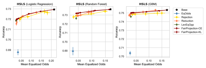
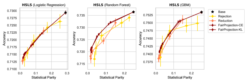
Refer to caption


Figure 3: Accuracy-fairness curves of FairProjection and benchmark methods on the HSLS dataset with 3 different models (Logistic regression, Random forest, GBM). The fairness constraint is MEO.

Refer to caption

Figure 4: Accuracy-fairness curves of FairProjection and benchmark methods on the HSLS dataset with 3 different models (Logistic regression, Random forest, GBM). The fairness constraint is statistical parity.

Refer to caption

Figure 5: Accuracy-fairness curves of FairProjection and benchmark methods on the ENEM-50k-2C dataset with 3 different models (Logistic regression, Random forest, GBM). The fairness constraint is MEO.

Refer to caption


Figure 6: Accuracy-fairness curves of FairProjection and benchmark methods on the ENEM-50k-2C dataset with 3 different models (Logistic regression, Random forest, GBM). The fairness constraint is statistical parity.

Refer to caption

Figure 7: Accuracy-fairness curves of FairProjection and benchmark methods on COMPAS with 3 different models (Logistic regression, Random forest, GBM). The fairness constraint is MEO.

Refer to caption

Figure 8: Accuracy-fairness curves of FairProjection and benchmark methods on COMPAS with 3 different models (Logistic regression, Random forest, GBM). The fairness constraint is statistical parity.

Refer to caption

Figure 9: Accuracy-fairness curves of FairProjection and benchmark methods on the Adult dataset with 3 different models (Logistic regression, Random forest, GBM). The fairness constraint is MEO.

Refer to caption

Figure 10: Accuracy-fairness curves of FairProjection and benchmark methods on the Adult dataset with 3 different models (Logistic regression, Random forest, GBM). The fairness constraint is statistical parity.

Refer to caption

Figure 11: Accuracy-fairness curves of FairProjection-CE and FairProjection-KL on ENEM-50k with with 5 labels, 5 groups and different base classifiers base classifiers. The fairness constraint is MEO.

Refer to caption

Figure 12: Accuracy-fairness curves of FairProjection-CE and FairProjection-KL on ENEM-50k with with 5 labels, 5 groups and different base classifiers base classifiers. The fairness constraint is SP.

Refer to caption

Figure 13: Accuracy-fairness curves of FairProjection-CE and FairProjection-KL on ENEM-50k with with 2 labels, 5 groups and different base classifiers base classifiers. The fairness constraint is MEO.

Refer to caption

Figure 14: Accuracy-fairness curves of FairProjection-CE and FairProjection-KL on ENEM-50k with with 2 labels, 5 groups and different base classifiers base classifiers. The fairness constraint is SP.

Refer to caption

Figure 15: Comparison of FairProjection-CE and FairProjection-KL with Adversarial on ENEM-50k-5-2, meaning 5 labels, 2 groups. The reason for the difference comparing to Fig. 2 is that we resampled 50k data points from ENEM.

B.4 More on related work

Method Feature
Multiclass Multigroup Scores Curve Parallel Rate Metric
Reductions [5] SP, (M)EO
Reject-option [44] SP, (M)EO
EqOdds [35] EO
LevEqOpp [13] FNR
CalEqOdds [50] MEO
FACT [42] SP, (M)EO
Identifying [39] superscript\text{{\color[rgb]{0,0.88,0}{\char 33\relax}}}^{\text{{\color[rgb]{0.72,0,0}{\char 35\relax}}}} SP, (M)EO
FST [53, 54] SP, (M)EO
Overlapping [55] SP, (M)EO
Adversarial [57] N/A SP, (M)EO
FairProjection (ours) SP, (M)EO
Copy of Table 1. Comparison between benchmark methods. Multiclass/multigroup: implementation takes datasets with multiclass/multigroup labels; Scores: processes raw outputs of probabilistic classifiers; Curve: outputs fairness-accuracy tradeoff curves (instead of a single point); Parallel: parallel implementation (e.g., on GPU) is available; Rate: convergence rate or sample complexity guarantee is proved. Metric: applicable fairness metric, with SP\leftrightarrowStatistical Parity, EO\leftrightarrowEqualized Odds, MEO\leftrightarrowMean EO.

Our method is a model-agnostic post-processing method, so we focus our comparison on such post-processing fairness intervention methods. In the above table, the only exception is Adversarial [57], which we use to benchmark multi-class prediction. Adversarial [57] is an in-processing method based on generative-adversarial network (GAN) where the adversary tries to guess the sensitive group attribute S𝑆S from Y𝑌Y and Y^^𝑌\widehat{Y}. Even though this GAN-based approach is applicable to multi-class, multi-group prediction, it cannot be universally applied to any pre-trained classifier like our method.

EqOdds [35], CalEqOdds [50] and LevEqOpp [13] are post-processing methods designed for binary prediction with binary groups. They find different decision thresholds for each group that equalize FNR and FPR of two groups. CalEqOdds [50] has an additional constraint that the post-processed classifier must be well-calibrated, and we observe in our experiments that this stringent constraint leads to a low-accuracy classifier especially when there is a big gap in the base rate between the two groups. FACT [42] follows a similar approach but generalizes this to an optimization framework that can have both equalized odds and statistical parity constraints and flexible accuracy-fairness trade-off. The optimization formulation finds a desired confusion matrix, and their proposed post-processing method flips the predictions to match the desired confusion matrix. Reject-option [44] is similar in that it flips predictions near the decision threshold. In [44], instead of finding the optimal confusion matrix, it performs grid search to find the optimal margin around the decision threshold that can minimize either equalized odds or statistical parity. For these methods that center around modifying decision thresholds, it is not straightforward to extend to multi-class and multi-group as one will have to consider (|𝒴|2)(|𝒮|2)binomial𝒴2binomial𝒮2\binom{|\mathcal{Y}|}{2}\cdot\binom{|\mathcal{S}|}{2} boundaries.

FST [53, 54] tackles fairness intervention via minimizing cross-entropy for binary classes. Their method is inherently tailored to binary classification and only a cross-entropy objective function, and our FairProjection-CE reduces to FST for the case of CE and binary classification tasks. Identifying [39] is a method for minimizing KL-divergence for group-fairness intervention, which changes the label weights (via a convex combination) between unweighted and weighted samples, but it is not clear that this would navigate a good fairness-accuracy trade-off curve. Their method can be extended to non-binary prediction with non-binary groups by an appropriate choice of base classifier and fairness constraints, which is a non-trivial extension of the accompanying code, and we chose not to pursue this. Note that [39] and FairProjection solve the KL-divergence minimization in very different ways. In particular, the runtime of [53, 54] on  350k train is longer than 30 minutes using logistic regression as a base classifier (in comparison, the runtime of FairProjection for a 500k dataset is less than 1 minute). This is because they require reweighing the data and retraining a large number of times. Hence, it is inherently non-parallelizable.

B.4.1 Fairness in Multi-Class Prediction

Methods that are based on optimization with a fairness regularizer often can be easily extended to multi-class prediction as it only requires a small change in the regularizer. For example, instead of using |FNR0(x)FNR1(x)|subscriptFNR0𝑥subscriptFNR1𝑥|\text{FNR}_{0}(x)-\text{FNR}_{1}(x)|, one can replace this with

i𝒴ji𝒴|P(Y^=jY=i,S=0)P(Y^=jY=i,S=1)|.\sum_{i\in\mathcal{Y}}\sum_{j\neq i\in\mathcal{Y}}|P(\widehat{Y}=j\mid Y=i,S=0)-P(\widehat{Y}=j\mid Y=i,S=1)|. (119)

FERM [27] mentions how their method can be extended to multi-class sensitive attribute. Similarly, we believe that their method can be used for multi-class labels as well. The reductions approach [5] assumes binary labels but is has natural extension to multi-class, which is explored in [55]. In-processing methods proposed in [17] and [57] allow for both multi-class labels and multi-class group attributes. [57] aims to achieve the independence between the sensitive attribute S𝑆S and Y^^𝑌\widehat{Y} or Y^^𝑌\widehat{Y} given Y𝑌Y by training an adversary who tries to figure out S^^𝑆\widehat{S}. [17] directly estimates the fairness loss (e.g., 119) using kernel density estimation. They also demonstrate the empirical performance in a three-class classification using synthetic data. Another in-processing method is [2] where the authors propose a way to incorporate multi-class fairness constraints into decision tree training. The preprocessing method suggested in [19] is conceptually similar to our methods in that it aims to minimize the KL-divergence between the original distribution and preprcoessed distribution while satisfying fairness constraints. Their method, however, requires all feature vectors to be binary, and applies only to demographic parity or representation rate. There exist other notions of fairness, which is different from commonly-used group fairness metrics such as envy-freeness [9] or best-effort [43], which can be applied to multi-class prediction tasks.

Finally, there are unpublished works [24, 56] that could handle multi-class classification. Specifically, [24] presents a post-processing method that selects different thresholds for each group to achieve demographic parity. [56] formulates SVM training as a mixed-integer program and integrates fairness regularizer in the objective, which can also deal with multi-class.

Appendix C Datasheet for ENEM 2020 dataset

Questions

The questions below are derived from [33] and aim to provide context about the ENEM-2020 dataset. We highlight that we did not create the dataset nor collect the data included in it. Instead, we simply provide a link to the ENEM-2020 data at [37]. At the time of writing, the ENEM-2020 dataset is open and made freely available by the Brazilian Government at [37] under a Creative Commons Attribution-NoDerivs 3.0 Unported License [20]. We provide the datasheet below to clarify certain aspects of the dataset (e.g., motivation, composition, etc.) since the original information is available in Portuguese at [37], thus limiting its access to a broader audience. The website [37] contains a link to download a .zip file which contains the ENEM-2020 data in .csv format and extensive accompanying documentation.

The datasheet below is not a substitute for the explanatory files that are downloaded together with the dataset at [37], and we emphatically recommend the user to familiarize themselves with associated documentation prior to usage. We also strongly recommend the user to carefully read the “Leia-Me” (readme) file Leia_Me_Enem_2020.pdf available in the same .zip folder that contains the dataset. The answers in the datasheet below are based on an English translation of information available at [37] and may be incomplete or inaccurate. The datasheet below is based on our own independent analysis and in no way represents or attempts to represent the opinion or official position of the Brazilian Government and its agencies.

We also note that we do not distribute the ENEM-2020 dataset directly nor host the dataset ourselves. Instead, we provide a link to download the data from a public website hosted by the Brazilian Government. The dataset may become unavailable in case the link in [37] becomes inaccessible.

Motivation

  • For what purpose was the dataset created? According to the “Leia-me” (Read Me) file that accompanies the data, the dataset was made available to fufill the mission of the Instituto Nacional de Estudos e Pesquisas Educacionais Anísio Teixeira (INEP) of developing and disseminating data about exams and evaluations of basic education in Brazil.

  • Who created the dataset (e.g., which team, research group) and on behalf of which entity (e.g., company, institution, organization)? The dataset was developed by INEP, which is a government agency connected to the Brazilian Ministry of Education.

  • Who funded the creation of the dataset? The data is made freely available by the Brazilian Government.

Composition

  • What do the instances that comprise the dataset represent (e.g., documents, photos, people, countries)? The instances of the dataset are information about individual students who took the Exame Nacional do Ensino Médio (ENEM). The ENEM is the capstone exam for Brazilian students who are graduating or have graduated high school.

  • How many instances are there in total (of each type, if appropriate)? The raw data provided in at [37] has approximately 5.78 million entries. The processed version we use in our experiments has approximately 1.4 million entries.

  • Does the dataset contain all possible instances or is it a sample (not necessarily random) of instances from a larger set? The data provided is the lowest level of aggregation of data collected from ENEM exam-takers made available by INEP.

  • What data does each instance consist of? We provide a brief description of the features available in the raw public data provided at [37]. Upon downloading the data, a detailed description of features and their values are available (in Portuguese) in the file titled Dicionário_Mircrodados_ENEM_2020.xsls. The features include:

    • Information about exam taker: exam registration number (masked), year the exam was taken (2020), age range, sex, marriage status, race, nationality, status of high school graduation, year of high school graduation, type of high school (public, private, n/a), if they are a “treineiro” (i.e., taking the exam as practice).

    • School data: city and state of participant’s school, school administration type (private, city, state, or federal), location (urban or rural), and school operation status.

    • Location where exam was taken: city and state.

    • Data on multiple-choice questions: The exam is divided in 4 parts (translated from Portuguese): natural sciences, human sciences, languages and codes, and mathematics. For each part there is data if the participant attended the corresponding portion of the exam, the type of exam book they received, their overall grade, answers to exam questions, and the answer sheet for the exam.

    • Data on essay question: if participant took the exam, grade on different evaluation criteria, and overall grade.

    • Data on socio-economic questionnaire answers: the data include answers to 25 socio-economic questions (e.g., number of people who live in your house, family average income, if the your house has a bathroom, etc.).

  • Is there a label or target associated with each instance? No, there is no explicit label. In our fairness benchmarks, we use grades in various components of the exam as a predicted label.

  • Is any information missing from individual instances? Yes, certain instances have missing values.

  • Are relationships between individual instances made explicit (e.g., users’ movie ratings, social network links)? No explicit relationships identified.

  • Are there recommended data splits (e.g., training, development/validation, testing)? No.

  • Are there any errors, sources of noise, or redundancies in the dataset? The data contains missing values and, according to INEP, was collected from individual exam takers. The information is self-reported and collected at the time of the exam.

  • Is the dataset self-contained, or does it link to or otherwise rely on external resources (e.g., websites, tweets, other datasets)? Self-contained.

  • Does the dataset contain data that might be considered confidential (e.g., data that is protected by legal privilege or by doctor–patient confidentiality, data that includes the content of individuals’ non-public communications)? According to the Leia-me (readme) file (in Portuguese) that accompanies the dataset and our own inspection, the dataset does not contain any feature that allows direct identification of exam takers such as name, email, ID number, birth date, address, etc. The exam registration number has been substituted by a sequentially generated mask. INEP states that the released data is aligned with the Brazilian Lei Geral de Proteção dos Dados (LGPD, General Law for Data Protection). We emphatically recommend the user to view the Readme file prior to usage.

  • Does the dataset contain data that, if viewed directly, might be offensive, insulting, threatening, or might otherwise cause anxiety? The official terminology used by the Brazilian Government to denote race can be viewed as offensive. Specifically, the term used to describe the race of exam takers of Asian heritage is “Amarela,” which is the Portuguese word for the color yellow. Moreover, the term “Pardo,” which roughly translates to brown, is used to denote individuals of multiple or mixed ethnicity. This outdated and inappropriate terminology is still in official use by the Brazilian Government, including in its population census. The dataset itself includes integers to denote race, which are mapped to specific categories through the variable dictionary.

  • Does the dataset relate to people? Yes.

  • Does the dataset identify any subpopulations (e.g., by age, gender)? Yes. Information about age, sex, and race are included in the dataset.

  • Is it possible to identify individuals (i.e., one or more natural persons), either directly or indirectly (i.e., in combination with other data) from the dataset? The Leia-me (readme) file notes that the individual exam-takers cannot be directly identified from the data. However, in the same file, INEP recognizes that the Brazilian data protection law (LGPD) does not clearly define what constitutes a reasonable effort of de-identification. Thus, INEP adopted a cautious approach: this dataset is a simplified/abbreviated version of the ENEM micro-data compared to prior releases and aims to remove any features that may allow identification of the exam-taker.

  • Does the dataset contain data that might be considered sensitive in any way (e.g., data that reveals racial or ethnic origins, sexual orientations, religious beliefs, political opinions or union memberships, or locations; financial or health data; biometric or genetic data; forms of government identification, such as social security numbers; criminal history)? The data includes race information and socio-economic questionnaire answers.

Collection Process

Since we did not produce the data, we cannot speak directly about the collection process. Our understanding is that the data contains self-reported answers from exam-takers of the ENEM collected at the time of the exam. The exam was applied on 17 and 24 of January 2021 (delayed due to COVID). The data was aggregated and made publicly available by INEP at [37]. After consulting the IRB office at our institution, no specific IRB was required to use this data since it is anonymized and publicly available.

Preprocessing/cleaning/labeling

  • Was any preprocessing/cleaning/labeling of the data done (e.g., discretization or bucketing, tokenization, part-of-speech tagging, SIFT feature extraction, removal of instances, processing of missing values)? Some mild pre-processing was done on the data to ensure anonymity, as indicated in the “Leia-me” file. This includes aggregating participant ages, masking exam registration numbers, and removing additional information that could allow de-anonymization.

  • Was the “raw” data saved in addition to the preprocessed/cleaned/labeled data (e.g., to support unanticipated future uses)? The raw data is not publicly available.

Uses

  • Has the dataset been used for any tasks already? We have used this dataset to benchmark fairness interventions in ML in the present paper. ENEM microdata has also been widely used in studies ranging from public policy in Brazil to item response theory in high school exams.

  • Are there tasks for which the dataset should not be used? INEP does not clearly define tasks that should not be used on this dataset. However, no attempt should be made to de-anonymize the data.

Distribution and Maintenance

The ENEM-2020 dataset is open and made freely available by the Brazilian Government at [37] under a Creative Commons Attribution-NoDerivs 3.0 Unported License [20] at the time of writing. The dataset may become unavailable in case the link in [37] becomes inaccessible.