Cosmological constraints from the power spectrum and bispectrum of 21cm intensity maps

Abstract

The 21cm emission of neutral hydrogen is a potential probe of the matter distribution in the Universe after reionisation. Cosmological surveys of this line intensity will be conducted in the coming years by the SKAO and HIRAX experiments, complementary to upcoming galaxy surveys. We present the first forecasts of the cosmological constraints from the combination of the 21cm power spectrum and bispectrum. Fisher forecasts are computed for the constraining power of these surveys on cosmological parameters, the BAO distance functions and the growth function. We also estimate the constraining power on dynamical dark energy and modified gravity. Finally we investigate the constraints on the 21cm clustering bias, up to second order. We take into account the effects on the 21cm correlators of the telescope beam, instrumental noise and foreground avoidance, as well as the Alcock-Paczynski effect and the effects of theoretical errors in the modelling of the correlators. We find that, together with Planck priors, and marginalising over clustering bias and nuisance parameters, HIRAX achieves sub-percent precision on the $\Lambda$CDM parameters, with SKAO delivering slightly lower precision. The modified gravity parameter $\gamma$ is constrained at 1% (HIRAX) and 5% (SKAO). For the dark energy parameters $w_{0},w_{a}$, HIRAX delivers percent-level precision while SKAO constraints are weaker. HIRAX achieves sub-percent precision on the BAO distance functions $D_{A},H$, while SKAO reaches $1-2\%$ for $0.6\lesssim z\lesssim 1$. The growth rate $f$ is constrained at a few-percent level for the whole redshift range of HIRAX and for $0.6\lesssim z\lesssim 1$ by SKAO. The different performances arise mainly since HIRAX is a packed inteferometer that is optimised for BAO measurements, while SKAO is not optimised for interferometer cosmology and operates better in single-dish mode, where the telescope beam limits access to the smaller scales that are covered by an interferometer.

1 Introduction

The tightest constraints on cosmological parameters have been provided by cosmic microwave background (CMB) anisotropies as measured by Planck [1] and by large-scale structure (LSS) surveys such as SDSS and DES. Next-generation LSS surveys with DESI [2], Euclid [3], LSST [4], SKAO [5] and HIRAX [6], combined with CMB data, will significantly improve over the current measurements.

The post-reionisation 21cm emission line of neutral hydrogen (HI) is a tracer of the underlying matter distribution. Detecting individual 21cm-emitting galaxies is a difficult task, especially at higher redshifts, given the weakness of the line. If instead we measure the integrated emission in each pixel, we can perform large-volume surveys of the HI fluctuations – known as 21cm (equivalently, HI) intensity mapping surveys [7]. Such spectroscopic surveys are planned with SKAO-MID (hereafter referred to as SKAO) and HIRAX, which we consider here. They will provide an exciting and important complementary probe to the traditional optical/ infra-red LSS surveys, with completely different systematics. In addition to their wide sky areas, these surveys will together cover the redshift range $0<z\lesssim 3$, beyond the range accessed by cosmological galaxy surveys.

Cosmological constraints are typically performed using the power spectrum. The addition of the bispectrum is known to improve constraining power (to varying degrees) and to break parameter degeneracies, as has been shown in recent work on BOSS galaxy surveys [8, 9, 10, 11]. (For recent work on the galaxy bispectrum, see e.g. [12, 13, 14, 15, 16].) Regarding 21cm intensity mapping, the combination of the power spectrum and bispectrum has been used to investigate future constraints on primordial non-Gaussianity [17, 18]. Here we use the same combination to forecast constraints from 21cm intensity mapping surveys on standard cosmological parameters, dark energy parameters and a modified gravity parameter. We also derive constraints on redshift-dependent BAO (baryon acoustic oscillation) distances and on the growth rate function.

In contrast to galaxy surveys, HI intensity mapping is contaminated by huge foregrounds, similar to the CMB. Within the simplified framework of Fisher forecasting, we follow the usual approach of foreground avoidance (e.g. [19, 17]), since foreground cleaning requires substantial numerical simulations (e.g. [20]). Another difference lies in the noise: for HI intensity mapping on linear/ quasi-linear scales, the shot noise can be neglected since it is dominated by instrumental noise. Apart from these two differences we apply a fairly standard analysis, based on the tree-level power spectrum and bispectrum, but with modifications to incorporate nonlinear redshift-space distortions, which affect smaller scales than the tree-level limit. We also apply ‘theoretical errors’ to the covariances in order to take account of inaccuracies in the modeling. In our Fisher analysis, we marginalise over all nuisance parameters.

Our overall finding is that the upcoming HI intensity mapping surveys can deliver exquisite precision on the cosmological parameters and functions, as well as on the clustering bias parameters, with HIRAX out-performing SKAO, based on the different designs of the two surveys.

The remainder of the paper is organised as follows. Section 2 presents the theoretical analysis of the redshift-space power spectrum and bispectrum, including the clustering biases and the Alcock-Paczynski (AP) effect. Details of the HI intensity mapping surveys are presented in Section 3, including the telescope specifications, the associated instrumental noise and the effect of the telescope beam. We make clear the differences between interferometer surveys (HIRAX and its precursor) and single-dish surveys (SKAO and its precursor). In Section 4 we discuss in some detail the Fisher analysis and the various parameters that are included with the relevant priors. The theoretical error contribution to the covariances is also summarised. Our results are presented in Section 5, in the form of tables, contour plots and plots of redshift-dependent errors. We also interpret these results and comment on the differences between the interferometer and single-dish surveys. Finally, Section 6 summarises our main results.

2 Theoretical Model

The HI power spectrum and bispectrum in redshift space will be modelled perturbatively by using the Standard Perturbation Theory (SPT), which assumes that the dynamics of long-wavelength density and velocity perturbations are driven by the hydrodynamics of an Eulerian pressureless perfect fluid (see [21] for a review). Moreover, a complete bias and redshift space distortions (RSD) expansion, up to the lowest non-vanishing order in the perturbations, will be considered. A phenomenological non-perturbative description will be used for the so-called fingers-of-God effect (FoG) [22], caused by the virialized motions of galaxies, which cannot be described within the framework of SPT. Gaussian initial conditions will be considered throughout this work, while the analysis will be restricted within the linear/semi-linear regime, where the tree-level power spectrum and bispectrum provide an adequate description.

2.1 Matter power spectrum and bispectrum

The power spectrum of the Bardeen gauge-invariant primordial gravitational potential is defined in Fourier space by

$$\langle\Phi(\bm{k})\Phi(\bm{k}^{\prime})\rangle=(2\pi)^{3}\delta_{\rm D}(\bm{k}+\bm{k}^{\prime})P_{\Phi}(k),$$ (2.1)

where $P_{\Phi}(k)$ is related to the power spectrum of the primordial curvature perturbations, generated during inflation. For the standard single-field slow-roll inflationary scenario, their distribution should be nearly perfect Gaussian. The primordial perturbations $\Phi$ are in turn related to the linear dark matter density contrast through the Poisson equation, $\delta_{\rm m}^{\rm L}(\bm{k},z)=M(k,z)\Phi(\bm{k})$, where

$$M(k,z) = \frac{2c^{2}D(z)}{3\Omega_{\rm m}H_{0}^{2}\,}\,T(k)\,k^{2}.$$ (2.2)

Here $D(z)$ is the growth factor of the linearly evolved density contrast, normalised to unity today (i. ​e. $D(0)=1$), and $T(k)$ is the matter transfer function normalized to unity at large scales, $k\rightarrow 0$. The linear matter power spectrum ($P_{\rm m}^{L}(k,z)=M^{2}(k,z)P_{\Phi}(k)$) will be computed with the numerical Boltzmann code CAMB [23].

For Gaussian initial conditions, higher-order correlators are non-zero due to the non-linearities induced by gravity. The most important is the bispectrum, i. ​e. the Fourier transform of the three-point function:

$$\langle\delta_{\rm m}(\bm{k}_{1})\delta_{\rm m}(\bm{k}_{2})\delta_{\rm m}(\bm{k}_{3})\rangle=(2\pi)^{3}\delta_{\rm D}(\bm{k}_{1}+\bm{k}_{2}+\bm{k}_{3})B_{\rm m}(k_{1},k_{2},k_{3}).$$ (2.3)

Here the Dirac delta function ensures the conservation of momentum.

The fiducial cosmology is given by the average values of the flat $\Lambda$CDM model, measured by the Planck mission. In particular we use the base_plikHM_TTTEEE_lowl_lowE_lensing column of the Planck 2018 results [1].

2.2 Neutral hydrogen bias

Cosmological forecasting from future HI IM surveys (see Section 3 for details) requires a robust description of the relation between the statistics of observed tracers and the underlying distribution of dark matter, i. ​e. the clustering bias.

The density contrast of halos $\delta_{\rm h}$ can be expressed perturbatively as a series of operators, constructed out of all possible local gravitational observables [24, 25, 26] (i. ​e. operators formed by the tidal tensor $\partial_{i}\partial_{j}\Phi$ and its derivatives, where $\Phi$ can be the Newtonian gravitational potential or the velocity potential $\Phi_{\upsilon}$), satisfying rotational symmetry and the equivalence principle (see e.g. [27] for a review). For Gaussian initial conditions and the spacial scales considered here, the complete set of terms up to second order is needed. The Eulerian halo density overdensity can be written as

$$\delta_{\rm h}^{\rm E}(\bm{x},\tau)=b_{1}^{\rm E}(\tau)\delta_{\rm m}(\bm{x},\tau)+\varepsilon^{\rm E}(\bm{x},\tau)+\frac{b_{2}^{\rm E}(\tau)}{2}\delta_{\rm m}^{2}(\bm{x},\tau)+\frac{b_{s^{2}}^{\rm E}(\tau)}{2}s^{2}(\bm{x},\tau)+\varepsilon_{\delta}^{\rm E}(\bm{x},\tau)\delta_{\rm m}(\bm{x},\tau)\,,$$ (2.4)

where $\tau$ is conformal time, $\bm{x}$ are spatial comoving coordinates in the Eulerian frame, $s^{2}=s_{ij}s^{ij}$ is the simplest scalar that can be formed from the tidal field, $\varepsilon^{\rm E}$ is the leading stochastic field [28, 29, 30] and $\varepsilon_{\delta}^{\rm E}$ is the stochastic field associated with the linear bias. These fields take into account the stochastic relation between the galaxy density and any large-scale field. The higher-order derivative term, which encapsulates short-scale dynamics and is present at second-order, is excluded from the expansion since the spacial scales considered here are much larger than the Langrangian radius of halos hosting the galaxies of interest.

Applying the general bias expansion, described before, to the neutral hydrogen, an additional ingredient is needed, namely the description on how HI is distributed within the dark matter halos. This can be achieved within the framework of the halo model [31, 32, 33]. In this approach, HI is assumed to occupy regions within the halos, with a negligible contribution outside of them. The HI density is then defined as [34, 35]:

$$\rho_{\rm HI}(z)=\int{\rm d}M\,n_{\rm h}(M,z)M_{\rm HI}(M,z),$$ (2.5)

where $M_{\rm HI}$ is the average HI mass within the halo of total mass $M$ at redshift $z$. The halo mass function, $n_{\rm h}(M,z)$, is considered to be the best-fit results of [36], which originate from fitting to N-body simulations. For $M_{\rm HI}$ we use a halo occupation distribution (HOD) approach [37] and follow the model of [35]:

$$M_{\rm HI}(M,z)=C(z)(1-Y_{p})\frac{\Omega_{\rm b}}{\Omega_{\rm m}}\,{\rm e}^{-M_{\rm min}(z)/M}\,M^{q(z)},$$ (2.6)

where $C$ is a normalization constant, $Y_{p}=0.24$ is the helium fraction, $M_{\rm min}$ is the halo mass below which the amount of HI in halos is exponentially suppressed, and $q$ controls the efficiency of generating or destroying neutral hydrogen inside halos. The power-law is in agreement with the numerical results from hydrodynamic simulations of [38, 39], while the presence of the exponential cut-off ensures the suppression of HI in low-mass halos [40, 41, 34]. The fiducial values of the HOD free parameters are ${q}=1$ and $M_{\rm min}=5\times 10^{9}M_{\odot}/h$.

The HI bias coefficients are given by

$$b_{\rm HI}^{i}(z)=\frac{1}{\rho_{\rm HI}(z)}\int_{0}^{\infty}{\rm d}M\,n_{\rm h}(M,z)b_{i}^{\rm h}(M,z)M_{\rm HI}(M,z),$$ (2.7)

where the index $i$ corresponds to the subscripts of the bias terms in the expansion of Equation 2.4. For the linear halo bias we use the the fitting function of [42], while for the quadratic bias the analytic expression is derived after using the mass function of [36] and the peak-background split argument [43, 17]. In [43] it is shown that both expressions are in good agreement with numerical results for the HI mass ranges considered here. The second-order tidal field bias coefficient is related to the linear bias by $b_{s^{2}}^{\rm E}=-4(b_{1}^{\rm E}-1)/7$ [44].

2.3 Power spectrum and bispectrum in redshift space

The distance of a luminous object is determined by its motion with the Hubble flow, which is affected by its peculiar velocity. This effect is known as a redshift space distortion [45, 46, 47] and can be taken into account by mapping the real space correlator to redshift space. Here we will consider the flat-sky approximation, i. ​e. the line-of-sight vector $\hat{\bm{z}}$ is a constant unit vector. In the non-perturbative regime, the velocity dispersion of objects during the virialisation process make structures appear more elongated along the line of sight, compared to real space, i. ​e. the FoG effect. It is treated here phenomenologically, by introducing an exponential damping factor, which models the suppression of clustering power in redshift space.

The tree-level expressions for the HI power spectrum and bispectrum in redshift space are given by:

$$P_{\rm HI}(\bm{k},z) =\bar{T}(z)^{2}\Big{[}D_{\text{FoG}}^{P}(\bm{k},z)Z_{1}(\bm{k},z)^{2}P_{\rm m}(k,z)+P_{\varepsilon}(z)\Big{]}+P_{\rm N}(\bm{k},z),$$ (2.8)

$$B_{\rm HI}(\bm{k}_{1},\bm{k}_{2},\bm{k}_{3},z) =\bar{T}(z)^{3}\bigg{\{}D_{\text{FoG}}^{B}(\bm{k}_{1},\bm{k}_{2},\bm{k}_{3},z)$$

$$\leavevmode\nobreak\ \times\bigg{[}2Z_{1}(\bm{k}_{1},z)Z_{1}(\bm{k}_{2},z)Z_{2}(\bm{k}_{1},\bm{k}_{2},z)P_{\rm m}^{\rm L}(k_{1},z)P_{\rm m}^{\rm L}(k_{2},z)+2\leavevmode\nobreak\ \text{perm}\bigg{]}$$

$$\leavevmode\nobreak\ +2P_{\varepsilon\varepsilon_{\delta}}(z)\Big{[}Z_{1}(\bm{k}_{1},z)P_{\rm m}^{\rm L}(k_{1},z)+2\leavevmode\nobreak\ \text{perm}\Big{]}+B_{\varepsilon}(z)\bigg{\}}.$$ (2.9)

In HI IM, $P_{\rm N}$ is the instrumental noise (see Section 3), where it is assumed to be Gaussian (see [19] for a discussion) and therefore it is only present in the two-point correlator. The background temperature is $\bar{T}=188\,\Omega_{\rm HI}(z)h(1+z)^{2}H_{0}/H(z)\leavevmode\nobreak\ \mu$K, where the cosmic evolution of the HI density is modelled as $\Omega_{\rm HI}(z)=4\times 10^{-4}(1+z)^{0.6}$ [48]. The general redshift kernels up to second order and for Gaussian initial conditions are:

$$Z_{1}(\bm{k}_{i})=b_{1}+f\mu_{i}^{2},$$ (2.10)

$$Z_{2}(\bm{k}_{i},\bm{k}_{j})=b_{1}F_{2}(\bm{k}_{i},\bm{k}_{j})+f\mu_{ij}^{2}G_{2}(\bm{k}_{i},\bm{k}_{j})+\frac{b_{2}}{2}+\frac{b_{s^{2}}}{2}S_{2}(\bm{k}_{i},\bm{k}_{j})$$

$$+\frac{1}{2}f\mu_{ij}k_{ij}\left[\frac{\mu_{i}}{k_{i}}Z_{1}(\bm{k}_{j})+\frac{\mu_{j}}{k_{j}}Z_{1}(\bm{k}_{i})\right],$$ (2.11)

where $f$ is the linear growth rate, $\mu_{i}=\hat{\bm{k}}_{i}\cdot\hat{\bm{z}}$, $\mu_{ij}=(\mu_{i}k_{i}+\mu_{j}k_{j})/k_{ij}$ and $k_{ij}^{2}=(\bm{k}_{i}+\bm{k}_{j})^{2}$. Note that we suppressed the redshift dependence for brevity. The kernels $F_{2}(\bm{k}_{i},\bm{k}_{j})$ and $G_{2}(\bm{k}_{i},\bm{k}_{j})$ are the second-order symmetric SPT kernels [21], while $S_{2}(\bm{k}_{1},\bm{k}_{2})=(\hat{\bm{k}}_{1}\cdot\hat{\bm{k}}_{2})^{2}-1/3$ is the tidal kernel [49, 44]. The FoG damping factors are [50, 51]

$$D_{\text{FoG}}^{P}(\bm{k},z) =\exp\big{[}-k^{2}\mu^{2}\,\sigma_{P}(z)^{2}\big{]},$$ (2.12)

$$D_{\text{FoG}}^{B}(\bm{k}_{1},\bm{k}_{2},\bm{k}_{3},z) =\exp\big{[}-\big{(}k_{1}^{2}\mu_{1}^{2}+k_{2}^{2}\mu_{2}^{2}+k_{3}^{2}\mu_{3}^{2}\big{)}\sigma_{B}(z)^{2}\big{]},$$ (2.13)

where the damping parameters $\sigma_{P}$ and $\sigma_{B}$ have fiducial value equal to the linear velocity dispersion $\sigma_{\upsilon}$. The stochastic terms (i. ​e. $P_{\varepsilon}$, $P_{\varepsilon\varepsilon_{\delta}}$ and $B_{\varepsilon}$) approach their asymptotic constant values as $k\rightarrow 0$. For the scales considered here, the Poisson distribution characterises fully the correlation of these components, hence these predictions will be used as fiducial values for the shot-noise contributions. In the HI halo model formalism (Section 2.2), the shot noise term is given by [35]

$$P_{\rm SN}(z)=\frac{1}{\overline{n}_{\rm eff}(z)}=\frac{1}{\rho_{\rm HI}(z)}\int{\rm d}\ln M\,n_{\rm h}(M,z)M_{\rm HI}^{2}.$$ (2.14)

The effective number density can in turn be used for the fiducial values of all the stochastic contributions [52, 27]:

$$P_{\varepsilon}\equiv P_{\rm SN},\quad P_{\varepsilon\varepsilon_{\delta}}=\frac{b_{1}}{2\overline{n}_{\rm eff}},\quad B_{\varepsilon}=\frac{1}{\overline{n}_{\rm eff}^{2}}.$$ (2.15)

The redshift-space bispectrum is characterized by five variables: three to define the triangle shape (e.g. the sides $k_{1}$, $k_{2}$, $k_{3}$) and two to characterize the orientation of the triangle relative to the line of sight. The angles characterising this orientation are, following [53], the polar angle $\theta$ of $\bm{k}_{1}$, with $\cos\theta=\mu\equiv\hat{\bm{k}}_{1}\cdot\hat{\bm{z}}$ and the azimuthal angle $\phi$ around $\bm{k}_{1}$. Then the cosines of the angles that the wave-vectors make with the line of sight are: $\mu_{1}=\mu$, $\mu_{2}=\mu\cos x_{12}+\sqrt{1-\mu^{2}}\sin x_{12}\sin\phi$ and $\mu_{3}=-(k_{1}/k_{3})\mu_{1}-(k_{2}/k_{3})\mu_{2}$, where $\cos x_{12}=\hat{\bm{k}}_{1}\cdot\hat{\bm{k}}_{2}$. Then $B_{\rm HI}(\bm{k}_{1},\bm{k}_{2},\bm{k}_{3},z)=B_{\rm HI}(k_{1},k_{2},k_{3},\mu_{1},\phi,z)$. Here we focus on the monopole of the tree-level bispectrum, obtained after taking the average over all directions. In [54], it is shown that the lowest-order bispectrum multipoles do not suffer from a significant loss of information on most of the cosmological parameters and bias coefficients (see also [55] for a discussion).

In this work we stay mostly within the perturbative regime, slightly venturing into mildly nonlinear scales for low redshift. For the power spectrum, the tree-level description is sufficient. Nonetheless, in order to improve the precision of the matter modelling, instead of using the linear power spectrum $P^{\rm L}_{\rm m}$ to describe $P_{\rm m}$ in Equation 2.8, we use the non-linear matter power spectrum, $P^{\rm NL}_{\rm m}$, from the updated version of the HMCode augmented halo model [56]. The HMCode approach provides more accurate predictions, over a large range of scales, relative to the usual Halofit model [57, 58], as shown in [59, 56]. In addition, a general feature of the Halofit approach is the poor performance in predicting the derivatives of the power spectrum with respect to some cosmological parameters [60]. This indicates that the usage of Halofit, in a Fisher matrix error forecast, hides inaccuracies and should be used with extreme caution. In order to avoid the possibility of unreliable Fisher information matrix calculation, we use the HMCode, evaluated with the latest version of CAMB, to describe the non-linear matter power spectrum.

For the bispectrum, the tree-level modelling provides an adequate description for the high-order clustering of HI on the scales considered here [61, 62, 63, 64, 65, 66, 67, 8]. Nonetheless, for both correlators, we will take into account the parameter shift due the exclusion of higher-order contributions in the matter and bias expansions, at the Fisher matrix level, through the ‘theoretical errors’ approach (see Section 4.4).

2.4 Alcock-Paczynski effect

Another source of anisotropies in the observed galaxy clustering, in addition to RSD, is the AP effect [68], which occurs when the fiducial cosmology, used to convert the observed angular coordinates and redshifts to physical distances, differs from the true one. This leads to an artificial anisotropic distortion of the inferred galaxy distribution, which modulates the amplitude and shape of the power spectrum and bispectrum. The radial and transverse distortions are proportional to the Hubble parameter $H(z)$ and angular diameter distance $D_{A}(z)$ respectively. This provides additional information on probing the underlying cosmology, and this effect is taken into account in our forecasts.

The AP distortions rescale the radial and transverse components of $\bm{k}$ (fiducial cosmology) as, $q_{\parallel}=k_{\parallel}[H_{\rm true}(z)/H_{\rm fid}(z)]$ and $q_{\bot}=k_{\bot}[D_{A,\rm fid}(z)/D_{A,\rm true}(z)]$, where $\bm{q}$ is the wave-vector in the true cosmology. The relation between the fiducial ($k$, $\mu$) and the true ($q$, $\nu$) is given by:

$$q(k,\mu) =k\alpha(\mu)\;,\quad\nu(k,\mu)=\frac{\mu}{\alpha(\mu)}\frac{H_{\rm true}}{H_{\rm fid}}\;,$$ (2.16)

$$\alpha(\mu) =\left[\left(\frac{H_{\rm true}}{H_{\rm fid}}\right)^{2}\mu^{2}+\left(\frac{D_{A,\rm fid}}{D_{A,\rm true}}\right)^{2}\left(1-\mu^{2}\right)\right]^{1/2},$$ (2.17)

where here and below we suppress the redshift dependence for clarity. The observed power spectrum with AP effect [69] and bispectrum with AP effect [70] are

$$P^{\rm obs}_{\rm HI}\left(k,\mu,z\right) =\left(\frac{H_{\rm true}}{H_{\rm fid}}\right)\left(\frac{D_{A,\rm fid}}{D_{A,\rm true}}\right)^{2}P_{\rm HI}\big{(}q,\nu,z\big{)},$$ (2.18)

$$B^{\rm obs}_{\rm HI}\left(k_{1},k_{2},k_{3},\mu_{1},\phi,z\right) =\left(\frac{H_{\rm true}}{H_{\rm fid}}\right)^{2}\left(\frac{D_{A,\rm fid}}{D_{A,\rm true}}\right)^{4}B_{\rm HI}\left(q_{1},q_{2},q_{3},\nu_{1},\phi,z\right).$$ (2.19)

Note that for the Fisher matrix calculations, only $H_{\rm true}$ and $D_{A,\rm true}$ are varied (i. ​e. free parameters), where their fiducial values are taken to be those that correspond to the fiducial cosmology, while $H_{\rm fid}$ and $D_{A,\rm fid}$ remain fixed.

3 HI intensity mapping surveys

Radio telescopes can probe the Universe in two distinct ways: in interferometer (IF) mode, by correlating the signal from all dishes/dipole stations and outputting directly the Fourier transformation of the sky; or single-dish (SD) mode, by providing separate maps of the sky, which are added together to reduce noise, and the final summed map is then Fourier transformed.

The surveys considered here include current and near-future surveys: MeerKAT, a 64-dish already-operational precursor for SKAO (which will have 64+133 dishes), functioning in SD mode, and HIRAX [6], which will have initially 256 dishes and then 1024, operating in IF mode.

In the case of a line intensity mapping survey the noise component on relevant scales is dominated by the thermal noise from the instrument, while the shot-noise contribution remains minimal [71]. In IF mode, a Gaussian model of instrumental noise is given by [72, 73]

$$P^{\rm IF}_{\rm N}(k_{\bot},{z})=T_{\rm sys}(z)^{2}\chi(z)^{2}\lambda(z)\frac{(1+z)}{H(z)}\left[\frac{\lambda(z)^{2}}{A_{\rm e}}\right]^{2}\frac{1}{2\,n_{\rm b}({u},z)\,t_{\rm{survey}}}\frac{S_{\rm area}}{\theta_{\rm b}(z)^{2}}\,,$$ (3.1)

where $t_{\rm{survey}}$ is the integration time, $S_{\rm area}$ is the survey sky area, and $\lambda(z)=\lambda_{21}(1+z)$ is the observed wavelength of the 21cm line. The field of view of a dish with diameter $D_{\rm dish}$ is $\theta_{\rm b}^{2}$, where $\theta_{\rm b}(z)=1.22\,\lambda(z)/D_{\rm dish}$ is the FWHM of the beam of an individual dish. The effective area $A_{\rm e}=\eta\pi(D_{\rm dish}/2)^{2}$ depends on the efficiency $\eta$; for HIRAX we take $\eta=0.7$. The system temperature $T_{\rm sys}$ is the receiver temperature $T_{\rm rx}=50\,{\rm K}$ for HIRAX plus the sky temperature $T_{\rm sky}$, which is taken from Appendix D of [74]. The survey specifications are presented in Table 1.

The baseline density $n_{\rm b}$ is defined in the image plane, where we assume azimuthal symmetry. At an observed wavelength $\lambda$, the physical baseline corresponding to $u$ is $L=u\lambda$. $n_{\rm b}$ vanishes beyond the maximum baseline. For HIRAX, we take the baseline distributions from simulations of the array, presented in Appendix A.

IF Survey	HIRAX-256	HIRAX-1024
redshift	$0.775-2.55$	$0.775-2.55$
$N_{\rm dish}$	$256$	$1,024$
$D_{\rm dish}$ [m]	$6$	$6$
$D_{\rm max}$ [km]	$0.25$	$0.25$
$S_{\rm area}$ [$\rm{deg}^{2}$]	$15,000$	$15,000$
$t_{\rm survey}$ [hrs]	$17,500$	$17,500$

Table 1: Details for the interferometer-mode surveys with HIRAX (from [6]).

SD Survey	MeerKAT		SKAOa
	L Band	UHF Band	Band 1	Band 2
redshift	0.1${}^{b}-$0.58	0.4${}^{c}-$1.45	0.35${}^{d}-$3.05	0.1${}^{b}-$0.49
$N_{\rm dish}$	$64$	$64$	$197$	$197$
$D_{\rm dish}$ [m]	$13.5$	$13.5$	$15$	$15$
$S_{\rm area}$ [$\rm{deg}^{2}$]	$4,000$	$4,000$	$20,000$	$20,000$
$t_{\rm survey}$ [hrs]	$4,000$	$4,000$	$10,000$	$10,000$

Table 2: As in Table 1, for the single-dish mode surveys with MeerKAT (from [75]) and SKAO (from [5]). Notes: (a) The 64 MeerKAT dishes included in SKAO will keep their original specifications. For simplicity we neglect this difference and assume all dishes have SKAO specifications (see [76] for an accurate treatment). (b) Band covers redshift range $z=0-0.1$ which we neglect due to nonlinear effects. (c) $0.4\leq z\leq 0.58$ is excluded to avoid double-counting Fisher information in overlapping redshift bins, when using the available information from both bands. (d) As in (c), we exclude $0.35\leq z\leq 0.49$.

For surveys in SD mode, the power spectrum of the instrumental noise is [7]:

$$P^{\rm SD}_{\rm N}(k_{\bot},z)=T_{\rm sys}(z)^{2}\chi(z)^{2}\lambda(z)\frac{(1+z)}{H(z)}\,\frac{S_{\rm area}}{\eta\,N_{\rm pol}\,N_{\rm dish}\,t_{\rm survey}\,{\beta_{\perp}}(k_{\bot},z)^{2}}\,,$$ (3.2)

where we assume that the dishes have a single feed and that the efficiency for both surveys is $\eta=1$, while the polarisation per feed is $N_{\rm pol}=2$. The system temperatures for MeerKAT and SKAO follow [5]. The transverse effective beam is given in Fourier space by [19]

$$\beta_{\perp}(k,\mu,z)=\exp\left[-\frac{k_{\perp}^{2}\chi(z)^{2}\theta_{\rm b}(z)^{2}}{16\ln 2}\right].$$ (3.3)

Due to the very high frequency resolution of IM experiments, the effective beam in the radial direction may be neglected [19].

Cosmological survey specifications for MeerKAT are taken from [75] and for SKAO from [5], and are presented in Table 2. Note that, in the analysis that follows, we assume that the full surveys will be done in each band for the two telescopes. The Fisher information matrix from the two bands of MeerKAT, as well as SKAO, will be added together, effectively treating MeerKAT and SKAO as two single-band surveys. To avoid double counting the information that lies within the overlapping redshift bins, we exclude redshifts within the range of $0.4-0.58$ in the case of the MeerKAT UHF-Band and $0.35-0.49$ for SKAO Band 1.

Note that the computation of thermal noise depends not only on the technical survey specifications, but also on the cosmological parameters via $H(z)$ and the comoving distance $\chi(z)$.

The foreground emission from the Galaxy and astrophysical sources is orders of magnitude larger than the desired cosmological 21cm signal [77, 78, 79, 80, 20]. This effect contaminates the long-wavelength radial Fourier modes, so that modes with $k_{\parallel}<k_{\parallel,{\rm min}}$ are inaccessible [81, 82, 83, 84, 85, 77, 78]. The separation of the signal from the foreground emission is a great challenge. However, the radio foregrounds are mainly very spectrally smooth free-free and synchrotron emission from our Galaxy and other unresolved sources. This characteristic makes possible the separation from the cosmological signal, which varies along the line-of-sight due to the underlying density field, without significant losses up to some small value of $k_{\parallel,{\rm min}}$ [84, 85, 77, 78]. Reconstruction techniques have been developed, to recover the long radial modes that are lost to foregrounds, by using the measured short modes. In the context of HI intensity mapping, this has been applied in [86, 87, 88], while in [89, 90, 91, 92, 78, 93, 94, 95] it shown that by using the forward model reconstruction framework, modes up to $k_{\parallel}\simeq 0.01\;\text{$h$/Mpc}$ can be almost perfectly recovered.

We follow a foreground-avoidance approach and impose a hard cut-off on $k_{\parallel}$, keeping in the Fisher analysis only the modes that satisfy:

$$k_{\parallel}\geq k_{\parallel,{\rm min}}\qquad\mbox{where}\qquad k_{\parallel,{\rm min}}=0.01\;\text{$h$/Mpc}\,.$$ (3.4)

In order to assess the effect of this foreground cut on constraining the parameters of interest, we also consider the idealised case $k_{\parallel,{\rm min}}=0$ and the less optimistic case $k_{\parallel,{\rm min}}=0.05\;\text{$h$/Mpc}$ (see Section 6 for a discussion).

In the case of an interferometer, an additional instrumental effect arises via the leakage of foregrounds to transverse modes, due to the chromatic response of the interferometer itself [84, 85, 96, 97, 98, 99]. This is not a fundamental astrophysical limitation, but a technical issue: with excellent baseline-to-baseline calibration it can, in principle, be removed [98]. Here we take the effect into account by excluding all modes lying in the ‘foreground wedge’, i. ​e. requiring that:

$$k_{\parallel}\geq A_{\rm wedge}(z)\,k_{\bot}\,.$$ (3.5)

The wedge factor $A_{\rm wedge}$ is determined by the source furthest from the zenith that can corrupt the data [97]:

$$A_{\rm wedge}(z)=\frac{\chi(z)H(z)}{c(1+z)}\sin\big{[}0.61N_{\rm w}\,\theta_{\rm b}(z)\big{]},$$ (3.6)

where sources up to $N_{\rm w}$ primary beam sizes away from the zenith can have an effect. We take $N_{\rm w}=1$.

Foreground avoidance in the form used here is reasonable in the context of a simple Fisher forecast approach. However, this approach does not incorporate the systematics that further complicate foreground removal, including for example polarisation leakage, radio frequency interference, and beam effects. A complete treatment needs to include foreground removal and systematics in the data pipeline; see e.g. [20, 6, 100, 101, 102, 103, 104] for recent work in this direction.

4 Methodology

4.1 Fisher matrix

The Fisher matrix formalism is used to predict constraints on cosmological parameters and distance measures. In a redshift bin at $z_{i}$, the Fisher matrices of the HI IM power spectrum is [105, 106],

$$F_{\alpha\beta}^{P}(z_{i})={1\over 2}\sum_{k}\int_{-1}^{1}\!\!{\rm d}\mu\frac{\partial P_{\rm HI}^{\rm obs}(\bm{k},z_{i})}{\partial\theta_{\alpha}}\frac{\partial P_{\rm HI}^{\rm obs}(\bm{k},z_{i})}{\partial\theta_{\beta}}\frac{1}{\Delta P^{2}(\bm{k},z_{i})}\,,$$ (4.1)

while for the bispectrum

$$F_{\alpha\beta}^{B}(z_{i})=\frac{1}{4\pi}\!\sum_{k_{1},k_{2},k_{3}}\!\int_{-1}^{1}\!\!{\rm d}\mu_{1}\!\!\int_{0}^{2\pi}\!\!{\rm d}\phi\frac{\partial B_{\rm HI}^{\rm obs}(\bm{k}_{1},\bm{k}_{2},\bm{k}_{3},z_{i})}{\partial\theta_{\alpha}}\frac{\partial B_{\rm HI}^{\rm obs}(\bm{k}_{1},\bm{k}_{2},\bm{k}_{3},z_{i})}{\partial\theta_{\beta}}\frac{1}{\Delta B^{2}(\bm{k}_{1},\bm{k}_{2},\bm{k}_{3},z_{i})}.$$ (4.2)

Here $\theta_{\alpha}$ are the parameters to be constrained, the sum over triangles has $k_{\rm min}\leq k_{3}\leq k_{2}\leq k_{1}\leq k_{\rm max}$, and $k_{1}$, $k_{2}$ and $k_{3}$ satisfy the triangle inequality. The bin size $\Delta k$ is taken to be the fundamental frequency of the survey, $k_{\rm f}=2\pi/L$, where for simplicity we approximate the survey volume as a cube, $L=V_{\rm survey}^{1/3}$. In the case of the bispectrum, we exploit the azimuthal symmetry of the RSD tree-level expression to change the $\phi$ integration limits to $[\pi/2$, $3\pi/2]$ and to multiply the integral by a factor of 2, speeding up the numerical calculations significantly.

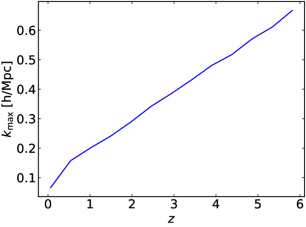
Figure 1: Maximum Fourier mode corresponding to minimum scale for perturbative analysis.

The minimum value of the wavenumber is $k_{\rm min}=k_{\rm f}$, i. ​e. the largest scale available to the survey, while the maximum value $k_{\rm max}$ corresponds to the smallest scale where the theoretical model is reliable (see Figure 1). We follow [18] and set

$$k_{\rm max}(z)=0.75\,k_{\rm NL}(z)\quad\mbox{where}\quad k_{\rm NL}(z)^{-2}=\frac{1}{6\pi^{2}}\int_{0}^{\infty}{\rm d}k\,P^{\rm L}_{\rm m}(k,z).$$ (4.3)

Here $k_{\rm NL}$ is given by the one-dimensional velocity dispersion. The choice of $k_{\rm max}$ confines the analysis within the perturbative regime, where the tree-level description offers a good agreement with numerical results [61, 62, 63, 64, 65].

The full set of parameters, which encapsulate the main contributions of uncertainty in our model, consists of 5 cosmological parameters and 11 further parameters in each redshift bin $i$:

$$\bm{\theta}(z_{i})= \Big{\{}\Omega_{\rm b},\Omega_{\rm c},h,A_{\rm s},n_{\rm s};D_{A}(z_{i}),H(z_{i}),f(z_{i}),$$

$$b_{1}(z_{i}),b_{2}(z_{i}),b_{s^{2}}(z_{i}),\sigma_{P}(z_{i}),\sigma_{B}(z_{i}),P_{\varepsilon}(z_{i}),P_{\varepsilon\varepsilon_{\delta}}(z_{i}),B_{\varepsilon}(z_{i})\Big{\}}.$$ (4.4)

We assume redshift bins are independent, so that e.g. $\partial P(\bm{k},z_{i})/\partial\theta_{\alpha}(z_{j})=0$. Then the total Fisher matrix is

$$F_{\alpha\beta}^{\rm tot}=\sum_{i=1}^{N_{z}}F_{\alpha\beta}(z_{i}).$$ (4.5)

Here $N_{z}$ is the number of redshift bins: HIRAX – $N_{z}=17$; MeerKAT L, UHF bands – $N_{z}=5,\leavevmode\nobreak\ 8$; SKAO 1, 2 bands – $N_{z}=26,\leavevmode\nobreak\ 5$. The choices for $N_{z}$ listed here, result in redshift bins of width $\Delta z\simeq 0.1$ for all surveys. For the redshift-independent cosmological parameters, the summation over all redshift bins is performed as in Equation 4.5, leading to a $5\times 5$ block in the final $F_{\alpha\beta}^{\rm tot}$, which corresponds to the summed contribution from the total redshift range. Hence, this process will take the $5+11$ square Fisher matrix from each redshift and combine them all to form the total Fisher matrix, which includes all redshift bins and has dimension $5+11N_{z}$. Further details can be found in [3].

The stochastic bias contributions $P_{\varepsilon},P_{\varepsilon\varepsilon_{\delta}}$ and $B_{\varepsilon}$, as well as the FoG parameters $\sigma_{P}$ and $\sigma_{B}$, are considered nuisance parameters and are marginalised over. Once the final total Fisher matrix is constructed, its inverse yields the minimum error on a parameter as $\sigma(\theta_{\alpha})=\sqrt{(F^{-1})_{\alpha\alpha}}$, in the case of the power spectrum and bispectrum. The forecasts from the summed power spectrum and bispectrum signal are also considered, by adding together the corresponding total Fisher matrices, i. ​e. $F_{\alpha\beta}^{P+B}=F_{\alpha\beta}^{P}+F_{\alpha\beta}^{B}$. The cross-Fisher between the power spectrum and bispectrum is neglected, since its impact on the final constraints, for the parameters of interest, is minimal [55].

4.2 Cosmological models

$\Lambda$CDM					Extensions
$\Omega_{\rm b}h^{2}$	$\Omega_{\rm c}h^{2}$	$h$	$n_{\rm s}$	$10^{9}A_{\rm s}$	$w_{0}$	$w_{a}$	$\gamma$
$0.02237$	$0.12$	$0.6736$	$0.9649$	$2.1$	$-1$	$0$	$0.55$

Table 3: Fiducial $\Lambda$CDM cosmological parameters, as measured by Planck [1], and fiducial parameters for the extensions considered here.

After marginalising over the nuisance parameters, the constraints on the remaining redshift-independent and redshift-dependent parameters, containing the key cosmological information, are transformed into constraints on parameters of the cosmological model. The baseline model is the spatially flat $\Lambda$CDM model, defined by 5 parameters:

$$\text{$\Lambda$CDM}:\big{\{}{\Omega_{\text{b}}},{\Omega_{\text{c}}},h,n_{\text{s}},A_{\rm s}\big{\}}.$$ (4.6)

To investigate further the constraining power of future HI IM surveys on deviations from the $\Lambda$CDM model, we consider two minimal extensions:

• modification of the equation of state of the dark energy:

  $$w_{\rm de}(z)=w_{0}+w_{a}\,{z\over 1+z}\,;$$ (4.7)

• modification in the growth rate of large-scale structure, via the growth index $\gamma$ [107, 108]:

  $$f(z)=\big{[}\Omega_{\rm m}(z)\big{]}^{\gamma}\,,$$ (4.8)

  where a significant deviation from $\gamma=0.55$ indicates either modified gravity or non-standard (e.g. clustering) dark energy.

The extension models are defined by

$$w_{0}w_{a}{\rm CDM}\, :\big{\{}{\Omega_{\text{b}}},{\Omega_{\text{c}}},h,n_{\text{s}},A_{\rm s},w_{0},w_{a}\big{\}},$$ (4.9)

$$\gamma{\rm CDM}\, :\big{\{}{\Omega_{\text{b}}},{\Omega_{\text{c}}},h,n_{\text{s}},A_{\rm s},\gamma\big{\}}.$$ (4.10)

Fiducial parameter values for all models are shown in Table 3.

The projection from the Fisher matrix of the initial parameter set $\theta_{\alpha}$ in Section 4.1 (after marginalising the nuisance) into the parameters $\tilde{\theta}_{A}$ of the models in Equations 4.6, 4.9, LABEL: and 4.10, is performed via the Jacobian transformation,

$$\widetilde{F}_{AB}=\big{(}J^{\rm T}\,F^{\rm tot}\,J\big{)}_{AB}=\sum_{\alpha,\beta}J_{A\alpha}\,F_{\alpha\beta}^{\rm tot}\,J_{\beta B}\qquad\mbox{where}\quad J_{A\alpha}={\partial\theta_{\alpha}\over\partial\tilde{\theta}_{A}}\,.$$ (4.11)

The precision of a particular survey on two specific parameters can be quantified through a figure of merit (FoM) [109], which is inversely proportional to the area of the $2\sigma$ contour of the two parameters, after marginalising over the rest. The ‘dark energy’ FoM is usually taken as the FoM for $w_{0}$ and $w_{a}$:

$${\rm FoM}_{w_{0}w_{a}}=\left[{\rm det}\left(\widetilde{F}_{w_{0}w_{a}}\right)\right]^{1/2}.$$ (4.12)

4.3 Statistical error

In a Gaussian approximation to the covariances of the power spectrum and bispectrum, the off-diagonal terms and the cross-covariance of $P$ and $B$ are neglected. Then the variances for the two correlators are [110, 111]:

$$\Delta P^{2}(\bm{k},z) =\frac{4\pi^{2}}{V_{\text{survey}}(z)k^{2}\Delta k(z)}P_{\rm HI}(\bm{k},z)^{2}\,,$$ (4.13)

$$\Delta B^{2}(\bm{k}_{1},\bm{k}_{2},\bm{k}_{3},z) =s_{123}\,\pi\,k_{\rm f}(z)^{3}\,\frac{P_{\rm HI}(\bm{k}_{1},z)\,P_{\rm HI}(\bm{k}_{2},z)\,P_{\rm HI}(\bm{k}_{3},z)}{k_{1}k_{2}k_{3}\,[\Delta k(z)]^{3}}\,.$$ (4.14)

Here $P_{\rm HI}$ includes the thermal noise and $s_{123}=6,2,1$, for equilateral, isosceles and non-isosceles triangles respectively. In addition, for degenerate configurations, i. ​e. $k_{i}=k_{j}+k_{m}$, the bispectrum variance should be multiplied by a factor of 2 [64, 27].

The Gaussian approximation is assumed to be accurate enough up to linear and mildly nonlinear scales and for high-density samples considered here, for both power spectrum and bispectrum, following [112, 113, 114, 115, 64]. Off-diagonal terms of the covariances are related to higher-order loop corrections [110], making the numerical implementation extremely tedious. They become important at small scales, where the Gaussian approximation breaks down. In the case of the bispectrum, these corrections affect even the variance and can have a significant effect on cosmological parameters [64].

It has also been shown that non-Gaussian contributions in the form of off-diagonal terms in the bispectrum covariance and a non-zero cross-covariance, become important even on large scales for squeezed configurations, and neglecting these contributions can lead to serious under-estimation of errors on local primordial non-Gaussianity [116, 117, 118]. We do not consider primordial non-Gaussianity here and we expect that the effect on our error estimates is smaller. Nevertheless, further work is needed in order to include non-Gaussian effects for robust error estimates on all cosmological parameters.

As a first step in this direction, we include non-Gaussian corrections to the diagonal part of the bispectrum covariance, following the prescription of [64]:

$$\Delta B_{\text{NL}}^{2}(\bm{k}_{1},\bm{k}_{2},\bm{k}_{3})= {}\Delta B^{2}(\bm{k}_{1},\bm{k}_{2},\bm{k}_{3})$$

$$+\frac{s_{123}\,\pi\,k_{\rm f}^{3}}{k_{1}k_{2}k_{3}\,(\Delta k)^{3}}\Big{[}P_{\rm HI}(\bm{k}_{1})\,P_{\rm HI}\,(\bm{k}_{2})\,P_{\rm HI}^{\text{NL}}(\bm{k}_{3})+2\;\text{perm}\Big{]},$$ (4.15)

where we omit the $z$-dependence for brevity. The nonlinear power spectrum $P_{\rm HI}^{\text{NL}}(\bm{k})$ is given by Equation 2.8 after the replacement: $P_{\rm m}(k)\rightarrow P^{\rm NL}_{\rm m}(k)-P_{\rm m}^{\rm L}(k)$, where $P^{\rm NL}_{\rm m}$ is the nonlinear matter power spectrum, described in Section 2.3.

4.4 Theoretical error

At small scales the statistical error becomes minimal, allowing for an increased signal and tighter constraints on cosmological and distance parameters, especially in the case of the bispectrum [119, 120]. However, on these scales the perturbative approach fails to describe the clustering of tracers. Even within the perturbative regime, as we approach non-linear scales, higher-order loop corrections become important. Introducing a sharp $k_{\rm max}$ cut-off excludes all scales beyond the validity of the chosen model. Nonetheless, the importance of loop corrections is gradual, indicating that neglecting them introduces biases at any $k_{\rm max}$. In the Fisher matrix analysis performed here, the uncertainty from excluding next-to-leading order corrections will be taken into account via the theoretical error approach introduced in [121].

In this formalism, theoretical errors are defined as the difference between the chosen perturbative order (e. ​g. , tree-level) and the next higher-order (e. ​g. , 1-loop). The theoretical error acts as correlated noise, forming the following covariance for the power spectrum:

$$C^{E}_{P}=E_{P}(\bm{k},z)E_{P}(\bm{k}^{\prime},z)\exp\left[-\frac{(k-k^{\prime})^{2}}{2\,\Delta k^{2}}\right],$$ (4.16)

while for the bispectrum

$$C^{E}_{B}=E_{B}(\bm{k}_{1},\bm{k}_{2},\bm{k}_{3},z)E_{B}(\bm{k}_{1}^{\prime},\bm{k}_{2}^{\prime},\bm{k}_{3}^{\prime},z)\exp\left[-\sum_{i=1}^{3}\frac{(k_{i}-k_{i}^{\prime})^{2}}{2\,\Delta k^{2}}\right].$$ (4.17)

These theoretical error covariances are added to the statistical variances, presented in the previous section, to form the final covariances that are used in the Fisher matrix formalism. The correlation length $\Delta k$ cannot be very small because the theoretical error covariance would be uncorrelated between the different momentum configurations. Here we use the value $\Delta k=0.05\;\text{$h$/Mpc}$, proposed by [122], which is motivated by the scales of the BAO wiggles. Note that the final theoretical error covariance is independent of the value of the correlation length, as long as the size of the $k$-bin is much smaller than $\Delta k$. This is true for the surveys we consider here, since the chosen binning size in the momentum space is the fundamental frequency, and $k_{f}\ll\Delta k$.

The envelopes $E_{P}$ and $E_{B}$ are given from the fitting to the desired high-order correction. For the power spectrum we use the envelope, fitted to the explicit 2-loop calculations [121]:

$$E_{P}(\bm{k},z)=D(z)^{4}P_{\rm HI}(\bm{k},z)\left(\frac{k}{0.45\;\text{$h$/Mpc}}\right)^{3.3},$$ (4.18)

where $P_{\rm HI}$ is given by Equation 2.8, but without the thermal noise contribution. For the bispectrum, we use again an envelope fitted against the 2-loop calculations [121]:

$$E_{B}(\bm{k}_{1},\bm{k}_{2},\bm{k}_{3},z)=3D(z)^{4}B_{\rm HI}(\bm{k}_{1},\bm{k}_{2},\bm{k}_{3},z)\left(\frac{k_{T}}{0.45\;\text{$h$/Mpc}}\right)^{3.3},$$ (4.19)

where $B_{\rm HI}(\bm{k}1,\bm{k}_{2},\bm{k}_{3},z)$ is given by Equation 2.9 and $k_{T}=(k_{1}+k_{2}+k_{3})/3$.

Note that the theoretical error approach, briefly described here, does not take into account FoG effect, which is not captured by perturbation theory and can become important at the loop correction level (see [123] for a discussion). Nonetheless, due to the scales considered here, the exclusion of FoG effects from the theoretical error approach is not expected to affect significantly the error covariances.

The analysis here is mostly confined to scales where the tree-level description gives accurate predictions. Hence, we do not expect the theoretical uncertainties to significantly affect our forecasts. Nonetheless, the inclusion of theoretical errors is done in order to have, as much as possible, a complete characterisation of the covariance included in the Fisher formalism.

4.5 Priors

The forecast results produced in this work, come from the Fisher information matrices. This is equivalent to assuming that all the information on the parameters comes from the likelihood, while very diffused priors are adopted. Therefore, the Fisher matrix results will be combined with the information on cosmological parameters coming from the observation of CMB performed by Planck [1]. In order to do this, we use the Markov chain that samples the posterior, from the Planck webpage, which corresponds to each fiducial cosmological model considered (Section 4.2). From the chains we compute the covariance matrix that corresponds to the subset of parameters considered here and proceed to invert the matrix in order to get the Planck Fisher matrix. The latter is then summed to the Fisher matrices of the power power spectrum and bispectrum, as well as their joined case. Effectively, we treat the Planck likelihood as a multivariate Gaussian, which is sufficient for the free cosmological parameters considered here.

5 Results

In the previous sections we outline the model, the surveys and methodology used to produce our forecasts. In this section we summarize the results on estimating the constraints on cosmological parameters coming from next-generation HI intensity experiments, in the case of the $\Lambda$CDM, $\gamma{\rm CDM}\,$and $w_{0}w_{a}{\rm CDM}\,$models, as well as on redshift dependent quantities, like cosmic distances and bias parameters. For all parameters, the forecasts are derived from the HI power spectrum, bispectrum and their joint signal (see Section 4 for details), while Planck priors are considered throughout, unless otherwise stated.

5.1 Cosmological parameters

Here we present our results on the standard $\Lambda$CDM cosmological model, by combining the Planck measurements with the forecasts coming from HI intensity mapping surveys in single-dish mode (MeerKAT and SKAO) and in interferometer mode (HIRAX-256 and HIRAX-1024). In the case of the SD mode experiments which operate in two frequency bands, the combined signal from both bands is considered (see Table 2). We exclude the redshift bins within the range $0.4\leq z\leq 0.58$ (MeerKAT UHF band) and $0.35\leq z\leq 0.49$ (SKAO band 1), in order to avoid double-counting the information within the overlapping redshifts. The marginalised relative errors on each $\Lambda$CDM cosmological parameter are presented in Table 4 (SD mode) and Table 5 (IF mode), while the 2D contours of the forecasts are shown in Figure 2.

The MeerKAT survey, once combined with Planck , provides percent-level constraints on all cosmological parameters, where the HI power spectrum and bispectrum give very similar relative errors (see Table 4). Due to the CMB external information, the summed signal from the two- and three-point correlators offers only a small improvement. As indicated by the panels in Figure 2, MeerKAT provides a marginal advantage over the Planck constraints (grey shaded contour) for most of the cosmological parameters, where the power spectrum constraints are only slightly better than those by the bispectrum.

SKAO produces moderately improved results compared to MeerKAT for all parameters, due to the larger volume and redshift range probed by SKAO, which increases the Fourier space resolution, thus improving the overall signal of the summary statistics considered. This is more evident for $\Omega_{\rm c}$ and $A_{\rm s}$. In the case of the latter, SKAO reduces the Planck errors two-fold (see bottom panels of Figure 2). Similarly to MeerKAT, the HI power spectrum and bispectrum of SKAO yield approximately equal relative errors, and the summed signal of the two correlators produces a more notable improvement compared to MeerKAT.

MeerKAT SKAO $[\%]$ P B P+B P B P+B $\Lambda$CDM $\sigma(\Omega_{\rm b})/\Omega_{\rm b}$ 0.92 (0.87) 0.92 (0.84) 0.81 (0.75) 0.66 (0.61) 0.64 (0.58) 0.56 (0.52) $\sigma(\Omega_{\rm c})/\Omega_{\rm c}$ 1.81 (1.68) 1.8 (1.62) 1.54 (1.37) 1.13 (1.0) 1.1 (0.92) 0.86 (0.74) $\sigma(h)/h$ 0.56 (0.52) 0.56 (0.5) 0.47 (0.42) 0.35 (0.31) 0.34 (0.29) 0.27 (0.23) $\sigma(n_{\rm s})/n_{\rm s}$ 0.39 (0.38) 0.39 (0.38) 0.37 (0.37) 0.35 (0.34) 0.35 (0.34) 0.33 (0.32) $\sigma(10^{9}A_{\rm s})/10^{9}A_{\rm s}$ 0.93 (0.92) 1.01 (0.95) 0.82 (0.78) 0.48 (0.47) 0.6 (0.54) 0.42 (0.39) $\gamma{\rm CDM}\,$ $\sigma(\Omega_{\rm b})/\Omega_{\rm b}$ 0.95 (0.88) 0.95 (0.85) 0.83 (0.75) 0.66 (0.61) 0.65 (0.58) 0.56 (0.52) $\sigma(\Omega_{\rm c})/\Omega_{\rm c}$ 1.88 (1.7) 1.9 (1.65) 1.59 (1.37) 1.14 (1.0) 1.12 (0.92) 0.87 (0.74) $\sigma(h)/h$ 0.58 (0.53) 0.59 (0.51) 0.49 (0.43) 0.35 (0.31) 0.35 (0.29) 0.27 (0.23) $\sigma(n_{\rm s})/n_{\rm s}$ 0.39 (0.38) 0.39 (0.38) 0.37 (0.37) 0.35 (0.34) 0.35 (0.34) 0.33 (0.32) $\sigma(10^{9}A_{\rm s})/10^{9}A_{\rm s}$ 1.22 (1.17) 1.26 (1.17) 1.13 (1.06) 0.65 (0.63) 0.88 (0.77) 0.58 (0.54) $\sigma(\gamma)/\gamma$ 12.67 (11.8) 14.89 (12.69) 10.73 (9.45) 6.11 (5.7) 8.11 (6.57) 5.05 (4.45) $w_{0}w_{a}{\rm CDM}\,$ $\sigma(\Omega_{\rm b})/\Omega_{\rm b}$ 5.06 (4.86) 5.01 (4.5) 3.95 (3.6) 2.48 (2.34) 2.55 (2.21) 1.86 (1.68) $\sigma(\Omega_{\rm c})/\Omega_{\rm c}$ 5.11 (4.88) 4.99 (4.44) 3.93 (3.54) 2.46 (2.27) 2.49 (2.11) 1.78 (1.55) $\sigma(h)/h$ 2.26 (2.17) 2.23 (2.0) 1.75 (1.59) 1.07 (1.01) 1.11 (0.95) 0.78 (0.69) $\sigma(n_{\rm s})/n_{\rm s}$ 0.42 (0.42) 0.42 (0.42) 0.42 (0.41) 0.4 (0.4) 0.4 (0.4) 0.39 (0.38) $\sigma(10^{9}A_{\rm s})/10^{9}A_{\rm s}$ 1.44 (1.42) 1.42 (1.38) 1.33 (1.29) 1.05 (1.04) 1.1 (1.06) 0.93 (0.9) $\sigma(w_{0})/w_{0}$ 31.63 (30.29) 35.04 (31.43) 25.41 (23.3) 13.69 (12.78) 16.42 (14.13) 10.41 (9.3) $\sigma(w_{\alpha})/w_{\alpha}$ 103.46 (99.03) 130.64 (117.1) 86.18 (79.42) 40.56 (37.75) 55.86 (48.32) 32.35 (29.06) $\rm FoM$ 10.8 (11.9) 7.8 (9.8) 17.3 (20.7) 73 (82) 44.7 (59) 120.5 (147) $\rm FoM_{\rm nPp}$ 5.5 (6.2) 5.5 (7.3) 11.9 (14.8) 52.7 (60.4) 39 (52.7) 99.5 (123)

Table 4: Forecasts of marginalised 1$\sigma$ relative errors (in %) on cosmological parameters in $\Lambda$CDM, $\gamma{\rm CDM}\,$and $w_{0}w_{a}{\rm CDM}\,$, for SD surveys MeerKAT and SKAO, using the combined signal of both bands of each survey (see Table 2), avoiding double-counting in overlapping redshift bins. Columns display constraints from power spectrum (P), bispectrum (B) and combination (P+B). Main results correspond to the $k_{\parallel,{\rm min}}=0.01\;\text{$h$/Mpc}$ foreground cut; the idealised case ($k_{\parallel,{\rm min}}=0$) is in parenthesis. All results assume Planck priors (see Section 4.5). Last row shows the FoM (see Section 4.2) for dark energy parameters $w_{0}$, $w_{a}$. FoM_nPp is the FoM without Planck priors.

HIRAX-256 HIRAX-1024 $[\%]$ P B P+B P B P+B $\Lambda$CDM $\sigma(\Omega_{\rm b})/\Omega_{\rm b}$ 0.39 (0.37) 0.64 (0.61) 0.38 (0.36) 0.32 (0.32) 0.43 (0.42) 0.31 (0.3) $\sigma(\Omega_{\rm c})/\Omega_{\rm c}$ 0.39 (0.23) 1.11 (1.03) 0.37 (0.23) 0.24 (0.22) 0.48 (0.46) 0.22 (0.2) $\sigma(h)/h$ 0.12 (0.08) 0.35 (0.32) 0.12 (0.08) 0.07 (0.07) 0.16 (0.15) 0.07 (0.07) $\sigma(n_{\rm s})/n_{\rm s}$ 0.15 (0.15) 0.34 (0.34) 0.15 (0.14) 0.08 (0.08) 0.25 (0.24) 0.08 (0.08) $\sigma(10^{9}A_{\rm s})/10^{9}A_{\rm s}$ 0.22 (0.22) 0.38 (0.36) 0.22 (0.22) 0.17 (0.17) 0.24 (0.23) 0.17 (0.17) $\gamma{\rm CDM}\,$ $\sigma(\Omega_{\rm b})/\Omega_{\rm b}$ 0.39 (0.37) 0.64 (0.61) 0.39 (0.36) 0.32 (0.32) 0.43 (0.42) 0.31 (0.31) $\sigma(\Omega_{\rm c})/\Omega_{\rm c}$ 0.4 (0.25) 1.12 (1.03) 0.38 (0.25) 0.29 (0.23) 0.49 (0.46) 0.25 (0.21) $\sigma(h)/h$ 0.13 (0.09) 0.35 (0.32) 0.12 (0.09) 0.1 (0.08) 0.16 (0.15) 0.09 (0.08) $\sigma(n_{\rm s})/n_{\rm s}$ 0.17 (0.15) 0.34 (0.34) 0.16 (0.15) 0.1 (0.09) 0.25 (0.24) 0.09 (0.09) $\sigma(10^{9}A_{\rm s})/10^{9}A_{\rm s}$ 0.24 (0.24) 0.56 (0.5) 0.24 (0.23) 0.17 (0.17) 0.28 (0.27) 0.17 (0.17) $\sigma(\gamma)/\gamma$ 2.41 (2.04) 16.3 (14.62) 2.34 (1.93) 1.21 (1.0) 7.51 (6.84) 1.13 (0.97) $w_{0}w_{a}{\rm CDM}\,$ $\sigma(\Omega_{\rm b})/\Omega_{\rm b}$ 1.04 (0.96) 3.61 (3.38) 1.01 (0.93) 0.74 (0.69) 1.81 (1.69) 0.68 (0.64) $\sigma(\Omega_{\rm c})/\Omega_{\rm c}$ 0.95 (0.79) 3.53 (3.3) 0.92 (0.77) 0.75 (0.66) 1.79 (1.66) 0.69 (0.61) $\sigma(h)/h$ 0.43 (0.38) 1.61 (1.51) 0.42 (0.37) 0.31 (0.29) 0.8 (0.75) 0.29 (0.27) $\sigma(n_{\rm s})/n_{\rm s}$ 0.25 (0.23) 0.4 (0.39) 0.24 (0.22) 0.2 (0.18) 0.33 (0.33) 0.19 (0.17) $\sigma(10^{9}A_{\rm s})/10^{9}A_{\rm s}$ 0.45 (0.45) 0.99 (0.96) 0.45 (0.44) 0.34 (0.3) 0.64 (0.61) 0.33 (0.29) $\sigma(w_{0})/w_{0}$ 4.65 (4.1) 18.36 (17.08) 4.5 (3.99) 3.13 (2.86) 8.67 (8.03) 2.88 (2.64) $\sigma(w_{\alpha})/w_{\alpha}$ 12.6 (10.86) 46.79 (43.68) 12.14 (10.53) 6.91 (6.32) 20.74 (19.32) 6.39 (5.85) $\rm FoM$ 904 (1091) 56 (62) 993 (1209) 3033 (3566) 298 (334) 3494 (4155) $\rm FoM_{\rm nPp}$ 775 (990) 33 (39) 873 (1119) 2712 (3276) 194 (226) 3134 (3848)

Table 5: As in Table 4 but for the IF surveys considered here.

SD mode is capable of probing better the large clustering scales [19], rendering a power spectrum analysis more appropriate. Nonetheless, the effect of the beam and the survey specifications allows for similar constraints from both correlators, once the Planck measurements are considered. From the marginalised 2D contours in Figure 2, we see that the bispectrum and power spectrum have almost the same correlations between parameters, due to the domination of the CMB signal. Adding the two- and three-point statistics offers a moderate improvement on all cosmological parameters, besides the spectral index, whose forecasts are seemingly unaffected by the inclusion of the bispectrum. This is evident for both SD surveys, as shown in Table 4.

The power spectrum is known to suffer from degeneracies between cosmological and bias parameters. Adding the information from the bispectrum introduces new shape dependencies that break various parameter degeneracies, improving the overall forecasts on cosmological parameters. For instance, the bispectrum helps to break the notorious $A_{\rm s}$ and $b_{1}$ degeneracy present in the power spectrum, since its amplitude scales like $A_{\rm s}^{2}b_{1}^{3}$. In addition, the degeneracy between $A_{\rm s}$ and $f$ is broken in a similar way. The importance of adding the bispectrum to the power spectrum data has been shown previously [124, 125, 126, 55, 123, 66, 8]. Despite the initial expectations of a minimal contribution to the cosmological constraints, when SD surveys are considered, the HI bispectrum of MeerKAT and SKAO is capable of breaking or limiting the various degeneracies between parameters and thereby provides the improvement seen in the joint forecasts. This is in agreement with recent findings for optical surveys [66, 8].

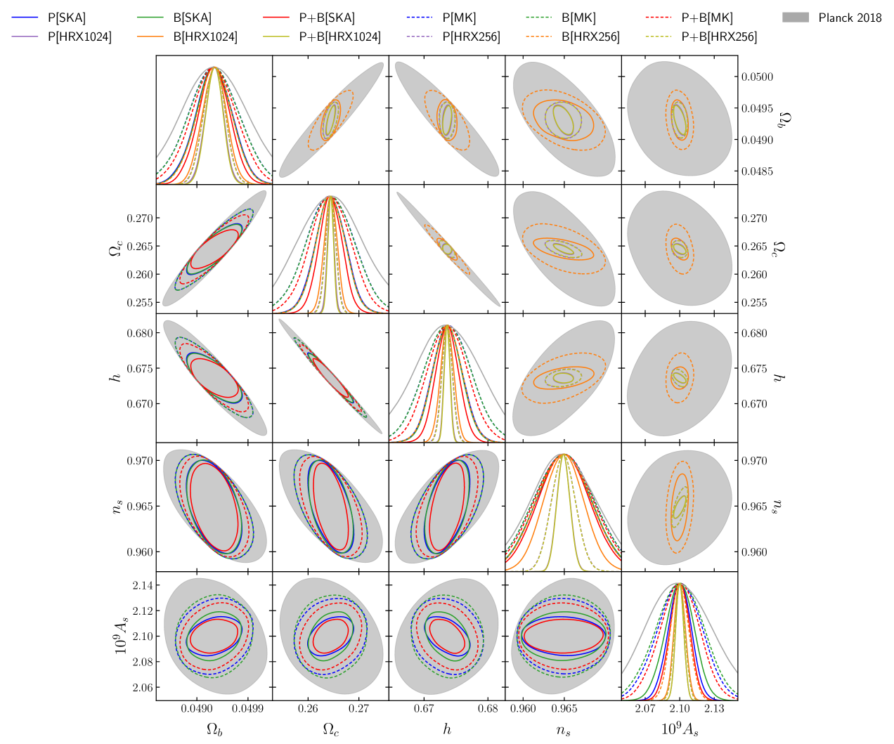
Figure 2: Marginalised 2D contours of 1$\sigma$ errors for $\Lambda$CDM parameters. Panels below the diagonal give SD surveys, panels above give IF surveys. Colour and line-type are shown at the top. All results include Planck priors; Planck results are presented for comparison. Contours correspond to the foreground cut, $k_{\parallel,{\rm min}}=0.01\;\text{$h$/Mpc}$.

The importance of adding the bispectrum can be also seen in cosmological models with a larger parameter space, since there are more degeneracies to break. This is true for the $\gamma{\rm CDM}\,$and $w_{0}w_{a}{\rm CDM}\,$models, where the addition of the bispectrum provides a significant improvement on all cosmological parameters, with the exception of $n_{\rm s}$. Naturally, this is more evident in the case of the model with the most free-parameters (i. ​e. $w_{0}w_{a}{\rm CDM}\,$), where the bispectrum not only provides an important contribution but actually dominates the joint forecasts for $\Omega_{\rm b}$, $\Omega_{\rm c}$ and $H_{0}$.

In the case of HIRAX, we consider the early-phase 256-element array and the future planned 1024-element array. For both setups, combining the HIRAX Fisher matrices with the Planck likelihoods, the errors on all $\Lambda$CDM parameters improve significantly, achieving sub-percent level, as shown by the contours of the upper triangular panels in Figure 2. The constraints are mainly driven by the HI power spectrum, as is evident from the joint forecasts in Table 5, rendering the bispectrum contribution complementary. The combined signal from the two correlators for HIRAX-1024 provides the tightest constraints presented in this work. In particular, the joint power + bispectrum without any prior information, has a precision comparable to the recent Planck results.

The improvement in the forecasts between the initial and final arrays is attributed to the higher number of elements and the amplitude of the baseline distribution $n_{\rm b}$, as given in Appendix A. This leads to a decrease in the instrumental noise [Equation 3.1] and therefore an increase in the range of available modes for the two- and three-point statistics.

In IF surveys the bispectrum has an advantage over the power spectrum, since IF mode can probe large to intermediate scales, forming a notable number of triangles and pushing the available modes to higher $k$ values, where the bispectrum signal is significantly boosted. This has been found to be true for parameters like the amplitude of primordial non-Gaussianity and bias in [18]. Despite this, for the cosmological parameters considered here, the full potential of the bispectrum is reduced in HIRAX. This is more evident in the high-noise case of HIRAX-256, where the bispectrum has negligible contribution to the final summed forecasts. HIRAX-1024, keeping all other survey specifications fixed, improves the bispectrum constraints more than it does the power spectrum, reducing the difference between the forecasts from the two correlators for all cosmological parameters.

Contrary to what was argued in the SD case, the other cosmological models do not benefit appreciably from the bispectrum information. In the $\Lambda$CDM case, bispectrum constraints could be completely neglected. The reason lies in the instrumental noise of HIRAX, which damps the signal from relevant triangle configurations, reducing the potential of the bispectrum to break degeneracies and its contribution to constraints.

The HIRAX survey characteristics offer an important advantage to the power spectrum, within the considered scale range, which provides sub-percent precision for all cosmological parameters, significantly improving over current CMB limits. Even without appreciable contribution from the bispectrum, the HIRAX forecasts are the tightest, significantly better than SKAO. In particular, the HIRAX-1024 power spectrum constraints are far stronger than those from SKAO power spectrum + bispectrum. This is despite the fact that SKAO spans a wider sky area and greater redshift range. The reason is SKAO’s low dish density (which increases the instrumental noise) and strong beam effects (which reduces the range of $k$ modes on the most important scales).

An overall conclusion is that the synergy between the LSS and CMB data is crucial in achieving robust measurements on cosmological parameters from future surveys.

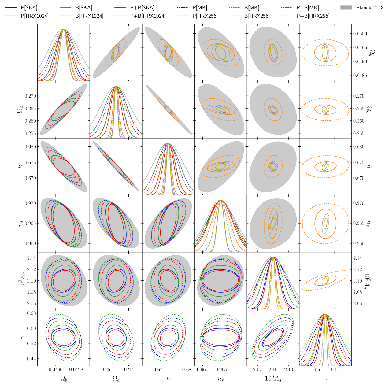
Figure 3: As in Figure 2 but for the $\gamma{\rm CDM}\,$model.

5.2 Modified gravity

Beyond the $\Lambda$CDM framework, the background and the perturbations can be modified. Modification of general relativity (GR) has been proposed as an alternative source for the accelerating expansion of the Universe observed at low redshifts [127, 128, 129, 130, 131]. There is a rich phenomenology for such models. We choose the simplest and extensively used way to probe modified growth of perturbations by testing for deviations in the growth index $\gamma$ (see Equation 4.8) from its GR value $\gamma=0.55$ (which applies to $\Lambda$CDM and also dynamical dark energy models that are non-clustering and non-interacting).

The bottom row of Figure 3 presents the marginalised 2-D contours for $\gamma$ and the other cosmological parameters for SD surveys, while the last column is for IF surveys. Relative errors on $\gamma$ are presented in Table 4 (SD surveys) and Table 5 (IF surveys). Note that the CMB data serve as priors only on the $\Lambda$CDM parameters (see Section 4.2), in order to have a clear understanding on the capabilities of each survey to robustly constrain modified gravity models.

In the case of SD experiments, the growth index can be constrained with the modest precision of $\sim 10-14\%$ by MeerKAT and $\sim 5-8\%$ by SKAO. The power spectrum yields tighter constraints than the bispectrum, in agreement with the behaviour observed for the remaining cosmological parameters, discussed in Section 5.1. Adding the bispectrum improves the power spectrum results for the two surveys by a few percent, as indicated by the joint forecasts shown in Table 4. SKAO shrinks the errors on $\gamma$ by a factor of 2 relative to MeerKAT.

In the case of HIRAX, both power and bispectrum deliver a few-percent precision on $\gamma$, with the power spectrum being the main contributor, while the bispectrum has a complementary role, with forecasts that are almost 8 times less stringent. HIRAX-1024, combined with Planck , will be capable of reaching a $1\%$ precision on $\gamma$, which would be important for eludicating the nature of gravity and any possible deviations from GR.

The marginalised contours of $\gamma$ in Figure 3 indicate that the inclusion of the growth index in the final parameter space has a minimal impact on the $\Lambda$CDM parameters. This is true for both correlators, whose contours seem to follow the same behaviour, and for all parameters, except for the amplitude of the primordial power spectrum, which exhibits sizeable degeneracies with $\gamma$. This is more evident in the case of the SD surveys, where for SKAO the errors on $A_{\rm s}$ increase by $\sim 30\%$, as shown by the relative errors of the power spectrum and bispectrum presented in Table 4. For HIRAX, the $\gamma-A_{\rm s}$ degeneracy has a small effect on the constraints of both parameters.

5.3 Dark energy

Current observations are consistent with a cosmological constant $\Lambda$, a non-dynamical dark energy model with a constant equation of state, $w_{\Lambda}=-1$. In this section, we assess the sensitivity of future and current HI experiments to departures from a cosmological constant, by using a dynamical dark energy fluid described by the redshift-dependent equation of state given in Equation 4.7 (and with sound speed of 1, which ensures that the dark energy does not cluster).

Figure 4 presents the marginalised forecasts on $w_{0}w_{a}{\rm CDM}\,$, where the contours on $w_{0},w_{a}$ are in the two bottom rows and two right-most columns, for the case of SD and IF surveys respectively. The relative errors on $w_{0}$ and $w_{a}$, together with the other cosmological parameters, are shown in Tables 4, LABEL: and 5.

In the case of SD surveys, power spectrum and bispectrum provide comparable constraints on $w_{0}$, where power-spectrum errors are a few percent smaller. Overall, MeerKAT achieves a moderate $25\%$ combined precision on $w_{0}$, while SKAO delivers $\sim 10\%$. This is not true for $w_{a}$, due to the substantial degeneracies between $w_{0}$ and $w_{a}$, as well as between the dark energy parameters and $\Omega_{\rm b}$, $\Omega_{\rm c}$ and $H_{0}$, as evident in the marginalised contours of Figure 4. MeerKAT has no constraining power on $w_{a}$, while SKAO achieves $\sim 30\%$ precision.

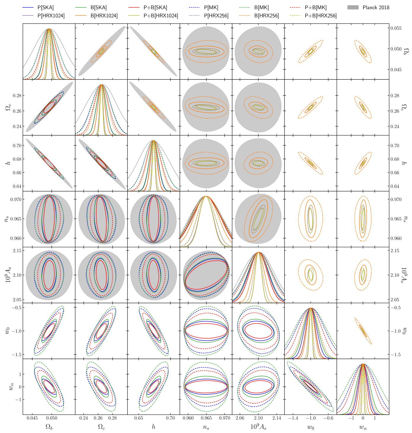
Figure 4: As in Figure 2 but for the $w_{0}w_{a}{\rm CDM}\,$model.

On the other hand, both versions of HIRAX achieve a significant improvement over the SD surveys. The constraints on $w_{0}$ and $w_{a}$ originate solely from the power spectrum, with negligible contribution from the bispectrum. Although degeneracies between $w_{0},w_{a}$ and cosmology remain (see upper triangle panels of Figure 4), HIRAX provides enough signal to produce the most stringent constraints in this work, reaching a few percent precision, when combining both correlators, on both parameters in the 1024-array setup.

In order to assess the potential of surveys in constraining dynamical dark energy, we use the FoM in Equation 4.12. We take the initial Fisher matrix with free parameters given by Section 4.1 for all redshift bins (i. ​e. $5+11N_{z}$ parameters), marginalise over the nuisance parameters and project the derived Fisher (with $5+6N_{z}$ parameters) to the parameter space of Equation 4.9, and then marginalise out all parameters except $w_{0}$ and $w_{a}$. The subsequent FoM${}_{w_{0},w_{a}}$ results are reported in the bottom rows of Tables 4, LABEL: and 5. These results include the CMB measurements, which are accounted for as priors on the $\Lambda$CDM parameters, while the FoM results, without the Planck priors, are also presented under the label ${\rm FoM_{nPp}}$.

For MeerKAT, the power spectrum and bispectrum have a similar contribution, where the addition of the bispectrum improves FoM by a factor of two. A similar improvement from the inclusion of the bispectrum is observed for SKAO, but in this case the FoM from the power spectrum surpasses that from the bispectrum by $\sim 35\%$. These findings indicate a partial breaking of degeneracies between the linear bias and primordial scalar amplitude and growth rate, when bispectrum measurements are included – which then improves the constraining power on $w_{0},w_{a}$. Adding CMB information improves the FoM further, since $A_{\rm s}$ is very well determined by Planck . The enhancement for MeerKAT is $\sim 50\%$, for SKAO it is $\sim 25\%$.

In the case of HIRAX, the power spectrum provides the largest FoM, with the bispectrum contributing $\sim 10\%$, highlighting again the inferior role of the bispectrum in HIRAX forecasts. Once CMB data are added, the FoM from the HIRAX-256 power spectrum and combined correlators improves by $\sim 15\%$, while from the bispectrum by a factor of $1.7$. For HIRAX-1024, the improvement on FoM is $\sim 12\%$ for the power spectrum and combined correlators, while for the bispectrum it is by a factor of $\sim 1.5$. These findings indicate that the bispectrum of HIRAX on its own is inadequate to break degeneracies between the considered parameters and therefore CMB data are necessary to improve the FoM, via the constraining power of Planck on $A_{\rm s}$. The improvement provided by Planck in the HIRAX FoM is more significant for the correlator with the poorest signal, i. ​e. the bispectrum. Combining the signal from both correlators for HIRAX-1024 with the CMB measurements, yields the highest FoM of this work, exceeding by far the FoM of Planck and that of recent LSS surveys (e.g. [55]). The HIRAX-1024 bispectrum alone surpasses by a significant amount the FoM from the SKAO combined correlators, in the case of the SD experiments (see Tables 4, LABEL: and 5).

5.4 Distance and growth rate measurements

Figure 5 displays the marginalised relative errors on the Hubble parameter, angular diameter distance and growth rate for all surveys considered here. Planck priors are used for the $\Lambda$CDM parameters throughout this section. The shaded regions give the upper and lower bounds corresponding to $k_{\parallel,{\rm min}}=0.01\;\text{$h$/Mpc}$ and $k_{\parallel,{\rm min}}=0$ foreground cuts, discussed in Section 3. The model assumed is the standard $\Lambda$CDM, where the mapping from $H(z)$ and $D_{A}(z)$ to the cosmological parameters, via the Jacobian transformation in Equation 4.11, is not performed. In other words, the results presented in this section utilise the Fisher matrix of the initial parameter vector [Section 4.1], which is reduced to a $5+6N_{z}$ square matrix after marginalising over the nuisance parameters.

For the SD surveys, the precision on the BAO distance scale parameters is well below $10\%$ for most of the redshift range. In particular for MeerKAT, the constraints from the two correlators are mostly on the same level; for low redshifts, the bispectrum provides smaller errors (by a few percent). The reverse is observed for higher redshifts and specifically for most of the UHF band, where constraints from the power spectrum dominate. The inclusion of the bispectrum improves significantly the power spectrum results, especially for low redshifts, keeping the precision of the joint constraints at percent level for $0.4\lesssim z\lesssim 0.6$. SKAO forecasts follow a similar pattern, providing the tightest constraints around $z\sim 0.6$, with errors larger at $z\gtrsim 1.5$. This is more evident for the angular diameter distance, where the high redshift bins of Band 1 offer no constraining power, for both correlators.

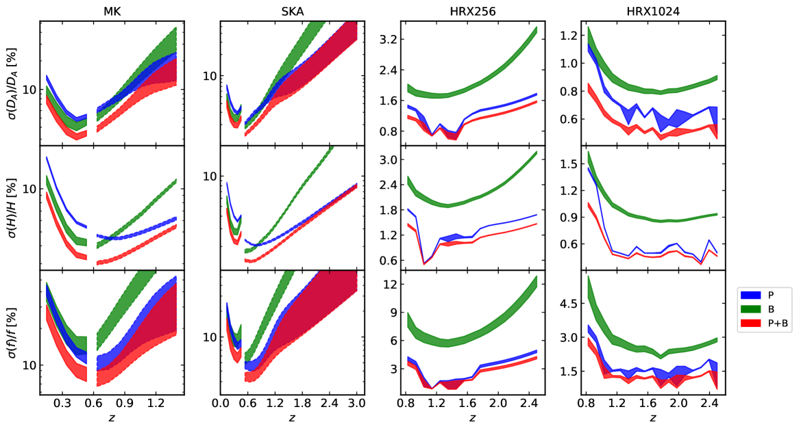
Figure 5: Forecasts of marginalised relative errors on $f$ (bottom rows), $H$ (middle) and $D_{A}$ (top), from power spectrum (blue), bispectrum (green) and combined (red). For MeerKAT and SKAO (two left columns), the low-$z$ (solid lines) and high-$z$ (dashed) bands are shown. Upper ($k_{\parallel,{\rm min}}=0.01\;\text{$h$/Mpc}$) and lower ($k_{\parallel,{\rm min}}=0$) boundaries of shaded regions correspond to the standard and idealised foreground assumptions. Gaps in SD survey curves arise since information is taken at the midpoints of the last low-$z$ and first high-$z$ bins (taking into account the removal of the lowest Band 1 bins to avoid double counting).

The SD forecasts highlight the importance of including the bispectrum when measuring the BAO distance parameters, especially for the low-$z$ bands, where instrumental noise allows access to enough scales for the bispectrum signal to break parameter degeneracies, improving on the power spectrum constraints. This behaviour is reversed for $z\gtrsim 0.8$, where the bispectrum signal does not make an important contribution. At the higher redshifts, the limitations of SD surveys (effects of beam and instrumental noise) degrade both statistics, especially the bispectrum. Angular diameter distance is afflicted the most, leading to very poor constraints for $z\gtrsim 2$. On the other hand, the relative error on the Hubble parameter are mostly $\lesssim 10\%$, reaching percent precision around $z\sim 0.6$ for both SD surveys. The effect of the standard and idealised foreground cuts is minimal for the Hubble parameter, for the whole redshift range and both surveys. This is true as well for the angular diameter distance at low redshifts, while beyond $z\sim 1$ the absence of a foreground cut has a notable effect.

Similarly to the cosmological parameters presented in the previous sections, HIRAX provides the most stringent constraints on $H$ and $D_{A}$, at sub-percent level for most of the redshift range, in the 256 and 1024 cases. Although IF surveys have the additional effect of the foreground wedge, they do not lose signal due to a wide beam at high $z$ and are able to access more of the smaller scales where signal is higher. The power spectrum consistently gives the tightest constraints, especially at high redshifts. Adding the bispectrum improves the results only marginally. For HIRAX-1024, the joint constraints saturate gradually for $z\gtrsim 1.2$. These forecasts are significantly better than for the SD surveys, in particular the high redshifts, where HIRAX achieves almost a two orders of magnitude improvement over SKAO. The HIRAX errors on the BAO distance parameters are basically unaffected by the presence of a foreground cut. This is perhaps not surprising, since IF mode surveys gain most of the signal from the intermediate and small scales.

Note that the results consider the information from CMB, which is added as priors on the $\Lambda$CDM parameters, improving the signal and breaking various degeneracies between parameters. This leads to a significant improvement of the overall forecasts on $D_{A}$ and $H$, for all surveys considered, especially for the bispectrum results, which is almost an order of magnitude. The effect on the power spectrum is more limited (by a factor of 2-3), but still noticeable. The results without the priors are not shown here for brevity.

Constraints on the growth rate $f$ in the case of MeerKAT are modest: below $10\%$ for $0.4\lesssim z\lesssim 0.8$. SKAO reaches precision of $<4\%$ for $0.6\lesssim z\lesssim 0.8$. For both SD surveys at higher redshift, the constraints worsen; for $z\gtrsim 1$ there is effectively no constraining power. At low $z$ the two correlators provide similar forecasts, and the bispectrum provides an improvement of $\sim 10\%$, mainly due to the partial breaking of the well known degeneracies between $f$, $A_{\rm s}$ and linear bias. The tree-level power spectrum is insufficient to achieve this alone and therefore the contribution from the bispectrum can help, as shown in [66, 8], at least for surveys where the three-point statistics has enough signal. At higher $z$, due to the SD beam, the contribution of the bispectrum is negligible and the forecasts are driven solely by the power spectrum.

This is also the case for HIRAX: the bispectrum contribution is minimal, but good enough to be competitive by itself, reaching a few percent precision for the entire redshift range. The power spectrum and the joint results provide a precision $\lesssim 3\%$ at all $z$ for HIRAX-256, while HIRAX-1024 doubles the precision at $z\gtrsim 1$. The presence of a foreground cut has a small effect at all $z$ for HIRAX, with a larger effect for the SD surveys, especially at high $z$.

5.5 Bias parameters

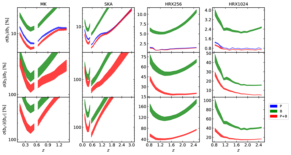
Figure 6: As in Figure 5 but for the bias parameters described in Section 2.2.

Marginalised relative errors on the linear and second-order HI bias parameters (see Section 2.2) are presented in Figure 6.

The SD surveys have modest constraining power on $b_{1}$, with maximum precision of a few percent achieved around $z\sim 0.5-0.6$. For both surveys, the constraints are driven by the power spectrum, with only a small contribution from the bispectrum. The joint errors are $<10\%$, until $z\sim 1$ for both MeerKAT and SKAO. In the case of the second-order bias parameters, MeerKAT has no constraining power, while SKAO produces errors below $100\%$ only at low redshifts, based effectively only on the bispectrum. SKAO is unusable for measuring $b_{2}$ and $b_{s^{2}}$.

The second-order bias parameters appear only in the tree-level modelling of the bispectrum, so that for the scales and models considered here, the bispectrum is the sole contributor of signal. Indeed, the main effect expected from a bispectrum analysis is the measurement of bias parameters, as shown in [55, 123, 66, 8]. However, the SD bispectrum does not contain enough information to constrain $b_{2}$ and $b_{s^{2}}$, due to unresolved degeneracies between $b_{1}$ and $b_{2}$ and between $b_{1}$ and $b_{s^{2}}$. Nonetheless, the forecasts from the joint estimation yield a significant improvement (although still non-competitive), due to the precise SD constraints on $b_{1}$ by the power spectrum, which is enough to partially break degeneracies.

For HIRAX, the forecasts again display a great improvement over the SD surveys. The bispectrum plays even less of a role in constraining linear bias than for the SD surveys. The precision on $b_{1}$ from the power spectrum and joint statistics is roughly constant over the redshift range at $\sim 1\%$ for HIRAX-256 and sub-percent for HIRAX-1024. The bispectrum, despite its negligible effect in these constraints, has enough information by itself to constrain $b_{1}$ at a few percent level, reaching $\sim 2.5\%$ at $z\gtrsim 1$ for HIRAX-1024. At high-$z$ we see that the bispectrum benefits from the larger $k_{\rm max}$ values, keeping the errors nearly constant. By contrast, the HIRAX-256 bispectrum shows rapidly growing errors at high $z$, the reason being that it is not a close-packed array like HIRAX-1024.

For $b_{2}$, the HIRAX-256 bispectrum provides poor constraints, while for $b_{s^{2}}$ there is effectively no precision from the bispectrum. Fitting simultaneously the power spectrum and bispectrum improves the results, due to the high precision on $b_{1}$ contributed by the power spectrum, which breaks degeneracies between the bias parameters. Specifically, the error on $b_{2}$ reaches $\sim 20\%$ for $z\gtrsim 1.5$, while the precision on $b_{s^{2}}$ is within $40-80\%$, which is an improvement of a factor of $\sim 2.5$. HIRAX-1024, with its close-packed array, significantly enhances precision, with a steady improvement towards high $z$, up to saturation. Bispectrum on its own reaches $\sim 15\%$ on $b_{2}$ and $\sim 40\%$ on $b_{s^{2}}$. The errors grow at lower $z$, to the point where HIRAX-1024 is unable to constrain $b_{s^{2}}$. Adding the power spectrum information again significantly improves precision: $\sim 3\%$ at high $z$ for $b_{2}$, and $\sim 20\%$, except at the lowest $z$ for $b_{s^{2}}$. Once again, HIRAX-1024 provides significant better constraints than SKAO.

The presence of a foreground cut has negligible effects on bias parameter precision for the power spectrum and joint statistics, while there is a more evident effect on the bispectrum, in particular on the $b_{2}$ constraints coming from the SD surveys and HIRAX-256.

Including the CMB measurements on the $\Lambda$CDM parameters improves the constraints on the linear bias significantly, mainly due to the breaking of degeneracies between $b_{1}$ and $A_{\rm s}$. The Planck priors affect the power spectrum forecasts the most. MeerKAT low- and high-$z$ bins show a $\sim 40\%$ improvement, with $\sim 50\%$ for the intermediate bins. For SKAO, priors mainly affect the constraints for $z<2$, with an improvement of $\sim 10-20\%$. The effect of CMB priors on the bispectrum contraints is less but still noticeable: $\sim 40-60\%$ for MeerKAT, mainly at $z\lesssim 1$; $\sim 15-20\%$ for SKAO at $z<1.5$. The remaining redshift bins are unaffected by CMB priors, mostly due to the low bispectrum signal at high-$z$ in SD surveys. The improvements from the joint power spectrum and bispectrum signal on $b_{1}$ are affected the least: $\sim 10-15\%$, with a maximum around $z\sim 0.5-0.6$, for MeerKAT; a few percent at $z<1.5$ for SKAO. The improvement is minimal for both IF arrays, and both correlators. For HIRAX-256 on $b_{1}$, it is $1-5\%$ for the power spectrum and joint signal, while the bispectrum results improve by $3-10\%$, the best at low $z$. For HIRAX-1024, there is a marginal few-percent improvement for all $z$ and both correlators.

On the other hand, $b_{2}$ and $b_{s^{2}}$ show minimal improvement for all surveys considered here and both correlators, since $b_{2}$ and $b_{s^{2}}$ are least correlated with cosmological parameters. Most of the signal is from the bispectrum, while the inclusion of priors mainly benefit the power spectrum via breaking parameter degeneracies.

6 Conclusions

In this work we examine the potential of upcoming HI intensity mapping surveys, using single-dish and interferometer modes, in constraining cosmology. These surveys enable us to probe the high-redshift Universe across wide sky area, increasing by a significant amount the observed volumes and therefore the cosmological signal of the chosen summary statistics. This could improve current measurements on cosmological and nuisance parameters. The question we try to address is: how much information is contained in the redshift space two- and three-point statistics of HI IM experiments, to constrain cosmological quantities?

The complete analytical tree-level model is used for the power spectrum and bispectrum, valid up to linear/quasi-linear clustering scales. For the power spectrum of the underlying matter field we use the non-linear treatment of the HMCode halo model [56], while for the matter bispectrum we use the tree-level prediction from standard perturbation theory. The general clustering bias prescription (Section 2.2) and redshift-space mapping (Section 2.3) are used up to the lowest non-vanishing order, i. ​e. up to leading (power spectrum) and second order (bispectrum). Additionally, the FoG effect is included via an exponential damping factor [Equations 2.12, LABEL: and 2.13], and the AP effect is incorporated in the standard way (Section 2.4). The modelling used here is a consistent approach for both statistics, since we keep the analysis well within the perturbative regime by only considering scales that satisfy $k\leq k_{\rm max}$ [Equation 4.3]. At low redshift, where non-linearity is stronger (i. ​e. smaller $k_{\rm max}$), we venture marginally into the quasi-linear regime. Due to this we also consider theoretical uncertainties in our analysis (Section 4.4). The addition of the theoretical errors to the covariance matrix takes into account the effect of neglecting higher-order effects from the chosen model, which in turn makes the parameter forecasts insensitive to the choice of the $k_{\rm max}$ value. We also take into account instrumental effects: telescope beam, instrumental thermal noise, foreground avoidance via radial and wedge cuts (see Section 3).

The analysis uses the Fisher matrix formalism to forecast constraints on cosmological parameters, modified gravity, dark energy, distance measurements and clustering bias coefficients, marginalising over FoG and stochastic bias parameters. We employ the signals from the HI power spectrum, HI bispectrum, and their combination. The results from the HI surveys are also combined with Planck constraints on the $\Lambda$CDM parameters, in the form of priors. The main results of this work are:

1. Upcoming HI IM surveys with a packed-array interferometer like HIRAX-1024, in combination with Planck measurements, could improve significantly the precision on $\Lambda$CDM parameters, reaching sub-percent levels (see Table 5).

2. For the SD surveys, the power spectrum and bispectrum in redshift space have similar constraining power on cosmological parameters, with the power spectrum being marginally better (Figure 2). Consequently, combining the information of the two correlators has a minimal impact on cosmological constraints relative to considering the power spectrum alone. For HIRAX surveys, the bispectrum contribution can be neglected (Table 5).

3. Synergy between HI surveys and CMB data is crucial for the SD surveys, in order to achieve stringent cosmological constraints. Only the summed signal from both SKAO bands can provide a meaningful improvement over Planck measurements, while MeerKAT offers negligible constraining power (Figure 2).

4. For the SD surveys the bispectrum contribution is larger, but still below the power spectrum. However, once the priors are considered, the benefit from combining the signal of the two correlators is modest (Table 4).

5. Combining HI surveys with CMB observations delivers strong potential for constraining the growth index $\gamma$. HIRAX-1024 could provide percent precision measurements from the combined signal of both correlators, while SKAO achieves $\sim 5\%$ (Table 5). The bispectrum contribution is more important for SD surveys in constraining $\gamma$, while for IF experiments it is negligible (Figure 3).

6. The dark energy equation-of-state parameters $w_{0}$ and $w_{a}$ are not well constrained by the SD mode surveys. By contrast, HIRAX-1024 could constrain them with few-percent precision (Figure 4).

7. The power spectrum and bispectrum of the SD surveys provide similar forecasts, and considering both improves the dark energy FoM by a factor $\sim 1.5-2$ relative to the power spectrum alone. The FoM of HIRAX is mainly driven by the power spectrum signal (see bottom rows of Tables 4, LABEL: and 5).

8. The combination of HIRAX and Planck reaches sub-percent precision on $D_{A}(z)$ and $H(z)$ for the combined signal (Figure 5). This could be important for elucidating the nature of the so-called ‘Hubble tension’ [132].

9. For the SD surveys, constraints on $D_{A}(z)$ and $H(z)$ are at $3-10\%$ precision for MeerKAT (except for $D_{A}$ at $z\gtrsim 1$), while SKAO achieves $1-2\%$ over the low $z$ of Band 1.

10. In the case of the growth rate $f(z)$, HIRAX can produce few-percent precision for the entire redshift range. SKAO can only do this in the low redshift slices (Figure 5).

11. An accurate assessment of the potential of future HI IM surveys to constrain cosmology, requires precision on the linear clustering bias parameter. HIRAX can achieve $<2\%$ precision on $b_{1}$ using the HI power spectrum; the bispectrum alone reaches few-percent precision, rendering its contribution negligible. A similar trend is shown for the SD surveys, where few-percent precision is achieved only at low redshifts.

12. The quadratic bias parameters, within the tree-level analysis used here, can be constrained only by the HI bispectrum. Thus, the SD surveys, due to their intrinsic limitations (see Section 3), are unable to provide useful constraints. On the other hand, HIRAX-1024, which as an IF survey achieves stronger bispectrum constraints, can deliver precision of $\sim 5\%$ on $b_{2}$ and $\sim 18\%$, on $b_{s^{2}}$ (Figure 6).

13. The standard and idealised values chosen for the radial mode cut-off in the foreground avoidance, have a minimal effect on most parameter forecasts and surveys considered here. In particular, the presence of a foreground cut seems to have a moderate effect mainly on the constraints of the growth rate and the non-linear bias, coming from the large redshift bins of the SD surveys. For these surveys and redshifts, this is also true for the angular diameter distance. We additionally checked the result of a harder foreground cut $k_{\parallel,{\rm min}}=0.05\;\text{$h$/Mpc}$, finding a negligible change in the errors, compared to the idealised case, for most of the parameters and surveys. More precisely, the only notable change is a $5-10\%$ increase in the angular diameter distance and growth rate errors from the high redshift bins of the SD surveys, while for the non-linear bias parameter the increase is within $2-5\%$.

The superior performance that is forecast for HIRAX is not unexpected. Constraining power on cosmological parameters and on the BAO distance and growth rate functions, relies on access to the higher signal on smaller scales. An interferometer such as HIRAX covers these scales particularly well, whereas SD surveys progressively lose these scales as redshift increases, due to the telescope beam [19, 18]. Indeed, HIRAX is designed as a BAO intensity mapping ‘machine’ [6]. By contrast, the SKAO interferometer was not designed with HI intensity mapping in mind, so that SKAO is better in single-dish mode for intensity mapping cosmology [5]. For cosmological constraints that require access to very large scales, such as measuring the turnover of the power spectrum [133], or probing local primordial non-Gaussianity via scale-dependent bias [134], SKAO in SD mode is more capable than an interferometer like HIRAX [18]. Finally, we should point out that pilot intensity mapping surveys (with the associated data pipeline construction) are already underway on the SKAO precursor MeerKAT [102, 135, 103, 101, 136], while the HIRAX 256-dish precursor is not yet constructed.

Appendix A Baseline distribution for HIRAX

An idealised theoretical model is proposed in [74] for the baseline density of close-packed square (HIRAX-like) and hexagonal (PUMA-like) arrays. First, the image-plane density is related to the physical density:

$$n_{\rm b}({u},z)=\lambda(z)^{2}\,n_{\rm b}^{\rm phys}(L)\quad\mbox{where}\quad L=u\,\lambda\,.$$ (A.1)

Then a fitting formula for the model of the physical baseline density is given as [74]

$$n_{\rm b}^{\rm phys}(L)=\left(\frac{N_{\rm s}}{D_{\rm dish}}\right)^{2}\,\frac{a_{1}+a_{2}\,(L/L_{\rm s})}{1+a_{3}\,(L/L_{\rm s})^{a_{4}}}\,\exp\left[-\left({L\over L_{\rm s}}\right)^{a_{5}}\right],$$ (A.2)

where $L_{\rm s}=N_{\rm s}\,D_{\rm dish}$ and $N_{\rm s}^{2}=N_{\rm dish}$. For HIRAX, $N_{\rm s}=16$ and 32 in the early and full stages respectively. The maximum baseline is the diagonal of the square array: $D_{\rm max}\approx{\sqrt{2}\,L_{\rm s}}$ [137]. The parameters in Equation A.2 for a square closely-packed array like HIRAX are [74]

$$a_{I}=\big{(}0.4847\,,\,-0.3300\,,\,1.3157\,,\,1.5974\,,\,6.8390\big{)}.$$ (A.3)

Instead of using an idealised model, we use the results from simulations of the HIRAX array [6]. These simulations are shown by the red curves in Figure 7 for 1024 (left) and 256 (right) dishes. The baseline density that follows from the fitting formula Equation A.2 is the blue curve. It is apparent that the fitting formula (blue) does not provide a very good match to the simulations (red). Different models of the baseline density $n_{\rm b}$ should each satisfy the constraint that the total number of baselines is $N_{\rm dish}(N_{\rm dish}-1)/2\approx N_{\rm dish}^{2}/2$. This implies that

$$\int{\rm d}u\,u\,n_{\rm b}\approx{N_{\rm dish}^{2}\over 4\pi}\,,$$ (A.4)

where we used ${\rm d}^{2}\bm{u}=2\pi\,u\,{\rm d}u$, assuming azimuthal symmetry. The relation Equation A.4 is satisfied by the simulated (red) and idealised (blue) curves in Figure 7.

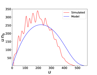
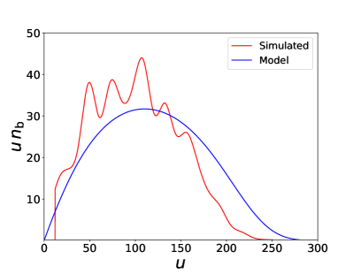
Figure 7: Comparison between the simulated baseline density (red) and the idealised model Equation A.2 (blue), for HIRAX-1024 (left) and HIRAX-256 (right).

References

- [1] Planck Collaboration, N. Aghanim, Y. Akrami, M. Ashdown, J. Aumont, C. Baccigalupi et al., Planck 2018 results. VI. Cosmological parameters, A&A 641 (2020) A6 [1807.06209].
- [2] DESI Collaboration, A. Aghamousa, J. Aguilar, S. Ahlen, S. Alam, L. E. Allen et al., The DESI Experiment Part I: Science,Targeting, and Survey Design, ArXiv e-prints (2016) [1611.00036].
- [3] Euclid collaboration, A. Blanchard et al., Euclid preparation: VII. Forecast validation for Euclid cosmological probes, Astron. Astrophys. 642 (2020) A191 [1910.09273].
- [4] LSST Dark Energy Science collaboration, R. Mandelbaum et al., The LSST Dark Energy Science Collaboration (DESC) Science Requirements Document, 1809.01669.
- [5] SKA collaboration, D. J. Bacon et al., Cosmology with Phase 1 of the Square Kilometre Array: Red Book 2018: Technical specifications and performance forecasts, Publ. Astron. Soc. Austral. 37 (2020) e007 [1811.02743].
- [6] D. Crichton et al., The Hydrogen Intensity and Real-time Analysis eXperiment: 256-Element Array Status and Overview, J. Astron. Telesc. Instrum. Syst. 8 (2022) 011019 [2109.13755].
- [7] M. G. Santos et al., Cosmology from a SKA HI intensity mapping survey, PoS AASKA14 (2015) 019 [1501.03989].
- [8] M. M. Ivanov, O. H. E. Philcox, T. Nishimichi, M. Simonović, M. Takada and M. Zaldarriaga, Precision analysis of the redshift-space galaxy bispectrum, Phys. Rev. D 105 (2022) 063512 [2110.10161].
- [9] O. H. E. Philcox and M. M. Ivanov, BOSS DR12 full-shape cosmology: CDM constraints from the large-scale galaxy power spectrum and bispectrum monopole, Phys. Rev. D 105 (2022) 043517 [2112.04515].
- [10] G. D’Amico, M. Lewandowski, L. Senatore and P. Zhang, Limits on primordial non-Gaussianities from BOSS galaxy-clustering data, 2201.11518.
- [11] G. Cabass, M. M. Ivanov, O. H. E. Philcox, M. Simonović and M. Zaldarriaga, Constraints on Multi-Field Inflation from the BOSS Galaxy Survey, 2204.01781.
- [12] A. Veropalumbo, A. Binetti, E. Branchini, M. Moresco, P. Monaco, A. Oddo et al., The galaxy 3-point correlation function: a methodological analysis, 2206.00672.
- [13] F. Rizzo, C. Moretti, K. Pardede, A. Eggemeier, A. Oddo, E. Sefusatti et al., The Halo Bispectrum Multipoles in Redshift Space, 2204.13628.
- [14] W. R. Coulton, F. Villaescusa-Navarro, D. Jamieson, M. Baldi, G. Jung, D. Karagiannis et al., Quijote-PNG: Simulations of primordial non-Gaussianity and the information content of the matter field power spectrum and bispectrum, 2206.01619.
- [15] G. Jung, D. Karagiannis, M. Liguori, M. Baldi, W. R. Coulton, D. Jamieson et al., Quijote-PNG: Quasi-maximum likelihood estimation of Primordial Non-Gaussianity in the non-linear dark matter density field, 2206.01624.
- [16] O. H. E. Philcox, M. M. Ivanov, G. Cabass, M. Simonović, M. Zaldarriaga and T. Nishimichi, Cosmology with the Redshift-Space Galaxy Bispectrum Monopole at One-Loop Order, 2206.02800.
- [17] D. Karagiannis, A. Slosar and M. Liguori, Forecasts on Primordial non-Gaussianity from 21 cm Intensity Mapping experiments, JCAP 11 (2020) 052 [1911.03964].
- [18] D. Karagiannis, J. Fonseca, R. Maartens and S. Camera, Probing primordial non-Gaussianity with the power spectrum and bispectrum of future 21 cm intensity maps, Phys. Dark Univ. 32 (2021) 100821 [2010.07034].
- [19] P. Bull, P. G. Ferreira, P. Patel and M. G. Santos, Late-time Cosmology with 21 cm Intensity Mapping Experiments, ApJ 803 (2015) 21 [1405.1452].
- [20] M. Spinelli, I. P. Carucci, S. Cunnington, S. E. Harper, M. O. Irfan, J. Fonseca et al., SKAO HI intensity mapping: blind foreground subtraction challenge, Mon. Not. Roy. Astron. Soc. 509 (2021) 2048 [2107.10814].
- [21] F. Bernardeau, S. Colombi, E. Gaztañaga and R. Scoccimarro, Large-scale structure of the Universe and cosmological perturbation theory, Phys. Rep. 367 (2002) 1 [astro-ph/0112551].
- [22] J. C. Jackson, A critique of Rees’s theory of primordial gravitational radiation, MNRAS 156 (1972) 1P [0810.3908].
- [23] A. Lewis, A. Challinor and A. Lasenby, Efficient Computation of Cosmic Microwave Background Anisotropies in Closed Friedmann-Robertson-Walker Models, ApJ 538 (2000) 473 [astro-ph/9911177].
- [24] V. Assassi, D. Baumann, D. Green and M. Zaldarriaga, Renormalized halo bias, J. Cosmology Astropart. Phys 8 (2014) 056 [1402.5916].
- [25] L. Senatore, Bias in the effective field theory of large scale structures, J. Cosmology Astropart. Phys 11 (2015) 007 [1406.7843].
- [26] M. Mirbabayi, F. Schmidt and M. Zaldarriaga, Biased tracers and time evolution, J. Cosmology Astropart. Phys 7 (2015) 030 [1412.5169].
- [27] V. Desjacques, D. Jeong and F. Schmidt, Large-scale galaxy bias, Phys. Rep. 733 (2018) 1 [1611.09787].
- [28] A. Dekel and O. Lahav, Stochastic Nonlinear Galaxy Biasing, ApJ 520 (1999) 24 [astro-ph/9806193].
- [29] A. Taruya and J. Soda, Stochastic Biasing and the Galaxy-Mass Density Relation in the Weakly Nonlinear Regime, ApJ 522 (1999) 46 [astro-ph/9809204].
- [30] T. Matsubara, Stochasticity of Bias and Nonlocality of Galaxy Formation: Linear Scales, ApJ 525 (1999) 543 [astro-ph/9906029].
- [31] U. Seljak, Analytic model for galaxy and dark matter clustering, Mon. Not. Roy. Astron. Soc. 318 (2000) 203 [astro-ph/0001493].
- [32] J. Peacock and R. Smith, Halo occupation numbers and galaxy bias, Mon. Not. Roy. Astron. Soc. 318 (2000) 1144 [astro-ph/0005010].
- [33] R. Scoccimarro, R. K. Sheth, L. Hui and B. Jain, How many galaxies fit in a halo? Constraints on galaxy formation efficiency from spatial clustering, Astrophys. J. 546 (2001) 20 [astro-ph/0006319].
- [34] F. Villaescusa-Navarro, M. Viel, K. K. Datta and T. R. Choudhury, Modeling the neutral hydrogen distribution in the post-reionization Universe: intensity mapping, JCAP 09 (2014) 050 [1405.6713].
- [35] E. Castorina and F. Villaescusa-Navarro, On the spatial distribution of neutral hydrogen in the Universe: bias and shot-noise of the HI power spectrum, MNRAS 471 (2017) 1788 [1609.05157].
- [36] J. Tinker, A. V. Kravtsov, A. Klypin, K. Abazajian, M. Warren, G. Yepes et al., Toward a Halo Mass Function for Precision Cosmology: The Limits of Universality, ApJ 688 (2008) 709 [0803.2706].
- [37] A. Cooray and R. Sheth, Halo models of large scale structure, Phys. Rep. 372 (2002) 1 [astro-ph/0206508].
- [38] F. Villaescusa-Navarro, P. Bull and M. Viel, Weighing neutrinos with cosmic neutral hydrogen, Astrophys. J. 814 (2015) 146 [1507.05102].
- [39] F. Villaescusa-Navarro et al., Neutral hydrogen in galaxy clusters: impact of AGN feedback and implications for intensity mapping, Mon. Not. Roy. Astron. Soc. 456 (2016) 3553 [1510.04277].
- [40] A. Pontzen, F. Governato, M. Pettini, C. Booth, G. Stinson, J. Wadsley et al., Damped Lyman Alpha Systems in Galaxy Formation Simulations, Mon. Not. Roy. Astron. Soc. 390 (2008) 1349 [0804.4474].
- [41] F. A. Marín, N. Y. Gnedin, H.-J. Seo and A. Vallinotto, Modeling the Large-scale Bias of Neutral Hydrogen, ApJ 718 (2010) 972 [0911.0041].
- [42] J. L. Tinker, B. E. Robertson, A. V. Kravtsov, A. Klypin, M. S. Warren, G. Yepes et al., The Large-scale Bias of Dark Matter Halos: Numerical Calibration and Model Tests, ApJ 724 (2010) 878 [1001.3162].
- [43] T. Lazeyras, C. Wagner, T. Baldauf and F. Schmidt, Precision measurement of the local bias of dark matter halos, J. Cosmology Astropart. Phys 2016 (2016) 018 [1511.01096].
- [44] T. Baldauf, U. Seljak, V. Desjacques and P. McDonald, Evidence for quadratic tidal tensor bias from the halo bispectrum, Phys. Rev. D 86 (2012) 083540 [1201.4827].
- [45] W. L. W. Sargent and E. L. Turner, A statistical method for determining the cosmological density parameter from the redshifts of a complete sample of galaxies, Astrophys. J. 212 (1977) L3.
- [46] N. Kaiser, Clustering in real space and in redshift space, MNRAS 227 (1987) 1.
- [47] A. J. S. Hamilton, Linear Redshift Distortions: a Review, in The Evolving Universe (D. Hamilton, ed.), vol. 231 of Astrophysics and Space Science Library, p. 185, 1998, astro-ph/9708102, DOI.
- [48] R. A. Battye, I. W. A. Browne, C. Dickinson, G. Heron, B. Maffei and A. Pourtsidou, H I intensity mapping: a single dish approach, MNRAS 434 (2013) 1239 [1209.0343].
- [49] P. McDonald and A. Roy, Clustering of dark matter tracers: generalizing bias for the coming era of precision LSS, J. Cosmology Astropart. Phys 8 (2009) 020 [0902.0991].
- [50] J. A. Peacock and S. J. Dodds, Reconstructing the Linear Power Spectrum of Cosmological Mass Fluctuations, MNRAS 267 (1994) 1020 [astro-ph/9311057].
- [51] W. E. Ballinger, J. A. Peacock and A. F. Heavens, Measuring the cosmological constant with redshift surveys, MNRAS 282 (1996) 877 [astro-ph/9605017].
- [52] F. Schmidt, Towards a self-consistent halo model for the nonlinear large-scale structure, Phys. Rev. D 93 (2016) 063512 [1511.02231].
- [53] R. Scoccimarro, H. M. P. Couchman and J. A. Frieman, The Bispectrum as a Signature of Gravitational Instability in Redshift Space, ApJ 517 (1999) 531 [astro-ph/9808305].
- [54] P. Gagrani and L. Samushia, Information Content of the Angular Multipoles of Redshift-Space Galaxy Bispectrum, Mon. Not. Roy. Astron. Soc. 467 (2017) 928 [1610.03488].
- [55] V. Yankelevich and C. Porciani, Cosmological information in the redshift-space bispectrum, Mon. Not. Roy. Astron. Soc. 483 (2019) 2078 [1807.07076].
- [56] A. Mead, S. Brieden, T. Tröster and C. Heymans, HMcode-2020: Improved modelling of non-linear cosmological power spectra with baryonic feedback, 2009.01858.
- [57] R. E. Smith, J. A. Peacock, A. Jenkins, S. D. M. White, C. S. Frenk, F. R. Pearce et al., Stable clustering, the halo model and non-linear cosmological power spectra, MNRAS 341 (2003) 1311 [astro-ph/0207664].
- [58] R. Takahashi, M. Sato, T. Nishimichi, A. Taruya and M. Oguri, Revising the Halofit Model for the Nonlinear Matter Power Spectrum, ApJ 761 (2012) 152 [1208.2701].
- [59] R. E. Smith and R. E. Angulo, Precision modelling of the matter power spectrum in a Planck-like Universe, Mon. Not. Roy. Astron. Soc. 486 (2019) 1448 [1807.00040].
- [60] P. Reimberg, F. Bernardeau, T. Nishimichi and M. Rizzato, Failures of Halofit model for computation of Fisher Matrices, 1811.02976.
- [61] H. Gil-Marín, J. Noreña, L. Verde, W. J. Percival, C. Wagner, M. Manera et al., The power spectrum and bispectrum of SDSS DR11 BOSS galaxies – I. Bias and gravity, Mon. Not. Roy. Astron. Soc. 451 (2015) 539 [1407.5668].
- [62] A. Lazanu, T. Giannantonio, M. Schmittfull and E. P. S. Shellard, Matter bispectrum of large-scale structure with Gaussian and non-Gaussian initial conditions: Halo models, perturbation theory, and a three-shape model, Phys. Rev. D 95 (2017) 083511 [1511.02022].
- [63] I. Hashimoto, Y. Rasera and A. Taruya, Precision cosmology with redshift-space bispectrum: a perturbation theory based model at one-loop order, Phys. Rev. D 96 (2017) 043526 [1705.02574].
- [64] K. C. Chan and L. Blot, Assessment of the information content of the power spectrum and bispectrum, Phys. Rev. D 96 (2017) 023528 [1610.06585].
- [65] A. Oddo, E. Sefusatti, C. Porciani, P. Monaco and A. G. Sánchez, Toward a robust inference method for the galaxy bispectrum: likelihood function and model selection, JCAP 03 (2020) 056 [1908.01774].
- [66] N. Agarwal, V. Desjacques, D. Jeong and F. Schmidt, Information content in the redshift-space galaxy power spectrum and bispectrum, 2007.04340.
- [67] A. Moradinezhad Dizgah, M. Biagetti, E. Sefusatti, V. Desjacques and J. Noreña, Primordial Non-Gaussianity from Biased Tracers: Likelihood Analysis of Real-Space Power Spectrum and Bispectrum, 2010.14523.
- [68] C. Alcock and B. Paczynski, An evolution free test for non-zero cosmological constant, Nature 281 (1979) 358.
- [69] H.-J. Seo and D. J. Eisenstein, Probing dark energy with baryonic acoustic oscillations from future large galaxy redshift surveys, Astrophys. J. 598 (2003) 720 [astro-ph/0307460].
- [70] Y.-S. Song, A. Taruya and A. Oka, Cosmology with anisotropic galaxy clustering from the combination of power spectrum and bispectrum, J. Cosmology Astropart. Phys 8 (2015) 007 [1502.03099].
- [71] Y. Gong, X. Chen, M. Silva, A. Cooray and M. G. Santos, The OH Line Contamination of 21 cm Intensity Fluctuation Measurements for z = 1-4, ApJ 740 (2011) L20 [1108.0947].
- [72] M. Zaldarriaga, S. R. Furlanetto and L. Hernquist, 21 Centimeter Fluctuations from Cosmic Gas at High Redshifts, ApJ 608 (2004) 622 [astro-ph/0311514].
- [73] M. Tegmark and M. Zaldarriaga, Fast Fourier transform telescope, Phys. Rev. D 79 (2009) 083530 [0805.4414].
- [74] Cosmic Visions 21 cm Collaboration, R. Ansari, E. J. Arena, K. Bandura, P. Bull, E. Castorina et al., Inflation and Early Dark Energy with a Stage II Hydrogen Intensity Mapping Experiment, arXiv e-prints (2018) arXiv:1810.09572 [1810.09572].
- [75] MeerKLASS collaboration, M. G. Santos et al., MeerKLASS: MeerKAT Large Area Synoptic Survey, in MeerKAT Science: On the Pathway to the SKA, 9, 2017, 1709.06099.
- [76] J. Fonseca, J.-A. Viljoen and R. Maartens, Constraints on the growth rate using the observed galaxy power spectrum, JCAP 12 (2019) 028 [1907.02975].
- [77] J. Shaw, K. Sigurdson, U.-L. Pen, A. Stebbins and M. Sitwell, All-Sky Interferometry with Spherical Harmonic Transit Telescopes, Astrophys. J. 781 (2014) 57 [1302.0327].
- [78] J. Shaw, K. Sigurdson, M. Sitwell, A. Stebbins and U.-L. Pen, Coaxing cosmic 21 cm fluctuations from the polarized sky using m-mode analysis, Phys. Rev. D 91 (2015) 083514 [1401.2095].
- [79] J. C. Pober, The Impact of Foregrounds on Redshift Space Distortion Measurements With the Highly-Redshifted 21 cm Line, Mon. Not. Roy. Astron. Soc. 447 (2015) 1705 [1411.2050].
- [80] R. Byrne, M. F. Morales, B. Hazelton, W. Li, N. Barry, A. P. Beardsley et al., Fundamental Limitations on the Calibration of Redundant 21 cm Cosmology Instruments and Implications for HERA and the SKA, Astrophys. J. 875 (2019) 70 [1811.01378].
- [81] T. Jacobson and R. Parentani, Horizon entropy, Found. Phys. 33 (2003) 323 [gr-qc/0302099].
- [82] S. Furlanetto, S. Oh and F. Briggs, Cosmology at Low Frequencies: The 21 cm Transition and the High-Redshift Universe, Phys. Rept. 433 (2006) 181 [astro-ph/0608032].
- [83] T.-C. Chang, U.-L. Pen, J. B. Peterson and P. McDonald, Baryon Acoustic Oscillation Intensity Mapping as a Test of Dark Energy, Phys. Rev. Lett. 100 (2008) 091303 [0709.3672].
- [84] A. Liu and M. Tegmark, A method for 21 cm power spectrum estimation in the presence of foregrounds, Phys. Rev. D 83 (2011) 103006 [1103.0281].
- [85] A. Liu and M. Tegmark, How well can we measure and understand foregrounds with 21-cm experiments?, MNRAS 419 (2012) 3491 [1106.0007].
- [86] H.-M. Zhu, U.-L. Pen, Y. Yu and X. Chen, Recovering lost 21 cm radial modes via cosmic tidal reconstruction, Phys. Rev. D 98 (2018) 043511 [1610.07062].
- [87] N. G. Karaçaylıand N. Padmanabhan, Anatomy of Cosmic Tidal Reconstruction, Mon. Not. Roy. Astron. Soc. 486 (2019) 3864 [1904.01387].
- [88] C. Modi, M. White, A. Slosar and E. Castorina, Reconstructing large-scale structure with neutral hydrogen surveys, JCAP 11 (2019) 023 [1907.02330].
- [89] J. Jasche and F. S. Kitaura, Fast Hamiltonian sampling for large-scale structure inference, MNRAS 407 (2010) 29 [0911.2496].
- [90] F. S. Kitaura, The initial conditions of the universe from constrained simulations., MNRAS 429 (2013) L84 [1203.4184].
- [91] H. Wang, H. Mo, X. Yang, Y. Jing and W. Lin, ELUCID - Exploring the Local Universe with Reconstructed Initial Density field I: Hamiltonian Markov Chain Monte Carlo Method with Particle Mesh Dynamics, Astrophys. J. 794 (2014) 94 [1407.3451].
- [92] J. Jasche, F. Leclercq and B. D. Wandelt, Past and present cosmic structure in the SDSS DR7 main sample, JCAP 01 (2015) 036 [1409.6308].
- [93] H. Wang, H. Mo, X. Yang, Y. Zhang, J. Shi, Y. Jing et al., ELUCID - Exploring the Local Universe with reConstructed Initial Density field III: Constrained Simulation in the SDSS Volume, Astrophys. J. 831 (2016) 164 [1608.01763].
- [94] U. Seljak, G. Aslanyan, Y. Feng and C. Modi, Towards optimal extraction of cosmological information from nonlinear data, JCAP 12 (2017) 009 [1706.06645].
- [95] C. Modi, Y. Feng and U. Seljak, Cosmological Reconstruction From Galaxy Light: Neural Network Based Light-Matter Connection, JCAP 10 (2018) 028 [1805.02247].
- [96] A. R. Parsons, J. C. Pober, J. E. Aguirre, C. L. Carilli, D. C. Jacobs and D. F. Moore, A Per-baseline, Delay-spectrum Technique for Accessing the 21 cm Cosmic Reionization Signature, ApJ 756 (2012) 165 [1204.4749].
- [97] J. C. Pober, A. Liu, J. S. Dillon, J. E. Aguirre, J. D. Bowman, R. F. Bradley et al., What Next-generation 21 cm Power Spectrum Measurements can Teach us About the Epoch of Reionization, ApJ 782 (2014) 66 [1310.7031].
- [98] H.-J. Seo and C. M. Hirata, The foreground wedge and 21 cm BAO surveys, Mon. Not. Roy. Astron. Soc. 456 (2016) 3142 [1508.06503].
- [99] J. C. Pober, The impact of foregrounds on redshift space distortion measurements with the highly redshifted 21-cm line, MNRAS 447 (2015) 1705 [1411.2050].
- [100] K. S. F. Fornazier et al., The BINGO Project V: Further steps in Component Separation and Bispectrum Analysis, Astron. Astrophys. 664 (2022) A18 [2107.01637].
- [101] J. Wang et al., HI intensity mapping with MeerKAT: calibration pipeline for multidish autocorrelation observations, Mon. Not. Roy. Astron. Soc. 505 (2021) 3698 [2011.13789].
- [102] Y. Li, M. G. Santos, K. Grainge, S. Harper and J. Wang, HI intensity mapping with MeerKAT: 1/f noise analysis, Mon. Not. Roy. Astron. Soc. 501 (2021) 4344 [2007.01767].
- [103] S. D. Matshawule, M. Spinelli, M. G. Santos and S. Ngobese, HI intensity mapping with MeerKAT: primary beam effects on foreground cleaning, Mon. Not. Roy. Astron. Soc. 506 (2021) 5075 [2011.10815].
- [104] A. Liu and J. R. Shaw, Data Analysis for Precision 21 cm Cosmology, Publ. Astron. Soc. Pac. 132 (2020) 062001 [1907.08211].
- [105] M. Tegmark, Measuring cosmological parameters with galaxy surveys, Phys. Rev. Lett. 79 (1997) 3806 [astro-ph/9706198].
- [106] H.-J. Seo and D. J. Eisenstein, Probing Dark Energy with Baryonic Acoustic Oscillations from Future Large Galaxy Redshift Surveys, ApJ 598 (2003) 720 [astro-ph/0307460].
- [107] O. Lahav, P. B. Lilje, J. R. Primack and M. J. Rees, Dynamical effects of the cosmological constant, Mon. Not. Roy. Astron. Soc. 251 (1991) 128.
- [108] E. V. Linder, Cosmic growth history and expansion history, Phys. Rev. D 72 (2005) 043529 [astro-ph/0507263].
- [109] A. Albrecht et al., Report of the Dark Energy Task Force, astro-ph/0609591.
- [110] E. Sefusatti, M. Crocce, S. Pueblas and R. Scoccimarro, Cosmology and the bispectrum, Phys. Rev. D 74 (2006) 023522 [astro-ph/0604505].
- [111] E. Sefusatti and E. Komatsu, Bispectrum of galaxies from high-redshift galaxy surveys: Primordial non-Gaussianity and nonlinear galaxy bias, Phys. Rev. D 76 (2007) 083004 [0705.0343].
- [112] C. Howlett and W. J. Percival, Galaxy two-point covariance matrix estimation for next generation surveys, Mon. Not. Roy. Astron. Soc. 472 (2017) 4935 [1709.03057].
- [113] A. Barreira and F. Schmidt, Response Approach to the Matter Power Spectrum Covariance, JCAP 11 (2017) 051 [1705.01092].
- [114] Y. Li, S. Singh, B. Yu, Y. Feng and U. Seljak, Disconnected Covariance of 2-point Functions in Large-Scale Structure, JCAP 01 (2019) 016 [1811.05714].
- [115] L. Blot et al., Comparing approximate methods for mock catalogues and covariance matrices II: Power spectrum multipoles, Mon. Not. Roy. Astron. Soc. 485 (2019) 2806 [1806.09497].
- [116] D. Gualdi and L. Verde, Galaxy redshift-space bispectrum: the Importance of Being Anisotropic, JCAP 06 (2020) 041 [2003.12075].
- [117] M. Biagetti, L. Castiblanco, J. Noreña and E. Sefusatti, The covariance of squeezed bispectrum configurations, JCAP 09 (2022) 009 [2111.05887].
- [118] T. Flöss, M. Biagetti and P. D. Meerburg, Primordial non-Gaussianity and non-Gaussian Covariance, 2206.10458.
- [119] C. Hahn, F. Villaescusa-Navarro, E. Castorina and R. Scoccimarro, Constraining with the bispectrum. Part I. Breaking parameter degeneracies, JCAP 03 (2020) 040 [1909.11107].
- [120] C. Hahn and F. Villaescusa-Navarro, Constraining with the bispectrum. Part II. The information content of the galaxy bispectrum monopole, JCAP 04 (2021) 029 [2012.02200].
- [121] T. Baldauf, M. Mirbabayi, M. Simonović and M. Zaldarriaga, LSS constraints with controlled theoretical uncertainties, ArXiv e-prints (2016) [1602.00674].
- [122] T. Baldauf, L. Mercolli and M. Zaldarriaga, Effective field theory of large scale structure at two loops: The apparent scale dependence of the speed of sound, Phys. Rev. D 92 (2015) 123007 [1507.02256].
- [123] A. Chudaykin and M. M. Ivanov, Measuring neutrino masses with large-scale structure: Euclid forecast with controlled theoretical error, JCAP 11 (2019) 034 [1907.06666].
- [124] H. Gil-Marín, C. Wagner, J. Noreña, L. Verde and W. Percival, Dark matter and halo bispectrum in redshift space: theory and applications, J. Cosmology Astropart. Phys 12 (2014) 029 [1407.1836].
- [125] H. Gil-Marín, W. J. Percival, L. Verde, J. R. Brownstein, C.-H. Chuang, F.-S. Kitaura et al., The clustering of galaxies in the SDSS-III Baryon Oscillation Spectroscopic Survey: RSD measurement from the power spectrum and bispectrum of the DR12 BOSS galaxies, MNRAS 465 (2017) 1757 [1606.00439].
- [126] D. Karagiannis, A. Lazanu, M. Liguori, A. Raccanelli, N. Bartolo and L. Verde, Constraining primordial non-Gaussianity with bispectrum and power spectrum from upcoming optical and radio surveys, MNRAS 478 (2018) 1341 [1801.09280].
- [127] Planck collaboration, P. A. R. Ade et al., Planck 2015 results. XIV. Dark energy and modified gravity, Astron. Astrophys. 594 (2016) A14 [1502.01590].
- [128] A. Joyce, L. Lombriser and F. Schmidt, Dark Energy Versus Modified Gravity, Ann. Rev. Nucl. Part. Sci. 66 (2016) 95 [1601.06133].
- [129] L. Amendola et al., Cosmology and fundamental physics with the Euclid satellite, Living Rev. Rel. 21 (2018) 2 [1606.00180].
- [130] A. Slosar et al., Dark Energy and Modified Gravity, 1903.12016.
- [131] N. Frusciante and L. Perenon, Effective field theory of dark energy: A review, Phys. Rept. 857 (2020) 1 [1907.03150].
- [132] E. Di Valentino, O. Mena, S. Pan, L. Visinelli, W. Yang, A. Melchiorri et al., In the realm of the Hubble tension – a review of solutions, Class. Quant. Grav. 38 (2021) 153001 [2103.01183].
- [133] S. Cunnington, Detecting the power spectrum turnover with HI intensity mapping, Mon. Not. Roy. Astron. Soc. 512 (2022) 2408 [2202.13828].
- [134] J.-A. Viljoen, J. Fonseca and R. Maartens, Multi-wavelength spectroscopic probes: prospects for primordial non-Gaussianity and relativistic effects, JCAP 11 (2021) 010 [2107.14057].
- [135] S. Paul, M. G. Santos, J. Townsend, M. J. Jarvis, N. Maddox, J. D. Collier et al., HI intensity mapping with the MIGHTEE survey: power spectrum estimates, Mon. Not. Roy. Astron. Soc. 505 (2021) 2039 [2009.13550].
- [136] S. Cunnington et al., HI intensity mapping with MeerKAT: power spectrum detection in cross-correlation with WiggleZ galaxies, 2206.01579.
- [137] S. Jolicoeur, R. Maartens, E. M. De Weerd, O. Umeh, C. Clarkson and S. Camera, Detecting the relativistic bispectrum in 21cm intensity maps, JCAP 06 (2021) 039 [2009.06197].