Milky Way’s eccentric constituents with Gaia, APOGEE & GALAH

Abstract

We report the results of an unsupervised decomposition of the local stellar halo in the chemo-dynamical space spanned by the abundance measurements from APOGEE DR17 and GALAH DR3. In our Gaussian Mixture Model, only four independent components dominate the halo in the Solar neighborhood, three previously known Aurora, Splash and Gaia-Sausage/Enceladus (GS/E) and one new, Eos. Only one of these four is of accreted origin, namely the GS/E, thus supporting the earlier claims that the GS/E is the main progenitor of the Galactic stellar halo. We show that Aurora is entirely consistent with the chemical properties of the so-called Heracles merger. In our analysis in which no predefined chemical selection cuts are applied, Aurora spans a wide range of [Al/Fe] with a metallicity correlation indicative of a fast chemical enrichment in a massive galaxy, the young Milky Way. The new halo component dubbed Eos is classified as in situ given its high mean [Al/Fe]. Eos shows strong evolution as a function of [Fe/H], where it changes from being the closest to GS/E at its lowest [Fe/H] to being indistinguishable from the Galactic low-$\alpha$ population at its highest [Fe/H]. We surmise that at least some of the outer thin disk of the Galaxy started its evolution in the gas polluted by the GS/E, and Eos is an evidence of this process.

1 Introduction

One curious thing to ponder about our Galaxy’s continuous evolution is that the guises the Milky Way takes as it transforms all remain in place – albeit somewhat hidden – for us to make sense of. Today, with new data that let us see the Galaxy in phase space (thanks to the ESA’s space observatory Gaia (Gaia Collaboration et al., 2021)) and in chemical space (thanks to massive high-resolution surveys like Apache Point Observatory Galactic Evolution Experiment (APOGEE; Abdurro’uf et al., 2022) and Galactic Archaeology with HERMES (GALAH; Buder et al., 2021a)), it is possible to reveal the Milky Way’s forgotten states and discarded guises. The Galactic halo specifically has remained the centre of intense attention thanks to its capacity to keep orbital information neatly preserved for every star deposited – this at a clear advantage compared to the studies of the disk where the past state is less straightforward to decipher due to the effects of radial mixing (see e.g., Sellwood & Binney, 2002; Schönrich & Binney, 2009; Loebman et al., 2011; Minchev et al., 2013; Frankel et al., 2020).

The halo is vast and even though its deep trawl only just started, the haul offered up by Gaia has been copious. For example, a large number of low-mass accreted systems were detected in the Solar neighbourhood (see e.g., Myeong et al., 2018a, b; Koppelman et al., 2019; O’Hare et al., 2020; Borsato et al., 2020; Limberg et al., 2021; Sofie Lövdal et al., 2022) and beyond (see e.g., Malhan et al., 2018; Ibata et al., 2019; Palau & Miralda-Escudé, 2019; Naidu et al., 2020; Yuan et al., 2020; Ibata et al., 2021). On the other hand, clear evidence for remnants of more massive galaxies consumed by the Milky Way appears rather scarce indicating a modest and restrained accretion course our Galaxy has followed.

So far, only one ancient and massive intruder has been identified unambiguously, with its body now nothing but an enormous cloud of tidal wreckage scattered throughout the inner Milky Way. The existence of a vast debris structure left behind by this merger event, known today as the Gaia Sausage/Enceladus (GS/E), was suggested before Gaia (see Evans, 2020, for the historical development). In particular, Deason et al. (2013) argued that the rapid transition in the Galactic stellar halo structural properties at break radius of 20-30 kpc is likely associated with the apocentric pile-up of a relatively early (8-10 Gyr ago) and single massive accretion event. It is hypothesised that the progenitor dwarf galaxy was massive enough for its orbit to shrink and radialise quickly as a result of a complex interplay between dynamical deceleration, host recoiling and self-friction (Vasiliev et al., 2022). Sinking deep in the heart of the Milky Way, the dwarf sprayed the bulk of its stars in a region enclosed by its last apo-centre, i.e. some $\sim 30$ kpc (see Deason et al., 2018). As a result, the region of the Galactic halo within this so-called break radius (see Deason et al., 2011) is inundated with the GS/E stars, consistently showing up as the most striking sub-structure even in relatively small volumes around the Sun (see examples of pre-Gaia hints in e.g., Chiba & Yoshii, 1998; Brook et al., 2003; Meza et al., 2005; Nissen & Schuster, 2010; Hawkins et al., 2015). Subsequently, the Gaia data made crystal clear the unusually strong radial anisotropy of the relatively metal-rich GS/E debris and helped to reveal its dominance in the Solar neighbourhood (see Belokurov et al., 2018; Myeong et al., 2018c; Haywood et al., 2018b). The genesis of the GS/E debris cloud was also unambiguously confirmed by its unique chemical fingerprint (see e.g., Helmi et al., 2018; Mackereth et al., 2019) and the large group of globular clusters (GCs) associated with it (see e.g., Myeong et al., 2018d, 2019; Massari et al., 2019). Close to the Sun, the GS/E structure has been thoroughly scrutinised both kinematically and chemically (see Necib et al., 2019; Evans et al., 2019; Sahlholdt et al., 2019; Das et al., 2020; Monty et al., 2020; Kordopatis et al., 2020; Feuillet et al., 2020; Molaro et al., 2020; Carollo & Chiba, 2021; Aguado et al., 2021a; Matsuno et al., 2021; Bonifacio et al., 2021; Feuillet et al., 2021; Buder et al., 2021b). Outside of the Solar neighborhood, fewer studies exist, nonetheless the global structure of the GS/E cloud is starting to come into focus (see e.g., Simion et al., 2019; Iorio & Belokurov, 2019; Lancaster et al., 2019; Naidu et al., 2020; Bird et al., 2021; Balbinot & Helmi, 2021; Iorio & Belokurov, 2021; Wu et al., 2022).

Two lines of enquiry help to cement the unique place the GS/E merger holds in the history of our Galaxy: its mass and the time of its arrival. Using established mass-metallicity relations (see Kirby et al., 2013), the total stellar mass of the progenitor dwarf before disruption can be gleaned from the typical metallicity of its stellar population (Belokurov et al., 2018; Feuillet et al., 2019; Naidu et al., 2021). An independent mass constraint can be obtained by scaling up the total number of globular clusters associated with the merger (Myeong et al., 2018d, 2019; Massari et al., 2019; Forbes, 2020; Callingham et al., 2022). A third method of constraining the total stellar mass is via the analysis of the GS/E chemical pattern (e.g., Fernández-Alvar et al., 2018; Helmi et al., 2018; Vincenzo et al., 2019; Mackereth et al., 2019). All of the above estimates agree that the stellar mass of the GS/E progenitor had to be of order of few $\times 10^{8}M_{\odot}$. This can be contrasted with the total stellar halo mass measurements of $\sim 10^{9}M_{\odot}$ (see Deason et al., 2019; Mackereth & Bovy, 2020). As the comparison shows, the GS/E merger must have contributed a significant fraction of the total stellar halo, perhaps as much as a half (for the inner $\sim 50$ kpc region) in agreement with local (Belokurov et al., 2018) and global (Iorio & Belokurov, 2019) estimates. In other words, a simple budget of the Galactic stellar halo leaves little room for other significant accretion events.

The dominance of the GS/E merger also makes sense when the timeline of the Galactic accretion is considered. Constraining the time of the accretion is far from straightforward. Not many asteroseismological ages exist for relatively metal-poor old stars (see Montalbán et al., 2021; Grunblatt et al., 2021; Alencastro Puls et al., 2022). These direct, albeit scarce, measurements place the epoch of the GS/E merger at 8-10 Gyr ago, in agreement with White Dwarf cooling ages (Fantin et al., 2021). The age estimates for a bulk of GS/E stars based on main-sequence-turn-off stars (Bonaca et al., 2020) and red giants (Das et al., 2020) also show good agreements with this time frame. Alternatively, the time of accretion can be obtained via the inference of the star-formation history (SFH) of the progenitor galaxy (e.g., Helmi et al., 2018; Vincenzo et al., 2019; Mackereth et al., 2019; Sanders et al., 2021). These modelling attempts agree that the dwarf’s SFH was shut down between 8 and 10 Gyr ago. Finally both the progenitor mass and the accretion time can be gauged by comparing the observed redshift $z=0$ properties of the tidal debris cloud with its numerical counterparts in galaxy formation simulations (see Belokurov et al., 2018; Fattahi et al., 2019; Bignone et al., 2019; Elias et al., 2020; Dillamore et al., 2022). Across different simulation suites, these studies find that the accretion events that lead to creation of a highly radially anisotropic metal-rich stellar halo structure near the Sun typically take place 7-10 Gyr ago and that the progenitor galaxies bring between $10^{8}$ and $10^{9}M_{\odot}$ of stars.

Does this imply that the GS/E merger is the only significant merger our Galaxy has experienced? Not necessarily. Remnants of even older interactions could potentially be hidden in the inner Galaxy, i.e. the area known as the bulge and, indeed, several such claims have been made recently (e.g., Kruijssen et al., 2019; Forbes, 2020; Horta et al., 2021). Additionally, more recent or ongoing accretion events may be lurking in the Milky Way’s outskirts. There are at least two such relatively recent and relatively massive accretion events: that of the Sagittarius dwarf galaxy (see Ibata et al., 1994; Majewski et al., 2003) and of the Magellanic System (see Wannier & Wrixon, 1972; Mathewson et al., 1974). The GS/E, the Magellanic Clouds and the Sgr dwarf are all estimated to have been hosted in dark matter halos with masses not far off $10^{11}M_{\odot}$ (see e.g., Fattahi et al., 2019; Erkal et al., 2019; Gibbons et al., 2017). In addition, tidal debris from several systems with at least an order of magnitude lower mass have also been found, e.g., Sequoia (see Myeong et al., 2018b, 2019; Matsuno et al., 2019).

The analysis reported here is inspired by the recent discoveries of a large number of diverse halo sub-structures and the need for a systematic tally of past mergers with a focus on the most important events. To our knowledge, not many attempts have been made to build a well-defined census of Galactic accretion remnants. Taking advantage of a rich but relatively small Galactic Globular Cluster dataset, several groups sought to apportion the known GCs to a small number of significant mergers (Massari et al., 2019; Kruijssen et al., 2019; Forbes, 2020; Callingham et al., 2022). However, the choices as to the decision boundaries and the number of independent components were made by hand, and therefore, unfortunately, were neither objective or reproducible (in e.g., a numerical simulation). In a similar vein, Naidu et al. (2020) suggested a break-down of the entire stellar halo accessible to the H3 survey into individual accretion events but their substructure membership, similarly to the works above, was designed by hand. Most similar to our study are the works of Das et al. (2020) and Buder et al. (2021b) who both aimed to extract the footprint of the local GS/E tidal debris in the space spanned by chemical abundances. They proceeded by modelling high-quality APOGEE and GALAH samples with a mixture of Gaussians and identifying the component representing the GS/E against the background of other Galactic populations.

The aim of our study is to build an unbiased and self-consistent inventory of the stellar halo in the vicinity of the Sun. Our main objective is to identify and characterise all of the significant independent halo components without postulating their number and their behaviour a priori. For the task in hand we will also use an approach based on a mixture of Gaussians. The stars belonging to the in situ populations such as the disk are expected to dominate the halo denizens by almost two orders of magnitude. To avoid wasting model components on known Galactic populations at the expense of the objects of our experiment, we limit the scope of our study solely to stars on orbits with high eccentricity. Thus, the stellar sample considered consists only of stars unambiguously attributed to the Galactic halo. While demanding high eccentricity ensures that the halo sample is pure, it necessarily leads to incompleteness because tidal debris with significant angular momentum will be excised. In terms of the accreted sub-structures, there are plenty of local examples with both prograde (e.g., Helmi and the associated S2 stream, Helmi et al., 1999; Myeong et al., 2018a; Aguado et al., 2021b) or retrograde (e.g., Sequoia, Myeong et al., 2018b, 2019; Matsuno et al., 2019) orbital motion.

Note that thanks to Gaia we are now certain that stars on high-eccentricity, or halo-like, orbits do not necessarily have to be accreted. As first demonstrated by Bonaca et al. (2017) roughly half of the local stellar halo is of high metallicity, i.e. [Fe/H]$>-1$ dex and is likely of in situ origin. These in situ halo stars had of course been seen before, e.g., as the high-$\alpha$ halo sequence by Nissen & Schuster (2010) and Hawkins et al. (2015) as later confirmed by e.g., Haywood et al. (2018b). The origin of the in situ halo stars with [Fe/H]$>-1$ dex has been linked to the GS/E accretion event (Gallart et al., 2019; Di Matteo et al., 2019; Belokurov et al., 2020). These stars were born in the ancient high-$\alpha$ disk of the Milky Way before the merger and subsequently “splashed” out of their circular orbits during the interaction with the GS/E progenitor, a scenario ubiquitous in numerical simulations of galaxy formation (see Belokurov et al., 2020; Grand et al., 2020; Dillamore et al., 2022). Not all of the in situ halo is splashed high-$\alpha$ disk. As Belokurov & Kravtsov (2022) demonstrate using APOGEE DR17 data, the Milky Way stars with [Fe/H]$<-1.5$ dex were likely formed in a hot and messy pre-disk state that later phase-mixed to form a centrally concentrated spheroidal in situ halo component dubbed Aurora. Conroy et al. (2022) also see evidence for an ancient Galactic pre-disk population in the low-metallicity sample of H3 stars.

This paper is structured as follows. Section 2 describes the two sets of selection cuts applied to the APOGEE and the GALAH data to produce the samples of high-quality abundance measurements analysed. As the APOGEE DR17 reports abundances with noticeably smaller uncertainties compared to GALAH we consider the APOGEE sample as our primary dataset. Section 3 briefly gives the details of the Gaussian Mixture Model methodology used here. We analyse the components extracted from APOGEE and GALAH in Section 4. Our results are placed in context and summarised in Section 5.

2 Data

We use the main and Value-Added-Catalogue (VAC) data of APOGEE Data Release (DR) 17 (Abdurro’uf et al., 2022) which provides stellar parameters, radial velocity and abundances for up to 20 chemical species for 372,458 unique targets (main red star sample). It is cross-matched with Gaia EDR3 (Gaia Collaboration et al., 2021). Using distance estimates from Bailer-Jones et al. (2021), orbital dynamics are calculated using AGAMA (Vasiliev, 2019) with the best fitting axisymmetric potential of McMillan (2017).

The sample is cleaned by rejecting any stars with STAR_BAD flag in ASPCAPFLAG, and PROGRAMNAME $=$ magclouds. Only the main red star samples with EXTRATARG $=0$ are used. To obtain a red giant star sample, logg $<3.0$ is adopted. It is further filtered with x_fe_flag $=0$, x_fe_err $<0.1$ dex for almost all elements x used in our study. The exception is [Ce/Fe], for which ce_fe_err $<0.15$ dex is used instead of $0.1$. To focus on the halo or halo-like Galactic components such as the GS/E (Belokurov et al., 2018; Haywood et al., 2018b; Myeong et al., 2018c, d) and the Splash (Belokurov et al., 2020), an eccentricity $>0.85$ cut is adopted to obtain stars on nearly radial orbits (see e.g., Belokurov et al., 2018; Myeong et al., 2018c, 2019; Mackereth et al., 2019; Buder et al., 2021b). We also require the orbital apocenter $>5$ kpc to minimize the contamination from the bulge populations (see e.g., Horta et al., 2021; Buder et al., 2021b). In addition, the distance error $<1.5$ kpc, and orbital energy $E<0$ km² s^-2 cuts are applied.

For our APOGEE-Gaia sample, we use [Fe/H], [$\alpha$/Fe], [Al/Fe], [Ce/Fe], [Mg/Mn], and the orbital energy ($E$) information, forming a 6-dimensional chemo-dynamical space to study with Gaussian Mixture Modelling (GMM). There are a total of $\approx$1700 APOGEE stars that pass our quality cuts. The choice of our 6-dimensional space is motivated by the desire to include dynamical properties ($E$) as well as the “most reliable” (or “reliable” if necessary) elemental production channels for the categories of odd-Z (Al), $\alpha$- ($\alpha$, Mg), iron-peak (Mn), and $s$-process (Ce) elements, following APOGEE’s recommendation for giant stars.

As a cross-check, we also use the main and the VAC data of GALAH DR3 (Buder et al., 2021a) which contain 678,423 spectra of 588,571 mostly nearby stars. The catalogues provide stellar parameters, radial velocity, and abundances for up to 30 chemical species. The VAC also provides various additional information including the distance estimates (see also Sharma et al., 2018) and Galactic orbital dynamics calculated using galpy (Bovy, 2015) with the McMillan (2017) potential.

We adopt the recommendations from the GALAH Collaboration for the choice of data columns and quality cuts. Our sample is first filtered with snr_c3_iraf $>30$, flag_sp $=0$. We adopt similar cuts from our APOGEE sample, with the exception of using e_x_fe $<0.2$ dex for elements x used for our study.

For our GALAH-Gaia sample, we use [Fe/H], [$\alpha$/Fe], [Na/Fe], [Al/Fe], [Mn/Fe], [Y/Fe], [Ba/Fe], [Eu/Fe], [Mg/Cu], [Mg/Mn], [Ba/Eu], as well as energy $E$. This includes similar tracers as the APOGEE sample, plus the $r$-process element (Eu) available in GALAH. Therefore for GALAH, the GMM is applied to a 12-dimensional chemo-dynamical space sampled with a total of $\approx$1100 stars that passed the above quality cuts.

3 Method

Gaussian Mixture Modelling is an unsupervised probabilistic modelling technique. It assumes that the overall distribution of some (unlabelled) data is the sum of a finite number of Gaussian distributions with unknown parameters. The optimal (maximum likelihood) model parameters can be searched for using Expectation-Maximization (EM) iterations. For our modelling, we use the Extreme Deconvolution (Bovy et al., 2011) (XD) algorithm. One attractive feature of XD is the ability to include uncertainties associated with the observed data. The maximum number of EM iterations for each XD run is $10^{9}$ by default

We run XD multiple times with different numbers of Gaussian components, from $N=1$ to $10$. For each model with $N$ Gaussians, we repeat the fit 100 times with different initial parameters randomly drawn from the parameter space. This is to insure that the algorithm obtains the true maximum likelihood, not a local maximum. The whole session of 100 random runs is also repeated multiple times to verify convergence to the best-fitting case. We check the results of the XD fitting with a different GMM package from Scikit-learn (Pedregosa et al., 2011) to demonstrate consistency.

The APOGEE sample provides abundances with noticeably smaller uncertainties as compared to GALAH. Therefore, the APOGEE-Gaia data serves as the primary sample for our study. The difference in the quality of the data is apparent in the overall level of scatter seen in each dataset.

To avoid potential over-fitting, we compute the Bayesian Information Criterion (Schwarz, 1978) (BIC) and the Akaike Information Criterion (Akaike, 1974) (AIC) for each XD run. We use the BIC score to assess the necessary number of components for each model. The lowest BIC score (highest maximum log-likelihood among all XD runs) indicates the GMM with 7 components as the optimal choice. Although the BIC scores for 5 to 8 Gaussian components cases appear relatively comparable, the 7 Gaussians case always scores the lowest BIC consistently from our repeated trials of XD fitting sessions. Since we repeat the XD fitting 100 times during each trial (with randomized initial parameters) for each model with $N$ Gaussians, we check the overall distribution of the score in each case. When compared across all models (from $N=1$ to $10$), the change in the BIC distribution shows that the median and the highest score are also the lowest at $N=7$ case in addition to the fact that it achieves the overall lowest (preferred) BIC value.

Figure 1 shows the scores from the BIC and AIC tests. For each model with $N$ Gaussians, the solid line gives the lowest score out of 100 XD runs. The dashed line is the median, and the dotted line is the highest score for each $N$ Gaussian case. Note that, although the BIC criterion provides a clear minimum, the AIC does not. The differences between AIC and BIC are discussed in standard texts on Bayesian model fitting using information criteria (e.g., Gelman et al., 2015). Here, we merely note that model selection is a difficult task, without a clear-cut answer as to which information criteria works best.

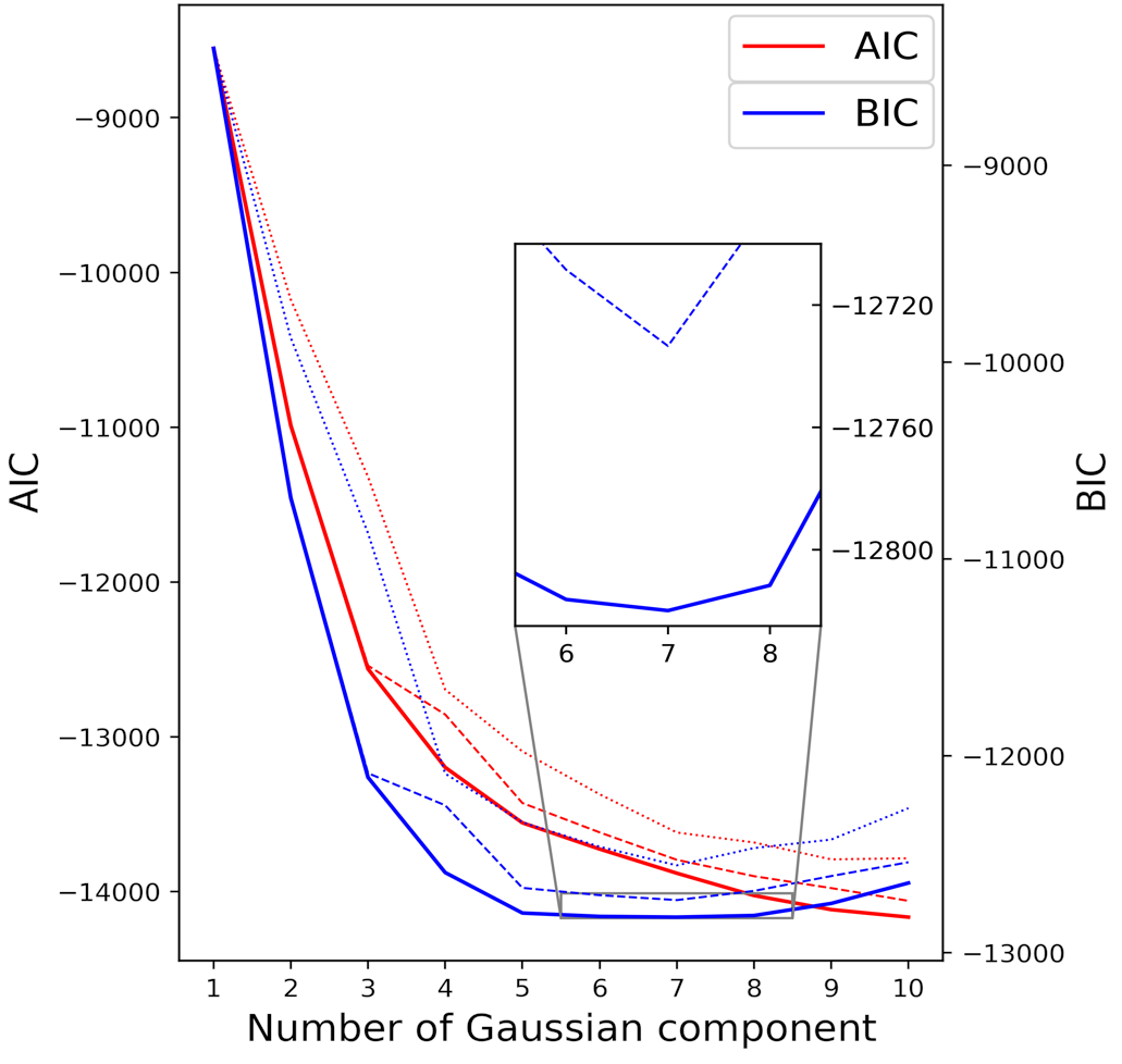
Figure 1: Red (blue) curves show AIC (BIC) performance for the APOGEE sample as a function of the number of Gaussian components. For each number of components, the GMM fit is performed a large number of times starting from random initial conditions to ensure convergence and to investigate scatter in obtained solutions. For each number of components probed, solid line gives the lowest (best) AIC/BIC score, dashed line corresponds to the median, and dotted to the highest score. The BIC test indicates the GMM with 7 Gaussian components as the optimal case. The zoom-in panel shows the BIC result around the best score.

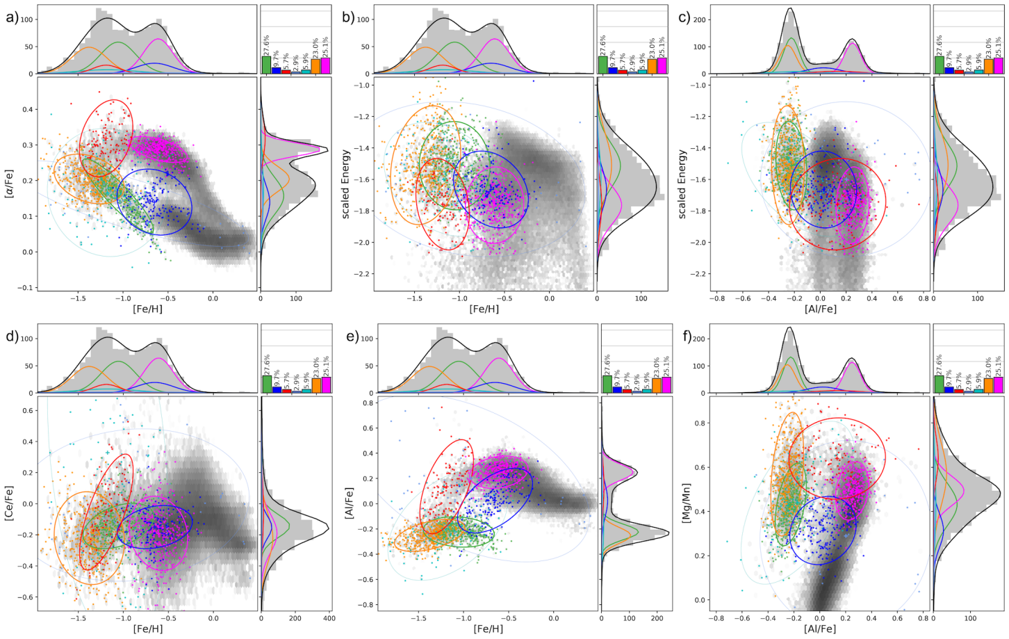
Figure 2: Distribution of Galaxy’s eccentric populations in APOGEE-Gaia sample in chemo-dynamical spaces. The GMM identified components are marked with $2\sigma$ ellipses. The Splash and Aurora are marked with magenta and red, The GS/E (GS/E₁ & GS/E₂ enclosing the metal-richer and metal-poorer portion) components are marked with green and yellow. The Eos is marked with blue. Two background components with low weight and no clear physical trend are marked with cyan and navy. The modelled distribution for each component and the total sum (black line) is marked in 1-dimensional histogram along each dimension at the top and the right side of each panel together with the background histogram marking the distribution of the stars used for the GMM. The weight of each component is marked at the top-right corner of each panel. 2-dimensional density histogram of the whole APOGEE-Gaia dataset is shown as a greyscale background as a reference. Each panel shows different 2-dimensional projection of the original 6-dimensional chemo-dynamical space used for the GMM, a): [$\alpha$/Fe] vs [Fe/H], b): scaled energy vs [Fe/H], c): scaled energy vs [Al/Fe], d): [Ce/Fe] vs [Fe/H], e): [Al/Fe] vs [Fe/H], f): [Mg/Mn] vs [Al/Fe].

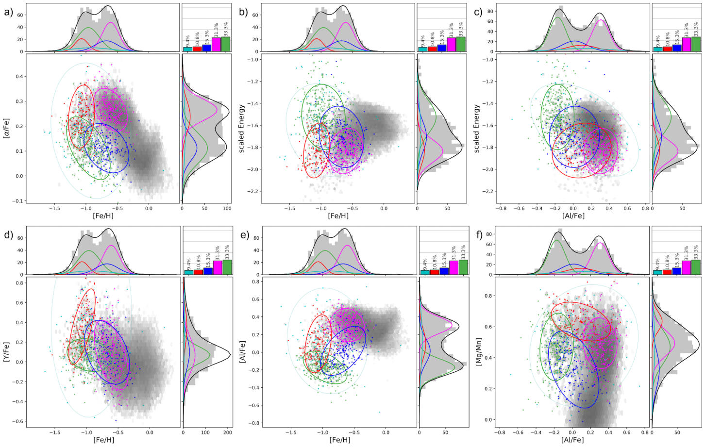
Figure 3: Distribution of Galaxy’s eccentric populations in chemo-dynamical spaces similar to Figure 2 but with GALAH-Gaia sample. For GALAH-Gaia sample 12-dimensional chemo-dynamical space is used for the GMM and the projections corresponding to Figure 2 are shown. The GS/E component is marked with green (see Section 4 for more detail). Panel d) shows [Y/Fe] vs [Fe/H].

Figure 4: Distribution of Galaxy’s eccentric populations in GALAH-Gaia sample in chemo-dynamical spaces similar to Figure 3 but for different 2-dimensional projection of the original 12-dimensional chemo-dynamical space used for the GMM, a): [Mn/Fe] vs [Fe/H], b): [Na/Fe] vs [Fe/H], c): [Mg/Cu] vs [Na/Fe], d): [Ba/Fe] vs [Fe/H], e): [Eu/Fe] vs [Fe/H], f): [Ba/Eu] vs [Fe/H].

Table 1: Summary of GMM fit result for APOGEE-Gaia sample

Component	Weight	Count	[Fe/H]	[$\alpha$/Fe]	Energy	[Ce/Fe]	[Al/Fe]	[Mg/Mn]
	(%)				($10^{5}$ km2 s-2)
GS/E1	27.6	445	$-1.05\pm 0.20$	$0.16\pm 0.05$	$-1.51\pm 0.14$	$-0.14\pm 0.07$	$-0.22\pm 0.06$	$0.43\pm 0.09$
GS/E2	23.0	396	$-1.38\pm 0.20$	$0.20\pm 0.03$	$-1.51\pm 0.19$	$-0.22\pm 0.15$	$-0.25\pm 0.06$	$0.57\pm 0.14$
Splash	25.1	417	$-0.61\pm 0.16$	$0.29\pm 0.02$	$-1.76\pm 0.12$	$-0.19\pm 0.12$	$0.25\pm 0.06$	$0.49\pm 0.07$
Aurora	5.7	112	$-1.19\pm 0.15$	$0.32\pm 0.05$	$-1.76\pm 0.15$	$-0.05\pm 0.19$	$0.13\pm 0.19$	$0.64\pm 0.09$
Eos	9.7	177	$-0.65\pm 0.21$	$0.14\pm 0.05$	$-1.66\pm 0.12$	$-0.15\pm 0.07$	$0.03\pm 0.13$	$0.31\pm 0.08$
back1	5.9	105	$-1.17\pm 0.33$	$0.17\pm 0.09$	$-1.60\pm 0.18$	$0.33\pm 0.63$	$-0.17\pm 0.22$	$0.44\pm 0.18$
back2	2.9	54	$-0.92\pm 0.66$	$0.14\pm 0.06$	$-1.60\pm 0.25$	$-0.01\pm 0.25$	$0.20\pm 0.33$	$0.29\pm 0.22$
GS/Esum	50.6	841	$-1.20\pm 0.25$	$0.18\pm 0.05$	$-1.50\pm 0.18$	$-0.18\pm 0.15$	$-0.24\pm 0.07$	$0.49\pm 0.14$
backsum	8.8	159	$-1.08\pm 0.47$	$0.16\pm 0.08$	$-1.59\pm 0.22$	$0.21\pm 0.56$	$-0.05\pm 0.31$	$0.39\pm 0.21$

Note. — Weight is the GMM estimated weight of each component. Count is the number of stars assigned to each component based on the membership probability. See Section 4.1 for more detail. GS/E_sum row marks the combined properties of GS/E₁ and GS/E₂ (metal-richer and metal-poorer portion of the GS/E). back_sum row marks the combined properties of two background components, back1 and back2.

Table 2: Summary of GMM fit result for GALAH-Gaia sample

Component	Weight	Count	[Fe/H]	[$\alpha$/Fe]	Energy	[Ba/Fe]	[Y/Fe]	[Na/Fe]	[Al/Fe]	[Mn/Fe]	[Mg/Cu]	[Mg/Mn]	[Eu/Fe]	[Ba/Eu]
	(%)				($10^{5}$ km2 s-2)
GS/E	33.3	354	$-0.96\pm 0.17$	$0.11\pm 0.06$	$-1.52\pm 0.15$	$0.38\pm 0.18$	$0.07\pm 0.08$		$-0.17\pm 0.09$	$-0.37\pm 0.09$	$0.61\pm 0.06$	$0.47\pm 0.11$	$0.47\pm 0.10$	$-0.09\pm 0.21$
Splash	31.3	337	$-0.61\pm 0.13$	$0.27\pm 0.04$	$-1.83\pm 0.10$	$0.17\pm 0.23$	$0.07\pm 0.18$		$0.31\pm 0.09$	$-0.18\pm 0.06$	$0.30\pm 0.11$	$0.49\pm 0.08$	$0.28\pm 0.07$	$-0.11\pm 0.25$
Aurora	10.8	125	$-1.07\pm 0.10$	$0.24\pm 0.06$	$-1.83\pm 0.12$	$0.48\pm 0.25$	$0.36\pm 0.19$		$0.10\pm 0.16$	$-0.38\pm 0.08$	$0.59\pm 0.08$	$0.63\pm 0.06$	$0.31\pm 0.11$	$0.17\pm 0.28$
Eos	15.3	168	$-0.67\pm 0.18$	$0.11\pm 0.05$	$-1.71\pm 0.14$	$0.34\pm 0.20$	$0.10\pm 0.16$		$0.02\pm 0.14$	$-0.22\pm 0.09$	$0.32\pm 0.19$	$0.32\pm 0.12$	$0.32\pm 0.13$	$0.02\pm 0.22$
back	9.4	106	$-0.92\pm 0.32$	$0.18\pm 0.14$	$-1.64\pm 0.21$	$0.81\pm 0.56$	$0.43\pm 0.49$		$0.13\pm 0.30$	$-0.31\pm 0.20$	$0.53\pm 0.21$	$0.48\pm 0.20$	$0.45\pm 0.23$	$0.36\pm 0.50$

Note. — Weight is the GMM estimated weight of each component. Count is the number of stars assigned to each component based on the membership probability. See Section 4.1 for more detail.

4 The Galaxy’s eccentric constituents

4.1 GMM view of the local halo

GMM is an unsupervised probabilistic modelling technique. Naturally enough, it recovers the chemical signatures of the three known eccentric components of the Galaxy, namely the GS/E, the Splash and Aurora. This is in itself valuable as it confirms earlier results derived by extracting samples of these populations by hand-made cuts. Equally, this confirmation adds extra confidence to the GMM’s results when the method breaks completely new ground.

For each GMM component in the APOGEE-Gaia sample, the parameters describing the weight (fractional contribution), the mean and the standard deviation $\sigma$ of the model are presented in Table 1. The value for the combined GS/E population is also marked as GS/E_sum. The sum of the two low-amplitude physically implausible components, associated with the background, (back₁, back₂) are also marked as back_sum for a reference. Figure 2 shows several 2-dimensional projections of the original 6-dimensional chemo-dynamical APOGEE-Gaia space used for the GMM. The best-fit model contains 7 Gaussian components shown with 2$\sigma$ ellipses. As a result of the fit, each star in the sample has a probability of belonging to an individual Gaussian component. By comparing these probabilities, the component membership of each star is established. There can be cases that a star has comparable probabilities between multiple components, making the classification less certain. Although this can result in slight deviation between the GMM estimated weight and the number of stars assigned to each component, we note that this deviation is within a small fraction. For our samples, there are $<1\%$ in APOGEE and $<2\%$ in GALAH that the difference between the highest and the second-highest component probabilities for each star is less than 0.05 (probability ranges from 0 to 1). While we use the stars with high orbital eccentricity ($e>0.85$) for our GMM study, the density histogram of the whole APOGEE-Gaia dataset is also shown as a 2-dimensional greyscale background for each projection to put the properties of the model Gaussian components into context.

We also apply the XD algorithm to GALAH-Gaia, which include additional tracers. For the odd-Z and iron-peak elements, Na and Cu are included in addition to the abundances used in the fitting of the APOGEE-Gaia sample. For the $s$-process, Y and Ba are used instead of Ce. In the case of the $r$-process, Eu is included. This is particularly desirable, as no $r$-process tracer is available in the APOGEE-Gaia sample. Similar to the APOGEE-Gaia sample, the parameters of each of the components identified by the GMM in GALAH are listed in Table 2. Figures 3 and 4 shows sets of 2-dimensional projections among the 12-dimensional GALAH sample space.

The GMM for both samples finds strong evidence for 4 independent, physically plausible components. These comprise the three known constituents, together with an entirely new population called Eos. Only one of these components is of accreted origin, namely the GS/E. This dominates the eccentric sample locally. Importantly, there is no clear chemical evidence for another major accretion event in the Solar neighborhood. This makes sense – only the most massive accreted objects can fall deep into the potential well of the Galaxy. Innumerable minor accretion events have indeed occurred (e.g., Myeong et al., 2018a, b; Koppelman et al., 2019; O’Hare et al., 2020; Borsato et al., 2020; Limberg et al., 2021; Sofie Lövdal et al., 2022), but their residues are – relatively speaking – inconsequential for the local sample.

There are other reassuring properties of the GMM results that add credibility to its decomposition. First, there is consistency between the results when applied to APOGEE-Gaia and GALAH-Gaia in terms of the number and properties of the components. Both datasets provide evidence for 4 physically-motivated components. Secondly, whenever there are elements in common between the two samples, then there is consistency in the results for the 4 components, as shown for example in Figs. 2 and  3. Thirdly, there is also consistency between APOGEE-Gaia and GALAH-Gaia for the same groups of elements. For example, in odd-Z ([Al/Fe], [Na/Fe]), $\alpha$- ([$\alpha$/Fe]) or iron-peak ([Mn/Fe]) elemental planes, the GMM clearly sees the same evolutionary trends in all 4 populations, irrespective of whether the APOGEE-Gaia and GALAH-Gaia datasets are used.

The only substantial difference is in the fractional contributions of the 4 components. For example, the GMM judges that GS/E comprises a majority of the local halo when applied to APOGEE-Gaia, but only a third in GALAH-Gaia. Here, we readily concede that the relative weightings of the populations are due to the surveys’ distinct selection functions. For example, the GALAH-Gaia sample is undernourished in stars below [Fe/H] $<-1.3$ dex, so the GMM over-weights the Splash, the Aurora and the Eos, while under-weighting the GS/E, as compared to APOGEE-Gaia.

Another interesting difference is that, in APOGEE-Gaia, the GMM is powerful enough to split the GS/E into two separate, but closely-related, Gaussians. These correspond to the $\alpha$ plateau and the knee of the progenitor dwarf. In APOGEE-Gaia, the GS/E population is so well represented, especially at low metallicities, that the GMM can even break down the population into its internal chemical structure.

Finally, in both the APOGEE-Gaia and GALAH-Gaia, the GMM finds low-weight “background populations”. These are consistent with an outlier contribution, as they do not show physically plausible chemo-dynamical trends. For example, they have very large and thus physically implausible dispersion in most elements encompassing giant swaths of the abundance space. Since there will clearly be a discrepancy between the true distribution of each genuine Galactic population and the Gaussian model assumed by the GMM, residuals between the data and the model are expected. Such residuals across the sample space can easily be absorbed into a broad, low-weight and featureless background (Gaussian) density GMM component.

We now discuss the GMM results for the 4 physically plausible components in turn. For the GS/E and the Splash, this is largely a confirmation and amplification of earlier results, though now obtained by an unsupervised learning method. For the Aurora, the GMM identifies completely new chemical trends, e.g. in Eu, Y and Ba, whilst Eos is here identified and described for the very first time.

4.2 GS/E

The GS/E takes up $\approx 51\%$ of eccentric stars in the APOGEE-Gaia sample ($\approx 33\%$ in the GALAH-Gaia sample). GS/E has an ex situ origin, having formed as a result of the disruption of a relatively massive galaxy. The mass of the progenitor dwarf has to be high to shrink and radialize the orbit (Vasiliev et al., 2022), so that the bulk of its stars are deposited into the inner regions of the Milky Way’s halo. Only the most massive objects are able to sink sufficiently deep in the host’s potential (e.g., dynamical friction being stronger for massive acquisitions) and contribute a sizeable fraction of their phase-mixed (and thus covering a significant volume) tidal debris in a given small region. Of all the components, the GS/E shows the highest mean orbital energy with the widest spread, as well as the lowest metallicity. This is also in accord with its ex situ origin and with its debris being spread during the interaction (see e.g., panels b) and c) of Figures 2 and 3.

With a progenitor mass of at least 1/10 of the Milky Way (e.g., Belokurov et al., 2018) at the time of merger, GS/E shows a metal-poor $\alpha$-knee at [Fe/H] $\approx-1.3$ (e.g., Helmi et al., 2018; Mackereth et al., 2019). Its inefficient star-formation is linked to its meagre enrichment in the odd-Z elements, which is reflected in the GS/E’s low [Al/Fe] and [Na/Fe] level.

Since our APOGEE-Gaia sample extends down to lower metallicity, we can trace the GS/E’s behavior at low metallicity better than in GALAH-Gaia. In Figure 2, we see that the GS/E population splits into two. The two components have similar mean energy. However, the low metallicity portion (GS/E₂, yellow) shows a wider spread across the orbital energy range and also reaches down to lower orbital energies compared to its higher metallicity counterpart (GS/E₁, green). Note that even in the absence of dynamical friction, the dwarf progenitor’s stars could cover a wide range of energies with leading and trailing debris occupying preferentially lower and higher energies correspondingly (see also, D’Onghia et al., 2009, for complications in the case of a massive and rotating progenitor). This effect will blur any simple metallicity-energy correlation and could also result in the lower metallicity debris showing a wider spread, including the higher and lower ends of the orbital energy range. GS/E₁ and GS/E₂ correspond to (i) the knee/decline in $\alpha$ and in [Al/Fe] with increasing contribution from SN Ia and (ii) high-$\alpha$ plateau and slowly rising [Al/Fe]. The two GS/E components also show different behaviour in Ni, another element sensitive to SN Ia explosions.

In the APOGEE-Gaia data, the GS/E population covers a wide range of metallicities. So, we can expect its chemical distribution (e.g., [Fe/H], [$\alpha$/Fe], [Al/Fe], [Mg/Mn]) to be considerably non-Gaussian. Since GMM assumes its components are Gaussian, it struggles to reproduce such an extended component with a single Gaussian. This is why the GS/E population in our APOGEE-Gaia sample splits into two separate but related Gaussians. For example, [Fe/H] $\approx-1.3$ is a pivotal point where GS/E’s slope undergoes a small but noticeable change in [$\alpha$/Fe] and [Al/Fe] as a function of [Fe/H] (e.g., panel a) of Figure 2). GS/E’s [Al/Fe] shows a mild increase along the metallicity range probed, reaching its peak around [Fe/H] $\approx-1.3$, and turns to a decreasing trend beyond this metallicity. This pattern is in good agreement with the earlier analysis of APOGEE data reported by e.g., Hasselquist et al. (2021) and Belokurov & Kravtsov (2022).

The unbiased GMM decomposition also recovers the fact that the GS/E is high in [Eu/Fe] and [Eu/Mg], consistent with previous studies (Aguado et al., 2021a; Matsuno et al., 2021). Eu and Mg are both good tracers for Core-Collapse Supernovae (CCSNe) contribution in star formation history as they are believed to be produced from massive stars most exclusively. But, in case of Eu ($r$-process element), Neutron Star Mergers (NSMs) are another considerable source of enrichment  (see e.g., Kobayashi et al., 2020). These two $r$-process channels have distinct timescales – CCSNe (NSMs) are known for prompt (delayed) $r$-process production, respectively. This means for a system with longer duration of star formation the [Eu/Mg] level will increase, as it will give more chance for the delayed Eu enrichment of NSMs to be reflected. Thus Eu trends mentioned above are a consequence of the longer star formation duration for the GS/E than the Milky Way. The Milky Way progenitor’s has a much more vigorous and efficient star formation than GS/E progenitor.

4.3 Splash

The Splash is another major component in our high-eccentricity sample. Compared to GS/E, the orbital energy of the Splash stars is also low. This is consistent with the idea that it is an in situ population kicked out of the Galactic disk by the GS/E merger.

The Splash contributes $\approx 25\%$ in APOGEE-Gaia and $\approx 31\%$ in GALAH-Gaia sample. The differences between the two datasets in the fractional contribution of this population are likely due to the differences in the surveys’ selection functions, particularly the metallicity range probed. For example, our GALAH-Gaia sample has very few stars below [Fe/H]$<-1.3$ dex. Since the GS/E population is dominant below this metallicity, GS/E’s total weight in the GALAH sample appears to be lower compared to the APOGEE sample which extends down to lower metallicity.

In comparison to GS/E, the Splash population shows a distinctively high [Fe/H], [$\alpha$/Fe] and [Al/Fe] abundances which are the known characteristics of this high-$\alpha$ in situ population (Nissen & Schuster, 2010; Hawkins et al., 2015; Haywood et al., 2018b; Di Matteo et al., 2019; Belokurov et al., 2020). The observed spread in chemical element distributions are narrow in general for the Splash, especially for [$\alpha$/Fe] and [Al/Fe], whilst the metallicity is limited to $-0.9<$[Fe/H]$<-0.3$ dex. The main advance in this paper is here the chemical properties of the Splash have been “discovered” by an unbiased GMM decomposition rather than extrapolated from hand-made cuts.

There is remarkable consistency across all chemical dimensions between the Splash and the high-$\alpha$ disc. This is of course only to be expected – the Splash is born out of the evolved high-$\alpha$, in situ component of the Galaxy.

4.4 Aurora

The local eccentric halo component with the lowest fractional contribution (marked in red, at $\approx 6\%$ in APOGEE and $\approx 11\%$ in GALAH) corresponds to the recently discovered Aurora population (see Belokurov & Kravtsov, 2022). This in situ population is identified by the GMM primarily based on the chemical information, yet it shows behaviour entirely consistent with that described in Belokurov & Kravtsov (2022) where it was picked up based on kinematic evidence. For example, according to the GMM, in APOGEE DR17 Aurora is limited to the metallicity range of $-1.5<$[Fe/H]$<-0.9$ dex in line with the earlier study. Aurora has one of the lowest mean orbital energy, similar to Splash. However, given the apo-centre selection cuts imposed in this analysis, the main body of Aurora likely has even lower energy and probably resides mostly in the inner Galaxy.

The unbiased GMM decomposition of both APOGEE and GALAH data offers a new, expanded chemical view of Aurora, demonstrating clearly where and how this population stands out from the rest of the Milky Way. For example, at its high metallicity end, i.e. around [Fe/H]$\approx-1$, Aurora exhibits the highest abundance ratios in $\alpha$-elements as well as [Al/Fe], [Ce/Fe], [Y/Fe], [Ba/Fe], [Ba/Eu] amongst all 4 local halo components. The GMM also detects strong correlations between [Ce/Fe], [Al/Fe], [Y/Fe], [Ba/Fe] and [Fe/H]. Curiously, enhancement in the $s$-process elements has been seen in a number of currently existing GCs. For example, Mészáros et al. (2020) demonstrated the existence of $s$-process rich stars in a number of Galactic GCs, together with a strong correlation between Ce and metallicity. Similarly, Marino et al. (2009) reported bimodality in the $s$-process elements including Y and Ba, also accompanied by a strong correlation with metallicity, which they relate to the multiple cluster populations. These studies suggested that the $s$-process enhancement takes place in low- and intermediate-mass Asymptotic Giant Branch (AGB) stars. Belokurov & Kravtsov (2022) argued that Aurora’s high dispersion and anomalous abundance in N, Al, O, Si could be linked to a significant contribution from massive star clusters (some of which may even survive to become Galactic GCs today). Here we provide additional evidence to support this hypothesis: the anomalous enrichment in odd-$z$ and $s$-process species together with metallicity correlations.

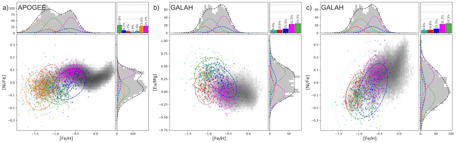
Figure 5: Distribution of GMM classified stars in APOGEE- & GALAH-Gaia sample in chemical dimensions ([Ni/Fe], [Eu/Mg]) that are not used in the GMM. Since [Ni/Fe] and [Eu/Mg] are not used in the GMM, the GMM result doesn’t contain the modelled mean, covariance, and $\sigma$ for these dimensions. Instead, we use the GMM classified member stars for each component and fit a Gaussian representing their distribution in each projection. This fit is marked with dashed line. The color schema follows the Figure 2 and 3. a): [Ni/Fe] vs [Fe/H] for APOGEE-Gaia sample, b): [Eu/Mg] vs [Fe/H] for GALAH-Gaia sample, c): [Mg/Cu] vs [Na/Fe] for GALAH-Gaia sample.

As far as the iron-peak elements are concerned, in particular those sensitive to SN Ia enrichment, as shown in Figure 5, there is a positive [Ni/Fe]–[Fe/H] correlation amongst Aurora’s stars. Interestingly this is a very different [Ni/Fe] trend compared to GS/E at a similar metallicity. Moreover a good number of Aurora stars sit above GS/E in [Ni/Fe]. At the same time, [Mn/Fe] shows no apparent difference (see Figure 4). As Sanders et al. (2021) discuss, the plane of [Ni/Fe] and [Mn/Fe] provides a way to decipher SN Ia yields and their dependence on e.g. the host’s star formation history. As Figure 9 of Sanders et al. (2021) shows, increased [Ni/Fe] at slowly varying metallicity and [Mn/Fe] may signal the growing contribution of massive SN Ia progenitors, which in turn may indicate a rise in star formation activity. Note that in massive Milky Way dwarfs [Ni/Fe] typically slowly decreases with metallicity, with the exception of the LMC where [Ni/Fe] shows an uptick connected to the most recent star formation burst (see Hasselquist et al., 2021).

Both [Eu/Fe] and [Eu/Mg] are markedly lower in Aurora compared to GS/E at the same metallicity (see Figures 4 and  5). Recently, Naidu et al. (2022) noticed a similar difference between the proposed Heracles stars and GS/E. Using indirect evidence for star formation timescale in the two populations, they concluded that Heracles must have had a shorter (faster) SF activity compared to GS/E. Naidu et al. (2022) then explained the increase in [Eu/Mg] by the delay in the neutron star merger (NSM) contribution to Eu production, where the early phases of the enrichment in this $r$-process element are driven mostly by core collapse SN (CCSN). Perhaps both the [Ni/Fe] and the [Eu/Mg] trends in Aurora’s stars are different pieces of evidence pointing in the direction of rapid SF activity in this ancient Milky Way population.

Comparing Aurora to Heracles (c.f. this work and those by Naidu et al., 2022; Horta et al., 2022), it appears that in all chemical dimensions these two populations are close to indistinguishable. Yet, the proposed origins of the two are very different. While Aurora is created in situ, Heracles is hypothesised to be an ancient merger event that occurred before the Milky Way-GS/E interaction. Heracles’ stellar debris typically occupy high-eccentricity orbits (eccentricity $>0.6$) but at a considerably lower energy range than the GS/E stars. Horta et al. (2021) used the apparent energy gap seen in the APOGEE dataset (see e.g., their Figure 4) to separate the GS/E and the Heracles stars. The Heracles’ chemical signature is also different from that of the GS/E, for example, its [Mg/Fe] level remains consistently high while at the same range of metallicity, the GS/E shows a clear $\alpha$-knee, i.e. a decreasing trend with [Fe/H]. Additionally, there have been two separate studies proposing the existence of another major merger in our Galaxy, which supposedly took place, like Heracles, before the GS/E event. Based on the age-metallicity and the number of globular clusters residing in the very centre of the Milky Way, Kruijssen et al. (2019) argued for a major merger with a massive galaxy they named Kraken; a similar merger (Koala) was suggested by Forbes (2020). As these studies all suggest an older massive merger event (occurring before GS/E) with its debris mostly populating the inner Galaxy, a consensus is starting to emerge in the literature that Kraken, Koala and Heracles are in fact the same event (see e.g., Naidu et al., 2022).

A recent study by Lane et al. (2022) (see e.g., their Section 6.3) pointed out that the dynamical characteristics of Heracles (e.g., the energy gap used to identify it as a distinct low-energy overdensity), is similar to the artificial density features induced by the APOGEE selection function. Indeed, no evidence for such an energy gap exists in the GALAH data which has a different (less bi-modal) selection function. Chemically, the low-[Fe/H], low-[Al/Fe] portion of Aurora is remarkably similar to Heracles. Both have high [Mg/Fe], high [Mg/Mn], [Eu/Mg] $\approx 0$ (c.f. this study and Naidu et al., 2022; Horta et al., 2022). The only strong difference involves [Al/Fe]: Aurora increases rapidly from sub-zero values (where it overlaps with Heracles) to extremely high [Al/Fe] $>0.5$ dex, while Heracles stars have [Al/Fe] $<0$ dex. Note however that the difference in [Al/Fe] between the two populations is artificial as the Heracles is selected to have negative [Al/Fe] to be consistent with an ex situ origin (Horta et al., 2021; Naidu et al., 2022; Horta et al., 2022). A more in-depth detailed analysis can be carried out by comparing the Aurora chemical properties as displayed in Figures 2,  3,  4 and  5 here to Heracles’ chemical fingerprint as shown in Horta et al. (2022). The similarities are striking. Despite being nearly identical chemically, Heracles and Aurora appear to occupy very different regions of the orbital energy (and consequently Galactocentric radius) distribution. Heracles is selected to have low energy and reside in the bulge, while Aurora has been identified - both here and in Belokurov & Kravtsov (2022) - outside of the bulge, amongst stars on high energy orbits. A comparison of the chemo-dynamical properties of Aurora and Heracles seem to indicate that this is the same population that is not bound to either inner or outer Galaxy. Instead, probably, it extends beyond the Solar neighborhood but is mostly concentrated in the bulge, similar to the numerical examples shown in Figure 12 of Belokurov & Kravtsov (2022).

4.5 Eos

The GMM reconstruction of the local halo populations has revealed a new eccentric component that we dub Eos. This previously unseen population occupies the metallicity range similar to that of Splash, i.e. $-1<$[Fe/H]$<-0.3$ dex. Eos, which is shown in blue in the Figures in this paper, contributes $\approx 10\%$ in APOGEE sample and $\approx 15\%$ in GALAH sample. What sets Eos apart is its relatively low $\alpha$-abundance level, it appears to be intermediate between the high-$\alpha$ sequence (in our sample represented by Splash) and the GS/E at similar metallicity. Note also the difference in the orbital energy between Eos and the high-$\alpha$ components (Aurora, Splash). Eos stars have relatively higher orbital energy implying that it populates larger (outer) Galactic radii.

At its highest metallicity, across all elements Eos connects seamlessly to the low-$\alpha$ (thin disk) sequence, yet unlike the disk it is highly eccentric. On the other hand, at its lowest metallicity Eos resembles more GS/E than any other Galactic stellar populations. This is particularly obvious in [Al/Fe], [Ce/Fe], [Na/Fe], [Eu/Fe], [Ni/Fe], [Eu/Fe] and [Eu/Mg]. Could Eos be a new accreted component of the halo? Judging by its high overall [Al/Fe], probably not. Its [Al/Fe] levels are higher than GS/E’s but not as high as the high-$\alpha$ population. Moreover, Eos exhibits a clear correlation between [Al/Fe] and [Fe/H] with a less steep slope compared to that of Aurora. The [Al/Fe] signature of Eos are replicated in the other odd-$z$ element available as part of this analysis, Na. Based on the elevated [Al/Fe] and [Na/Fe] values as well as their correlation with [Fe/H] we follow the ideas of Nissen & Schuster (2010) and Hawkins et al. (2015) and conclude that Eos was created in situ. As shown by Hasselquist et al. (2021) no Milky Way dwarf no matter how massive can reach as high levels of [Al/Fe] attained by the Eos.

Another interesting trend in Eos population is a possible bifurcation in [$\alpha$/Fe]–[Fe/H] plane visible in APOGEE sample (Figure 2, panel a) at around [Fe/H]$\approx-0.5$. A subset of Eos stars appear to form a branch between the higher-[$\alpha$/Fe] with higher-[Fe/H] and the lower-[$\alpha$/Fe] with lower-[Fe/H] region in the [$\alpha$/Fe]–[Fe/H] plane. These stars also show relatively higher [Al/Fe] abundances than the rest of Eos stars with comparable metallicity. This feature could be in line with the “Bridge” region suggested by Ciucă et al. (2021) as a transition region connecting the old thick (high-$\alpha$) and young thin (low-$\alpha$) disks, with a possible age gradient (older at higher [$\alpha$/Fe], younger at lower [$\alpha$/Fe]). This Bridge region doesn’t exactly overlap with Eos’s possible higher-$\alpha$ subbranch (Bridge region covers slightly higher metallicity and spans a very broad range of metallicity; see e.g., Figure 6 of Ciucă et al., 2021). Yet, the general idea of the transition signature running from higher-[$\alpha$/Fe] with higher-[Fe/H] to lower-[$\alpha$/Fe] with lower-[Fe/H] could be in line with Eos’s possible higher-[$\alpha$/Fe] subbranch feature, as a trace of gradual gas mixing (polluting) between the leftover gas from high-$\alpha$ (think) disk and the gas from GS/E merger (more discussion on Eos’s origin in Section 5.1). We should also consider the possible blending from GMM fitting between Eos and the high-$\alpha$ disk populations, as these higher-[$\alpha$/Fe] Eos stars are relatively closer to the high-$\alpha$ disk population in the chemical space.

Eos’s low-$\alpha$ abundance combined with its intermediate odd-Z abundance level also places Eos stars in a unique region of [Mg/Mn]–[Al/Fe] and [Mg/Cu]–[Na/Fe] planes (panel f) of Figures 2 and 3, panel c) of Figure 4). These planes have been successfully used to discern the less-evolved (and/or ex situ) and more-evolved (in situ) stellar populations. As a less evolved portion of the low-$\alpha$ in situ population, Eos appears between the region occupied by GS/E and the bulk of the low-$\alpha$ in situ stars (shown as a 2D density histogram in the Figures). Eos also sits below the region where Aurora is located in this plane emphasising a clear difference in their $\alpha$ abundance levels. Although both Eos and Aurora are likely to be the Galaxy’s in situ components, clear differences between them in a number of key elemental trends such as metallicity, $\alpha$, and odd-Z suggests different formation channels for Eos and Aurora. In several of the chemical projections Eos also displays a correlation with metallicity, i.e. [Mn/Fe], [Eu/Fe], [Ni/Fe], [Mg/Cu] all show trends with [Fe/H].

The chemical trajectory of Eos is unique, its chemical evolution appears to have started from the gas polluted by the GS/E and evolved into a typical low-alpha (thin disk) population.

5 Discussion and Summary

5.1 Clues to Eos’s origin

Deciphering the Eos’s origin may help us to solve the conundrum of the (trans)formation of the Milky Way’s disc. A part of the puzzle is the existence of a striking chemical bi-modality: two nearly parallel but well separated sequences are detected in the disc’s $\alpha$-[Fe/H] plane at a wide range of stellar metallicities and Galactocentric distances (e.g. Fuhrmann, 1998; Feltzing et al., 2003; Adibekyan et al., 2013; Bensby et al., 2014; Hayden et al., 2015). The high-$\alpha$ sequence and the low-$\alpha$ sequence have been linked to the so-called “thick” and “thin” discs respectively, although given the recent structural analysis it may be more appropriate to label the discs “inner” and “outer” (see e.g. Haywood et al., 2013; Rix & Bovy, 2013). Chronologically, the high-$\alpha$ and the low-$\alpha$ discs appear distinct: the former built up most of its mass before 8-10 Gyr ago, the epoch around which the first cinders of star-formation have been detected in the thin disc which has been growing steadily ever since (see e.g. Haywood et al., 2018a; Fantin et al., 2019).

Several scenarios have been proposed to explain the $\alpha$-dichotomy in the Galactic disc. For example, the “two-infall” model requires that in the distant past an episode of gas accretion diluted the Milky Way’s reservoir, resetting its metallicity so that the subsequent star-formation could proceed along the lower $\alpha$-sequence starting from a lowered value of [Fe/H] (see Chiappini et al., 1997; Chiappini, 2009; Grisoni et al., 2017). Alternatively, the observed $\alpha$-bimodality can be produced via radial migration and “churning” of the stars created along the two $\alpha$-sequences in distinct (broadly speaking, inner and outer) parts of the disc (see Sellwood & Binney, 2002; Roškar et al., 2008; Schönrich & Binney, 2009; Minchev et al., 2013). A new idea was proposed recently where the two spatially overlapping $\alpha$-sequences can start forming contemporaneously: massive dense gas clumps dominate the production of stars with high $\alpha$-abundance, while the smooth distributed star-formation is responsible for the low $\alpha$-abundance (Clarke et al., 2019). Finally, it is now also possible to form galaxies with $\alpha$-bimodal discs in Cosmological hydrodynamical simulations. Curiously, in the simulated discs, the $\alpha$-dichotomy is generally linked to ancient massive gas-rich accretion events (see e.g. Brook et al., 2012; Grand et al., 2018; Mackereth et al., 2018; Buck, 2020), however the details might vary. For example, in Agertz et al. (2021) around redshift z=1.5 a gas-rich accretion creates an outer low-$\alpha$ disc misaligned with respect to the earlier-formed inner high-$\alpha$ one; after a while, the two discs line up, leading to spatially overlapping low- and high-$\alpha$ stellar populations (see Renaud et al., 2021). In Grand et al. (2020), an analogue of the thick disc exists prior to the GS/E event but this violent interaction contributes to its additional heating; moreover, the gas-rich GS/E merger induces a star-burst in the central MW which adds between 20% and 60% stellar mass to the thick disc. As hinted by these recent studies based on cosmological hydrodynamical simulations, the Galactic discs and the GS/E event are linked in terms of their kinematics, chemical composition, and chronology.

Curiously, both Renaud et al. (2021) and Grand et al. (2020) discuss the emergence of an in situ halo-like population distinct from Splash and not much dissimilar to Eos around the time of the GS/E accretion. In Grand et al. (2020), a GS/E-like merger both splashes the pre-existing disk and induces a starburst in the centre of the Galaxy which leads to creation of a puffed-up halo-like in situ component. The simulated Splash would be expected to have a wide range of ages truncated around the time of the GS/E arrival, while the starburst population’s SFH would peak at the epoch of the interaction. In Renaud et al. (2021), the GS/E-like merger not only triggers star formation in the mis-aligned outer gaseous disk but also kick-starts its re-orienting with the pre-existing inner one. The two gas disks align rapidly but the first stars that were born in the outer disk are left behind in a strongly tilted configuration. The early outer disk stars subsequently phase-mix, and at the present day lack any appreciable angular momentum – the memory of their particular initial condition. The scenario of Renaud et al. (2021) is remarkable in that it predicts the existence of an in situ halo-like population with a narrow age distribution and the chemistry similar to the metal-poor low-$\alpha$ disk.

In the two-infall scenario, a variation of which is played out in the simulations discussed above, the re-setting of the disk’s chemical sequence is facilitated by the accretion of fresh, poorly-enriched gas from the medium around the host. It is also possible to directly invoke the accretion and recycling of the gas from the GS/E progenitor (see Grand et al., 2020; Palla et al., 2020). The dwarf is not required to donate its gas (which may not be enough to make a huge difference), it merely needs to enrich the gas surrounding the host. The exact amount of the heavy elements the dwarf can infuse into the condensing circumgalactic medium (CGM) will depend on the state of the gas and the parameters of the host-satellite interaction. Importantly, however, the mass loading factor of the pre-enriched outflows are predicted to be higher in the dwarf galaxy compared to the more massive host (Mitchell et al., 2020; Pandya et al., 2021). This is because the energetics at the feedback site do not depend on the host’s global properties, but the restoring force (gravity) does. This idea may have some support in the chemical properties of Eos. As Figures 2, 3 and 4 demonstrate, at its lowest metallicity, Eos is closest to the metal-rich portion of the GS/E sequence.

5.2 Caveats

Our study uses GMM to analyse unlabelled data in hyper-dimensional space consisting primarily of chemical information. Our modelling is based on the assumption that any sub-population found in the data follows a Gaussian distribution in the data space of choice. Unfortunately there is no guarantee that this is actually true. If a real physical trend in the data deviates severely from Gaussian distribution (e.g., a stellar population in [$\alpha$/Fe]–[Fe/H] with changing $\alpha$ abundance slope), this single stellar population can be segmented into multiple Gaussian components in the GMM fit. Any hard boundary cut applied to the data can also degrade the GMM performance. Therefore, we avoid the use of any dimension in our GMM if this dimension is directly used for any selection cuts adopted.

Populations seen in our sample are the high-eccentricity tails of their actual orbital distribution. For each population, this will bias the weight of the population assigned by the GMM depending on the degree of radial anisotropy. For example, Aurora is shown to be isotropic with its velocity dispersion, i.e., $\sigma_{\mathrm{R}}\approx\sigma_{\mathrm{z}}\approx\sigma_{\mathrm{\phi}}$ (see Belokurov & Kravtsov, 2022, for more detail). In contrast, GS/E or Splash are known for their strong radial anisotropy (e.g., Belokurov et al., 2018; Myeong et al., 2018c, d; Belokurov et al., 2020). Such a difference is reflected in their orbital eccentricity distribution, and different proportions of each population will be included in our high-eccentricity sample. While we have avoided making a cut on energy, the apocenter $>5$ kpc cut puts a slightly softer lower limit on the orbital energy range in our sample. This can bias the components’ properties if they are found near this lower energy boundary. For example, Aurora and Splash appear to extend down to the lowest energies, close to the limit imposed.

The reliability of chemical measurements varies with all of the atmospheric parameters and generally deteriorates towards the lower end of the metallicity range. To minimize the effect of varying uncertainty, we adopted the XD algorithm for our GMM which can take account of measurement errors associated with the observed data. However, of course, the systematic (unreported) errors will still affect the results of our modelling. The metallicity probed by both APOGEE and GALAH is truncated earlier as both surveys struggle in the low-[Fe/H] regime. The metallicity limit can also confuse the recovery of the true stellar populations in the data, especially for those components that extend far down in [Fe/H], e.g. GS/E and Aurora.

5.3 Summary

Our study provides one of the first attempt to assemble an unbiased census of the main halo components in the vicinity of the Sun. To carry out this experiment, we use the Extreme Deconvolution implementation of the Gaussian Mixture Model. To help the GMM concentrate on the stellar populations of interest, we apply an eccentricity cut thus limiting the sample to the halo stars only. The GMM model provides results that show consistency between APOGEE and GALAH in terms of the number and the properties of the components recovered. Moreover, when comparing the detailed properties of the individual components in APOGEE and GALAH we see clear consistency for the same chemical elements and for the same groups of elements (e.g. the [Al/Fe] behaviour is consistent with the [Na/Fe] behavior). Small differences in fractional contributions of the components between APOGEE and GALAH are likely due to the surveys’ distinct selection functions.

The reliability of the GMM decomposition reported here can be established by comparing the chemical properties of the known and well-studied halo components to those reported in the literature. For example, our view of the GS/E chemical fingerprint is in full agreement with the recent studies (see e.g. Das et al., 2020; Hasselquist et al., 2021; Buder et al., 2021b; Aguado et al., 2021a; Matsuno et al., 2021; Naidu et al., 2022; Horta et al., 2022; Carrillo et al., 2022). Similarly, we demonstrate that across all chemical dimensions investigated, Splash is indistinguishable from the high-$\alpha$ (thick disk) of the Milky Way. This is of course in agreement with the proposed origin of this in situ halo population (see e.g Bonaca et al., 2017; Haywood et al., 2018b; Gallart et al., 2019; Di Matteo et al., 2019; Belokurov et al., 2020).

While it is reassuring to see agreement between the earlier attempts to decipher the chemical behavior of the halo denizens and our unsupervised analysis, the results of this work are not limited to mere confirmation. Let us summarise the most interesting new findings here.

• The GMM finds only four independent halo components dominating the Solar neighborhood, three of these are previously known, i.e. Aurora, Splash and GS/E, and one is new. There is strong evidence that the newly discovered population Eos is of in situ origin. Therefore, in the Solar neighbourhood, our analysis detects no evidence for tidal debris from any additional large accretion event.

• As reported by the GMM, the multi-dimensional chemical view of the ancient in situ component Aurora (see Belokurov & Kravtsov, 2022) agrees remarkably well with the chemical properties of the alleged merger remnant known as Heracles (Horta et al., 2021; Naidu et al., 2022; Horta et al., 2022). The only noticeable difference appears to stem from the fact that in the literature the Heracles stars are identified using a hard-cut in [Al/Fe] while here we dispense with selections in the chemical space. Our study preserves the integrity of the stellar populations in the elemental abundance space and demonstrates that in [Al/Fe]–[Fe/H] dimension Aurora evolves rapidly from low [Al/Fe] to anomalously high [Al/Fe]. This behaviour is predicted for a rapidly star-forming self-enriching galaxy with a mass similar to that of the Milky Way (see Horta et al., 2021) and thus obviates the necessity for introducing an additional merger event to explain this stellar population.

• The chemical properties of the discovered in situ born structure Eos evolve significantly as a function of metallicity. At its lowest [Fe/H] Eos does not resemble any of the known in situ populations, especially those that are predicted to have formed early, i.e. Aurora or Splash. Instead, the low-[Fe/H] Eos’s stars look similar to the most metal-rich GS/E members. However, at its highest [Fe/H] Eos connects seamlessly to the chemical sequence of the low-$\alpha$ (thin disk) stars. This strong evolution is exhibited as clear correlation between e.g. [Al/Fe], [Mn/Fe], [Eu/Fe], [Ni/Fe] and [Fe/H]. We speculate that Eos appears to originate from the gas polluted by the GS/E and evolved to resemble the (outer) thin disk of the Milky Way.

The unsupervised view of the local halo the GMM provides also allows us to decipher many new and fine details of the four components detected. For example, in APOGEE, the GS/E is split into two components that primarily differ in metallicity but trace distinct epochs in the life of the progenitor galaxy, i.e. one corresponding to the high-$\alpha$ plateau and slowly rising [Al/Fe] and another to the knee/decline in $\alpha$ and in [Al/Fe] due to the increased SN Ia contribution. We also see that the two GS/E components behave differently in Ni (iron-peak element particularly sensitive to variations in SN Ia yields). Curiously, the GS/E trends in [Ni/Fe]–[Fe/H] space are distinct from that of Aurora at similar metallicity. In both APOGEE and GALAH, Aurora attains the highest abundance ratios in $\alpha$, [Al/Fe], [Ce/Fe], [Y/Fe], [Ba/Fe], [Ba/Eu] of all 4 components. Moreover, it shows strong correlations between [Ce/Fe], [Al/Fe], [Y/Fe], [Ba/Fe] and [Fe/H]. We interpret such behaviour as additional evidence that massive star clusters may have contributed significantly to the chemical evolution of Aurora (as argued in Belokurov & Kravtsov, 2022). We note that Aurora has significantly lower [Eu/Fe] and [Eu/Mg] compared to GS/E at similar metallicity, the trend that has been claimed previously for Heracles by Naidu et al. (2021).

Deciphering the origin of Eos with the help of numerical simulations, both those currently available such as FIRE (Hopkins et al., 2014), Auriga (Grand et al., 2017), VINTERGATAN (Agertz et al., 2021) and ARTEMIS (Font et al., 2020), as well as those upcoming, is the obvious next step. Currently the feedback physics remains somewhat unconstrained but there may be routes to test the proposed formation mechanism of Eos, in particular, the role of the GS/E progenitor galaxy in the pollution of the circum-host gas and the triggering of the in situ star formation. The (relative) stellar ages (see e.g. Conroy et al., 2022; Xiang & Rix, 2022) also provide valuable information and will help to expand the current analysis to a chrono-chemo-dynamical study. Undoubtedly, detailed information from the upcoming large spectroscopic surveys (e.g., DESI, 4MOST, WEAVE, SDSS-V) and astrometric surveys (e.g., Gaia, LSST) will open up new arenas for decoding the genealogy of the Galaxy.

References

- Abdurro’uf et al. (2022) Abdurro’uf, Accetta, K., Aerts, C., et al. 2022, ApJS, 259, 35, doi: 10.3847/1538-4365/ac4414
- Adibekyan et al. (2013) Adibekyan, V. Z., Figueira, P., Santos, N. C., et al. 2013, A&A, 554, A44, doi: 10.1051/0004-6361/201321520
- Agertz et al. (2021) Agertz, O., Renaud, F., Feltzing, S., et al. 2021, MNRAS, 503, 5826, doi: 10.1093/mnras/stab322
- Aguado et al. (2021a) Aguado, D. S., Belokurov, V., Myeong, G. C., et al. 2021a, ApJ, 908, L8, doi: 10.3847/2041-8213/abdbb8
- Aguado et al. (2021b) Aguado, D. S., Myeong, G. C., Belokurov, V., et al. 2021b, MNRAS, 500, 889, doi: 10.1093/mnras/staa3250
- Akaike (1974) Akaike, H. 1974, IEEE Transactions on Automatic Control, 19, 716, doi: 10.1109/TAC.1974.1100705
- Alencastro Puls et al. (2022) Alencastro Puls, A., Casagrande, L., Monty, S., et al. 2022, MNRAS, 510, 1733, doi: 10.1093/mnras/stab3545
- Astropy Collaboration et al. (2013) Astropy Collaboration, Robitaille, T. P., Tollerud, E. J., et al. 2013, A&A, 558, A33, doi: 10.1051/0004-6361/201322068
- Astropy Collaboration et al. (2018) Astropy Collaboration, Price-Whelan, A. M., Sipőcz, B. M., et al. 2018, AJ, 156, 123, doi: 10.3847/1538-3881/aabc4f
- Bailer-Jones et al. (2021) Bailer-Jones, C. A. L., Rybizki, J., Fouesneau, M., Demleitner, M., & Andrae, R. 2021, AJ, 161, 147, doi: 10.3847/1538-3881/abd806
- Balbinot & Helmi (2021) Balbinot, E., & Helmi, A. 2021, A&A, 654, A15, doi: 10.1051/0004-6361/202141015
- Belokurov et al. (2018) Belokurov, V., Erkal, D., Evans, N. W., Koposov, S. E., & Deason, A. J. 2018, MNRAS, 478, 611, doi: 10.1093/mnras/sty982
- Belokurov & Kravtsov (2022) Belokurov, V., & Kravtsov, A. 2022, arXiv e-prints, arXiv:2203.04980. https://arxiv.org/abs/2203.04980
- Belokurov et al. (2020) Belokurov, V., Sanders, J. L., Fattahi, A., et al. 2020, MNRAS, 494, 3880, doi: 10.1093/mnras/staa876
- Bensby et al. (2014) Bensby, T., Feltzing, S., & Oey, M. S. 2014, A&A, 562, A71, doi: 10.1051/0004-6361/201322631
- Bignone et al. (2019) Bignone, L. A., Helmi, A., & Tissera, P. B. 2019, ApJ, 883, L5, doi: 10.3847/2041-8213/ab3e0e
- Bird et al. (2021) Bird, S. A., Xue, X.-X., Liu, C., et al. 2021, ApJ, 919, 66, doi: 10.3847/1538-4357/abfa9e
- Bonaca et al. (2017) Bonaca, A., Conroy, C., Wetzel, A., Hopkins, P. F., & Kereš, D. 2017, ApJ, 845, 101, doi: 10.3847/1538-4357/aa7d0c
- Bonaca et al. (2020) Bonaca, A., Conroy, C., Cargile, P. A., et al. 2020, ApJ, 897, L18, doi: 10.3847/2041-8213/ab9caa
- Bonifacio et al. (2021) Bonifacio, P., Monaco, L., Salvadori, S., et al. 2021, A&A, 651, A79, doi: 10.1051/0004-6361/202140816
- Borsato et al. (2020) Borsato, N. W., Martell, S. L., & Simpson, J. D. 2020, MNRAS, 492, 1370, doi: 10.1093/mnras/stz3479
- Bovy (2015) Bovy, J. 2015, ApJS, 216, 29, doi: 10.1088/0067-0049/216/2/29
- Bovy et al. (2011) Bovy, J., Hogg, D. W., & Roweis, S. T. 2011, Annals of Applied Statistics, 5, 1657, doi: 10.1214/10-AOAS439
- Brook et al. (2003) Brook, C. B., Kawata, D., Gibson, B. K., & Flynn, C. 2003, ApJ, 585, L125, doi: 10.1086/374306
- Brook et al. (2012) Brook, C. B., Stinson, G. S., Gibson, B. K., et al. 2012, MNRAS, 426, 690, doi: 10.1111/j.1365-2966.2012.21738.x
- Buck (2020) Buck, T. 2020, MNRAS, 491, 5435, doi: 10.1093/mnras/stz3289
- Buder et al. (2021a) Buder, S., Sharma, S., Kos, J., et al. 2021a, MNRAS, 506, 150, doi: 10.1093/mnras/stab1242
- Buder et al. (2021b) Buder, S., Lind, K., Ness, M. K., et al. 2021b, arXiv e-prints, arXiv:2109.04059. https://arxiv.org/abs/2109.04059
- Callingham et al. (2022) Callingham, T. M., Cautun, M., Deason, A. J., et al. 2022, MNRAS, 513, 4107, doi: 10.1093/mnras/stac1145
- Carollo & Chiba (2021) Carollo, D., & Chiba, M. 2021, ApJ, 908, 191, doi: 10.3847/1538-4357/abd7a4
- Carrillo et al. (2022) Carrillo, A., Hawkins, K., Jofré, P., et al. 2022, MNRAS, doi: 10.1093/mnras/stac518
- Chiappini (2009) Chiappini, C. 2009, in The Galaxy Disk in Cosmological Context, ed. J. Andersen, Nordströara, B. m, & J. Bland-Hawthorn, Vol. 254, 191–196, doi: 10.1017/S1743921308027580
- Chiappini et al. (1997) Chiappini, C., Matteucci, F., & Gratton, R. 1997, ApJ, 477, 765, doi: 10.1086/303726
- Chiba & Yoshii (1998) Chiba, M., & Yoshii, Y. 1998, AJ, 115, 168, doi: 10.1086/300177
- Ciucă et al. (2021) Ciucă, I., Kawata, D., Miglio, A., Davies, G. R., & Grand, R. J. J. 2021, MNRAS, 503, 2814, doi: 10.1093/mnras/stab639
- Clarke et al. (2019) Clarke, A. J., Debattista, V. P., Nidever, D. L., et al. 2019, MNRAS, 484, 3476, doi: 10.1093/mnras/stz104
- Conroy et al. (2022) Conroy, C., Weinberg, D. H., Naidu, R. P., et al. 2022, arXiv e-prints, arXiv:2204.02989. https://arxiv.org/abs/2204.02989
- Das et al. (2020) Das, P., Hawkins, K., & Jofré, P. 2020, MNRAS, 493, 5195, doi: 10.1093/mnras/stz3537
- Deason et al. (2011) Deason, A. J., Belokurov, V., & Evans, N. W. 2011, MNRAS, 416, 2903, doi: 10.1111/j.1365-2966.2011.19237.x
- Deason et al. (2013) Deason, A. J., Belokurov, V., Evans, N. W., & Johnston, K. V. 2013, ApJ, 763, 113, doi: 10.1088/0004-637X/763/2/113
- Deason et al. (2018) Deason, A. J., Belokurov, V., Koposov, S. E., & Lancaster, L. 2018, ApJ, 862, L1, doi: 10.3847/2041-8213/aad0ee
- Deason et al. (2019) Deason, A. J., Belokurov, V., & Sanders, J. L. 2019, MNRAS, 490, 3426, doi: 10.1093/mnras/stz2793
- Di Matteo et al. (2019) Di Matteo, P., Haywood, M., Lehnert, M. D., et al. 2019, A&A, 632, A4, doi: 10.1051/0004-6361/201834929
- Dillamore et al. (2022) Dillamore, A. M., Belokurov, V., Font, A. S., & McCarthy, I. G. 2022, MNRAS, 513, 1867, doi: 10.1093/mnras/stac1038
- D’Onghia et al. (2009) D’Onghia, E., Besla, G., Cox, T. J., & Hernquist, L. 2009, Nature, 460, 605, doi: 10.1038/nature08215
- Elias et al. (2020) Elias, L. M., Sales, L. V., Helmi, A., & Hernquist, L. 2020, MNRAS, 495, 29, doi: 10.1093/mnras/staa1090
- Erkal et al. (2019) Erkal, D., Belokurov, V., Laporte, C. F. P., et al. 2019, MNRAS, 487, 2685, doi: 10.1093/mnras/stz1371
- Evans (2020) Evans, N. W. 2020, in Galactic Dynamics in the Era of Large Surveys, ed. M. Valluri & J. A. Sellwood, Vol. 353, 113–120, doi: 10.1017/S1743921319009700
- Evans et al. (2019) Evans, N. W., O’Hare, C. A. J., & McCabe, C. 2019, Phys. Rev. D, 99, 023012, doi: 10.1103/PhysRevD.99.023012
- Fantin et al. (2019) Fantin, N. J., Côté, P., McConnachie, A. W., et al. 2019, ApJ, 887, 148, doi: 10.3847/1538-4357/ab5521
- Fantin et al. (2021) —. 2021, ApJ, 913, 30, doi: 10.3847/1538-4357/abf2b2
- Fattahi et al. (2019) Fattahi, A., Belokurov, V., Deason, A. J., et al. 2019, MNRAS, 484, 4471, doi: 10.1093/mnras/stz159
- Feltzing et al. (2003) Feltzing, S., Bensby, T., & Lundström, I. 2003, A&A, 397, L1, doi: 10.1051/0004-6361:20021661
- Fernández-Alvar et al. (2018) Fernández-Alvar, E., Carigi, L., Schuster, W. J., et al. 2018, ApJ, 852, 50, doi: 10.3847/1538-4357/aa9ced
- Feuillet et al. (2020) Feuillet, D. K., Feltzing, S., Sahlholdt, C. L., & Casagrande, L. 2020, MNRAS, 497, 109, doi: 10.1093/mnras/staa1888
- Feuillet et al. (2019) Feuillet, D. K., Frankel, N., Lind, K., et al. 2019, MNRAS, 489, 1742, doi: 10.1093/mnras/stz2221
- Feuillet et al. (2021) Feuillet, D. K., Sahlholdt, C. L., Feltzing, S., & Casagrande, L. 2021, MNRAS, 508, 1489, doi: 10.1093/mnras/stab2614
- Font et al. (2020) Font, A. S., McCarthy, I. G., Poole-Mckenzie, R., et al. 2020, MNRAS, 498, 1765, doi: 10.1093/mnras/staa2463
- Forbes (2020) Forbes, D. A. 2020, MNRAS, 493, 847, doi: 10.1093/mnras/staa245
- Frankel et al. (2020) Frankel, N., Sanders, J., Ting, Y.-S., & Rix, H.-W. 2020, ApJ, 896, 15, doi: 10.3847/1538-4357/ab910c
- Fuhrmann (1998) Fuhrmann, K. 1998, A&A, 338, 161
- Gaia Collaboration et al. (2021) Gaia Collaboration, Brown, A. G. A., Vallenari, A., et al. 2021, A&A, 649, A1, doi: 10.1051/0004-6361/202039657
- Gallart et al. (2019) Gallart, C., Bernard, E. J., Brook, C. B., et al. 2019, Nature Astronomy, 3, 932, doi: 10.1038/s41550-019-0829-5
- Gelman et al. (2015) Gelman, A., Carlin, J., Stern, H., et al. 2015, Bayesian Data Analysis, 3rd edn. (Chapman and Hall)
- Gibbons et al. (2017) Gibbons, S. L. J., Belokurov, V., & Evans, N. W. 2017, MNRAS, 464, 794, doi: 10.1093/mnras/stw2328
- Grand et al. (2017) Grand, R. J. J., Gómez, F. A., Marinacci, F., et al. 2017, MNRAS, 467, 179, doi: 10.1093/mnras/stx071
- Grand et al. (2018) Grand, R. J. J., Bustamante, S., Gómez, F. A., et al. 2018, MNRAS, 474, 3629, doi: 10.1093/mnras/stx3025
- Grand et al. (2020) Grand, R. J. J., Kawata, D., Belokurov, V., et al. 2020, MNRAS, 497, 1603, doi: 10.1093/mnras/staa2057
- Grisoni et al. (2017) Grisoni, V., Spitoni, E., Matteucci, F., et al. 2017, MNRAS, 472, 3637, doi: 10.1093/mnras/stx2201
- Grunblatt et al. (2021) Grunblatt, S. K., Zinn, J. C., Price-Whelan, A. M., et al. 2021, ApJ, 916, 88, doi: 10.3847/1538-4357/ac0532
- Hasselquist et al. (2021) Hasselquist, S., Hayes, C. R., Lian, J., et al. 2021, ApJ, 923, 172, doi: 10.3847/1538-4357/ac25f9
- Hawkins et al. (2015) Hawkins, K., Jofré, P., Masseron, T., & Gilmore, G. 2015, MNRAS, 453, 758, doi: 10.1093/mnras/stv1586
- Hayden et al. (2015) Hayden, M. R., Bovy, J., Holtzman, J. A., et al. 2015, ApJ, 808, 132, doi: 10.1088/0004-637X/808/2/132
- Haywood et al. (2018a) Haywood, M., Di Matteo, P., Lehnert, M., et al. 2018a, A&A, 618, A78, doi: 10.1051/0004-6361/201731363
- Haywood et al. (2013) Haywood, M., Di Matteo, P., Lehnert, M. D., Katz, D., & Gómez, A. 2013, A&A, 560, A109, doi: 10.1051/0004-6361/201321397
- Haywood et al. (2018b) Haywood, M., Di Matteo, P., Lehnert, M. D., et al. 2018b, ApJ, 863, 113, doi: 10.3847/1538-4357/aad235
- Helmi et al. (2018) Helmi, A., Babusiaux, C., Koppelman, H. H., et al. 2018, Nature, 563, 85, doi: 10.1038/s41586-018-0625-x
- Helmi et al. (1999) Helmi, A., White, S. D. M., de Zeeuw, P. T., & Zhao, H. 1999, Nature, 402, 53, doi: 10.1038/46980
- Hopkins et al. (2014) Hopkins, P. F., Kereš, D., Oñorbe, J., et al. 2014, MNRAS, 445, 581, doi: 10.1093/mnras/stu1738
- Horta et al. (2021) Horta, D., Schiavon, R. P., Mackereth, J. T., et al. 2021, MNRAS, 500, 1385, doi: 10.1093/mnras/staa2987
- Horta et al. (2022) —. 2022, arXiv e-prints, arXiv:2204.04233. https://arxiv.org/abs/2204.04233
- Ibata et al. (2021) Ibata, R., Malhan, K., Martin, N., et al. 2021, ApJ, 914, 123, doi: 10.3847/1538-4357/abfcc2
- Ibata et al. (1994) Ibata, R. A., Gilmore, G., & Irwin, M. J. 1994, Nature, 370, 194, doi: 10.1038/370194a0
- Ibata et al. (2019) Ibata, R. A., Malhan, K., & Martin, N. F. 2019, ApJ, 872, 152, doi: 10.3847/1538-4357/ab0080
- Iorio & Belokurov (2019) Iorio, G., & Belokurov, V. 2019, MNRAS, 482, 3868, doi: 10.1093/mnras/sty2806
- Iorio & Belokurov (2021) —. 2021, MNRAS, 502, 5686, doi: 10.1093/mnras/stab005
- Kirby et al. (2013) Kirby, E. N., Cohen, J. G., Guhathakurta, P., et al. 2013, ApJ, 779, 102, doi: 10.1088/0004-637X/779/2/102
- Kobayashi et al. (2020) Kobayashi, C., Karakas, A. I., & Lugaro, M. 2020, ApJ, 900, 179, doi: 10.3847/1538-4357/abae65
- Koppelman et al. (2019) Koppelman, H. H., Helmi, A., Massari, D., Price-Whelan, A. M., & Starkenburg, T. K. 2019, A&A, 631, L9, doi: 10.1051/0004-6361/201936738
- Kordopatis et al. (2020) Kordopatis, G., Recio-Blanco, A., Schultheis, M., & Hill, V. 2020, A&A, 643, A69, doi: 10.1051/0004-6361/202038686
- Kruijssen et al. (2019) Kruijssen, J. M. D., Pfeffer, J. L., Reina-Campos, M., Crain, R. A., & Bastian, N. 2019, MNRAS, 486, 3180, doi: 10.1093/mnras/sty1609
- Lancaster et al. (2019) Lancaster, L., Koposov, S. E., Belokurov, V., Evans, N. W., & Deason, A. J. 2019, MNRAS, 486, 378, doi: 10.1093/mnras/stz853
- Lane et al. (2022) Lane, J. M. M., Bovy, J., & Mackereth, J. T. 2022, MNRAS, 510, 5119, doi: 10.1093/mnras/stab3755
- Limberg et al. (2021) Limberg, G., Rossi, S., Beers, T. C., et al. 2021, ApJ, 907, 10, doi: 10.3847/1538-4357/abcb87
- Loebman et al. (2011) Loebman, S. R., Roškar, R., Debattista, V. P., et al. 2011, ApJ, 737, 8, doi: 10.1088/0004-637X/737/1/8
- Mackereth & Bovy (2020) Mackereth, J. T., & Bovy, J. 2020, MNRAS, 492, 3631, doi: 10.1093/mnras/staa047
- Mackereth et al. (2018) Mackereth, J. T., Crain, R. A., Schiavon, R. P., et al. 2018, MNRAS, 477, 5072, doi: 10.1093/mnras/sty972
- Mackereth et al. (2019) Mackereth, J. T., Schiavon, R. P., Pfeffer, J., et al. 2019, MNRAS, 482, 3426, doi: 10.1093/mnras/sty2955
- Majewski et al. (2003) Majewski, S. R., Skrutskie, M. F., Weinberg, M. D., & Ostheimer, J. C. 2003, ApJ, 599, 1082, doi: 10.1086/379504
- Malhan et al. (2018) Malhan, K., Ibata, R. A., & Martin, N. F. 2018, MNRAS, 481, 3442, doi: 10.1093/mnras/sty2474
- Marino et al. (2009) Marino, A. F., Milone, A. P., Piotto, G., et al. 2009, A&A, 505, 1099, doi: 10.1051/0004-6361/200911827
- Massari et al. (2019) Massari, D., Koppelman, H. H., & Helmi, A. 2019, A&A, 630, L4, doi: 10.1051/0004-6361/201936135
- Mathewson et al. (1974) Mathewson, D. S., Cleary, M. N., & Murray, J. D. 1974, ApJ, 190, 291, doi: 10.1086/152875
- Matsuno et al. (2019) Matsuno, T., Aoki, W., & Suda, T. 2019, ApJ, 874, L35, doi: 10.3847/2041-8213/ab0ec0
- Matsuno et al. (2021) Matsuno, T., Hirai, Y., Tarumi, Y., et al. 2021, A&A, 650, A110, doi: 10.1051/0004-6361/202040227
- McMillan (2017) McMillan, P. J. 2017, MNRAS, 465, 76, doi: 10.1093/mnras/stw2759
- Mészáros et al. (2020) Mészáros, S., Masseron, T., García-Hernández, D. A., et al. 2020, MNRAS, 492, 1641, doi: 10.1093/mnras/stz3496
- Meza et al. (2005) Meza, A., Navarro, J. F., Abadi, M. G., & Steinmetz, M. 2005, MNRAS, 359, 93, doi: 10.1111/j.1365-2966.2005.08869.x
- Minchev et al. (2013) Minchev, I., Chiappini, C., & Martig, M. 2013, A&A, 558, A9, doi: 10.1051/0004-6361/201220189
- Mitchell et al. (2020) Mitchell, P. D., Schaye, J., Bower, R. G., & Crain, R. A. 2020, MNRAS, 494, 3971, doi: 10.1093/mnras/staa938
- Molaro et al. (2020) Molaro, P., Cescutti, G., & Fu, X. 2020, MNRAS, 496, 2902, doi: 10.1093/mnras/staa1653
- Montalbán et al. (2021) Montalbán, J., Mackereth, J. T., Miglio, A., et al. 2021, Nature Astronomy, 5, 640, doi: 10.1038/s41550-021-01347-7
- Monty et al. (2020) Monty, S., Venn, K. A., Lane, J. M. M., Lokhorst, D., & Yong, D. 2020, MNRAS, 497, 1236, doi: 10.1093/mnras/staa1995
- Myeong et al. (2018a) Myeong, G. C., Evans, N. W., Belokurov, V., Amorisco, N. C., & Koposov, S. E. 2018a, MNRAS, 475, 1537, doi: 10.1093/mnras/stx3262
- Myeong et al. (2018b) Myeong, G. C., Evans, N. W., Belokurov, V., Sanders, J. L., & Koposov, S. E. 2018b, MNRAS, 478, 5449, doi: 10.1093/mnras/sty1403
- Myeong et al. (2018c) —. 2018c, ApJ, 856, L26, doi: 10.3847/2041-8213/aab613
- Myeong et al. (2018d) —. 2018d, ApJ, 863, L28, doi: 10.3847/2041-8213/aad7f7
- Myeong et al. (2019) Myeong, G. C., Vasiliev, E., Iorio, G., Evans, N. W., & Belokurov, V. 2019, MNRAS, 488, 1235, doi: 10.1093/mnras/stz1770
- Naidu et al. (2020) Naidu, R. P., Conroy, C., Bonaca, A., et al. 2020, ApJ, 901, 48, doi: 10.3847/1538-4357/abaef4
- Naidu et al. (2021) —. 2021, ApJ, 923, 92, doi: 10.3847/1538-4357/ac2d2d
- Naidu et al. (2022) Naidu, R. P., Ji, A. P., Conroy, C., et al. 2022, ApJ, 926, L36, doi: 10.3847/2041-8213/ac5589
- Necib et al. (2019) Necib, L., Lisanti, M., & Belokurov, V. 2019, ApJ, 874, 3, doi: 10.3847/1538-4357/ab095b
- Nissen & Schuster (2010) Nissen, P. E., & Schuster, W. J. 2010, A&A, 511, L10, doi: 10.1051/0004-6361/200913877
- O’Hare et al. (2020) O’Hare, C. A. J., Evans, N. W., McCabe, C., Myeong, G., & Belokurov, V. 2020, Phys. Rev. D, 101, 023006, doi: 10.1103/PhysRevD.101.023006
- Palau & Miralda-Escudé (2019) Palau, C. G., & Miralda-Escudé, J. 2019, MNRAS, 488, 1535, doi: 10.1093/mnras/stz1790
- Palla et al. (2020) Palla, M., Matteucci, F., Spitoni, E., Vincenzo, F., & Grisoni, V. 2020, MNRAS, 498, 1710, doi: 10.1093/mnras/staa2437
- Pandya et al. (2021) Pandya, V., Fielding, D. B., Anglés-Alcázar, D., et al. 2021, MNRAS, 508, 2979, doi: 10.1093/mnras/stab2714
- Pedregosa et al. (2011) Pedregosa, F., Varoquaux, G., Gramfort, A., et al. 2011, Journal of Machine Learning Research, 12, 2825
- Renaud et al. (2021) Renaud, F., Agertz, O., Andersson, E. P., et al. 2021, MNRAS, 503, 5868, doi: 10.1093/mnras/stab543
- Rix & Bovy (2013) Rix, H.-W., & Bovy, J. 2013, A&A Rev., 21, 61, doi: 10.1007/s00159-013-0061-8
- Roškar et al. (2008) Roškar, R., Debattista, V. P., Stinson, G. S., et al. 2008, ApJ, 675, L65, doi: 10.1086/586734
- Sahlholdt et al. (2019) Sahlholdt, C. L., Casagrande, L., & Feltzing, S. 2019, ApJ, 881, L10, doi: 10.3847/2041-8213/ab321e
- Sanders et al. (2021) Sanders, J. L., Belokurov, V., & Man, K. T. F. 2021, MNRAS, 506, 4321, doi: 10.1093/mnras/stab1951
- Schönrich & Binney (2009) Schönrich, R., & Binney, J. 2009, MNRAS, 396, 203, doi: 10.1111/j.1365-2966.2009.14750.x
- Schwarz (1978) Schwarz, G. 1978, The Annals of Statistics, 6, 461 , doi: 10.1214/aos/1176344136
- Sellwood & Binney (2002) Sellwood, J. A., & Binney, J. J. 2002, MNRAS, 336, 785, doi: 10.1046/j.1365-8711.2002.05806.x
- Sharma et al. (2018) Sharma, S., Stello, D., Buder, S., et al. 2018, MNRAS, 473, 2004, doi: 10.1093/mnras/stx2582
- Simion et al. (2019) Simion, I. T., Belokurov, V., & Koposov, S. E. 2019, MNRAS, 482, 921, doi: 10.1093/mnras/sty2744
- Sofie Lövdal et al. (2022) Sofie Lövdal, S., Ruiz-Lara, T., Koppelman, H. H., et al. 2022, arXiv e-prints, arXiv:2201.02404. https://arxiv.org/abs/2201.02404
- Vasiliev (2019) Vasiliev, E. 2019, MNRAS, 482, 1525, doi: 10.1093/mnras/sty2672
- Vasiliev et al. (2022) Vasiliev, E., Belokurov, V., & Evans, N. W. 2022, ApJ, 926, 203, doi: 10.3847/1538-4357/ac4fbc
- Vincenzo et al. (2019) Vincenzo, F., Spitoni, E., Calura, F., et al. 2019, MNRAS, 487, L47, doi: 10.1093/mnrasl/slz070
- Wannier & Wrixon (1972) Wannier, P., & Wrixon, G. T. 1972, ApJ, 173, L119, doi: 10.1086/180930
- Wu et al. (2022) Wu, W., Zhao, G., Xue, X.-X., Bird, S. A., & Yang, C. 2022, ApJ, 924, 23, doi: 10.3847/1538-4357/ac31ac
- Xiang & Rix (2022) Xiang, M., & Rix, H.-W. 2022, Nature, 603, 599, doi: 10.1038/s41586-022-04496-5
- Yuan et al. (2020) Yuan, Z., Myeong, G. C., Beers, T. C., et al. 2020, ApJ, 891, 39, doi: 10.3847/1538-4357/ab6ef7