Improving Diversity with Adversarially Learned Transformations
for Domain Generalization

Abstract

To be successful in single source domain generalization (SSDG), maximizing diversity of synthesized domains has emerged as one of the most effective strategies. Recent success in SSDG comes from methods that pre-specify diversity inducing image augmentations during training, so that it may lead to better generalization on new domains. However, naïve pre-specified augmentations are not always effective, either because they cannot model large domain shift, or because the specific choice of transforms may not cover the types of shift commonly occurring in domain generalization. To address this issue, we present a novel framework called ALT: adversarially learned transformations, that uses an adversary neural network to model plausible, yet hard image transformations that fool the classifier. ALT learns image transformations by randomly initializing the adversary network for each batch and optimizing it for a fixed number of steps to maximize classification error. The classifier is trained by enforcing a consistency between its predictions on the clean and transformed images. With extensive empirical analysis, we find that this new form of adversarial transformations achieves both objectives of diversity and hardness simultaneously, outperforming all existing techniques on competitive benchmarks for SSDG. We also show that ALT can seamlessly work with existing diversity modules to produce highly distinct, and large transformations of the source domain leading to state-of-the-art performance. Code: https://github.com/tejas-gokhale/ALT

1 Introduction

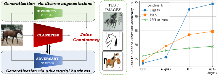
Figure 1: ALT consists of a diversity module (data augmentation functions such as Augmix [22] or RandConv [43] and an adversary network (to learn image transformations that fool the classifier). We show an example from the PACS benchmark under the single-source domain generalization setting, with real photos (P) as the source domain and art paintings (A), cartoons (C), and sketches (S) as the target domains. The plot summarizes our results – while diversity alone improves performance over the naive ERM baseline, adapting this diversity using adversarially learned transformations (ALT) provides a significant boost for domain generalization on multiple benchmarks.

Domain generalization is the problem of making accurate predictions on previously unseen domains, especially when these domains are very different from the data distribution on which the model was trained. This is a challenging problem that has seen steady progress over the last few years [4, 41, 33, 43, 31]. This paper focuses on the special case – single source domain generalization (SSDG) – where the model has access only to a single training domain, and is expected to generalize to multiple different testing domains. This is especially hard because of the limited information available to train the model with just a single source.

When multiple source domains are available (MSDG), recent analysis [18] shows that even simple methods like minimizing empirical risk jointly on all domains, performs better than most existing sophisticated formulations. A corollary to this finding is that success in DG is dependent on diversity – i.e., exposing the model to as many potential training domains as possible. As the SSDG problem allows access only to a single training domain, such an exposure must come in the form of diverse transformations of the source domain that can simulate the presence of multiple domains, ultimately leading to low generalization error.

The idea of using diversity to train models has been sufficiently explored – [22, 45, 46, 7] show that a diverse set of augmentations during training improves a model’s robustness under distribution shifts. Specific augmentations can be used if the type of diversity encountered at test time is known; for eg., if it is known that the test set contains random combinations of rotation, translation, and scaling, using augmentations correlated with this domain shift would lead to good performance [2, 42, 16]. However, since we cannot assume knowledge of the test domain under the SSDG problem statement, the extent to which the model needs to be exposed to specific augmentations remains unclear. Augmentation methods impose a strong prior in terms of the types of diversity that the model is exposed to, which may not match with desirable test-time transformations. As we will show in this paper, data augmentation methods that produce good results on one dataset, do not necessarily work on other datasets – in some cases, they may even hurt performance!

In addition to such a knowledge gap, unfortunately, such augmentation methods can only achieve invariance under small distribution shifts like unknown corruptions, noise, or adversarial perturbations, but do not work effectively when the distribution shift is large and of a semantic nature, as in the case of domain generalization. On the other hand, some recent methods have directly used randomized convolutions to synthesize diverse image manipulations [43], motivated by the large space of potentially realizable functions induced by a convolutional layer, which cannot be easily emulated using simple analytical functions.

In this paper we hypothesize that, while diversity is necessary for single-source domain generalization, diversity alone is insufficient – blindly exposing a model to a wide range of transformations may not guarantee greater generalization. Instead, we argue that carefully designed forms of diversity are needed – specifically those that can expose the model to unique and task-dependent transformations with large semantic changes that are otherwise unrealizable with plug-and-play augmentations as before. To this end, we introduce an adversary network whose objective is to find plausible image transformations that maximize classification error. This adversary network enables access to a much richer family of image transformations as compared to prior work on data augmentation. By randomly initializing the adversary network in each iteration, we ensure the adversarial transformations are unique and diverse themselves. We enforce a consistency between a diversity module and the adversary network during training along with the classifier’s predictions, so that together they expose the model to learn from both diverse and challenging domains.

Our method, dubbed ALT (adversarially learned transformations), offers an interplay between diversity and adversity. Over time, a synergistic partnership between the diversity and adversary networks emerges, exposing the model to increasingly unique, challenging and semantically diverse examples that are ideally suited for single source domain generalization. The adversary network benefits from the classifier being exposed to the diversity module, and as such avoid trivial adversarial samples with appropriate checks. This allows the adversarial maximization to explore a wider space of adversarial transformations that cannot be covered by prior work on pixel-level additive perturbations.

We demonstrate this advantage of our method empirically on multiple benchmarks – PACS [27], Office-Home [39], and Digits [41]. On each benchmark, we outperform the state-of-the-art single source domain generalization methods by a significant margin. Moreover, since our framework disentangles diversity and adversarial modules, we can combine it with various diversity enforcing techniques – we identify two such state-of-the-art methods with AugMix [22], and RandConv [43], and show that placing them inside our framework leads to significantly improved generalization performance over their vanilla counterparts. We illustrate this idea in Figure 1 where we show an image of a horse from the ‘photo’ training distribution in PACS and the different styles of cartoon/sketch/art painting horses that may be encountered at test time.

Contributions: We summarize our contributions below.

• We introduce a method, dubbed ALT, which produces adversarially learned image transformations that expose a classifier to a large space of image transformations for superior domain generalization performance. ALT performs adversarial training in the parameter space of an adversary network as opposed to pixel-level adversarial training.

• We show how ALT integrates diversity-inducing data augmentation and hardness-inducing adversarial training in a synergistic pipeline, leading to diverse transformations that cannot be realized by blind augmentation strategies or adversarial training methods on their own.

• We validate our methods empirically on three benchmarks (PACS, Office-Home, and Digits) demonstrating state-of-the-art performance and provide analysis of our approach.

2 Related Work

Multi-Source Domain Generalization. Domain generalization has been explored under both multi-source (MSDG) and single-source (SSDG) settings. For the MSDG task, multiple source domains are available for training and performance is evaluated on other unseen target domains. Techniques designed for MSDG seek to utilize these multiple domains to perform feature fusion [37], learning domain-invariant features [14], meta-learning [28], invariant risk minimization [1], learning mappings between multiple training domains [35], style randomization [31], and learning a conditional generator to synthesize novel domains using cycle-consistency [49] Gulrajani et al. [18] provide an extensive comparative study of these approaches and report that simply performing ERM on the combination of source domains leads to the best performance. Many benchmarks have been proposed to evaluate MSDG performance such as PACS [27], OfficeHome [39], Digits [41], and WILDS [24] which is a compendium of MSDG datasets.

In the Single-Source Domain Generalization setting, only one domain is available for training, and as SSDG is harder as MSDG methods are infeasible; most work has therefore focused on data augmentation. Notable among these methods is the idea of adversarial data augmentation – ADA[41] and M-ADA [33] apply pixel-level additive perturbations to the image in order to fool the classifier. Resulting images are used as augmented data to train the classifier. RandConv [43] shows that shape-preserving transformations in the form of random convolutions of images lead to impressive performance gains on Digits.

Adversarial Attack and Defense. Adversarial attack algorithms have been developed to successfully fool image classifiers via pixelwise perturbations [17, 29, 3, 12]. Algorithms have been developed to defend against such adversarial attacks [29, 11, 44, 23]. The scope of this paper is not to perform adversarial attack and defense, but to develop a framework to obtain adversarially generated samples that improve domain generalization performance.

Adversarial Training. In ALT, we emphasize on the nature of the diversity that could be acquired during training, which is crucial in the single-source setting. ALT learns adversarial perturbations in the function space of neural network weights. This allows us access to a wider and richer space of augmentations compared to pixel-wise perturbations such as ADA and M-ADA, or combinatorial augmentation search methods such as ESDA [40]. The adversarial component in ALT allows the network to seek newer and harder transformations for every batch as training progresses, which cannot be achieved with static augmentations such as AugMix or RandConv, or by utilizing normalization layer statistics for style debiasing [31].

Robustness to Image Corruptions. There has also been interest in training classifiers that are robust to corruptions that occur in the real world, such as different types of noise and blur, artifacts due to compression techniques, and weather-related environments such as fog, rain, and snow. [38, 15] show that training models with particular types of corruption augmentations does not guarantee robustness to other unseen types of corruptions or different levels of corruption severity. Hendrycks  et al. [21] curate benchmarks (ImageNet-C and CIFAR-C) to test robustness along a fixed set of corruptions. They also provide a benchmark called ImageNet-P which tests robustness against other corruption types such as small tilts and changes in brightness. A similar benchmark for corruptions of handwritten digit images, MNIST-C [30] has also been introduced.

Data Augmentation has been an effective strategy for improving in-domain generalization using simple techniques such as random cropping, horizontal flipping [20], occlusion or removal of patches [10, 48]. Data augmentation techniques have been shown to improve robustness against adversarial attacks and natural image corruptions [46, 45, 7]. Learning to augment data has been explored in the context of object detection [50] and image classification [34, 6, 47].

3 Proposed Approach

Under the single-source domain generalization setting, consider the training dataset $\mathcal{D}$ containing $N$ image-label pairs $\mathcal{D}=\{(\operatorname{\mathrm{x}}_{i},\operatorname{\mathrm{y}}_{i})\}_{i=1}^{N}$, and a classifier $f$ parameterized by neural network weights $\theta$. The standard expected risk minimization (ERM) approach seeks to learn $\theta$ by minimizing the in-domain risk measured by a suitable loss function such as the cross-entropy loss.

$$\mathcal{R}_{ERM}=\underset{\operatorname{\mathrm{x}}\in\mathcal{D}}{\operatorname{\mathbb{E}}}\mathcal{L}_{CE}(f(\operatorname{\mathrm{x}};\theta),\operatorname{\mathrm{y}}).$$ (1)

For SSDG, we are interested in a classifier that has the least risk on several unseen target domains $\mathcal{D}^{\prime}$ that are not observed during training. We consider SSDG under covariate shift, i.e. when $P(X)$ changes but $P(Y|X)$ remains the same. Our approach builds on diversity based and adversarial augmentation approaches which we outline next.

Generalization via Maximizing Diversity. A successful strategy to improve generalization on unseen domains is to utilize a set of pre-defined data augmentations $\mathcal{F}_{div}$, to emphasize the invariance properties that are important for $f(\theta)$ to learn. Such methods modify Equation 1 as:

$$\mathcal{R}_{div}=\underset{\operatorname{\mathrm{x}}\in\mathcal{D}}{\operatorname{\mathbb{E}}}\mathcal{L}_{CE}(f(\operatorname{\mathrm{x}};\theta),\operatorname{\mathrm{y}})+\lambda_{KL}D_{KL},$$ (2)

where $D_{KL}$ is a consistency term, typically a divergence, such as KL-Divergence, between the softmax probabilities of the classifier obtained with the clean and transformed data, respectively, e.g., $D_{KL}=KL(f(\operatorname{\mathrm{x}})||f(\mathcal{F}_{div}(\operatorname{\mathrm{x}})))$. The choice of $\mathcal{F}_{div}$ leads to different types of augmentations; for instance, AugMix [22] utilizes a combination of pre-defined transformations such as shear, rotate, color jitter, An approach proposed by Xu et al. [43] is to apply a randomly initialized convolutional layer to the input image. Methods such as these are effective strategies to enforce diversity-based consistencies for generalization. Although these methods have the advantage of being simple pre-defined transformations that are dataset agnostic, they suffer from drawbacks under the SSDG setting. When executed on their own, they may not capture sufficient diversity in terms of large semantic shifts, such as when expecting generalization on sketches from a model trained on photos.

Generalization via Adversarial Hardness. An alternative domain generalization approach is via adversarial augmentation which exposes a classifier to ‘hard’ samples during training – defined broadly as examples that are carefully designed to cause the model to fail. Such samples are augmented to the training set, with the expectation that exposure to such adversarial examples can improve the model’s generalization performance on unseen domains [41, 33]. This is commonly enforced by learning an additive noise vector which when added, maximizes classifier cost. Unfortunately in the case of domain generalization, these methods have failed to match the performance of diversity-only methods optimizing for the cost outlined in Equation 2. This is in part because they lack sufficient diversity, and by design they can only guarantee robustness to small perturbations from the training domain, as opposed to large semantic and stylistic shifts, which are crucial for domain generalization.

3.1 ALT: Adversarially Learned Transformations

While diversity-only methods have shown promise, they are limited in their ability to generalize to domains with large shifts. On the other hand, techniques based purely on adversarial hardness are theoretically well-motivated but do not match the performance of diversity-based methods. In this paper, we propose a new approach that takes the best of these two approaches using an adversary network that is trained to create semantically consistent image transformations that fool the classifier. These manipulated images are then used during training as examples on which the image must learn invariance. Since these perturbations are parameterized as learnable weights of a neural network, the network is free to choose large, complex transformations without being restricted to additive noise as done in previous work [41]. Further, this network is randomly initialized for each batch, making the types of adversarial transformations discovered unique and diverse over the course of training. Formally, the adversary network $g$ transforms the input image as

$$\operatorname{\mathrm{x}}_{g}=g(\operatorname{\mathrm{x}}),\textit{~{}~{}where~{}~{}}g\colon\operatorname{\mathbb{R}}^{C\times H\times W}\rightarrow\operatorname{\mathbb{R}}^{C\times H\times W}$$ (3)

where $C$, $H$, $W$ are the number of channels, height, and width of input images. $g$ is parameterized by weights $\phi$. This network, dubbed ALT, forms the backbone of our method.

Algorithm 1 Adaptive Diversity via ALT

Input: Source dataset $\mathcal{D}=\{(\operatorname{\mathrm{x}}_{i},\operatorname{\mathrm{y}}_{i})\}_{i=1}^{N}$

Output: Network Parameters $\theta^{*}$

1:Initialize: $\theta\leftarrow\theta_{0}$ $\triangleright$ weights of $f()$

2:for each $t\in\{1\dots T\}$ do

3:    $\operatorname{\mathrm{x}}_{t},\operatorname{\mathrm{y}}_{t}\sim\mathcal{D}$ $\triangleright$ sample input batch

4:    if $t<T_{pre}$ then

5:        $\theta\leftarrow\theta-\eta\nabla\mathcal{L}_{CE}(f(\operatorname{\mathrm{x}}_{t};\theta),\operatorname{\mathrm{y}}_{t}))$

6:    else

7:        $\rho\leftarrow\rho_{0},~{}\phi\leftarrow\phi_{0}$$\triangleright$ weights of $r()$, $g()$

8:        for each $i\in{1\dots m_{adv}}$ do

9:           $\hat{\operatorname{\mathrm{y}}_{g}}\leftarrow f(g(\operatorname{\mathrm{x}};\phi);\theta)$

10:           $\phi\leftarrow\phi+\nabla(\mathcal{L}_{cls}(\hat{\operatorname{\mathrm{y}}_{g}},\operatorname{\mathrm{y}})-\mathcal{L}_{TV}(\operatorname{\mathrm{x}}_{g}))$

11:        end for each

12:        $\theta\leftarrow\theta-\eta_{adv}\nabla\mathcal{L}_{ALT}$ $\triangleright$ see Equation 5, 7

13:    end if

14:end for each

15:return $\theta$

To train ALT, we setup an adversarial optimization problem with the goal of producing transformations, which when applied to the source domain, can fool the classifier $f$. While existing efforts dealing with robustness to small corruptions use $\ell_{p}$ norm-bounded pixel-level perturbations to fool the model, we find that this is not sufficient for domain generalization as such methods do not allow searching for adversarial samples with semantic changes. Instead, we directly perform adversarial training in the space of $\phi$, i.e., the neural network weights of ALT. Given input images $\operatorname{\mathrm{x}}$, parameters $\phi$ are randomly initialized, and the corresponding adversarial samples $\operatorname{\mathrm{x}}_{g}$ are found as:

$$\operatorname{\mathrm{x}}_{g}=\underset{\phi}{\textrm{max}}~{}\mathcal{L}_{CE}(f(g(\operatorname{\mathrm{x}};\phi);\theta),\operatorname{\mathrm{y}})-\mathcal{L}_{TV}(g(\operatorname{\mathrm{x}};\phi)).$$ (4)

The first term seeks to update $\phi$ to maximize the classifier loss, while $\mathcal{L}_{TV}$ (total variation) [36] acts as a smoothness regularization for the generated image $\operatorname{\mathrm{x}}_{g}=g(\operatorname{\mathrm{x}};\phi)$. The maximization in Eq. 4 is solved by performing $m_{adv}$ steps of gradient descent with learning rate $\eta_{adv}$. We note a few important aspects of ALT – unlike existing methods that explicitly place an $\ell_{p}-$norm constraint on the adversarial perturbations, we control the strength of the adversarial examples by limiting the number of optimization steps taken by $g$ to maximize classification error. Next, since we randomly initialize $g$ for each batch, the network is reset to a random function. In fact, when the number of adversarial steps is set to 0, $g$ behaves similar to RandConv [43] since it is only a set of convolutional layers, with additional non-linearity. Finally, in addition to limiting the number of adversarial steps, we place a simple total variation loss on the generated image to force smoothness in the output. This naturally suppresses high frequency noise-like artifacts and encourages realistic image transformations. It also prevents the optimization from resorting to learning trivial transformations in order to maximize classifier loss, such as noise addition or entirely removing or obfuscating the semantic content of the image.

Improving Diversity. The samples $\operatorname{\mathrm{x}}_{g}$ obtained by solving Equation 4 represent hard adversarial images that can be leveraged by the model to generalize to domain shift. But it also lends itself to exploit other forms of naïve diversity achieved by methods like RandConv and AugMix. We represent these “diversity modules” as $r$, which produce outputs $\operatorname{\mathrm{x}}_{r}=r(\operatorname{\mathrm{x}})$. Our method utilizes these samples in the training process by enforcing a consistency between the predictions of the classifier on the source image and its transformations from $r$ and $g$. By including the diversity module into the optimization process, the invariances inferred by the classifier lead to stronger and more diverse adversarial examples in future epochs. Eventually, a synergistic partnership emerges between the diversity module and the adversary network to produce a wide range of image transformations that are significantly different from the source domain.

Let $p_{c}$, $p_{r}$, and $p_{g}$ denote the softmax prediction probabilities of classifier $f$ on $\operatorname{\mathrm{x}}$, $\operatorname{\mathrm{x}}_{r}$, and $\operatorname{\mathrm{x}}_{g}$, respectively. Then the consistency between these predictions can be computed using Kullback-Leibler divergence [25] as:

$$\mathcal{L}_{KL}=D_{KL}(p_{mix}||p_{c}) +w_{r}D_{KL}(p_{mix}||p_{r})$$

$$+(2-w_{r})D_{KL}(p_{mix}||p_{g}),$$ (5)

where $p_{mix}$ denotes the mixed prediction:

$$p_{mix}=\frac{p_{c}+w_{r}p_{r}+(2-w_{r})p_{g}}{3}.$$ (6)

The weight $w_{r}\in[0,2]$ controls the relative contribution of diversity and adversity to the consistency loss; $w_{r}>1$ implies more weight on consistency with the diversity module; $w_{r}<1$ implies more weight on consistency with the adversary network. In our experiments, we use $w_{r}=1$, i.e., both diversity and adversary are given equal importance.

Our final loss function for training the classifier is given as the convex combination of the consistency $\mathcal{L}_{KL}$ and the classifier loss $\mathcal{L}_{cls}=\mathcal{L}_{CE}(f(g(\operatorname{\mathrm{x}});\theta),\operatorname{\mathrm{y}})$, as shown below:

$$\mathcal{L}_{ALT}=(1-\lambda_{KL})\mathcal{L}_{cls}+\lambda_{KL}\mathcal{L}_{KL}.$$ (7)

Implementation. Algorithm 1 shows how ALT is implemented. In our experiments, we use RandConv or AugMix as the diversity module $r$ and a fully-convolutional image-to-image network as the adversary network $g$. $g$ has 5 convolutional layers with kernel size $3$ and LeakyReLU activation. We train the classifier for a total of $T$ batch iterations of which $T_{pre}$ iterations are used for pre-training the classifier using standard ERM on only the source domain (with only $\mathcal{L}_{cls}$). During each batch iterations $t>T_{pre}$, we randomly initialize the weights of both $r$ and $g$ with the “Kaiming Normal” strategy [20] as our starting point for producing diverse perturbations, and update $g$ using the adversarial cost in Equation 4. After $g$ is adversarially updated for the given batch, we use the combination of classifier loss and consistency in Equation 7 to update model parameters $\theta$.

4 Experiments

Method	A$\rightarrow$C	A$\rightarrow$S	A$\rightarrow$P	C$\rightarrow$A	C$\rightarrow$S	C$\rightarrow$P	S$\rightarrow$A	S$\rightarrow$C	S$\rightarrow$P	P$\rightarrow$A	P$\rightarrow$C	P$\rightarrow$S	Avg.
ERM	62.3	49.0	95.2	65.7	60.7	83.6	28.0	54.5	35.6	64.1	23.6	29.1	54.3
JiGen [4]	57.0	50.0	96.1	65.3	65.9	85.5	26.6	41.1	42.8	62.4	27.2	35.5	54.6
ADA [41]	64.3	58.5	94.5	66.7	65.6	83.6	37.0	58.6	41.6	65.3	32.7	35.9	58.7
SagNet [31]	67.1	56.8	95.7	72.1	69.2	85.7	41.1	62.9	46.2	69.8	35.1	40.7	61.9
RandConv [43]	61.1	60.5	87.3	57.1	72.9	73.7	52.2	63.9	46.1	61.3	37.6	50.5	60.3
AugMix [22]	68.4	54.6	95.2	74.3	66.7	87.3	40.0	57.4	46.8	67.3	26.8	41.4	59.6
RandConv+AugMix	64.2	62.5	90.7	65.4	71.3	78.8	46.1	61.3	54.4	65.5	39.3	40.9	61.7
ALTg-only	63.5	63.8	94.9	68.9	74.4	84.6	39.7	61.1	49.3	68.8	43.4	50.8	63.6
ALTRandConv	63.6	65.8	92.5	69.1	75.1	84.5	40.1	61.7	50.8	68.4	43.4	55.2	64.2
ALTAugMix	65.7	68.2	93.2	71.9	74.2	86.0	40.2	62.9	49.1	68.5	43.5	53.3	64.7

Table 1: Single-source domain generalization accuracy (%) on PACS [5]. X$\rightarrow$Y implies X is the source and Y is the target dataset. P: photo; A: art-painting; C: cartoon; S: sketch. Performance is reported as mean of 5 repetitions. Standard deviation values are in the appendix.

Method	A$\rightarrow$C	A$\rightarrow$P	A$\rightarrow$R	C$\rightarrow$A	C$\rightarrow$P	C$\rightarrow$R	P$\rightarrow$A	P$\rightarrow$C	P$\rightarrow$R	R$\rightarrow$A	R$\rightarrow$C	R$\rightarrow$P	Avg.
ERM	42.61	59.18	69.45	48.37	56.09	59.38	46.07	40.18	68.19	63.12	45.13	74.34	56.00
SagNet [31]	42.18	56.03	67.34	46.68	53.89	57.88	45.49	40.09	67.11	61.39	48.32	72.79	54.93
RandConv [43]	43.98	55.28	67.31	45.49	56.58	59.03	43.80	43.19	66.50	57.62	48.26	72.97	55.00
AugMix [22]	45.31	61.88	71.88	49.30	58.93	62.24	50.04	42.59	71.51	64.10	47.56	75.95	58.44
RandConv+AugMix	42.61	54.43	65.62	43.70	55.04	57.91	43.24	41.71	65.52	59.17	48.18	71.17	53.94
ALTg-only	47.26	61.14	71.21	48.88	57.81	60.99	48.15	46.70	69.30	64.85	52.84	76.28	58.78
ALTRandConv	48.33	61.19	71.75	50.13	58.82	62.26	49.21	47.03	70.53	64.88	53.10	76.07	59.44
ALTAugMix	48.06	61.16	71.12	50.43	58.84	61.84	49.32	47.55	70.64	64.86	53.27	76.29	59.45

Table 2: Single-source domain generalization accuracy (%) on Office-Home [39]. X$\rightarrow$Y implies X is the source and Y is the target dataset. R: real; A: art; C: clipart; P: product. Performance is reported as mean of 5 repetitions. Standard deviation values are in the appendix.

We validate our approach with extensive empirical analysis of ALT and its constituent parts using three popularly used domain generalization benchmarks.

Datasets. The SSDG setup is as follows: we train on a single source domain, and evaluate its performance on unobserved target (or test) domains with no access to any data from them during training. We demonstrate the effectiveness of our approach using three popular domain generalization benchmark datasets: (a) PACS [27] consists of images belonging to 7 classes from 4 domains (photo, art painting, cartoon, sketch); we choose one domain as the source and the rest as target domains. (b) Office-Home [39] consists of images belonging to 65 classes from 4 domains (art, clipart, real, product); we choose one domain as the source and the rest as target domains. (c) Digits: we follow the setting from Volpi  et al. [41] and use 1000 images from MNIST [26] as the source dataset, and USPS [9], SVHN [32], MNIST-M and SYNTH [13] as the target datasets.

Evaluation. For all datasets, we train models on each individual domain, and test on the remaining domains. We provide fine-grained results on each test set as well as the average domain generalization performance. We compare with several state-of-the-art techniques on SSDG and compare three variants of our methods: ALT_g-only refers to the simplest form of our method that only uses the adversary network during training without an explicit diversity module $r$. ALT_RandConv and ALT_AugMix utilize RandConv and AugMix, respectively, as the diversity module, where the consistency is now placed as explained in Equation 5.

4.1 PACS

Baselines.

Our baselines are JiGen [4], ADA [41], AugMix [22], RandConv [43], and SagNet [31] – designed to reduce style bias using normalization techniques. We also implement a combination of RandConv and AugMix – i.e. instead of the ALT formulation of using a diversity module and our adversary network, we use two diversity modules (RandConv and AugMix) and enforce the same consistency as Equation 5. This allows us to compare how effective the adversary network is, compare to using two sources of diversity. We use ResNet18 [20] pre-trained on ImageNet as our model architecture and train all models for $2000$ iterations with batch-size of $32$, learning rate $0.004$, SGD optimizer with cosine annealing learning rate scheduler, weight decay of $0.0001$, and momentum $0.9$. For ALT, we set consistency coefficient $\lambda_{KL}{=}0.75$, adversarial learning rate $\eta_{adv}{=}5e{-}5$, number of adversarial steps $m_{adv}{=}10$ and $w_{r}{=}1.0$.

Results. Results are shown in Table 1. We observe that ALT without a diversity module (ALT_g-only) surpasses generalization performance of all prior methods including diversity methods RandConv and AugMix and the previous best SagNet [31]. ALT with adaptive diversity further improves the results and ALT_AugMix establishes a new state-of-the-art accuracy of $64.7\%$. All three variants of ALT are better than the combination of RandConv+AugMix, providing further evidence that adversarially learned transformations are more effective than combinations of diversity-based augmentations. The Sketch (S) target domain (human drawn black-and-white sketches of real objects) has been the most difficult for previous methods; the difficulty can be observed in terms of performance in columns $A{\rightarrow}S$, $C{\rightarrow}S$, and $P{\rightarrow}S$. ALT significantly improves the performance on the sketch target domain. Generalizing from photos as source to C, S, A as targets is a very realistic setting, since large-scale natural image datasets such as ImageNet [8] are widely used and publicly available, while data for sketches, cartoons, and paintings are limited. ALT is the best model under this realistic setting.

4.2 Office-Home

Baselines.

For OfficeHome, we follow the protocol from the previous state-of-the-art Sagnet [31] and use ResNet50 as the model architecture. Note that we do not perform any hyperparameter tuning for OfficeHome and directly apply identical training settings and hyperparameters from PACS.

Results. Table 2 shows the results on Office-Home. We observe that RandConv (previous best on Digits) and SagNet (previous best on PACS) perform worse than ERM on OfficeHome, while AugMix is better by $2.44\%$. The combination of RandCon+AugMix is also worse than the ERM baseline. All three variants of ALT surpass prior results, with ALT_AugMix resulting in the best accuracy of $59.45\%$. The most difficult target domain for previous methods is Clipart (C), possibly because most clip-art images have white backgrounds, while real world photos (R) and product images are naturally occurring. ALT improves performance in each case with C as the target domain. An observation similar to PACS can also be made here – ALT is the best model under the realistic setting of generalizing from widely available real photos (R) to other domains.

Method	MNIST-10K	MNIST-M	SVHN	USPS	SYNTH	Target Avg.
ERM	98.40 $\pm$ 0.84	58.87 $\pm$ 3.73	33.41 $\pm$ 5.28	79.27 $\pm$ 2.70	42.43 $\pm$ 5.46	53.50 $\pm$ 4.23
ADA [41]	N/A	60.41	35.51	77.26	45.32	54.62
M-ADA [33]	99.30	67.94	42.55	78.53	48.95	59.49
ESDA [40]	99.30 $\pm$ 0.10	81.60 $\pm$ 1.60	48.90 $\pm$ 5.20	84.00 $\pm$ 1.20	62.20 $\pm$ 1.30	69.12 $\pm$ 2.33
AugMix [22]	98.53 $\pm$ 0.18	53.36 $\pm$ 1.59	25.96 $\pm$ 0.80	96.12 $\pm$ 0.72	42.90 $\pm$ 0.60	54.59 $\pm$ 0.50
RandConv [43]	98.85 $\pm$ 0.04	87.76 $\pm$ 0.83	57.62 $\pm$ 2.09	83.36 $\pm$ 0.96	62.88 $\pm$ 0.78	72.88 $\pm$ 0.58
ALTg-only	98.46 $\pm$0.27	74.28 $\pm$ 1.36	52.25 $\pm$1.54	94.99 $\pm$ 0.68	68.44 $\pm$ 0.98	72.49$\pm$ 0.87
ALTRandConv	98.46 $\pm$ 0.25	76.90 $\pm$ 1.42	53.78 $\pm$ 1.97	95.40 $\pm$ 0.72	69.40 $\pm$ 1.07	73.87 $\pm$ 1.03
ALTAugMix	98.55 $\pm$ 0.11	75.98 $\pm$ 0.59	55.01 $\pm$ 1.34	96.17 $\pm$ 0.45	69.93 $\pm$ 2.17	74.38 $\pm$ 0.86

Table 3: Single-source domain generalization accuracy (%) on digit classification, with MNIST-10K as source and MNIST-M [13], SVHN [32], USPS [9], and SYNTH [13] as target domains. Note: ADA and M-ADA do not report standard deviation.

4.3 Digits

Baselines.

Our baselines include a naïve “source-only” model trained using expected risk minimization (ERM) on the source dataset, M-ADA [33] – an adversarial data augmentation method, and AugMix [22] and RandConv [43] which exploit diversity through consistency constraints. We also compare with ESDA [40], an evolution-based search procedure over a pre-defined set of augmentations [6]. We use DigitNet [41] as the model architecture for all models for a fair comparison. All models are trained for $T{=}10000$ iterations, with batch-size of $32$, learning rate of $0.0001$, using the Adam optimizer. For ALT, we set the consistency coefficient $\lambda_{KL}{=}0.75$, adversarial learning rate $\eta_{adv}{=}5e{-}6$, number of adversarial steps $m_{adv}{=}10$, and equal weight $w_{r}{=}1.0$ for diversity and adversary networks.

Results. Table 3 shows that pixel-level adversarial training approaches (ADA and M-ADA) offer only marginal improvements over the naïve ERM baseline. The results for diversity-promoting data augmentation methods are mixed – while AugMix is only $1.09\%$ better than ERM, RandConv provides a significant boost. Interestingly, the base version of our approach, ALT_g-only, which is exclusively based on adversarial training, is significantly better than pixel-level adversarial training. More importantly, it is also better than diversity method AugMix, while performing lower than RandConv by a small margin $0.39\%$. When we trained ALT with adaptive diversity (ALT_RandConv and ALT_AugMix), we achieved the best performance, beating previous state-of-the-art. SVHN and SYNTH are the hardest target domains as they contain real-world images of street signs or house number signs, whereas USPS is closely correlated with MNIST, both being black-and-white centered images of handwritten digits, and MNIST-M is derived from MNIST but with different backgrounds. AugMix fares poorly on both real-world datasets, but is able to generalize well to MNIST-M and USPS. Although AugMix results in an average accuracy of $54.59\%$ on the target domains, when used in conjunction with ALT, the ALT_AugMix leads to a large gain of $19.79\%$, highlighting the significance of the adversary network.

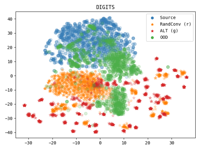
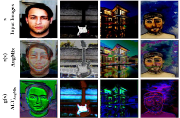
Figure 2: (Left) tSNE plot showing the discrepancy between the source distribution (MNIST) and the out-of-distribution datasets for the “Digits” benchmark. The diversity introduced by ALT is much larger and wide-spread than data augmentation techniques such as RandConv. (Right) Qualitative Comparison of PACS images transformed by RandConv data augmentation vs. ALT (ALT_RandConv), illustrating the wide range of transformations learned by ALT.

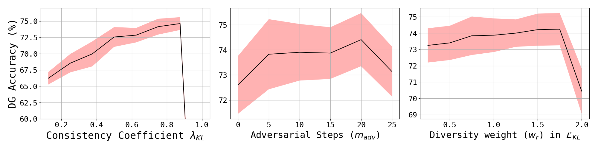
Figure 3: Analysis: We study the effect of each hyper-parameter in ALT on the average accuracy using the Digits benchmark (shown as 1 standard deviation around the mean over 5 runs). We observe that the consistency (left) is generally important until a certain point, after which it becomes harmful; (middle) taking more adversarial steps improves performance; (right) surprisingly, we find that the trade-off between diversity and adversity is non- trivial and dataset dependent. In our benchmarking experiments (Tables 1, 2 , 3) we do not perform any hyper-parameter tuning, and set $w_{r}{=}1$, i.e. equal weight to adversity and diversity.

5 Analysis of ALT

In this section we study the various components of ALT, and provide insights into their impact on generalization.

5.1 ALT is better than naïve diversity.

Our first big insight is that ALT without an explicit diversity (ALT_g-only) module still outperforms all the top performing methods across the benchmarks we evaluated on, indicating that learned adversarial transformations are a powerful way to train classifiers for generalization.

Our next observation is that ALT makes the choice of diversity module fairly arbitrary. We see this effect on multiple benchmarks – for example, on the Digits benchmark shown in Table 3, AugMix has a relatively poor generalization performance when compared with the baseline ERM whereas ALT_Augmix achieves state of the art. This is again seen in the Office-Home benchmark shown in Table 2, where RandConv is worse than ERM, but ALT_RandConv is the best performing method. Thus, irrespective of the choice of diversity module, the adversarially learned transformations benefit generalization on all benchmarks.

In Figure 2 (left panel) we analyze the diversity introduced by ALT on the Digits benchmark, in comparison to the source distribution the target (OOD) distribution and the distribution of RandConv augmentations. While RandConv does simulate a domain shift compared to the source, most RandConv points are clustered close to each other. However, the diversity due to ALT is considerably larger and ALT samples are spread widely across the tSNE space. We believe this is because data augmentation functions have a fixed types of diversity (random convolution filter in the case of RandConv), while ALT searches for adversarial transformations for each batch – this leads to novel types of diversity for each batch of training samples. We also show qualitative examples of the image transformations learned with ALT in Figure 2, and it is clear that ALT achieves far more diverse and larger transformations of the input images than previous data augmentation techniques. A similar comparison of ALT with AugMix [22] is shown in the supplementary material.

5.2 Effect of Varying ALT Hyperparameters.

The three main hyper-parameters that control ALT are: (1) $\lambda_{KL}$ – the coefficient in Eq. 5 which decides the weight for the KL-divergence consistency in the total loss, (2) $m_{adv}$ – the number of adversarial steps in the adversarial maximization of Eq. 4, and (3) $w_{r}$ – the diversity weight which controls the interaction between the diversity module $r()$ and the adversary network $g()$ in Eq. 6. We investigate the effect of each of these on domain generalization accuracy in Figure 3. The first plot shows that the consistency coefficient $\lambda_{KL}$ is impactful and a higher value leads to better generalization. However at $\lambda_{KL}=1.0$ the accuracy degenerates to random performance; this is expected as the classifier loss gets $1-\lambda_{KL}{=}0$ weight. From the second plot, we observe that the optimal number of adversarial steps is around 20. Note that performance at all non-zero values of $m_{adv}$ that we tried $(5,10,15,20,25)$ is greater than previous state-of-the-art. The importance of the adversarial module is evident from the third plot – performance at $w_{r}=0$ (adversarial module only) is higher than performance of $w_{r}=2$ (diversity module only), and the combination of both modules yields the best result. Clearly, the adversarial component is a critical factor that causes improvements in generalization.

6 Conclusion

In this paper, we address the problem of single source domain generalization. Our approach, Adversarially Learned Transformations (ALT) updates a convolutional network to learn plausible image transformations of the source domain that can fool the classifier during training; and enforces a consistency constraint on the predictions on clean images and transformed images. ALT is a significant improvement over prior methods that utilize pixel-wise perturbations. We showed that this strategy outperforms all existing techniques, including standard data augmentation methods, on multiple benchmarks because it is able to generate a diverse set of large transformations of the source domain. We also find that ALT can be naturally combined with existing diversity modules like RandConv or AugMix to improve their performance. We studied components of ALT through extensive ablations and analysis to obtain insights into its performance gains. Our studies indicate that naïve diversity alone is insufficient, but needs to be combined with adversarially learned transformations to maximize generalization performance.

Acknowledgements: This work was performed under the auspices of the U.S. Department of Energy by the Lawrence Livermore National Laboratory under Contract No. DE-AC52-07NA27344, Lawrence Livermore National Security, LLC. and was supported by the LDRD Program under project 22-ERD-006 with IM release number LLNL-JRNL-836221. BK’s efforts were supported by 22-DR-009. TG, CB, and YY were supported by NSF RI grants #1816039 and #2132724.

Appendix

This appendix contains training settings, additional results and visualizations to supplement the main paper. We also discuss the limitations of ALT and scope for future work in this direction. Code to reproduce experiments has been released publicly: https://github.com/tejas-gokhale/ALT.

Appendix A Training Settings

Table 4 shows the training settings and hyperparameters used for experiments on each benchmark. See Algorithm 1 in the main paper for context and relevant equations.

Appendix B Detailed Results

We provide detailed results including standard deviation values for our models on the PACS and Office-Home benchmarks, for each source domain. We compare these with RandConv [43], AugMix [22], and a combination of RandConv and AugMix which utilizes AugMix as one of the two augmentations in the consistency constraint of RandConv. Results of the PACS experiments are shown in Tables 6, 7, 8, 9, when using P, A, C, and S as the source datasets, respectively. Results of the Office-Home experiments are show in Tables 10, 11, 12, 13, when using R, A, C, and P as the source datasets, respectively.

Appendix C Visualizations

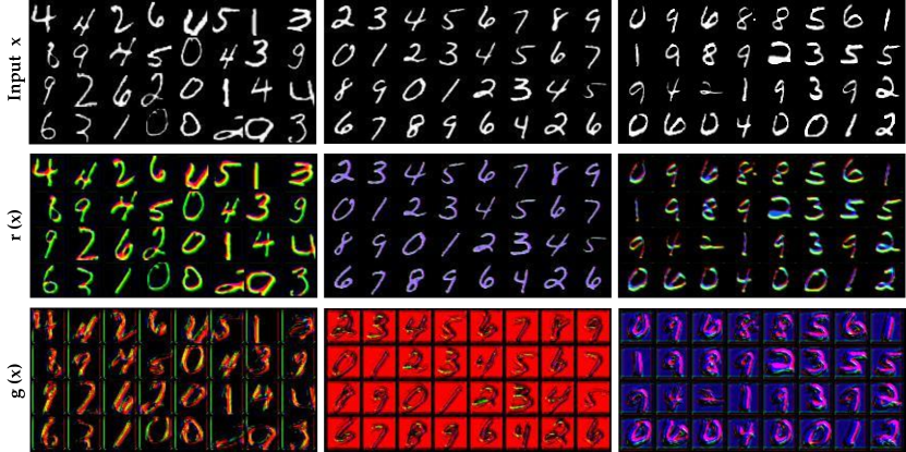
Figure 7: Digits: Comparison of images transformed by RandConv and ALT_RandConv with MNIST10k as source dataset.

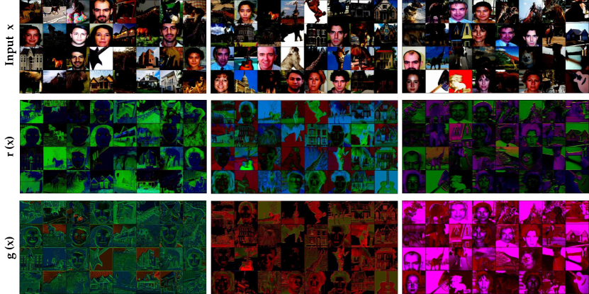
Figure 8: PACS: Comparison of images transformed by RandConv and ALT_RandConv with Photo as source dataset.

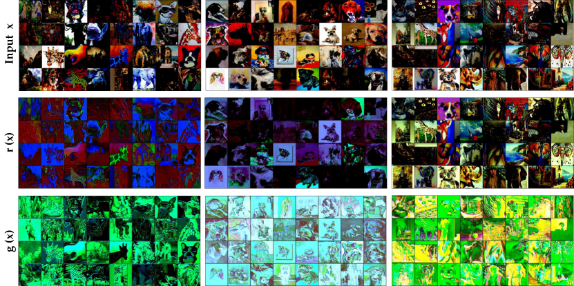
Figure 9: PACS: Comparison of images transformed by RandConv and ALT_RandConv with Art-Painting as source dataset.

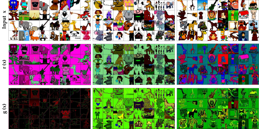
Figure 10: PACS: Comparison of images transformed by RandConv and ALT_RandConv with Cartoon as source dataset.

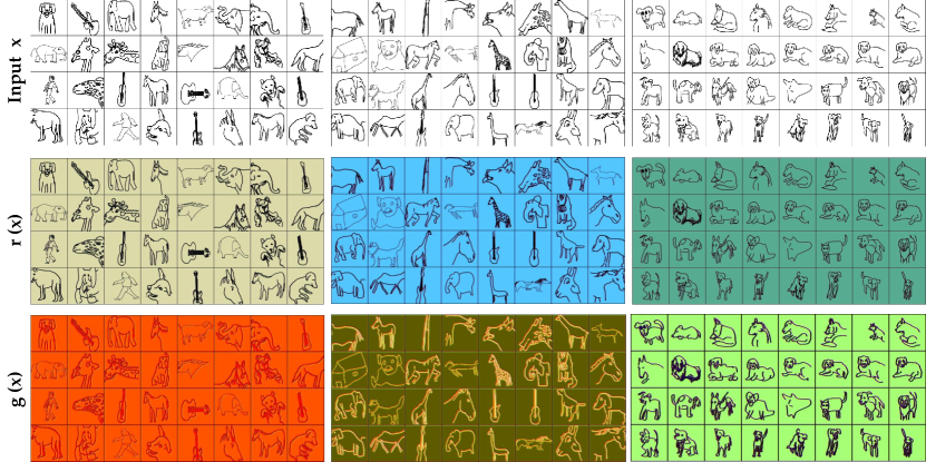
Figure 11: PACS: Comparison of images transformed by RandConv and ALT_RandConv with Sketch as source dataset.

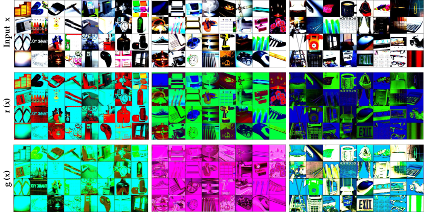
Figure 12: Office-Home: Comparison of images transformed by RandConv and ALT_RandConv with Real as source dataset.

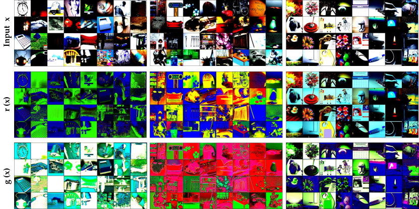
Figure 13: Office-Home: Comparison of images transformed by RandConv and ALT_RandConv with Art as source dataset.

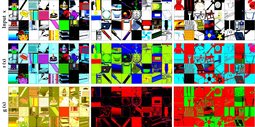
Figure 14: Office-Home: Comparison of images transformed by RandConv and ALT_RandConv with Clipart as source dataset.

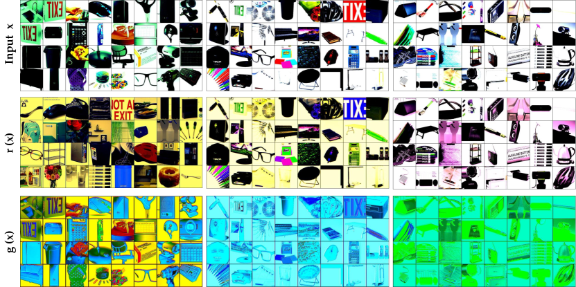
Figure 15: Office-Home: Comparison of images transformed by RandConv and ALT_RandConv with Product as source dataset.

In this section, we provide additional visualizations and qualitative examples for augmented images generated by ALT, for Digits (Figure 7), PACS (Figures 8, 9, 10, 11), and Office-Home PACS (Figures 12, 13, 14, 15). In each figure, the first row shows input images $\operatorname{\mathrm{x}}$, the second row shows the outputs of the diversity module $r(\operatorname{\mathrm{x}})$, and the third row shows the outputs of the adversary network $g(\operatorname{\mathrm{x}})$.

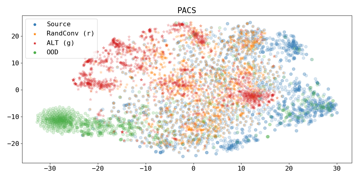
Figure 5: tSNE plot showing the discrepancy between the source distribution and the out-of-distribution datasets for the PACS benchmark.

In Figure 5 and 6 we show an illustration of the diversity introduced by ALT in comparison to the source distribution, the target (OOD) distribution, and the distribution of RandConv augmentations, for the PACS and OfficeHome benchmarks respectively. The diversity introduced by ALT is much larger and wide-spread than data augmentation techniques such as RandConv.

Variable	Digits	PACS	Office-Home
$f$ architecture	DigitNet [41]	ResNet18 [20]	ResNet50 [20]
$g$ architecture	{conv${}_{kernel=3,stride=1,padding=1,leakyReLU_{p=0.2}}\}\times 4$
$\rho_{0},\phi_{0}$	Kaiming Normal Initialization [19]
$T$	10000	2000	2000
$T_{pre}$	1250	400	400
$\eta$	1e-4	0.004	0.004
$m_{adv}$	10	10	10
$\eta_{adv}$	5e-6	5e-5	5e-5
$w_{r}$	1.0	1.0	1.0
$\lambda_{KL}$	0.75	0.75	0.75

Table 4: Training settings and hyper-parameters for experiments on each benchmark.

Appendix D Limitations and Future Directions

In this paper we have explored the effectiveness of ALT on three standard domain generalization benchmarks. For fair comparison, for each baseline model, we use the same model architecture and training settings as the backbone – for instance, ERM, RandConv, AugMix and ALT are all trained with the same hyperparameters as shown in Table 4. For significance of results, we have repeated each experiment (including those in analyses) for 5 different seeds and have reported mean and standard deviation.

D.1 Complexity of Adversary Network.

One limitation (and therefore scope for future work) is that we have considered one family of architecture for our adversary network $g$ – fully convolutional image-to-image translation networks. We conduct additional analysis to understand how this choice affects generalization performance, and compare performance when using between 2 and 6 convolutional layers. We reuse all other training settings from our benchmark model $ALT_{RandConv}$ on both Digits and PACS. Results are shown in Table 5.

For PACS and OfficHome, we observe that all ALT models compared are better than previous baselines including AugMix and RandConv. For Digits, we observe that performance of ALT with a 2-layer $g$ is close to RandConv, and is greater than all previous baselines for higher depth of the network. We do not see a clear correlation across datasets between the number of layers and the domain generalization performance. Investigating the dynamics of model capacity of the adversary network and how it may affect domain generalization, is an interesting direction for future work.

		FCN Number of Layers
Benchmark		2	3	4	5	6
Digits		72.75	73.74	74.10	73.87	74.15
PACS		63.40	63.92	64.41	64.20	63.78
OfficeHome		59.67	59.56	59.79	59.42	59.45

Table 5: Effect of the depth (number of convolutional layers) of the adversity network $g$ on average domain generalization on all three benchmarks.

It may be possible that more complex generative architectures (i.e. greater complexity of transformations) may be needed for larger domain shift is larger, to model diversity and adversity for a given source domain. Thus the choice of architecture for $g$ is an interesting direction; nevertheless, in this paper we show that the simple fully convolutional architecture gives us performance boosts in all three datasets.

We believe that ideas presented in this paper, although evaluated on image classification, have the potential of being widely applicable to many other vision tasks for domain generalization. They may also be applied to other application areas such as audio or text, where the transformation function $g$ may take different forms.

Method	Photo⋆	Art-Painting	Cartoon	Sketch	Target Avg.	PACS Avg.
RandConv	96.407 $\pm$0.757	61.309 $\pm$2.316	37.577 $\pm$2.257	50.463 $\pm$9.018	49.783 $\pm$4.255	61.439 $\pm$3.217
AugMix	99.532 $\pm$0.438	68.633 $\pm$0.950	33.788 $\pm$1.205	36.304 $\pm$2.801	46.242 $\pm$1.122	59.564 $\pm$0.930
RandConv + AugMix	98.363 $\pm$0.438	65.527 $\pm$3.060	39.300 $\pm$6.237	40.901 $\pm$5.073	48.576 $\pm$4.031	61.023 $\pm$3.001
ALTg-only	99.064 $\pm$ 0.286	68.770 $\pm$ 0.932	43.387 $\pm$ 1.142	50.832 $\pm$ 2.937	54.330 $\pm$ 1.078	65.513 $\pm$ 0.757
ALTRandConv	98.947 $\pm$0.234	68.740 $\pm$0.702	40.828 $\pm$2.537	56.024 $\pm$2.009	55.197 $\pm$0.498	66.135 $\pm$0.330
ALTAugMix	99.298 $\pm$0.438	68.506 $\pm$0.836	43.507 $\pm$2.615	53.271 $\pm$4.149	55.094 $\pm$1.876	66.145 $\pm$1.387

Table 6: SSDG performance on PACS for the P$\rightarrow$ACS setting. ^⋆Source Domain. bold: best result.

Method	Photo	Art Painting⋆	Cartoon	Sketch	Target Avg.	PACS Avg.
RandConv	87.281 $\pm$0.796	85.437 $\pm$0.532	61.143 $\pm$2.752	60.519 $\pm$4.050	69.648 $\pm$2.152	73.595 $\pm$1.582
AugMix	95.317 $\pm$0.422	93.077 $\pm$1.276	64.061 $\pm$0.361	55.027 $\pm$2.195	71.469 $\pm$0.637	76.871 $\pm$0.581
RandConv + AugMix	90.743 $\pm$0.781	90.481 $\pm$0.638	64.206 $\pm$2.238	62.515 $\pm$2.854	72.488 $\pm$1.731	76.986 $\pm$1.177
ALTg-only	94.934 $\pm$0.269	91.058 $\pm$0.720	63.524 $\pm$1.821	63.813 $\pm$2.249	74.090 $\pm$1.086	78.332 $\pm$0.845
ALTRandConv	93.593 $\pm$0.328	92.596 $\pm$1.036	64.044 $\pm$0.635	65.991 $\pm$1.130	74.543 $\pm$0.537	79.056 $\pm$0.609
ALTAugMix	93.174 $\pm$0.437	91.442 $\pm$0.638	65.683 $\pm$1.656	68.226 $\pm$2.453	75.694 $\pm$1.214	79.631 $\pm$0.856

Table 7: SSDG performance on PACS for the A$\rightarrow$PCS setting. ^⋆Source Domain. bold: best result.

Method	Photo	Art-Painting	Cartoon⋆	Sketch	Target Avg.	PACS Avg.
RandConv	73.677 $\pm$1.814	57.051 $\pm$1.764	91.66 $\pm$0.876	72.855 $\pm$2.314	67.861 $\pm$1.550	73.810 $\pm$1.317
AugMix	84.599 $\pm$0.997	68.281 $\pm$2.085	96.287 $\pm$0.940	71.097 $\pm$0.609	74.659 $\pm$1.088	80.066 $\pm$0.897
RandConv + AugMix	78.790 $\pm$0.975	65.400 $\pm$1.611	93.840 $\pm$1.020	71.285 $\pm$2.730	71.825 $\pm$1.315	77.329 $\pm$1.105
ALTg-only	84.575 $\pm$1.047	68.867 $\pm$2.126	94.768 $\pm$0.43	74.421 $\pm$0.441	75.954 $\pm$1.119	80.658 $\pm$0.929
ALTRandConv	83.916 $\pm$0.51	68.086 $\pm$1.901	95.190 $\pm$0.686	74.487 $\pm$0.505	75.496 $\pm$0.799	80.420 $\pm$0.644
ALTAugMix	85.964 $\pm$1.098	71.943 $\pm$1.234	94.599 $\pm$0.560	74.172 $\pm$0.752	77.360 $\pm$0.734	81.670 $\pm$0.667

Table 8: SSDG performance on PACS for the C$\rightarrow$PAS setting. ^⋆Source Domain. bold: best result.

Method	Photo	Art-Painting	Cartoon	Sketch⋆	Target Avg.	PACS Avg.
RandConv	46.132 $\pm$4.879	52.168 $\pm$1.623	63.942 $\pm$2.219	94.264 $\pm$0.673	54.081 $\pm$1.959	64.126 $\pm$1.465
AugMix	46.731 $\pm$2.916	37.852 $\pm$1.878	58.575 $\pm$1.747	94.221 $\pm$0.711	47.719 $\pm$1.723	59.345 $\pm$1.268
RandConv + AugMix	54.359 $\pm$0.819	46.074 $\pm$2.709	61.246 $\pm$1.245	94.171 $\pm$0.582	53.893 $\pm$0.945	63.963 $\pm$0.787
ALTg-only	49.305 $\pm$2.775	39.658 $\pm$3.423	61.109 $\pm$1.853	94.573 $\pm$0.466	50.024 $\pm$2.408	61.161 $\pm$1.726
ALTRandConv	51.305 $\pm$0.866	41.787 $\pm$1.174	62.773 $\pm$1.089	94.724 $\pm$0.527	51.955 $\pm$0.791	62.647 $\pm$0.571
ALTAugMix	49.078 $\pm$2.072	40.186 $\pm$2.494	62.901 $\pm$0.358	94.271 $\pm$0.624	50.721 $\pm$1.414	61.609 $\pm$1.103

Table 9: SSDG performance on PACS for the S$\rightarrow$PAC setting. ^⋆Source Domain. bold: best result.

Method	Real⋆	Art	Clipart	Product	Target Avg.	Office-Home Avg.
RandConv	83.028 $\pm$2.067	59.021 $\pm$0.916	47.269 $\pm$1.251	72.172 $\pm$0.418	59.487 $\pm$0.792	65.372 $\pm$1.096
AugMix	87.294 $\pm$1.21	64.101 $\pm$0.882	47.564 $\pm$0.158	75.956 $\pm$0.32	62.54 $\pm$0.345	68.729 $\pm$0.490
RandConv + AugMix	81.514 $\pm$0.515	59.167 $\pm$0.722	48.180 $\pm$1.024	71.166 $\pm$0.445	59.504 $\pm$0.256	65.007 $\pm$0.226
ALTg-only	86.514 $\pm$0.622	64.622 $\pm$0.490	53.327 $\pm$0.344	76.276 $\pm$0.117	64.742 $\pm$0.122	70.185 $\pm$0.138
ALTRandConv	87.477 $\pm$1.042	64.879 $\pm$0.439	53.097 $\pm$0.554	76.066 $\pm$0.447	64.681 $\pm$0.290	70.380 $\pm$0.312
ALTAugMix	86.560 $\pm$0.980	64.860 $\pm$0.267	53.271 $\pm$0.799	76.286 $\pm$0.347	64.806 $\pm$0.327	70.244 $\pm$0.461

Table 10: SSDG performance on Office-Home for the R$\rightarrow$ACP setting. ^⋆Source Domain. bold: best result.

Method	Real	Art⋆	Clipart	Product	Target Avg.	Office-Home Avg.
RandConv	66.915 $\pm$1.069	72.428 $\pm$2.066	42.387 $\pm$1.405	55.045 $\pm$1.547	54.782 $\pm$1.297	59.194 $\pm$1.427
AugMix	71.887 $\pm$0.432	80.494 $\pm$1.342	45.314 $\pm$0.768	61.882 $\pm$0.382	59.694 $\pm$0.427	64.894 $\pm$0.369
RandConv + AugMix	65.620 $\pm$0.632	71.852 $\pm$1.758	42.606 $\pm$1.026	54.434 $\pm$0.774	54.220 $\pm$0.617	58.628 $\pm$0.862
ALTg-only	71.193 $\pm$0.308	78.930 $\pm$1.146	47.340 $\pm$0.331	61.151 $\pm$0.561	59.895 $\pm$0.283	64.654 $\pm$0.259
ALTRandConv	71.754 $\pm$0.286	78.025 $\pm$1.181	48.328 $\pm$0.787	61.186 $\pm$0.429	60.423 $\pm$0.280	64.823 $\pm$0.474
ALTAugMix	71.122 $\pm$0.540	79.095 $\pm$1.634	48.058 $\pm$0.632	61.156 $\pm$0.813	60.112 $\pm$0.590	64.858 $\pm$0.518

Table 11: SSDG performance on Office-Home for the A$\rightarrow$RCP setting. ^⋆Source Domain. bold: best result.

Method	Real	Art	Clipart⋆	Product	Target Avg.	Office-Home Avg.
RandConv	58.944 $\pm$0.521	44.741 $\pm$0.714	80.320 $\pm$1.073	56.211 $\pm$1.141	53.299 $\pm$0.711	60.054 $\pm$0.771
AugMix	62.244 $\pm$0.526	49.309 $\pm$0.879	81.510 $\pm$0.885	58.939 $\pm$0.584	56.831 $\pm$0.530	63.000 $\pm$0.454
RandConv + AugMix	57.914 $\pm$0.730	43.698 $\pm$0.511	77.986 $\pm$1.087	55.040 $\pm$0.683	52.217 $\pm$0.249	58.660 $\pm$0.417
ALTg-only	61.968 $\pm$0.849	49.977 $\pm$0.987	80.320 $\pm$1.073	58.779 $\pm$0.743	56.908 $\pm$0.808	62.761 $\pm$0.733
ALTRandConv	62.264 $\pm$0.560	50.133 $\pm$0.956	80.732 $\pm$0.637	58.819 $\pm$0.558	57.072 $\pm$0.539	62.987 $\pm$0.455
ALTAugMix	61.841 $\pm$0.382	50.426 $\pm$1.070	80.824 $\pm$0.510	58.839 $\pm$0.559	57.035 $\pm$0.580	62.982 $\pm$0.526

Table 12: SSDG performance on Office-Home for the C$\rightarrow$RAP setting. ^⋆Source Domain. bold: best result.

Method	Real	Art	Clipart	Product⋆	Target Avg.	Office-Home Avg.
RandConv	66.318 $\pm$0.240	43.524 $\pm$0.664	43.365 $\pm$1.058	90.135 $\pm$0.643	51.069 $\pm$0.607	60.836 $\pm$0.372
AugMix	71.515 $\pm$0.706	50.041 $\pm$0.688	42.596 $\pm$0.619	91.622 $\pm$0.263	54.717 $\pm$0.518	63.943 $\pm$0.453
RandConv + AugMix	65.523 $\pm$0.753	43.240 $\pm$1.454	41.710 $\pm$0.621	89.459 $\pm$0.785	50.158 $\pm$0.900	59.983 $\pm$0.865
ALTg-only	70.082 $\pm$0.532	48.842 $\pm$0.648	46.877 $\pm$0.552	91.306 $\pm$0.544	55.267 $\pm$0.302	64.277 $\pm$0.171
ALTRandConv	70.530 $\pm$0.359	49.208 $\pm$0.418	47.025 $\pm$0.498	91.577 $\pm$0.506	55.588 $\pm$0.300	64.585 $\pm$0.212
ALTAugMix	70.637 $\pm$0.301	49.318 $\pm$1.008	47.554 $\pm$0.458	91.396 $\pm$0.798	55.837 $\pm$0.383	64.726 $\pm$0.361

Table 13: SSDG performance on Office-Home for the P$\rightarrow$RAC setting. ^⋆Source Domain. bold: best result.

Figure 4: tSNE plot showing the discrepancy between the source distribution and the out-of-distribution datasets for the Digits benchmark.

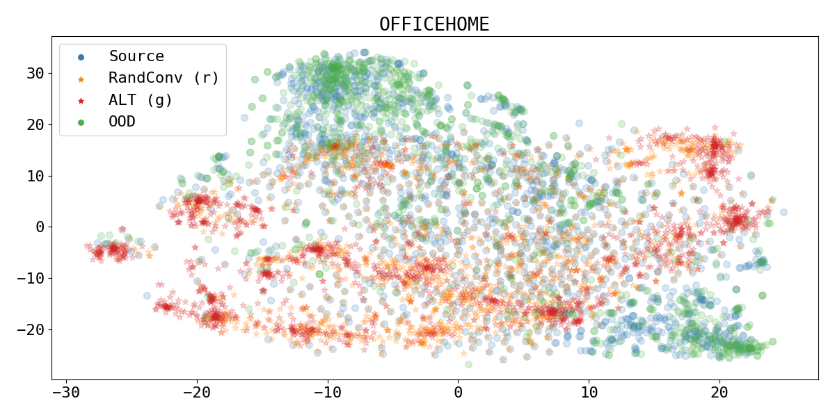
Figure 6: tSNE plot showing the discrepancy between the source distribution and the out-of-distribution datasets for the OfficeHome benchmark.

References

- [1] Martin Arjovsky, Léon Bottou, Ishaan Gulrajani, and David Lopez-Paz. Invariant risk minimization. arXiv preprint arXiv:1907.02893, 2019.
- [2] Gregory W Benton, Marc Finzi, Pavel Izmailov, and Andrew Gordon Wilson. Learning invariances in neural networks from training data. In NeurIPS, 2020.
- [3] Nicholas Carlini and David Wagner. Towards evaluating the robustness of neural networks. In 2017 ieee symposium on security and privacy (sp), pages 39–57. IEEE, 2017.
- [4] Fabio M Carlucci, Antonio D’Innocente, Silvia Bucci, Barbara Caputo, and Tatiana Tommasi. Domain generalization by solving jigsaw puzzles. In Proceedings of the IEEE/CVF Conference on Computer Vision and Pattern Recognition, pages 2229–2238, 2019.
- [5] Gabriela Csurka. Domain adaptation for visual applications: A comprehensive survey. arXiv preprint arXiv:1702.05374, 2017.
- [6] Ekin D Cubuk, Barret Zoph, Dandelion Mane, Vijay Vasudevan, and Quoc V Le. Autoaugment: Learning augmentation strategies from data. In Proceedings of the IEEE/CVF Conference on Computer Vision and Pattern Recognition, pages 113–123, 2019.
- [7] Ekin D Cubuk, Barret Zoph, Jonathon Shlens, and Quoc V Le. Randaugment: Practical automated data augmentation with a reduced search space. In Proceedings of the IEEE/CVF Conference on Computer Vision and Pattern Recognition Workshops, pages 702–703, 2020.
- [8] Jia Deng, Wei Dong, Richard Socher, Li-Jia Li, Kai Li, and Fei-Fei Li. Imagenet: A large-scale hierarchical image database. In 2009 IEEE Computer Society Conference on Computer Vision and Pattern Recognition (CVPR 2009), 20-25 June 2009, Miami, Florida, USA, pages 248–255. IEEE Computer Society, 2009.
- [9] JS Denker, WR Gardner, HP Graf, D Henderson, RE Howard, W Hubbard, LD Jackel, HS Baird, and I Guyon. Neural network recognizer for hand-written zip code digits. In Proceedings of the 1st International Conference on Neural Information Processing Systems, pages 323–331, 1988.
- [10] Terrance DeVries and Graham W Taylor. Improved regularization of convolutional neural networks with cutout. arXiv preprint arXiv:1708.04552, 2017.
- [11] Guneet S Dhillon, Kamyar Azizzadenesheli, Zachary C Lipton, Jeremy D Bernstein, Jean Kossaifi, Aran Khanna, and Animashree Anandkumar. Stochastic activation pruning for robust adversarial defense. In International Conference on Learning Representations, 2018.
- [12] Yinpeng Dong, Fangzhou Liao, Tianyu Pang, Hang Su, Jun Zhu, Xiaolin Hu, and Jianguo Li. Boosting adversarial attacks with momentum. In Proceedings of the IEEE conference on computer vision and pattern recognition, pages 9185–9193, 2018.
- [13] Yaroslav Ganin and Victor Lempitsky. Unsupervised domain adaptation by backpropagation. In International conference on machine learning, pages 1180–1189. PMLR, 2015.
- [14] Yaroslav Ganin, Evgeniya Ustinova, Hana Ajakan, Pascal Germain, Hugo Larochelle, François Laviolette, Mario Marchand, and Victor Lempitsky. Domain-adversarial training of neural networks. The journal of machine learning research, 17(1):2096–2030, 2016.
- [15] Robert Geirhos, Carlos R Medina Temme, Jonas Rauber, Heiko H Schütt, Matthias Bethge, and Felix A Wichmann. Generalisation in humans and deep neural networks. In Proceedings of the 32nd International Conference on Neural Information Processing Systems, pages 7549–7561, 2018.
- [16] Tejas Gokhale, Rushil Anirudh, Bhavya Kailkhura, Jayaraman J Thiagarajan, Chitta Baral, and Yezhou Yang. Attribute-guided adversarial training for robustness to natural perturbations. In Proceedings of the AAAI Conference on Artificial Intelligence, volume 35, pages 7574–7582, 2021.
- [17] Ian J. Goodfellow, Jonathon Shlens, and Christian Szegedy. Explaining and harnessing adversarial examples. In Yoshua Bengio and Yann LeCun, editors, 3rd International Conference on Learning Representations, ICLR 2015, San Diego, CA, USA, May 7-9, 2015, Conference Track Proceedings, 2015.
- [18] Ishaan Gulrajani and David Lopez-Paz. In search of lost domain generalization. In ICML, 2021.
- [19] Kaiming He, Xiangyu Zhang, Shaoqing Ren, and Jian Sun. Delving deep into rectifiers: Surpassing human-level performance on imagenet classification. In Proceedings of the IEEE international conference on computer vision, pages 1026–1034, 2015.
- [20] Kaiming He, Xiangyu Zhang, Shaoqing Ren, and Jian Sun. Deep residual learning for image recognition. In 2016 IEEE Conference on Computer Vision and Pattern Recognition, CVPR 2016, Las Vegas, NV, USA, June 27-30, 2016, pages 770–778. IEEE Computer Society, 2016.
- [21] Dan Hendrycks and Thomas G. Dietterich. Benchmarking neural network robustness to common corruptions and perturbations. In 7th International Conference on Learning Representations, ICLR 2019, New Orleans, LA, USA, May 6-9, 2019. OpenReview.net, 2019.
- [22] Dan Hendrycks, Norman Mu, Ekin Dogus Cubuk, Barret Zoph, Justin Gilmer, and Balaji Lakshminarayanan. Augmix: A simple data processing method to improve robustness and uncertainty. In 8th International Conference on Learning Representations, ICLR 2020, Addis Ababa, Ethiopia, April 26-30, 2020. OpenReview.net, 2020.
- [23] Yunseok Jang, Tianchen Zhao, Seunghoon Hong, and Honglak Lee. Adversarial defense via learning to generate diverse attacks. In Proceedings of the IEEE/CVF International Conference on Computer Vision, pages 2740–2749, 2019.
- [24] Pang Wei Koh, Shiori Sagawa, Sang Michael Xie, Marvin Zhang, Akshay Balsubramani, Weihua Hu, Michihiro Yasunaga, Richard Lanas Phillips, Irena Gao, Tony Lee, et al. Wilds: A benchmark of in-the-wild distribution shifts. In International Conference on Machine Learning, pages 5637–5664. PMLR, 2021.
- [25] S Kullback, RA Leibler, et al. On information and sufficiency. Annals of Mathematical Statistics, 22(1):79–86, 1951.
- [26] Yann LeCun, Léon Bottou, Yoshua Bengio, and Patrick Haffner. Gradient-based learning applied to document recognition. Proceedings of the IEEE, 86(11):2278–2324, 1998.
- [27] Da Li, Yongxin Yang, Yi-Zhe Song, and Timothy M Hospedales. Deeper, broader and artier domain generalization. In Proceedings of the IEEE international conference on computer vision, pages 5542–5550, 2017.
- [28] Da Li, Yongxin Yang, Yi-Zhe Song, and Timothy M Hospedales. Learning to generalize: Meta-learning for domain generalization. In Thirty-Second AAAI Conference on Artificial Intelligence, 2018.
- [29] Seyed-Mohsen Moosavi-Dezfooli, Alhussein Fawzi, and Pascal Frossard. Deepfool: a simple and accurate method to fool deep neural networks. In Proceedings of the IEEE conference on computer vision and pattern recognition, pages 2574–2582, 2016.
- [30] Norman Mu and Justin Gilmer. Mnist-c: A robustness benchmark for computer vision. arXiv preprint arXiv:1906.02337, 2019.
- [31] Hyeonseob Nam, HyunJae Lee, Jongchan Park, Wonjun Yoon, and Donggeun Yoo. Reducing domain gap by reducing style bias. In Proceedings of the IEEE/CVF Conference on Computer Vision and Pattern Recognition, pages 8690–8699, 2021.
- [32] Yuval Netzer, Tao Wang, Adam Coates, Alessandro Bissacco, Bo Wu, and Andrew Y Ng. Reading digits in natural images with unsupervised feature learning. 2011.
- [33] Fengchun Qiao, Long Zhao, and Xi Peng. Learning to learn single domain generalization. In 2020 IEEE/CVF Conference on Computer Vision and Pattern Recognition, CVPR 2020, Seattle, WA, USA, June 13-19, 2020, pages 12553–12562. IEEE, 2020.
- [34] Alexander J Ratner, Henry R Ehrenberg, Zeshan Hussain, Jared Dunnmon, and Christopher Ré. Learning to compose domain-specific transformations for data augmentation. Advances in neural information processing systems, 30:3239, 2017.
- [35] Alexander Robey, George J Pappas, and Hamed Hassani. Model-based domain generalization. arXiv preprint arXiv:2102.11436, 2021.
- [36] Leonid I Rudin, Stanley Osher, and Emad Fatemi. Nonlinear total variation based noise removal algorithms. Physica D: nonlinear phenomena, 60(1-4):259–268, 1992.
- [37] William B Shen, Danfei Xu, Yuke Zhu, Leonidas J Guibas, Li Fei-Fei, and Silvio Savarese. Situational fusion of visual representation for visual navigation. In Proceedings of the IEEE/CVF International Conference on Computer Vision, pages 2881–2890, 2019.
- [38] Igor Vasiljevic, Ayan Chakrabarti, and Gregory Shakhnarovich. Examining the impact of blur on recognition by convolutional networks. arXiv preprint arXiv:1611.05760, 2016.
- [39] Hemanth Venkateswara, Jose Eusebio, Shayok Chakraborty, and Sethuraman Panchanathan. Deep hashing network for unsupervised domain adaptation. In Proceedings of the IEEE Conference on Computer Vision and Pattern Recognition, pages 5018–5027, 2017.
- [40] Riccardo Volpi and Vittorio Murino. Addressing model vulnerability to distributional shifts over image transformation sets. In Proceedings of the IEEE/CVF International Conference on Computer Vision, pages 7980–7989, 2019.
- [41] Riccardo Volpi, Hongseok Namkoong, Ozan Sener, John C. Duchi, Vittorio Murino, and Silvio Savarese. Generalizing to unseen domains via adversarial data augmentation. In Advances in Neural Information Processing Systems, pages 5339–5349, 2018.
- [42] Eric Wong and J Zico Kolter. Learning perturbation sets for robust machine learning. In International Conference on Learning Representations, 2020.
- [43] Zhenlin Xu, Deyi Liu, Junlin Yang, Colin Raffel, and Marc Niethammer. Robust and generalizable visual representation learning via random convolutions. In International Conference on Learning Representations, 2020.
- [44] Xiaoyong Yuan, Pan He, Qile Zhu, and Xiaolin Li. Adversarial examples: Attacks and defenses for deep learning. IEEE transactions on neural networks and learning systems, 30(9):2805–2824, 2019.
- [45] Sangdoo Yun, Dongyoon Han, Seong Joon Oh, Sanghyuk Chun, Junsuk Choe, and Youngjoon Yoo. Cutmix: Regularization strategy to train strong classifiers with localizable features. In Proceedings of the IEEE/CVF International Conference on Computer Vision, pages 6023–6032, 2019.
- [46] Hongyi Zhang, Moustapha Cisse, Yann N Dauphin, and David Lopez-Paz. mixup: Beyond empirical risk minimization. In International Conference on Learning Representations, 2018.
- [47] Xinyu Zhang, Qiang Wang, Jian Zhang, and Zhao Zhong. Adversarial autoaugment. In International Conference on Learning Representations, 2019.
- [48] Zhun Zhong, Liang Zheng, Guoliang Kang, Shaozi Li, and Yi Yang. Random erasing data augmentation. In Proceedings of the AAAI Conference on Artificial Intelligence, volume 34, pages 13001–13008, 2020.
- [49] Kaiyang Zhou, Yongxin Yang, Timothy Hospedales, and Tao Xiang. Learning to generate novel domains for domain generalization. In European Conference on Computer Vision, pages 561–578. Springer, 2020.
- [50] Barret Zoph, Ekin D Cubuk, Golnaz Ghiasi, Tsung-Yi Lin, Jonathon Shlens, and Quoc V Le. Learning data augmentation strategies for object detection. In European Conference on Computer Vision, pages 566–583. Springer, 2020.