Magnetic Bloch Theorem and Reentrant Flat Bands in Twisted Bilayer Graphene at $2\pi$ Flux

Abstract

Bloch’s theorem is the centerpiece of topological band theory, which itself has defined an era of quantum materials research. However, Bloch’s theorem is broken by a perpendicular magnetic field, making it difficult to study topological systems in strong flux. For the first time, moiré materials have made this problem experimentally relevant, and its solution is the focus of this work. We construct gauge-invariant irreps of the magnetic translation group at $2\pi$ flux on infinite boundary conditions, allowing us to give analytical expressions in terms of the Siegel theta function for the magnetic Bloch Hamiltonian, non-Abelian Wilson loop, and many-body form factors. We illustrate our formalism using a simple square lattice model and the Bistritzer-MacDonald Hamiltonian of twisted bilayer graphene, obtaining reentrant ground states at $2\pi$ flux under the Coulomb interaction.

I Introduction

Motivated by developments in the fabrication of moiré materials with greatly enlarged unit cells Andrei et al. (2021); Cao et al. (2018, 2018); Kim et al. (2017); Balents et al. (2020); Liu and Dai (2021); Chu et al. (2020); Zang et al. (2021), this work revisits the solution of continuum Hamiltonians in strong flux from the modern perspective of topological band theory. The essential difficulty of the problem was identified by Zak who demonstrated that translations do not commute in generic magnetic flux and instead form a projective representation of the translation group Zak (1964a). As such, Bloch’s theorem does not apply. The result is a fractal energy spectrum as a function of magnetic flux known as the Hofstadter butterfly Hofstadter (1976, 1976); Albrecht et al. (2001); Hunt et al. (2013); Dean et al. (2013). In this work, we present a new formalism to obtain the exact band structure and topology of a continuum Hamiltonian when the flux through a single unit cell is $2\pi$. At $2\pi$ flux, corresponding to $\sim 25$T in magic angle twisted bilayer graphene (TBG) Bistritzer and MacDonald (2011a), the magnetic translation group commutes due to the Aharonov-Bohm effect, allowing reentrant Hofstadter phases Zak (1964a); Hofstadter (1976). Although methods already exist to study the spectrum in arbitrary magnetic fields Zak (1964b); Brown (1969); Streda (1982); Wannier (1978); Pereira et al. (2007); Xiao et al. (2010); Gumbs et al. (1995); Bistritzer and MacDonald (2011b); Töke et al. (2005); Greiter (2011); Bistritzer and MacDonald (2011); zhong Li et al. (1997); Crosse et al. (2020); Lian et al. (2021a); Pfannkuche and Gerhardts (1992); Arora et al. (2022), they are unsuitable for determining the topology and dominant many-body effects essential to moiré physics. Our formalism is manifestly gauge-invariant, leading to analytical expressions for the magnetic Bloch Hamiltonian, non-Abelian Berry connection, and many-body form factors. Importantly, numerical implementation is also straightforward, and we are able to study reentrant phases, which have recently become of interest Chaudhary et al. (2021); Cao et al. (2021), without using simplified models. The methods detailed here were used to study reentrant correlated insulators Herzog-Arbeitman et al. (2022) in twisted bilayer graphene, which have been observed in experiment Das et al. (2022).

We begin with a general discussion of the symmetry operators in Sec. II which are used to construct gauge-invariant magnetic translation group irreps on infinite boundary conditions in Sec. III. A discussion of the Siegel theta function DLMF, Siegel Theta ; Gunning (2012); Maloney and Witten (2020), a multi-dimensional generalization of the Jacobi theta function which appears in our states, may be found in App. A. We provide a general expression for the magnetic Bloch Hamiltonian in Sec. IV and compute the band structure for a square lattice model. Then in Sec. V, we define the Berry connection which receives two new magnetic contributions (Abelian and non-Abelian), and we discuss the topological transition between the strong flux or Landau level regime where the kinetic energy dominates and the crystalline regime where the potential dominates. In Sec. VII, we give convenient expressions for the form factors of generic density-density interactions. Finally in Secs. VIII and IX, we study the Bistritzer-MacDonald (BM) Hamiltonian Bistritzer and MacDonald (2011a) of twisted bilayer graphene which reaches $2\pi$ flux at $\sim 25$T. We discuss the symmetries of TBG at $2\pi$ and find that the degree of particle-hole breaking strongly determines the topology of the flat bands, which realize a decomposable elementary band representation Cano et al. (2018a).

We note that the Hofstadter spectrum of tight-binding models under the Peierls substitution Peierls (1933) is periodic in flux with the period equal to an integer multiple of $2\pi$ depending on the orbitals Herzog-Arbeitman et al. (2020). This is because gauge fields on the lattice are compact. Such systems differ from the continuum models considered here where there is no exact periodicity in $\phi$ (though see Ref. Kim et al. (2022) for a discussion of approximate periodicity) and we are not reliant on the validity of the Peierls approximation. Notably, the spectrum and topology of the BM model we obtain at $2\pi$ flux compares well to tight-binding calculations of twisted bilayer graphene at a small commensurate angle Guan et al. (2022).

II Symmetry Algebra

We consider a two-dimensional Hamiltonian minimally coupled to a background gauge field $\mathbf{A}(\mathbf{r})$ in the form

$$H =h(-i\boldsymbol{\nabla}-e\mathbf{A})+U(\mathbf{r}),\qquad\boldsymbol{\nabla}\times\mathbf{A}=B>0$$ (1)

where we study $h(p)=p^{2}/2m$ and $h(p)=v_{F}(p_{x}\sigma_{x}+p_{y}\sigma_{y})$ and set $\hbar=1$. Here $e>0$ is the electron charge, the magnetic field $B$ is perpendicular to the plane, and the cross product is a scalar in two dimensions. We neglect the Zeeman coupling, but it is trivial to add. The potential $U(\mathbf{r})$ is periodic: $U(\mathbf{r})=U(\mathbf{r}+\mathbf{R})$ where $\mathbf{R}$ is on the Bravais lattice with basis vectors $\mathbf{a}_{1},\mathbf{a}_{2}$ oriented so $\mathbf{a}_{1}\times\mathbf{a}_{2}=\Omega>0$. The reciprocal lattice is spanned by the vectors $2\pi\mathbf{b}_{i}$ satisfying $\mathbf{a}_{i}\cdot\mathbf{b}_{j}=\delta_{ij}$. The magnetic flux is $\phi=eB\Omega$ which is dimensionless (setting $\hbar=1$).

In absence of a periodic potential, the Hamiltonian $h(p)$ in flux can be solved in terms of Landau levels by introducing an oscillator algebra. The algebra is formed from the canonical momentum $\boldsymbol{\pi}=-i\boldsymbol{\nabla}-e\mathbf{A}$ obeying

$$\hbox{}[\pi_{\mu},\pi_{\nu}]=ie(\partial_{\mu}A_{\nu}-\partial_{\nu}A_{\mu})=ieB\epsilon_{\mu\nu}$$ (2)

where throughout this section, greek letters correspond to cartesian indices, e.g. $\mu,\nu\in\{x,y\}$, and we sum over repeated indices. We define the ladder operators $[a,a^{\dagger}]=1$ by

$$a =\frac{\pi_{x}+i\pi_{y}}{\sqrt{2eB}},a^{\dagger}=\frac{\pi_{x}-i\pi_{y}}{\sqrt{2eB}}\ .$$ (3)

In the simplest case of $h(p)=p^{2}/2m=eB(a^{\dagger}a+1/2)$ in magnetic field, the eigenstates are Landau levels given by powers of $a^{\dagger}$. The macroscopic degeneracy of the Landau levels is accounted for by the guiding center momenta $Q_{\mu}$. The gauge-invariant definition is

$$Q_{\mu} =\pi_{\mu}-eB\epsilon_{\mu\nu}x_{\nu}=-i\partial_{\mu}-e(A_{\mu}+B\epsilon_{\mu\nu}x_{\nu})\ .$$ (4)

The guiding center operators commute with the canonical momenta and obey

$$\hbox{}[Q_{\mu},\pi_{\nu}] =[\pi_{\mu}-eB\epsilon_{\mu\rho}x_{\rho},\pi_{\nu}]=ieB\epsilon_{\mu\nu}-ieB\epsilon_{\mu\nu}=0$$ (5)

$$[Q_{\mu},Q_{\nu}] =[\pi_{\mu}-eB\epsilon_{\mu\rho}x_{\rho},\pi_{\nu}-eB\epsilon_{\nu\sigma}x_{\sigma}]=-ieB\epsilon_{\mu\nu}\ .$$

The guiding centers form a separate oscillator system with $[b,b^{\dagger}]=1$ defined by (see App. A.1)

$$b =\frac{(\mathbf{a}_{1}-i\mathbf{a}_{2})\cdot\mathbf{Q}}{\sqrt{2\phi}},\quad b^{\dagger}=\frac{(\mathbf{a}_{1}+i\mathbf{a}_{2})\cdot\mathbf{Q}}{\sqrt{2\phi}},$$ (6)

Note that the $b$-oscillators commute with the $a$-oscillators by Eq. (81). Comparing Eq. (82) and Eq. (78), we see that the $a,a^{\dagger}$ operators are defined using cartesian variables while the $b,b^{\dagger}$ operators are defined using the lattice vectors. This is because the $a,a^{\dagger}$ operators are used to build the continuum kinetic term which has $SO(2)$ rotation symmetry, while the $b,b^{\dagger}$ operators will be used to construct states that respect the lattice periodicity.

The kinetic term $h(\boldsymbol{\pi})$, which is built out of $a$ and $a^{\dagger}$ operators, commutes with $b,b^{\dagger}$. Hence without a potential, every Landau level eigenstate has an infinite degeneracy (on infinite boundary conditions) from acting repeatedly with $b^{\dagger}$ because $[h(\boldsymbol{\pi}),\mathbf{Q}]=0$. A periodic potential breaks this degeneracy. However, we observe that the magnetic translation operators

$$T_{\mathbf{a}_{i}} =\exp\left(i\mathbf{a}_{i}\cdot\mathbf{Q}\right)$$ (7)

formed from the $Q_{i}$ algebra commute with a periodic potential. Using the Baker-Campbell-Hausdorff (BCH) formula, we check

$$e^{i\mathbf{a}_{i}\cdot\mathbf{Q}}U(\mathbf{r})e^{-i\mathbf{a}_{i}\cdot\mathbf{Q}} =\sum_{n=0}^{\infty}\frac{1}{n!}\Big{(}[i\mathbf{a}_{i}\cdot\mathbf{Q},\Big{)}^{n}U(\mathbf{r})]$$ (8)

$$=\sum_{n=0}^{\infty}\frac{1}{n!}\big{(}[i\mathbf{a}_{i}\cdot(-i\boldsymbol{\nabla}),\big{)}^{n}U(\mathbf{r})]$$

$$=e^{\mathbf{a}_{i}\cdot\boldsymbol{\nabla}}U(\mathbf{r})e^{-\mathbf{a}_{i}\cdot\boldsymbol{\nabla}}$$

$$=U(\mathbf{r}+\mathbf{a}_{i})=U(\mathbf{r})\ .$$

where the nested commutator $([X,)^{n}Y]=[X,[X,\dots,Y]]$ has $n$ factors of $X$ and in the last line we used the lattice periodicity. This is sufficient to prove that $T_{\mathbf{a}_{i}}$ commutes with the whole Hamiltonian $H$ (kinetic plus potential) because $[\mathbf{Q},\boldsymbol{\pi}]=0$ and the kinetic term only contains $\boldsymbol{\pi}$ operators. Note that $[H,\mathbf{Q}]\neq 0$ but $[H,e^{i\mathbf{a}_{i}\cdot\mathbf{Q}}]=0$ for a periodic potential. The algebra of the $T_{\mathbf{a}_{i}}$ operators is derived from the BCH formula by

$$T_{\mathbf{a}_{1}}T_{\mathbf{a}_{2}} =\exp\Big{(}[i\mathbf{a}_{1}\cdot\mathbf{Q},i\mathbf{a}_{2}\cdot\mathbf{Q}]\Big{)}T_{\mathbf{a}_{2}}T_{\mathbf{a}_{1}}=e^{i\phi}T_{\mathbf{a}_{2}}T_{\mathbf{a}_{1}}\ .$$ (9)

Eq. (9) shows that the magnetic translation operators define a projective representation of the translation group. For generic $\phi\in\mathbb{R}$, $T_{\mathbf{a}_{1}}$ and $T_{\mathbf{a}_{2}}$ do not commute and there is no band structure. The cascade of band splitting that occurs as the flux is increased leads to the fractal Hofstadter energy spectrum Hofstadter (1976). The $a^{\dagger}$ and $b^{\dagger}$ operators form a basis of the Hilbert space which is used to solve continuum Hamiltonians in terms of degenerate Landau levels. In Sec. III, we will produce basis states which are magnetic translation operator irreps by recombining the $b^{\dagger}$ basis.

So far, the flux $\phi=eB\Omega$ has been unrestricted. In the following sections, we fix $\phi=2\pi$ where Eq. (9) shows that the magnetic translation operators commute. This is an intrinsically quantum mechanical effect because $2\pi$ flux corresponds to one flux quantum $h/e$ piercing each unit cell where $h$ is Planck’s constant. In a conventional crystal where the unit cell area is on the order of 10Ų, $\phi=2\pi$ corresponds to extreme fields between $10^{4}$T and $10^{5}$T. However, moiré materials have an effective unit cell which is larger by a factor of $\theta^{-2}$ where $\theta$ is the twist angle. For angles near $1^{\circ}$, the moiré unit cell is enlarged by a factor of $3000$ allowing $\sim 25$T fields to probe the Hofstadter regime.

III Magnetic Translation Group Irreps

In this section, we construct wavefunctions which are irreps of the magnetic translation group at $\phi=2\pi$ on infinite boundary conditions in a gauge-invariant manner. These states are the building blocks of all subsequent calculations. To motivate them, we first revisit Bloch’s theorem in zero flux.

III.1 Bloch’s Theorem

Let us briefly recall the traditional Bloch theorem. The translation group in zero flux on infinite boundary conditions is isomorphic to the infinite group $\mathds{Z}^{2}$ which is Abelian. Hence its irreducible representations (irreps) are all one-dimensional. They are eigenstates of the translation operators labeled by a crystal momentum $\mathbf{k}=k_{1}\mathbf{b}_{1}+k_{2}\mathbf{b}_{2}$ where $k_{i}\in(-\pi,\pi)$ defines the Brillouin zone (BZ). It is trivial to construct the first-quantized eigenstates of the zero-flux translation operators $T_{\mathbf{R}}=e^{\mathbf{R}\cdot\boldsymbol{\nabla}}$ with eigenvalue $e^{i\mathbf{k}\cdot\mathbf{R}}$ where $\mathbf{R}=R_{1}\mathbf{a}_{1}+R_{2}\mathbf{a}_{2},\ R_{i}\in\mathds{Z}$: the functions $\psi^{\phi=0}_{\mathbf{k},n}(\mathbf{r})=e^{i\mathbf{k}\cdot\mathbf{r}}u_{\mathbf{k},n}(\mathbf{r})$ are momentum eigenstates for any periodic function $u_{\mathbf{k},n}(\mathbf{r})=u_{\mathbf{k},n}(\mathbf{r}+\mathbf{a}_{i})$ which we normalize to

$$\int_{\Omega}d^{2}x\,u^{*}_{\mathbf{k},m}(\mathbf{x})u_{\mathbf{k},n}(\mathbf{x})=\delta_{mn}$$ (10)

by integrating over the unit cell $\Omega$. Hence the functions $u^{*}_{\mathbf{k},m}(\mathbf{x})$ form a complete basis of periodic functions on the unit cell at each $\mathbf{k}$. In this case, the Bloch waves $\psi^{\phi=0}_{\mathbf{k},n}(\mathbf{r})$ normalized on infinite boundary conditions as

$$\int d^{2}r\,\psi^{\phi=0}_{\mathbf{k},m}(\mathbf{r})^{*}\psi^{\phi=0}_{\mathbf{k}^{\prime},n}(\mathbf{r})$$ (11)

$$=\sum_{\mathbf{R}}e^{i(\mathbf{k}^{\prime}-\mathbf{k})\cdot\mathbf{R}}\int_{\Omega}d^{2}x\,e^{i(\mathbf{k}^{\prime}-\mathbf{k})\cdot\mathbf{x}}u^{*}_{\mathbf{k},m}(\mathbf{x})u_{\mathbf{k}^{\prime},n}(\mathbf{x})$$

$$=(2\pi)^{2}\delta(\mathbf{k}-\mathbf{k}^{\prime})\int_{\Omega}d^{2}x\,u^{*}_{\mathbf{k},m}(\mathbf{x})u_{\mathbf{k},n}(\mathbf{x})$$

$$=(2\pi)^{2}\delta_{mn}\delta(\mathbf{k}-\mathbf{k}^{\prime})$$

using the identity $(2\pi)^{2}\delta(\mathbf{k}-\mathbf{k}^{\prime})=\sum_{\mathbf{R}}e^{i\mathbf{R}\cdot(\mathbf{k}-\mathbf{k}^{\prime})}$ with $\mathbf{k}-\mathbf{k}^{\prime}\in BZ$. The periodic functions $u_{\mathbf{k},n}(\mathbf{r})$ form an orthonormal basis of states within a single unit cell, and can be chosen as the eigenstates of the effective Bloch Hamiltonian $e^{-i\mathbf{k}\cdot\mathbf{r}}He^{i\mathbf{k}\cdot\mathbf{r}}$ which is a function of $\mathbf{k}$. Note that there are an infinite number of eigenstates $u_{\mathbf{k},n}(\mathbf{r})$ because the Hilbert space is infinite dimensional. At each $\mathbf{k}\in BZ$, $n=1,2,\dots$ indexes Bloch waves of increasingly high energy. This contrasts the tight-binding approximation where only a finite number of Bloch waves are kept and the local Hilbert space is finite dimensional.

To parallel our construction at $\phi=2\pi$ in Sec. III.2, we now give an alternative representation for the Bloch waves. We introduce the Wannier functions

$$w^{\phi=0}_{\mathbf{R},n}(\mathbf{r})\equiv T_{\mathbf{R}}w^{\phi=0}_{n}(\mathbf{r}) =\int\frac{d^{2}k}{(2\pi)^{2}}e^{i\mathbf{k}\cdot(\mathbf{r}+\mathbf{R})}u_{\mathbf{k},n}(\mathbf{r})$$ (12)

which, being formed from states at different $\mathbf{k}$, are generally not energy or momentum eigenstates. Instead the Wannier functions $w^{\phi=0}_{\mathbf{R}n}(\mathbf{r})$ form a local basis of the Hilbert space which is complementary to the entirely delocalized Bloch wave basis (see Ref. Marzari et al. (2012) for a thorough discussion). A Bloch state can be built from the Wannier functions according to

$$\psi^{\phi=0}_{\mathbf{k},n}(\mathbf{r}) =\sum_{\mathbf{R}}e^{-i\mathbf{k}\cdot\mathbf{R}}T_{\mathbf{R}}w^{\phi=0}_{n}(\mathbf{r})$$ (13)

which can be proven directly from Eq. (12):

$$\sum_{\mathbf{R}}e^{-i\mathbf{k}\cdot\mathbf{R}}T_{\mathbf{R}}w^{\phi=0}_{n}(\mathbf{r}) =\int\frac{d^{2}k^{\prime}}{(2\pi)^{2}}\sum_{\mathbf{R}}e^{i(\mathbf{k}-\mathbf{k}^{\prime})\cdot\mathbf{R}}e^{i\mathbf{k}^{\prime}\cdot\mathbf{r}}u_{\mathbf{k}^{\prime},n}(\mathbf{r})$$ (14)

$$=\psi^{\phi=0}_{\mathbf{k},n}(\mathbf{r})$$

Note that the construction in Eq. (13) is guaranteed to be a momentum eigenstate (if not an energy eigenstate) for any $w^{\phi=0}_{n}(\mathbf{r})$, not necessarily a Wannier function. We now make use of this observation to produce magnetic translation group eigenstates at $\phi=2\pi$.

III.2 Magnetic Bloch Theorem at $\phi=2\pi$

At $2\pi$ flux, the magnetic translation group commutes (see Eq. (9)) and is isomorphic to $\mathds{Z}^{2}$. Hence its irreps are again labeled by $\mathbf{k}=k_{1}{\bf{b}}_{1}+k_{2}{\bf{b}}_{2}\in BZ$ which we refer to as the momentum. This quantum number is essential to determining the topology of the Hamiltonian. This differentiates our approach from the open momentum space diagonalization technique developed in Ref. Lian et al. (2021a) which does not make use of the momentum, but achieves a sparse matrix representation of the Hamiltonian at all fluxes.

To derive a magnetic Bloch Hamiltonian in each $\mathbf{k}$ sector, we must construct eigenstates $\psi_{\mathbf{k},n}(\mathbf{r})$ of the magnetic translation operators. We will do so on infinite boundary conditions so that $\mathbf{k}$ is continuous. Using the explicit operators in Eq. (7), there is a natural construction by summing over the infinite Bravais lattice $\mathbf{R}$. Noting that $\mathbf{R}\cdot\mathbf{b}_{i}\in\mathds{Z}$, we define the states

$$\psi_{\mathbf{k},n}(\mathbf{r})=\frac{1}{\sqrt{\mathcal{N}(\mathbf{k})}}\sum_{\mathbf{R}}e^{-i\mathbf{k}\cdot\mathbf{R}}T_{\mathbf{a}_{1}}^{\mathbf{R}\cdot\mathbf{b}_{1}}T_{\mathbf{a}_{2}}^{\mathbf{R}\cdot\mathbf{b}_{2}}w_{n}(\mathbf{r})$$ (15)

where $w_{n}(\mathbf{r})$ is a function to be chosen momentarily. Importantly, the states Eq. (15) take the same form in any gauge. It is direct to check that $T_{\mathbf{a}_{i}}\psi_{\mathbf{k},n}(\mathbf{r})=e^{i\mathbf{k}\cdot\mathbf{a}_{i}}\psi_{\mathbf{k},n}(\mathbf{r})$ because $[T_{\mathbf{a}_{i}},T_{\mathbf{a}_{j}}]=0$ at $\phi=2\pi$. Hence the states $\psi_{\mathbf{k},n}$ are orthogonal in $\mathbf{k}\in BZ$. Similar states have been constructed for tight-binding models in Ref. Herzog-Arbeitman et al. (2020). To achieve orthogonality in $n$, we use the $a,a^{\dagger}$ operators which commute with $T_{\mathbf{a}_{i}}$ to define

$$w_{n}(\mathbf{r})=\frac{a^{{\dagger}n}}{\sqrt{n!}}\psi_{0}(\mathbf{r}),\qquad a\psi_{0}(\mathbf{r})=b\psi_{0}(\mathbf{r})=0\ .$$ (16)

It follows that the states $\psi_{\mathbf{k},n}(\mathbf{r})$ are orthogonal because they are eigenstates of the Hermitian Landau level operator $a^{\dagger}a$ with eigenvalue $n$. We will not need an explicit expression for the Landau level groundstate $\psi_{0}(\mathbf{r})$, but one can be obtained because $a$ and $b$ are commuting linear differential operators, so the first order differential equations in Eq. (16) can be directly integrated.

Lastly, the normalization $\mathcal{N}(\mathbf{k})$ in Eq. (15) is defined by requiring

$$\int d^{2}r\,\psi^{\dagger}_{\mathbf{k},m}(\mathbf{r})\psi_{\mathbf{k}^{\prime},n}(\mathbf{r})=(2\pi)^{2}\delta(\mathbf{k}-\mathbf{k}^{\prime})\delta_{mn}$$ (17)

which, after a detailed calculation contained in App. A.2, yields

$$\mathcal{N}(\mathbf{k})=\vartheta\left(\left.\frac{(k_{1},k_{2})}{2\pi}\right|\Phi\right),\quad\Phi=\frac{i}{2}\begin{pmatrix}1&i\\ i&1\end{pmatrix}\ .$$ (18)

The function $\vartheta\left(\!\left.\mathbf{z}\right|\!\Phi\right)$ is called the Siegel theta function. It is a multi-dimensional generalization of the Jacobi theta function defined for $\mathbf{z}\in\mathds{C}^{2}$ by

$$\vartheta\left(\mathbf{z}\left|\Phi\right.\right)=\sum_{\mathbf{n}\in\mathds{Z}^{2}}e^{2\pi i\left(\frac{1}{2}\mathbf{n}\cdot\Phi\cdot\mathbf{n}-\mathbf{z}\cdot\mathbf{n}\right)}\ .$$ (19)

The matrix $\Phi$ which defines the Siegel theta function is sometimes called the Riemann matrix. For the sum in Eq. (19) to converge, $\text{Im }\Phi$ must be a positive definite matrix. In App. A.4, we show that $\Phi$ is a special “self-dual” Riemann matrix which permits the Siegel theta function to be written in terms of Jacobi theta functions at $\phi=2\pi$. It is apparent from Eq. (19) that $\mathcal{N}(\mathbf{k}+2\pi\mathbf{b}_{i})=\mathcal{N}(\mathbf{k})$, which matches the periodicity of the BZ. The Siegel theta function is quasi-periodic for complex $\mathbf{z}$. A self-contained derivation of the quasi-periodicity may be found in App. A.3. We show in App. A.4 that $\mathcal{N}(\mathbf{k})\geq 0$ for $\mathbf{k}\in BZ$ but at $\pi\mathbf{b}_{1}+\pi\mathbf{b}_{2}$, $\mathcal{N}(\mathbf{k})$ has a quadratic zero. Thus the states $\psi_{\mathbf{k},n}$ do not exist exactly at $\mathbf{k}^{*}=\pi\mathbf{b}_{1}+\pi\mathbf{b}_{2}$. We show in App. A.1 that the wavefunction can be defined in patches by shifting the operator $\mathbf{Q}\to\mathbf{Q}+\mathbf{p}$ which shifts the undefined states to $\mathbf{k}^{*}+\mathbf{p}$. In fact, the existence of a zero is topologically protected because the states $\psi_{\mathbf{k},n}$ carry nonzero Chern number (see Sec. V) and hence cannot be well-defined and periodic everywhere in the BZ. We will show in Sec. IV that the magnetic Bloch Hamiltonian used to compute the spectrum is an analytic function of $\mathbf{k}$, so the zero in $\mathcal{N}(\mathbf{k})$ only introduces a removable singularity in the Hamiltonian. Lastly, we give a gauge-invariant proof in App. A.5 that the $\psi_{\mathbf{k},n}$ basis is complete when acting on suitable test functions.

For brevity, we now define braket notation for the magnetic translation operator eigenstates Eq. (15):

$$\ket{\mathbf{k},n}\equiv\frac{1}{\sqrt{\mathcal{N}(\mathbf{k})}}\sum_{\mathbf{R}}e^{-i\mathbf{k}\cdot\mathbf{R}}T_{\mathbf{a}_{1}}^{\mathbf{R}\cdot\mathbf{b}_{1}}T_{\mathbf{a}_{2}}^{\mathbf{R}\cdot\mathbf{b}_{2}}\ket{n},\ \ket{n}=\frac{a^{{\dagger}n}}{\sqrt{n!}}\ket{0},$$ (20)

and $a\ket{0}=b\ket{0}=0$. For Hamiltonians with additional degrees of freedom indexed by $\alpha$, such as spin, sublattice, valley, or layer (see Sec. VIII), the basis states of the Hamiltonian can be defined $\ket{\mathbf{k},n,\alpha}=\ket{\alpha}\otimes\ket{\mathbf{k},n}$. In braket notation, Eq. (17) reads

$$\braket{\mathbf{k},m}{\mathbf{k}^{\prime},n}=(2\pi)^{2}\delta_{mn}\delta(\mathbf{k}-\mathbf{k}^{\prime})$$ (21)

and it should be implicitly understood that $\mathbf{k}=\pi\mathbf{b}_{1}+\pi\mathbf{b}_{2}$ is excluded from the basis. While discussing single-particle physics in Sec. IV and Sec. V, the braket notation is useful for shortening expressions. Lastly, the structure of the states in Eq. (20) generalizes to the $q$-dimensional irreps of the magnetic translation group at rational flux $\phi=\frac{2\pi p}{q}$. We leave this construction to future work.

Before concluding this section, we will emphasize the difference between our gauge invariant construction and the commonly used Landau gauge states (see e.g. Ref. Pfannkuche and Gerhardts (1992); Crosse et al. (2020); Brown (1969)). In the Landau gauge $\mathbf{A}=B(0,x)$ which preserves translation along the $y$ direction for instance, a basis of “Landau level states” can be labeled by $k_{y}$ and a Landau level index $n$. These states are fully delocalized along $y$ and localized on the scale of the magnetic length in harmonic oscillator wavefunctions along $x$ Pfannkuche and Gerhardts (1992). To form eigenstates of the magnetic translation group, these states are resummed to obtain magnetic translation invariance along $x$. This process is somewhat involved and obscures the physical symmetry of the system since it treats $x$ and $y$ differently due to the asymmetry of the Landau gauge. In contrast, our gauge-invariant construction in Eq. (20) is manifestly symmetric under the magnetic translation group and is immediately valid for arbitrary lattices. It has many practical advantages: all calculations can be performed using the oscillator algebra Eq. (81), and the singularity due to the Chern number of the states is made explicit. This latter feature in particular has not been discussed in earlier treatments, and makes it possible for us to apply the tools of topological band theory in direct analogy to the Bloch wave formalism at zero flux.

IV Matrix Elements

Because the Hamiltonian $H^{\phi=2\pi}$ commutes with the magnetic translation group, it must be diagonal in $\mathbf{k}$ because of the selection rule

$$\braket{\mathbf{k}^{\prime},m}{H^{\phi=2\pi}}{\mathbf{k},n} =e^{i(\mathbf{k}-\mathbf{k}^{\prime})\cdot\mathbf{a}_{i}}\braket{\mathbf{k}^{\prime},m}{H^{\phi=2\pi}}{\mathbf{k},n}$$ (22)

which shows that if $k_{i}-k_{i}^{\prime}\neq 0\mod 2\pi$, then $\braket{\mathbf{k}^{\prime},m}{H^{\phi=2\pi}}{\mathbf{k},n}=0$. Eq. (22) follows from inserting $1=T_{\mathbf{a}_{i}}^{\dagger}T_{\mathbf{a}_{i}}$ and commuting $T_{\mathbf{a}_{i}}$ through $H^{\phi=2\pi}$. Having constructed a basis of states which is diagonal in $\mathbf{k}$, we define an effective “Bloch” Hamiltonian $H^{\phi=2\pi}_{mn}(\mathbf{k})$ according to

$$(2\pi)^{2}\delta(\mathbf{k}-\mathbf{k}^{\prime})H^{\phi=2\pi}_{mn}(\mathbf{k})=\braket{\mathbf{k}^{\prime},m}{H^{\phi=2\pi}}{\mathbf{k},n}$$ (23)

which can be diagonalized after imposing a Landau level cutoff. To compute the effective Hamiltonian, we need formulas for the matrix elements of Eq. (1). The kinetic term is simple because $h(\boldsymbol{\pi})$ is composed of $a,a^{\dagger}$ operators, so it only acts on the $m,n$ indices and its matrix elements will not depend on $\mathbf{k}$ (see Sec. VI for an example). Hence we focus on the potential term $U(\mathbf{r})$ which causes scattering between different Landau levels. Recall that $U(\mathbf{r})$ is periodic so can be expanded as a Fourier series. Hence we need to compute the general scattering amplitude

$$\braket{\mathbf{k},m}{e^{-2\pi i\mathbf{G}\cdot\mathbf{r}}}{\mathbf{k},n},\quad\mathbf{G}=G_{1}{\bf{b}}_{1}+G_{2}{\bf{b}}_{2},~{}G_{1},G_{2}\in\mathds{Z}\ .$$ (24)

It is possible to perform the calculation exactly without choosing a gauge for $\mathbf{A}(\mathbf{r})$ because $\mathbf{G}\cdot\mathbf{r}$ can be expressed simply in terms of $\boldsymbol{\pi}$ and $\mathbf{Q}$ using

$$(eB)^{-1}\epsilon_{\mu\nu}(Q_{\nu}-\pi_{\nu})=-\epsilon_{\mu\nu}\epsilon_{\nu\rho}x_{\rho}=x_{\mu}$$ (25)

which allows the us to perform the calculation using BCH. The details may be found in App. A.6. The result is

$$\braket{\mathbf{k}^{\prime},m}{e^{-2\pi i\mathbf{G}\cdot\mathbf{r}}}{\mathbf{k},n} =$$ (26)

$$(2\pi)^{2}\delta(\mathbf{k}-\mathbf{k}^{\prime}) e^{-i\pi G_{1}G_{2}-i(G_{1}k_{2}-G_{2}k_{1})}\mathcal{H}^{2\pi\mathbf{G}}_{mn}$$

where we have defined the Landau level scattering matrix for a general momentum $\mathbf{q}$ with $q_{i}=\mathbf{q}\cdot\mathbf{a}_{i}$ and $z_{j}=(\hat{x}+i\hat{y})\cdot\mathbf{a}_{j}/\sqrt{\Omega}$:

$$\mathcal{H}^{\mathbf{q}}_{mn}=\bra{m}\exp\left(i\epsilon_{ij}q_{i}Z_{j}\right)\ket{n},\ Z_{j} =\frac{\bar{z}_{j}a+z_{j}a^{\dagger}}{\sqrt{2\phi}}\ .$$ (27)

Here $i,j\in\{1,2\}$ are the crystalline indices which are summed over. A closed-form expression for the unitary matrix $\mathcal{H}^{\mathbf{q}}$ in terms of Laguerre polynomials is provided in Eq. 140 of App. A.6. With Eq. (26), the action of any periodic potential on the magnetic translation group eigenbasis is easily obtained. The kinetic term in Eq. (23) does not depend on $\mathbf{k}$ because it only contains $a,a^{\dagger}$ operators and creates flat Landau levels. We observe that all the $\mathbf{k}$-dependence of Eq. (23) is contained in the potential term matrix elements Eq. (26) in the form $\exp(i\Omega\mathbf{k}\times\mathbf{G})=\exp(-i(G_{1}k_{2}-G_{2}k_{1}))$ and hence $H^{\phi=2\pi}(\mathbf{k})$ is analytic in $\mathbf{k}$. From the $\mathbf{k}$-dependence of Eq. (20), we deduce that $\ket{\mathbf{k}+2\pi\mathbf{G},n}=\ket{\mathbf{k},n}$. Thus $H^{\phi=2\pi}_{mn}(\mathbf{k}+2\pi\mathbf{G})=H^{\phi=2\pi}_{mn}(\mathbf{k})$ is explicitly periodic in $\mathbf{k}$, so no embedding matrices Herzog-Arbeitman et al. (2020) are required.

V Berry Connection

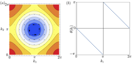
Figure 1: (a) The Siegel theta function $\mathcal{N}(\mathbf{k})$ (see Eq. (18)) is plotted with arrows denoting the vector field ${\cal A}_{nn}({\bf{k}})$. The winding in ${\cal A}$ around the zero located at $k_{1}=\pi,k_{2}=\pi$ leads to a Chern number in the basis states. (b) The Wilson loop $W(k_{1})=e^{i\theta(k_{1})}$ of a single Landau level integrated along $k_{2}$ is plotted as a function of $k_{1}$. The Wilson loop is computed analytically in App. A.7 to be $W(k_{1})=e^{-ik_{1}}$ (shown in solid blue) which winds once crossing the vortex at $(\pi,\pi)$. The numerical approximation of $W(k_{1})$ is dotted.

Our basis of magnetic translation eigenstates (Eq. (15)) is built from continuum Landau levels. These states are known to carry a Chern number Thouless et al. (1982), and it will be important to see how this arises in our formalism. To study the topology, we need to compute the continuum Berry connection:

$$(2\pi)^{2}\delta(\mathbf{k}-\mathbf{k}^{\prime})\mathcal{A}^{mn}(\mathbf{k}) =\braket{\mathbf{k}^{\prime},m}{\mathbf{r}}{\mathbf{k},n}\ .$$ (28)

In zero flux where the basis states are plane waves or Fourier transforms of localized orbitals, $\mathcal{A}^{mn}(\mathbf{k})$ would be trivial. However, the basis states at $2\pi$ flux are built out of Landau levels, which by themselves are topologically nontrivial. We can see this directly by computing $\braket{\mathbf{k}^{\prime},n}{\mathbf{r}}{\mathbf{k},n}$ (here the Landau level index $n$ is unsummed), the Abelian Berry connection of the $n$th Landau level, using the oscillator algebra. The result from App. A.7 is

$$\hbox{}\mathcal{A}^{nn}_{i}(\mathbf{k}) =-\frac{1}{2}\epsilon_{ij}\partial_{j}\log\vartheta\left(\left.\frac{(k_{1},k_{2})}{2\pi}\right|\Phi\right)$$ (29)

where $\partial_{i}=\frac{\partial}{\partial k_{i}}$ here for brevity, $\mathcal{A}_{i}=\mathbf{b}_{i}\cdot\mathcal{A}$, and we emphasize that $\mathcal{A}_{nn}(\mathbf{k})$ is independent of $n$. Interestingly, a similar formula has appeared recently in flat band Chern states in Ref. Wang et al. (2021). We now show that the connection Eq. (29) has Chern number $-1$. In App. A.7, we show with a direct computation that the Berry curvature is given by

$$\epsilon_{ij}\partial_{i}\mathcal{A}_{j}^{nn}=\frac{1}{2}\partial^{2}\log\vartheta=-\frac{1}{2\pi}+2\pi\delta(\mathbf{k}-\pi\mathbf{b}_{1}-\pi\mathbf{b}_{2})$$ (30)

and has two contributions. The $-1/2\pi$ term in Eq. (30) is the constant and nonzero Berry curvature of a Landau level Wang et al. (2021); Pfannkuche and Gerhardts (1992). The delta function appearing at $\mathbf{k}^{*}=\pi\mathbf{b}_{1}+\pi\mathbf{b}_{2}$ is an artifact of the undefined basis states at $\mathbf{k}^{*}$ where $\mathcal{N}(\mathbf{k}^{*})=0$ and is discussed fully in App. A.7. In fact, the $2\pi$ delta function is unobservable in the Wilson loop winding because the Berry phase is only defined mod $2\pi$. To see this, we explicitly calculate the Abelian Wilson loop (or Berry phase) in App. A.7 and show the result in Fig. 1(b) where we see that the Wilson loop eigenvalues are indeed continuous mod $2\pi$. Hence we can think of the the basis states in Eq. (15) as lattice-regularized Landau levels. We also see that the zero in the normalization factor $\mathcal{N}(\mathbf{k})$ (see Sec. III) is an essential feature of the basis rather than a pathological one: it is a manifestation of the topology of the basis states. If there were no zero, then we would have written down wavefunctions which were periodic and differentiable on the entire BZ, hence precluding a Chern number Brouder et al. (2007).

Finally, we obtain an explicit expression for the non-Abelian Berry connection $\mathcal{A}^{MN}(\mathbf{k})$ in the occupied bands indexed by $M,N$:

$$(2\pi)^{2}\delta(\mathbf{k}-\mathbf{k}^{\prime})\mathcal{A}^{MN}(\mathbf{k})\!=\!\sum_{mn}[U^{\dagger}(\mathbf{k}^{\prime})]^{M}_{m}\!\braket{\mathbf{k}^{\prime},m}{\mathbf{r}}{\mathbf{k},n}U_{n}^{N}(\mathbf{k})$$ (31)

where $U(\mathbf{k})$ is the $N_{LL}\times N_{occ}$ matrix of eigenvectors. $N_{occ}$ is the number of occupied bands and $N_{LL}$ is the dimension of the matrix Hamiltonian, which is truncated at $N_{LL}$ Landau levels. Leaving the details of the calculation to App. A.7, we give the general formula

$$\mathcal{A}_{i}^{MN}(\mathbf{k}) =[U^{\dagger}(i\partial_{i}-\epsilon_{ij}\tilde{Z}_{j})U]^{MN}$$ (32)

$$\qquad-\frac{\delta^{MN}}{2}\epsilon_{ij}\partial_{j}\log\vartheta\left(\left.\frac{(k_{1},k_{2})}{2\pi}\right|\Phi\right)\ .$$

The Abelian term in the second line of Eq. (32) describes the Chern numbers of the basis states as in Eq. (29). Note that it is proportional to the identity $\delta^{MN}$ and so can be factored out of the Wilson loop to give an overall winding factor per Landau level as shown in Fig. 1(b). The new non-Abelian term $U^{\dagger}\tilde{Z}_{j}U$ of Eq. (32) describes coupling between Landau levels where the Hermitian matrix $[\tilde{Z}_{j}]_{mn}=\braket{m}{Z_{j}}{n}$ is given in Eq. (27). Returning to Eq. (32), we write the non-Abelian Wilson loop as the path-ordered matrix exponential

$$\hbox{}[W_{\mathcal{C}}]^{MN} =\left[\exp\left(i\oint_{\mathcal{C}}d\mathbf{k}\cdot\mathcal{A}(\mathbf{k})\right)\right]^{MN}$$ (33)

$$=e^{-i\oint_{\mathcal{C}}d\mathbf{k}\times\frac{1}{2}\boldsymbol{\nabla}\log\vartheta\left(\left.\frac{(k_{1},k_{2})}{2\pi}\right|\Phi\right)}$$

$$\qquad\times\left[\exp\left(i\oint_{\mathcal{C}}dk_{i}\,U^{\dagger}(i\partial_{i}-\epsilon_{ij}\tilde{Z}_{j})U\right)\right]^{MN}$$

with a sum over $i,j$ implied. For numerical computations, Eq. (33) should be expanded into an ordered product form using the projectors $P_{\mathbf{k}}=U(\mathbf{k})U^{\dagger}(\mathbf{k})$. This procedure can be carried through exactly (the details may be found in App. A.7) and the result is

$$W_{\mathcal{C}} =\exp\left[-i\oint_{\mathcal{C}}d\mathbf{k}\times\frac{1}{2}\boldsymbol{\nabla}\log\vartheta\left(\left.\frac{(k_{1},k_{2})}{2\pi}\right|\Phi\right)\right]$$ (34)

$$\qquad\times U^{\dagger}(\mathbf{k}_{L})\mathcal{H}^{-d\mathbf{k}_{L}}\left(\prod_{n}^{(L-1)\leftarrow 1}P(\mathbf{k}_{n})\mathcal{H}^{-d\mathbf{k}_{n}}\right)U(\mathbf{k}_{0})$$

where $\mathcal{C}$ is a closed path with starting at $\mathbf{k}_{1}$ which is broken into $L$ segments labeled by $\mathbf{k}_{n}$, and $d\mathbf{k}_{n}=\mathbf{k}_{n}-\mathbf{k}_{n-1}$. The insertions of non-Abelian terms $\mathcal{H}^{d\mathbf{k}}=e^{i\epsilon_{ij}dk_{i}\tilde{Z}_{j}}$ act off-diagonally on the Landau level index (see Eq. (27)). The appearance of these non-Abelian terms reflects the fact that the Landau level states in Eq. (15) are not localized below the magnetic length, which is $1/\sqrt{\phi}$ in dimensionless units. In Sec. VI, we use the results of this section to calculate the Wilson loop in a square lattice model tuned through a topological phase transition at $2\pi$ flux by increasing the strength of the crystalline potential.

VI Square lattice Example

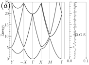
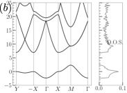
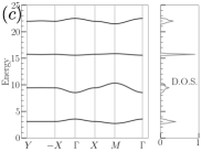
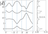
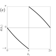
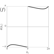
Figure 2: $\mathbf{(}a,b)$ Square lattice in zero flux, at low potential $w=1$ and high potential $w=7$ respectively. $\mathbf{(}c,d)$ Square lattice in $2\pi$ flux, at low potential and high potential respectively. $\mathbf{(}e,f)$ Wilson loops of the square lattice in flux. At low hoppings, the Hamiltonian resembles a Landau level system, resulting in nearly flat bands and a winding in the Wilson loop for the lowest band. At large hoppings, a gap closing occurs and allows the lowest band to have Chern number zero.

The simplicity of implementing our formalism is illustrated with a model of a scalar particle mass $m=1$ which feels a square lattice cosine potential. While it may be possible to simulate this type of model on an optical lattice Tarruell et al. (2012); Yılmaz et al. (2015); Aidelsburger et al. (2013), we intend this example to be pedagogical rather than physically motivated. We take the lattice vectors and reciprocal vectors to be ${\bf{a}}_{1}={\bf{b}}_{1}=(1,0),{\bf{a}}_{2}={\bf{b}}_{2}=(0,1)$ so $\Omega=1$ and define the zero-flux Hamiltonian as

$$H^{\phi=0}=-\frac{1}{2}{\boldsymbol{\nabla}}^{2}+\frac{w}{2}(e^{-2\pi i{\bf{b}}_{1}\cdot{\bf{r}}}+e^{-2\pi i{\bf{b}}_{2}\cdot{\bf{r}}}+H.c.),$$ (35)

where we have taken $\hbar=1$. When $w=0$, the Hamiltonian $H^{\phi=0}$ has continuous translation symmetry and solutions can be labeled by momentum ${\bf{k}}$. When $w$ is nonzero, the continuous translation symmetry is broken to a discrete symmetry which weakly couples the plane wave states and opens gaps at the corners of the BZ. By Bloch’s theorem, the states are labeled by momentum ${\bf{k}}$ in the BZ and the effective Hamiltonian reads

$$H^{\phi=0}_{\mathbf{G},\mathbf{G}^{\prime}}({\bf{k}}) =\frac{1}{2}({\bf{k}}-\mathbf{G})^{2}\delta_{\mathbf{G}\mathbf{G}^{\prime}}$$ (36)

$$\qquad+\frac{w}{2}(\delta_{\mathbf{G},\mathbf{G}^{\prime}-2\pi{\bf{b}}_{1}}+\delta_{\mathbf{G},\mathbf{G}^{\prime}-2\pi{\bf{b}}_{2}}+H.c.)$$

and $\mathbf{G}=G_{1}\mathbf{b}_{1}+G_{2}\mathbf{b}_{2},G_{i}\in\mathds{Z}$ (see App. B for details). We show the Bloch band structure in Fig. 2 in the weak and strong potential regimes. In flux, the Hamiltonian Eq. (35) is written in terms of the canonical momentum

$$H^{\phi}=\frac{1}{2}{\boldsymbol{\pi}}^{2}+\frac{w}{2}(e^{-2\pi i{\bf{b}}_{1}\cdot{\bf{r}}}+e^{-2\pi i{\bf{b}}_{2}\cdot{\bf{r}}}+H.c.),$$ (37)

that is, Landau levels in a lattice potential. In $2\pi$ flux using the matrix elements in Eq. 139 of Ref. SM , the magnetic Bloch Hamiltonian is

$$H^{\phi=2\pi}_{mn}(\mathbf{k}) =\phi(m+\frac{1}{2})\delta_{mn}$$ (38)

$$\qquad+\frac{w}{2}(e^{-ik_{2}}\mathcal{H}^{2\pi\mathbf{b}_{1}}_{mn}+e^{ik_{1}}\mathcal{H}^{2\pi\mathbf{b}_{2}}_{mn}+H.c.)$$

and recalling that the kinetic term acts on the $\ket{{\bf{k}},m}$ basis as $\frac{1}{2}\boldsymbol{\pi}^{2}=\phi(a^{\dagger}a+\frac{1}{2})$. The potential term $\mathcal{H}^{2\pi\mathbf{G}}_{mn}$ couples the Landau levels, giving nontrivial dispersion. We numerically calculate the band structure in the weak coupling ($w=1$) and strong coupling ($w=7$) regimes. The Landau level regime in weak coupling exhibits nearly flat bands (Fig. 2(c)), and its lowest band carries a Chern number, as exemplified by the winding of the Wilson loop shown in Fig. 2(e). Increasing $w$ pushes the model through a phase transition with a band touching at the $\Gamma$ point. At strong coupling ($w=7$), the $2\pi$ flux spectrum is gapped (Fig. 2(d)) and its lowest band has zero Chern number (Fig. 2(f)). Hence the lowest band cannot be interpreted as a Landau level, despite the strong flux.

VII Many-body Form Factors

Thus far, we have discussed the single-particle spectrum and Wilson loop topology of continuum Hamiltonians at $2\pi$ flux. In this section, we extend our formalism to many-body physics and derive a convenient expression for the Coulomb Hamiltonian

$$H_{int} =\frac{1}{2}\int d^{2}rd^{2}r^{\prime}\,n(\mathbf{r})V(\mathbf{r}-\mathbf{r}^{\prime})n(\mathbf{r}^{\prime})$$ (39)

in terms of the magnetic translation operator eigenbasis Eq. (15). Here $n(\mathbf{r})=c^{\dagger}(\mathbf{r})c(\mathbf{r})$ is the local density operator at $\mathbf{r}$ and $c(\mathbf{r}),c^{\dagger}(\mathbf{r})$ are the continuum fermion operators satisfying $\{c^{\dagger}(\mathbf{r}),c(\mathbf{r}^{\prime})\}=\delta(\mathbf{r}-\mathbf{r}^{\prime})$. In Sec. IX, we will project the Coulomb interaction on the flat bands of TBG in order to study its many-body insulating groundstates, as done in zero flux in Refs. Lian et al. (2021b); Bernevig et al. (2021a). The calculation for TBG is more involved because there are additional indices corresponding to valley and spin (see App. D.3 for details). For simplicity, we focus on models with only a single orbital per unit cell in this section and study the projected Coulomb Hamiltonian at $2\pi$ flux.

To avoid confusion with the Fock space braket notation in many-body calculations, we return to a wavefunction notation for the magnetic translation group eigenstates:

$$\psi_{{\bf{k}},n}(\mathbf{r})=\frac{1}{\sqrt{{\cal N}({\bf{k}})}}\sum_{\bf{R}}e^{-i{\bf{k}}\cdot{\bf{R}}}T_{\mathbf{a}_{1}}^{\mathbf{b}_{1}\cdot\mathbf{R}}T_{\mathbf{a}_{2}}^{\mathbf{b}_{2}\cdot\mathbf{R}}\frac{a^{\dagger n}}{\sqrt{n!}}\psi_{0}(\mathbf{r}),$$ (40)

where $\psi_{0}$ is the zeroth Landau level $a\psi_{0}=b\psi_{0}=0$. Throughout this section, $\ket{0}$ is the Fock vacuum satisfying $c(\mathbf{r})\ket{0}=0$ (not the Landau level vacuum) as is clear from context. The second-quantized creation operators $\psi_{{\bf{k}},n}^{\dagger}$ are defined by

$$\bra{\mathbf{r}}\psi_{{\bf{k}},n}^{\dagger}\ket{0}=\braket{0}{c_{\mathbf{r}}\psi_{{\bf{k}},n}^{\dagger}}{0}=\psi_{{\bf{k}},n}(\mathbf{r})$$ (41)

and $\{\psi_{{\bf{k}}^{\prime},m}^{\dagger},\psi_{{\bf{k}},n}\}=(2\pi)^{2}\delta_{mn}\delta(\mathbf{k}-\mathbf{k}^{\prime})$. We study the a general density-density interaction (essentially the Coulomb interaction with arbitrary screening) which can be put into the form

$$H_{int} =\frac{1}{2}\int d^{2}rd^{2}r^{\prime}\,n(\mathbf{r})V(\mathbf{r}-\mathbf{r}^{\prime})n(\mathbf{r}^{\prime})$$ (42)

$$=\frac{1}{2}\int\frac{d^{2}q}{(2\pi)^{2}}\,V(\mathbf{q})\rho_{-\mathbf{q}}\rho_{\mathbf{q}},\quad\rho_{\mathbf{q}}=\int d^{2}r\,e^{-i\mathbf{q}\cdot\mathbf{r}}n(\mathbf{r})$$

where $V(\mathbf{q})$ is the Fourier transform of the position-space potential. Throughout, we use $\mathbf{q}=\mathbf{k}+2\pi\mathbf{G}$ to denote a continuum momentum. We assume that $V(\mathbf{q})>0$ but is otherwise fully general. Our goal is to express the Fourier modes $\rho_{\mathbf{q}}$ in terms of the $\psi^{\dagger}_{\mathbf{k},m}$ operators. This is accomplished by calculating the matrix elements $\braket{0}{\psi_{\mathbf{k},m}\rho_{\mathbf{q}}\psi^{\dagger}_{\mathbf{k}^{\prime},n}}{0}$ because $\rho_{\mathbf{q}}$ is a one-body operator. The calculation is performed in App. C, and yields

$$\rho_{\bf{q}} =\sum_{mn}\int\dfrac{d^{2}k}{(2\pi)^{2}}e^{i\xi_{\bf{q}}({\bf{k}})}\psi_{{\bf{k}}-{\bf{q}},m}^{\dagger}{\cal H}^{\bf{q}}_{mn}\psi_{{\bf{k}},n},$$ (43)

with the phase factor $\xi_{\bf{q}}(\mathbf{k})$ defined by

$$e^{i\xi_{\bf{q}}({\bf{k}})}=\frac{e^{-\frac{\bar{q}q}{4\phi}}\vartheta\left(\left.\frac{(k_{1}-q/2,k_{2}+iq/2)}{2\pi}\right|\Phi\right)}{\sqrt{\vartheta\left(\left.\frac{(k_{1},k_{2})}{2\pi}\right|\Phi\right)\vartheta\left(\left.\frac{(k_{1}-q_{1},k_{2}-q_{2})}{2\pi}\right|\Phi\right)}}.$$ (44)

with $q=(\mathbf{a}_{1}+i\mathbf{a}_{2})\cdot\mathbf{q}$. The unitary matrix $\mathcal{H}^{\mathbf{q}}$ defined in Eq. (27). We prove analytically that $e^{i\xi_{\bf{q}}({\bf{k}})}$ is a pure phase at the end of App. A.6. At $\mathbf{k}=\pi\mathbf{b}_{1}+\pi\mathbf{b}_{2}$ and $\mathbf{k}=\pi\mathbf{b}_{1}+\pi\mathbf{b}_{2}+\mathbf{q}$, the denominator of Eq. (44) has zeroes which are exactly canceled by the zeros of the numerator (they are removable singularities), so $\xi_{\mathbf{q}}(\mathbf{k})$ is always real. We plot $\xi_{\mathbf{q}}(\mathbf{k})$ in Fig. 3 which shows that a branch cut connects the removable singularities at $(\pi,\pi)$ and $(\pi+q_{1},\pi+q_{2})$.

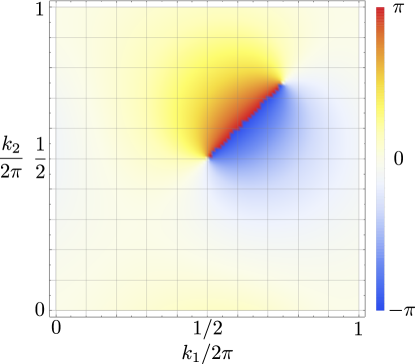
Figure 3: Phase $\xi_{\bf{q}}({\bf{k}})$ in Eq. 44 for ${\bf{q}}=\frac{\pi}{2}\mathbf{b}_{1}+\frac{\pi}{2}\mathbf{b}_{2}$, plotted as a density. Note the branch cut linking $(1/2,1/2)$ to $(3/4,3/4)$.

So far, we have developed an expression for the density operators (Eq. (43)) and thus for the many-body Coulomb Hamiltonian in terms of the single-particle magnetic translation group eigenstates. This will make it possible to perform a projection onto a set of low-energy bands. To do so, define the energy eigenstate operator $\gamma_{{\bf{k}},N}^{\dagger}$ that creates state at momentum ${\bf{k}}$ in band $N$:

$$\gamma_{{\bf{k}},N}^{\dagger}=\sum_{m}U^{N}_{m}({\bf{k}})\psi^{\dagger}_{{\bf{k}},m},$$ (45)

with $U^{N}(\mathbf{k})$ the eigenvector of the Hamiltonian corresponding to band $N$. (In models with more orbitals indexed by $\alpha$, Eq. (45) would also contain a sum over $\alpha$.) In second quantized notation, we arrive at the general expression

$$\rho_{\bf{q}}=\int\dfrac{d^{2}k}{(2\pi)^{2}}\sum_{MN}\gamma_{{\bf{k}}-{\bf{q}},M}^{\dagger}M_{MN}({\bf{k}},{\bf{q}})\gamma_{{\bf{k}},N},$$ (46)

where the form factor matrix $M(\mathbf{k},\mathbf{q})$ obtained from Eq. (46) is defined as

$$M_{MN}({\bf{k}},{\bf{q}})=e^{i\xi_{\bf{q}}({\bf{k}})}[U^{\dagger}({\bf{k}}-{\bf{q}}){\cal H}^{\bf{q}}U({\bf{k}})]_{MN}\ .$$ (47)

Note that $M(\mathbf{k},\mathbf{q})$ is not a gauge-invariant quantity because the eigenvectors in the matrices $U(\mathbf{k})$ and $U(\mathbf{k}-\mathbf{q})$ are only defined up to overall phases (or in general unitary transformations if there are degeneracies in the bands). App. D.3 contains a complete discussion, which we summarize by noting the “gauge freedom” taking $M(\mathbf{k},\mathbf{q})\to W^{\dagger}(\mathbf{k}-\mathbf{q})M(\mathbf{k},\mathbf{q})V(\mathbf{k})$ where $W(\mathbf{k}-\mathbf{q}),V(\mathbf{k})$ are arbitrary unitary matrices. There are gauge-invariant quantities determined from $M(\mathbf{k},\mathbf{q})$ such as its singular values, which are the eigenvalues of $M^{\dagger}(\mathbf{k},\mathbf{q})M(\mathbf{k},\mathbf{q})$. We will use the singular values to study the flat metric condition Bernevig et al. (2021b) in Sec. IX.1.

Having discussed the form factors, we emphasize that Eq. (46) is an exact expression for the density operator. To define a projected density operator, we restrict the indices $M,N$ to a subset of low-energy bands so that $\rho_{\mathbf{q}}$ annihilates all other bands. Our result in Eq. 46 is structurally similar to the form factor expression obtained in Ref. Bernevig et al. (2021b) in zero flux. We discuss the behavior of the form factor in App. D.3.

VIII Twisted Bilayer Graphene: Single-particle Physics

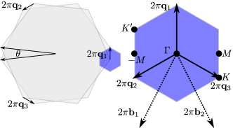
Figure 4: Construction and conventions of the moiré BZ, blue hexagon, from the graphene layers with relative twist $\theta$.

Twisted bilayer graphene (TBG) is a metamaterial formed from twisting two graphene sheets by a relative angle $\theta$ Bistritzer and MacDonald (2011a); Zou et al. (2018); Song et al. (2019). The resulting moiré pattern is responsible for the very large unit cell that allows experimental access to $\phi=2\pi$. Let us set our conventions for the geometry of the moiré twist unit cell. First, the graphene unit cell has a lattice vector of length $a_{g}=.246$nm and an area $\Omega_{g}=a_{g}^{2}\frac{\sqrt{3}}{2}$. The monolayer graphene K point is $\mathbf{K}_{g}=\frac{2\pi}{a_{g}}(0,2/3)$. The moiré vectors $\mathbf{q}_{j}$ are defined by the difference in momentum space of the rotated layers’ $K$ points:

$$2\pi\mathbf{q}_{1} =(R_{\theta/2}-R_{-\theta/2})\mathbf{K}_{g},\quad\mathbf{q}_{j}=C_{3}\mathbf{q}_{j-1},$$ (48)

$$2\pi|\mathbf{q}_{j}| \equiv k_{\theta}=2|\mathbf{K}_{g}|\sin\frac{\theta}{2}\,=\frac{8\pi\sin\frac{\theta}{2}}{3a_{g}}$$

where $R_{\theta}$ is a 2D rotation matrix. The moiré reciprocal lattice vectors are defined

$$\mathbf{b}_{j}=\mathbf{q}_{j}-\mathbf{q}_{3},\quad\mathbf{b}_{1}\times\mathbf{b}_{2} =\frac{(2\sin\frac{\theta}{2})^{2}}{\Omega_{g}}\ .$$ (49)

The moiré lattice is defined by $\mathbf{a}_{i}\cdot\mathbf{b}_{j}=\delta_{ij}$ which yields

$$\mathbf{a}_{1}=\frac{a_{g}}{2\sin\frac{\theta}{2}}\{-\frac{\sqrt{3}}{2},-\frac{1}{2}\}\quad\mathbf{a}_{2}=\frac{a_{g}}{2\sin\frac{\theta}{2}}\{\frac{\sqrt{3}}{2},-\frac{1}{2}\}\ .$$ (50)

Finally, the moiré unit cell has area

$$\Omega=\mathbf{a}_{1}\times\mathbf{a}_{2}=\frac{\Omega_{g}}{(2\sin\frac{\theta}{2})^{2}}\ .$$ (51)

The moiré Brillouin zone is depicted in Fig. 4. At the magic angle where $\theta=1.05^{\circ}$, the moiré unit cell is $\sim 3000$ times larger than the graphene unit cell. The magnetic translation group commutes when $\phi=\frac{eB\Omega}{\hbar}=2\pi$, which occurs at $B\in(25,32)$T for $\theta\in(1.03^{\circ},1.15^{\circ})$. These fields are experimentally accessible, making it possible to explore the Hofstadter regime of TBG. Ref. Herzog-Arbeitman et al. (2022) focuses on TBG at the magic angle, as well as the evolution of the spectrum in flux.

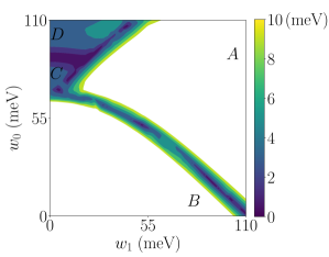
Figure 5: Phase diagram of TBG in $2\pi$ flux at magic angle. We plot the gap between the flat and passive bands as a function of parameters $w_{0},w_{1}$. Phase $A$, containing the physical TBG parameters is in the crystalline regime where the flat bands have zero Chern number, while phase $B$ is connected to the Landau level limit where each flat band has Chern number $-1$. The first chiral limit where $w_{0}$ is in phase $B$ at $w_{1}=110$meV. C and D are phases connected to the second chiral limit $w_{1}=0$ where the bands have strong dispersion (see Fig. 6).

The following sections contain a thorough treatment of TBG at $2\pi$ flux. We discuss the Bistritzer-MacDonald (BM) Hamiltonian in Sec. VIII.1 and show the phase diagram of TBG, identifying a crystalline regime (including the physical TBG parameters) where the flat bands have vanishing Chern number and a Landau level regime (including the first chiral limit) where the flat bands each have Chern number $-1$, denoted by $A$ and $B$ respectively in the phase diagram Fig. 5. In Sec. 7, we discuss the symmetries, topology, and Wannier functions which are different than at zero flux. Importantly, we find that the $C_{2z}\mathcal{T}$ symmetry, which is essential in protecting the nontrivial topology at $\phi=0$, is broken. At $\phi=2\pi$, we find that the TBG flat band structure can be obtained from atomic limits but still has Wannier functions pinned to the corners of the moiré unit cells. In Sec. VIII.3, we focus on the chiral limit of TBG where the chiral anomaly, a well-studied feature of relativistic gauge theory Fradkin (2021); Peskin (2018); Adler (1969); Bell and Jackiw (1969); Fujikawa and Suzuki (2004); Lapa (2019); Niemi and Semenoff (1986); Witten (2016); Qi and Zhang (2011), protects a pair of perfectly flat bands in TBG at all angles at $2\pi$ flux.

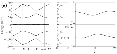
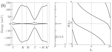
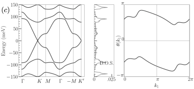
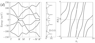
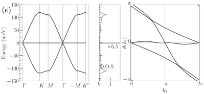
Figure 6: Band structures (left), density of states (middle), and Wilson loops (right) of TBG at $2\pi$ flux. The parameters $\big{(}\sqrt{3}w_{0}/(v_{F}k_{\theta}),\sqrt{3}w_{1}/(v_{F}k_{\theta})\big{)}$ given by (a): $(0.8,1)$, (b): $(0.05,0.8)$, (c): $(0.7,0.15)$, (d): $(0.97,0.32)$, (e): $(0.0,1.0)$. (a-d) are chosen to be connected to phases $A-D$ (see Fig. 5), and $(e)$, the chiral limit, is connected to $B$ but has a very small gap ($<2$meV). The very small gap makes the flat band Wilson loop ill-conditioned, so we compute the Wilson loop of the middle $4$ bands.

VIII.1 Band structure

We begin with the Bistritzer-MacDonald model of twisted bilayer graphene in the untwisted graphene $K$ valley (and arbitrary spin) at zero flux:

$$H_{BM}=\begin{pmatrix}-i\hbar v_{F}\boldsymbol{\sigma}\cdot\boldsymbol{\nabla}&T^{\dagger}({\bf{r}})\\ T({\bf{r}})&-i\hbar v_{F}\boldsymbol{\sigma}\cdot\boldsymbol{\nabla}\end{pmatrix},$$ (52)

with $\sigma$ labeling the sublattice degree of freedom and the $2\times 2$ matrix notation labeling the layer index. Note that $H_{BM}$ neglects the twist angle dependence in the kinetic term and thus has an exact particle-hole symmetry Song et al. (2019). For simplicity, we work in this approximation, but we note that incorporating the twist angle dependence poses no essential difficulty for our formalism. The moiré potential is $T({\bf{r}})=\sum_{j=1}^{3}e^{2\pi i{\bf{q}}_{j}\cdot{\bf{r}}}T_{j}$ where

$$T_{j+1}=w_{0}\sigma_{0} +w_{1}\left(\sigma_{1}\cos\frac{2\pi}{3}j+\sigma_{2}\sin\frac{2\pi}{3}j\right).$$ (53)

To add flux into $H_{BM}$, we employ the canonical substitution $-i\hbar\boldsymbol{\nabla}\rightarrow\boldsymbol{\pi}$. As written, $H_{BM}$ is not translation-invariant: the ${\bf{q}}_{i}$ vectors which appear in the moiré potential are not reciprocal lattice vectors. However, $H_{BM}$ can be made translation invariant by a unitary transformation:

$$V_{1}=\begin{pmatrix}e^{i\pi{\bf{q}}_{1}\cdot{\bf{r}}}&0\\ 0&e^{-i\pi{\bf{q}}_{1}\cdot{\bf{r}}}\end{pmatrix}$$ (54)

which acts only on the layer index. Acting on the states, $V_{1}$ shifts the momentum in the different layers by $2\pi\mathbf{q}_{1}$, reflecting separation of the Dirac points in Fig. 4. We then define the Hamiltonian in flux by

$$H^{\phi}_{BM}({\bf{r}})=V_{1}\begin{pmatrix}v_{F}\boldsymbol{\sigma}\cdot\boldsymbol{\pi}&T^{\dagger}({\bf{r}})\\ T({\bf{r}})&v_{F}\boldsymbol{\sigma}\cdot\boldsymbol{\pi}\end{pmatrix}V_{1}^{\dagger}$$ (55)

$$=\begin{pmatrix}v_{F}\boldsymbol{\sigma}\cdot\boldsymbol{\pi}-\pi v_{F}{\bf{q}}_{1}\cdot\boldsymbol{\sigma}&{\tilde{T}}^{\dagger}({\bf{r}})\\ {\tilde{T}}({\bf{r}})&v_{F}\boldsymbol{\sigma}\cdot\boldsymbol{\pi}+\pi v_{F}{\bf{q}}_{1}\cdot\boldsymbol{\sigma}\end{pmatrix}$$

with $\tilde{T}({\bf{r}})=T_{1}+T_{2}e^{2\pi i{\bf{b}}_{1}\cdot{\bf{r}}}+T_{3}e^{2\pi i{\bf{b}}_{2}\cdot{\bf{r}}}$. In this form, the matrix elements of $\tilde{T}({\bf{r}})$ in the magnetic translation operator basis can be directly obtained with Eq. 139 in Ref. SM in a sublattice/Landau level tensor product basis. An explicit expression is given in Eq. 228 of Ref. SM . The kinetic term can be expressed simply with Landau level operators. Expanding the Pauli matrices, we find

$$v_{F}\boldsymbol{\sigma}\cdot\boldsymbol{\pi} =v_{F}\sqrt{2eB}\begin{pmatrix}0&a^{\dagger}\\ a&0\end{pmatrix}=v_{F}\sqrt{2\phi/\Omega}\begin{pmatrix}0&a^{\dagger}\\ a&0\end{pmatrix}$$ (56)

$$=v_{F}k_{\theta}\left(\frac{3\sqrt{3}}{2\pi}\right)^{1/2}\begin{pmatrix}0&a^{\dagger}\\ a&0\end{pmatrix}$$

using $\phi=2\pi$ and the moiré wavevector $k_{\theta}$ in Eq. (48). The numerical factor coming from the unit cell geometry is $(3\sqrt{3}/2\pi)^{1/2}\simeq.91$. Lastly, the momentum shift $\pi v_{F}{\bf{q}}_{1}\cdot\boldsymbol{\sigma}$ in Eq. (LABEL:eq:BM2pi) acts as the identity on the Landau level index, and $\pi v_{F}{\bf{q}}_{1}\cdot\boldsymbol{\sigma}=\frac{v_{F}k_{\theta}}{2}\sigma_{2}$ using $2\pi\mathbf{q}_{1}=k_{\theta}\hat{y}$. The Dirac Hamiltonian Eq. (56) in flux is well-studied. At $2\pi$ flux and $\theta=1.05^{\circ}$, the low energy spectrum of Eq. (56) consists of a zero mode and states at $\pm E_{1}=\pm.91v_{F}k_{\theta}=\pm 170$meV. This is on the same scale as the potential strength $w_{1}=110$meV.

Numerical analysis of the band structure is straightforward and yields two flat bands (per valley and spin, or $8$ total) gapped from the dispersive bands by approximately 40 meV. See Fig. 6(a) for the band structure, density-of-states, and the Wilson loop of the flat bands for TBG, Fig. 6(b-e) for other choices of parameters $w_{0},w_{1}$. For a close-up of the flat-band dispersion at the magic angle see Fig. 7.

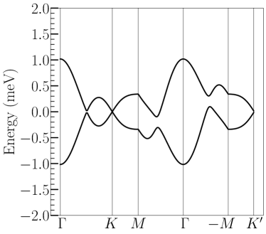
Figure 7: Close-up of the flat bands of TBG in flux at magic angle. Note the protected Dirac points at $K,K^{\prime}$ due to the different $C_{3}$ eigenvalues of the flat bands (see Eq. (59)) and $MT,P$ symmetries, as well as the maximal gap at $\Gamma$ where the $C_{3}$ eigenvalues are the same.

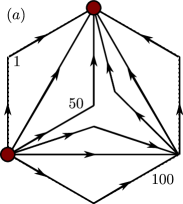
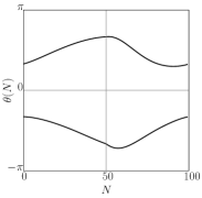
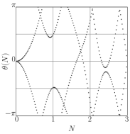
(c)

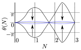
Figure 8: $C_{3}$-symmetric Wilson loops, discussed in Refs. Song et al. (2019); Bradlyn et al. (2019). In (a), the path 1 begins at $K$, goes to $K^{\prime}$, then back to $K$. The midpoint of the path is continuously changed until $\Gamma$ at $50$; further paths then follow a more complicated trajectory linking $K$ back to $K$ and then back again. In $(b)$, Wilson loops are taken in successively larger hexagons surrounding the $\Gamma$ point. Neither loop has nontrivial winding because there are no symmetries that protect crossings at $\pm\pi$, so the Wilson loops can be deformed to flat lines as depicted in $(c)$ which shows a caricature of the deformation process.

VIII.2 Symmetries and Topology

In zero flux, the topology of the TBG flat bands is protected by $C_{2z}\mathcal{T}$ symmetry Song et al. (2019, 2021); Bouhon et al. (2019). However, $C_{2z}\mathcal{T}$ is broken in nonzero flux because $\mathcal{T}$ reverses the magnetic field and $C_{2z}$ preserves it Herzog-Arbeitman et al. (2020). On the lattice in the Peierls approximation, $C_{2z}\mathcal{T}$ is restored as a (projective) symmetry at certain values of the flux Herzog-Arbeitman et al. (2020), but we do not consider this approximation here. In this section, we show that the band representation of TBG at $\phi=2\pi$ can be obtained from inducing atomic orbitals at the corners of the moiré unit cell, so the fragile topology at $\phi=0$ is broken by magnetic field. However, we find that band representation is decomposable Bradlyn et al. (2017); Cano et al. (2018a, b); Bradlyn et al. (2019), so the flat bands are topologically nontrivial when gapped from each other via a particle-hole breaking term.

First we review the topology in zero flux which is discussed comprehensively in Refs. Song et al. (2019, 2021). The space group of TBG is $p6^{\prime}2^{\prime}2$ which is generated by $C_{3},C_{2z}\mathcal{T},$ and $C_{2x}$. The symmetries are: three-fold rotations around the $AA$ moiré site $C_{3}$, spacetime inversion $C_{2z}\mathcal{T}$, and two-fold rotation around the $x$-axis $C_{2x}$. Note that in 2D, $C_{2x}$ is indistinguishable from $M_{y}$, a mirror taking $y\to-y$. The band representation of the flat bands is

$$\mathcal{B}^{\phi=0}=\Gamma_{1}+\Gamma_{2}+K_{2}K_{3}+M_{1}+M_{2}$$ (57)

and the irreps are defined at the high symmetry momenta $\Gamma=(0,0),K=2\pi\mathbf{q}_{1},M=\pi\mathbf{b}_{1}$ by

$$\begin{array}[]{c|ccc}6^{\prime}m^{\prime}m&1&C_{3}&M_{y}\\ \hline\cr\Gamma_{1}&1&1&1\\ \Gamma_{2}&1&1&-1\\ \end{array},\ \begin{array}[]{r|rr}6^{\prime}&1&C_{3}\\ \hline\cr K_{2}K_{3}&2&-1\\ \end{array},\ \begin{array}[]{c|cc}2^{\prime}m^{\prime}m&1&C_{2x}\\ \hline\cr M_{1}&1&1\\ M_{2}&1&-1\\ \end{array}\ .$$ (58)

The presence of the anti-unitary $C_{2z}\mathcal{T}$ ($PC_{2z}\mathcal{T}$) symmetry in the space group is required to prove that the band representation $\mathcal{B}^{\phi=0}$ is fragile (stable) topological Song et al. (2019, 2021).

At $2\pi$ flux, the $C_{2z}\mathcal{T}$ and $C_{2x}$ symmetries are broken because they reverse the magnetic field Herzog-Arbeitman et al. (2020). The resulting band topology is mentioned in Ref. Herzog-Arbeitman et al. (2022), which we review here for completeness. Without $C_{2z}\mathcal{T}$, the topology of the flat bands is not protected. The most direct way to see this is from the Wilson loop (see Eq. (33)) integrated along $\mathbf{b}_{2}$ in Fig. 8(a) which shows no relative winding. The same Wilson loop at zero flux has $C_{2z}\mathcal{T}$-protected relative winding Song et al. (2019). We also plot the $C_{3}$-symmetric Wilson loops discussed in Refs. Song et al., 2019; Bradlyn et al., 2019 and find no winding, as shown in Fig. 8(a,b). The lack of winding in any Wilson loop suggests that localized, symmetry-respecting Wannier states may be formed from the two TBG flat bands at $2\pi$ flux (per valley per spin) Bradlyn et al. (2017); Elcoro et al. (2020). Below, we discuss the flat bands in detail from the perspective of topological quantum chemistry.

At $2\pi$ flux, the 2D space group is reduced to $p31m^{\prime}$ (the $k_{z}=0$ plane of the 3D space group 157.55 in the BNS setting) generated by $C_{3}$ and $M\mathcal{T}\equiv C_{2x}C_{2z}\mathcal{T}$. The full algebra, including the anti-commuting unitary $P$ symmetry, is

$$M\mathcal{T}C_{3} =C^{\dagger}_{3}M\mathcal{T},~{}~{}C_{3}^{3}=1$$

$$[P,C_{3}] =0,~{}~{}P^{2}=-1$$

$$\{P,M\mathcal{T}\} =0~{}~{}(M\mathcal{T})^{2}=+1$$

and their action on the Hamiltonian is

$$C_{3}H^{\phi=2\pi}(\mathbf{k})C_{3}^{\dagger} =H^{\phi=2\pi}(C_{3}\mathbf{k}),$$ (59)

$$M\mathcal{T}H^{\phi=2\pi}(k_{x},k_{y})(M\mathcal{T})^{-1} =H^{\phi=2\pi}(k_{x},-k_{y}),$$

$$PH^{\phi=2\pi}(\mathbf{k})P^{\dagger} =-H^{\phi=2\pi}(-\mathbf{k}).$$

The operator ${\cal P}=PM\mathcal{T}$ squares to $+1$ and satisfies ${\cal P}C_{3}=C_{3}^{2}{\cal P}$. ${\cal P}$ sends $(k_{x},k_{y})\to(-k_{x},k_{y})$ and hence is local at the $K$ and $K^{\prime}$ points. Because ${\cal P}$ anticommutes with the Hamiltonian at $\Gamma,K$, and $K^{\prime}$, it switches the two flat bands if they are at nonzero energies $\pm E$. If ${\cal P}\ket{\Psi_{+E}}=\ket{\Psi_{-E}}$ and $\ket{\Psi_{+E}}$ carries $C_{3}$ eigenvalue $\omega$, then $\ket{\Psi_{-E}}$ also carries eigenvalue $\omega$. For the $\Gamma$ point this is indeed what happens – we find the $\Gamma$ point is gapped in Fig. 7 – but the $K,K^{\prime}$ points cannot gap, as a Dirac cone carries different $C_{3}$ eigenvalues in the two flat bands.

Ref. Herzog-Arbeitman et al. (2020) demonstrated that no symmetries or topology protect a gap closing between the flat bands and passive bands at nonzero flux, matched by experimental evidence in Refs. Das et al. (2022, 2021). As such, the irreps in nonzero flux are obtained from $\mathcal{B}^{\phi=0}$ by reduction to the $p31m^{\prime}$ subgroup of $p6^{\prime}2^{\prime}2$. We use the Bilbao Crystallographic Server Aroyo et al. (2006a, b) to determine the irreps and elementary band representations of $p31m^{\prime}$. They may be found at https://www.cryst.ehu.es/cgi-bin/cryst/programs/mbandrep.pl. The irreps of $p31m^{\prime}$ are very simple: the high symmetry momenta are $\Gamma,K$, and $K^{\prime}$ where all irreps are those of the point group $3$, so irreps at $\phi=0$ reduce to their $C_{3}$ eigenvalues at $\phi\neq 0$. We find

$$\mathcal{B}^{\phi=2\pi}=\mathcal{B}^{\phi=0}\downarrow p31m^{\prime}=2\Gamma_{1}+K_{2}+K_{3}+K^{\prime}_{2}+K^{\prime}_{3}$$ (60)

where the irreps in $p31m^{\prime}$ that appear in Eq. (60) are defined

$$\begin{array}[]{r|rr}3m^{\prime}&1&C_{3}\\ \hline\cr\Gamma_{1}&1&1\\ \end{array},\quad\begin{array}[]{r|rr}3&1&C_{3}\\ \hline\cr K_{2}&1&e^{\frac{2\pi i}{3}}\\ K_{3}&1&e^{-\frac{2\pi i}{3}}\\ \end{array},\quad\begin{array}[]{r|rr}3&1&C_{3}\\ \hline\cr K^{\prime}_{2}&1&e^{-\frac{2\pi i}{3}}\\ K^{\prime}_{3}&1&e^{\frac{2\pi i}{3}}\\ \end{array}\ .$$ (61)

As discussed, the particle-hole symmetry $\mathcal{P}$ ensures that the irreps at the $K$ and $K^{\prime}$ points are degenerate, so $K_{2}+K_{3}$ and $K_{2}^{\prime}+K_{3}^{\prime}$ should be thought of as co-irreps. We can induce $\mathcal{B}^{\phi=2\pi}$ from the elementary band representations of $p31m^{\prime}$:

$$\mathcal{B}^{\phi=2\pi}=A_{2b}\uparrow p31m^{\prime}$$ (62)

where $2b$ is the Wyckoff position consisting of the $M\mathcal{T}$-related corners of the moiré unit cell (the AB and BA positions shown in Fig. 9) and the two-dimensional $A$ irrep is two $s$ orbitals, i.e. the representation of $C_{3}$ is $\mathbb{1}_{2\times 2}$. From Eq. (62), we see that the band representation of TBG at $2\pi$ flux can be obtained from elementary band representations. This fact, coupled with the calculation of trivial Wilson loops, demonstrates the elementary band representation is not topological. Note that the unitary particle-hole symmetry $P$ acts as inversion in real space, and is implemented on the $A_{2b}$ irrep by exchanging the $s$ orbitals at AB and BA sites. Because there is no obstruction to locally realizing all symmetries of TBG at $2\pi$ flux, lattice model approaches Vafek and Kang (2021); Kang and Vafek (2018) can faithfully capture the the topology. However, although $\mathcal{B}^{\phi=2\pi}$ is an elementary band representation, the Bilbao crystallographic server reveals that it is decomposable into two topological bands with Chern numbers $\pm 1$ if the particle-hole symmetry $P$ is broken and the flat bands gap. This case is discussed in Ref. Herzog-Arbeitman et al. (2022).

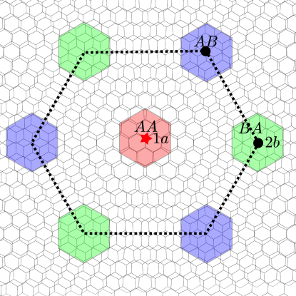
Figure 9: Moiré lattice in real space, with colored regions denoting the AA and AB, BA stacking regions. The band representation $\mathcal{B}^{\phi=2\pi}$ can be induced from $s$ orbitals at the 2b position, which is composed of the AB and BA moiré sites.

VIII.3 Chiral Anomaly in TBG

Ref. Tarnopolsky et al. (2019) first identified a special region in the TBG parameter space called the chiral limit where $w_{0}=0$ ($w_{1}$ is unrestricted). In the chiral limit, an anti-commuting symmetry $C=\tau_{0}\otimes\sigma_{3}\otimes\mathbb{1}$ ($\tau_{0}$ is the $2\times 2$ identity on the layer indices and $\mathbb{1}$ is the identity on the Landau level indices) appears which obeys

$$\{C,H_{BM}^{\phi}\}=0$$ (63)

for all flux $\phi$. We see this from Eq. 228 of Ref. SM because only $\sigma_{1}$ and $\sigma_{2}$ matrices appear when $w_{0}=0$ (see App. D.2). In zero flux, Ref. Tarnopolsky et al. (2019) identifies a discrete series of $w_{1}$ values where the two bands become exactly flat and have opposite chirality.

We now show that in chiral TBG at $2\pi$ flux, there are two exactly flat bands for all values of $w_{1}$, as we observe in Fig. 6(e). We will prove this is protected by the two flat bands having the same chirality. This is known as the chiral anomaly, which is a non-crystalline representation of chiral symmetry and cannot be realized in zero flux. First, recall that any state $\ket{E}$ at energy $E\neq 0$ yields a distinct state $\ket{-E}=C\ket{E}$ of energy $-E$, and the chiral eigenvalues on the basis $\ket{E},\ket{-E}$ are $\pm 1$ because they are exchanged by $C$. We can determine the chiral eigenvalues of the flat bands in TBG analytically in the small $w_{1}$ limit where the kinetic term dominates and

$$H^{\phi}_{BM}({\bf{r}})\to\begin{pmatrix}v_{F}\boldsymbol{\sigma}\cdot\boldsymbol{\pi}&0\\ 0&v_{F}\boldsymbol{\sigma}\cdot\boldsymbol{\pi}\end{pmatrix},\quad\text{as }w_{1}\to 0\ .$$ (64)

The eigenstates are in the form $(\ket{E_{n}},\pm\ket{E_{n}})^{T}$ where the $\pm$ states are orthogonal (so there are two states of energy $E_{n}$ to account for the two layers) and the Dirac Hamiltonian eigenstates are defined

$$\ket{E_{0}}=\begin{pmatrix}\ket{0}\\ 0\end{pmatrix},\quad\ket{E_{n}}=\frac{1}{\sqrt{2}}\begin{pmatrix}\ket{|n|}\\ \text{sgn}(n)\ket{|n|-1}\end{pmatrix},n\neq 0$$ (65)

with energies $\boldsymbol{\sigma}\cdot\boldsymbol{\pi}\ket{E_{n}}=\text{sgn}(n)\sqrt{2|n|\phi/\Omega}\ket{E_{n}}$ and $\text{sgn}(0)=0$. The chirality operator on the Dirac states obeys

$$\sigma_{3}\ket{E_{0}}=+\ket{E_{0}},\quad\sigma_{3}\ket{E_{n}}=\ket{E_{-n}}\ .$$ (66)

In the $w_{1}\to 0$ limit, the zero energy flat band eigenstates of $H_{BM}$ in the chiral limit are

$$\frac{1}{\sqrt{\mathcal{N}(\mathbf{k})}}\ \sum_{\mathbf{R}}e^{-i\mathbf{k}\cdot\mathbf{R}}T_{\mathbf{a}_{1}}^{\mathbf{b}_{1}\cdot\mathbf{R}}T_{\mathbf{a}_{2}}^{\mathbf{b}_{2}\cdot\mathbf{R}}\begin{pmatrix}\ket{E_{0}}\\ \pm\ket{E_{0}}\end{pmatrix}$$ (67)

at every $\mathbf{k}\in BZ$. The bands in Eq. (67) carry chiral eigenvalues $+1,+1$. Note that the chiral eigenvalues protect the perfectly flat bands at all $\mathbf{k}$: if the energy of either of the flat bands states was not exactly zero, then $C\ket{E}$ would be a distinct state and the pair would have chiral eigenvalues $\pm 1$. Hence the $+1,+1$ eigenvalues pin the states to zero energy. We now show this is true for $w_{1}\neq 0$. The proof is by contradiction. First, we increase $w_{1}$ away from zero so the flat band eigenstates are superpositions of many Landau levels. However, the chiral eigenvalues cannot change from $+1,+1$. All gap closings occur as states $\ket{\pm E}$ touch the zero energy flat bands, but a pair of states $\ket{\pm E}$ necessarily has chiral eigenvalues $\pm 1$ so the sum of the chiralities of the occupied bands is always $2$. Thus two states are always pinned to zero energy at every $\mathbf{k}$ and all $w_{1}$, yielding exactly flat bands at all angles. We emphasize that this situation is very different than at zero flux where the chiral eigenvalues of the flat bands are $\pm 1$ which allows them to gap at generic values of $w_{1}$.

The $+1,+1$ chiral eigenvalues are called the chiral anomaly because the trace of $C$ over all bands at fixed $\mathbf{k}$ formally satisfies

$$\text{Tr}\ \,C =\sum_{N=-\infty}^{\infty}U^{\dagger}_{N}(\mathbf{k})\sigma_{3}U_{N}(\mathbf{k})$$ (68)

$$=\sum_{N=\pm 1}U^{\dagger}_{N}(\mathbf{k})\sigma_{3}U_{N}(\mathbf{k})=2$$

which is anomalous because $\text{Tr}\ \sigma_{3}=0$. As in Eq. (45), $U_{N}(\mathbf{k})$ is the eigenvector of the $N$th band at momentum $\mathbf{k}$. In the second line of Eq. (68), we used the $\pm 1$ chiral eigenvalues of states at $E\neq 0$ to cancel them from the sum, leaving only the passive bands. The fact that $\text{Tr}\ C=2$ can be understood from the Atiyah-Singer index theorem Atiyah and Singer (1968); Eguchi et al. (1980) which states that each Dirac Hamiltonian contributes $\phi/(2\pi)$ to the trace of the chirality operator, so $\text{Tr}\ C=2$ at $\phi=2\pi$ because there are two layers Lapa (2019). Strictly speaking, we cannot apply the index theorem because we have constructed the spectrum on an infinite plane which is not compact. However, we can effectively compactify the spectrum by taking $\mathbf{k}$ to be discrete with $L^{2}$ values in the BZ corresponding to an $L\mathbf{a}_{1}\times L\mathbf{a}_{2}$ torus in real space. Then there are a total of $2L^{2}$ zero modes of $+1$ chirality from Eq. (68), so $\text{Tr}\ C=2$ at each $\mathbf{k}$.

We can also consider the second chiral limit of TBG identified in Ref. Bernevig et al. (2021b) where $w_{0}\neq 0$ and $w_{1}=0$. This limit has the chiral symmetry $C^{\prime}=\tau_{3}\sigma_{3}$ where $\tau_{3}$ is the Pauli matrix acting on the layer index. Numerically, we do not find zero-energy bands in the second chiral limit. This is because the Dirac zero modes in the top and bottom layers have opposite chiralities due to $\tau_{3}$, so there is no chiral anomaly to protect the exact flatness.

IX Twisted Bilayer Graphene: Many-body Physics

The rich single-particle physics of TBG at $2\pi$ flux, discussed at length in Sec. VIII, is characterized by the presence of low-energy flat bands. At the magic angle $\theta=1.05$, the theoretically predicted small bandwidth $\sim 2$meV means that the Coulomb interaction, which is $\sim 24$meV, is the dominant term in the TBG Hamiltonian Bernevig et al. (2021c). The large gap to the passive bands of $\sim 40$meV makes a strong coupling approximation viable where the Coulomb Hamiltonian is projected into the flat bands and the flat band kinetic energy is neglected. This strategy has been used to great effect in predicting the groundstate properties of TBG near zero flux Bernevig et al. (2021c); Lian et al. (2021b); Bernevig et al. (2021a); Kang and Vafek (2019); Kang et al. (2021); Ledwith et al. (2021).

Because the kinetic band energy is $<2$meV and the Zeeman spin splitting is also $\sim 2$meV at $30$T, it is consistent to neglect both terms in the Hamiltonian at $2\pi$ flux. In this case, a $U(4)$ symmetry emerges in the strong coupling approximation just like at $\phi=0$. Briefly, the spin and valley degeneracies act locally on the momentum $\mathbf{k}$ and lead to a $U(2)\times U(2)$ symmetry group, which is expanded in the strong coupling approximation to $U(4)$ by the operator $C_{2z}P$ which also acts locally on $\mathbf{k}$ (see App. D.2). Note that $C_{2z}P$ commutes with the Coulomb term in Eq. (42) but anti-commutes with the single-particle Hamiltonian $H_{0}$ which is why only the enhanced symmetry appears only in the strong coupling approximation where $H_{0}$ is set to zero in the flat bands. This is briefly reviewed in App. D.3 and explained in depth in Ref. Bernevig et al. (2021c).

We now apply the results of Sec. VII to TBG, setting the screened Coulomb interaction to

$$V(\mathbf{q})=\pi\xi^{2}U_{\xi}\frac{\tanh\xi|\mathbf{q}|/2}{\xi|\mathbf{q}|/2}$$ (69)

where the parameters of the screened Coulomb interaction are $\xi=10$nm, $U_{\xi}=e^{2}/(\epsilon\xi)=24$meV where $\epsilon$ is the dielectric constant Bernevig et al. (2021c).

IX.1 Many-body Insulator Eigenstates

Because the flat bands, approximate spin rotation, and valley symmetry survive the addition of $2\pi$ flux, one may add Coulomb interactions in the same manner as TBG in zero flux: by projecting density-density terms into the $8$ flat bands. These 8 bands have the creation operators $\gamma^{\dagger}_{\mathbf{k},M,\eta,s}$ where $M=\pm 1$ is the band, $\eta$ is the valley, and $s$ is the spin. We note that $\gamma^{\dagger}_{\mathbf{k}+2\pi\mathbf{G},M,\eta,s}=\gamma^{\dagger}_{\mathbf{k},M,\eta,s}$ because the eigenstates are periodic in $\mathbf{k}$ (see Sec. III.2). Just as in zero-flux, the density-density form of the Coulomb interaction in Eq. (42) (that has neither spin nor valley dependence) takes the positive-semidefinite form

$$H_{int}=\frac{1}{2\Omega_{tot}}\sum_{\mathbf{q}\in BZ}\sum_{\mathbf{G}}\,O_{-{\bf{q}},-\mathbf{G}}O_{{\bf{q}},\mathbf{G}},$$ (70)

where $\Omega_{tot}$ is the total area of the sample and the operators $O_{\mathbf{q},\mathbf{G}}=O^{\dagger}_{-\mathbf{q},-\mathbf{G}}$ are

$$O_{\mathbf{q},\mathbf{G}} =\sqrt{V(\mathbf{q}+2\pi\mathbf{G})}\sum_{\mathbf{k}\in BZ}\sum_{\eta,s}\sum_{MN}\bar{M}^{\eta}_{MN}(\mathbf{k},\mathbf{q}+2\pi\mathbf{G})$$

$$\qquad\times(\gamma^{\dagger}_{\mathbf{k}-\mathbf{q},M,\eta,s}\gamma_{\mathbf{k},N,\eta,s}-\frac{1}{2}\delta_{MN}\delta_{\mathbf{q},0})\ .$$ (71)

An expression for the form factor $\bar{M}^{\eta}_{MN}(\mathbf{k},\mathbf{q})$ is given in Eq. 282 of App. D. The term $\frac{1}{2}\delta_{MN}\delta_{\mathbf{q},0}$ is added to make $H_{int}$ symmetric about charge neutrality as in Ref. Bernevig et al. (2021c). To project in the flat bands, we merely restrict $M,N$ to the flat bands which we label $\pm 1$. If all flat band states of a given valley $\eta$ and spin $s$ are filled, $O_{{\bf{q}},\mathbf{G}}$ annihilates the state for all ${\bf{q}}\neq 0\text{ mod }2\pi\mathbf{G}$. This allows for the construction of exact eigenstates at filling $\nu=-4,-2,0,2,4$:

$$\ket{\Psi_{\nu}} =\prod_{\mathbf{k}}\prod_{j}^{(\nu+4)/2}\gamma^{\dagger}_{\mathbf{k},+,s_{j},\eta_{j}}\gamma^{\dagger}_{\mathbf{k},-,s_{j},\eta_{j}}\ket{0},$$ (72)

where $\gamma^{\dagger}_{{\bf{k}},\pm,s_{j},\eta_{j}}$ operators create flat band eigenstates with spin $s_{j}$ and valley $\eta_{j}$ which are arbitrary. Different choices of $j$ are related by $U(4)$ Lian et al. (2021b). The states $\ket{\Psi_{\nu}}$ all have zero Chern number because the two flat bands have no total winding (see Sec. 7). The operators $O_{\bf{q}}$ act simply on these states as calculated in App. D.4:

$$O_{\mathbf{q},\mathbf{G}}\ket{\Psi_{\nu}}=\delta_{\mathbf{q},0}\lambda_{\mathbf{G}}\ket{\Psi_{\nu}}$$ (73)

where ${\bf{q}}$ here is restricted to the BZ and

$$\lambda_{\mathbf{G}}=\nu\sqrt{V(2\pi\mathbf{G})}\sum_{\mathbf{k}\in BZ}\frac{1}{2}\text{Tr}\ \bar{M}(\mathbf{k},2\pi\mathbf{G})\ .$$ (74)

We prove in App. D.4 that $\bar{M}^{\eta}(\mathbf{k},2\pi\mathbf{G})$ and $\bar{M}^{-\eta}(\mathbf{k},2\pi\mathbf{G})$ are related by a unitary transform, so we drop the $\eta$ label on quantities which are independent of valley, such as $\text{Tr}\ \bar{M}^{\eta}(\mathbf{k},2\pi\mathbf{G})$. Appealing to Eq. (70), we show in App. D.4 that the energy of the eigenstates is

$$H_{int}\ket{\Psi_{\nu}} =\left(\frac{1}{2\Omega_{tot}}\sum_{\mathbf{G}}|\lambda_{\mathbf{G}}|^{2}\right)\ket{\Psi_{\nu}}$$ (75)

which vanishes at the charge neutrality point $\nu=0$ because $\lambda_{\mathbf{G}}\propto\nu$. Because $H_{int}$ is positive semi-definite, $\ket{\Psi_{0}}$ must be a groundstate because it has zero energy at $\nu=0$. Additionally, the $\nu=\pm 4$ eigenstates are trivially groundstates because they are fully filled/fully empty. Whether the $\ket{\Psi_{\nu}}$ are true groundstates for $\nu=\pm 2$ is still in question. One way to assess the groundstates at $\nu=2$ is with the flat metric condition Bernevig et al. (2021b), which is the approximation

$$\bar{M}^{\eta}(\mathbf{k},2\pi\mathbf{G})=m_{\mathbf{G}}\mathbb{1}_{2\times 2},$$ (76)

in other words that $\bar{M}(\mathbf{k},2\pi\mathbf{G})$ is multiple of the identity matrix which does not depend on $\mathbf{k}$ at each $\mathbf{G}$. In Ref. Lian et al. (2021b) it was shown that if the flat metric condition is satisfied, then $\ket{\Psi_{\nu}}$ are necessarily groundstates. App. D.4 contains a detailed review of this claim. In Fig. 10, we numerically calculate the singular values of $M(\mathbf{k},2\pi\mathbf{G})$ as in Ref. Lian et al. (2021b) and argue that Eq. (76) holds to a high degree of accuracy for all $2\pi|\mathbf{G}|\neq\sqrt{3}k_{\theta}$, as is also the case at $\phi=0$. For six $\mathbf{G}$ momenta $\pm\mathbf{b}_{1},\pm\mathbf{b}_{2},\pm(\mathbf{b}_{1}-\mathbf{b}_{2})$ where $2\pi|\mathbf{G}|=\sqrt{3}k_{\theta}$, the flat metric condition is still an acceptable approximation to an accuracy in energy of $\Omega^{-1}V(2\pi\sqrt{3}k_{\theta})\sim 10$meV times a numerical $O(1)$ constant depending on the violation of Eq. (76). From Eq. (10), the difference of the eigenvalues of $M^{\dagger}(\mathbf{k},2\pi\mathbf{G})M(\mathbf{k},2\pi\mathbf{G})$ is $\lesssim.33$, whereas if the flat metric condition held, the difference would be zero. Hence we estimate that the flat metric condition holds within $\Omega^{-1}V(2\pi\sqrt{3}k_{\theta})\times\sqrt{.33}\sim 5$meV. Unless states other than $\ket{\Psi_{\nu}}$ are very competitive in energy, we can assume that $\ket{\Psi_{\nu}}$ is a groundstate at $\nu=\pm 2$. The excitation spectrum above these ground states at $2\pi$ flux is studied in Ref. Herzog-Arbeitman et al. (2022). Ref. Wang and Vafek (2021) uses a complimentary technique to study the strong coupling excitations in small magnetic fields.

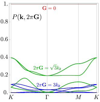
Figure 10: The validity of the flat metric condition can be evaluated by examining the eigenvalues of $P(\mathbf{k},2\pi\mathbf{G})=M^{\dagger}(\mathbf{k},2\pi\mathbf{G})M(\mathbf{k},2\pi\mathbf{G})$ as a function of $\mathbf{k}$. At $\mathbf{G}=0$ (red), $M(\mathbf{k},0)=U^{\dagger}(\mathbf{k})U(\mathbf{k})$ is the identity matrix so the flat metric condition is exactly satisfied. Because the form factor $M(\mathbf{k},2\pi\mathbf{G})$ decays exponentially in $\mathbf{G}$, the flat metric condition is very nearly true for $|\mathbf{G}|\geq 3$ (blue) because the eigenvalues are quite small. Thus the validity of the flat metric condition is determined to very good approximation by only the first momentum shell composed of $\mathbf{G}=\pm\mathbf{b}_{1},\pm\mathbf{b}_{2},\pm(\mathbf{b}_{1}-\mathbf{b}_{2})$ (green). We see that, while $M(\mathbf{k},2\pi\mathbf{G})$ is not proportional to the identity, the differences between the eigenvalues of $P(\mathbf{k},2\pi\mathbf{G})$ are $\lesssim.33$ which is only a small violation of the flat metric condition. We used the parameters $\theta=1.05$ and $w_{0}=.8w_{1}$, but we checked that the flat metric condition is reliable over a range of parameters.

X Discussion

The techniques developed in this paper allow for an analysis of general periodic Hamiltonians in $2\pi$ flux — most notably the continuum models of moiré meta-materials — generalizing Bloch’s theorem in a way that allows theoretical access to non-Peierls physics. We derived formulae for matrix elements, Wilson loops and Berry curvature, and projected density-density interactions. These tools expand the reach of modern topological band theory to the strong flux limit, opening Hofstadter topology to analytical and numerical study in the continuum.

Using these techniques, we build a physical picture of twisted bilayer graphene in $2\pi$ flux — a tantalizing experimental setup as the large moiré unit cell allows for laboratory access to the Hofstadter limit for intermediate and large flux Das et al. (2022); Yu et al. (2021). We find that in magic angle twisted bilayer graphene, the flat bands are reenter at $2\pi$ flux after splitting and broadening into Hofstadter bands at intermediate flux. The chiral limit of TBG, although physically inaccessible, showcases the chiral anomaly and exemplifies the non-crystalline properties of Hofstadter phases.

A natural development of this work is the extension of our gauge-invariant method to study the topology of band structures at general rational flux, which we pursue in future work. Such a development would be a powerful tool to study non-Peierls physics in topological magnetic systems, particularly with the ability to perform gauge-invariant Wilson loop calculations within our formalism. Investigations of strongly correlated phases like superconductivity and the fractional quantum hall effect are also made possible due to our expressions for the form factors.

During the preparation of this work, Ref. Sheffer and Stern (2021) independently studied the chiral limit in magnetic field. They find exact eigenstates for the zero-energy flat bands protected by chiral symmetry at all flux, but their techniques do not generalize to non-chiral Hamiltonians. We identify the same phase transition in Fig. 6(e) as described in their work.

XI Acknowledgements

We thank Zhi-Da Song and Dmitri Efetov for their insight. B.A.B. and A.C. were supported by the ONR Grant No. N00014-20-1-2303, DOE Grant No. DESC0016239, the Schmidt Fund for Innovative Research, Simons Investigator Grant No. 404513, the Packard Foundation, the Gordon and Betty Moore Foundation through Grant No. GBMF8685 towards the Princeton theory program, and a Guggenheim Fellowship from the John Simon Guggenheim Memorial Foundation. Further support was provided by the NSF-MRSEC Grant No. DMR-1420541 and DMR-2011750, BSF Israel US foundation Grant No. 2018226, and the Princeton Global Network Funds. JHA is supported by a Marshall Scholarship funded by the Marshall Aid Commemoration Commission.

Supplementary Material for “Magnetic Bloch Theorem and Reentrant Flat Bands in Twisted Bilayer Graphene at $2\pi$ Flux”

The following Appendices provide self-contained, detailed calculations for readers interested in the theoretical developments described in the Main Text. Alternatively, the important computational results are highlighted for readers wishing to simply make use of the formalism. We provide a brief outline of the Appendices and summarize the final results below.

App. A fully develops the gauge-invariant formalism of the magnetic Bloch theorem at $2\pi$ flux. App. A.1 defines the Landau level and guiding center operators. App. A.2 defines the magnetic translation group irreps. App. A.3 introduces the Siegel theta function and relevant identities. App. A.4 proves an important holomorphic/anti-holomorphic factorization formula for the Siegel theta function appearing in the basis states. App. A.5 discusses the completeness of the magnetic translation group irrep basis states. App. A.6 provides general formulas for the matrix elements of the magnetic Bloch Hamiltonian. App. A.7 contains an expression for the non-Abelian Wilson loop.

App. B exemplifies the magnetic Bloch formalism with a simple Hamiltonian. App. B.1 reviews Bloch’s theorem at zero flux, and App. B.2 analogously discusses the magnetic Bloch theorem at $2\pi$ flux.

App. C develops a gauge-invariant formula for the Coulomb interaction and an expression for the many-body form factors.

App. D applies the magnetic Bloch theorem to Twisted Bilayer Graphene. App. D.1 defines the conventions of the Bistritzer-MacDonald Hamiltonian. App. D.2 discusses the symmetries of the continuum model in magnetic flux. App. D.3 reviews the strong coupling expansion used to study the many-body physics. App. D.4 derives exact many-body groundstates at even integer fillings.

Appendix A Ladder Operator Calculations and the Siegel Theta function

In this Appendix, we define the operators and special functions used to derive the magnetic Bloch theorem at $2\pi$ flux. This section is technical, and the important results are highlighted for the convenience of readers. App. A.1 contains a derivation of the symmetry operators in flux. In App. A.2, we prove a central formula for the magnetic translation operator eigenstates. The Siegel theta function, a generalization of the Jacobi theta function, arises in this construction and is discussed in App. A.3. In App. A.4, we derive a simple expression (related to the Green’s function of the Laplacian on the torus) for the Siegel theta function appearing as a normalization factor. With this result, we then prove the completeness of the magnetic translation group irreps in App. A.5. Moving on to the spectrum, we then prove a general formula for the scattering amplitude between eigenstates in App. A.6 which is used to compute the magnetic Bloch Hamiltonian and many-body form factors. Finally, App. A.7 derives expressions for the non-Abelian Berry connection and demonstrates that the Landau levels forming the basis carry nonzero Chern numbers.

A.1 Operator Definitions

First, we must set our index conventions. We sum over repeated indices and use greek letters $\mu,\nu,\rho,\sigma$ for cartesian indices and roman letters $i,j,k,l$ for the crystalline indices of the lattice vectors $\mathbf{a}_{i}$. For instance, the reciprocal lattice vectors $\mathbf{b}_{i}$ are defined by $\mathbf{a}_{i}\cdot\mathbf{b}_{j}=\delta_{ij}$, where we used the dot product as a shorthand for contracting the cartesian indices of the vectors $\mathbf{a}_{i},\mathbf{b}_{i}$.

We recall the definitions of the canonical momentum and ladder operators defined in Sec. II of the Main Text. The canonical momentum with $\hbar=1$ is $\boldsymbol{\pi}=-i\boldsymbol{\nabla}-e\mathbf{A}$ obeying

$$\hbox{}[\pi_{\mu},\pi_{\nu}]=ie(\partial_{\mu}A_{\nu}-\partial_{\nu}A_{\mu})=ieB\epsilon_{\mu\nu}$$ (77)

and the Landau level ladder operators $[a,a^{\dagger}]$ are defined

$$a =\frac{\pi_{x}+i\pi_{y}}{\sqrt{2eB}},a^{\dagger}=\frac{\pi_{x}-i\pi_{y}}{\sqrt{2eB}}\quad\implies\quad\pi_{x}=\sqrt{\frac{eB}{2}}(a^{\dagger}+a),\pi_{y}=i\sqrt{\frac{eB}{2}}(a^{\dagger}-a)\ .$$ (78)

The guiding center momenta $Q_{\mu}$ are defined in a gauge-invariant way by

$$Q_{\mu} =\pi_{\mu}-eB\epsilon_{\mu\nu}x_{\nu}=-i\partial_{\mu}-e(A_{\mu}+B\epsilon_{\mu\nu}x_{\nu})\ .$$ (79)

We note that $Q_{\mu}=A_{\mu}+B\epsilon_{\mu\nu}x_{\nu}$ can be interpreted as the canonical momentum corresponding to a system with opposite magnetic field $-B$. At zero flux, where the time-reversal is not broken, $Q_{\mu}$ and $\pi_{\mu}$ are identical (up to a gauge choice). We will make frequent use of the simple identity

$$(eB)^{-1}\epsilon_{\mu\nu}(Q_{\nu}-\pi_{\nu})=-\epsilon_{\mu\nu}\epsilon_{\nu\rho}x_{\rho}=x_{\mu}$$ (80)

which gives a gauge-independent formula for $x_{\mu}$. The guiding center operators commute with the canonical momenta and obey

$$\hbox{}[Q_{\mu},\pi_{\nu}] =[\pi_{\mu}-eB\epsilon_{\mu\rho}x_{\rho},\pi_{\nu}]=ieB\epsilon_{\mu\nu}-ieB\epsilon_{\mu\nu}=0$$ (81)

$$[Q_{\mu},Q_{\nu}] =[\pi_{\mu}-eB\epsilon_{\mu\rho}x_{\rho},\pi_{\nu}-eB\epsilon_{\nu\sigma}x_{\sigma}]=-ieB\epsilon_{\mu\nu}\ .$$

The guiding centers form a separate oscillator system with $[b,b^{\dagger}]=1$ defined by

$$b =\frac{(\mathbf{a}_{1}-i\mathbf{a}_{2})\cdot\mathbf{Q}}{\sqrt{2\phi}},\quad b^{\dagger}=\frac{(\mathbf{a}_{1}+i\mathbf{a}_{2})\cdot\mathbf{Q}}{\sqrt{2\phi}}\quad\implies\quad\sqrt{\phi/2}(b+b^{\dagger})=\mathbf{a}_{1}\cdot\mathbf{Q},\ i\sqrt{\phi/2}(b-b^{\dagger})=\mathbf{a}_{2}\cdot\mathbf{Q}\ .$$ (82)

To prove $[b,b^{\dagger}]=1$, it is useful to note $[\mathbf{a}_{1}\cdot\mathbf{Q},\mathbf{a}_{2}\cdot\mathbf{Q}]=-ieB\mathbf{a}_{1}\times\mathbf{a}_{2}=-i\phi$. From Eq. (81), we have $[a,b]=[a^{\dagger},b]=[a,b^{\dagger}]=[a^{\dagger},b^{\dagger}]=0$. Because $a,b$ commute, we can find simultaneous eigenstates of $a^{\dagger}a$ and $b^{\dagger}b$. In particular, they have a simultaneous groundstate $\ket{0}$ satisfying $a\ket{0}=b\ket{0}=0$.

We define the magnetic translation operators to be

$$T_{\mathbf{a}_{i}} =\exp(i\mathbf{a}_{i}\cdot\mathbf{Q})$$ (83)

which obey the projective algebra

$$T_{\mathbf{a}_{1}}T_{\mathbf{a}_{2}} =\exp\Big{(}[i\mathbf{a}_{1}\cdot\mathbf{Q},i\mathbf{a}_{2}\cdot\mathbf{Q}]\Big{)}T_{\mathbf{a}_{2}}T_{\mathbf{a}_{1}}=e^{i\phi}T_{\mathbf{a}_{2}}T_{\mathbf{a}_{1}}$$ (84)

obtained using the Baker-Campbell-Hausdorff (BCH) identity $\exp X\exp Y=\exp([X,Y])\exp Y\exp X$ when $[X,Y]$ is a $c$-number: since $[[Q_{\mu},Q_{\nu}],Q_{\gamma}]=0$ for all $\mu,\nu,\gamma$, higher-order commutators in the BCH formula disappear. Lastly, it is also useful to define the gauge-invariant angular momentum operator

$$L_{z}=\frac{\mathbf{Q}^{2}-\boldsymbol{\pi}^{2}}{2eB}\ .$$ (85)

This choice is convenient because it decouples the $a$ and $b$ oscillators. To motivate the form of Eq. (85), we check that

$$\frac{\mathbf{Q}^{2}-\boldsymbol{\pi}^{2}}{2eB} =\frac{1}{2eB}(Q_{\mu}-\pi_{\mu})(\pi_{\mu}+Q_{\mu})$$ (86)

$$=-\frac{1}{2}\epsilon_{\mu\rho}x_{\rho}(2\pi_{\mu}-eB\epsilon_{\mu\sigma}x_{\sigma})$$

$$=\epsilon_{\mu\nu}x_{\mu}(-i\partial_{\nu})+e\epsilon_{\mu\rho}x_{\rho}\left[A_{\mu}+\frac{B}{2}\epsilon_{\mu\sigma}x_{\sigma}\right]$$

and the term in brackets is pure gauge (curl-free), i.e. $\epsilon_{\mu\nu}\partial_{\mu}(A_{\nu}+\frac{B}{2}\epsilon_{\nu\sigma}x_{\sigma})=0$. Thus in the symmetric gauge $A_{\mu}=-\frac{B}{2}\epsilon_{\mu\nu}x_{\nu}$ where $\pi_{\mu}=-i\partial_{\mu}+\frac{eB}{2}\epsilon_{\mu\nu}x_{\nu},Q_{\mu}=-i\partial_{\mu}-\frac{eB}{2}\epsilon_{\mu\nu}x_{\nu}$, we find

$$\frac{\mathbf{Q}^{2}-\boldsymbol{\pi}^{2}}{2eB} =\epsilon_{\mu\nu}x_{\mu}(-i\partial_{\nu})$$ (87)

which is the canonical angular momentum operator. We now check the algebra of rotations with the magnetic translation operators. These results will be useful when we derive the real-space form of the symmetry operators in flux. The first identity we need is

$$\hbox{}[\mathbf{Q}^{2},Q_{\mu}]=Q_{\nu}[Q_{\nu},Q_{\mu}]+[Q_{\nu},Q_{\mu}]Q_{\nu}=2eBi\epsilon_{\mu\nu}Q_{\nu}$$ (88)

which leads to

$$\left([\frac{\mathbf{Q}^{2}}{2eB},\right)^{n}Q_{\mu}] =(i\epsilon_{\mu\mu_{1}})(i\epsilon_{\mu_{1}\mu_{2}})\dots(i\epsilon_{\mu_{n-1}\mu_{n}})Q_{\mu_{n}}$$ (89)

$$\left([\frac{\mathbf{Q}^{2}}{2eB},\right)^{n}\mathbf{Q}] =\sigma_{2}^{n}\mathbf{Q}$$

where $\sigma_{2}$ is the Pauli matrix acting on the $\mu,\nu$ indices. Defining $([A,)^{n}B]=[A,[A,\cdots[A,B]]],$ and using an alternate version of BCH:

$$e^{X}e^{Y}e^{-X}=e^{Y+[X,Y]+\frac{1}{2!}[X,[X,Y]]\dots}$$ (90)

we perform the following calculation using Eq. (89):

$$e^{i\theta L_{z}}T_{{\bf{R}}}e^{-i\theta L_{z}} =e^{i\theta L_{z}}\exp[i{\bf{R}}\cdot\mathbf{Q}]e^{-i\theta L_{z}}$$ (91)

$$=\exp\sum_{n=0}^{\infty}\frac{1}{n!}\big{(}[i\theta\frac{\mathbf{Q}^{2}}{2eB},\big{)}^{n}i{\bf{R}}\cdot\mathbf{Q}]$$

$$=\exp\sum_{n=0}^{\infty}\frac{1}{n!}(i\theta)^{n}i{\bf{R}}\cdot\big{(}[\frac{\mathbf{Q}^{2}}{2eB},\big{)}^{n}\mathbf{Q}]$$

$$=\exp\sum_{n=0}^{\infty}\frac{1}{n!}(i\theta)^{n}i{\bf{R}}\cdot\sigma_{2}^{n}\mathbf{Q}$$

$$=\exp\left(i{\bf{R}}\cdot R_{-\theta}\mathbf{Q}\right)$$

$$=T_{R_{\theta}{\bf{R}}}\ .$$

This result shows that the algebra of rotations with translations is the same as at zero flux. Trivially, $[L_{z},\boldsymbol{\pi}^{2}]=0$, so $L_{z}$ commutes with the scalar kinetic term. For a Dirac-type Hamiltonian, we compute directly

$$\hbox{}[L_{z}+\frac{1}{2}\sigma_{3},\pi_{\mu}\sigma_{\mu}] =[-\frac{\boldsymbol{\pi}^{2}}{2eB}+\frac{1}{2}\sigma_{3},\pi_{\mu}\sigma_{\mu}]$$ (92)

$$=i\epsilon_{\mu\nu}\pi_{\nu}\sigma_{\mu}+i\epsilon_{\mu\nu}\pi_{\mu}\sigma_{\nu}=0$$

which shows that $L_{z}+\frac{1}{2}\sigma_{3}$ is the conserved angular momentum, appropriate for a particle with Berry phase. Finally, we need the action of functions of $\mathbf{r}$ to show that $L_{z}$ commutes with rotationally symmetric potential terms. We use

$$\hbox{}[L_{z},x_{\mu}] =\frac{1}{eB}\epsilon_{\mu\nu}[L_{z},Q_{\nu}-\pi_{\nu}]$$ (93)

$$=\frac{1}{2(eB)^{2}}\epsilon_{\mu\nu}([\mathbf{Q}^{2},Q_{\nu}]+[\boldsymbol{\pi}^{2},\pi_{\nu}])$$

$$=\frac{1}{eB}\epsilon_{\mu\nu}(i\epsilon_{\nu\rho}Q_{\rho}-i\epsilon_{\nu\rho}\pi_{\rho})$$

$$=\frac{1}{eB}\epsilon_{\mu\nu}(i\epsilon_{\nu\rho}(Q_{\rho}-\pi_{\rho}))$$

$$=i\epsilon_{\mu\nu}x_{\nu}$$

which is the same action as the canonical angular momentum $[\epsilon_{\nu\rho}x_{\nu}(-i\partial_{\rho}),x_{\mu}]=-i\epsilon_{\nu\mu}x_{\mu}$. Hence a $C_{n}$-symmetric potential at $B=0$ is also symmetric under rotations by Eq. (85) in nonzero magnetic field. This is just the classical statement that a perpendicular magnetic field does not break rotation symmetry.

A.2 Eigenstate Normalization

The calculation of the basis states in Eq. (15) of the Main Text is straightforward but involved. To streamline the notation, we use $\ket{n}=\frac{1}{\sqrt{n!}}a^{{\dagger}n}\ket{0}$ to denote the Landau level wavefunctions, which obey $a\ket{0}=b\ket{0}=0$ and $\braket{m}{n}$. The magnetic translation eigenstates are

$$\boxed{\ket{\mathbf{k},n}=\frac{1}{\sqrt{\mathcal{N}(\mathbf{k})}}\sum_{\mathbf{R}}e^{-i\mathbf{k}\cdot\mathbf{R}}T_{\mathbf{a}_{1}}^{\mathbf{R}\cdot\mathbf{b}_{1}}T_{\mathbf{a}_{2}}^{\mathbf{R}\cdot\mathbf{b}_{2}}\ket{n}}$$ (94)

and $T_{\mathbf{a}_{i}}=e^{i\mathbf{a}_{i}\cdot\mathbf{Q}}$. We have defined ${\bf{R}}=R_{1}\mathbf{a}_{1}+R_{2}\mathbf{a}_{2}$ for $R_{i}\in\mathds{Z}$.

All calculations can be performed with the BCH identity $\exp X\exp Y=\exp(\frac{1}{2}[X,Y])\exp(X+Y)$ when $[X,Y]$ is a $c$-number. We also set $\phi=2\pi$. The first step is

$$T_{\mathbf{a}_{1}}^{\mathbf{R}\cdot\mathbf{b}_{1}}T_{\mathbf{a}_{2}}^{\mathbf{R}\cdot\mathbf{b}_{2}} =e^{iR_{1}\mathbf{a}_{1}\cdot\mathbf{Q}}e^{iR_{2}\mathbf{a}_{2}\cdot\mathbf{Q}}=e^{i\mathbf{R}\cdot\mathbf{Q}+i\frac{\phi}{2}R_{1}R_{2}}=e^{i\mathbf{R}\cdot\mathbf{Q}+i\frac{\phi}{2}(\mathbf{R}\cdot\mathbf{b}_{1})(\mathbf{R}\cdot\mathbf{b}_{2})}$$ (95)

using $[\mathbf{a}_{1}\cdot\mathbf{Q},\mathbf{a}_{2}\cdot\mathbf{Q}]=-i\phi$. Hence we can write our states

$$\ket{\mathbf{k},n}=\frac{1}{\sqrt{\mathcal{N}(\mathbf{k})}}\sum_{\mathbf{R}}e^{-i\mathbf{k}\cdot\mathbf{R}+i\frac{\phi}{2}(\mathbf{R}\cdot\mathbf{b}_{1})(\mathbf{R}\cdot\mathbf{b}_{2})}e^{i\mathbf{R}\cdot\mathbf{Q}}\ket{n}\ .$$ (96)

Recall that the $\mathbf{Q}$ operators are built of $b,b^{\dagger}$ operators, and $\ket{n}$ is a $b$-vacuum because $a^{\dagger}$ and $b$ commute. We now use the oscillator variables

$$\mathbf{R}\cdot\mathbf{Q} =\sqrt{\phi/2}(b+b^{\dagger})R_{1}+i\sqrt{\phi/2}(b-b^{\dagger})R_{2}=\sqrt{\phi/2}(Rb+\bar{R}b^{\dagger}),\qquad R=R_{1}+iR_{2},\bar{R}=R_{1}-iR_{2}$$ (97)

along with the BCH identity to compute

$$\bra{m}e^{i\mathbf{R}\cdot\mathbf{Q}}\ket{n} =e^{-\phi/4\bar{R}R}\bra{m}e^{i\sqrt{\phi/2}\bar{R}b^{\dagger}}e^{i\sqrt{\phi/2}Rb}\ket{n}=e^{-\frac{\phi}{4}\bar{R}R}\delta_{mn}\ .$$ (98)

With this expression, a direct calculation yields

$$\sqrt{\mathcal{N}(\mathbf{k})\mathcal{N}(\mathbf{k}^{\prime})}\braket{\mathbf{k}^{\prime},m}{\mathbf{k},n} =\sum_{\mathbf{R},\mathbf{R}^{\prime}}e^{-i\mathbf{k}\cdot\mathbf{R}+i\mathbf{k}^{\prime}\cdot\mathbf{R}^{\prime}+i\frac{\phi}{2}(\mathbf{R}\cdot\mathbf{b}_{1})(\mathbf{R}\cdot\mathbf{b}_{2})-i\frac{\phi}{2}(\mathbf{R}^{\prime}\cdot\mathbf{b}_{1})(\mathbf{R}^{\prime}\cdot\mathbf{b}_{2})}\bra{m}e^{-i\mathbf{R}^{\prime}\cdot\mathbf{Q}}e^{i\mathbf{R}\cdot\mathbf{Q}}\ket{n}$$ (99)

$$=\sum_{\mathbf{R},\mathbf{R}^{\prime}}e^{-i\mathbf{k}\cdot\mathbf{R}+i\mathbf{k}^{\prime}\cdot\mathbf{R}^{\prime}+i\frac{\phi}{2}(\mathbf{R}\cdot\mathbf{b}_{1})(\mathbf{R}\cdot\mathbf{b}_{2})-i\frac{\phi}{2}(\mathbf{R}^{\prime}\cdot\mathbf{b}_{1})(\mathbf{R}^{\prime}\cdot\mathbf{b}_{2})}\bra{m}e^{-i\sqrt{\phi/2}(R^{\prime}b+\bar{R^{\prime}}b^{\dagger})}e^{i\sqrt{\phi/2}(Rb+\bar{R}b^{\dagger})}\ket{n}$$

$$=\sum_{\mathbf{R},\mathbf{R}^{\prime}}e^{-i\mathbf{k}\cdot\mathbf{R}+i\mathbf{k}^{\prime}\cdot\mathbf{R}^{\prime}+i\frac{\phi}{2}(\mathbf{R}\cdot\mathbf{b}_{1})(\mathbf{R}\cdot\mathbf{b}_{2})-i\frac{\phi}{2}(\mathbf{R}^{\prime}\cdot\mathbf{b}_{1})(\mathbf{R}^{\prime}\cdot\mathbf{b}_{2})-\frac{\phi}{4}\bar{R}R-\frac{\phi}{4}\bar{R}^{\prime}R^{\prime}}$$

$$\qquad\times\bra{m}e^{-i\sqrt{\phi/2}(\bar{R^{\prime}}b^{\dagger})}e^{-i\sqrt{\phi/2}(R^{\prime}b)}e^{i\sqrt{\phi/2}(\bar{R}b^{\dagger})}e^{i\sqrt{\phi/2}(Rb)}\ket{n}$$

$$=\sum_{\mathbf{R},\mathbf{R}^{\prime}}e^{-i\mathbf{k}\cdot\mathbf{R}+i\mathbf{k}^{\prime}\cdot\mathbf{R}^{\prime}+i\frac{\phi}{2}(\mathbf{R}\cdot\mathbf{b}_{1})(\mathbf{R}\cdot\mathbf{b}_{2})-i\frac{\phi}{2}(\mathbf{R}^{\prime}\cdot\mathbf{b}_{1})(\mathbf{R}^{\prime}\cdot\mathbf{b}_{2})-\frac{\phi}{4}\bar{R}R-\frac{\phi}{4}\bar{R}^{\prime}R^{\prime}}\bra{m}e^{-i\sqrt{\phi/2}R^{\prime}b}e^{i\sqrt{\phi/2}\bar{R}b^{\dagger}}\ket{n}$$

$$=\delta_{mn}\sum_{\mathbf{R},\mathbf{R}^{\prime}}e^{-i\mathbf{k}\cdot\mathbf{R}+i\mathbf{k}^{\prime}\cdot\mathbf{R}^{\prime}+i\frac{\phi}{2}(\mathbf{R}\cdot\mathbf{b}_{1})(\mathbf{R}\cdot\mathbf{b}_{2})-i\frac{\phi}{2}(\mathbf{R}^{\prime}\cdot\mathbf{b}_{1})(\mathbf{R}^{\prime}\cdot\mathbf{b}_{2})-\frac{\phi}{4}\bar{R}R-\frac{\phi}{4}\bar{R}^{\prime}R^{\prime}+\frac{\phi}{2}R^{\prime}\bar{R}}\ .$$

We have reduced the calculation to a double infinite sum over the lattice vectors. A sum of this form with quadratic term in the exponential is given by a generalized theta function, called a Siegel theta function (also called a Riemann theta function). The trick to computing the sum is noticing that the sign of the imaginary terms is arbitrary because $\frac{\phi}{2}R_{1}R_{2}^{\prime}$ is a multiple of $\pi$ so $e^{i\frac{\phi}{2}R_{1}R_{2}^{\prime}}=\pm 1=e^{-i\frac{\phi}{2}R_{1}R_{2}^{\prime}}$. Expanding out the quadratic terms, we find that

$$i\frac{\phi}{2}(\mathbf{R}\cdot\mathbf{b}_{1})(\mathbf{R}\cdot\mathbf{b}_{2})-i\frac{\phi}{2}(\mathbf{R}^{\prime}\cdot\mathbf{b}_{1})(\mathbf{R}^{\prime}\cdot\mathbf{b}_{2})-\frac{\phi}{4}\bar{R}R-\frac{\phi}{4}\bar{R}^{\prime}R^{\prime}+\frac{\phi}{2}R^{\prime}\bar{R}$$ (100)

$$\qquad\qquad\qquad\qquad\qquad\qquad\qquad=-\frac{\phi}{4}\begin{pmatrix}R_{1}&R_{2}&R^{\prime}_{1}&R^{\prime}_{2}\end{pmatrix}\left(\begin{array}[]{cccc}1&i&-1&-i\\ i&1&-i&-1\\ -1&-i&1&i\\ -i&-1&i&1\\ \end{array}\right)\begin{pmatrix}R_{1}\\ R_{2}\\ R^{\prime}_{1}\\ R^{\prime}_{2}\end{pmatrix}\mod 2\pi i$$

This matrix is a quadratic form has two zero modes and two eigenvalues with positive real part (not counting the $-\phi/4$ prefactor) which ensures the convergence of the sum. The positive eigenvalues introduce Gaussian decay in the terms as ${\bf{R}},{\bf{R}}^{\prime}\rightarrow\infty$. Note that we have assumed $\phi>0$ in Eq. (78). The zero modes disappear from the quadratic form and summing over them enforces momentum conservation as we will show. (This is identical to the Fourier transform of $1$ being a delta function). We start by introducing the center-of-mass variables

$$s_{i}=\frac{R_{i}+R_{i}^{\prime}}{2},\quad d_{i}=R_{i}-R_{i}^{\prime}\ .$$ (101)

The $\mathbf{R},\mathbf{R}^{\prime}$ variables each lie on the lattice $\mathds{Z}^{2}$, and hence $\mathbf{s}\in\frac{1}{2}\mathds{Z}$ and $\mathbf{d}\in\mathds{Z}$. These two variables are not independent: if $s_{i}$ is half-integer, then $d_{i}$ is odd, and if $s_{i}$ is integer, then $d_{i}$ is even. In terms of these variables, the sum in Eq. (99) can be simplified because the summand of Eq. (99) factors into $\mathbf{s}$-dependent and $\mathbf{d}$-dependent terms:

$$e^{-is_{1}(k_{1}-k_{1}^{\prime})-is_{2}(k_{2}-k_{2}^{\prime})}\exp\left(-\frac{i}{2}d_{1}(k_{1}+k^{\prime}_{1})-\frac{i}{2}d_{2}(k_{2}+k^{\prime}_{2})-\frac{\phi}{4}\begin{pmatrix}d_{1}&d_{2}\end{pmatrix}\begin{pmatrix}1&i\\ i&1\end{pmatrix}\begin{pmatrix}d_{1}\\ d_{2}\end{pmatrix}\right)\ .$$ (102)

Here $k_{i}={\bf{a}}_{i}\cdot{\bf{k}}.$ In the original sum all four variables $R_{1},R_{2},R_{1}^{\prime},R_{2}^{\prime}$ are all interconnected by the Riemann matrix. However, after switching to center of mass variables only the variables $d_{1},d_{2}$ are connected. This is made obvious by noting the original $4\times 4$ matrix can be written as a tensor product

$$\left(\begin{array}[]{cccc}1&i&-1&-i\\ i&1&-i&-1\\ -1&-i&1&i\\ -i&-1&i&1\end{array}\right)=\left(\begin{array}[]{cccc}1&-1\\ -1&1\end{array}\right)\otimes\left(\begin{array}[]{cccc}1&i\\ i&1\end{array}\right)$$ (111)

and so its eigenstates factor. Using the center of mass variables Eq. (101), we can write the double sum as

$$\sum_{\mathbf{R},\mathbf{R}^{\prime}}=\sum_{\mathbf{s}\in(\mathds{Z}+\frac{1}{2},\mathds{Z}+\frac{1}{2})}\sum_{\mathbf{d}\in(2\mathds{Z}+1,2\mathds{Z}+1)}+\sum_{\mathbf{s}\in(\mathds{Z},\mathds{Z})}\sum_{\mathbf{d}\in(2\mathds{Z},2\mathds{Z})}+\sum_{\mathbf{s}\in(\mathds{Z}+\frac{1}{2},\mathds{Z})}\sum_{\mathbf{d}\in(2\mathds{Z}+1,2\mathds{Z})}+\sum_{\mathbf{s}\in(\mathds{Z},\mathds{Z}+\frac{1}{2})}\sum_{\mathbf{d}\in(2\mathds{Z},2\mathds{Z}+1)}$$ (112)

which separates into decoupled sums of odd ($2\mathds{Z}+1$) and even $(2\mathds{Z})$ lattices. We consider the two cases. If the $s_{i}$ sum is over $\mathds{Z}$ and the $d_{i}$ sum is over $2\mathds{Z}$, so the $k_{i}$-dependent terms can be simplified to

$$\sum_{s_{i}\in\mathds{Z}}e^{is_{i}(k_{i}-k_{i}^{\prime})}\sum_{d_{i}\in 2\mathds{Z}}e^{-\frac{i}{2}d_{i}(k_{i}+k^{\prime}_{i})} =2\pi\delta(k_{i}-k_{i}^{\prime}\mod 2\pi)\sum_{d_{i}\in 2\mathds{Z}}e^{-\frac{i}{2}d_{i}(k_{i}+k^{\prime}_{i})}$$ (113)

$$=2\pi\delta(k_{i}-k_{i}^{\prime}\mod 2\pi)\sum_{d\in\mathds{Z}}e^{-\frac{i}{2}2d(k_{i}+k_{i}+2\pi\mathds{Z})}$$

$$=2\pi\delta(k_{i}-k_{i}^{\prime}\mod 2\pi)\sum_{d\in\mathds{Z}}e^{-id(2k_{i}+2\pi\mathds{Z})}$$

$$=2\pi\delta(k_{i}-k_{i}^{\prime}\mod 2\pi)\sum_{d\in\mathds{Z}}e^{-id(2k_{i})}$$

$$=2\pi\delta(k_{i}-k_{i}^{\prime}\mod 2\pi)\sum_{d_{i}\in 2\mathds{Z}}e^{-id_{i}k_{i}}$$

If the $s_{i}$ sum is over $\mathds{Z}+1/2$, then the $d_{i}$ sum is over $2\mathds{Z}+1$ and

$$\sum_{s_{i}\in\mathds{Z}+1/2}e^{is_{i}(k_{i}-k_{i}^{\prime})}\sum_{d_{i}\in 2\mathds{Z}+1}e^{-\frac{i}{2}d_{i}(k_{i}+k^{\prime}_{i})} =2\pi\delta(k_{i}-k_{i}^{\prime}\mod 2\pi)e^{\frac{i}{2}(k_{1}-k_{i}^{\prime})}\sum_{d_{i}\in 2\mathds{Z}+1}e^{-\frac{i}{2}d_{i}(k_{i}+k^{\prime}_{i})}$$ (114)

$$=2\pi\delta(k_{i}-k_{i}^{\prime}\mod 2\pi)e^{\frac{i}{2}(2\pi\mathds{Z})}\sum_{d\in\mathds{Z}}e^{-\frac{i}{2}(2d+1)(k_{i}+k_{i}+2\pi\mathds{Z})}$$

$$=2\pi\delta(k_{i}-k_{i}^{\prime}\mod 2\pi)\sum_{d\in\mathds{Z}}e^{-\frac{i}{2}2d(k_{i}+k_{i}+2\pi\mathds{Z})-\frac{i}{2}(k_{i}+k_{i}+2\pi\mathds{Z})+\frac{i}{2}(2\pi\mathds{Z})}$$

$$=2\pi\delta(k_{i}-k_{i}^{\prime}\mod 2\pi)\sum_{d\in\mathds{Z}}e^{-\frac{i}{2}2d(2k_{i})-\frac{i}{2}(2k_{i})}$$

$$=2\pi\delta(k_{i}-k_{i}^{\prime}\mod 2\pi)\sum_{d_{i}\in 2\mathds{Z}+1}e^{-id_{i}k_{i}}\ .$$

We have shown that both the even and odd type sums give the $2\pi$ periodic delta function that enforces momentum conservation. Hence we arrive at

$$\sum_{\mathbf{R},\mathbf{R}^{\prime}}e^{-i\mathbf{k}\cdot\mathbf{R}+i\mathbf{k}^{\prime}\cdot\mathbf{R}^{\prime}+i\frac{\phi}{2}(\mathbf{R}\cdot\mathbf{b}_{1})(\mathbf{R}\cdot\mathbf{b}_{2})-i\frac{\phi}{2}(\mathbf{R}^{\prime}\cdot\mathbf{b}_{1})(\mathbf{R}^{\prime}\cdot\mathbf{b}_{2})-\frac{\phi}{4}\bar{R}R-\frac{\phi}{4}\bar{R}^{\prime}R^{\prime}+\frac{\phi}{2}R^{\prime}\bar{R}}$$ (115)

$$=(2\pi)^{2}\delta(\mathbf{k}-\mathbf{k}^{\prime})\left(\sum_{d_{1}\in 2\mathds{Z}}+\sum_{d_{1}\in 2\mathds{Z}+1}\right)\left(\sum_{d_{2}\in 2\mathds{Z}}+\sum_{d_{2}\in 2\mathds{Z}+1}\right)\exp\left(-id_{1}k_{1}-id_{2}k_{2}-\frac{\phi}{4}\begin{pmatrix}d_{1}&d_{2}\end{pmatrix}\begin{pmatrix}1&i\\ i&1\end{pmatrix}\begin{pmatrix}d_{1}\\ d_{2}\end{pmatrix}\right)$$

$$=(2\pi)^{2}\delta(\mathbf{k}-\mathbf{k}^{\prime})\sum_{d_{1},d_{2}}\exp\left(-id_{1}k_{1}-id_{2}k_{2}-\frac{\phi}{4}\begin{pmatrix}d_{1}&d_{2}\end{pmatrix}\begin{pmatrix}1&i\\ i&1\end{pmatrix}\begin{pmatrix}d_{1}\\ d_{2}\end{pmatrix}\right)\ .$$

We will omit further mentions of ‘mod $2\pi$’ in delta functions relating momenta. The remaining $\mathbf{d}$ sum is a Seigel theta function (sometimes called the Riemann theta function) defined by the quadratic form $\Phi$:

$$\vartheta\left(\mathbf{z}\left|\Phi\right.\right)=\sum_{\mathbf{n}\in\mathds{Z}^{2}}e^{2\pi i\left(\frac{1}{2}\mathbf{n}\cdot\Phi\cdot\mathbf{n}-\mathbf{z}\cdot\mathbf{n}\right)}$$ (116)

which is a multi-dimensional generalization of the Jacobi theta function (see App. A.3). We can write our normalization factor explicitly in terms of this special function

$$\sqrt{\mathcal{N}(\mathbf{k})\mathcal{N}(\mathbf{k}^{\prime})}\braket{\mathbf{k}^{\prime},m}{\mathbf{k},n} =(2\pi)^{2}\delta(\mathbf{k}-\mathbf{k}^{\prime})\vartheta\left(\left.\frac{(k_{1},k_{2})}{2\pi}\right|\Phi\right),\qquad\Phi=\frac{i\phi}{4\pi}\begin{pmatrix}1&i\\ i&1\end{pmatrix}$$ (117)

where we defined the matrix $\Phi$ for later convenience. We now prove that $\vartheta\left(\mathbf{z}\left|\Phi\right.\right)$ is real for real $\mathbf{z}$ for $\phi=2\pi$. This is because

$$\vartheta\left(\mathbf{z}\left|\Phi\right.\right)^{*} =\sum_{\mathbf{n}\in\mathds{Z}^{2}}e^{-2\pi i\left(\frac{1}{2}\mathbf{n}\cdot\Phi^{*}\cdot\mathbf{n}-\mathbf{z}^{*}\cdot\mathbf{n}\right)}$$ (118)

$$=\sum_{\mathbf{n}\in\mathds{Z}^{2}}e^{2\pi i\left(\frac{1}{2}\mathbf{n}\cdot(-\Phi^{*})\cdot\mathbf{n}-\mathbf{z}^{*}\cdot\mathbf{n}\right)}$$

$$=\vartheta\left(\mathbf{z}^{*}\left|\Phi\right.\right)$$

where in the second line we took $\mathbf{n}\to-\mathbf{n}$ in the sum, and in the third line we used $\frac{1}{2}\mathbf{n}\cdot\Phi\cdot\mathbf{n}=\frac{1}{2}\mathbf{n}\cdot(-\Phi^{*})\cdot\mathbf{n}\mod 1$. If $\mathbf{k}$ is real, then $\mathbf{z}=(\mathbf{a}_{1}\cdot\mathbf{k},\mathbf{a}_{2}\cdot\mathbf{k})/(2\pi)$ is real. As will be shown later in Eq. (139) of App. A.3, $\vartheta\left(\left.\frac{(k_{1},k_{2})}{2\pi}\right|\Phi\right)$ for $\phi=2\pi$ is non-negative for $k_{i}\in\mathbb{R}$ so we can take

$$\boxed{\mathcal{N}(\mathbf{k})=\vartheta\left(\left.\frac{(k_{1},k_{2})}{2\pi}\right|\Phi\right)\ .}$$ (119)

In fact, we find that $\mathcal{N}(\mathbf{k})$ has a quadratic zero at $\mathbf{k}=\pi\mathbf{b}_{1}+\pi\mathbf{b}_{2}$ (we prove this in App. A.3), so the states at $(k_{1},k_{2})=(\pi,\pi)$ are not well-defined. However, this zero must exist in the BZ for topological reasons: when a band has nonzero Chern number, it is impossible to define a smooth gauge that makes the wavefunction well-defined everywhere throughout the BZ. Our basis states $\ket{{\bf{k}},n}$ correspond to Landau levels with Chern number $-1$ (see App. 223), and hence there must be a point in the BZ where $\ket{{\bf{k}},n}$ is ill-defined. In our basis this occurs at ${\bf{k}}=(\pi,\pi)$, but it can be shifted arbitrarily (allowing the wavefunction to be defined in patches) by taking $\mathbf{Q}\to\tilde{\mathbf{Q}}=\mathbf{Q}+\mathbf{p}$ for any complex number $\mathbf{p}$. We define $\tilde{T}_{\mathbf{a}_{i}}=\exp(i\mathbf{a}_{i}\cdot\tilde{\mathbf{Q}})=e^{i\mathbf{a}_{i}\cdot\mathbf{p}}T_{\mathbf{a}_{i}}$ so that from Eq. (94), we see that the state

$$\frac{1}{\sqrt{\mathcal{N}(\mathbf{k}-\mathbf{p})}}\sum_{\mathbf{R}}e^{-i\mathbf{k}\cdot\mathbf{R}}\tilde{T}_{\mathbf{a}_{1}}^{\mathbf{R}\cdot\mathbf{b}_{1}}\tilde{T}_{\mathbf{a}_{2}}^{\mathbf{R}\cdot\mathbf{b}_{2}}\ket{n}=\frac{1}{\sqrt{\mathcal{N}(\mathbf{k}-\mathbf{p})}}\sum_{\mathbf{R}}e^{-i(\mathbf{k}-\mathbf{p})\cdot\mathbf{R}}T_{\mathbf{a}_{1}}^{\mathbf{R}\cdot\mathbf{b}_{1}}T_{\mathbf{a}_{2}}^{\mathbf{R}\cdot\mathbf{b}_{2}}\ket{n}$$ (120)

is a properly normalized eigenstate of $\tilde{T}_{\mathbf{a}_{i}}$ with an undefined point at $\mathbf{k}=\pi\mathbf{b}_{1}+\pi\mathbf{b}_{2}+\mathbf{p}$. Moreover, we will show in App. A.6 that the zero does not impact the spectrum because magnetic Bloch Hamiltonian only has a removable singularity at $(\pi,\pi)$ and thus is analytic in $\mathbf{k}$ with a smooth spectrum.

A.3 Properties of the Siegel Theta Functions

We will prove some useful properties of the Siegel theta functions used throughout the rest of the work. Recall that the one-dimensional theta functions $\vartheta(z|\tau)$ enjoy the (quasi-)periodicity relations

$$\vartheta(z+1|\tau)=\vartheta(z|\tau),\qquad\vartheta(z+\tau|\tau)=e^{-2\pi i(z+\tau/2)}\vartheta(z|\tau)$$ (121)

which define the function in the whole complex plane from the principal domain. We now prove the analogous properties for the Siegel theta functions.

First recall the definition of the Siegel theta function for a symmetric matrix $M$ where $\text{Im }M>0$ as the convergent sum:

$$\vartheta\left(\mathbf{z}\left|M\right.\right)=\sum_{\mathbf{n}\in\mathds{Z}^{2}}e^{2\pi i\left(\frac{1}{2}\mathbf{n}\cdot M\cdot\mathbf{n}-\mathbf{z}\cdot\mathbf{n}\right)}\ .$$ (122)

By shifting variables in the sum, we find for any integer vector $\bf{n}$

$$\vartheta\left(\mathbf{z}\left|M\right.\right) =\sum_{\mathbf{m}\in\mathds{Z}^{2}}e^{2\pi i\left(\frac{1}{2}(\mathbf{m}-\mathbf{n})\cdot M\cdot(\mathbf{m}-\mathbf{n})-\mathbf{z}\cdot(\mathbf{m}-\mathbf{n})\right)}$$ (123)

$$=e^{i\pi\mathbf{n}\cdot M\cdot\mathbf{n}+2\pi i\mathbf{z}\cdot\mathbf{n}}\sum_{\mathbf{m}\in\mathds{Z}^{2}}e^{2\pi i\left(\frac{1}{2}\mathbf{m}\cdot M\cdot\mathbf{m}-\mathbf{n}\cdot M\mathbf{m}-\mathbf{z}\cdot\mathbf{m}\right)}$$

$$=e^{i\pi\mathbf{n}\cdot M\cdot\mathbf{n}+2\pi i\mathbf{z}\cdot\mathbf{n}}\sum_{\mathbf{m}\in\mathds{Z}^{2}}e^{2\pi i\left(\frac{1}{2}\mathbf{m}\cdot M\cdot\mathbf{m}-(\mathbf{z}+M\mathbf{n})\cdot\mathbf{m}\right)}$$

$$=e^{i\pi\mathbf{n}\cdot M\cdot\mathbf{n}+2\pi i\mathbf{z}\cdot\mathbf{n}}\vartheta\left(\mathbf{z}+M\mathbf{n}\left|M\right.\right)$$

which gives the quasi-periodicity associated with the theta function. There is also the simpler periodicity $\vartheta\left(\mathbf{z}+\mathbf{n}\left|M\right.\right)=\vartheta\left(\mathbf{z}\left|M\right.\right)$ for integer vectors $\mathbf{n}$. In our application, we have $M=\Phi$ (Eq. (117)) for $\phi=2\pi$ which gives the elementary relations

$$\vartheta\left(\mathbf{z}+\frac{1}{2}(i,-1)\left|\Phi\right.\right) =e^{\pi/2-2\pi iz_{1}}\vartheta\left(\mathbf{z}\left|\Phi\right.\right)$$ (124)

$$\vartheta\left(\mathbf{z}+\frac{1}{2}(-1,i)\left|\Phi\right.\right) =e^{\pi/2-2\pi iz_{2}}\vartheta\left(\mathbf{z}\left|\Phi\right.\right)\ .$$

We emphasize that this identity only holds at $2\pi$ flux.

We now use a property known as the addition formula DLMF, Siegel Theta to prove that $\vartheta\big{(}(1/2,1/2)|\Phi\big{)}=0$. This property is crucial for proving the Chern number of the Landau levels. Let the vector $\boldsymbol{\nu}$ take values in $(0,0),(1,0),(0,1),(1,1)$. The addition formula (https://dlmf.nist.gov/21.6) reads

$$\vartheta(\mathbf{x}|M)\vartheta(\mathbf{y}|M)=\sum_{\boldsymbol{\nu}}\vartheta_{\boldsymbol{\nu}/2}(\mathbf{x}+\mathbf{y}|2M)\vartheta_{\boldsymbol{\nu}/2}(\mathbf{x}-\mathbf{y}|2M),\qquad\vartheta_{\boldsymbol{\nu}/2}(\mathbf{x}|M)=\sum_{\mathbf{n}}e^{2\pi i(\frac{1}{2}(\mathbf{n}+\boldsymbol{\nu}/2)\cdot M\cdot(\mathbf{n}+\boldsymbol{\nu}/2)-\mathbf{x}\cdot(\mathbf{n}+\boldsymbol{\nu}/2))}$$ (125)

where $\boldsymbol{\nu}/2$ is often called a semi-integer characteristic. This addition formula follows from straightforward algebraic manipulations of the definitions of the theta functions Gunning (2012). Expanding, we find

$$\vartheta_{\boldsymbol{\nu}/2}(\mathbf{x}|M) =\sum_{\mathbf{n}}e^{2\pi i\big{(}\frac{1}{2}(\mathbf{n}+\boldsymbol{\nu}/2)\cdot M\cdot(\mathbf{n}+\boldsymbol{\nu}/2)-\mathbf{x}\cdot(\mathbf{n}+\boldsymbol{\nu}/2)\big{)}}$$ (126)

$$=e^{-\pi i\mathbf{x}\cdot\boldsymbol{\nu}+\frac{\pi i}{4}\boldsymbol{\nu}\cdot M\cdot\boldsymbol{\nu}}\sum_{\mathbf{n}}e^{2\pi i(\frac{1}{2}\mathbf{n}\cdot M\cdot\mathbf{n}+(M\boldsymbol{\nu}/2-\mathbf{x})\cdot\mathbf{n})}$$

$$=e^{-\pi i\mathbf{x}\cdot\boldsymbol{\nu}+\frac{\pi i}{4}\boldsymbol{\nu}\cdot M\cdot\boldsymbol{\nu}}\vartheta(\mathbf{x}-M\boldsymbol{\nu}/2|M)$$

We now apply the addition formula applied to $M=\Phi$ and $\mathbf{x}=\mathbf{y}=(1/2,1/2)$ and use the invariance of $\vartheta(\mathbf{z}|\Phi)$ under $\mathbf{z}\to\mathbf{z}+\mathds{Z}^{2}$ and $\mathbf{z}\to-\mathbf{z}$ to find

$$\vartheta((1/2,1/2)|\Phi)\vartheta((1/2,1/2)|\Phi) =\sum_{\boldsymbol{\nu}}e^{-\pi i(1,1)\cdot\boldsymbol{\nu}+\frac{\pi i}{4}\boldsymbol{\nu}\cdot(2\Phi)\cdot\boldsymbol{\nu}}\vartheta((1,1)-\Phi\boldsymbol{\nu}|2\Phi)e^{\pi i(0,0)\cdot\boldsymbol{\nu}+\frac{\pi i}{4}\boldsymbol{\nu}\cdot(2\Phi)\cdot\boldsymbol{\nu}}\vartheta(\Phi\boldsymbol{\nu}|2\Phi)$$ (127)

$$=\sum_{\boldsymbol{\nu}}e^{-\pi i(1,1)\cdot\boldsymbol{\nu}+i\pi\boldsymbol{\nu}\cdot\Phi\cdot\boldsymbol{\nu}}\vartheta(\Phi\boldsymbol{\nu}|2\Phi)\vartheta(\Phi\boldsymbol{\nu}|2\Phi)$$

$$=\vartheta((0,0)|2\Phi)^{2}-e^{-\pi/2}\vartheta((i/2,-1/2)|2\Phi)^{2}-e^{-\pi/2}\vartheta((-1/2,i/2)|2\Phi)^{2}$$

$$\qquad-e^{-\pi}\vartheta((-1/2+i/2,-1/2+i/2)|2\Phi)^{2}\ .$$

The next important fact is that $\vartheta(\mathbf{z}|2\Phi)=\theta(z_{1}|i)\theta(z_{2}|i)$ where the Jacobi theta function is

$$\theta(z|\tau)=\sum_{\mathbf{n}}e^{2\pi i(\frac{\tau}{2}n^{2}-zn)},\quad\theta(z|\tau)=\theta(-z|\tau)$$ (128)

which follows because the off-diagonal term in $2\Phi$ disappears:

$$2\pi i\frac{\mathbf{n}\cdot(2\Phi)\cdot\mathbf{n}}{2}=-\pi n_{1}^{2}-\pi n_{2}^{2}-2\pi in_{1}n_{2}=-\pi n_{1}^{2}-\pi n_{2}^{2}\mod 2\pi\ .$$ (129)

Using the Jacobi theta functions in the result of Eq. (127), we find

$$\vartheta((1/2,1/2)|\Phi)^{2} =\theta(0|i)^{4}-2e^{-\pi/2}\theta\big{(}\frac{i}{2}|i\big{)}^{2}\theta\big{(}\frac{1}{2}|i\big{)}^{2}$$ (130)

where the term involving $\vartheta((-1/2+i/2,-1/2+i/2)|2\Phi)$ has vanished because $-\frac{1}{2}+\frac{i}{2}$ is a zero of the Jacobi theta functions. We now use the sum-of-squares identity NIST:DLMFjac (https://dlmf.nist.gov/20.7)

$$\theta(0|\tau)^{2}\theta(z|\tau)^{2} =\theta(1/2|\tau)^{2}\theta(z+1/2|\tau)^{2}+e^{2\pi iz+i\pi\tau}\theta(i/2|\tau)^{2}\theta(z+i/2|\tau)^{2}$$ (131)

which implies $\theta(0|i)^{4}=\theta(1/2|i)^{4}+e^{-\pi}\theta(i/2|i)^{4}$ and hence

$$\vartheta((1/2,1/2)|\Phi)^{2} =\left(\theta(1/2|i)^{2}-e^{-\pi/2}\theta(i/2|i)^{2}\right)^{2}\ .$$ (132)

Lastly, we use the modular identity $\sqrt{-i\tau}\theta(z|\tau)=e^{-i\pi z^{2}/\tau}\theta(z/\tau|-1/\tau)$ at the self-dual point $\tau=i=-1/i$, giving

$$\theta(1/2|i)=e^{-\pi/4}\theta(-i/2|i)=e^{-\pi/4}\theta(i/2|i)$$ (133)

using the evenness of $\theta(z,\tau)$ in the second equality:$\theta(-z,\tau)=\theta(z,\tau)$. Squaring Eq. (133) proves Eq. (132) is equal to zero. Numerically, we check that the zero is second order via the winding in Fig. 1 of the Main Text. Note that ${\cal N}({\bf{k}})$ is reflection symmetric about $(\pi,\pi)$ in both $k_{1},k_{2}$ directions, indicating a quadratic (or higher) zero. This follows because $\vartheta\left((1/2,1/2)+\mathbf{z}\left|\Phi\right.\right)=\vartheta\left(-(1/2,1/2)-\mathbf{z}\left|\Phi\right.\right)=\vartheta\left((1/2,1/2)-\mathbf{z}\left|\Phi\right.\right)$ using the periodicity and evenness in $\mathbf{z}$.

In fact, we can prove a more general identity relating $\vartheta(\mathbf{z}|\Phi)$ to Jacobi theta functions. Returning to Eq. (125), we have

$$\vartheta(\mathbf{z}|\Phi)^{2} =\sum_{\boldsymbol{\nu}}\vartheta_{\boldsymbol{\nu}/2}(2\mathbf{z}|2\Phi)\vartheta_{\boldsymbol{\nu}/2}(0|2\Phi)\ .$$ (134)

To fit with the usual conventions for the Jacobi theta functions (see https://en.wikipedia.org/wiki/Theta_function), we define

$$\theta_{1}(z|\tau) \equiv-ie^{i\pi z+i\pi\tau/4}\theta(z+\frac{1}{2}+\frac{\tau}{2}|\tau)$$ (135)

$$\theta_{2}(z|\tau) \equiv e^{i\pi z+i\pi\tau/4}\theta(z+\frac{\tau}{2}|\tau)$$

$$\theta_{3}(z|\tau) \equiv\theta(z|\tau)$$

$$\theta_{4}(z|\tau) \equiv\theta(z+\frac{1}{2}|\tau)$$

which are convenient parameterizations of the theta functions defined in Eq. (128) shifted by $0,\frac{1}{2},\frac{i}{2},\frac{1}{2}(1+i)$. These shifted theta functions will be useful when calculating the four semi-integer characteristics. It is helpful to remember that $\theta_{1}(z|\tau)$ is odd in $z$ and $\theta_{2}(z|\tau),\theta_{3}(z|\tau),\theta_{4}(z|\tau)$ are even.

Using Eq. (126), we check that

$$\vartheta_{(0,0)}(\mathbf{z}|2\Phi) =\theta_{3}(z_{1}|i)\theta_{3}(z_{2}|i)$$ (136)

$$\vartheta_{(1/2,0)}(\mathbf{z}|2\Phi) =e^{-\pi iz_{1}-\pi/4}\vartheta(\mathbf{z}-(i/2,-1/2)|2\Phi)=\theta_{2}(z_{1}|i)\theta_{4}(z_{2}|i)$$

$$\vartheta_{(0,1/2)}(\mathbf{z}|2\Phi) =e^{-\pi iz_{2}-\pi/4}\vartheta(\mathbf{z}-(-1/2,i/2)|2\Phi)=\theta_{4}(z_{1}|i)\theta_{2}(z_{2}|i)$$

$$\vartheta_{(1/2,1/2)}(\mathbf{z}|2\Phi) =e^{-\pi i(z_{1}+z_{2})-\frac{\pi}{2}-i\frac{\pi}{2}}\vartheta((z_{1}+1/2-i/2,z_{2}+1/2-i/2)|2\Phi)=i\theta_{1}(z_{1}|i)\theta_{1}(z_{2}|i)\ .$$

and hence the Siegel theta function with our matrix $\Phi$ can be expressed in terms of the Jacobi theta functions by plugging into Eq. (134)

$$\vartheta(\mathbf{z}|\Phi)^{2} =\theta_{3}(2z_{1}|i)\theta_{3}(2z_{2}|i)\theta_{3}(0|i)^{2}+\Big{(}\theta_{2}(2z_{1}|i)\theta_{4}(2z_{2}|i)+\theta_{4}(2z_{1}|i)\theta_{2}(2z_{2}|i)\Big{)}\theta_{2}(0|i)\theta_{4}(0|i)\ .$$ (137)

No $\theta_{1}(z|i)$ term appears because $\theta_{1}(0|i)=0$ because it is odd. We emphasize that Eq. (137) relies on the precise form of $\Phi$ at $\phi=2\pi$. We now need the brief identity

$$\frac{\theta_{3}(0|i)^{2}}{\theta_{2}(0|i)\theta_{4}(0|i)}=e^{\pi/4}\frac{\theta(0|i)^{2}}{\theta(1/2|i)\theta(i/2|i)}=\frac{\theta(0|i)^{2}}{\theta(1/2|i)^{2}}=\sqrt{2}$$ (138)

which is proved using the sum-of-squares identity in Eq. (131) and the definitions Eq. (135). We simplify Eq. (137) to find

$$\boxed{\vartheta(\mathbf{z}|\Phi)=\theta_{3}(0|i)\sqrt{\theta_{3}(2z_{1}|i)\theta_{3}(2z_{2}|i)+\frac{1}{\sqrt{2}}\big{(}\theta_{2}(2z_{1}|i)\theta_{4}(2z_{2}|i)+\theta_{4}(2z_{1}|i)\theta_{2}(2z_{2}|i)\big{)}}\ .}$$ (139)

The sign of the square root above (Eq. (139)) is positive for real arguments $\mathbf{z}\in\mathbb{R}^{2}$, as we know $\vartheta(\mathbf{z}|\Phi),\theta_{3}(0|i)$ are non-negative. In App. A.4, we give another expression for $\vartheta(\mathbf{z}|\Phi)$ in terms of Jacobi theta functions which is useful for numerical implementation because many common software packages, such as Python, do not implement Siegel theta (while they do implement the Jacobi theta function).

Eq. (139) is also useful for proving a useful property of the form factors. In Eq. 44 of the Main Text, we give an important expression for a phase factor that appears in our calculations:

$$e^{i\xi_{\bf{q}}({\bf{k}})}=\frac{e^{-\frac{\bar{q}q}{4\phi}}\vartheta\left(\left.\frac{(k_{1}-q/2,k_{2}+iq/2)}{2\pi}\right|\Phi\right)}{\sqrt{\vartheta\left(\left.\frac{(k_{1},k_{2})}{2\pi}\right|\Phi\right)\vartheta\left(\left.\frac{(k_{1}-q_{1},k_{2}-q_{2})}{2\pi}\right|\Phi\right)}},\qquad q=q_{1}+iq_{2}.$$ (140)

At $k_{1},k_{2}=\pi$, the denominator tends to zero as $\sqrt{\vartheta\left(\left.\frac{(\pi,\pi)}{2\pi}\right|\Phi\right)}=0.$ In order for this phase factor to be well defined, we must show the numerator $\vartheta\left(\left.\frac{(\pi-q/2,\pi+iq/2)}{2\pi}\right|\Phi\right)=0$. We perform this calculation below.

Let $z_{1}=1/2-q/2,z_{2}=1/2+iq/2$ where $q\in\mathbb{C}$. (Note that Eq. 44 generally has complex arguments in its theta functions.) Then we find

$$\vartheta((1/2-q/2,1/2+iq/2)|\Phi) =\theta_{3}(0|i)\sqrt{\theta_{3}(q|i)\theta_{3}(iq|i)-\frac{1}{\sqrt{2}}\big{(}\theta_{2}(q|i)\theta_{4}(iq|i)+\theta_{4}(q|i)\theta_{2}(iq|i)\big{)}}$$ (141)

where we used the elementary properties $\theta_{3}(1-q|\tau)=\theta_{3}(q|\tau),\theta_{4}(1-q|\tau)=\theta_{4}(q|\tau),$ and $\theta_{2}(1-q|\tau)=-\theta_{2}(q|\tau)$ NIST:DLMFjac. For general complex arguments, there is branch cut in the square root of Eq. (141). This will not concern us here because we will prove both sides of Eq. (141) are zero.

We now use the modular identities at $\tau=i$ which, using evenness, read

$$\theta_{2}(q|i) =e^{-\pi q^{2}}\theta_{4}(iq|i)$$ (142)

$$\theta_{3}(q|i) =e^{-\pi q^{2}}\theta_{3}(iq|i)$$

$$\theta_{4}(q|i) =e^{-\pi q^{2}}\theta_{2}(iq|i)$$

to find

$$\vartheta\Big{(}(1/2-q/2,1/2+iq/2)\Big{|}\Phi\Big{)} =\theta_{3}(0|i)e^{\pi q^{2}/2}\sqrt{\theta_{3}(q|i)^{2}-\frac{1}{\sqrt{2}}\big{(}\theta_{2}(q|i)^{2}+\theta_{4}(q|i)^{2}\big{)}}\ .$$ (143)

Once again, we use the sum-of-squares identity in Eq. (131) which can be written

$$\theta_{3}(0|i)^{2}\theta_{3}(q|i)^{2} =\theta_{2}(0|i)^{2}\theta_{2}(q|i)^{2}+\theta_{4}(0|i)^{2}\theta_{4}(q|i)^{2}$$ (144)

$$\theta_{3}(q|i)^{2} =\frac{1}{\sqrt{2}}\theta_{2}(q|i)^{2}+\frac{1}{\sqrt{2}}\theta_{4}(q|i)^{2}$$

where we used Eq. (138) and $\theta_{2}(0|i)=\theta_{4}(0|i)$. Plugging in to Eq. (143), we find the surprising consequence

$$\vartheta\Big{(}(1/2-q/2,1/2+iq/2)\Big{|}\Phi\Big{)}=0\quad\forall q\in\mathbb{C}\ .$$ (145)

Thus $\xi_{\mathbf{q}}(\mathbf{k})$ (see Eq. (44) of the Main Text) is well-defined. We now prove that the ratio of theta functions is a pure phase, i.e. it has magnitude 1, so $\xi_{\mathbf{q}}(\mathbf{k})$ is real. We need to show $e^{i\xi_{\mathbf{q}}(\mathbf{k})}(e^{i\xi_{\mathbf{q}}(\mathbf{k})})^{*}=1$, which is equivalent to

$$\frac{e^{-\frac{\bar{q}q}{2\phi}}\vartheta\left(\left.\frac{(k_{1}-q/2,k_{2}+iq/2)}{2\pi}\right|\Phi\right)\vartheta\left(\left.\frac{(k_{1}-\bar{q}/2,k_{2}-i\bar{q}/2)}{2\pi}\right|\Phi\right)}{\vartheta\left(\left.\frac{(k_{1},k_{2})}{2\pi}\right|\Phi\right)\vartheta\left(\left.\frac{(k_{1}-q_{1},k_{2}-q_{2})}{2\pi}\right|\Phi\right)} =1$$ (146)

where we used $\vartheta(\mathbf{z}|\Phi)^{*}=\vartheta(\mathbf{z}^{*}|\Phi)$. Both the numerator and denominator are products of theta functions which are amenable to the addition formula. Using Eq. (125), the numerator of Eq. (146) is

$$\vartheta\left(\left.\frac{(k_{1}-q/2,k_{2}+iq/2)}{2\pi}\right|\Phi\right)\vartheta\left(\left.\frac{(k_{1}-\bar{q}/2,k_{2}-i\bar{q}/2)}{2\pi}\right|\Phi\right)$$ (147)

$$\qquad\qquad=\sum_{\boldsymbol{\nu}}\vartheta_{\boldsymbol{\nu}/2}\left(\left.\frac{(2k_{1}-(q+\bar{q})/2,2k_{2}+i(q-\bar{q})/2)}{2\pi}\right|2\Phi\right)\vartheta_{\boldsymbol{\nu}/2}\left(\left.\frac{((\bar{q}-q)/2,i(q+\bar{q})/2)}{2\pi}\right|2\Phi\right)$$

$$\qquad\qquad=\sum_{\boldsymbol{\nu}}\vartheta_{\boldsymbol{\nu}/2}\left(\left.\frac{(2k_{1}-q_{1},2k_{2}-q_{2})}{2\pi}\right|2\Phi\right)\vartheta_{\boldsymbol{\nu}/2}\left(\left.\frac{(-iq_{2},iq_{1})}{2\pi}\right|2\Phi\right)$$

and the denominator of Eq. (146) is written

$$\vartheta\left(\left.\frac{(k_{1},k_{2})}{2\pi}\right|\Phi\right)\vartheta\left(\left.\frac{(k_{1}-q_{1},k_{2}-q_{2})}{2\pi}\right|\Phi\right)=\sum_{\boldsymbol{\nu}}\vartheta_{\boldsymbol{\nu}/2}\left(\left.\frac{(2k_{1}-q_{1},2k_{2}-q_{2})}{2\pi}\right|2\Phi\right)\vartheta_{\boldsymbol{\nu}/2}\left(\left.\frac{(q_{1},q_{2})}{2\pi}\right|2\Phi\right)\ .$$ (148)

The first $\mathbf{k}$-dependent factors in Eqs. (LABEL:es:xinum) and (148) are identical, so we only need to prove

$$e^{-\frac{\bar{q}q}{2\phi}}\vartheta_{\boldsymbol{\nu}/2}\left(\left.\frac{(-iq_{2},iq_{1})}{2\pi}\right|2\Phi\right) =\vartheta_{\boldsymbol{\nu}/2}\left(\left.\frac{(q_{1},q_{2})}{2\pi}\right|2\Phi\right)$$ (149)

for each of the four $\boldsymbol{\nu}$. To do so, we only need to use Eq. (136) to write the Siegel theta functions in terms of Jacobi theta functions and use the modular identities in Eq. (142). It is direct to show that

$$\vartheta_{\boldsymbol{\nu}/2}\left(\left.\frac{(-iq_{2},iq_{1})}{2\pi}\right|2\Phi\right) =\begin{cases}\theta_{3}(-iq_{2}/(2\pi)|i)\theta_{3}(iq_{1}/(2\pi)|i),&\boldsymbol{\nu}=(0,0)\\ \theta_{2}(-iq_{2}/(2\pi)|i)\theta_{4}(iq_{1}/(2\pi)|i),&\boldsymbol{\nu}=(1,0)\\ \theta_{4}(-iq_{2}/(2\pi)|i)\theta_{2}(iq_{1}/(2\pi)|i),&\boldsymbol{\nu}=(0,1)\\ \end{cases}$$ (150)

$$=e^{\pi(q_{1}^{2}+q_{2}^{2})/(2\pi)^{2}}\begin{cases}\theta_{3}(q_{2}/(2\pi)|i)\theta_{3}(q_{1}/(2\pi)|i),&\boldsymbol{\nu}=(0,0)\\ \theta_{4}(q_{2}/(2\pi)|i)\theta_{2}(q_{1}/(2\pi)|i),&\boldsymbol{\nu}=(1,0)\\ \theta_{2}(q_{2}/(2\pi)|i)\theta_{4}(q_{1}/(2\pi)|i),&\boldsymbol{\nu}=(0,1)\\ \end{cases}$$

$$=e^{\frac{\bar{q}q}{2\phi}}\vartheta_{\boldsymbol{\nu}/2}\left(\left.\frac{(q_{1},q_{2})}{2\pi}\right|2\Phi\right)$$

which directly proves three of the four cases in Eq. (149). For the last case where $\theta_{1}(z|i)$ is an odd function of $z$, we use Eq. (136) and the modular identity $\theta_{1}(z|i)=-ie^{-\pi z^{2}}\theta_{1}(iz|i)$ to show

$$\vartheta_{(1/2,1/2)}\left(\left.\frac{(-iq_{2},iq_{1})}{2\pi}\right|2\Phi\right) =i\theta_{1}(-iq_{2}/(2\pi)|i)\theta_{1}(iq_{1}/(2\pi)|i)$$ (151)

$$=-ii^{2}e^{\pi(q_{1}^{2}+q_{2}^{2})/(2\pi)^{2}}\theta_{1}(q_{2}/(2\pi)|i)\theta_{1}(q_{1}/(2\pi)|i)$$

$$=e^{\frac{\bar{q}q}{2\phi}}\vartheta_{(1/2,1/2)}\left(\left.\frac{(q_{1},q_{2})}{2\pi}\right|2\Phi\right)$$

which takes the same form as Eq. (150) and completes the proof. Hence we have shown that

$$e^{i\xi_{\mathbf{q}}(\mathbf{k})}=\frac{e^{-\frac{\bar{q}q}{4\phi}}\vartheta\left(\left.\frac{(k_{1}-q/2,k_{2}+iq/2)}{2\pi}\right|\Phi\right)}{\sqrt{\vartheta\left(\left.\frac{(k_{1},k_{2})}{2\pi}\right|\Phi\right)\vartheta\left(\left.\frac{(k_{1}-q_{1},k_{2}-q_{2})}{2\pi}\right|\Phi\right)}}$$ (152)

is a pure phase. This is numerically verified in Fig. 3 of the Main Text, which also shows there is a branch cut connecting $(k_{1},k_{2})$ and $(k_{1}+q_{1},k_{2}+q_{2})$.

A.4 Siegel Theta as the Green’s Function on the Torus

In App. A.3, we found an expression (Eq. (139)) for the Siegel theta function $\vartheta(\mathbf{z}|\Phi)$ in terms of Jacobi theta functions, which we used to prove some helpful identities. We now prove a different expression in terms of holomorphic variables $k=k_{1}+ik_{2},\bar{k}=k_{1}-ik_{2}$ which we need to study the completeness of the magnetic translation group basis states in Eq. (96). We will also show that $\log\vartheta((k_{1},k_{2})/2\pi|\Phi)$ is a Green’s function on the torus 2006math......8358L; Mamode2014FundamentalSO; Polchinski:1998rq; francesco2012conformal, which is essential for proving that the basis states have constant nonzero Berry curvature in App. A.7.

The major technical result of this section is a proof of the following claim:

$$\vartheta\left(\left.\frac{(k_{1}-\pi,k_{2}-\pi)}{2\pi}\right|\Phi\right)=\sqrt{2}\left|\theta_{1}\left(\left.\frac{k}{2\pi}\right|i\right)\theta_{1}\left.\left(\frac{i\bar{k}}{2\pi}\right|i\right)\right|\exp\left(-\frac{k\bar{k}}{4\pi}\right)\ .$$ (153)

We start by considering the theta function product on the righthand side. First let us state the Jacobi theta addition formula (see https://dlmf.nist.gov/20.7)

$$\theta_{4}(0|i)^{2}\theta_{1}(w+z|i)\theta_{1}(w-z|i) =\theta_{3}^{2}(w|i)\theta_{2}^{2}(z|i)-\theta_{2}^{2}(w|i)\theta_{3}^{2}(z|i)$$ (154)

which in concert with the modular identity $\theta_{1}(z|i)=-ie^{-\pi z^{2}}\theta_{1}(iz|i)$ yields

$$-i\theta_{4}(0|i)^{2}\theta_{1}(w+z|i)e^{-\pi(w-z)^{2}}\theta_{1}(i(w-z)|i) =\theta_{3}^{2}(w|i)\theta_{2}^{2}(z|i)-\theta_{2}^{2}(w|i)\theta_{3}^{2}(z|i)\ .$$ (155)

Upon identifying $w=k_{1}/(2\pi)$ and $z=ik_{2}/(2\pi)$, we find

$$\theta_{1}\left(\left.\frac{k}{2\pi}\right|i\right)\theta_{1}\left.\left(\frac{i\bar{k}}{2\pi}\right|i\right) =\frac{i}{\theta_{4}(0|i)^{2}}e^{\bar{k}^{2}/(4\pi)}\left(\theta_{3}^{2}(\frac{k_{1}}{2\pi}|i)\theta_{2}^{2}(\frac{ik_{2}}{2\pi}|i)-\theta_{2}^{2}(\frac{k_{1}}{2\pi}|i)\theta_{3}^{2}(\frac{ik_{2}}{2\pi}|i)\right)$$ (156)

$$=\frac{i}{\theta_{4}(0|i)^{2}}e^{\bar{k}^{2}/(4\pi)}e^{2\pi k_{2}^{2}/(2\pi)^{2}}\left(\theta_{3}^{2}(\frac{k_{1}}{2\pi}|i)\theta_{4}^{2}(\frac{k_{2}}{2\pi}|i)-\theta_{2}^{2}(\frac{k_{1}}{2\pi}|i)\theta_{3}^{2}(\frac{k_{2}}{2\pi}|i)\right)$$

$$=\frac{i}{\theta_{4}(0|i)^{2}}e^{(k_{1}^{2}+k_{2}^{2})/4\pi-ik_{1}k_{2}/2\pi}\left(\theta_{3}^{2}(\frac{k_{1}}{2\pi}|i)\theta_{4}^{2}(\frac{k_{2}}{2\pi}|i)-\theta_{2}^{2}(\frac{k_{1}}{2\pi}|i)\theta_{3}^{2}(\frac{k_{2}}{2\pi}|i)\right)$$

where in the second line we used the modular identities for the $\theta_{2}$ and $\theta_{3}$ functions: $\theta_{3}(iz|i)=e^{\pi z^{2}}\theta_{3}(z|i)$ and $\theta_{2}(iz|i)=e^{\pi z^{2}}\theta_{4}(z|i)$. The Jacobi theta functions $\theta_{i}(z|i)$ are real for real arguments, so we conclude

$$\left|\theta_{1}\left(\left.\frac{k}{2\pi}\right|i\right)\theta_{1}\left.\left(\frac{i\bar{k}}{2\pi}\right|i\right)\right|^{2} =\frac{1}{\theta_{4}(0|i)^{4}}e^{(k_{1}^{2}+k_{2}^{2})/2\pi}\left(\theta_{3}^{2}(\frac{k_{1}}{2\pi}|i)\theta_{4}^{2}(\frac{k_{2}}{2\pi}|i)-\theta_{2}^{2}(\frac{k_{1}}{2\pi}|i)\theta_{3}^{2}(\frac{k_{2}}{2\pi}|i)\right)^{2}$$ (157)

assuming that $k_{1},k_{2}\in\mathbb{R}$. Returning to Eq. (153) with this identity and using Eq. (137), the claim in Eq. (153) is equivalent to

$$\vartheta\left(\left.\frac{(k_{1}-\pi,k_{2}-\pi)}{2\pi}\right|\Phi\right)^{2} =\frac{2}{\theta_{4}(0|i)^{4}}\left(\theta_{3}^{2}(\frac{k_{1}}{2\pi}|i)\theta_{4}^{2}(\frac{k_{2}}{2\pi}|i)-\theta_{2}^{2}(\frac{k_{1}}{2\pi}|i)\theta_{3}^{2}(\frac{k_{2}}{2\pi}|i)\right)^{2}\ .$$ (158)

Using the quasi-periodicities $\theta_{2}(z-1|i)=-\theta_{2}(z|i)$, $\theta_{3}(z-1|i)=\theta_{3}(z|i)$, and $\theta_{4}(z-1|i)=\theta_{4}(z|i)$ from Eq. (135) to rewrite Eq. (139), we find

$$\vartheta\left(\left.\frac{(k_{1}-\pi,k_{2}-\pi)}{2\pi}\right|\Phi\right)^{2} =\theta_{3}(0|i)^{2}\left(\theta_{3}(\frac{k_{1}}{\pi}|i)\theta_{3}(\frac{k_{2}}{\pi}|i)-\frac{1}{\sqrt{2}}\Big{(}\theta_{2}(\frac{k_{1}}{\pi}|i)\theta_{4}(\frac{k_{2}}{\pi}|i)+\theta_{4}(\frac{k_{1}}{\pi}|i)\theta_{2}(\frac{k_{2}}{\pi}|i)\Big{)}\right)\ .$$ (159)

Recalling that $\sqrt{2}\theta_{4}(0|i)^{2}=\theta_{3}(0|i)^{2}$, the claim in Eq. (158) is equivalent to

$$\theta_{3}(2z|i)\theta_{3}(2w|i)-\frac{1}{\sqrt{2}}\Big{(}\theta_{2}(2z|i)\theta_{4}(2w|i)+\theta_{4}(2z|i)\theta_{2}(2w|i)\Big{)} =\frac{\sqrt{2}}{\theta_{4}(0|i)^{6}}\left(\theta_{3}^{2}(z|i)\theta_{4}^{2}(w|i)-\theta_{2}^{2}(z|i)\theta_{3}^{2}(w|i)\right)^{2}$$ (160)

where $z=k_{1}/2\pi,w=k_{2}/2\pi$ for brevity. The lefthand side can be simplified with the duplication formula

$$\theta_{i}(2z|\tau)\theta_{4}(0|\tau)^{3} =\theta_{i}(z|\tau)^{4}-\theta_{1}(z|\tau)^{4},\qquad i=2,4$$ (161)

$$2^{3/4}\theta_{3}(2z|\tau)\theta_{4}(0|\tau)^{3} =\theta_{3}(z|\tau)^{4}+\theta_{1}(z|\tau)^{4}$$

found in Ref. CARLSON201142. The identities in Eq. (161) allow Eq. (160) to be written as

$$\big{(}\theta_{3}^{2}(z)\theta_{4}^{2}(w)-\theta_{2}^{2}(z)\theta_{3}^{2}(w)\big{)}^{2} =\frac{1}{4}(\theta^{4}_{3}(z)+\theta^{4}_{1}(z))(\theta^{4}_{3}(w)+\theta^{4}_{1}(w))$$ (162)

$$\qquad-\frac{1}{2}\Big{(}(\theta^{4}_{2}(z)-\theta^{4}_{1}(z))(\theta^{4}_{4}(w)-\theta^{4}_{1}(w))+(\theta^{4}_{4}(z)-\theta^{4}_{1}(z))(\theta^{4}_{2}(w)-\theta^{4}_{1}(w))\Big{)}$$

where for brevity we dropped the $i$ argument, e.g. $\theta_{3}(z)\equiv\theta_{3}(z|i)$. The next step is to use the sum-of-square identities at $\tau=i$ (see https://dlmf.nist.gov/20.7):

$$\theta_{1}^{2}(z) =\sqrt{2}\theta_{4}^{2}(z)-\theta_{3}^{2}(z)$$ (163)

$$\theta_{1}^{2}(z) =\theta_{3}^{2}(z)-\sqrt{2}\theta_{2}^{2}(z)$$

$$\sqrt{2}\theta_{1}^{2}(z) =\theta_{4}^{2}(z)-\theta_{2}^{2}(z)$$

which yield the identities

$$\theta_{1}^{2}(z) =\frac{1}{\sqrt{2}}(\theta_{4}^{2}(z)-\theta_{2}^{2}(z))$$ (164)

$$\theta_{3}^{2}(z) =\frac{1}{\sqrt{2}}(\theta_{4}^{2}(z)+\theta_{2}^{2}(z))\ .$$

Upon plugging in Eq. (164) into Eq. (162) so everything is written in terms of $\theta_{2}^{2}(z),\theta_{2}^{2}(z),\theta_{2}^{2}(w),\theta_{4}^{2}(w)$, it is just a matter of algebra to gather like terms and verify that Eq. (162) is true. Thus we have proven

$$\vartheta\left(\left.\frac{(k_{1}-\pi,k_{2}-\pi)}{2\pi}\right|\Phi\right)=\sqrt{2}\left|\theta_{1}\left(\left.\frac{k}{2\pi}\right|i\right)\theta_{1}\left.\left(\frac{i\bar{k}}{2\pi}\right|i\right)\right|\exp\left(-\frac{k\bar{k}}{4\pi}\right)\ ,$$ (165)

where $k=k_{1}+ik_{2}$. It is also useful to have a shifted form of the identity:

$$\vartheta\left(\left.\frac{(k_{1},k_{2})}{2\pi}\right|\Phi\right)=\sqrt{2}\left|\theta_{1}\left(\left.\frac{k}{2\pi}+\frac{1+i}{2}\right|i\right)\theta_{1}\left.\left(\frac{i\bar{k}}{2\pi}+i\frac{1-i}{2}\right|i\right)\right|\exp\left(-\frac{k\bar{k}}{4\pi}-\frac{1}{2}(k_{1}+k_{2})-\frac{\pi}{2}\right)\ .$$ (166)

To simplify the shifted theta functions, we recall from Eq. (135) that $\theta_{1}(z|i)=-ie^{i\pi z-\pi/4}\theta_{3}(z+\frac{1}{2}+\frac{i}{2}|i)$ which can be rewritten

$$\theta_{1}(z+\frac{1+i}{2}|i) =-ie^{i\pi z+i\pi/2-\pi/2-\pi/4}\theta_{3}(z+1+i|i)=e^{\pi/4-i\pi z}\theta_{3}(z|i)$$ (167)

where in the second equality we used the quasi-periodicity of the theta functions. Plugging Eq. (167) into Eq. (166), we find

$$\boxed{\vartheta\left(\left.\frac{(k_{1},k_{2})}{2\pi}\right|\Phi\right)=\sqrt{2}\left|\theta_{3}\left(\left.\frac{k}{2\pi}\right|i\right)\theta_{3}\left.\left(\frac{i\bar{k}}{2\pi}\right|i\right)\right|\exp\left(-\frac{k\bar{k}}{4\pi}\right)}$$ (168)

where we used $|e^{-i\frac{k}{2}-i\frac{i\bar{k}}{2}}|=e^{k_{2}/2+k_{1}/2}$. As a byproduct, Eq. (168) shows trivially that $\vartheta\left(\left.\frac{(k_{1},k_{2})}{2\pi}\right|\Phi\right)\geq 0$, and also that the only zeros of $\vartheta\left(\left.\frac{(k_{1},k_{2})}{2\pi}\right|\Phi\right)$ occur when $\theta_{3}(k/2\pi)\theta_{3}(i\bar{k}/2\pi)=0$. Up to multiplies of $2\pi$, the only zero is $k_{1}=k_{2}=\pi$ because $\theta_{3}(1/2+i/2|i)=0$.

Let us now show that $\log\vartheta\left(\left.\frac{(k_{1},k_{2})}{2\pi}\right|\Phi\right)$ is a Green’s function on the torus. This is a well-known result Polchinski:1998rq; Mamode2014FundamentalSO; 2006math......8358L using the Jacobi theta form (the righthand side of Eq. (153)), but we give a self-contained argument here.

First we recall that the Laplacian on the torus $\partial^{2}=\partial_{1}^{2}+\partial_{2}^{2}$, where $\partial_{i}=\frac{\partial}{\partial k_{i}}$ for brevity, can be rewritten as

$$\partial^{2}=4\partial\bar{\partial},\qquad 2\partial\equiv\partial_{1}-i\partial_{2},\ 2\bar{\partial}\equiv\partial_{1}+i\partial_{2}$$ (169)

where the holomorphic derivatives satisfy $\partial k=1,\bar{\partial}k=0$. Using Eq. (153), we compute directly

$$\partial^{2}\log\vartheta\left(\left.\frac{(k_{1}-\pi,k_{2}-\pi)}{2\pi}\right|\Phi\right) =\partial^{2}\log\left[\sqrt{2}\left|\theta_{1}\left(\left.\frac{k}{2\pi}\right|i\right)\theta_{1}\left.\left(\frac{i\bar{k}}{2\pi}\right|i\right)\right|\exp\left(-\frac{k\bar{k}}{4\pi}\right)\right]$$ (170)

$$=4\partial\bar{\partial}\left[\log\left|\theta_{1}(k/2\pi|i)\right|+\log\left|\theta_{1}(i\bar{k}/2\pi|i)\right|-\frac{k\bar{k}}{4\pi}\right]$$

$$=4\partial\bar{\partial}\frac{k\bar{k}}{4\pi}=-\frac{1}{\pi},\qquad\text{ if }k_{1},k_{2}\neq 0$$

where in the last line we dropped the $\log\theta_{1}$ terms when $k_{1},k_{2}\neq 0$ because $\partial\bar{\partial}f(k)=\partial\bar{\partial}f(\bar{k})=0$ if $f$ is differentiable. At $k_{1},k_{2}=0$ however, $\theta_{1}(k|i)=0$ so $\log\theta_{1}(k|i)$ is singular and will yield a delta function contribution. Near $k_{1},k_{2}=0$, we Taylor expand $\theta_{1}(z|i)=z\theta_{1}^{\prime}(0|i)+\dots$ (see https://dlmf.nist.gov/20.4) to compute

$$\lim_{k,\bar{k}\to 0}\partial^{2}\log\vartheta\left(\left.\frac{(k_{1}-\pi,k_{2}-\pi)}{2\pi}\right|\Phi\right) =4\partial\bar{\partial}\log\big{(}k\bar{k}\frac{\theta^{\prime}_{1}(0)^{2}}{(2\pi)^{2}}\big{)}$$ (171)

$$=\partial^{2}\log(k_{1}^{2}+k_{2}^{2})$$

$$=4\pi\delta(\mathbf{k})$$

using the 2D Green’s function formula $\partial^{2}\left(\frac{1}{2\pi}\log|\mathbf{k}|\right)=\delta(\mathbf{k})$. Thus we have derived the formula

$$\frac{1}{2}\partial^{2}\log\vartheta\left(\left.\frac{(k_{1}-\pi,k_{2}-\pi)}{2\pi}\right|\Phi\right) =2\pi\delta(\mathbf{k})-\frac{1}{2\pi}$$ (172)

which will play a crucial role in studying the Wilson loop of a Landau level state in App. A.7.

A.5 Completeness Relation

In this section, we study the completeness of the magnetic translation group eigenstates $\ket{\mathbf{k},n}$ defined in Eq. (94). So far, App. A.2 has shown that the states

$$\ket{\mathbf{k},n}=\frac{1}{\sqrt{N(\mathbf{k})}}\sum_{\mathbf{R}}e^{-i\mathbf{k}\cdot\mathbf{R}}T_{\mathbf{a}_{1}}^{\mathbf{R}\cdot\mathbf{b}_{1}}T_{\mathbf{a}_{2}}^{\mathbf{R}\cdot\mathbf{b}_{2}}\ket{n}$$ (173)

are orthonormal, i.e. $\braket{\mathbf{k}^{\prime},n^{\prime}}{\mathbf{k},n}=(2\pi)^{2}\delta(\mathbf{k}-\mathbf{k}^{\prime})\delta_{n^{\prime}n}$, and well-defined except at $\mathbf{k}^{*}=\pi\mathbf{b}_{1}+\pi\mathbf{b}_{2}$ where $\ket{\mathbf{k}^{*},n}=0$ because of the Chern number obstruction to periodic states defined everywhere on the BZ. Note that the position of $\mathbf{k}^{*}$ is arbitrary, and can be shifted by changing the overall phase of the magnetic translation operators (see Eq. (120)). In general, a complete basis satisfies

$$1 =\sum_{\ell=0}^{\infty}\int\frac{d^{2}k}{(2\pi)^{2}}\ket{\mathbf{k},\ell}\bra{\mathbf{k},\ell}\qquad\text{(if complete)}$$ (174)

where the righthand side in interpreted as a projector onto all states of the Hilbert space. Although the states at $\mathbf{k}^{*}$ vanish identically and do not appear in the integral, $\mathbf{k}^{*}$ is a single point and thus is a set of measure zero. Thus the missing states can be neglected when Eq. (174) acts on a suitable test function which is a wave packet formed from a smooth superposition of $\ket{\mathbf{k},n}$ states with finite weight on each $\ket{\mathbf{k},m}$. (Note that this excludes momentum eigenstates, where an obvious pathological counterexample to Eq. (174) is a state of momentum $\mathbf{k}^{*}$ which is projected out by the righthand side of Eq. (174).) Quantitatively, we consider test functions in the form

$$\ket{\rho}=\sum_{n=0}^{\infty}\int\frac{d^{2}k}{(2\pi)^{2}}\rho_{n}(\mathbf{k})\ket{\mathbf{k},n}$$ (175)

for a suitable smooth function $\rho_{n}(\mathbf{k})$, which excludes the case of $\rho_{n}(\mathbf{k})\sim\delta(\mathbf{k}-\mathbf{k}^{*})$. Note that $\rho_{n}(\mathbf{k})$ can always be defined locally at some $\mathbf{k}$ by shifting the location of $\mathbf{k}^{*}$ if necessary. The rigorous conditions $\rho_{n}(\mathbf{k})$ should satisfy will not concern us here. Because $\rho_{n}(\mathbf{k}^{*})$ is necessarily finite and the states $\ket{\mathbf{k},n}$ are only undefined at $\mathbf{k}^{*}$, we expect the completeness relation Eq. (174) holds up to a set of measure zero. We will now show that Eq. (174) is true when acting on test functions given by the continuum Landau levels $\propto a^{{\dagger}n}b^{{\dagger}m}\ket{0}$ which are of the type in Eq. (175) because they are delocalized in momentum space.

We will prove Eq. (174) using the known completeness relation Tao_1986; 2013qher.book.....E for the continuum Landau level operators:

$$\sum_{m,n}\ket{m,n}\bra{m,n}=1,\qquad\ket{m,n}=\frac{b^{{\dagger}m}}{\sqrt{m!}}\frac{a^{{\dagger}n}}{\sqrt{n!}}\ket{0}$$ (176)

where $a\ket{0}=b\ket{0}=0$. To study the completeness of the $\ket{\mathbf{k},n}$ basis, we will compute an expression for

$$\mathcal{I}_{m^{\prime}m,n^{\prime}n}=\bra{m^{\prime},n^{\prime}}\left(\sum_{\ell=0}^{\infty}\int\frac{d^{2}k}{(2\pi)^{2}}\ket{\mathbf{k},\ell}\bra{\mathbf{k},\ell}\right)\ket{m,n}\ .$$ (177)

Using Eq. (176), the $\ket{\mathbf{k},n}$ basis is complete and Eq. (174) holds iff $\mathcal{I}_{m^{\prime}m,n^{\prime}n}=\delta_{mm^{\prime}}\delta_{nn^{\prime}}$. The rest of this section is devoted to the calculation of $\mathcal{I}_{m^{\prime}m,n^{\prime}n}$.

We begin by simplifying the $a$ oscillators in Eq. (177). Because the $a$ and $b$ oscillators commute, we easily have

$$\bra{m^{\prime},n^{\prime}}\left(\sum_{\ell}\int\frac{d^{2}k}{(2\pi)^{2}}\ket{\mathbf{k},\ell}\bra{\mathbf{k},\ell}\right)\ket{m,n}=\delta_{nn^{\prime}}\int\frac{d^{2}k}{(2\pi)^{2}}\bra{n}\frac{b^{m^{\prime}}}{\sqrt{m^{\prime}!}}\ket{\mathbf{k},n}\bra{\mathbf{k},n}\frac{b^{{\dagger}m}}{\sqrt{m!}}\ket{n},\quad\text{ ($n$ unsummed)}\ .$$ (178)

The remaining overlaps can be evaluated using BCH. We expand the basis states with Eq. (96) to find

$$\braket{n}{\frac{b^{m^{\prime}}}{\sqrt{m^{\prime}!}}}{\mathbf{k},n} =\frac{1}{\sqrt{\mathcal{N}(\mathbf{k})}}\sum_{\mathbf{R}}e^{-i\mathbf{k}\cdot\mathbf{R}+i\pi R_{1}R_{2}}\braket{0}{\frac{b^{m^{\prime}}}{\sqrt{m^{\prime}!}}e^{i\mathbf{Q}\cdot\mathbf{R}}}{0}$$ (179)

$$=\frac{1}{\sqrt{\mathcal{N}(\mathbf{k})}}\sum_{\mathbf{R}}e^{-i\mathbf{k}\cdot\mathbf{R}+i\pi R_{1}R_{2}-\frac{\phi}{4}R\bar{R}}\braket{0}{\frac{b^{m^{\prime}}}{\sqrt{m^{\prime}!}}e^{i\sqrt{\phi/2}\bar{R}b^{\dagger}}}{0}$$

where in the second equality we used the normal ordering identity in Eq. (98). We now use the coherent state identity $be^{xb^{\dagger}}\ket{0}=xe^{xb^{\dagger}}\ket{0}$ to find

$$\braket{n}{\frac{b^{m^{\prime}}}{\sqrt{m^{\prime}!}}}{\mathbf{k},n} =\frac{1}{\sqrt{\mathcal{N}(\mathbf{k})}}\sum_{\mathbf{R}}e^{-i\mathbf{k}\cdot\mathbf{R}+i\pi R_{1}R_{2}-\frac{\phi}{4}R\bar{R}}\frac{(i\sqrt{\phi/2}\bar{R})^{m^{\prime}}}{\sqrt{m^{\prime}!}}$$ (180)

$$=\frac{1}{\sqrt{\mathcal{N}(\mathbf{k})}}\sum_{\mathbf{R}}\frac{(-\sqrt{2\phi}\partial)^{m^{\prime}}}{\sqrt{m^{\prime}!}}e^{-i\mathbf{k}\cdot\mathbf{R}+i\pi R_{1}R_{2}-\frac{\phi}{4}R\bar{R}}$$

$$=\frac{1}{\sqrt{\mathcal{N}(\mathbf{k})}}\frac{(-\sqrt{2\phi}\partial)^{m^{\prime}}}{\sqrt{m^{\prime}!}}\mathcal{N}(\mathbf{k})$$

where we introduced the holomorphic variables $k=k_{1}+ik_{2},\bar{k}=k_{1}-ik_{2}$ and the holomorphic derivative $\partial$ satisfying

$$\bar{R}e^{-i\mathbf{k}\cdot\mathbf{R}}=\bar{R}e^{-i\frac{k\bar{R}+\bar{k}R}{2}}=2i\partial e^{-i\frac{k\bar{R}+\bar{k}R}{2}},\qquad 2\partial\equiv\frac{\partial}{\partial k_{1}}-i\frac{\partial}{\partial k_{2}}\equiv\partial_{1}-i\partial_{2}$$ (181)

which obeys $\partial k=1,\partial\bar{k}=0$. The anti-holomorphic derivative $\bar{\partial}=\partial^{*}$ satisfies $\bar{\partial}\bar{k}=1,\bar{\partial}k=0$. Taking complex conjugates in Eq. (180), we find

$$\braket{\mathbf{k},n}{\frac{b^{{\dagger}m}}{\sqrt{m!}}}{n} =\frac{1}{\sqrt{\mathcal{N}(\mathbf{k})}}\sum_{\mathbf{R}}e^{i\mathbf{k}\cdot\mathbf{R}-i\pi R_{1}R_{2}-\frac{\phi}{4}R\bar{R}}\frac{(-i\sqrt{\phi/2}R)^{m}}{\sqrt{m!}}$$ (182)

$$=\frac{1}{\sqrt{\mathcal{N}(\mathbf{k})}}\sum_{\mathbf{R}}e^{-i\mathbf{k}\cdot\mathbf{R}+i\pi R_{1}R_{2}-\frac{\phi}{4}R\bar{R}}\frac{(i\sqrt{\phi/2}R)^{m}}{\sqrt{m!}}$$

$$=\frac{1}{\sqrt{\mathcal{N}(\mathbf{k})}}\sum_{\mathbf{R}}\frac{(-\sqrt{2\phi}\bar{\partial})^{m}}{\sqrt{m!}}e^{-i\mathbf{k}\cdot\mathbf{R}+i\pi R_{1}R_{2}-\frac{\phi}{4}R\bar{R}}$$

$$=\frac{1}{\sqrt{\mathcal{N}(\mathbf{k})}}\frac{(-\sqrt{2\phi}\bar{\partial})^{m}}{\sqrt{m!}}\mathcal{N}(\mathbf{k})$$

Returning to Eq. (178) with Eq. (180) and its Hermitian conjugate, we arrive at the expression

$$\mathcal{I}_{m^{\prime}m,n^{\prime}n} =\delta_{nn^{\prime}}\int\frac{d^{2}k}{(2\pi)^{2}}\frac{1}{\mathcal{N}(\mathbf{k})}\left(\frac{(-\sqrt{2\phi}\partial)^{m^{\prime}}}{\sqrt{m^{\prime}!}}\mathcal{N}(\mathbf{k})\right)\left(\frac{(-\sqrt{2\phi}\bar{\partial})^{m}}{\sqrt{m!}}\mathcal{N}(\mathbf{k})\right)$$ (183)

$$=\delta_{nn^{\prime}}\frac{(2\phi)^{(m+m^{\prime})/2}}{\sqrt{m!m^{\prime}!}}(-1)^{m^{\prime}+m}\int\frac{d^{2}k}{(2\pi)^{2}}\mathcal{N}^{-1}(\partial^{m^{\prime}}\mathcal{N})(\bar{\partial}^{m}\mathcal{N})$$

$$=\delta_{nn^{\prime}}\frac{(2\phi)^{(m+m^{\prime})/2}}{\sqrt{m!m^{\prime}!}}(-1)^{m^{\prime}+m}\int\frac{d^{2}k}{(2\pi)^{2}}\mathcal{N}(\mathcal{N}^{-1}\partial^{m^{\prime}}\mathcal{N})(\mathcal{N}^{-1}\bar{\partial}^{m}\mathcal{N})$$

suppressing the $\mathbf{k}$-dependence for brevity. In the last line, we suggestively added a factor of $\mathcal{N}^{-1}\mathcal{N}$ which we make use of shortly to introduce a covariant derivative structure. Eq. (183) has reduced the computation of $\mathcal{I}_{m^{\prime}m,n^{\prime}n}$ to a single integral. Although it appears nontrivial, we can solve it exactly.

We now show that the integral can be evaluated at all $m,m^{\prime}$ with an oscillator algebra of momentum space covariant derivatives to be introduced shortly. The only other result required is the integral at $m=m^{\prime}=0$:

$$\mathcal{I}_{00,00}=\int\frac{d^{2}k}{(2\pi)^{2}}\mathcal{N}(\mathbf{k}) =\sum_{\mathbf{n}\in\mathds{Z}^{2}}\int\frac{d^{2}k}{(2\pi)^{2}}e^{-i(k_{1}n_{1}+k_{2}n_{2})+\pi i\mathbf{n}\cdot\Phi\cdot\mathbf{n}}=\sum_{\mathbf{n}\in\mathds{Z}^{2}}\delta_{\mathbf{n},0}e^{\pi i\mathbf{n}\cdot\Phi\cdot\mathbf{n}}=1\ .$$ (184)

To perform the integral in Eq. (183) at general $m,m^{\prime}$, we use the form of $\mathcal{N}(\mathbf{k})$ in Eq. (168) which reads

$$\mathcal{N}(\mathbf{k})=\sqrt{2}\left|\theta_{3}\left(\left.k/2\pi\right|i\right)\theta_{3}\left.\left(i\bar{k}/2\pi\right|i\right)\right|\exp\left(-\frac{k\bar{k}}{4\pi}\right)\equiv\sqrt{2}f(k)\bar{f}(\bar{k})e^{-k\bar{k}/4\pi}$$ (185)

where for brevity we defined $f(k)=|\theta_{3}\left(\left.k/2\pi\right|i\right)|$ and $\bar{f}(\bar{k})=|\theta_{3}\left(\left.i\bar{k}/2\pi\right|i\right)|$. It should be noted that $f(k)$ and $\bar{f}(\bar{k})$ are not complex conjugates of each other. We will sometimes suppress the arguments of $f$ and $\bar{f}$ for brevity.

We can now simplify the expressions for the derivatives because $\mathcal{N}$ factors into holomorphic and anti-holomorphic parts, along with the exponential. First we note that the holomorphic derivative operators act in a simple way on $\mathcal{N}(\mathbf{k})$:

$$\partial\,(e^{-k\bar{k}/4\pi}f\bar{f}) =e^{-k\bar{k}/8\pi}(\partial-\bar{k}/8\pi)(e^{-k\bar{k}/8\pi}f\bar{f})=e^{-k\bar{k}/8\pi}\nabla(e^{-k\bar{k}/8\pi}f\bar{f}),\qquad\nabla=\partial-\bar{k}/8\pi$$ (186)

$$\bar{\partial}\,(e^{-k\bar{k}/4\pi}f\bar{f}) =e^{-k\bar{k}/8\pi}(\bar{\partial}-k/8\pi)(e^{-k\bar{k}/8\pi}f\bar{f})=e^{-k\bar{k}/8\pi}\bar{\nabla}(e^{-k\bar{k}/8\pi}f\bar{f}),\qquad\bar{\nabla}=\bar{\partial}-k/8\pi$$

where we defined the covariant derivatives $\nabla$ and $\bar{\nabla}$ which commute:

$$\hbox{}[\bar{\nabla},\nabla]=[\bar{\partial},-\bar{k}/8\pi]+[-k/8\pi,\partial]=-1/8\pi+1/8\pi=0\ .$$ (187)

We also note that $\nabla\bar{f}(\bar{k})=(\partial-\bar{k}/8\pi)\bar{f}(\bar{k})=\bar{f}(\bar{k})(\partial-\bar{k}/8\pi)=\bar{f}(\bar{k})\nabla$ and similarly $[\bar{\nabla},f(k)]=0$, so

$$\mathcal{N}^{-1}\bar{\partial}^{m}\mathcal{N} =\frac{1}{f\bar{f}}e^{k\bar{k}/4\pi-k\bar{k}/8\pi}\bar{\nabla}^{m}(e^{-k\bar{k}/8\pi}f\bar{f})=\frac{1}{\bar{f}}e^{k\bar{k}/8\pi}\bar{\nabla}^{m}(e^{-k\bar{k}/8\pi}\bar{f})$$ (188)

$$\mathcal{N}^{-1}\partial^{m^{\prime}}\mathcal{N} =\frac{1}{f\bar{f}}e^{k\bar{k}/4\pi-k\bar{k}/8\pi}\nabla^{m^{\prime}}e^{-k\bar{k}/8\pi}f\bar{f}=\frac{1}{f}e^{k\bar{k}/8\pi}\nabla^{m^{\prime}}(e^{-k\bar{k}/8\pi}f)\ .$$

Thus the integrand of Eq. (183) can be written

$$\mathcal{N}(\mathcal{N}^{-1}\partial^{m^{\prime}}\mathcal{N})(\mathcal{N}^{-1}\bar{\partial}^{m}\mathcal{N}) =\sqrt{2}e^{-k\bar{k}/4\pi}f\bar{f}(\frac{1}{\bar{f}}e^{k\bar{k}/8\pi}\bar{\nabla}^{m}e^{-k\bar{k}/8\pi}\bar{f})(\frac{1}{f}e^{k\bar{k}/8\pi}\nabla^{m^{\prime}}e^{-k\bar{k}/8\pi}f)$$ (189)

$$=\sqrt{2}(\bar{\nabla}^{m}e^{-k\bar{k}/8\pi}\bar{f})(\nabla^{m^{\prime}}e^{-k\bar{k}/8\pi}f)\ .$$

The simplicity of Eq. (189) justifies our definition of the covariant derivatives $\nabla$ and $\bar{\nabla}$. To further develop Eq. (189), we will need an integration by parts identity. Observe that for test functions $u(\mathbf{k}),v(\mathbf{k})$

$$\int\frac{d^{2}k}{(2\pi)^{2}}u(\mathbf{k})\nabla v(\mathbf{k}) =\int\frac{d^{2}k}{(2\pi)^{2}}(u(\mathbf{k})\partial v(\mathbf{k})-u(\mathbf{k})v(\mathbf{k})\bar{k}/8\pi)$$ (190)

$$=\int\frac{d^{2}k}{(2\pi)^{2}}(u(\mathbf{k})\frac{\partial_{1}-i\partial_{2}}{2}v(\mathbf{k})-u(\mathbf{k})v(\mathbf{k})\bar{k}/8\pi)$$

$$=\int\frac{d^{2}k}{(2\pi)^{2}}(-v(\mathbf{k})\frac{\partial_{1}-i\partial_{2}}{2}u(\mathbf{k})-v(\mathbf{k})u(\mathbf{k})\bar{k}/8\pi)+\int\frac{d^{2}k}{(2\pi)^{2}}(\partial_{1}-i\partial_{2})(u(\mathbf{k})v(\mathbf{k}))$$

$$=-\int\frac{d^{2}k}{(2\pi)^{2}}(v(\mathbf{k})\partial u(\mathbf{k})+v(\mathbf{k})u(\mathbf{k})\bar{k}/8\pi)$$

$$=-\int\frac{d^{2}k}{(2\pi)^{2}}v(\mathbf{k})(\partial+\bar{k}/8\pi)u(\mathbf{k})$$

where we have discarded the total derivative term because the integral is over the BZ which has no boundary. Hence we are led to define $\bar{\nabla}^{\dagger}\equiv-\partial-\bar{k}/8\pi$ which satisfies

$$\int\frac{d^{2}k}{(2\pi)^{2}}u\nabla v =\int\frac{d^{2}k}{(2\pi)^{2}}v\bar{\nabla}^{\dagger}u,\qquad\bar{\nabla}^{\dagger}\equiv-(\partial+\bar{k}/8\pi)$$ (191)

suppressing the $\mathbf{k}$ dependence for brevity. An identical calculation shows that

$$\int\frac{d^{2}k}{(2\pi)^{2}}u\bar{\nabla}v =\int\frac{d^{2}k}{(2\pi)^{2}}v\nabla^{\dagger}u,\qquad\nabla^{\dagger}\equiv-(\bar{\partial}+k/8\pi)\ .$$ (192)

The full algebra of the covariant derivatives is

$$\hbox{}[\nabla,\bar{\nabla}] =[\nabla,\bar{\nabla}^{\dagger}]=[\nabla^{\dagger},\bar{\nabla}]=[\nabla^{\dagger},\bar{\nabla}^{\dagger}]=0$$ (193)

$$\hbox{}[\nabla,\nabla^{\dagger}] =[\partial-\bar{k}/8\pi,-(\bar{\partial}+k/8\pi)]=-1/8\pi-1/8\pi=-\frac{1}{4\pi}$$

$$\hbox{}[\bar{\nabla},\bar{\nabla}^{\dagger}] =[\bar{\partial}-k/8\pi,-(\partial+\bar{k}/8\pi)]=-1/8\pi-1/8\pi=-\frac{1}{4\pi}$$

which form two decoupled oscillator algebra analogous to the $a$ and $b$ operators in real space. The last identity we need is

$$-(\nabla^{\dagger}e^{-k\bar{k}/8\pi}f(k)) =\bar{\partial}(e^{-k\bar{k}/8\pi}f(k))+e^{-k\bar{k}/8\pi}f(k)k/8\pi$$ (194)

$$=f(k)\bar{\partial}e^{-k\bar{k}/8\pi}+e^{-k\bar{k}/8\pi}f(k)k/8\pi$$

$$=-f(k)e^{-k\bar{k}/8\pi}k/8\pi+e^{-k\bar{k}/8\pi}f(k)k/8\pi$$

$$=0\ .$$

In the analogy to the $a$ and $b$ real space algebra, we should think of $e^{-k\bar{k}/8\pi}f(k)$ as the vacuum of the $\nabla^{\dagger}$ operator, and the states $\nabla^{m}(e^{-k\bar{k}/8\pi}f(k))$ as the (unnormalized) $m$th excited state. In an identical manner, we check that $\bar{\nabla}^{\dagger}(e^{-k\bar{k}/8\pi}\bar{f}(\bar{k}))=0$.

Integrating by parts in Eq. (189), we find

$$\int\frac{d^{2}k}{(2\pi)^{2}}\mathcal{N}(\mathcal{N}^{-1}\partial^{m^{\prime}}\mathcal{N})(\mathcal{N}^{-1}\bar{\partial}^{m}\mathcal{N}) =\int\frac{d^{2}k}{(2\pi)^{2}}\sqrt{2}(\bar{\nabla}^{m}e^{-k\bar{k}/8\pi}\bar{f})(\nabla^{m^{\prime}}e^{-k\bar{k}/8\pi}f)$$ (195)

$$=\int\frac{d^{2}k}{(2\pi)^{2}}\sqrt{2}(e^{-k\bar{k}/8\pi}\bar{f})\nabla^{{\dagger}m}\nabla^{m^{\prime}}(e^{-k\bar{k}/8\pi}f)$$

which is analogous to the correlator $\braket{0}{a^{m}a^{{\dagger}m^{\prime}}}{0}$. In particular, the expression $e^{-k\bar{k}/8\pi}\bar{f}(\bar{k})\nabla^{{\dagger}m}\nabla^{m^{\prime}}(e^{-k\bar{k}/8\pi}f(k))$ can be evaluated with Wick’s theorem as a standard textbook computation. Wick’s theorem states that $\nabla^{{\dagger}m}\nabla^{m^{\prime}}$ is equal to the normal-ordered sum of all possible contractions, where in our case the normal ordering is defined by moving all $\nabla^{{\dagger}}$ operators to the right, and a contraction replaces $\nabla^{{\dagger}}\nabla$ by $\nabla^{{\dagger}}\nabla-\nabla\nabla^{{\dagger}}=[\nabla^{{\dagger}},\nabla]=1/4\pi$. Then we just need the fact that any normal ordered string of operators $\nabla\dots\nabla^{\dagger}$ obeys

$$\int\frac{d^{2}k}{(2\pi)^{2}}\sqrt{2}e^{-k\bar{k}/8\pi}\bar{f}\nabla\dots\nabla^{\dagger}(e^{-k\bar{k}/8\pi}f)=0$$ (196)

because $\dots\nabla^{\dagger}e^{-k\bar{k}/8\pi}f=0$ on the righthand side and $\int d^{2}k\,e^{-k\bar{k}/8\pi}\bar{f}\nabla\dots=0$ on the lefthand side after an integration by parts because $\bar{\nabla}^{\dagger}(e^{-k\bar{k}/8\pi}\bar{f})=0$ (see Eq. (194)). Thus we find that the only nonzero term from Wick’s theorem arises when $m=m^{\prime}$ and all $\nabla$ and $\nabla^{\dagger}$ operators can be fully contracted. Counting the $m!$ possible ways of totally contracting the $m$ $\nabla$ and $m$ $\nabla^{\dagger}$ operators, we find

$$\int\frac{d^{2}k}{(2\pi)^{2}}\sqrt{2}e^{-k\bar{k}/8\pi}\bar{f}\nabla^{{\dagger}m}\nabla^{m^{\prime}}(e^{-k\bar{k}/8\pi}f) =\delta_{mm^{\prime}}m!\left(\frac{1}{4\pi}\right)^{m}\int\frac{d^{2}k}{(2\pi)^{2}}\sqrt{2}e^{-k\bar{k}/8\pi}\bar{f}(e^{-k\bar{k}/8\pi}f)$$ (197)

$$=\delta_{mm^{\prime}}m!\left(\frac{1}{4\pi}\right)^{m}\int\frac{d^{2}k}{(2\pi)^{2}}\sqrt{2}\bar{f}(\bar{k})f(k)e^{-k\bar{k}/4\pi}$$

$$=\delta_{mm^{\prime}}m!\left(\frac{1}{4\pi}\right)^{m}\int\frac{d^{2}k}{(2\pi)^{2}}\mathcal{N}(\mathbf{k})$$

$$=\delta_{mm^{\prime}}m!\left(\frac{1}{4\pi}\right)^{m}$$

where in the last line we used Eq. (184). We arrive at our final result by plugging Eq. (197) into Eq. (183) to find

$$\mathcal{I}_{m^{\prime}m,n^{\prime}n} =\delta_{nn^{\prime}}\frac{(2\phi)^{(m+m^{\prime})/2}}{\sqrt{m!m^{\prime}!}}(-1)^{m+m^{\prime}}\delta_{mm^{\prime}}m!\left(\frac{1}{4\pi}\right)^{m}=\delta_{nn^{\prime}}\delta_{mm^{\prime}}$$ (198)

using $\phi=2\pi$. Hence we have shown that

$$1 =\sum_{\ell=0}^{\infty}\int\frac{d^{2}k}{(2\pi)^{2}}\ket{\mathbf{k},\ell}\bra{\mathbf{k},\ell}$$ (199)

is true when acting on the complete $\ket{n,m}$ basis. In position space, the states $\ket{n,m}$ are localized on the scale of the magnetic length yoshioka2013quantum, and hence we expect them to be suitably well behaved such that Eq. (199) does not encounter pathological cases. This is confirmed by our direct calculation.

A.6 Scattering Amplitudes

To compute the effective Hamiltonian, we need expressions for the matrix elements. Our calculations are similar to those of Landau level overlaps in the symmetric gauge, where $\psi_{l,n}(z)\propto(b^{\dagger})^{l-n}(a^{\dagger})^{n}e^{-\pi\frac{|z|^{2}}{2}}$, $l$ being the angular momentum quantum number. Our states are different in that they are built from the momentum operators $T_{\bf{R}}$ instead of $b^{\dagger}$ directly, and are manifestly gauge-invariant.

The choice of Landau level states (which are localized on the scale of the magnetic length $1/\sqrt{eB}$) in the definition of magnetic translation irreps (Eq. (94)) makes the kinetic term of the Hamiltonian very simple (see App. B for an example), so we focus on the potential term $U(\mathbf{r})$. The potential term will create scattering between different Landau levels. Recall that $U(\mathbf{r})$ is periodic so can be expanded as a Fourier series. Hence we need to compute the general scattering amplitude

$$\braket{\mathbf{k},m}{e^{-2\pi i\mathbf{G}\cdot\mathbf{r}}}{\mathbf{k},n}\ .$$ (200)

with $\mathbf{G}=G_{1}\mathbf{b}_{1}+G_{2}\mathbf{b}_{2},~{}G_{1},G_{2}\in\mathds{Z}$. It is possible to do this exactly because $\mathbf{G}\cdot\mathbf{r}$ can be expressed simply in terms of $\boldsymbol{\pi}$ and $\mathbf{Q}$ using $-(eB)^{-1}\epsilon_{\mu\nu}(\pi_{\nu}-Q_{\nu})=-\epsilon_{\mu\nu}\epsilon_{\nu\rho}x_{\rho}=x_{\mu}$. We now define

$$\mathbf{a}_{i}\cdot\boldsymbol{\pi}=\sqrt{\frac{\phi}{2}}\big{(}z_{i}a^{\dagger}+\bar{z}_{i}a\big{)},\quad z_{i}=\Omega^{-1/2}(\hat{x}+i\hat{y})\cdot\mathbf{a}_{i},\bar{z}_{i}=\Omega^{-1/2}(\hat{x}-i\hat{y})\cdot\mathbf{a}_{i}$$ (201)

in terms of which we can write the Fourier harmonics

$$\mathbf{b}_{1}\cdot\mathbf{r}=\mathbf{a}_{2}\cdot\frac{\mathbf{Q}-\boldsymbol{\pi}}{eB\Omega}=\frac{1}{\sqrt{2\phi}}\left(i(b-b^{\dagger})-(z_{2}a^{\dagger}+\bar{z}_{2}a)\right),\qquad\mathbf{b}_{2}\cdot\mathbf{r}=-\mathbf{a}_{1}\cdot\frac{\mathbf{Q}-\boldsymbol{\pi}}{eB\Omega}=\frac{1}{\sqrt{2\phi}}\left(-(b+b^{\dagger})+z_{1}a^{\dagger}+\bar{z}_{1}a\right)\ .$$ (202)

We made use of the relations $\mathbf{b}_{1}\times\mathbf{v}=\frac{\mathbf{a}_{2}}{\Omega}\cdot\mathbf{v}$ and $\mathbf{b}_{2}\times\mathbf{v}=-\frac{\mathbf{a}_{1}}{\Omega}\cdot\mathbf{v}$ for any $\mathbf{v}$. This is easily verified by testing $\mathbf{v}=\mathbf{b}_{1},\mathbf{b}_{2}$ and using linearity of dot and cross products. The required matrix elements are in the form

$$\bra{m}e^{-i2\pi\mathbf{G}\cdot\mathbf{r}}e^{i\mathbf{R}\cdot\mathbf{Q}}\ket{n}$$ (203)

which can be evaluated exactly using the oscillator algebra. We now derive the normal-ordered form of Eq. (203):

$$e^{-i2\pi\mathbf{G}\cdot\mathbf{r}} =\exp\left(-\frac{2\pi iG_{1}}{\sqrt{2\phi}}\left(i(b-b^{\dagger})-(z_{2}a^{\dagger}+\bar{z}_{2}a)\right)-\frac{2\pi iG_{2}}{\sqrt{2\phi}}\left(-(b+b^{\dagger})+z_{1}a^{\dagger}+\bar{z}_{1}a\right)\right)$$ (204)

$$=\exp\left(-\frac{2\pi i}{\sqrt{2\phi}}i(Gb-\bar{G}b^{\dagger})\right)\exp\left(-\frac{2\pi i}{\sqrt{2\phi}}((G_{2}z_{1}-G_{1}z_{2})a^{\dagger}+(G_{2}\bar{z}_{1}-G_{1}\bar{z}_{2})a)\right),\qquad G=G_{1}+iG_{2}$$

$$=\exp\left(-\frac{2\pi i}{\sqrt{2\phi}}i(Gb-\bar{G}b^{\dagger})\right)\exp\left(\frac{i}{\sqrt{2\phi}}(\bar{\gamma}a^{\dagger}+\gamma a)\right)$$

where in the last line we defined $\gamma=2\pi\epsilon_{ij}G_{i}\bar{z}_{j}$ and we note $\gamma$ is dimensionless. The exponentials separate in the last line as $[a,b]=[a,b^{\dagger}]=0.$ Returning to Eq. (204), we use the BCH formula to find the normal-ordered form

$$e^{-i2\pi\mathbf{G}\cdot\mathbf{r}} =e^{-\frac{(2\pi)^{2}}{4\phi}\bar{G}G}e^{\frac{2\pi i}{\sqrt{2\phi}}i\bar{G}b^{\dagger}}e^{-\frac{2\pi i}{\sqrt{2\phi}}iGb}e^{-\frac{\bar{\gamma}\gamma}{4\phi}}e^{\frac{i}{\sqrt{2\phi}}\bar{\gamma}a^{\dagger}}e^{\frac{i}{\sqrt{2\phi}}\gamma a}\ .$$ (205)

It is now a simple matter to use BCH identities to reorder the $b$ oscillators to the vacuum state in Eq. (203). To avoid clutter, we keep $\exp\left(\frac{i}{\sqrt{2\phi}}(\bar{\gamma}a^{\dagger}+\gamma a)\right)$ in the following expression and will normal order it at a later stage. Using Eq. (98), as well as $[a^{\dagger},b^{\dagger}]=[a,b^{\dagger}]=0,b\ket{n}=\bra{m}b^{\dagger}=0$, we compute

$$\bra{m}e^{-i2\pi\mathbf{G}\cdot\mathbf{r}}e^{i\mathbf{R}\cdot\mathbf{Q}}\ket{n} =e^{-\frac{\phi}{4}R\bar{R}}\bra{m}e^{-\frac{2\pi i}{\sqrt{2\phi}}i\left(Gb-\bar{G}b^{\dagger}\right)}e^{i\sqrt{\phi/2}\bar{R}b^{\dagger}}e^{\frac{i}{\sqrt{2\phi}}(\bar{\gamma}a^{\dagger}+\gamma a)}\ket{n}$$ (206)

$$=e^{-\frac{\phi}{4}R\bar{R}}e^{-\frac{(2\pi)^{2}}{4\phi}\bar{G}G}\bra{m}e^{-\frac{2\pi i}{\sqrt{2\phi}}iGb}e^{i\sqrt{\phi/2}\bar{R}b^{\dagger}}e^{\frac{i}{\sqrt{2\phi}}(\bar{\gamma}a^{\dagger}+\gamma a)}\ket{n}$$

$$=e^{-\frac{\phi}{4}R\bar{R}}e^{-\frac{(2\pi)^{2}}{4\phi}\bar{G}G}e^{i\pi G\bar{R}}\braket{m}{e^{\frac{i}{\sqrt{2\phi}}(\bar{\gamma}a^{\dagger}+\gamma a)}}{n}\ .$$

We have factored out all of the $b$ operators into exponential factors depending on $\mathbf{R}$ and $\mathbf{G}$. This leaves only the $a$ operators in the correlator. We use Eq. (205) to normal order the $e^{\frac{i}{\sqrt{2\phi}}(\bar{\gamma}a^{\dagger}+\gamma a)}$ term and find

$$\bra{m}e^{-i2\pi\mathbf{G}\cdot\mathbf{r}}e^{i\mathbf{R}\cdot\mathbf{Q}}\ket{n} =e^{-\frac{\phi}{4}R\bar{R}}e^{-\frac{(2\pi)^{2}}{4\phi}\bar{G}G}e^{i\pi G\bar{R}}e^{-\frac{\bar{\gamma}\gamma}{4\phi}}\bra{m}e^{\frac{i}{\sqrt{2\phi}}\bar{\gamma}a^{\dagger}}e^{\frac{i}{\sqrt{2\phi}}\gamma a}\ket{n}\ .$$ (207)

We now use the Fock space identities $a\ket{n}=\sqrt{n}\ket{n-1}$ to prove the formula

$$e^{xa}\ket{n} =\sum_{k=0}^{\infty}\frac{1}{k!}x^{k}a^{k}\ket{n}=\sum_{k=0}^{n}\frac{1}{k!}x^{k}\frac{\sqrt{n!}}{\sqrt{(n-k)!}}\ket{n-k}=\frac{1}{\sqrt{n!}}\sum_{k=0}^{n}x^{k}\frac{n!}{k!(n-k)!}a^{{\dagger}(n-k)}\ket{0}\$$ (208)

$$=\frac{1}{\sqrt{n!}}\sum_{k=0}^{n}x^{n-k}\frac{n!}{k!(n-k)!}a^{{\dagger}k}\ket{0}\ .$$

Using the binomial formula, we find the expression

$$\bra{m}e^{\frac{i}{\sqrt{2\phi}}\bar{\gamma}a^{\dagger}}e^{\frac{i}{\sqrt{2\phi}}\gamma a}\ket{n} =\frac{1}{\sqrt{n!m!}}\sum_{l=0}^{m}\sum_{k=0}^{n}\left(\frac{i\bar{\gamma}}{\sqrt{2\phi}}\right)^{m-l}\left(\frac{i\gamma}{\sqrt{2\phi}}\right)^{n-k}\binom{n}{k}\binom{m}{l}\bra{0}a^{l}a^{{\dagger}k}\ket{0}$$ (209)

$$=\frac{1}{\sqrt{n!m!}}\sum_{l=0}^{m}\sum_{k=0}^{n}\left(\frac{i\bar{\gamma}}{\sqrt{2\phi}}\right)^{m-l}\left(\frac{i\gamma}{\sqrt{2\phi}}\right)^{n-k}\binom{n}{k}\binom{m}{l}\delta_{l,k}k!\braket{0}{0}$$

$$=\frac{1}{\sqrt{n!m!}}\sum_{k=0}^{\min(n,m)}\left(\frac{i\bar{\gamma}}{\sqrt{2\phi}}\right)^{m-k}\left(\frac{i\gamma}{\sqrt{2\phi}}\right)^{n-k}\frac{n!m!}{k!(n-k)!(m-k)!}\braket{0}{0}\ .$$

This function may be exactly evaluated using the Laguerre polynomial definition Abramowitz https://secure.math.ubc.ca/~cbm/aands/page_775.htm:

$$L^{(\alpha)}_{n}(x)=\sum_{i=0}^{n}(-1)^{i}{\dfrac{(n+\alpha)!}{(n-i)!(\alpha+i)!}}\frac{x^{i}}{i!},$$ (210)

which allows us to write

$$\sum_{k=0}^{\min(n,m)}x^{m-k}y^{n-k}\frac{n!m!}{k!(n-k)!(m-k)!} =\begin{cases}m!y^{n-m}L_{m}^{|n-m|}(-xy),&n\geq m\\ n!x^{m-n}L_{n}^{|m-n|}(-xy),&m>n\\ \end{cases}$$ (211)

where $L_{n}^{\alpha}(x)$ are the associated Laguerre polynomials. We finally arrive at

$$\bra{m}e^{\frac{i}{\sqrt{2\phi}}\left(\gamma a+\bar{\gamma}a^{\dagger}\right)}\ket{n} =e^{-\frac{\bar{\gamma}\gamma}{4\phi}}\begin{cases}\sqrt{\frac{m!}{n!}}\left(\frac{i\gamma}{\sqrt{2\phi}}\right)^{n-m}L_{m}^{|n-m|}\left(\frac{\bar{\gamma}\gamma}{2\phi}\right),&n\geq m\\ \sqrt{\frac{n!}{m!}}\left(\frac{i\bar{\gamma}}{\sqrt{2\phi}}\right)^{m-n}L_{n}^{|m-n|}\left(\frac{\bar{\gamma}\gamma}{2\phi}\right),&m>n\\ \end{cases}$$ (212)

We now have computed closed form expressions for all of the oscillator states.

Finally, we will give a formula for the matrix elements of the full momentum eigenstates. For brevity, we denote $T_{\mathbf{R}}=T_{\mathbf{a}_{1}}^{\mathbf{R}\cdot\mathbf{b}_{1}}T_{\mathbf{a}_{2}}^{\mathbf{R}\cdot\mathbf{b}_{2}}$. The expression

$$\braket{\mathbf{k},m}{e^{-2\pi i\mathbf{G}\cdot\mathbf{r}}}{\mathbf{k},n} =\frac{1}{\mathcal{N}(\mathbf{k})}\sum_{\mathbf{R},\mathbf{R}^{\prime}}e^{-i\mathbf{k}\cdot(\mathbf{R}-\mathbf{R}^{\prime})}\bra{m}T^{\dagger}_{\mathbf{R}^{\prime}}e^{-2\pi i\mathbf{G}\cdot\mathbf{r}}T_{\mathbf{R}}\ket{n}$$ (213)

can be simplified using the fact that $T^{\dagger}_{\mathbf{R}^{\prime}}$ commutes with $e^{-2\pi i\mathbf{G}\cdot\mathbf{r}}$ because $e^{-2\pi i\mathbf{G}\cdot\mathbf{r}}$ is periodic in $\mathbf{a}_{i}$. We then use BCH (as in Eq. (LABEL:eq:rdotq)) to simplify the $T_{\mathbf{R}}$ operators in the first line and Eq. (206) and the BCH formula in the second to find:

$$\bra{m}e^{-2\pi i\mathbf{G}\cdot\mathbf{r}}T^{\dagger}_{\mathbf{R}^{\prime}}T_{\mathbf{R}}\ket{n} =e^{i\frac{\phi}{2}R_{1}R_{2}-i\frac{\phi}{2}R^{\prime}_{1}R^{\prime}_{2}}\bra{m}e^{-2\pi i\mathbf{G}\cdot\mathbf{r}}e^{-i\mathbf{R}^{\prime}\cdot\mathbf{Q}}e^{i\mathbf{R}\cdot\mathbf{Q}}\ket{n}$$ (214)

$$=e^{i\frac{\phi}{2}R_{1}R_{2}-i\frac{\phi}{2}R^{\prime}_{1}R^{\prime}_{2}+i\frac{\phi}{2}(R_{1}R_{2}^{\prime}-R_{2}R_{1}^{\prime})}e^{-\frac{\phi}{4}(R-R^{\prime})(\bar{R}-\bar{R}^{\prime})}e^{-\frac{(2\pi)^{2}}{4\phi}\bar{G}G}e^{i\pi G(\bar{R}-\bar{R}^{\prime})}\bra{m}e^{\frac{i}{\sqrt{2\phi}}\left(\gamma a+\bar{\gamma}a^{\dagger}\right)}\ket{n}\ .$$

Recall that $R=R_{1}+iR_{2}$. Collecting terms, we find

$$\braket{\mathbf{k},m}{e^{-2\pi i\mathbf{G}\cdot\mathbf{r}}}{\mathbf{k},n}$$ (215)

$$=\frac{\bra{m}e^{\frac{i}{\sqrt{2\phi}}\left(\gamma a+\bar{\gamma}a^{\dagger}\right)}\ket{n}}{\mathcal{N}(\mathbf{k})}e^{-\frac{(2\pi)^{2}}{4\phi}\bar{G}G}\sum_{\mathbf{R},\mathbf{R}^{\prime}}e^{-i\mathbf{k}\cdot(\mathbf{R}-\mathbf{R}^{\prime})}e^{i\frac{\phi}{2}R_{1}R_{2}+i\frac{\phi}{2}R^{\prime}_{1}R^{\prime}_{2}-i\frac{\phi}{2}(R_{1}R_{2}^{\prime}-R_{2}R_{1}^{\prime})}e^{-\frac{\phi}{4}(R-R^{\prime})(\bar{R}-\bar{R}^{\prime})+i\pi G(\bar{R}-\bar{R}^{\prime})}$$

We need only perform the sum of the $\mathbf{R},\mathbf{R}^{\prime}$ coordinates. We perform the same change of variables as in the normalization calculation (Eq. (101)) to $\mathbf{s}=(\mathbf{R}+\mathbf{R}^{\prime})/2$ and $\mathbf{d}=\mathbf{R}-\mathbf{R}^{\prime}$. The calculation is identical to Eq. (101) but with the extra $i\pi G\bar{d}$ term in the exponent which is linear and so does not enter the quadratic form. Explicitly, we have shown in Eq. LABEL:eq:siegel_sum_simplified that

$$\sum_{\mathbf{R},\mathbf{R}^{\prime}}e^{-i\mathbf{k}\cdot\mathbf{R}+i\mathbf{k}^{\prime}\cdot\mathbf{R}^{\prime}+i\frac{\phi}{2}(\mathbf{R}\cdot\mathbf{b}_{1})(\mathbf{R}\cdot\mathbf{b}_{2})-i\frac{\phi}{2}(\mathbf{R}^{\prime}\cdot\mathbf{b}_{1})(\mathbf{R}^{\prime}\cdot\mathbf{b}_{2})-\frac{\phi}{4}\bar{R}R-\frac{\phi}{4}\bar{R}^{\prime}R^{\prime}+\frac{\phi}{2}R^{\prime}\bar{R}}$$ (216)

$$=(2\pi)^{2}\delta(\mathbf{k}-\mathbf{k}^{\prime})\vartheta\left(\left.\frac{(k_{1},k_{2})}{2\pi}\right|\Phi\right)\ .$$

To evaluate the sum

$$\sum_{\mathbf{R},\mathbf{R}^{\prime}}e^{-i\mathbf{k}\cdot(\mathbf{R}-\mathbf{R}^{\prime})}e^{i\frac{\phi}{2}R_{1}R_{2}-i\frac{\phi}{2}R^{\prime}_{1}R^{\prime}_{2}-i\frac{\phi}{2}(R_{1}R_{2}^{\prime}-R_{2}R_{1}^{\prime})}e^{-\frac{\phi}{4}(R-R^{\prime})(\bar{R}-\bar{R}^{\prime})+i\pi G(\bar{R}-\bar{R}^{\prime})},$$ (217)

we note that we can simply absorb the extra term with $G$ into the momentum:

$$\sum_{\mathbf{R},\mathbf{R}^{\prime}}e^{-i\mathbf{k}\cdot(\mathbf{R}-\mathbf{R}^{\prime})}e^{i\frac{\phi}{2}R_{1}R_{2}-i\frac{\phi}{2}R^{\prime}_{1}R^{\prime}_{2}-i\frac{\phi}{2}(R_{1}R_{2}^{\prime}-R_{2}R_{1}^{\prime})}e^{-\frac{\phi}{4}(R-R^{\prime})(\bar{R}-\bar{R}^{\prime})+i\pi G(\bar{R}-\bar{R}^{\prime})}$$ (218)

$$=\sum_{\mathbf{R},\mathbf{R}^{\prime}}e^{-i\mathbf{k}\cdot(\mathbf{R}-\mathbf{R}^{\prime})}e^{i\frac{\phi}{2}R_{1}R_{2}-i\frac{\phi}{2}R^{\prime}_{1}R^{\prime}_{2}-\frac{\phi}{4}R\bar{R}-\frac{\phi}{4}R^{\prime}\bar{R}^{\prime}+\frac{\phi}{2}R^{\prime}\bar{R}}e^{i\pi(G,-iG)\cdot({\bf{R}}-{\bf{R}}^{\prime})}$$

$$=\sum_{\mathbf{R},\mathbf{R}^{\prime}}e^{-i(\mathbf{k}-(\pi G,-i\pi G))\cdot(\mathbf{R}-\mathbf{R}^{\prime})}e^{i\frac{\phi}{2}R_{1}R_{2}-i\frac{\phi}{2}R^{\prime}_{1}R^{\prime}_{2}-\frac{\phi}{4}R\bar{R}-\frac{\phi}{4}R^{\prime}\bar{R}^{\prime}+\frac{\phi}{2}R^{\prime}\bar{R}}$$

$$=\vartheta\left(\left.\frac{(k_{1}-\pi G,k_{2}+i\pi G)}{2\pi}\right|\Phi\right)(2\pi)^{2}\delta(0)\ .$$

Returning the Landau level factor in Eq. (212) and using Eq. (218) gives the closed-form expression

$$\braket{\mathbf{k},m}{e^{-2\pi i\mathbf{G}\cdot\mathbf{r}}}{\mathbf{k},n} =(2\pi)^{2}\delta(0)\frac{\vartheta\left(\frac{(k_{1}-\pi G,k_{2}+i\pi G)}{2\pi}\left|\Phi\right.\right)}{\vartheta\left(\frac{(k_{1},k_{2})}{2\pi}\left|\Phi\right.\right)}e^{-\frac{(2\pi)^{2}}{4\phi}\bar{G}G}e^{-\frac{\bar{\gamma}\gamma}{4\phi}}\begin{cases}\sqrt{\frac{m!}{n!}}\left(\frac{i\gamma}{\sqrt{2\phi}}\right)^{n-m}L_{m}^{|n-m|}\left(\frac{\bar{\gamma}\gamma}{2\phi}\right),&n\geq m\\ \sqrt{\frac{n!}{m!}}\left(\frac{i\bar{\gamma}}{\sqrt{2\phi}}\right)^{m-n}L_{n}^{|m-n|}\left(\frac{\bar{\gamma}\gamma}{2\phi}\right),&m>n\\ \end{cases}\ .$$ (219)

Recall that $\gamma=2\pi\epsilon_{ij}G_{i}\bar{z}_{j}$, $G=(\mathbf{a}_{1}+i\mathbf{a}_{2})\cdot\mathbf{G},\bar{z}_{i}=(\hat{x}-i\hat{y})\cdot\mathbf{a}_{i}/\sqrt{\Omega}$. The most important feature is the factorization of the momentum $\mathbf{G}$ dependence and the Landau level $n,m$ dependence. This expression can actually be simplified considerably using the quasi-periodicity of the Siegel theta functions. Let $\mathbf{n}=(G_{2},-G_{1})\in\mathds{Z}^{2}$ such that

$$(\frac{k_{1}}{2\pi}-G/2,\frac{k_{2}}{2\pi}+iG/2)+\Phi\mathbf{n} =(\frac{k_{1}}{2\pi},\frac{k_{2}}{2\pi}-G_{2})\ \quad\Phi\mathbf{n}=\frac{1}{2}(G,-i\bar{G}).$$ (220)

Using the quasi-periodicity property Eq. (123), we can transform the $G$ dependence in the amplitude:

$$\vartheta\left(\left.\frac{(k_{1},k_{2})}{2\pi}\right|\Phi\right) =\vartheta\left(\left.\frac{(k_{1},k_{2}-2\pi G_{2})}{2\pi}\right|\Phi\right)=\vartheta\left(\left.\frac{(k_{1}-\pi G,k_{2}+i\pi G)}{2\pi}+\Phi\mathbf{n}\right|\Phi\right)$$ (221)

$$=e^{-i\pi\mathbf{n}^{T}\Phi\mathbf{n}-i(k_{1}-\pi G,k_{2}+i\pi G)\cdot\mathbf{n}}\vartheta\left(\left.\frac{(k_{1}-\pi G,k_{2}+i\pi G)}{2\pi}\right|\Phi\right)\ .$$

Remarkably, we find that the ratio of theta functions appearing in the amplitude can be written simply at $\phi=2\pi$ as

$$\frac{\vartheta\left(\frac{(k_{1}-\pi G,k_{2}+i\pi G)}{2\pi}\left|\Phi\right.\right)}{\vartheta\left(\frac{(k_{1},k_{2})}{2\pi}\left|\Phi\right.\right)} =\exp\left(i\pi\mathbf{n}^{T}\Phi\mathbf{n}+i(k_{1}-\pi G,k_{2}+i\pi G)\cdot\mathbf{n}\right)$$ (222)

$$=\exp\left(\frac{\pi}{2}G\bar{G}+i\pi G_{1}G_{2}+i(k_{1}G_{2}-k_{2}G_{1})\right)\ .$$

The most important feature of this calculation is the resulting exponential function in the second line of Eq. (222). Hence we have proven that the zero at $(\pi,\pi)$ in the denominator of Eq. (222) has canceled (it is a removable singularity), so the amplitude is well-defined everywhere in the BZ despite the wavefunction being defined on patches. Thus the final expression for the scattering amplitude is

$$\boxed{\braket{\mathbf{k},m}{e^{-2\pi i\mathbf{G}\cdot\mathbf{r}}}{\mathbf{k},n}=(2\pi)^{2}\delta(0)\exp\Big{(}-i\pi G_{1}G_{2}-i(G_{1}k_{2}-G_{2}k_{1})\Big{)}\mathcal{H}^{2\pi\mathbf{G}}_{mn}}$$ (223)

and we defined the general Landau level scattering matrix in terms of $\gamma_{q}=\epsilon_{ij}q_{i}\bar{z}_{j}$ and $q_{i}=\mathbf{a}_{i}\cdot\mathbf{q}$

$$\boxed{\mathcal{H}^{\mathbf{q}}_{mn}=\bra{m}\exp\left(i\frac{\gamma_{q}a+\bar{\gamma}_{q}a^{\dagger}}{\sqrt{2\phi}}\right)\ket{n}=e^{-\frac{\bar{\gamma}_{q}\gamma_{q}}{4\phi}}\begin{cases}\sqrt{\frac{m!}{n!}}\left(\frac{i\gamma_{q}}{\sqrt{2\phi}}\right)^{n-m}L_{m}^{|n-m|}\left(\frac{\bar{\gamma}_{q}\gamma_{q}}{2\phi}\right),&n\geq m\\ \sqrt{\frac{n!}{m!}}\left(\frac{i\bar{\gamma}_{q}}{\sqrt{2\phi}}\right)^{m-n}L_{n}^{|m-n|}\left(\frac{\bar{\gamma}_{q}\gamma_{q}}{2\phi}\right),&m>n\\ \end{cases}}\ .$$ (224)

It is useful to think of $\mathcal{H}^{\mathbf{q}}$ as a matrix on the Landau levels indices. It is a unitary matrix: $\mathcal{H}^{\mathbf{q}\,{\dagger}}\mathcal{H}^{\mathbf{q}}=\mathbb{1}$ and $\mathcal{H}^{\mathbf{q}\,{\dagger}}=\mathcal{H}^{-\mathbf{q}}$. The latter is easily proved from Eq. (224) by realizing $\frac{\gamma_{q}a+\bar{\gamma}_{q}a^{\dagger}}{\sqrt{2\phi}}$ is a Hermitian operator which is odd in $\mathbf{q}$. To prove unitarity, we write

$$\hbox{}[\mathcal{H}^{\mathbf{q}\,{\dagger}}\mathcal{H}^{\mathbf{q}}]_{mn} =\sum_{r=0}^{\infty}\bra{m}\exp\left(-i\frac{\gamma_{q}a+\bar{\gamma}_{q}a^{\dagger}}{\sqrt{2\phi}}\right)\ket{r}\bra{r}\exp\left(i\frac{\gamma_{q}a+\bar{\gamma}_{q}a^{\dagger}}{\sqrt{2\phi}}\right)\ket{n}$$ (225)

$$=\bra{m}\exp\left(-i\frac{\gamma_{q}a+\bar{\gamma}_{q}a^{\dagger}}{\sqrt{2\phi}}\right)\left[\sum_{r=0}^{\infty}\ket{r}\bra{r}\right]\exp\left(i\frac{\gamma_{q}a+\bar{\gamma}_{q}a^{\dagger}}{\sqrt{2\phi}}\right)\ket{n}$$

$$=\bra{m}\exp\left(-i\frac{\gamma_{q}a+\bar{\gamma}_{q}a^{\dagger}}{\sqrt{2\phi}}\right)\left[\sum_{r=0}^{\infty}\sum_{s=0}^{\infty}\frac{{b^{\dagger}}^{s}}{\sqrt{s!}}\ket{r}\bra{r}\frac{b^{s}}{\sqrt{s!}}\right]\exp\left(i\frac{\gamma_{q}a+\bar{\gamma}_{q}a^{\dagger}}{\sqrt{2\phi}}\right)\ket{n}$$

$$=\bra{m}\exp\left(-i\frac{\gamma_{q}a+\bar{\gamma}_{q}a^{\dagger}}{\sqrt{2\phi}}\right)\exp\left(i\frac{\gamma_{q}a+\bar{\gamma}_{q}a^{\dagger}}{\sqrt{2\phi}}\right)\ket{n}$$

$$=\delta_{mn}$$

where we inserted the $s$ sum of the $b$ and $b^{\dagger}$ operators, which commute with the $a$ operators, because $b^{s}\ket{n}=0$ for all $s\neq 0$, and $b^{s}=1$ for $s=0$. Then we used that the $a^{\dagger},b^{\dagger}$ operators form a complete set:

$$\ket{r,s}=\frac{(a^{\dagger})^{r}(b^{\dagger})^{s}}{\sqrt{r!s!}}\ket{0},~{}\sum_{r,s}\ket{r,s}\bra{r,s}=1.$$ (226)

The matrix $\mathcal{H}^{\mathbf{q}}$ will reappear throughout the paper. We will sometimes use the alternative representation (see Eq. (27) of the Main Text) where $\gamma_{q}=\epsilon_{ij}q_{i}\bar{z}_{j}$ is expanded to yield

$$\boxed{\mathcal{H}^{\mathbf{q}}_{mn}=\bra{m}\exp\left(i\epsilon_{ij}q_{i}Z_{j}\right)\ket{n}=[e^{i\epsilon_{ij}q_{i}\tilde{Z}_{j}}]_{mn},\qquad Z_{j}=\frac{\bar{z}_{j}a+z_{j}a^{\dagger}}{\sqrt{2\phi}},\quad[\tilde{Z}_{j}]_{mn}=\braket{m}{Z_{j}}{n}}$$ (227)

where $Z_{j}$ is an operator and $\tilde{Z}_{j}$ is a matrix on the Landau level indices. To calculate the Wilson loop expressions in App. A.7, we will need the commutation relations of $\tilde{Z}$ matrices, which are (recall $z_{i}=\frac{1}{\sqrt{\Omega}}(\hat{x}+i\hat{y})\cdot{\bf{a}}_{i}$)

$$\hbox{}\big{[}[\tilde{Z}_{i},\tilde{Z}_{j}]\big{]}_{mn} =\frac{1}{2\phi}\braket{m}{[z_{i}a^{\dagger}+\bar{z}_{i}a,z_{j}a^{\dagger}+\bar{z}_{j}a]}{n}$$ (228)

$$=\frac{1}{2\phi}(\bar{z}_{i}z_{j}-\bar{z}_{j}z_{i})\delta_{mn}$$

$$=\frac{1}{2\phi}\delta_{mn}\Omega^{-1}(\hat{x}-i\hat{y})^{T}(\mathbf{a}_{i}\mathbf{a}_{j}^{T}-\mathbf{a}_{j}\mathbf{a}_{i}^{T})(\hat{x}+i\hat{y})$$

$$=\frac{1}{2\phi}\delta_{mn}\epsilon_{ij}(\hat{x}-i\hat{y})\times(\hat{x}+i\hat{y})$$

$$=\frac{i}{\phi}\delta_{mn}\epsilon_{ij}$$

which we can write in matrix notation as $[\tilde{Z}_{i},\tilde{Z}_{j}]=\mathbb{1}\frac{i}{\phi}\epsilon_{ij}$ where $\mathbb{1}$ acts on the Landau levels and we use $\mathbf{v}^{T}\mathbf{u}=\mathbf{v}\cdot\mathbf{u}$ as well as the cross product identity

$$\epsilon_{ij}[\mathbf{a}_{i}\mathbf{a}_{j}^{T}-\mathbf{a}_{j}\mathbf{a}_{i}^{T}]_{\mu\nu}=\Omega\epsilon_{\mu\nu}$$ (229)

which follows from the Levi-Civita identities for matrix determinants.

With minor modifications, we can compute a more general correlator: $\braket{\mathbf{k}^{\prime},m}{e^{-i\mathbf{q}\cdot\mathbf{r}}}{\mathbf{k},n}$ where $\mathbf{q}$ is an arbitrary momentum in $\mathbb{R}^{2}$ which may connect different momenta $\mathbf{k},\mathbf{k}^{\prime}\in BZ$. This calculation will be essential for the many-body form factors in App. C.

We follow the same steps as in Eq. (213). We first expand out the basis states:

$$\braket{\mathbf{k}^{\prime},m}{e^{-i\mathbf{q}\cdot\mathbf{r}}}{\mathbf{k},n} =\frac{1}{\sqrt{\mathcal{N}(\mathbf{k})\mathcal{N}(\mathbf{k}^{\prime})}}\sum_{\mathbf{R},\mathbf{R}^{\prime}}e^{-i\mathbf{k}\cdot\mathbf{R}+i\mathbf{k}^{\prime}\cdot\mathbf{R}^{\prime}}\bra{m}T^{\dagger}_{\mathbf{R}^{\prime}}e^{-i\mathbf{q}\cdot\mathbf{r}}T_{\mathbf{R}}\ket{n}$$ (230)

$$=\frac{1}{\sqrt{\mathcal{N}(\mathbf{k})\mathcal{N}(\mathbf{k}^{\prime})}}\sum_{\mathbf{R},\mathbf{R}^{\prime}}e^{-i\mathbf{k}\cdot\mathbf{R}+i\mathbf{k}^{\prime}\cdot\mathbf{R}^{\prime}}\bra{m}e^{[-i{\bf{R}}^{\prime}\cdot{\bf{Q}},-i{\bf{q}}\cdot{\bf{r}}]}e^{-i\mathbf{q}\cdot\mathbf{r}}T^{\dagger}_{\mathbf{R}^{\prime}}T_{\mathbf{R}}\ket{n}$$

$$=\frac{1}{\sqrt{\mathcal{N}(\mathbf{k})\mathcal{N}(\mathbf{k}^{\prime})}}\sum_{\mathbf{R},\mathbf{R}^{\prime}}e^{-i\mathbf{k}\cdot\mathbf{R}+i(\mathbf{k}^{\prime}+\mathbf{q})\cdot\mathbf{R}^{\prime}}\bra{m}e^{-i\mathbf{q}\cdot\mathbf{r}}T^{\dagger}_{\mathbf{R}^{\prime}}T_{\mathbf{R}}\ket{n}\ .$$

The correlator is expanded following the same steps in Eq. (214), replacing $\mathbf{G}\rightarrow\frac{{\bf{q}}}{2\pi}$:

$$\bra{m}e^{-i\mathbf{q}\cdot\mathbf{r}}T^{\dagger}_{\mathbf{R}^{\prime}}T_{\mathbf{R}}\ket{n} =e^{i\frac{\phi}{2}R_{1}R_{2}-i\frac{\phi}{2}R^{\prime}_{1}R^{\prime}_{2}}\bra{m}e^{-i\mathbf{q}\cdot\mathbf{r}}e^{-i\mathbf{R}^{\prime}\cdot\mathbf{Q}}e^{i\mathbf{R}\cdot\mathbf{Q}}\ket{n}$$ (231)

$$=e^{i\frac{\phi}{2}R_{1}R_{2}-i\frac{\phi}{2}R^{\prime}_{1}R^{\prime}_{2}-i\frac{\phi}{2}(R_{1}R_{2}^{\prime}-R_{2}R_{1}^{\prime})}e^{-\frac{\phi}{4}(R-R^{\prime})(\bar{R}-\bar{R}^{\prime})}e^{i\frac{q}{2}(\bar{R}-\bar{R}^{\prime})}e^{-\frac{\bar{q}q}{4\phi}}\bra{m}e^{i\frac{\gamma_{q}a+\bar{\gamma}_{q}a^{\dagger}}{\sqrt{2\phi}}}\ket{n}\ .$$

The final two factors do not depend on $\mathbf{R}$ and factor out of the sum. The sum itself reads

$$\sum_{\mathbf{R},\mathbf{R}^{\prime}}e^{-i\mathbf{k}\cdot\mathbf{R}+i(\mathbf{k}^{\prime}+\mathbf{q})\cdot\mathbf{R}^{\prime}}\bra{m}e^{-i\mathbf{q}\cdot\mathbf{r}}T^{\dagger}_{\mathbf{R}^{\prime}}T_{\mathbf{R}}\ket{n}$$

$$=\sum_{\mathbf{R},\mathbf{R}^{\prime}}e^{-i\mathbf{k}\cdot\mathbf{R}+i(\mathbf{k}^{\prime}+\mathbf{q})\cdot\mathbf{R}^{\prime}}e^{i\frac{\phi}{2}R_{1}R_{2}-i\frac{\phi}{2}R^{\prime}_{1}R^{\prime}_{2}-i\frac{\phi}{2}(R_{1}R_{2}^{\prime}-R_{2}R_{1}^{\prime})}e^{-\frac{\phi}{4}(R-R^{\prime})(\bar{R}-\bar{R}^{\prime})}e^{i\frac{q}{2}(\bar{R}-\bar{R}^{\prime})}e^{-\frac{\bar{q}q}{4\phi}}\bra{m}e^{i\frac{\gamma_{q}a+\bar{\gamma}_{q}a^{\dagger}}{\sqrt{2\phi}}}\ket{n}$$

which is in theta function form. As in Eq. (214), the additional $q$ dependence can be absorbed into the momentum dependence:

$$\sum_{\mathbf{R},\mathbf{R}^{\prime}}e^{-i\mathbf{k}\cdot\mathbf{R}+i(\mathbf{k}^{\prime}+{\bf{q}})\cdot\mathbf{R}^{\prime}}e^{i\frac{\phi}{2}R_{1}R_{2}-i\frac{\phi}{2}R^{\prime}_{1}R^{\prime}_{2}-i\frac{\phi}{2}(R_{1}R_{2}^{\prime}-R_{2}R_{1}^{\prime})}e^{-\frac{\phi}{4}(R-R^{\prime})(\bar{R}-\bar{R}^{\prime})+i\frac{q}{2}(\bar{R}-\bar{R}^{\prime})}$$ (232)

$$=\sum_{\mathbf{R},\mathbf{R}^{\prime}}e^{-i\mathbf{k}\cdot\mathbf{R}+i(\mathbf{k}^{\prime}+{\bf{q}})\cdot\mathbf{R}^{\prime}}e^{i\frac{\phi}{2}R_{1}R_{2}-i\frac{\phi}{2}R^{\prime}_{1}R^{\prime}_{2}-\frac{\phi}{4}R\bar{R}-\frac{\phi}{4}R^{\prime}\bar{R}^{\prime}+\frac{\phi}{2}R^{\prime}\bar{R}}e^{i(\frac{q}{2},-i\frac{q}{2})\cdot({\bf{R}}-{\bf{R}}^{\prime})}$$ (233)

$$=\sum_{\mathbf{R},\mathbf{R}^{\prime}}e^{-i(\mathbf{k}-(\frac{q}{2},-i\frac{q}{2}))\cdot\mathbf{R}+i(\mathbf{k}^{\prime}+{\bf{q}}-(\frac{q}{2},-i\frac{q}{2}))\cdot\mathbf{R}^{\prime}}e^{i\frac{\phi}{2}R_{1}R_{2}-i\frac{\phi}{2}R^{\prime}_{1}R^{\prime}_{2}-\frac{\phi}{4}R\bar{R}-\frac{\phi}{4}R^{\prime}\bar{R}^{\prime}+\frac{\phi}{2}R^{\prime}\bar{R}}$$ (234)

$$=\vartheta\left(\left.\frac{(k_{1}-q/2,k_{2}+iq/2)}{2\pi}\right|\Phi\right)(2\pi)^{2}\delta({\bf{k}}-{\bf{k}}^{\prime}-{\bf{q}})$$ (235)

When ${\bf{k}}={\bf{k}}^{\prime}$ and ${\bf{q}}=2\pi\mathbf{G}$, this expression must reduce to Eq. (218), which indeed it does. Note that the delta function is defined modulo a reciprocal lattice vector $2\pi\mathbf{G}$. We arrive at the formula

$$\braket{\mathbf{k}^{\prime},m}{e^{-i\mathbf{q}\cdot\mathbf{r}}}{\mathbf{k},n} =(2\pi)^{2}\delta(\mathbf{k}-\mathbf{k^{\prime}}-\mathbf{q})\frac{e^{-\frac{\bar{q}q}{4\phi}}\vartheta\left(\left.\frac{(k_{1}-q/2,k_{2}+iq/2)}{2\pi}\right|\Phi\right)}{\sqrt{\vartheta\left(\left.\frac{(k_{1},k_{2})}{2\pi}\right|\Phi\right)\vartheta\left(\left.\frac{(k_{1}-q_{1},k_{2}-q_{2})}{2\pi}\right|\Phi\right)}}\bra{m}e^{i\frac{\gamma_{q}a+\bar{\gamma}_{q}a^{\dagger}}{\sqrt{2\phi}}}\ket{n}$$ (236)

$$\equiv(2\pi)^{2}\delta(\mathbf{k}-\mathbf{k^{\prime}}-\mathbf{q})e^{i\xi_{\mathbf{q}}(\mathbf{k})}\mathcal{H}^{\mathbf{q}}_{mn}\ .$$

Note that the operator $e^{-i\mathbf{q}\cdot\mathbf{r}}$ is unitary acting on position-space wavefunctions. Its representation on the $\ket{\mathbf{k},m}$ basis is also unitary, as must be the case, which is proved by showing $e^{i\xi_{\mathbf{q}}(\mathbf{k})}$ is a pure phase (see Eq. (225)) and that $\mathcal{H}^{\mathbf{q}}_{mn}$ is a unitary matrix on the Landau level indices (see Eq. (140)).

A.7 Berry Connection and the Chern Number of a Lattice Landau level

Our basis of magnetic translation eigenstates is built from continuum Landau levels. These states are known to carry a Chern number, and it will be important to see how this arises in our formalism. To do this carefully, we need to compute the continuum Berry connection

$$(2\pi)^{2}\delta(\mathbf{k}-\mathbf{k}^{\prime})\mathcal{A}^{mn}(\mathbf{k}) =\braket{\mathbf{k}^{\prime},m}{\mathbf{r}}{\mathbf{k},n}\ .$$ (237)

We will calculate the expression directly using Eq. (204). Using the identity

$$x_{\mu}=(eB)^{-1}\epsilon_{\mu\nu}(Q_{\nu}-\pi_{\nu}),$$ (238)

the position operator $\mathbf{r}$ can be expressed in terms of the oscillator operators via Eq. (202) which reads

$$\mathbf{q}\cdot\mathbf{r}=\frac{1}{\sqrt{2\phi}}\Big{(}i(qb-\bar{q}b^{\dagger})-(\bar{\gamma}_{q}a^{\dagger}+\gamma_{q}a)\Big{)},\qquad q=(\mathbf{a}_{1}+i\mathbf{a}_{2})\cdot\mathbf{q},\quad\gamma_{q}=\epsilon_{ij}q_{i}\bar{z}_{j}$$ (239)

where we have introduced the arbitrary vector $\mathbf{q}$ as a technical device to aid the calculation. First we will show that the $a,a^{\dagger}$ terms give a simple term:

$$\braket{\mathbf{k}^{\prime},m}{\frac{\bar{\gamma}_{q}a^{\dagger}+\gamma_{q}a}{\sqrt{2\phi}}}{\mathbf{k},n}=(2\pi)^{2}\delta(\mathbf{k}-\mathbf{k}^{\prime})\epsilon_{ij}q_{i}\braket{m}{Z_{j}}{n}=(2\pi)^{2}\delta(\mathbf{k}-\mathbf{k}^{\prime})\epsilon_{ij}q_{i}[\tilde{Z}_{j}]_{mn},$$ (240)

using Eqs. (224) and (227). Note that, interestingly, $\exp\left(i\epsilon_{ij}q_{i}[\tilde{Z}_{j}]_{mn}\right)={\cal H}^{\bf{q}}_{mn}$. Note that Eq. (240) gives a contribution to $\mathcal{A}(\mathbf{k})$ which is independent of $\mathbf{k}$ and hence will not contribute to the Berry curvature or any winding when we consider only a single Landau level. However, it will be important for multi-band effects as we consider afterwards. Physically, the $1/\sqrt{\phi}$ dependence of this term signals a contribution due to the magnetic length. It is a non-Abelian term because localizing an electron below the magnetic length requires many Landau levels, implying that many other different bands $n\neq m$ contribute to the Berry curvature of a band $m$.

Moving onwards, we consider the $b,b^{\dagger}$ oscillators in $\mathbf{q}\cdot\mathbf{r}$. Using Eq. (96), we need to compute

$$\bra{\mathbf{k}^{\prime},m}i(qb-\bar{q}b^{\dagger})\ket{\mathbf{k},n} =\frac{1}{\sqrt{\mathcal{N}(\mathbf{k})\mathcal{N}(\mathbf{k}^{\prime})}}\sum_{\mathbf{R},\mathbf{R}^{\prime}}e^{-i\mathbf{k}\cdot\mathbf{R}+i\mathbf{k}^{\prime}\cdot\mathbf{R}^{\prime}+i\frac{\phi}{2}R_{1}R_{2}-i\frac{\phi}{2}R_{1}^{\prime}R_{2}^{\prime}}\bra{m}e^{-i\mathbf{R}^{\prime}\cdot\mathbf{Q}}i(qb-\bar{q}b^{\dagger})e^{i\mathbf{R}\cdot\mathbf{Q}}\ket{n}\ .$$ (241)

Using the coherent state identities $be^{xb^{\dagger}}\ket{0}=xe^{xb^{\dagger}}\ket{0}$, as well as BCH, this correlator can be evaluated as

$$\bra{m}e^{-i\mathbf{R}^{\prime}\cdot\mathbf{Q}}i(qb-\bar{q}b^{\dagger})e^{i\mathbf{R}\cdot\mathbf{Q}}\ket{n} =\delta_{mn}e^{-\phi/4\bar{R}R-\phi/4\bar{R}^{\prime}R^{\prime}}\braket{0}{e^{-i\sqrt{\phi/2}\bar{R}^{\prime}b^{\dagger}}e^{-i\sqrt{\phi/2}R^{\prime}b}i(qb-\bar{q}b^{\dagger})e^{i\sqrt{\phi/2}\bar{R}b^{\dagger}}e^{i\sqrt{\phi/2}Rb}}{0}$$ (242)

$$=\delta_{mn}e^{-\phi/4\bar{R}R-\phi/4\bar{R}^{\prime}R^{\prime}}\braket{0}{e^{-i\sqrt{\phi/2}R^{\prime}b}i(qb-\bar{q}b^{\dagger})e^{i\sqrt{\phi/2}\bar{R}b^{\dagger}}}{0}$$

$$=-\sqrt{\phi/2}\delta_{mn}e^{-\phi/4\bar{R}R-\phi/4\bar{R}^{\prime}R^{\prime}}\Big{(}\bar{q}R^{\prime}+q\bar{R}\Big{)}\braket{0}{e^{-i\sqrt{\phi/2}R^{\prime}b}e^{i\sqrt{\phi/2}\bar{R}b^{\dagger}}}{0}$$

$$=-\sqrt{\phi/2}\delta_{mn}e^{-\phi/4\bar{R}R-\phi/4\bar{R}^{\prime}R^{\prime}}\Big{(}\bar{q}R^{\prime}+q\bar{R}\Big{)}\braket{0}{e^{\frac{\phi}{2}R^{\prime}\bar{R}[b,b^{\dagger}]}e^{i\sqrt{\phi/2}\bar{R}b^{\dagger}}e^{-i\sqrt{\phi/2}R^{\prime}b}}{0}$$

$$=-\sqrt{\phi/2}\delta_{mn}e^{-\phi/4\bar{R}R-\phi/4\bar{R}^{\prime}R^{\prime}+\frac{\phi}{2}R^{\prime}\bar{R}}\Big{(}\bar{q}R^{\prime}+q\bar{R}\Big{)}.$$

We are left with an infinite sum:

$$\bra{\mathbf{k}^{\prime},m}\frac{i}{\sqrt{\phi/2}}(qb-\bar{q}b^{\dagger})\ket{\mathbf{k},n} =-\frac{\delta_{mn}}{\sqrt{\mathcal{N}(\mathbf{k})\mathcal{N}(\mathbf{k}^{\prime})}}\sum_{\mathbf{R},\mathbf{R}^{\prime}}(\bar{q}R^{\prime}+q\bar{R})e^{-i\mathbf{k}\cdot\mathbf{R}+i\mathbf{k}^{\prime}\cdot\mathbf{R}^{\prime}+i\frac{\phi}{2}R_{1}R_{2}-i\frac{\phi}{2}R_{1}^{\prime}R_{2}^{\prime}-\frac{\phi}{4}\bar{R}R-\frac{\phi}{4}\bar{R}^{\prime}R^{\prime}+\frac{\phi}{2}R^{\prime}\bar{R}}$$ (243)

$$=-\frac{\delta_{mn}}{\sqrt{\mathcal{N}(\mathbf{k})\mathcal{N}(\mathbf{k}^{\prime})}}\sum_{\mathbf{R},\mathbf{R}^{\prime}}(-2\bar{q}i\bar{\partial}^{\prime}+2iq\partial)e^{-i\mathbf{k}\cdot\mathbf{R}+i\mathbf{k}^{\prime}\cdot\mathbf{R}^{\prime}+i\frac{\phi}{2}R_{1}R_{2}-i\frac{\phi}{2}R_{1}^{\prime}R_{2}^{\prime}-\frac{\phi}{4}\bar{R}R-\frac{\phi}{4}\bar{R}^{\prime}R^{\prime}+\frac{\phi}{2}R^{\prime}\bar{R}}\ .$$

Here we have used the holomorphic variables $\bar{R},R$, and momentum derivatives $\partial,\bar{\partial}$ in Eq. (181) which we reproduce for convenience below:

$$\bar{R}e^{-i\mathbf{k}\cdot\mathbf{R}}=\bar{R}e^{-i\frac{k\bar{R}+\bar{k}R}{2}}=2i\partial e^{-i\frac{k\bar{R}+\bar{k}R}{2}},\qquad 2\partial\equiv\frac{\partial}{\partial k_{1}}-i\frac{\partial}{\partial k_{2}}\equiv\partial_{1}-i\partial_{2}$$ (244)

and similarly for the anti-holomorphic derivative $\bar{\partial}=\partial^{*}$ which satisfy $\partial k=\bar{\partial}\bar{k}=1$. The primed derivatives act on the $k^{\prime}$ and $\bar{k}^{\prime}$. Taking the derivatives out of the sum (which is easily justified because it converges absolutely) leaves Eq. (243) in terms of exactly the theta function expression in Eq. (99):

$$\sum_{\mathbf{R},\mathbf{R}^{\prime}}e^{-i\mathbf{k}\cdot\mathbf{R}+i\mathbf{k}^{\prime}\cdot\mathbf{R}^{\prime}+i\frac{\phi}{2}R_{1}R_{2}+i\frac{\phi}{2}R_{1}^{\prime}R_{2}^{\prime}-\frac{\phi}{4}\bar{R}R-\frac{\phi}{4}\bar{R}^{\prime}R^{\prime}+\frac{\phi}{2}R^{\prime}\bar{R}} =(2\pi)^{2}\delta(\mathbf{k}-\mathbf{k}^{\prime})\vartheta\left(\left.\frac{(k_{1}+k_{1}^{\prime},k_{2}+k_{2}^{\prime})/2}{2\pi}\right|\Phi\right)\ .$$ (245)

It is convenient to keep the symmetrized argument $(\mathbf{k}+\mathbf{k}^{\prime})/2$ as appears in Eq. (102) because we need to take derivatives of the Dirac delta function. Explicitly, we must calculate

$$\bra{\mathbf{k}^{\prime},m}\frac{i}{\sqrt{2\phi}}(qb-\bar{q}b^{\dagger})\ket{\mathbf{k},n} =\frac{\delta_{mn}(2\pi)^{2}}{\sqrt{\mathcal{N}(\mathbf{k})\mathcal{N}(\mathbf{k}^{\prime})}}i(\bar{q}\bar{\partial}^{\prime}-q\partial)\left[\delta(\mathbf{k}-\mathbf{k}^{\prime})\mathcal{N}(\mathbf{k}^{\prime}/2+\mathbf{k}/2)\right],\qquad\mathcal{N}(\mathbf{k})=\vartheta\left(\left.\frac{(k_{1},k_{2})}{2\pi}\right|\Phi\right)\ .$$ (246)

Note the $\frac{i}{\sqrt{2\phi}}$ prefactor in this expression compared to Eq. (243).

Expanding the derivatives yields

$$i(\bar{q}\bar{\partial}^{\prime}-q\partial)\left[\delta(\mathbf{k}-\mathbf{k}^{\prime})\mathcal{N}\left(\frac{\mathbf{k}^{\prime}+\mathbf{k}}{2}\right)\right] =\mathcal{N}\left(\frac{\mathbf{k}^{\prime}+\mathbf{k}}{2}\right)i(\bar{q}\bar{\partial}^{\prime}-q\partial)\delta(\mathbf{k}-\mathbf{k}^{\prime})+\delta(\mathbf{k}-\mathbf{k}^{\prime})i(\bar{q}\bar{\partial}^{\prime}-q\partial)\left[\mathcal{N}\left(\frac{\mathbf{k}^{\prime}+\mathbf{k}}{2}\right)\right]$$ (247)

$$=\mathcal{N}\left(\frac{\mathbf{k}^{\prime}+\mathbf{k}}{2}\right)i(-\bar{q}\bar{\partial}-q\partial)\delta(\mathbf{k}-\mathbf{k}^{\prime})+\frac{1}{2}\delta(\mathbf{k}-\mathbf{k}^{\prime})i\left.(\bar{q}\bar{\partial}_{z}-q\partial_{z})\mathcal{N}(\mathbf{z})\right|_{\mathbf{z}=\frac{\mathbf{k}^{\prime}+\mathbf{k}}{2}}$$

$$=\mathcal{N}(\mathbf{k})i(-\bar{q}\bar{\partial}-q\partial)\delta(\mathbf{k}-\mathbf{k}^{\prime})+\frac{1}{2}\delta(\mathbf{k}-\mathbf{k}^{\prime})i(\bar{q}\bar{\partial}-q\partial)\mathcal{N}(\mathbf{k})$$

where we have used the chain rule to rewrite the $\partial^{\prime}$ operators in terms of $\partial$ and then set $\mathbf{k}=\mathbf{k}^{\prime}$ after performing the derivatives. The manipulation in the second line uses the chain rule to write, e.g. $\partial_{k}[f(\frac{k+k^{\prime}}{2})]=f^{\prime}(\frac{k+k^{\prime}}{2})\partial_{k}\frac{k+k^{\prime}}{2}=\frac{1}{2}f^{\prime}(\frac{k+k^{\prime}}{2})$ where as usual $f^{\prime}(x)=\partial_{x}f(x)$.

Finally, we have the following identities

$$\bar{q}\bar{\partial}+q\partial=q_{i}\partial_{i},\quad i(\bar{q}\bar{\partial}-q\partial)=-\epsilon_{ij}q_{i}\partial_{j}$$ (248)

which give the expression

$$\bra{\mathbf{k}^{\prime},m}\frac{i}{\sqrt{2\phi}}(qb-\bar{q}b^{\dagger})\ket{\mathbf{k},n} =\delta_{mn}(2\pi)^{2}q_{i}\Big{(}-i\partial_{i}\delta(\mathbf{k}-\mathbf{k}^{\prime})-\frac{1}{2}\delta(\mathbf{k}-\mathbf{k}^{\prime})\epsilon_{ij}\partial_{j}\log\mathcal{N}(\mathbf{k})\Big{)}\ .$$ (249)

The two terms in this expression have different physical consequences. The first term appears in the Berry connection at zero flux:

$$\int d^{2}r\ e^{-i(\mathbf{k}^{\prime}-\mathbf{G}^{\prime})\cdot\mathbf{r}}\mathbf{r}\,e^{i(\mathbf{k}-\mathbf{G})\cdot\mathbf{r}} =(-i\partial_{\mathbf{k}})\int d^{2}r\ e^{-i(\mathbf{k}^{\prime}-\mathbf{G}^{\prime})\cdot\mathbf{r}}\mathbf{r}\,e^{i(\mathbf{k}-\mathbf{G})\cdot\mathbf{r}}=-i(2\pi)^{2}\delta_{\mathbf{G},\mathbf{G}^{\prime}}\partial_{\mathbf{k}}\delta(\mathbf{k}-\mathbf{k}^{\prime})$$ (250)

where the functions $e^{i(\mathbf{k}-\mathbf{G})\cdot\mathbf{r}}$ are a basis of the Bloch states at zero flux. When there are nontrivial Bloch functions, the $-i\partial_{\mathbf{k}}$ is responsible for the conventional $U^{\dagger}(i\partial_{\mathbf{k}})U$ contribution to the Berry curvature where $U(\mathbf{k})$ are the matrix eigenvectors. To see this, recall that the Bloch eigenstates in the $M$th band are defined

$$\ket{{\bf{k}},M}_{\phi=0}=\sum_{m}\ket{{\bf{k}},\mathbf{G}}U^{M}_{\mathbf{G}}({\bf{k}}),$$ (251)

so the Berry connection in this basis yields

$$\braket{{\bf{k}}^{\prime},M}{{\bf{r}}}{{\bf{k}},N}_{\phi=0} =\sum_{\mathbf{G}\mathbf{G}^{\prime}}[U^{\dagger}({\bf{k}}^{\prime})]^{M}_{\mathbf{G}^{\prime}}{\braket{{\bf{k}}^{\prime},\mathbf{G}^{\prime}}{{\bf{r}}}{{\bf{k}},\mathbf{G}}U^{N}_{\mathbf{G}}({\bf{k}})}$$ (252)

$$=\sum_{\mathbf{G}\mathbf{G}^{\prime}}[U^{\dagger}({\bf{k}}^{\prime})]^{M}_{\mathbf{G}^{\prime}}[-i(2\pi)^{2}\delta_{\mathbf{G}^{\prime}\mathbf{G}}\partial_{\bf{k}}\delta({\bf{k}}-{\bf{k}}^{\prime})]U^{N}_{\mathbf{G}}({\bf{k}})$$

$$=(2\pi)^{2}\delta({\bf{k}}-{\bf{k}}^{\prime})\sum_{\mathbf{G}\mathbf{G}^{\prime}}[U^{\dagger}({\bf{k}}^{\prime})]^{M}_{\mathbf{G}^{\prime}}[\delta_{\mathbf{G}\mathbf{G}^{\prime}}i\partial_{\bf{k}}U^{N}_{\mathbf{G}}({\bf{k}})]$$

$$=(2\pi)^{2}\delta({\bf{k}}-{\bf{k}}^{\prime})[U^{\dagger}({\bf{k}})(i\partial_{\bf{k}})U({\bf{k}})]^{MN}\ .$$

where we used the delta function identity $f(\mathbf{k})\partial_{\mathbf{k}}\delta(\mathbf{k}-\mathbf{k}^{\prime})=-\delta(\mathbf{k}-\mathbf{k}^{\prime})\partial_{\mathbf{k}}f(\mathbf{k})$. If the basis includes orbital degrees of freedom carrying Landau levels, such as sublattice or layer as in TBG, then Eq. (252) should be summed over the orbital indices as well.

The $\epsilon_{ij}\partial_{j}\log\mathcal{N}(\mathbf{k})$ term in Eq. (249) has no zero-flux analogue. It arises entirely from the normalization factor $\mathcal{N}(\mathbf{k})$. This term is responsible for the nonzero Chern number of the basis states as we now show. The Abelian Berry connection of the $m$th Landau level is independent of $m$ and is given by

$$\mathcal{A}_{i}^{mm}=\mathbf{b}_{i}\cdot\mathcal{A}^{mm} =-\frac{1}{2}\epsilon_{ij}\partial_{j}\log\mathcal{N}(\mathbf{k})\ .$$ (253)

Using Eq. (172), we have the following fact about the Abelian Berry curvature:

$$\epsilon_{ij}\partial_{i}\mathcal{A}_{j}^{mm}=-\frac{1}{2}\epsilon_{jk}\epsilon_{ij}\partial_{i}\partial_{k}\log\mathcal{N}(\mathbf{k})=\frac{1}{2}\partial^{2}\log\mathcal{N}(\mathbf{k})=-\frac{1}{2\pi}+2\pi\delta(\mathbf{k}-\pi\mathbf{b}_{1}-\pi\mathbf{b}_{2})$$ (254)

which shows that there are two contributions to the Berry curvature. The first term $-\frac{1}{2\pi}$ is the perfectly flat Berry curvature expected for a Landau level Wang et al. (2021). Integrating $-\frac{1}{2\pi}$ over the BZ of area $(2\pi)^{2}$ gives $-2\pi$ corresponding to a Chern number $C=-1$. The second term in Eq. (254) is a singular delta function contribution to the Berry curvature which is appears at the singular point $\mathbf{k}^{*}=\pi\mathbf{b}_{1}+\pi\mathbf{b}_{2}$ where $\mathcal{N}(\mathbf{k}^{*})=0$ and $\ket{\mathbf{k}^{*},n}$ is undefined. Note that $\mathbf{k}^{*}$ can be chosen arbitrarily via a gauge transformation (see Eq. (120)) and thus the delta function cannot be a physical contribution to the Berry curvature. We show this in two ways. First we observe that $\epsilon_{ij}\partial_{i}\mathcal{A}_{j}^{mm}=\frac{1}{2}\partial^{2}\log\mathcal{N}(\mathbf{k})$ is a total divergence so if the wavefunction could be continuously defined, then the Berry curvature would integrate to zero over the BZ. However, a Chern number forbids a globally well-defined gauge, which in our case is manifested by the undefined states where $\mathcal{N}(\mathbf{k}^{*})=0$. To compute the Chern number, we define the wavefunction locally in patches. Let patch 1 be $BZ$ with a small neighborhood near $\mathbf{k}^{*}$ removed in the gauge where $\mathcal{N}(\mathbf{k}^{*})=0$, and let patch 2 be the small neighborhood around $\mathbf{k}^{*}$ in a gauge where $\mathcal{N}(\mathbf{p}^{*})=0$ for some $\mathbf{p}^{*}$ outside the neighborhood. The Berry curvature is non-singular in both patches and integrates to give $C=-1$. A more physical way to understand this comes from computing the Wilson loop. Because the Berry connection appears in the exponential, the $2\pi$ delta function is unobservable as we now show. The Abelian Wilson loop of a single Landau level band integrated along the $k_{2}$ direction is Alexandradinata:2012sp

$$W(k_{1})=e^{i\theta_{B}(k_{1})}=\exp\left(i\oint_{(k_{1},0)}^{(k_{1},2\pi)}dk_{2}\mathcal{A}^{mm}_{2}(\mathbf{k})\right)$$ (255)

where $\theta_{B}(k_{1})$ is the Berry phase whose winding determines the Chern number. We will calculate an exact expression for $W(k_{1})$. To start, it is easy to show that $\theta_{B}(0)=0$ for the Wilson loop integrated along the $k_{2}$ direction because $dk_{2}\mathcal{A}^{mm}_{2}(0,k_{2})=\frac{1}{2}dk_{2}\partial_{1}\log\mathcal{N}(0,k_{2})=0$, which follows from the fact that $\mathcal{N}(k_{1},k_{2})=\mathcal{N}(-k_{1},k_{2})$ so $\partial_{1}\mathcal{N}|_{k_{1}=0}=0$. This is easily observed from Eq. (139) which shows $\mathcal{N}(k_{1},k_{2})$ is even in both its arguments. We can now calculate directly

$$\theta_{B}(k_{1})=\theta_{B}(k_{1})-\theta_{B}(0) =\left(\oint_{(k_{1},0)}^{(k_{1},2\pi)}-\oint_{(0)}^{(0,2\pi)}\right)dk_{i}\mathcal{A}_{i}^{mm}(\mathbf{k})\mod 2\pi$$ (256)

$$=\int_{(0,k_{1})\times(0,2\pi)}d^{2}k\,\epsilon_{ij}\partial_{i}\mathcal{A}_{j}^{mm}(\mathbf{k})\mod 2\pi$$

$$=-\frac{2\pi k_{1}}{2\pi}+2\pi\Theta(k_{1}-\pi)\mod 2\pi$$

$$=\begin{cases}-k_{1},&0\leq k_{1}<\pi\\ 2\pi-k_{1},&\pi<k_{1}\leq 2\pi\\ \end{cases}$$

where the second equality follows from adding paths in opposite direction separated by $2\pi$ which cancel, and then applying Stokes’ theorem (see Fig. 11(a)). Finally $\Theta(x)$ is the Heavyside step function: $\partial_{x}\Theta(x)=\delta(x)$. The winding of $\theta_{B}(k_{1})$ is plotted in Fig. 11(b). We see that the $2\pi$ discontinuity from the delta function in Eq. (254) is unobservable because $\theta_{B}(k_{1})$ is only defined mod $2\pi$.

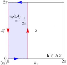
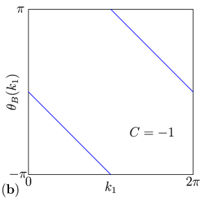
Figure 11: Landau Level Wilson Loops. $(a)$ The Berry phase can be calculated using Stokes’s theorem in Eq. (256). The red arrows represent Wilson loops integrated along $k_{2}$, and the blue arrows represent two additional paths (which sum to zero because $k_{2}=0$ and $k_{2}=2\pi$ are identified) which form a closed loop. There is an additional delta function marked by the X at $(k_{1},k_{2})=(\pi,\pi)$ which adds $2\pi$ to the Berry phase as $k_{1}$ crosses $\pi$. $(b)$ We plot the Berry phase obtained from the Abelian Wilson loop in Eq. (256), from which we see that the winding gives $C=-1$.

Having discussed the Abelian terms from the Landau level basis states, we now consider the full non-Abelian Wilson loop with contributions from the band eigenvectors. We gather the terms from Eq. (240) and Eq. (249). Incorporating the prefactors, we find

$$\braket{\mathbf{k}^{\prime},m}{\mathbf{b}_{i}\cdot\mathbf{r}}{\mathbf{k},n} =(2\pi)^{2}\delta_{mn}(-i\partial_{i})\delta(\mathbf{k}-\mathbf{k}^{\prime})$$ (257)

$$\qquad-(2\pi)^{2}\delta(\mathbf{k}-\mathbf{k}^{\prime})\epsilon_{ij}\Big{(}\frac{1}{2}\delta_{mn}\partial_{j}\log\mathcal{N}(\mathbf{k})+[\tilde{Z}_{j}]_{mn}\Big{)}\ .$$

The explicit matrix elements are

$$\hbox{}[\tilde{Z}_{j}]_{mn}=\braket{m}{\frac{z_{j}a^{\dagger}+\bar{z}_{j}a}{\sqrt{2\phi}}}{n}=\frac{1}{\sqrt{2\phi}}(z_{j}\sqrt{m}\delta_{m-1,n}+\bar{z}_{j}\sqrt{n}\delta_{m,n-1})\ .$$ (258)

Finally, we obtain an explicit expression for the non-Abelian Berry connection $\mathcal{A}^{MN}(\mathbf{k})$ in the occupied bands indexed by $M,N$ defined by

$$(2\pi)^{2}\delta(\mathbf{k}-\mathbf{k}^{\prime})\mathcal{A}^{MN}(\mathbf{k}) =\sum_{mn}[U^{\dagger}]^{M}_{m}\braket{\mathbf{k}^{\prime},m}{\mathbf{r}}{\mathbf{k},n}U_{n}^{N}(\mathbf{k})$$ (259)

where $U(\mathbf{k})$ is the $N_{LL}\times N_{occ}$ matrix of eigenvectors, $N_{occ}$ is the number of occupied bands, and $N_{LL}$ is the dimension of the matrix Hamiltonian after the Landau levels are truncated above some cutoff. Plugging in Eq. (249), we find the final expression

$$\boxed{\mathcal{A}_{i}^{MN}(\mathbf{k})={\bf{b}}_{i}\cdot\mathcal{A}^{MN}(\mathbf{k})=[U^{\dagger}(i\partial_{i}-\epsilon_{ij}\tilde{Z}_{j})U]^{MN}-\frac{\delta^{MN}}{2}\epsilon_{ij}\partial_{j}\log\vartheta\left(\left.\frac{(k_{1},k_{2})}{2\pi}\right|\Phi\right)}$$ (260)

where we performed an identical manipulation to Eq. (252) to act the $\partial_{i}$ derivative on $U(\mathbf{k})$.

To compute Wilson loops numerically, we need to be able to write the Wilson loop as a discretized product. To do so, we need to deal with the $\tilde{Z}_{j}$ term using the commutation relations in Eq. (228). We need the following identity

$$e^{-i\epsilon_{jl}k_{j}\tilde{Z}_{l}}\partial_{i}e^{i\epsilon_{jl}k_{j}\tilde{Z}_{l}} =i\epsilon_{il}\tilde{Z}_{l}-\frac{1}{2}[i\epsilon_{jl}k_{j}\tilde{Z}_{l},\partial_{i}(i\epsilon_{j^{\prime}l^{\prime}}k_{j^{\prime}}\tilde{Z}_{l^{\prime}})]+\text{higher commutators}$$ (261)

$$=i\epsilon_{il}\tilde{Z}_{l}+\frac{1}{2}\epsilon_{jl}\epsilon_{il^{\prime}}k_{j}[\tilde{Z}_{l},\tilde{Z}_{l^{\prime}}]$$

$$=i\epsilon_{ij}\tilde{Z}_{j}+\frac{i}{2\phi}\epsilon_{ll^{\prime}}\epsilon_{jl}\epsilon_{il^{\prime}}k_{j}$$

$$=i\epsilon_{ij}\tilde{Z}_{j}-\frac{i}{2\phi}\epsilon_{ij}k_{j}$$

where the first line is the formula for the derivative of the exponential map (see Wikipedia for instance https://en.wikipedia.org/wiki/Derivative_of_the_exponential_map) and the higher commutator terms vanish because $[\tilde{Z}_{i},\tilde{Z}_{j}]\propto\mathbb{1}$ is central. The additional $-\frac{i}{2\phi}\epsilon_{ij}k_{j}$ term has nonzero constant curl and so cannot be absorbed into the exponential. However, $-\frac{i}{2\phi}\epsilon_{ij}k_{j}$ is proportional to the identity so it can be factored out. Using Eq. (261), we have

$$U^{\dagger}(\mathbf{k})e^{-i\epsilon_{jl}k_{j}\tilde{Z}_{l}}i\partial_{i}\left(e^{i\epsilon_{jl}k_{j}\tilde{Z}_{l}}U(\mathbf{k})\right) =U^{\dagger}(\mathbf{k})\left(e^{-i\epsilon_{jl}k_{j}\tilde{Z}_{l}}i\partial_{i}e^{i\epsilon_{jl}k_{j}\tilde{Z}_{l}}\right)U(\mathbf{k})+U^{\dagger}(\mathbf{k})i\partial_{i}U(\mathbf{k})$$ (262)

$$=U^{\dagger}(\mathbf{k})i\partial_{i}U(\mathbf{k})+U^{\dagger}(\mathbf{k})\left(-\epsilon_{ij}\tilde{Z}_{j}+\frac{1}{2\phi}\epsilon_{ij}k_{j}\right)U(\mathbf{k})$$

$$=U^{\dagger}(\mathbf{k})\left(i\partial_{i}-\epsilon_{ij}\tilde{Z}_{j}\right)U(\mathbf{k})+\frac{1}{2\phi}\epsilon_{ij}k_{j}U^{\dagger}(\mathbf{k})U(\mathbf{k})$$

and because $U^{\dagger}(\mathbf{k})U(\mathbf{k})=\mathbb{1}$ due to the orthonormality of the eigenvectors, we arrive at

$$\mathcal{A}_{i}^{MN}(\mathbf{k}) =[\tilde{U}^{\dagger}i\partial_{i}\tilde{U}]^{MN}-\frac{\delta^{MN}}{2\phi}\epsilon_{ij}k_{j}-\frac{\delta^{MN}}{2}\epsilon_{ij}\partial_{j}\log\vartheta\left(\left.\frac{(k_{1},k_{2})}{2\pi}\right|\Phi\right),\qquad\tilde{U}(\mathbf{k})\equiv e^{i\epsilon_{ij}k_{i}{\tilde{Z}}_{j}}U(\mathbf{k})=\mathcal{H}^{\mathbf{k}}U(\mathbf{k})$$ (263)

and we used $e^{i\epsilon_{ij}k_{i}\tilde{Z}_{j}}=\mathcal{H}^{\mathbf{k}}$ which is a unitary matrix. As such, note that $\tilde{U}^{\dagger}(\mathbf{k})\tilde{U}(\mathbf{k})=U^{\dagger}(\mathbf{k}){\mathcal{H}^{\mathbf{k}}}^{\dagger}\mathcal{H}^{\mathbf{k}}U(\mathbf{k})=U^{\dagger}(\mathbf{k})U(\mathbf{k})=\mathbb{1}$. The exponential factor $e^{i\epsilon_{ij}k_{i}\tilde{Z}_{j}}$ has nontrivial commutation relations and cannot be absorbed into the definition of $U({\bf{k}})$ via a gauge transformation; we will keep this term throughout our calculations. The first term in Eq. (263) is in the canonical Berry connection form. The second term is the extraneous Abelian term (which we will show is canceled at the end of the calculation), and the third term of Eq. (263) is the winding of the Chern basis. As with the standard zero-flux Wilson loop, we want to express the Wilson loop as a product of projectors. In constructing the projector product, we will find that a term appears to exactly cancel the $-\frac{\delta^{MN}}{2\phi}\epsilon_{ij}k_{j}$ extraneous term. The end result will be a simple product formula in terms of $U(\mathbf{k})$. We define the path-ordered non-Abelian Wilson loop along the path $\mathcal{C}$ to be Alexandradinata:2012sp

$$\hbox{}[W_{\mathcal{C}}]^{MN} =\left[\exp\left(i\oint_{\mathcal{C}}d\mathbf{k}\cdot\mathcal{A}(\mathbf{k})\right)\right]^{MN}$$ (264)

We now plug in Eq. (263) and factor out the Abelian contributions:

$$W_{\mathcal{C}} =e^{-i\oint_{\mathcal{C}}d\mathbf{k}\times\frac{1}{2}\boldsymbol{\nabla}\log\vartheta\left(\left.\frac{(k_{1},k_{2})}{2\pi}\right|\Phi\right)}\left[e^{-\frac{i}{2\phi}\int_{\mathcal{C}}dk_{i}\epsilon_{ij}k_{j}}\exp\left(i\oint_{\mathcal{C}}dk_{i}\,\tilde{U}^{\dagger}i\partial_{i}\tilde{U}\right)\right]\ .$$ (265)

Note that we have grouped the extraneous Abelian term with the $\tilde{U}$ term inside the brackets. Our goal is now to produce a discretized expression for the bracketed term. To do so, we break the path $\mathcal{C}$ into $L$ increments labeled by $d\mathbf{k}_{n},n=1,\dots L$ where $d\mathbf{k}_{n}=\mathbf{k}_{n}-\mathbf{k}_{n-1}$. Because $\mathcal{C}$ is a closed path, $\mathbf{k}_{0}\equiv\mathbf{k}_{L}$. Taking $L\to\infty$, we find

$$\exp\left(i\oint_{\mathcal{C}}dk_{i}\,\tilde{U}^{\dagger}i\partial_{i}\tilde{U}\right) =\exp\left(i\sum_{n=1}^{L}\tilde{U}^{\dagger}(\mathbf{k}_{n})i(\tilde{U}(\mathbf{k}_{n})-\tilde{U}(\mathbf{k}_{n-1}))\right)$$ (266)

$$=\exp\left(i\sum_{n=1}^{L}i(\mathbb{1}-\tilde{U}^{\dagger}(\mathbf{k}_{n})\tilde{U}(\mathbf{k}_{n-1}))\right)$$

and now using BCH (neglecting terms of $O(d\mathbf{k}^{2})$ which vanish as $L\to\infty$), we have

$$\exp\left(i\oint_{\mathcal{C}}dk_{i}\,\tilde{U}^{\dagger}i\partial_{i}\tilde{U}\right) \to\prod_{n}^{L\leftarrow 1}\exp\left((-\mathbb{1}+\tilde{U}^{\dagger}(\mathbf{k}_{n})\tilde{U}(\mathbf{k}_{n-1}))\right)$$ (267)

$$=\prod_{n}^{L\leftarrow 1}\left(\mathbb{1}+(-\mathbb{1}+\tilde{U}^{\dagger}(\mathbf{k}_{n})\tilde{U}(\mathbf{k}_{n-1}))+\dots\right)$$

$$=\prod_{n}^{L\leftarrow 1}\tilde{U}^{\dagger}(\mathbf{k}_{n})\tilde{U}(\mathbf{k}_{n-1})$$

where in the second to last line, we expanded $e^{M}=1+M+\dots$ where $M=\tilde{U}^{\dagger}(\mathbf{k}_{n})\tilde{U}(\mathbf{k}_{n-1})-\mathbb{1}$ is a matrix of order $O(d\mathbf{k})$. Terms of higher order vanish in the $L\to\infty$ limit. So far, this argument is identical to the standard Wilson loop. Regrouping terms in the product gives the standard Wilson loop form

$$\exp\left(i\oint_{\mathcal{C}}dk_{i}\,\tilde{U}^{\dagger}i\partial_{i}\tilde{U}\right) =\tilde{U}^{\dagger}(\mathbf{k}_{L})\left(\prod_{n}^{L-1\leftarrow 1}\tilde{U}(\mathbf{k}_{n})\tilde{U}^{\dagger}(\mathbf{k}_{n})\right)\tilde{U}(\mathbf{k}_{0})\ .$$ (268)

The factors in parentheses are a product of $\tilde{U}$ projectors. By plugging in $\tilde{U}(\mathbf{k})=\mathcal{H}^{\mathbf{k}}U(\mathbf{k})$, we will arrive at an expression written only in terms of the matrix eigenvectors $U(\mathbf{k})$:

$$\prod_{n}^{L-1\leftarrow 1}\tilde{U}(\mathbf{k}_{n})\tilde{U}^{\dagger}(\mathbf{k}_{n}) =\mathcal{H}^{\mathbf{k}_{L-1}}P(\mathbf{k}_{L-1})\mathcal{H}^{-\mathbf{k}_{L-1}}\dots\mathcal{H}^{\mathbf{k}_{2}}P(\mathbf{k}_{2})\mathcal{H}^{-\mathbf{k}_{2}}\mathcal{H}^{\mathbf{k}_{1}}P(\mathbf{k}_{1})\mathcal{H}^{-\mathbf{k}_{1}},\quad P(\mathbf{k})\equiv U(\mathbf{k})U^{\dagger}(\mathbf{k})\ .$$ (269)

To simplify the Wilson loop further, we focus on factors in the form $\mathcal{H}^{-\mathbf{k}_{n+1}}\mathcal{H}^{\mathbf{k}_{n}}$. To do so, recall that $\mathcal{H}^{\mathbf{k}}=e^{i\epsilon_{ij}k_{i}\tilde{Z}_{j}}$ and use the Baker-Campbell-Hausdorff identity $e^{X+Y}=e^{-\frac{1}{2}[X,Y]}e^{X}e^{Y}$ for $[X,Y]$ a $c$-number to show

$$\mathcal{H}^{-\mathbf{k}_{n+1}}\mathcal{H}^{\mathbf{k}_{n}}=\mathcal{H}^{-d\mathbf{k}_{n+1}-\mathbf{k}_{n}}\mathcal{H}^{\mathbf{k}_{n}} =\exp\left(-\frac{1}{2}[-i\epsilon_{ij}dk^{n+1}_{i}\tilde{Z}_{j},-i\epsilon_{i^{\prime}j^{\prime}}k^{n}_{i^{\prime}}\tilde{Z}_{j^{\prime}}]\right)\mathcal{H}^{-d\mathbf{k}_{n+1}}\mathcal{H}^{-\mathbf{k}_{n}}\mathcal{H}^{\mathbf{k}_{n}}$$ (270)

where we raised the $n$ indices on $d\mathbf{k}$ and $\mathbf{k}$ to avoid confusion with the vector indices $i,j$. The commutator is direct to evaluate with Eq. (228):

$$\hbox{}[-i\epsilon_{ij}dk^{n+1}_{i}\tilde{Z}_{j},-i\epsilon_{i^{\prime}j^{\prime}}k^{n}_{i^{\prime}}\tilde{Z}_{j^{\prime}}] =-\epsilon_{ij}\epsilon_{i^{\prime}j^{\prime}}dk^{n+1}_{i}k^{n}_{i^{\prime}}[\tilde{Z}_{j},\tilde{Z}_{j^{\prime}}]$$ (271)

$$=-\epsilon_{ij}\epsilon_{i^{\prime}j^{\prime}}dk^{n+1}_{i}k^{n}_{i^{\prime}}\frac{i}{\phi}\epsilon_{jj^{\prime}}$$

$$=-\frac{i}{\phi}\epsilon_{ij}dk^{n+1}_{i}k^{n}_{j}$$

$$=-\frac{i}{\phi}d\mathbf{k}_{n+1}\times\mathbf{k}_{n}\ .$$

Returning to Eq. (270), we now have the simple relation

$$\mathcal{H}^{-\mathbf{k}_{n+1}}\mathcal{H}^{\mathbf{k}_{n}} =e^{\frac{i}{2\phi}d\mathbf{k}_{n+1}\times\mathbf{k}_{n}}\mathcal{H}^{-d\mathbf{k}_{n+1}}$$ (272)

using $\mathcal{H}^{-\mathbf{k}_{n}}\mathcal{H}^{\mathbf{k}_{n}}=\mathbb{1}$ by unitarity. With this result, Eq. (269) reads

$$\prod_{n}^{L-1\leftarrow 1}\tilde{U}(\mathbf{k}_{n})\tilde{U}^{\dagger}(\mathbf{k}_{n}) =e^{\frac{i}{2\phi}\sum_{n=1}^{L-2}d\mathbf{k}_{n+1}\times\mathbf{k}_{n}}\mathcal{H}^{\mathbf{k}_{L-1}}P(\mathbf{k}_{L-1})\dots\mathcal{H}^{-d\mathbf{k}_{3}}P(\mathbf{k}_{2})\mathcal{H}^{-d\mathbf{k}_{2}}P(\mathbf{k}_{1})\mathcal{H}^{-\mathbf{k}_{1}}$$ (273)

$$\tilde{U}^{\dagger}(\mathbf{k}_{L})\left(\prod_{n}^{L-1\leftarrow 1}\tilde{U}(\mathbf{k}_{n})\tilde{U}^{\dagger}(\mathbf{k}_{n})\right)\tilde{U}(\mathbf{k}_{n}) =e^{\frac{i}{2\phi}\sum_{n=0}^{L-1}d\mathbf{k}_{n+1}\times\mathbf{k}_{n}}U^{\dagger}(\mathbf{k}_{L})\mathcal{H}^{-d\mathbf{k}_{L}}P(\mathbf{k}_{L-1})\dots\mathcal{H}^{-d\mathbf{k}_{3}}P(\mathbf{k}_{2})\mathcal{H}^{-d\mathbf{k}_{2}}P(\mathbf{k}_{1})\mathcal{H}^{-d\mathbf{k}_{1}}U(\mathbf{k}_{0})$$

where we grouped the Abelian $-\frac{i}{\phi}d\mathbf{k}_{n+1}\times\mathbf{k}_{n}$ terms into an overall prefactor. Now we have a simple expression for the $\tilde{U}$ Wilson loop in Eq. (268) which reads

$$\exp\left(i\oint_{\mathcal{C}}dk_{i}\,\tilde{U}^{\dagger}i\partial_{i}\tilde{U}\right) =e^{\frac{i}{2\phi}\sum_{n=0}^{L-1}d\mathbf{k}_{n+1}\times\mathbf{k}_{n}}U^{\dagger}(\mathbf{k}_{L})\mathcal{H}^{-d\mathbf{k}_{L}}\left(\prod_{n}^{L-1\leftarrow 1}P(\mathbf{k}_{n})\mathcal{H}^{-d\mathbf{k}_{n}}\right)U(\mathbf{k}_{0})\ .$$ (274)

Because we have taken $L\to\infty$, the Abelian overall phase becomes

$$\lim_{L\to\infty}\frac{i}{2\phi}\sum_{n=0}^{L-1}d\mathbf{k}_{n+1}\times\mathbf{k}_{n}=\frac{i}{2\phi}\oint_{\mathcal{C}}dk_{i}\epsilon_{ij}k_{j}\ .$$ (275)

This prefactor exactly cancels the extraneous Abelian term in Eq. (265), which now reads

$$\boxed{W_{\mathcal{C}}=e^{-i\oint_{\mathcal{C}}d\mathbf{k}\times\frac{1}{2}\boldsymbol{\nabla}\log\vartheta(\frac{(k_{1},k_{2})}{2\pi}|\Phi)}U^{\dagger}(\mathbf{k}_{L})\mathcal{H}^{-d\mathbf{k}_{L}}P(\mathbf{k}_{L-1})\dots P(\mathbf{k}_{2})\mathcal{H}^{-d\mathbf{k}_{2}}P(\mathbf{k}_{1})\mathcal{H}^{-d\mathbf{k}_{1}}U(\mathbf{k}_{0})}$$ (276)

showing that the Wilson loop at $\phi=2\pi$ factors into an Abelian winding factor that gives each Landau level a nonzero Chern number, and a non-Abelian product of projectors with insertions of $\mathcal{H}^{-d\mathbf{k}}$. To understand the effect of the insertions, we consider the Berry connection (Eq. (260)) when all bands are occupied, so $U(\mathbf{k})=\mathbb{1}$. Because $U(\mathbf{k})$ is independent of $\mathbf{k}$ in this case, the $\mathbf{k}$ derivative term disappears and

$$\mathcal{A}_{i}^{MN}(\mathbf{k}) =[(-\epsilon_{ij}\tilde{Z}_{j})]^{MN}-\frac{\delta^{MN}}{2}\epsilon_{ij}\partial_{j}\log\vartheta\left(\left.\frac{(k_{1},k_{2})}{2\pi}\right|\Phi\right)\ .$$ (277)

In a crystal at zero flux, the Berry connection of fully occupied bands is identically zero, but we see from the above expression that two contributions survive at $\phi=2\pi$. Using Eq. (258) to show that $\tilde{Z}_{j}$ is traceless, we see that only the Abelian term (the second term in Eq. (277)) contributes to the Berry curvature and therefore the winding. However, the non-Abelian term is nontrivial. We compute the Wilson loop along a straight contour $\mathcal{C}=(k_{1},0)\to(k_{1},2\pi)$, finding:

$$W_{\mathcal{C}}=\exp\left(i\oint_{\mathcal{C}}dk_{i}\mathcal{A}_{i}(\mathbf{k})\right) =e^{i\oint_{\mathcal{C}}dk_{i}(-\epsilon_{ij}\tilde{Z}_{j})}e^{-i\oint_{\mathcal{C}}d\mathbf{k}\times\frac{1}{2}\boldsymbol{\nabla}\log\vartheta\left(\left.\frac{(k_{1},k_{2})}{2\pi}\right|\Phi\right)}$$ (278)

$$=e^{-i(2\pi\mathbf{b}_{2})_{i}\epsilon_{ij}\tilde{Z}_{j}}e^{-i\oint_{\mathcal{C}}d\mathbf{k}\times\frac{1}{2}\boldsymbol{\nabla}\log\vartheta\left(\left.\frac{(k_{1},k_{2})}{2\pi}\right|\Phi\right)}$$

$$=\mathcal{H}^{-2\pi\mathbf{b}_{2}}e^{-i\oint_{\mathcal{C}}d\mathbf{k}\times\frac{1}{2}\boldsymbol{\nabla}\log\vartheta\left(\left.\frac{(k_{1},k_{2})}{2\pi}\right|\Phi\right)}$$

showing that $\mathcal{H}^{-2\pi\mathbf{b}_{2}}$ can be interpreted as the non-Abelian factor of the Wilson loop in the fully occupied limit (note that it does not depend on $k_{1}$ so does not contribute to the winding). Importantly, this result agrees with Eq. (276) which in the $U(\mathbf{k})=\mathbb{1}$ limit reads

$$W_{\mathcal{C}} =e^{-i\oint_{\mathcal{C}}d\mathbf{k}\times\frac{1}{2}\boldsymbol{\nabla}\log\vartheta\left(\left.\frac{(k_{1},k_{2})}{2\pi}\right|\Phi\right)}\mathcal{H}^{-d\mathbf{k}_{L}}\left(\prod_{n}^{L-1\leftarrow 1}\mathcal{H}^{-d\mathbf{k}_{n}}\right)$$ (279)

$$=e^{-i\oint_{\mathcal{C}}d\mathbf{k}\times\frac{1}{2}\boldsymbol{\nabla}\log\vartheta\left(\left.\frac{(k_{1},k_{2})}{2\pi}\right|\Phi\right)}\prod_{n}^{L\leftarrow 1}\mathcal{H}^{-\frac{2\pi}{L}\mathbf{b}_{2}}$$

$$=e^{-i\oint_{\mathcal{C}}d\mathbf{k}\times\frac{1}{2}\boldsymbol{\nabla}\log\vartheta\left(\left.\frac{(k_{1},k_{2})}{2\pi}\right|\Phi\right)}\mathcal{H}^{-2\pi\mathbf{b}_{2}}$$

using Eq. (227) in the last line. The physical picture of Eq. (278) and Eq. (279) is that, unlike the atomic limits of zero-flux crystals, the fully occupied Landau level state has a nontrivial Wilson loop where every band winds identically due to the $\epsilon_{ij}\partial_{j}\log\vartheta$ term. The $k_{1}$-independent $\mathcal{H}^{-2\pi\mathbf{b}_{2}}$ term can be diagonalized to obtain the Wannier centers which are the Wilson loop eigenvalues Alexandradinata:2012sp; Marzari et al. (2012).

Appendix B Square Lattice Calculations

This section is brief, pedagogically oriented review of how Bloch’s theorem is used to produce a matrix Hamiltonian on a plane wave basis at zero flux (App. B.1) and how our magnetic Bloch theorem is used to produce a matrix Hamiltonian on a Landau level basis at $2\pi$ flux (App. B.2). We use a simple $p^{2}/(2m)$ kinetic Hamiltonian in a cosine potential on the square lattice.

B.1 Zero Flux

The zero-flux Hamiltonian is chosen to be

$$H^{\phi=0}({\bf{r}})=-\frac{1}{2}{\boldsymbol{\nabla}}^{2}+\frac{w}{2}(e^{-2\pi i{\bf{b}}_{1}\cdot{\bf{r}}}+e^{-2\pi i{\bf{b}}_{2}\cdot{\bf{r}}}+H.c.)$$ (280)

If $w=0$, the solution to the Hamiltonian is simple – the eigenstates are plane waves of the form

$$\tilde{\psi}_{\tilde{\bf{k}}}({\bf{r}})=e^{i{\tilde{\bf{k}}}\cdot{\bf{r}}},$$ (281)

where ${\tilde{\bf{k}}}$ runs over the entire plane $\mathbb{R}^{2}$. When the lattice potential is added, the continuous translation symmetry is broken down to a discrete symmetry indexed by ${\bf{k}}$, where ${\bf{k}}$ is defined in first Brillouin zone ${\bf{k}}=k_{1}{\bf{b}}_{1}+k_{2}{\bf{b}}_{2},k_{1,2}\in(-\pi,\pi]$ . States at $\mathbf{k}+2\pi\mathbf{G}$ where ${\bf{G}}=2\pi G_{1}{\bf{b}}_{1}+2\pi G_{2}{\bf{b}}_{2},G_{1,2}\in\mathbb{Z}$ can be scattered to states at $\mathbf{k}$ by the periodic potential. The states

$$\psi_{{\bf{k}},{\bf{G}}}({\bf{r}})=\tilde{\psi}_{{\bf{k}}-{\bf{G}}}({\bf{r}}).$$ (282)

form a basis of the Hilbert space on which we can find a representation of the Hamiltonian, which will necessarily be diagonal in $\mathbf{k}$. This selection rule arises because $\psi_{{\bf{k}},{\bf{G}}}({\bf{r}})$ is an eigenstate of the translation operator: $\psi_{{\bf{k}},{\bf{G}}}({\bf{r}}+\mathbf{a}_{i})=e^{i(\mathbf{k}+2\pi\mathbf{G})\cdot\mathbf{a}_{i}}\psi_{{\bf{k}},{\bf{G}}}({\bf{r}})=e^{i\mathbf{k}\cdot\mathbf{a}_{i}}\psi_{{\bf{k}},{\bf{G}}}({\bf{r}})$ using the fact that $\mathbf{G}\cdot\mathbf{a}_{i}\in\mathds{Z}$. For each crystal momentum ${\bf{k}}$ in the first BZ, the plane wave index ${\bf{G}}$ labels different states with the same crystal momentum.

We calculate the matrix elements of the Hamiltonian in the $\ket{{\bf{k}},{\bf{G}}}$ basis, where $\langle{\bf{r}}|{\bf{k}},{\bf{G}}\rangle=\psi_{{\bf{k}},{\bf{G}}}({\bf{r}})$. Working in the ${\bf{k}},{\bf{G}}$ basis, the Hamiltonian reads

$$\bra{{\bf{k}},{\bf{G}}}H^{\phi=0}\ket{{\bf{k}}^{\prime},{\bf{G}}^{\prime}} =\int d^{2}rd^{2}r^{\prime}\,\braket{{\bf{k}},{\bf{G}}}{{\bf{r}}}\bra{{\bf{r}}}H^{\phi=0}\ket{{\bf{r}}^{\prime}}\braket{{\bf{r}}^{\prime}}{{\bf{k}}^{\prime},{\bf{G}}^{\prime}}$$ (283)

$$=\int d^{2}rd^{2}r^{\prime}\,\psi^{*}_{{\bf{k}},{\bf{G}}}({\bf{r}})H^{\phi=0}({\bf{r}})\delta({\bf{r}}-{\bf{r}}^{\prime})\psi_{{\bf{k}}^{\prime},{\bf{G}}^{\prime}}({\bf{r}}^{\prime})$$

$$=\int d^{2}r\,e^{-i({\bf{k}}-{\bf{G}})\cdot{\bf{r}}}H^{\phi=0}({\bf{r}})e^{i({\bf{k}}^{\prime}-{\bf{G}}^{\prime})\cdot{\bf{r}}}$$

$$=\int d^{2}r\,e^{-i({\bf{k}}-{\bf{G}})\cdot{\bf{r}}}\left[\frac{1}{2}({\bf{k}}^{\prime}-{\bf{G}}^{\prime})^{2}+\frac{w}{2}(e^{-2\pi i{\bf{b}}_{1}\cdot{\bf{r}}}+e^{-2\pi i{\bf{b}}_{2}\cdot{\bf{r}}}+H.c.)\right]e^{i({\bf{k}}^{\prime}-{\bf{G}}^{\prime})\cdot{\bf{r}}}$$

The kinetic term has no position dependence, so

$$\int d^{2}r\,e^{-i({\bf{k}}-{\bf{G}})\cdot{\bf{r}}}\left[\frac{1}{2}({\bf{k}}^{\prime}-{\bf{G}}^{\prime})^{2}\right]e^{i({\bf{k}}^{\prime}-{\bf{G}}^{\prime})\cdot{\bf{r}}}=(2\pi)^{2}\delta(\mathbf{k}-\mathbf{k}^{\prime})\left[\frac{1}{2}({\bf{k}}^{\prime}-{\bf{G}}^{\prime})^{2}\delta_{\mathbf{G},\mathbf{G}^{\prime}}\right]$$ (284)

which is diagonal in $\mathbf{k}$ and $\mathbf{G}$. The potential term does have position dependence and will not be diagonal in $\mathbf{G}$:

$$\frac{w}{2}\int d^{2}r\,e^{-i({\bf{k}}-{\bf{G}})\cdot{\bf{r}}}\left[e^{-2\pi i{\bf{b}}_{1}\cdot{\bf{r}}}+e^{-2\pi i{\bf{b}}_{2}\cdot{\bf{r}}}+H.c.\right]e^{i({\bf{k}}^{\prime}-{\bf{G}}^{\prime})\cdot{\bf{r}}}$$ (285)

$$\qquad\qquad\qquad\qquad=\frac{w}{2}\int d^{2}r\,\left[e^{-i({\bf{k}}-{\bf{G}}-{\bf{k}}^{\prime}+{\bf{G}}^{\prime}-2\pi{\bf{b}}_{1})\cdot{\bf{r}}}+e^{-i({\bf{k}}-{\bf{G}}-{\bf{k}}^{\prime}+{\bf{G}}^{\prime}-2\pi{\bf{b}}_{2})\cdot{\bf{r}}}+H.c.\right]$$

$$\qquad\qquad\qquad\qquad=(2\pi)^{2}\delta(\mathbf{k}-\mathbf{k}^{\prime})\frac{w}{2}\left[\delta_{\mathbf{G}+2\pi\mathbf{b}_{1},\mathbf{G}^{\prime}}+\delta_{\mathbf{G}^{\prime}+2\pi\mathbf{b}_{1},\mathbf{G}}+\delta_{\mathbf{G}+2\pi\mathbf{b}_{2},\mathbf{G}}+\delta_{\mathbf{G}^{\prime}+2\pi\mathbf{b}_{2},\mathbf{G}}\right]\ .$$

This term is still diagonal in $\mathbf{k}$ as ensures by the translation symmetry. We derive the Bloch Hamiltonian

$$\bra{{\bf{k}},{\bf{G}}}H^{\phi=0}\ket{{\bf{k}}^{\prime},{\bf{G}}^{\prime}} =(2\pi)\delta(\mathbf{k}-\mathbf{k}^{\prime})H^{\phi=0}_{\mathbf{G},\mathbf{G}^{\prime}}(\mathbf{k}),$$ (286)

$$H^{\phi=0}_{\mathbf{G},\mathbf{G}^{\prime}}(\mathbf{k}) =\frac{1}{2}({\bf{k}}^{\prime}-{\bf{G}}^{\prime})^{2}\delta_{\mathbf{G},\mathbf{G}^{\prime}}+\frac{w}{2}(\delta_{\mathbf{G}+2\pi\mathbf{b}_{1},\mathbf{G}^{\prime}}+\delta_{\mathbf{G}^{\prime}+2\pi\mathbf{b}_{1},\mathbf{G}}+\delta_{\mathbf{G}+2\pi\mathbf{b}_{2},\mathbf{G}}+\delta_{\mathbf{G}^{\prime}+2\pi\mathbf{b}_{2},\mathbf{G}})\ .$$

The Bloch Hamiltonian can be thought of as an infinite matrix on the $\mathbf{G}$ basis as a function of $\mathbf{k}$. By imposing a cutoff on the $\mathbf{G}$ plane wave states, this matrix can be diagonalized and the spectrum obtained.

B.2 $2\pi$-flux

The Hamiltonian at $2\pi$ flux is created via canonical substitution, sending $-i\boldsymbol{\nabla}\rightarrow\boldsymbol{\pi}$:

$$H^{\phi=2\pi}({\bf{r}})=\frac{1}{2}{\boldsymbol{\pi}}^{2}+\frac{w}{2}(e^{-2\pi i{\bf{b}}_{1}\cdot{\bf{r}}}+e^{-2\pi i{\bf{b}}_{2}\cdot{\bf{r}}}+H.c.).$$ (287)

At $2\pi$ flux, the magnetic translation operators commute with $H^{\phi=2\pi}({\bf{r}})$ and allow us to represent $H^{\phi=2\pi}({\bf{r}})$ as a matrix acting on the $\ket{\mathbf{k},n}$ eigenstates of the magnetic translation operators. We see that the Landau levels play the role of the plane waves at zero flux. The substantial difference is that, instead of simple Bloch states, the magnetic translation eigenstates are given in Eq. (94).

The matrix elements in the magnetic translation basis read

$$\bra{{\bf{k}},m}H^{\phi=2\pi}({\bf{r}})\ket{{\bf{k}}^{\prime},n} =\bra{{\bf{k}},m}\phi(a^{\dagger}a+\frac{1}{2})+\frac{w}{2}(e^{-2\pi i{\bf{b}}_{1}\cdot{\bf{r}}}+e^{-2\pi i{\bf{b}}_{2}\cdot{\bf{r}}}+H.c.)\ket{{\bf{k}}^{\prime},n}$$ (288)

$$=(2\pi)^{2}\delta({\bf{k}}-{\bf{k}}^{\prime})\left[\phi(m+\frac{1}{2})\delta_{mn}+\frac{w}{2}(e^{-ik_{2}}\mathcal{H}^{2\pi\mathbf{b}_{1}}_{mn}+e^{ik_{1}}\mathcal{H}^{2\pi\mathbf{b}_{2}}_{mn}+H.c.)\right]$$

where we used $\frac{1}{2}{\boldsymbol{\pi}}^{2}=\phi(a^{\dagger}a+\frac{1}{2})$ which acts diagonal on the $m,n$ Landau level indices because $a^{\dagger}a\ket{n}=n\ket{n}$. The matrix elements of the potential term were computed in App. A.6, and an expression for $\mathcal{H}^{2\pi\mathbf{G}}$ may be found in Eq. (224). Thus the magnetic Bloch Hamiltonian $H^{\phi=2\pi}_{mn}({\bf{k}})$ is defined

$$\bra{{\bf{k}},m}H^{\phi=2\pi}({\bf{r}})\ket{{\bf{k}}^{\prime},n} =(2\pi)\delta(\mathbf{k}-\mathbf{k}^{\prime})H^{\phi=2\pi}_{mn}({\bf{k}})\ .$$ (289)

In analogy to the zero flux case, $H^{\phi=2\pi}_{mn}({\bf{k}})$ is a matrix on the $mn$ Landau level indices as a function of $\mathbf{k}$, and can be diagonalized by imposing a Landau level cutoff. See Fig. 12 for a comparison for the density of states obtained by our band structures versus the open momentum space method in Ref. Lian et al., 2021a.

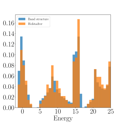
Figure 12: Density of states computed from the band structure (blue) versus the open momentum space method (orange) developed in Ref. Lian et al., 2021a. The small discrepancies can be improved by sampling more points in both methods.

Appendix C Coulomb Interaction in a Gauge-Invariant Formalism

In this Appendix, we show how to write the Coulomb interaction

$$H_{int} =\frac{1}{2}\int d^{2}rd^{2}r^{\prime}\,n(\mathbf{r})V(\mathbf{r}-\mathbf{r}^{\prime})n(\mathbf{r}^{\prime})=\frac{1}{2}\int\frac{d^{2}q}{(2\pi)^{2}}\,V(\mathbf{q})\rho_{-\mathbf{q}}\rho_{\mathbf{q}},$$ (290)

in the terms of the magnetic translation group eigenstates in a gauge-invariant manner. We keep $V(\mathbf{q})$ general but require the Fourier transform is even, $V(\mathbf{q})=V(-\mathbf{q})$, and is non-negative real, $V(\mathbf{q})\geq 0$, to preserve the positive semi-definite structure. We require a formula for the Fourier components of the density

$$\rho_{\mathbf{q}}=\int d^{2}r\,e^{-i\mathbf{q}\cdot\mathbf{r}}n(\mathbf{r})$$ (291)

written in terms of the magnetic translation group eigenstates. The single-particle magnetic translation group eigenstates are

$$\psi_{\mathbf{k},n}=\frac{1}{\sqrt{\mathcal{N}(\mathbf{k})}}\sum_{\mathbf{R}}e^{-i\mathbf{k}\cdot\mathbf{R}}T_{\mathbf{a}_{1}}^{\mathbf{R}\cdot\mathbf{b}_{1}}T_{\mathbf{a}_{2}}^{\mathbf{R}\cdot\mathbf{b}_{2}}\frac{a^{{\dagger}n}}{\sqrt{n!}}\psi_{0},\qquad a\psi_{0}=b\psi_{0}=0\ .$$ (292)

The single-particle eigenstates arises from diagonalizing the single-particle Hamiltonian on this basis, yielding matrix eigenvectors $U^{N}_{n}(\mathbf{k})$ where $N$ is the band index and $n$ is the Landau level orbital index. The continuum electron operators obey $\{c^{\dagger}(\mathbf{r}),c(\mathbf{r}^{\prime})\}=\delta(\mathbf{r}-\mathbf{r}^{\prime})$, and the creation operators for the magnetic translation group basis states are denoted $\gamma^{\dagger}_{\mathbf{k},N}=\sum_{n}U^{N}_{n}(\mathbf{k})\psi^{\dagger}_{\mathbf{k},n}$. The magnetic translation group eigenstates obey

$$\braket{\mathbf{r}}{\psi^{\dagger}_{\mathbf{k},n}}{0}=\braket{0}{c(\mathbf{r})\psi^{\dagger}_{\mathbf{k},n}}{0}=\psi_{\mathbf{k},n}(\mathbf{r})\ .$$ (293)

Our goal now is to express the density operator $n(\mathbf{r})=c^{\dagger}(\mathbf{r})c(\mathbf{r})$ in terms of the single-particle eigenstates. If there are any internal indices of $c$, like spin or valley in TBG, they are implicitly summed over: $n(\mathbf{r})=\sum_{\alpha}c_{\alpha}^{\dagger}(\mathbf{r})c_{\alpha}(\mathbf{r})$. Because $\rho(\mathbf{q})$ is bilinear in fermion operators, we only need to calculate its single-particle matrix elements. Inserting resolutions of the identity and using $\braket{\mathbf{r}^{\prime}}{n(\mathbf{r})}{\mathbf{r}^{\prime\prime}}=\delta(\mathbf{r}-\mathbf{r}^{\prime\prime})$, we find

$$\braket{0}{\psi_{\mathbf{k}^{\prime},m}\rho_{\mathbf{q}}\psi^{\dagger}_{\mathbf{k},n}}{0} =\int d^{2}r\,e^{-i{\bf{q}}\cdot{\bf{r}}}\braket{0}{\psi_{\mathbf{k}^{\prime},m}c^{\dagger}({\bf{r}})c({\bf{r}})\psi^{\dagger}_{\mathbf{k},n}}{0}$$ (294)

$$=\int d^{2}r\,e^{-i{\bf{q}}\cdot{\bf{r}}}\braket{0}{\psi_{\mathbf{k}^{\prime},m}c^{\dagger}({\bf{r}})}{0}\braket{0}{c({\bf{r}})\psi^{\dagger}_{\mathbf{k},n}}{0}$$

$$=\int d^{2}r\,e^{-i{\bf{q}}\cdot{\bf{r}}}\psi^{*}_{\mathbf{k}^{\prime},m}({\bf{r}})\psi_{\mathbf{k},n}({\bf{r}})$$

$$=\braket{\mathbf{k}^{\prime},m}{e^{-i\mathbf{q}\cdot\mathbf{r}}}{\mathbf{k},n}\ .$$

where in the second line we have inserted a resolution of identity, but because of fermion conservation only the vacuum survives. Hence we obtain an explicit expression for

$$\rho_{\mathbf{q}} =\sum_{mn}\int\frac{d^{2}kd^{2}k^{\prime}}{(2\pi)^{4}}\braket{\mathbf{k}^{\prime},m}{e^{-i\mathbf{q}\cdot\mathbf{r}}}{\mathbf{k},n}\psi^{\dagger}_{\mathbf{k}^{\prime},m}\psi_{\mathbf{k},n}$$ (295)

where the matrix element $\braket{\mathbf{k}^{\prime},m}{e^{-i\mathbf{q}\cdot\mathbf{r}}}{\mathbf{k},n}$ was computed in Eq. (236). This is essentially the density operator $\rho_{\bf{q}}$ in the Landau level basis. Thus we have determined the coefficients in the expansion of $\rho_{\mathbf{q}}$:

$$\rho_{\mathbf{q}} =\sum_{mn}\int\frac{d^{2}kd^{2}k^{\prime}}{(2\pi)^{4}}\braket{\mathbf{k}^{\prime},m}{e^{-i\mathbf{q}\cdot\mathbf{r}}}{\mathbf{k},n}\psi^{\dagger}_{\mathbf{k}^{\prime},m}\psi_{\mathbf{k},n}=\sum_{mn}\int\frac{d^{2}k}{(2\pi)^{2}}e^{i\xi_{\mathbf{q}}(\mathbf{k})}\psi^{\dagger}_{\mathbf{k}-\mathbf{q},m}\mathcal{H}^{\mathbf{q}}_{mn}\psi_{\mathbf{k},n}\ .$$ (296)

For convenience, we recall that

$$e^{i\xi_{\mathbf{q}}(\mathbf{k})} =\frac{e^{-\frac{\bar{q}q}{4\phi}}\vartheta\left(\left.\frac{(k_{1}-q/2,k_{2}+iq/2)}{2\pi}\right|\Phi\right)}{\sqrt{\vartheta\left(\left.\frac{(k_{1},k_{2})}{2\pi}\right|\Phi\right)\vartheta\left(\left.\frac{(k_{1}-q_{1},k_{2}-q_{2})}{2\pi}\right|\Phi\right)}}$$ (297)

$$\mathcal{H}^{\mathbf{q}}_{mn} =\bra{m}\exp\left(i\frac{\gamma_{q}a+\bar{\gamma}_{q}a^{\dagger}}{\sqrt{2\phi}}\right)\ket{n}=e^{-\frac{\bar{\gamma}_{q}\gamma_{q}}{4\phi}}\begin{cases}\sqrt{\frac{m!}{n!}}\left(\frac{i\gamma_{q}}{\sqrt{2\phi}}\right)^{n-m}L_{m}^{|n-m|}\left(\frac{\bar{\gamma}_{q}\gamma_{q}}{2\phi}\right),&n>m\\ \sqrt{\frac{n!}{m!}}\left(\frac{i\bar{\gamma}_{q}}{\sqrt{2\phi}}\right)^{m-n}L_{n}^{|m-n|}\left(\frac{\bar{\gamma}_{q}\gamma_{q}}{2\phi}\right),&m>n\\ \end{cases}$$

which are both unitary. It is simple now to write $\rho_{\mathbf{q}}$ in terms of the single-particle eigenstate basis by recalling that in the $N$th band

$$\gamma^{\dagger}_{\mathbf{k},N} =\sum_{m}U^{N}_{m}(\mathbf{k})\psi^{\dagger}_{\mathbf{k},m}\ .$$ (298)

The creation operator $\gamma_{{\bf{k}},N}^{\dagger}$ has no relation to the momentum factor $\gamma_{q}=\epsilon_{ij}q_{i}\bar{z}_{j}$. If our Landau levels carried additional indices $\alpha$, the unitary $U$ would also be a matrix in $\alpha,\beta$.

Orthogonality of the eigenvectors at a given $\mathbf{k}$ gives $\sum_{N}U^{N*}_{n}(\mathbf{k})\gamma^{\dagger}_{\mathbf{k},N}=\psi^{\dagger}_{\mathbf{k},n}$ and hence

$$\rho_{\mathbf{q}} =\int\frac{d^{2}k}{(2\pi)^{2}}e^{i\xi_{\mathbf{q}}(\mathbf{k})}\sum_{MN}\gamma^{\dagger}_{\mathbf{k}-\mathbf{q},M}[U^{\dagger}(\mathbf{k}-\mathbf{q})\mathcal{H}^{\mathbf{q}}U(\mathbf{k})]_{MN}\gamma_{\mathbf{k},N}\ .$$ (299)

To project the Hamiltonian into a set of low energy bands, one merely restricts the sum over $MN$. Our final step is to define the form factor

$$M_{MN}(\mathbf{k},\mathbf{q})\equiv e^{i\xi_{\mathbf{q}}(\mathbf{k})}[U^{\dagger}(\mathbf{k}-\mathbf{q})\mathcal{H}^{\mathbf{q}}U(\mathbf{k})]_{MN}\ .$$ (300)

A few comments about $M(\mathbf{k},\mathbf{q})$ are in order. For all $\mathbf{q}$, the eigenvalues of $M(\mathbf{k},\mathbf{q})$ have magnitudes less than or equal to $1$ because $e^{i\xi_{\mathbf{q}}(\mathbf{k})}\mathcal{H}^{\mathbf{q}}$ is unitary and $U(\mathbf{k})$ is composed from normalized eigenvectors. At generic $\mathbf{q}$, $M(\mathbf{k},\mathbf{q})$ does not have a gauge-invariant spectrum because $U(\mathbf{k})$ and $U(\mathbf{k}-\mathbf{q})$ are eigenvector matrices and each come with arbitrary phases. At $\mathbf{q}=2\pi\mathbf{G}$, $U(\mathbf{k})$ and $U(\mathbf{k}+2\pi\mathbf{G})$ are identical because $\mathbf{k}$ is periodic on the BZ. This is because the states $\psi_{\mathbf{k},n}(\mathbf{r})$ are explicitly periodic in $\mathbf{k}$, so Hamiltonian is explicitly translation-invariant. Thus $M(\mathbf{k},2\pi\mathbf{G})$ has a gauge-invariant spectrum. This eigenvector gauge-invariance is important because later expressions will depend on the spectrum of $M(\mathbf{k},2\pi\mathbf{G})$. Using $\mathcal{H}^{-\mathbf{q}}=\mathcal{H}^{\mathbf{q}\,{\dagger}}$, we find

$$M(\mathbf{k},\mathbf{q})^{\dagger}=e^{-i\xi_{\mathbf{q}}(\mathbf{k})}U^{\dagger}(\mathbf{k})\mathcal{H}^{-\mathbf{q}}U(\mathbf{k}-\mathbf{q})=e^{-i\xi_{\mathbf{q}}(\mathbf{k})-i\xi_{-\mathbf{q}}(\mathbf{k}-\mathbf{q})}M(\mathbf{k}-\mathbf{q},-\mathbf{q})=M(\mathbf{k}-\mathbf{q},-\mathbf{q})$$ (301)

where we used the theta function identity $e^{-i\xi_{\mathbf{q}}(\mathbf{k})-i\xi_{-\mathbf{q}}(\mathbf{k}-\mathbf{q})}=1$. This is proved by observing

$$e^{i\xi_{\mathbf{q}}(\mathbf{k})+i\xi_{-\mathbf{q}}(\mathbf{k}-\mathbf{q})} =\frac{e^{-\frac{\bar{q}q}{4\phi}}\vartheta\left(\left.\frac{(k_{1}-q/2,k_{2}+iq/2)}{2\pi}\right|\Phi\right)}{\sqrt{\vartheta\left(\left.\frac{(k_{1},k_{2})}{2\pi}\right|\Phi\right)\vartheta\left(\left.\frac{(k_{1}-q_{1},k_{2}-q_{2})}{2\pi}\right|\Phi\right)}}\frac{e^{-\frac{\bar{q}q}{4\phi}}\vartheta\left(\left.\frac{(k_{1}-q_{1}+q/2,k_{2}-q_{2}-iq/2)}{2\pi}\right|\Phi\right)}{\sqrt{\vartheta\left(\left.\frac{(k_{1}-q_{1},k_{2}-q_{2})}{2\pi}\right|\Phi\right)\vartheta\left(\left.\frac{(k_{1},k_{2})}{2\pi}\right|\Phi\right)}}$$ (302)

$$=e^{-\frac{\bar{q}q}{2\phi}}\frac{\vartheta\left(\left.\frac{(k_{1}-q/2,k_{2}+iq/2)}{2\pi}\right|\Phi\right)\vartheta\left(\left.\frac{(k_{1}-\bar{q}/2,k_{2}-i\bar{q}/2)}{2\pi}\right|\Phi\right)}{\vartheta\left(\left.\frac{(k_{1},k_{2})}{2\pi}\right|\Phi\right)\vartheta\left(\left.\frac{(k_{1}-q_{1},k_{2}-q_{2})}{2\pi}\right|\Phi\right)}$$

$$=e^{-\frac{\bar{q}q}{2\phi}}\frac{\left|\vartheta\left(\left.\frac{(k_{1}-q/2,k_{2}+iq/2)}{2\pi}\right|\Phi\right)\right|^{2}}{\vartheta\left(\left.\frac{(k_{1},k_{2})}{2\pi}\right|\Phi\right)\vartheta\left(\left.\frac{(k_{1}-q_{1},k_{2}-q_{2})}{2\pi}\right|\Phi\right)}>0$$

where we have used Eq. (118) which states $\theta(\mathbf{z}^{*}|\Phi)$ = $\theta(\mathbf{z}|\Phi)^{*}$ and that $\theta(\mathbf{z}|\Phi)$ is real and positive for $\mathbf{z}\in\mathbb{R}^{2}$. Because $|e^{i\xi_{\mathbf{q}}(\mathbf{k})+i\xi_{-\mathbf{q}}(\mathbf{k}-\mathbf{q})}|=1$ and $e^{i\xi_{\mathbf{q}}(\mathbf{k})+i\xi_{-\mathbf{q}}(\mathbf{k}-\mathbf{q})}$ is real and positive, we find $e^{i\xi_{\mathbf{q}}(\mathbf{k})+i\xi_{-\mathbf{q}}(\mathbf{k}-\mathbf{q})}=1$. Eq. (301) is the Hermiticity of form factor, as described in Ref. Bernevig et al., 2021c in zero flux where it is also true that $M^{\dagger}({\bf{k}},{\bf{q}})=M({\bf{k}}-{\bf{q}},-{\bf{q}})$.

Finally, we remark that $M(\mathbf{k}+2\pi\mathbf{G},\mathbf{q})=M(\mathbf{k},\mathbf{q})$ because $U(\mathbf{k}+2\pi\mathbf{G})=U(\mathbf{k})$ and $e^{i\xi_{\mathbf{q}}(\mathbf{k}+2\pi\mathbf{G})}=e^{i\xi_{\mathbf{q}}(\mathbf{k})}$ as follows from the periodicity of the Siegel theta functions in $\mathbf{k}$. However, $M(\mathbf{k},\mathbf{q})$ is not periodic in $\mathbf{q}$, which is expected because $\mathbf{q}\in\mathbb{R}^{2}$ is a continuum momentum. As a function of $\mathbf{q}$ at fixed $mn$, $\mathcal{H}^{\mathbf{q}}_{mn}$ is the product of a decaying exponential factor in $\gamma_{\mathbf{q}}\bar{\gamma}_{\mathbf{q}}\sim|\mathbf{q}|^{2}$ and a polynomial factor in $\gamma_{\mathbf{q}}$. Thus for large $\mathbf{q}$, this term will decay exponentially but with subleading power law growth.

We end this section with the explicit form of the Coulomb interaction Hamiltonian. The density operator is written in terms of the form factor via

$$\rho_{\mathbf{q}} =\int_{BZ}\frac{d^{2}k}{(2\pi)^{2}}\sum_{MN}M_{MN}(\mathbf{k},\mathbf{q})\gamma^{\dagger}_{\mathbf{k}-\mathbf{q},M}\gamma_{\mathbf{k},N}$$ (303)

which leads to the expression

$$H_{int}=\frac{1}{2}\int\frac{d^{2}q}{(2\pi)^{2}}\,V(\mathbf{q})\rho_{-\mathbf{q}}\rho_{\mathbf{q}} =\frac{1}{2}\int\frac{d^{2}q}{(2\pi)^{2}}\,O_{-\mathbf{q}}O_{\mathbf{q}},\qquad O_{\mathbf{q}}=\sqrt{V(\mathbf{q})}\int_{BZ}\frac{d^{2}k}{(2\pi)^{2}}\sum_{MN}M_{MN}(\mathbf{k},\mathbf{q})\gamma^{\dagger}_{\mathbf{k}-\mathbf{q},M}\gamma_{\mathbf{k},N}$$ (304)

which is positive semi-definite because $O_{-\mathbf{q}}=O_{\mathbf{q}}^{\dagger}$ as follows from Eq. (301). For numerical calculations, it is convenient to discretize the momentum integrals into a sum over $L^{2}$ terms according to

$$\int_{BZ}\frac{d^{2}k}{(2\pi)^{2}}f(\mathbf{k})\to\frac{1}{\Omega_{tot}}\sum_{\mathbf{k}\in BZ}f(\mathbf{k}),\qquad\int_{\mathbb{R}^{2}}\frac{d^{2}q}{(2\pi)^{2}}f(\mathbf{q})\to\frac{1}{\Omega_{tot}}\sum_{\mathbf{G}}\sum_{\mathbf{k}\in BZ}f(\mathbf{k}+2\pi\mathbf{G})$$ (305)

where $\Omega_{tot}=L^{2}\Omega$ is the total area of an $L\mathbf{a}_{1}\times L\mathbf{a}_{2}$ sample, and there are $L^{2}$ terms in the BZ sums, and the sum $\mathbf{G}$ is over the reciprocal lattice vectors $\mathbf{G}=\mathds{Z}\mathbf{b}_{1}+\mathds{Z}\mathbf{b}_{2}$. Notice that in Eq. (305), the ${\bf{k}}$ sum goes over the BZ. The $\mathbf{q}$ integral is over all of $\mathbb{R}^{2}$. It is useful to write $\mathbf{q}=\mathbf{k}+2\pi\mathbf{G}$ where $\mathbf{k}$ is integrated over the BZ and $\mathbf{G}$ is summed over the reciprocal lattice. Eq. (305) follows by approximating the $BZ$ integral as a sum.

Appendix D Bistritzer-MacDonald Hamiltonian at $2\pi$ Flux

In this Appendix, we discuss the Bistritzer-MacDonald (BM) model of TBG which is the central physical motivation for this work. In App. D.1, we lay out our conventions for the moiré unit cell, the Bistritzer-MacDonald (BM) Hamiltonian, and the explicit form of the single-particle Hamiltonian at $2\pi$ flux. We then discuss the symmetries of the full two-valley system which are relevant for the many-body calculations in App. D.2. A discussion of the strong coupling expansion used to treat the Coulomb interaction is given in App. D.3. App. D.4 contains a derivation of the exact eigenstates at even integer fillings.

D.1 Moiré Lattice Conventions and Single-particle Hamiltonian

Let us set our conventions for the geometry of the moiré twist unit cell. First, the graphene unit cell has a lattice vector of length $a_{g}=.246$nm and an area $\Omega_{g}=a_{g}^{2}\frac{\sqrt{3}}{2}$. The gaphene K point is $\mathbf{K}_{g}=\frac{2\pi}{a_{g}}(0,2/3)$. The moiré vectors are defined by the difference in momentum space of the rotated layers’ $K$ points:

$$2\pi\mathbf{q}_{1}=(R_{\theta/2}-R_{-\theta/2})\mathbf{K}_{g},\quad\mathbf{q}_{j}=C_{3}\mathbf{q}_{j-1},\quad 2\pi|\mathbf{q}_{j}|=k_{\theta}=2\sin\frac{\theta}{2}\,|\mathbf{K}_{g}|=\frac{8\pi\sin\frac{\theta}{2}}{3a_{g}}\ .$$ (306)

Note that in this convention, we keep a factor of $2\pi$ explicit. The moiré reciprocal lattice vectors are defined

$$\mathbf{b}_{j}=\mathbf{q}_{j}-\mathbf{q}_{3},\quad\mathbf{b}_{1}\times\mathbf{b}_{2} =\frac{(2\sin\frac{\theta}{2})^{2}}{\Omega_{g}},\qquad\mathbf{k}=k_{1}\mathbf{b}_{1}+k_{2}\mathbf{b}_{2},\ k_{i}\in(-\pi,\pi)\ .$$ (307)

Note that the moiré BZ has area $(2\pi)^{2}\mathbf{b}_{1}\times\mathbf{b}_{2}$ which is smaller than the graphene BZ by a factor of $(2\sin\frac{\theta}{2})^{2}\sim\theta^{2}$. This is because the lattice constant of the moiré unit cell is larger by a factor of $\theta$. The moire lattice is defined by $\mathbf{a}_{i}\cdot\mathbf{b}_{j}=\delta_{ij}$ which yields in cartesian coordinates

$$\mathbf{a}_{1}=\frac{a_{g}}{2\sin\frac{\theta}{2}}\left(-\frac{\sqrt{3}}{2},-\frac{1}{2}\right)\quad\mathbf{a}_{2}=\frac{a_{g}}{2\sin\frac{\theta}{2}}\left(\frac{\sqrt{3}}{2},-\frac{1}{2}\right),\qquad\Omega=\mathbf{a}_{1}\times\mathbf{a}_{2}=\frac{\Omega_{g}}{(2\sin\frac{\theta}{2})^{2}}\ .$$ (308)

In the range of the magic angle at $\theta=1.05^{\circ}$, the moiré unit cell is 3000 times larger than the graphene unit cell. The magnetic translation group is commutative when $\phi=\frac{eB\Omega}{\hbar}=2\pi$ where we temporarily restore $\hbar=h/(2\pi)$. In physical units, the corresponding magnetic field is in the range

$$B =\frac{h}{e\Omega}=\frac{h}{e\Omega_{g}}\theta^{2}\in(25,32)\text{T for }\theta\in(1.03^{\circ},1.15^{\circ})\ .$$ (309)

The BM Hamiltonian at $\phi=2\pi$ can be written (with $\sigma_{i}$ and $T_{j}$ acting on the sublattice indices)

$$H^{\phi}_{BM}(\mathbf{r}) =\begin{pmatrix}v_{F}\boldsymbol{\pi}\cdot\boldsymbol{\sigma}&T(\mathbf{r})^{\dagger}\\ T(\mathbf{r})&v_{F}\boldsymbol{\pi}\cdot\boldsymbol{\sigma}\\ \end{pmatrix},\qquad T(\mathbf{r})=\sum_{j=1}^{3}T_{j}e^{i2\pi\mathbf{q}_{j}\cdot\mathbf{r}},\quad T_{j+1}=\begin{pmatrix}w_{0}&w_{1}e^{-\frac{2\pi i}{3}j}\\ w_{1}e^{\frac{2\pi i}{3}j}&w_{0}\\ \end{pmatrix}\ .$$ (310)

In this gauge, Hamiltonian is not in Bloch form because the off-diagonals are do not have the lattice periodicity. This is because of the offset of the layer BZs. To remedy this, we perform a unitary transformation with the momentum shift matrix $\text{diag}(e^{i\pi\mathbf{q}_{1}\cdot\mathbf{r}},e^{-i\pi\mathbf{q}_{1}\cdot\mathbf{r}})$ which puts the Hamiltonian in Bloch form

$$H^{\phi}(\mathbf{r}) =\begin{pmatrix}v_{F}\boldsymbol{\pi}\cdot\boldsymbol{\sigma}-\pi v_{F}\mathbf{q}_{1}\cdot\boldsymbol{\sigma}&T_{1}+T_{2}e^{-i2\pi\mathbf{b}_{1}\cdot\mathbf{r}}+T_{3}e^{-i2\pi\mathbf{b}_{2}\cdot\mathbf{r}}\\ T_{1}+T_{2}e^{i2\pi\mathbf{b}_{1}\cdot\mathbf{r}}+T_{3}e^{i2\pi\mathbf{b}_{2}\cdot\mathbf{r}}&v_{F}\boldsymbol{\pi}\cdot\boldsymbol{\sigma}+\pi v_{F}\mathbf{q}_{1}\cdot\boldsymbol{\sigma}\\ \end{pmatrix},\qquad\mathbf{b}_{j}=\mathbf{q}_{j+1}-\mathbf{q}_{1}\ .$$ (311)

We now need to compute the overlaps of this matrix with the magnetic Bloch irrep states. A suitable basis is $\ket{\mathbf{k},l,\alpha,n}\equiv\ket{l}\otimes\ket{\alpha}\otimes\ket{\mathbf{k},n}$ where $l=0,1$ is the layer index and $\alpha=0,1$ is the sublattice index. The Hamiltonian in this basis reads

$$H^{\phi=2\pi}(\mathbf{k})=\begin{pmatrix}v_{F}k_{\theta}(\sqrt{\frac{\phi}{2\pi}}h(\boldsymbol{\pi})-\frac{1}{2}\sigma_{2})&T_{1}+T_{2}e^{-ik_{2}}\mathcal{H}^{2\pi\mathbf{b}_{1}}+T_{3}e^{ik_{1}}\mathcal{H}^{2\pi\mathbf{b}_{2}}\\ T_{1}+T_{2}e^{ik_{2}}\mathcal{H}^{-2\pi\mathbf{b}_{1}}+T_{3}e^{-ik_{1}}\mathcal{H}^{-2\pi\mathbf{b}_{2}}&v_{F}k_{\theta}(\sqrt{\frac{\phi}{2\pi}}h(\boldsymbol{\pi})+\frac{1}{2}\sigma_{2})\end{pmatrix},\quad h(\boldsymbol{\pi})=\left(\frac{3\sqrt{3}}{2\pi}\right)^{1/2}\begin{pmatrix}0&a^{\dagger}\\ a&0\\ \end{pmatrix}$$ (312)

where $a,a^{\dagger},\mathcal{H}^{2\pi\mathbf{b}_{1}}$ are all matrices in the Landau level basis. We compute the band structure of this matrix by truncating the Landau levels from $n=0,\dots,n_{LL}$. Because of the truncation, the highest Landau level will be annihilated by the kinetic term, and introduces a two spurious states at each $\mathbf{k}$ (one per layer). These bands are easily removed.

D.2 Symmetries

In this section, we discuss the single-particle BM Hamiltonians in the $K$ and $K^{\prime}$ valleys and demonstrate the $U(1)$ valley symmetry, $C_{2z}$, and $P$ symmetries which survive at all flux and are essential for the Coulomb Hamiltonian in App. D.3. We also discuss the chiral symmetry $C$.

The BM Hamiltonian at zero flux reads

$$H_{K}^{\phi=0}=\begin{pmatrix}-iv_{F}\boldsymbol{\nabla}\cdot\boldsymbol{\sigma}&T({\bf{r}})^{\dagger}\\ T({\bf{r}})&-iv_{F}\boldsymbol{\nabla}\cdot\boldsymbol{\sigma}\end{pmatrix},$$ (313)

where the $T(\mathbf{r})$ moiré potentials are given in Eq. (310). In particular, $T_{1}=w_{0}\sigma_{0}+w_{1}\sigma_{1}$ and $T_{j}=e^{\frac{2\pi i(j-1)}{3}\sigma_{3}}T_{1}e^{-\frac{2\pi i(j-1)}{3}\sigma_{3}}$. The matrices $\sigma_{i}$ are Pauli matrices acting on the graphene sublattice index. The layer index is often in matrix notation, as in Eq. (313), and we will use $\tau_{i}$ Pauli matrices to denote the layer index as well. For many-body calculations, we must also study the Hamiltonian in the $K^{\prime}$ valley, which is related to the $K$ valley Hamiltonian at $\phi=0$ by spinless time reversal $T$ which acts as complex conjugation:

$$H_{K^{\prime}}^{\phi=0}=\begin{pmatrix}iv_{F}\boldsymbol{\nabla}\cdot\boldsymbol{\sigma}^{*}&T^{*}({\bf{r}})^{\dagger}\\ T^{*}({\bf{r}})&iv_{F}\boldsymbol{\nabla}\cdot\boldsymbol{\sigma}^{*}\end{pmatrix}\ .$$ (314)

The two Hamiltonians in Eq. (313) and Eq. (314) can be written as

$$H^{\phi=0}_{K} =-iv_{F}\tau_{0}(\sigma_{1}\partial_{x}+\sigma_{2}\partial_{y})+\sum_{j=1}^{3}\tau_{1}\cos(2\pi{\bf{q}}_{j}\cdot{\bf{r}})T_{j}+\tau_{2}\sin(2\pi{\bf{q}}_{j}\cdot{\bf{r}})T_{j}$$ (315)

$$H^{\phi=0}_{K^{\prime}} =iv_{F}\tau_{0}(\sigma_{1}\partial_{x}-\sigma_{2}\partial_{y})+\sum_{j=1}^{3}\tau_{1}\cos(2\pi{\bf{q}}_{j}\cdot{\bf{r}})T_{j}^{*}-\tau_{2}\sin(2\pi{\bf{q}}_{j}\cdot{\bf{r}})T_{j}^{*}.$$

We will use $\mu_{i}$ as the Pauli matrices acting on the graphene valley degree of freedom while $\tau_{i}$ are the Pauli matrices acting on the layer. In this notation, Eq. (315) can be written as one equation:

$$H^{\phi=0}(\mathbf{r}) =-iv_{F}\tau_{0}(\mu_{3}\sigma_{1}\partial_{x}+\mu_{0}\sigma_{2}\partial_{y})+\sum_{j=1}^{3}(\mu_{0}\tau_{1}\cos 2\pi{\bf{q}}_{j}\cdot{\bf{r}}+\mu_{3}\tau_{2}\sin 2\pi{\bf{q}}_{j}\cdot{\bf{r}})e^{\frac{2\pi i}{3}(j-1)\mu_{3}\sigma_{3}}T_{1}e^{-\frac{2\pi i}{3}(j-1)\mu_{3}\sigma_{3}}$$ (316)

which is the full two-valley Hamiltonian. It is direct to check that time reversal is a symmetry of $H^{\phi=0}$ (which it must be because $H^{\phi=0}$ is simply the $K$ valley with its time-reversed partner) by using the form $\mathcal{T}=\mu_{1}K,\mathcal{T}^{2}=+1$ on the two-valley model:

$$\mathcal{T}H^{\phi=0}(\mathbf{r})\mathcal{T}^{-1} =\mu_{1}\left(iv_{F}\tau_{0}(\mu_{3}\sigma_{1}\partial_{x}-\mu_{0}\sigma_{2}\partial_{y})+\sum_{j=1}^{3}(\mu_{0}\tau_{1}\cos 2\pi{\bf{q}}_{j}\cdot{\bf{r}}-\mu_{3}\tau_{2}\sin 2\pi{\bf{q}}_{j}\cdot{\bf{r}})e^{-\frac{2\pi i}{3}(j-1)\mu_{3}\sigma_{3}}T_{1}e^{\frac{2\pi i}{3}(j-1)\mu_{3}\sigma_{3}}\right)\mu_{1}$$ (317)

$$=iv_{F}\tau_{0}(-\mu_{3}\sigma_{1}\partial_{x}-\mu_{0}\sigma_{2}\partial_{y})+\sum_{j=1}^{3}(\mu_{0}\tau_{1}\cos 2\pi{\bf{q}}_{j}\cdot{\bf{r}}+\mu_{3}\tau_{2}\sin 2\pi{\bf{q}}_{j}\cdot{\bf{r}})e^{(-1)^{2}\frac{2\pi i}{3}(j-1)\mu_{3}\sigma_{3}}T_{1}e^{-\frac{2\pi i}{3}(j-1)\mu_{3}\sigma_{3}}$$

$$=H^{\phi=0}(\mathbf{r})\ .$$

It is now a simple matter to obtain the real space Hamiltonian at nonzero flux with the canonical substitution $-i\boldsymbol{\nabla}\to\boldsymbol{\pi}$ yielding

$$H^{\phi}(\mathbf{r}) =v_{F}\tau_{0}(\mu_{3}\sigma_{1}\pi_{x}+\mu_{0}\sigma_{2}\pi_{y})+\sum_{j=1}^{3}(\mu_{0}\tau_{1}\cos 2\pi{\bf{q}}_{j}\cdot{\bf{r}}+\mu_{3}\tau_{2}\sin 2\pi{\bf{q}}_{j}\cdot{\bf{r}})e^{\frac{2\pi i}{3}(j-1)\mu_{3}\sigma_{3}}T_{1}e^{-\frac{2\pi i}{3}(j-1)\mu_{3}\sigma_{3}}$$ (318)

Eq. 318 is the central result of this section, making it a simple matter to determine the symmetries of the model at all flux, and then transform them into a momentum or Landau level basis. It is direct to check that

$$\mathcal{T}H^{\phi}(\mathbf{r})\mathcal{T}^{-1}=H^{-\phi}(\mathbf{r})$$ (319)

because $\mathcal{T}(-i\boldsymbol{\nabla}+e\mathbf{A}(\mathbf{r}))\mathcal{T}^{-1}=i\boldsymbol{\nabla}+e\mathbf{A}(\mathbf{r})$, so $-i\boldsymbol{\nabla}$ and $\mathbf{A}$ do not transform the same way unless the magnetic field is flipped. This is expected because a magnetic field is known to break time reversal.

The first and most important symmetry is $U(1)$ valley which is a continuous symmetry generated by $\mu_{3}$ (note that $\mu_{1}$ and $\mu_{2}$ do not appear in Eq. (318) because the valleys are decoupled) which remains at all flux. There are three discrete symmetries of interest to us: inversion $C_{2z}$, unitary particle-hole $P$, and chiral symmetry $C$ when $w_{0}=0$. All three survive in nonzero flux. The actions of these symmetries on the full two-valley Hamiltonian are

$$C_{2z}H^{\phi}(\mathbf{r})C_{2z}^{\dagger} =H^{\phi}(\mathbf{r}),\qquad C_{2z}^{2}=+1$$ (320)

$$PH^{\phi}(\mathbf{r})P^{\dagger} =-H^{\phi}(\mathbf{r}),\qquad P^{2}=-1$$

$$CH^{\phi}(\mathbf{r})C =-H^{\phi}(\mathbf{r}),\qquad C^{2}=+1,\qquad\text{when $w_{0}=0$}\ .$$

We now derive the forms of these symmetries in real space for all flux, momentum space at zero flux, and on the Landau level basis of the magnetic Bloch Hamiltonian at $2\pi$ flux.

D.2.1 Real Space, all flux

We begin by proving the real-space form of the symmetries which can be derived from first principles in the continuum model. The results of this section alone are sufficient to check the physical symmetries of the BM model in flux. In App. D.2.2, we check that the same symmetries can also be written in momentum space, matching the expressions derived in Ref. Song et al. (2019).

To start, we analyze the $C_{2z}$ which acts as a $\pi$ rotation around the center of the graphene honeycomb unit cell. Hence, it takes $\mathbf{r}\to-\mathbf{r}$ (switching the sublattice index) and hence inverts the momentum (switching the graphene valley). $C_{2z}$ performs a rotation around the vector normal to the plane, and thus it does not act on the layer index. From this geometry, we arrive at

$$C_{2z} =\sigma_{1}\mu_{1}e^{i\pi L_{z}}$$ (321)

where $L_{z}$ is the angular momentum operator given by

$$L_{z}=\frac{\boldsymbol{\pi}^{2}-\mathbf{Q}^{2}}{2eB}=-i\epsilon_{\mu\nu}x_{\mu}\partial_{\nu}$$ (322)

where in the second equality we used the symmetric gauge. By working in the symmetric gauge, one can see explicitly that the $L_{z}$ operator is the same as at zero flux. However, we prefer to use the gauge-invariant $L_{z}$ operator for the sake of generality. In this case it is easy to show in any gauge that the gauge-invariant inversion operator $e^{i\pi L_{z}}$ reverses the canonical momentum

$$e^{i\pi L_{z}}\boldsymbol{\pi}e^{-i\pi L_{z}}=-\boldsymbol{\pi}\ .$$ (323)

We check directly that $D[C_{2z}]$ is a symmetry by computing

$$C_{2z}H^{\phi}(\mathbf{r})C_{2z}^{\dagger} =\sigma_{1}\mu_{1}\left(-v_{F}\tau_{0}(\mu_{3}\sigma_{1}\pi_{x}+\mu_{0}\sigma_{2}\pi_{y})+\sum_{j=1}^{3}(\mu_{0}\tau_{1}\cos 2\pi{\bf{q}}_{j}\cdot{\bf{r}}-\mu_{3}\tau_{2}\sin 2\pi{\bf{q}}_{j}\cdot{\bf{r}})e^{\frac{2\pi i}{3}(j-1)\mu_{3}\sigma_{3}}T_{1}e^{-\frac{2\pi i}{3}(j-1)\mu_{3}\sigma_{3}}\right)\sigma_{1}\mu_{1}$$ (324)

$$=-v_{F}\tau_{0}(-\mu_{3}\sigma_{1}\partial_{x}-\mu_{0}\sigma_{2}\partial_{y})+\sum_{j=1}^{3}(\mu_{0}\tau_{1}\cos 2\pi{\bf{q}}_{j}\cdot{\bf{r}}+\mu_{3}\tau_{2}\sin 2\pi{\bf{q}}_{j}\cdot{\bf{r}})e^{(-1)^{2}\frac{2\pi i}{3}(j-1)\mu_{3}\sigma_{3}}T_{1}e^{-(-1)^{2}\frac{2\pi i}{3}(j-1)\mu_{3}\sigma_{3}}$$

$$=H^{\phi}(\mathbf{r})$$

which is the correct behavior for the two-valley Hamiltonian. We now discuss the unitary particle-hole symmetry $P$ which acts as inversion in real space and also interchanges the layers, so it takes the form

$$P =i\tau_{2}\mu_{3}e^{i\pi L_{z}}\ .$$ (325)

The factor of $i$ ensures $P$ is real and commutes with $\mathcal{T}$. We check the action of $P$ directly:

$$PH^{\phi}(\mathbf{r})P^{\dagger} =\tau_{2}\mu_{3}\left(-v_{F}\tau_{0}(\mu_{3}\sigma_{1}\pi_{x}+\mu_{0}\sigma_{2}\pi_{y})+\sum_{j=1}^{3}(\mu_{0}\tau_{1}\cos 2\pi{\bf{q}}_{j}\cdot{\bf{r}}-\mu_{3}\tau_{2}\sin 2\pi{\bf{q}}_{j}\cdot{\bf{r}})e^{\frac{2\pi i}{3}(j-1)\mu_{3}\sigma_{3}}T_{1}e^{-\frac{2\pi i}{3}(j-1)\mu_{3}\sigma_{3}}\right)\tau_{2}\mu_{3}$$ (326)

$$=-v_{F}\tau_{0}(\mu_{3}\sigma_{1}\pi_{x}+\mu_{0}\sigma_{2}\pi_{y})+\sum_{j=1}^{3}(-\mu_{0}\tau_{1}\cos 2\pi{\bf{q}}_{j}\cdot{\bf{r}}-\mu_{3}\tau_{2}\sin 2\pi{\bf{q}}_{j}\cdot{\bf{r}})e^{\frac{2\pi i}{3}(j-1)\mu_{3}\sigma_{3}}T_{1}e^{-\frac{2\pi i}{3}(j-1)\mu_{3}\sigma_{3}}$$

$$=-H^{\phi}(\mathbf{r})\ .$$

An identical calculation shows that $P^{\prime}=i\tau_{2}\mu_{0}e^{i\pi L_{z}}$ (and thus any diagonal $\mu$ matrix) also anti-commutes with $H^{\phi}(\mathbf{r})$, which shows that $P$ is not only an anti-commuting symmetry of the two-valley model, but also of each valley individually. This is due to the $U(1)$ valley symmetry. Lastly, it is trivial to show that the chiral symmetry

$$C=\tau_{0}\sigma_{3}\mu_{0}$$ (327)

anti-commutes with $H^{\phi}(\mathbf{r})$ when $w_{0}=0$ (the first chiral limit) because

$$\sigma_{3}e^{\frac{2\pi i}{3}(j-1)\mu_{3}\sigma_{3}}T_{1}e^{-\frac{2\pi i}{3}(j-1)\mu_{3}\sigma_{3}}\sigma_{3} =w_{1}e^{\frac{2\pi i}{3}(j-1)\mu_{3}\sigma_{3}}\sigma_{3}\sigma_{1}\sigma_{3}e^{-\frac{2\pi i}{3}(j-1)\mu_{3}\sigma_{3}}$$ (328)

$$=-w_{1}e^{\frac{2\pi i}{3}(j-1)\mu_{3}\sigma_{3}}\sigma_{1}e^{-\frac{2\pi i}{3}(j-1)\mu_{3}\sigma_{3}}$$

and $\sigma_{3}$ trivially anti-commutes with the kinetic term because it only contains $\sigma_{1}$ and $\sigma_{2}$ matrices. Note that $\tau_{0}\sigma_{3}\mu_{3}$ also anti-commutes with $H^{\phi}(\mathbf{r})$, so $C$ is an anti-commuting symmetry of both valleys individually.

Our calculations establish that $C_{2z}$, $P$, and the chiral symmetry $C$ at $w_{0}=0$ are unbroken by flux. Because $\mathcal{T}$ reverses the flux, $C_{2z}\mathcal{T}$ is not a symmetry at $\phi\neq 0$, which has a significant effect on the topology. Finally, it is direct to check that $\{P,C_{2z}\}=0$ arising from the anti-commutation of the valley factors $\mu_{1}$ and $\mu_{3}$ and hence $(C_{2z}P)^{2}=-P^{2}C_{2z}^{2}=+1$. The most important observation is that $C_{2z}P=\mu_{2}\tau_{2}\sigma_{1}$ which is local in real space: the $e^{i\pi L_{z}}$ operators have canceled.

D.2.2 Zero flux, Momentum space

Although it is not required for this work, we now connect the real space symmetry operators we have derived in App. D.2.1 to the momentum space symmetries familiar in zero flux. We will follow heavily Ref. Bernevig et al., 2021c.

First, let us ignore interlayer coupling in the BM model. The two sheets of graphene have four Dirac cones (two for layer and two for spin.) If the standard sheet of graphene has Dirac cones at $\tilde{{\bf{k}}}={\bf{K}}_{g},-{\bf{K}}_{g}$, then in twisted bilayer graphene they occur at ${\bf{K}}_{+}=M_{\theta/2}{\bf{K}}_{g},-{\bf{K}}_{+}=-M_{\theta/2}{\bf{K}}_{g},$ for the top layer, and ${\bf{K}}_{-}=M_{-\theta/2}{\bf{K}}_{g},-{\bf{K}}_{-}=-M_{-\theta/2}{\bf{K}}_{g}$ for the bottom. Here $M_{\pm\theta/2}$ is a rotation matrix. Adding interlayer coupling reduces the graphene translation symmetry to the (approximate) moiré translation symmetry; momenta separated by reciprocal lattice vectors ${\bf{Q}}=2\pi m{\bf{b}}_{1}+2\pi n{\bf{b}}_{2}$ become identified. In the folded moiré BZ, the four Dirac cones are located at the moiré $K$ points ${\bf{K}}_{M}=\pi{\bf{q}}_{1},-{\bf{K}}_{M}=-\pi{\bf{q}}_{1}$ which each host $2$ Dirac cones (one per valley). Define the two ${\cal Q}$ sublattices to be

$${\cal Q}_{+} =\{\pi{\bf{q}}_{1}+2\pi m{\bf{b}}_{1}+2\pi n{\bf{b}}_{2}|m,n\in\mathbb{Z}\}$$ (329)

$${\cal Q}_{-} =\{-\pi{\bf{q}}_{1}+2\pi m{\bf{b}}_{1}+2\pi n{\bf{b}}_{2}|m,n\in\mathbb{Z}\}.$$ (330)

The two Dirac points ${\bf{K}}_{+},-{\bf{K}}_{-}\in{\cal Q}_{+}$, while ${\bf{K}}_{-},-{\bf{K}}_{+}\in{\cal Q}_{-}$. Thus, if we define

$$\zeta_{\bf{Q}}=\begin{cases}+1,~{}~{}{\bf{Q}}\in{\cal Q}_{+}\\ -1,~{}~{}{\bf{Q}}\in{\cal Q}_{-},\end{cases}$$ (331)

then $\zeta_{\bf{Q}}=\eta l$, with $\eta$ as the valley and $l$ the layer. We are now in a position to define the Fourier-transformed states.

$$c^{\dagger}_{{\bf{k}},{\bf{Q}},\eta,\alpha,s}=\frac{1}{\sqrt{N}}\sum_{\tilde{{\bf{R}}}\text{ in layer }l}e^{i({\bf{k}}+\eta{\bf{K}}_{l}-{\bf{Q}})\cdot(\tilde{{\bf{R}}}+\boldsymbol{t}_{\alpha})}c_{\tilde{{\bf{R}}},l,\alpha,s}^{\dagger},\qquad\text{with $\mathbf{Q},\eta,$ and $l$ obeying }\ l=\zeta_{\bf{Q}}\eta,$$ (332)

where $\boldsymbol{t}_{\alpha}$ is the graphene sublattice vector, $\alpha$ is the sublattice index, $l=\pm$ is the layer, $\tilde{\mathbf{R}}$ is the graphene Bravais lattice, and $s$ is the spin. The decoupled valleys are indexed by $\eta=\pm$.

We now study the matrix form of the symmetry operators. Define the unitary component of the symmetry $g$ as $D(g)$, where

$$gc_{{\bf{k}},{\bf{Q}},\eta,\alpha,s}^{\dagger}g^{-1}=c_{g{\bf{k}},{\bf{Q}}^{\prime},\eta^{\prime},\alpha^{\prime},s^{\prime}}^{\dagger}[D(g)]_{{\bf{Q}},\eta,\alpha,s,{\bf{Q}}^{\prime},\eta^{\prime},\alpha^{\prime},s^{\prime}}\ .$$ (333)

Applying $T$ to Eq. (332) gives

$${\cal T}c^{\dagger}_{{\bf{k}},{\bf{Q}},\eta,\alpha,s}{\cal T}^{-1}=\frac{1}{\sqrt{N}}\sum_{\tilde{{\bf{R}}}\text{ in layer }l}e^{-i({\bf{k}}+\eta{\bf{K}}_{l}-{\bf{Q}})\cdot(\tilde{{\bf{R}}}+\boldsymbol{t}_{\alpha})}{\cal T}c_{\tilde{{\bf{R}}},l,\alpha,s}^{\dagger}{\cal T}^{-1}$$ (334)

$$=c^{\dagger}_{-{\bf{k}},-{\bf{Q}},-\eta,\alpha,s}$$ (335)

so $D[{\cal T}]=\delta_{{\bf{Q}},-{\bf{Q}}^{\prime}}\mu_{1}$ and $\mathcal{T}$ takes ${\bf{k}}\rightarrow-{\bf{k}}$. Because both $\zeta_{\bf{Q}}$ and $\eta$ change, the layer remains the same. This matches the real-space picture because $\mathcal{T}$ is local.

A similar calculation holds for $C_{2z}$ and $C$. For $C$, which only acts as $\pm 1$ on the sublattice, define $\xi_{\alpha}=+1$ for sublattice A and $-1$ for sublattice B. Then

$${C}c^{\dagger}_{{\bf{k}},{\bf{Q}},\eta,\alpha,s}{C}^{-1}=\frac{1}{\sqrt{N}}\sum_{\tilde{{\bf{R}}}\text{ in layer }l}e^{-i({\bf{k}}+\eta{\bf{K}}_{l}-{\bf{Q}})\cdot(\tilde{{\bf{R}}}+\boldsymbol{t}_{\alpha})}{C}c_{\tilde{{\bf{R}}},l,\alpha,s}^{\dagger}{C}^{-1}$$ (336)

$$=\frac{1}{\sqrt{N}}\sum_{\tilde{{\bf{R}}}\text{ in layer }l}e^{-i({\bf{k}}+\eta{\bf{K}}_{l}-{\bf{Q}})\cdot(\tilde{{\bf{R}}}+\boldsymbol{t}_{\alpha})}c_{\tilde{{\bf{R}}},l,\alpha,s}^{\dagger}\xi_{\alpha}$$ (337)

so $D[{C}]=\sigma_{3}$ and $C$ takes ${\bf{k}}\rightarrow{\bf{k}}$. For $C_{2z}$, we use $\mathbf{t}_{\alpha}=-\mathbf{t}_{\beta}$ when $\alpha\neq\beta$:

$${C_{2z}}c^{\dagger}_{{\bf{k}},{\bf{Q}},\eta,\alpha,s}{C_{2z}}^{-1}=\frac{1}{\sqrt{N}}\sum_{\tilde{{\bf{R}}}\text{ in layer }l}e^{-i({\bf{k}}+\eta{\bf{K}}_{l}-{\bf{Q}})\cdot(\tilde{{\bf{R}}}+\boldsymbol{t}_{\alpha})}{C_{2z}}c_{\tilde{{\bf{R}}},l,\alpha,s}^{\dagger}{C_{2z}}^{-1}$$ (339)

$$=\frac{1}{\sqrt{N}}\sum_{\tilde{{\bf{R}}}\text{ in layer }l}e^{-i({\bf{k}}+\eta{\bf{K}}_{l}-{\bf{Q}})\cdot(\tilde{{\bf{R}}}+\boldsymbol{t}_{\alpha})}c_{\tilde{-{\bf{R}}},l,\beta,s}^{\dagger}[\sigma_{1}]_{\beta\alpha}$$ (340)

$$=\frac{1}{\sqrt{N}}\sum_{\tilde{{\bf{R}}}\text{ in layer }l}e^{-i({\bf{k}}+\eta{\bf{K}}_{l}-{\bf{Q}})\cdot(-\tilde{{\bf{R}}}-\boldsymbol{t}_{\beta})}c_{\tilde{{\bf{R}}},l,\beta,s}^{\dagger}[\sigma_{1}]_{\beta\alpha}$$ (341)

$$=c^{\dagger}_{-{\bf{k}},-{\bf{Q}},-\eta,\beta,s}[\sigma_{1}]_{\beta\alpha}$$ (342)

so $D[{C_{2z}}]=\delta_{{\bf{Q}},-{\bf{Q}}^{\prime}}\mu_{1}\sigma_{1}$ and takes ${\bf{k}}\rightarrow-{\bf{k}}$. It is important to note that, like $\mathcal{T}$, $C_{2z}$ switches the sign of valley and $\mathbf{Q}$, the layer remains the same. This matches the real-space picture because $C_{2z}$ is a rotation in the plane, and does not reverse the layer.

The particle-hole symmetry $P$ differs from $\mathcal{T}$ and $C_{2z}$ because $P$ (which takes $\mathbf{R}\to-\mathbf{R}$ and $l\to-l$ as in Eq. (325)) is not a true symmetry of moiré superlattice Song et al. (2019), and only emerges when $\theta\to 0$ in the continuum BM model. As such, $P$ does not have a well-defined action on the $c_{\tilde{{\bf{R}}},l,\alpha,s}$ because taking $\mathbf{R}\to-\mathbf{R}$ and $l\to-l$ is not an exact symmetry of the moiré lattice. We will simply give the momentum-space form of $P$ in a single valley from Ref. Song et al. (2019), which is

$$D[P]=\zeta_{\bf{Q}}\delta_{{\bf{Q}},-{\bf{Q}}^{\prime}}\mu_{3},~{}{\bf{k}}\rightarrow-{\bf{k}}\ .$$ (344)

The crucial observation is that $D[P]$ acts on the layer index $l$ (determined by $\mathbf{Q}\in\eta\mathcal{Q}_{l}$) as $i\tau_{2}$ because $\zeta_{\bf{Q}}$ takes opposite values for opposite $l$ and taking $\mathbf{Q}\to-\mathbf{Q}$ reverses the layer. This exactly matches the real space symmetry derived in Eq. (325).

D.2.3 $2\pi$-flux, Magnetic Bloch Hamiltonian

We now consider the magnetic Bloch Hamiltonian at $2\pi$ flux, which is written as a matrix with layer, sublattice, and Landau level indices in a given valley. We derive the forms of the particle-hole $P$ and inversion symmetries $C_{2z}$ whose product $C_{2z}P$ is a local symmetry of the two-valley Bistrizter-MacDonald (BM) Hamiltonian. Recall that at $\phi=2\pi$, the matrix Hamiltonian in the $K$ graphene valley is

$$H^{\phi=2\pi}_{K}(\mathbf{r}) =\begin{pmatrix}v_{F}\boldsymbol{\pi}\cdot\boldsymbol{\sigma}-\pi v_{F}\mathbf{q}_{1}\cdot\boldsymbol{\sigma}&T_{1}+T_{2}e^{-2\pi i\mathbf{b}_{1}\cdot\mathbf{r}}+T_{3}e^{-2\pi i\mathbf{b}_{2}\cdot\mathbf{r}}\\ T_{1}+T_{2}e^{2\pi i\mathbf{b}_{1}\cdot\mathbf{r}}+T_{3}e^{2\pi i\mathbf{b}_{2}\cdot\mathbf{r}}&v_{F}\boldsymbol{\pi}\cdot\boldsymbol{\sigma}+\pi v_{F}\mathbf{q}_{1}\cdot\boldsymbol{\sigma}\\ \end{pmatrix}\ .$$ (345)

which in the Landau level basis reads

$$H_{K}^{\phi=2\pi}(\mathbf{k})=\begin{pmatrix}v_{F}k_{\theta}(\sqrt{\frac{\phi}{2\pi}}h(\boldsymbol{\pi})-\frac{1}{2}\sigma_{2})&T_{1}+T_{2}e^{-ik_{2}}\mathcal{H}^{2\pi\mathbf{b}_{1}}+T_{3}e^{ik_{1}}\mathcal{H}^{2\pi\mathbf{b}_{2}}\\ T_{1}+T_{2}e^{ik_{2}}\mathcal{H}^{-2\pi\mathbf{b}_{1}}+T_{3}e^{-ik_{1}}\mathcal{H}^{-2\pi\mathbf{b}_{2}}&v_{F}k_{\theta}(\sqrt{\frac{\phi}{2\pi}}h(\boldsymbol{\pi})+\frac{1}{2}\sigma_{2})\end{pmatrix},\quad h(\boldsymbol{\pi})=\left(\frac{3\sqrt{3}}{2\pi}\right)^{1/2}\begin{pmatrix}0&a^{\dagger}\\ a&0\\ \end{pmatrix}\ .$$ (346)

We will also need an explicit expression for the magnetic Bloch Hamiltonian in the $K^{\prime}$ valley which we obtained from Eq. (315), which in Bloch form reads

$$H^{\phi=2\pi}_{K^{\prime}}(\mathbf{r}) =\begin{pmatrix}-v_{F}\boldsymbol{\pi}\cdot\boldsymbol{\sigma}^{*}+\pi v_{F}\mathbf{q}_{1}\cdot\boldsymbol{\sigma}&T_{1}+T_{2}^{*}e^{2\pi i\mathbf{b}_{1}\cdot\mathbf{r}}+T_{3}^{*}e^{2\pi i\mathbf{b}_{2}\cdot\mathbf{r}}\\ T_{1}+T_{2}^{\prime}e^{-2\pi i\mathbf{b}_{1}\cdot\mathbf{r}}+T_{3}^{\prime}e^{-2\pi i\mathbf{b}_{2}\cdot\mathbf{r}}&-v_{F}\boldsymbol{\pi}\cdot\boldsymbol{\sigma}^{*}-\pi v_{F}\mathbf{q}_{1}\cdot\boldsymbol{\sigma}\\ \end{pmatrix}\ .$$ (347)

As explained in Eq. (311), we have performed a momentum shift between the two layers to account for the $-2\pi\mathbf{q}_{1}$ displacement between the Dirac cones in the $K^{\prime}$ valley (compared to a $+2\pi\mathbf{q}_{1}$ displacement in the $K$ valley).

Now following the same steps as in Eq. (346), we obtain the magnetic Bloch Hamiltonian:

$$H_{K^{\prime}}^{\phi=2\pi}(\mathbf{k})=\begin{pmatrix}v_{F}k_{\theta}(\sqrt{\frac{\phi}{2\pi}}h^{\prime}(\boldsymbol{\pi})+\frac{1}{2}\sigma_{2})&T_{1}+T_{2}^{*}e^{ik_{2}}\mathcal{H}^{-2\pi\mathbf{b}_{1}}+T_{3}^{*}e^{-ik_{1}}\mathcal{H}^{-2\pi\mathbf{b}_{2}}\\ T_{1}+T_{2}^{*}e^{-ik_{2}}\mathcal{H}^{2\pi\mathbf{b}_{1}}+T_{3}^{*}e^{ik_{1}}\mathcal{H}^{2\pi\mathbf{b}_{2}}&v_{F}k_{\theta}(\sqrt{\frac{\phi}{2\pi}}h^{\prime}(\boldsymbol{\pi})-\frac{1}{2}\sigma_{2})\end{pmatrix},\quad h^{\prime}(\boldsymbol{\pi})=-\left(\frac{3\sqrt{3}}{2\pi}\right)^{1/2}\begin{pmatrix}0&a\\ a^{\dagger}&0\\ \end{pmatrix}\ .$$ (348)

In particular, the kinetic term is obtained via

$$h^{\prime}(\boldsymbol{\pi}) =-\pi_{x}\sigma_{x}+\pi_{y}\sigma_{y}$$ (349)

$$=-(\pi_{x}\sigma_{x}-\pi_{y}\sigma_{y})$$

$$=-\left(\frac{3\sqrt{3}}{2\pi}\right)^{1/2}\begin{pmatrix}0&a\\ a^{\dagger}&0\\ \end{pmatrix}$$

$$=-\sigma_{1}h(\boldsymbol{\pi})\sigma_{1}$$

and the potential term is merely complex conjugated (it does not have explicit flux dependence). The identities $T_{2}^{*}=T_{3},T_{3}^{*}=T_{2}$ and $T_{1}^{*}=T_{1}$ will be used throughout the section. We now derive the action of the continuum symmetry operators in Eq. (D.2.1) on the magnetic translation group irreps. The only nontrivial action is that of the rotation operator $e^{i\pi L_{z}}$ which obeys

$$e^{i\pi L_{z}}\boldsymbol{\pi}e^{-i\pi L_{z}} =-\boldsymbol{\pi},$$ (350)

$$e^{i\pi L_{z}}\mathbf{Q}e^{-i\pi L_{z}} =-\mathbf{Q},$$

and thus $\{e^{i\pi L_{z}},a^{\dagger}\}=0$ because $a^{\dagger}=(\pi_{x}+i\pi_{y})/\sqrt{2eB}$. Acting on Eq. (96), we derive

$$e^{i\pi L_{z}}\ket{\mathbf{k},n} =\frac{1}{\sqrt{\mathcal{N}(\mathbf{k})}}\sum_{\mathbf{R}}e^{-i\mathbf{k}\cdot\mathbf{R}+i\frac{\phi}{2}(\mathbf{R}\cdot\mathbf{b}_{1})(\mathbf{R}\cdot\mathbf{b}_{2})}e^{i\pi L_{z}}e^{i\mathbf{R}\cdot\mathbf{Q}}e^{-i\pi L_{z}}e^{i\pi L_{z}}\ket{n}$$ (351)

$$=\frac{1}{\sqrt{\mathcal{N}(\mathbf{k})}}\sum_{\mathbf{R}}e^{-i\mathbf{k}\cdot\mathbf{R}+i\frac{\phi}{2}(\mathbf{R}\cdot\mathbf{b}_{1})(\mathbf{R}\cdot\mathbf{b}_{2})}e^{i\mathbf{R}\cdot(-\mathbf{Q})}e^{i\pi L_{z}}\frac{a^{{\dagger}n}}{\sqrt{n!}}\ket{0}$$

$$=\frac{1}{\sqrt{\mathcal{N}(\mathbf{k})}}\sum_{\mathbf{R}}e^{-i\mathbf{k}\cdot\mathbf{R}+i\frac{\phi}{2}(\mathbf{R}\cdot\mathbf{b}_{1})(\mathbf{R}\cdot\mathbf{b}_{2})}e^{i\mathbf{R}\cdot(-\mathbf{Q})}(-1)^{n}\ket{n}$$

$$=(-1)^{n}\frac{1}{\sqrt{\mathcal{N}(\mathbf{k})}}\sum_{\mathbf{R}}e^{-i\mathbf{k}\cdot(-\mathbf{R})+i\frac{\phi}{2}(-\mathbf{R}\cdot\mathbf{b}_{1})(-\mathbf{R}\cdot\mathbf{b}_{2})}e^{i\mathbf{R}\cdot\mathbf{Q}}\ket{n}$$

$$=(-1)^{n}\ket{-\mathbf{k},n}$$

which is expected because the Landau level state $\ket{n}$ has angular momentum $n$. With this result, we can determine the action of the $C_{2z}$ and $P$ symmetries on the $\ket{\mathbf{k},n}$ basis. It will be useful to note $(-1)^{a^{\dagger}a}\ket{-\mathbf{k},n}=(-1)^{n}\ket{-\mathbf{k},n}$.

First we prove that particle-hole symmetry in the $K$ valley is implemented by the operator

$$P_{K}=\begin{pmatrix}0&1\\ -1&0\\ \end{pmatrix}(-1)^{a^{\dagger}a}=i\tau_{2}\sigma_{0}(-1)^{a^{\dagger}a},\qquad[(-1)^{{a}^{\dagger}a}]_{mn}=(-1)^{m}\delta_{mn}$$ (352)

which is determined from Eq. (325) in real space using Eq. (351) to derive the Landau level parity operator $(-1)^{a^{\dagger}a}$, which obeys $\{(-1)^{{a}^{\dagger}a},a\}=\{(-1)^{{a}^{\dagger}a},a^{\dagger}\}=0$ because $[a^{\dagger}a,a]=-1$. We abuse notation and refer to $(-1)^{{a}^{\dagger}a}$ as the matrix representation of the Landau level operators on the Landau level basis. Thus $(-1)^{a^{\dagger}a}$ anti-commutes with $h(\boldsymbol{\pi})$ which is linear in $a,a^{\dagger}$. We also need $(-1)^{{a}^{\dagger}a}\mathcal{H}^{\mathbf{q}}(-1)^{{a}^{\dagger}a}=\mathcal{H}^{-\mathbf{q}}$ as is apparent from Eq. (224). Using these results, we have

$$P_{K}H_{K}^{\phi=2\pi}(\mathbf{k})P_{K}^{\dagger} =\begin{pmatrix}0&1\\ -1&0\\ \end{pmatrix}\begin{pmatrix}v_{F}k_{\theta}(-\sqrt{\frac{\phi}{2\pi}}h(\boldsymbol{\pi})-\frac{1}{2}\sigma_{2})&T_{1}+T_{2}e^{-ik_{2}}\mathcal{H}^{-2\pi\mathbf{b}_{1}}+T_{3}e^{ik_{1}}\mathcal{H}^{-2\pi\mathbf{b}_{2}}\\ T_{1}+T_{2}e^{ik_{2}}\mathcal{H}^{2\pi\mathbf{b}_{1}}+T_{3}e^{-ik_{1}}\mathcal{H}^{2\pi\mathbf{b}_{2}}&v_{F}k_{\theta}(-\sqrt{\frac{\phi}{2\pi}}h(\boldsymbol{\pi})+\frac{1}{2}\sigma_{2})\end{pmatrix}\begin{pmatrix}0&-1\\ 1&0\\ \end{pmatrix}$$ (353)

$$=\begin{pmatrix}v_{F}k_{\theta}(-\sqrt{\frac{\phi}{2\pi}}h(\boldsymbol{\pi})+\frac{1}{2}\sigma_{2})&-(T_{1}+T_{2}e^{ik_{2}}\mathcal{H}^{2\pi\mathbf{b}_{1}}+T_{3}e^{-ik_{1}}\mathcal{H}^{2\pi\mathbf{b}_{2}})\\ -(T_{1}+T_{2}e^{-ik_{2}}\mathcal{H}^{-2\pi\mathbf{b}_{1}}+T_{3}e^{ik_{1}}\mathcal{H}^{-2\pi\mathbf{b}_{2}})&v_{F}k_{\theta}(-\sqrt{\frac{\phi}{2\pi}}h(\boldsymbol{\pi})-\frac{1}{2}\sigma_{2})\\ \end{pmatrix}$$

$$=-\begin{pmatrix}v_{F}k_{\theta}(\sqrt{\frac{\phi}{2\pi}}h(\boldsymbol{\pi})-\frac{1}{2}\sigma_{2})&T_{1}+T_{2}e^{ik_{2}}\mathcal{H}^{2\pi\mathbf{b}_{1}}+T_{3}e^{-ik_{1}}\mathcal{H}^{2\pi\mathbf{b}_{2}}\\ T_{1}+T_{2}e^{-ik_{2}}\mathcal{H}^{-2\pi\mathbf{b}_{1}}+T_{3}e^{ik_{1}}\mathcal{H}^{-2\pi\mathbf{b}_{2}}&v_{F}k_{\theta}(\sqrt{\frac{\phi}{2\pi}}h(\boldsymbol{\pi})+\frac{1}{2}\sigma_{2})\\ \end{pmatrix}$$

$$=-H_{K}^{\phi=2\pi}(-\mathbf{k})\ .$$

We now study the $K^{\prime}$ valley where particle-hole is implemented by the operator

$$P_{K^{\prime}}=-\begin{pmatrix}0&1\\ -1&0\\ \end{pmatrix}(-1)^{a^{\dagger}a}=-i\tau_{2}\sigma_{0}(-1)^{a^{\dagger}a}$$ (354)

which differs from Eq. (352) only by an overall minus. We are free to choose the sign of $P$ independently in each valley because of the $U(1)$ valley symmetry. We check Eq. (352) directly following the same steps in Eq. (353):

$$P_{K^{\prime}}H_{K^{\prime}}^{\phi=2\pi}(\mathbf{k})P_{K^{\prime}}^{\dagger} =\begin{pmatrix}0&1\\ -1&0\\ \end{pmatrix}\begin{pmatrix}v_{F}k_{\theta}(-\sqrt{\frac{\phi}{2\pi}}h^{\prime}(\boldsymbol{\pi})+\frac{1}{2}\sigma_{2})&T_{1}+T_{2}^{*}e^{ik_{2}}\mathcal{H}^{+2\pi\mathbf{b}_{1}}+T_{3}^{*}e^{-ik_{1}}\mathcal{H}^{+2\pi\mathbf{b}_{2}}\\ T_{1}+T_{2}^{*}e^{-ik_{2}}\mathcal{H}^{-2\pi\mathbf{b}_{1}}+T_{3}^{*}e^{ik_{1}}\mathcal{H}^{-2\pi\mathbf{b}_{2}}&v_{F}k_{\theta}(-\sqrt{\frac{\phi}{2\pi}}h^{\prime}(\boldsymbol{\pi})-\frac{1}{2}\sigma_{2})\end{pmatrix}\begin{pmatrix}0&-1\\ 1&0\\ \end{pmatrix}$$ (355)

$$=-\begin{pmatrix}v_{F}k_{\theta}(\sqrt{\frac{\phi}{2\pi}}h^{\prime}(\boldsymbol{\pi})+\frac{1}{2}\sigma_{2})&T_{1}+T_{2}^{*}e^{-ik_{2}}\mathcal{H}^{-2\pi\mathbf{b}_{1}}+T_{3}^{*}e^{ik_{1}}\mathcal{H}^{-2\pi\mathbf{b}_{2}}\\ T_{1}+T_{2}^{*}e^{ik_{2}}\mathcal{H}^{2\pi\mathbf{b}_{1}}+T_{3}^{*}e^{-ik_{1}}\mathcal{H}^{2\pi\mathbf{b}_{2}}&v_{F}k_{\theta}(\sqrt{\frac{\phi}{2\pi}}h^{\prime}(\boldsymbol{\pi})-\frac{1}{2}\sigma_{2})\end{pmatrix}$$

$$=-H_{K^{\prime}}^{\phi=2\pi}(-\mathbf{k})\ .$$

Thus we have checked the particle-hole operator in both valleys, yielding the final expression

$$P=\mu_{3}\begin{pmatrix}0&1\\ -1&0\\ \end{pmatrix}(-1)^{a^{\dagger}a}=i\mu_{3}\tau_{2}\sigma_{0}(-1)^{a^{\dagger}a}$$ (356)

where $\mu_{3}$ is a Pauli matrix on the valley index. The fact that we can choose the $\pm$ sign freely in different valleys is a feature of the $U(1)$ valley quantum number. The same is true in real space as in Eq. (325).

We now study $C_{2z}$ which is not a symmetry of the one-valley BM model because it reverses the valley. Using Eq. (351), the expression for $C_{2z}$ on the Landau level basis is

$$C_{2z}=\mu_{1}\tau_{0}\sigma_{1}(-1)^{a^{\dagger}a}$$ (357)

which acts trivially on the layer indices. We now compute the action of $C_{2z}$ on $H_{K}^{\phi=2\pi}$ directly:

$$C_{2z}H^{\phi=2\pi}_{K}(\mathbf{k})C_{2z}^{\dagger} =\sigma_{1}\begin{pmatrix}v_{F}k_{\theta}(-\sqrt{\frac{\phi}{2\pi}}h(\boldsymbol{\pi})-\frac{1}{2}\sigma_{2})&T_{1}+T_{2}e^{-ik_{2}}\mathcal{H}^{-2\pi\mathbf{b}_{1}}+T_{3}e^{ik_{1}}\mathcal{H}^{-2\pi\mathbf{b}_{2}}\\ T_{1}+T_{2}e^{ik_{2}}\mathcal{H}^{2\pi\mathbf{b}_{1}}+T_{3}e^{-ik_{1}}\mathcal{H}^{2\pi\mathbf{b}_{2}}&v_{F}k_{\theta}(-\sqrt{\frac{\phi}{2\pi}}h(\boldsymbol{\pi})+\frac{1}{2}\sigma_{2})\end{pmatrix}\sigma_{1}$$ (358)

$$=\begin{pmatrix}v_{F}k_{\theta}(-\sqrt{\frac{\phi}{2\pi}}\sigma_{1}h(\boldsymbol{\pi})\sigma_{1}+\frac{1}{2}\sigma_{2})&T_{1}+T_{3}e^{-ik_{2}}\mathcal{H}^{-2\pi\mathbf{b}_{1}}+T_{2}e^{ik_{1}}\mathcal{H}^{-2\pi\mathbf{b}_{2}}\\ T_{1}+T_{3}e^{ik_{2}}\mathcal{H}^{2\pi\mathbf{b}_{1}}+T_{2}e^{-ik_{1}}\mathcal{H}^{2\pi\mathbf{b}_{2}}&v_{F}k_{\theta}(-\sqrt{\frac{\phi}{2\pi}}\sigma_{1}h(\boldsymbol{\pi})\sigma_{1}-\frac{1}{2}\sigma_{2})\end{pmatrix}$$

where we used that $\sigma_{1}T_{2}\sigma_{1}=T_{3},\sigma_{1}T_{3}\sigma_{1}=T_{2}$. Comparing Eq. (358) with Eq. (348) and using $h^{\prime}(\boldsymbol{\pi})=-\sigma_{1}h(\boldsymbol{\pi})\sigma_{1}$, we find that $C_{2z}H_{K}(\mathbf{k})C_{2z}^{\dagger}=H_{K^{\prime}}(-\mathbf{k})$ and thus

$$C_{2z} =\mu_{1}\tau_{0}\sigma_{1}(-1)^{a^{\dagger}a}$$ (359)

which anti-commutes with $P$ due to the valley matrices.

Lastly, we study the chiral symmetry on the $\ket{\mathbf{k},n}$ basis. Chiral symmetry is very simple because it acts trivially on $\mathbf{r}$ (see Eq. (327)). It is direct to see that when $w_{0}=0$, the chiral symmetry

$$C_{K}=C_{K^{\prime}}=\tau_{0}\sigma_{3}\mathbb{1}$$ (360)

(where $\mathbb{1}$ acts on the Landau levels) obeys

$$\{C_{K},H^{\phi=2\pi}_{K}(\mathbf{k})\}=\{C_{K^{\prime}},H^{\phi=2\pi}_{K^{\prime}}(\mathbf{k})\}=0,$$ (361)

because Eqs. (346) and (347) have only $\sigma_{1}$ and $\sigma_{2}$ matrices when $w_{0}=0$. Thus we can choose

$$C=\mu_{0}\tau_{0}\sigma_{3}\mathbb{1}$$ (362)

to be the chiral symmetry on the two-valley model. Again, we emphasize that any diagonal $\mu$ matrix is allowed, and the choice of $\mu_{0}$ carries no physical significance. This is because of the $U(1)$ valley symmetry.

The most important symmetry for the many-body properties of TBG is $C_{2z}P$ which acts as $(\mu_{1}\tau_{0}\sigma_{1}(-1)^{a^{\dagger}a})(i\mu_{3}\tau_{2}\sigma_{0}(-1)^{a^{\dagger}a})=\mu_{2}\tau_{2}\sigma_{1}\mathbb{1}$ on the magnetic translation group eigenbasis (see Eq. (357) and Eq. (356)) and takes $\mathbf{k}\to\mathbf{k}$.

D.3 Coulomb Interaction at $\phi=2\pi$

We now study interaction effects within the flat bands. We will neglect the Zeeman splitting which is $\leq 2$meV. Although this is comparable to the flat band kinetic energy, the gap to the passive bands is $\geq 40$meV which justifies a strong coupling expansion where the single-particle flat bands are taken to be exactly flat at zero energy. In this case, there is an $SU(2)$ spin symmetry, and and an obvious $U(1)$ charge symmetry. Together, the $U(1)$ charge symmetry, $U(1)$ valley symmetry, the $SU(2)$ spin symmetry, and the product $C_{2z}P$ symmetry are all preserved at nonzero flux. These symmetries are essential in the many-body physics of TBG as we now discuss.

First, we set up the many-body notation. Explicitly, the Hilbert space is spanned by the operators $\gamma^{\dagger}_{\mathbf{k},M,s,\eta}$ where $M=\pm 1$ refers to the two flat bands, $s$ to the spin, and $\eta$ to the valley. The wavefunction of the $M$th band is

$$\braket{\mathbf{r},s,\eta}{\gamma^{\dagger}_{\mathbf{k},M,s,\eta}}{0}=\sum_{l\alpha n}U_{l\alpha n}^{M,\eta}(\mathbf{k})\psi_{\mathbf{k},l,\alpha,n},\quad\psi_{\mathbf{k},l,\alpha,n}=\frac{1}{\sqrt{\mathcal{N}(\mathbf{k})}}\sum_{\mathbf{R}}e^{-i\mathbf{k}\cdot\mathbf{R}}T_{\mathbf{R}}\frac{a^{{\dagger}n}}{\sqrt{n!}}\psi_{0,l,\alpha}(\mathbf{r})$$ (363)

where $U_{l\alpha n}^{M,\eta}(\mathbf{k})$ are the matrix eigenvectors of the single-particle Hamiltonian in the $\eta$ valley and $\psi_{0,l,\alpha}$ is the zeroth Landau level state in the $l=\pm 1$ layer and $\alpha=A,B$ sublattice. Note that the single-particle Hamiltonian is explicitly periodic: $H^{\phi=2\pi}(\mathbf{k}+2\pi\mathbf{G})=H^{\phi=2\pi}(\mathbf{k})$ and the states $\psi_{\mathbf{k},l,\alpha,n}$ are also explicitly periodic, so $\gamma^{\dagger}_{\mathbf{k}+2\pi\mathbf{G},M,s,\eta}=\gamma^{\dagger}_{\mathbf{k},M,s,\eta}$. The two valleys are related by $C_{2z}P=\mu_{2}\tau_{2}\sigma_{1}\mathbb{1}$ (see App. D.2.3), where $\mathbb{1}$ acts on the Landau level indices and obeys

$$-H^{\phi=2\pi}_{-\eta}(\mathbf{k})=(i\tau_{2}\sigma_{1}\mathbb{1})^{\dagger}H^{\phi=2\pi}_{\eta}(\mathbf{k})(i\tau_{2}\sigma_{1}\mathbb{1})\ .$$ (364)

which relates the Hamiltonians between the two valleys. Note that $C_{2z}P$ acts trivially on the Landau level indices.

We will now use $C_{2z}P$ to relate the eigenvectors of the two valleys. We focus on the two flat bands which we index by $M=\pm$. We denote by $U^{\eta}(\mathbf{k})$ the matrix of occupied eigenvectors where each column $U_{N}^{\eta}(\mathbf{k})$ is one of the flat band eigenvectors in the $\eta$ valley. Because $C_{2z}P$ anti-commutes with the single-particle Hamiltonian at each $\mathbf{k}$, $C_{2z}P$ switches the energies of the flat bands and we have

$$i\tau_{2}\sigma_{1}\mathbb{1}U_{N}^{\eta=K}(\mathbf{k}) =\sum_{M}U^{\eta=-K}_{M}(\mathbf{k})[\nu_{1}]_{MN}$$ (365)

where $\nu_{1}$ is a Pauli matrix which exchanges the two bands. Ref. Bernevig et al. (2021c) used $\xi_{i}$ to represent these Pauli matrices, but we reserve $\xi$ for $\xi_{\mathbf{q}}(\mathbf{k})$ the phase fact. One can think of Eq. (365) as a $C_{2z}P$ gauge-fixing procedure for the eigenstates equivalent to the sewing matrices of Ref. Bernevig et al. (2021c). We point out that the sewing matrices were vital to constructing the Chern basis at zero flux in Refs. Bernevig et al. (2021c); Lian et al. (2021b) which is protected by $C_{2z}\mathcal{T}$. In the gauge fixing of Ref. Bernevig et al. (2021c), it was convenient to set the sewing matrix of $C_{2z}\mathcal{T}$ to be the identity. However at $2\pi$ flux, we will not need to make use of the sewing matrices because $C_{2z}\mathcal{T}$ is broken by the flux and there is no Chern basis.

Note that the Hamiltonian is independent of the spin, so the eigenstates at different spin are identical. Hence we adapt the form factor from Eq. (300) to TBG in the $\eta$ valley via

$$\bar{M}^{\eta}_{MN}(\mathbf{k},\mathbf{q})\equiv e^{i\xi_{\mathbf{q}}(\mathbf{k})}[U_{\eta}^{\dagger}(\mathbf{k}-\mathbf{q})(\tau_{0}\sigma_{0}\mathcal{H}^{\mathbf{q}})U_{\eta}(\mathbf{k})]_{MN}\ .$$ (366)

As explained in Eq. (47), $\bar{M}^{\eta}_{MN}(\mathbf{k},\mathbf{q})$ is not gauge-invariant because the eigenvectors in the columns of $U_{\eta}(\mathbf{k})$ and $U_{\eta}(\mathbf{k}-\mathbf{q})$ are only defined up to an overall phase (or arbitrary unitary transformations at band touchings), meaning $U_{\eta}(\mathbf{k})\to U_{\eta}(\mathbf{k})V$ and $U_{\eta}(\mathbf{k}-\mathbf{q})\to U_{\eta}(\mathbf{k}-\mathbf{q})W$ where $V$ and $W$ are arbitrary $2\times 2$ unitary matrices at each $\mathbf{k}$. Hence $\bar{M}^{\eta}_{MN}(\mathbf{k},\mathbf{q})$ is only defined up to the eigenvector gauge transformations $\bar{M}^{\eta}(\mathbf{k},\mathbf{q})\to W^{\dagger}\bar{M}^{\eta}(\mathbf{k},\mathbf{q})V$. Under this transformation, only the singular values of $\bar{M}^{\eta}(\mathbf{k},\mathbf{q})$ are gauge-invariant. The singular values of $M$ are the eigenvalues of $M^{\dagger}M$, which are invariant because $M^{\dagger}M\to V^{\dagger}M^{\dagger}WW^{\dagger}MV=V^{\dagger}M^{\dagger}MV$ has the same spectrum as $M^{\dagger}M$. There is notable simplification at $\mathbf{q}=2\pi\mathbf{G}$ where

$$\bar{M}^{\eta}_{MN}(\mathbf{k},2\pi\mathbf{G})\equiv e^{i\xi_{2\pi\mathbf{G}}(\mathbf{k})}[U_{\eta}^{\dagger}(\mathbf{k})(\tau_{0}\sigma_{0}\mathcal{H}^{\mathbf{q}})U_{\eta}(\mathbf{k})]_{MN}$$ (367)

using the fact that $U_{\eta}(\mathbf{k})=U_{\eta}(\mathbf{k}+2\pi\mathbf{G})$ because the magnetic Bloch Hamiltonian $H^{\phi=2\pi}(\mathbf{k})$ is explicitly $2\pi\mathbf{G}$ periodic. In this case $\bar{M}^{\eta}_{MN}(\mathbf{k},2\pi\mathbf{G})$ is defined up to the eigenvector gauge transformation $\bar{M}^{\eta}(\mathbf{k},\mathbf{q})\to V^{\dagger}\bar{M}^{\eta}(\mathbf{k},\mathbf{q})V$, and hence its eigenvalues are gauge-invariant.

For brevity, we will not write the identity factors $\tau_{0}\sigma_{0}$ going forward. Because the valleys are related by $C_{2z}P$ symmetry, Eq. (365) shows (writing $\eta$ as a subscript for convenience)

$$\bar{M}^{-\eta}(\mathbf{k},\mathbf{q}) =e^{i\xi_{\mathbf{q}}(\mathbf{k})}U_{-\eta}^{\dagger}(\mathbf{k}-\mathbf{q})\mathcal{H}^{\mathbf{q}}U_{-\eta}(\mathbf{k})$$ (368)

$$=\nu_{1}e^{i\xi_{\mathbf{q}}(\mathbf{k})}U_{\eta}^{\dagger}(\mathbf{k}-\mathbf{q})\tau_{2}\sigma_{1}\mathcal{H}^{\mathbf{q}}\tau_{2}\sigma_{1}U_{\eta}(\mathbf{k})\nu_{1}$$

$$=\nu_{1}e^{i\xi_{\mathbf{q}}(\mathbf{k})}U_{\eta}^{\dagger}(\mathbf{k}-\mathbf{q})\mathcal{H}^{\mathbf{q}}U_{\eta}(\mathbf{k})\nu_{1}$$

$$=\nu_{1}\bar{M}^{\eta}(\mathbf{k},\mathbf{q})\nu_{1}$$

so we see that $\bar{M}^{-\eta}(\mathbf{k},\mathbf{q})$ is related to $\bar{M}^{\eta}(\mathbf{k},\mathbf{q})$ by a unitary transformation.

The symmetries of $H_{int}$ are essential to understanding its groundstates. The $U(1)$ charge conversation and $SU(2)$ spin rotation in each valley give a $U(2)\times U(2)$ symmetry group that commutes with $O_{\mathbf{q}}$. The two copies of $U(2)$ in separate valleys form $U(4)$ when the $C_{2z}P$ symmetry (which is not broken by magnetic field) is added to the symmetry group because $C_{2z}P$ interchanges the valleys. We refer the reader to Ref. Bernevig et al. (2021c) for a comprehensive treatment of the $U(4)$ algebra and irreps. Note that $C_{2z}P$ takes $\mathbf{k}$ to $(-1)^{2}\mathbf{k}$ and so it commutes with Fourier modes of the density operator at all momenta. (The anti-unitary symmetries $C_{2z}\mathcal{T}$ and $\mathcal{T}$ which broken in flux are not part of the $U(4)$ algebra.) The $U(4)$ symmetry of $H_{int}$ is a symmetry of the full Hamiltonian as well if we set the single particle Hamiltonian $H_{0}$ to zero —otherwise $C_{2z}P$ anti-commutes with $H_{0}$. In general, incorporating kinetic energy will split the $U(4)$ irreps into $U(2)\times U(2)$ irreps which an energy difference on the order of the bandwidth $\sim 1$meV.

We now define the Coulomb interaction in terms of the charge density $\bar{n}(\mathbf{r})$ where the bar indicates that the density is measured with respect to charge neutrality. This is equivalent to choosing the chemical potential of the system at half-filling. Discretizing $\mathbf{k}$ for numerical convenience, the density modes are

$$\bar{\rho}_{\mathbf{q}} =\int d^{2}r\,e^{-i\mathbf{q}\cdot\mathbf{r}}\bar{n}(\mathbf{r})=\sum_{\mathbf{k}\in BZ}\sum_{MN,\eta,s}\bar{M}^{\eta}_{MN}(\mathbf{k},\mathbf{q})\left(\gamma^{\dagger}_{\mathbf{k}-\mathbf{q},M,\eta,s}\gamma_{\mathbf{k},N,\eta,s}-\frac{1}{2}\delta_{MN}\delta_{\mathbf{q},0}\right)\ .$$ (369)

Note that $\mathbf{k}$ is summed over the moiré BZ $k_{i}\in(-\pi,\pi)$ and $\mathbf{q}$ is an arbitrary momentum in $\mathbb{R}^{2}$. The $\frac{1}{2}\delta_{MN}\delta_{\mathbf{q},0}$ term shifts the eigenvalues of the density operator from $\{0,1\}$ to $\{-\frac{1}{2},\frac{1}{2}\}$. From Ref. Bernevig et al. (2021c), the Hamiltonian is

$$H_{int} =\frac{1}{2}\int d^{2}rd^{2}r^{\prime}\,\bar{n}(\mathbf{r})V(\mathbf{r}-\mathbf{r}^{\prime})\bar{n}(\mathbf{r}^{\prime})=\frac{1}{2}\int\frac{d^{2}q}{(2\pi)^{2}}\,V(\mathbf{q})\bar{\rho}_{-\mathbf{q}}\bar{\rho}_{\mathbf{q}},\quad\ V(\mathbf{q})=\pi\xi^{2}U_{\xi}\frac{\tanh\xi|\mathbf{q}|/2}{\xi|\mathbf{q}|/2}$$ (370)

where the parameters of the screened Coulomb interaction are $\xi=10$nm, $U_{\xi}=e^{2}/(\epsilon\xi)=24$meV where $\epsilon$ is the dielectric constant. Because $\mathbf{K}_{g}\gg 1/\xi$, intervalley scattering is strongly suppressed which justifies our decoupling of the valleys.

To understand the phase of TBG at fillings $\nu\in(-4,4)$ where $H_{int}$ describes the leading order electronic behavior, one must solve a strongly interacting problem. Our strategy to do so is to project $H_{int}$ into the flat bands. This is straightforwardly done by keeping only the terms with $M=\pm 1$ in Eq. (369).

Finally, we give the expression for the full Coulomb Hamiltonian:

$$H_{int}=\frac{1}{2\Omega_{tot}}\sum_{\mathbf{q}}V(\mathbf{q})\bar{\rho}_{-\mathbf{q}}\bar{\rho}_{\mathbf{q}} =\frac{1}{2\Omega_{tot}}\sum_{\mathbf{G}}\sum_{\mathbf{q}\in BZ}O_{-\mathbf{q},-\mathbf{G}}O_{\mathbf{q},\mathbf{G}},$$ (371)

$$O_{\mathbf{q},\mathbf{G}} =\sqrt{V(\mathbf{q}+2\pi\mathbf{G})}\sum_{\mathbf{k}\in BZ}\sum_{\eta,s}\sum_{MN}\bar{M}^{\eta}_{MN}(\mathbf{k},\mathbf{q}+2\pi\mathbf{G})(\gamma^{\dagger}_{\mathbf{k}-\mathbf{q},M,\eta,s}\gamma_{\mathbf{k},N,\eta,s}-\frac{1}{2}\delta_{MN}\delta_{\mathbf{q},0})\ .$$

It is now a simple matter to project $H_{int}$ into the flat bands by restricting the sum to $M,N=\pm 1$, the two approximately zero energy flat bands. To good approximation, the single particle Hamiltonian vanishes when projected to the flat bands because the bandwidth is $<2$meV in comparison to the $26$meV scale of the screened Coulomb interaction. Thus, the low energy Hamiltonian consists entirely of the projected $H_{int}$ operator.

D.4 Exact Insulator Groundstates

To derive eigenstates of the interacting Hamiltonian as in Ref. Lian et al. (2021b), we rewrite $H_{int}$ by introducing a parameter $\lambda_{\mathbf{G}}$:

$$H_{int} =\frac{1}{2\Omega_{tot}}\sum_{\mathbf{G}}\sum_{\mathbf{q}\in BZ}O_{-\mathbf{q},-\mathbf{G}}O_{\mathbf{q},\mathbf{G}}$$ (372)

$$=\frac{1}{2\Omega_{tot}}\sum_{\mathbf{G}}\left(\lambda_{-\mathbf{G}}O_{0,\mathbf{G}}+\lambda_{\mathbf{G}}O_{0,-\mathbf{G}}-\lambda_{-\mathbf{G}}\lambda_{\mathbf{G}}+\sum_{\mathbf{q}\in BZ}(O_{-\mathbf{q},-\mathbf{G}}-\lambda_{-\mathbf{G}}\delta_{\mathbf{q},0})(O_{\mathbf{q},\mathbf{G}}-\lambda_{\mathbf{G}}\delta_{\mathbf{q},0})\right)$$

for any $\lambda_{\mathbf{G}}$ which satisfies the Hermiticity condition $\lambda_{\mathbf{G}}=\lambda^{*}_{-\mathbf{G}}$. The purpose of introducing $\lambda_{\mathbf{G}}$ is to make use of the flat metric condition Bernevig et al. (2021b) which is the approximation

$$\text{flat metric condition: }\quad\bar{M}^{\eta}_{MN}(\mathbf{k},2\pi\mathbf{G})=m_{\mathbf{G}}\delta_{MN},$$ (373)

in other words that $\bar{M}^{\eta}(\mathbf{k},2\pi\mathbf{G})$ is proportional to the $2\times 2$ identity at each $\mathbf{G}$. (Importantly, Eq. (367) shows that the flat metric condition is “gauge-invariant” under unitary rescalings of the eigenvectors.) If the flat metric condition is satisfied, we will be able to analytically construct groundstates of $H_{int}$ as in Ref. Lian et al. (2021b). To explain this, let us study $O_{0,\mathbf{G}}$ which acts diagonally on $\mathbf{k}$:

$$O_{0,\mathbf{G}}=\sqrt{V(2\pi\mathbf{G})}\sum_{\mathbf{k}\in BZ}\sum_{\eta,s}\sum_{MN}\bar{M}^{\eta}_{MN}(\mathbf{k},2\pi\mathbf{G})(\gamma^{\dagger}_{\mathbf{k},M,\eta,s}\gamma_{\mathbf{k},N,\eta,s}-\frac{1}{2}\delta_{MN})\ .$$ (374)

Because $O_{-\mathbf{q},-\mathbf{G}}=O_{\mathbf{q},\mathbf{G}}^{\dagger}$, the term $\lambda_{-\mathbf{G}}O_{0,\mathbf{G}}+\lambda_{\mathbf{G}}O_{0,-\mathbf{G}}$ in Eq. (372) is Hermitian and acts diagonally on $\mathbf{k}$. If the flat metric condition in Eq. (373) is satisfied, then

$$O_{0,\mathbf{G}} =\sqrt{V(2\pi\mathbf{G})}\sum_{\mathbf{k}\in BZ}\sum_{\eta,s}\sum_{MN}m_{\mathbf{G}}\delta_{MN}(\gamma^{\dagger}_{\mathbf{k},M,\eta,s}\gamma_{\mathbf{k},N,\eta,s}-\frac{1}{2}\delta_{MN})$$ (375)

$$=\sqrt{V(2\pi\mathbf{G})}\sum_{\mathbf{k}\in BZ}\sum_{\eta,s}m_{\mathbf{G}}(\sum_{M}\gamma^{\dagger}_{\mathbf{k},M,\eta,s}\gamma_{\mathbf{k},M,\eta,s}-1)$$

$$=\sqrt{V(2\pi\mathbf{G})}\sum_{\mathbf{k}\in BZ}\sum_{\eta,s}m_{\mathbf{G}}(\sum_{M}\gamma^{\dagger}_{\mathbf{k},M,\eta,s}\gamma_{\mathbf{k},M,\eta,s}-1)$$

which is proportional to the total particle number $N=\sum_{\mathbf{k}\in BZ}\sum_{\eta,s,M}\gamma^{\dagger}_{\mathbf{k},M,\eta,s}\gamma_{\mathbf{k},M,\eta,s}$. This will be important for computing the chemical potential in Eq. (385). In this case, the only nontrivial part of $H_{int}$ is the final $\mathbf{q}$ sum in Eq. (372), which is also positive semi-definite. Because it is positive semi-definite, any state $\ket{\Psi}$ satisfying

$$(O_{\mathbf{q},\mathbf{G}}-\lambda_{\mathbf{G}}\delta_{\mathbf{q},0})\ket{\Psi} =0$$ (376)

for some $\lambda_{\mathbf{G}}$ is a groundstate. Note that states $\ket{\Psi}$ satisfying Eq. (376) are still eigenstates of $O_{\mathbf{q},\mathbf{G}}$ and hence $H_{int}$ without the flat metric condition, but we cannot prove they are groundstates because $\lambda_{-\mathbf{G}}O_{0,\mathbf{G}}+\lambda_{\mathbf{G}}O_{0,-\mathbf{G}}$ is not in general proportional to the identity. As shown in Fig. 10, that the flat metric condition holds to excellent accuracy for all $\mathbf{G}$ except the first shell $\mathbf{G}=\pm\mathbf{b}_{1},\pm\mathbf{b}_{2},\pm(\mathbf{b}_{1}-\mathbf{b}_{2})$. On these momenta, the flat metric condition is only weakly violated. Hence the flat metric condition is a reliable approximation, and we can justify that the exact eigenstates in Eq. (376) are in fact groundstates at fixed filling.

We now construct states satisfying Eq. (376) at integer even density $\nu=-4,-2,0,2,4$ around the charge neutrality point. Our trial state with $\nu+4$ occupied flat bands takes the form

$$\ket{\Psi_{\nu}} =\prod_{\mathbf{k}}\prod_{j}^{(\nu+4)/2}\gamma^{\dagger}_{\mathbf{k},+,s_{j},\eta_{j}}\gamma^{\dagger}_{\mathbf{k},-,s_{j},\eta_{j}}\ket{0}$$ (377)

where the spin and valley indices are arbitrary and is implicit in the state. The operator $O_{\mathbf{q},\mathbf{G}}$ has a simple action on $\ket{\Psi_{\nu}}$ because

$$\gamma^{\dagger}_{\mathbf{k}-\mathbf{q},M,\eta,s}\gamma_{\mathbf{k},N,\eta,s}\ket{\Psi_{\nu}}=0\text{ if }\mathbf{q}\neq 0$$ (378)

because both $M=\pm 1$ bands are fully occupied or unoccupied at every $\mathbf{k}$. We also use the fact

$$\sum_{MN}\bar{M}^{\eta}_{MN}(\mathbf{k},2\pi\mathbf{G})\gamma^{\dagger}_{\mathbf{k},M,\eta,s}\gamma_{\mathbf{k},N,\eta,s}\gamma^{\dagger}_{\mathbf{k},+,\eta,s}\gamma^{\dagger}_{\mathbf{k},-,\eta,s}\ket{0} =\sum_{MN}\bar{M}^{\eta}_{MN}(\mathbf{k},2\pi\mathbf{G})\gamma^{\dagger}_{\mathbf{k},M,\eta,s}(\delta_{N,+}\gamma^{\dagger}_{\mathbf{k},-,\eta,s}-\delta_{N,-}\gamma^{\dagger}_{\mathbf{k},+,\eta,s})\ket{0}$$ (379)

$$=\sum_{M}(\bar{M}^{\eta}_{M+}(\mathbf{k},2\pi\mathbf{G})\gamma^{\dagger}_{\mathbf{k},M,\eta,s}\gamma^{\dagger}_{\mathbf{k},-,\eta,s}-\bar{M}^{\eta}_{M-}(\mathbf{k},2\pi\mathbf{G})\gamma^{\dagger}_{\mathbf{k},M,\eta,s}\gamma^{\dagger}_{\mathbf{k},+,\eta,s})\ket{0}$$

$$=(\bar{M}^{\eta}_{++}(\mathbf{k},2\pi\mathbf{G})\gamma^{\dagger}_{\mathbf{k},+,\eta,s}\gamma^{\dagger}_{\mathbf{k},-,\eta,s}-\bar{M}^{\eta}_{--}(\mathbf{k},2\pi\mathbf{G})\gamma^{\dagger}_{\mathbf{k},-,\eta,s}\gamma^{\dagger}_{\mathbf{k},+,\eta,s})\ket{0}$$

$$=\text{Tr}\ [\bar{M}^{\eta}(\mathbf{k},2\pi\mathbf{G})]\gamma^{\dagger}_{\mathbf{k},+,\eta,s}\gamma^{\dagger}_{\mathbf{k},-,\eta,s}\ket{0}$$

which we use to calculate (with $\mathbf{q}\in BZ$ and recalling that $\ket{\Psi_{\nu}}$ contains flavors $s_{j}$ and $\eta_{j}$)

$$O_{\mathbf{q},\mathbf{G}}\ket{\Psi_{\nu}} =\delta_{\mathbf{q},0}\sqrt{V(2\pi\mathbf{G})}\sum_{\mathbf{k}\in BZ}\sum_{\eta,s}\sum_{MN}\bar{M}^{\eta}_{MN}(\mathbf{k},2\pi\mathbf{G})(\gamma^{\dagger}_{\mathbf{k},M,\eta,s}\gamma_{\mathbf{k},N,\eta,s}-\frac{1}{2}\delta_{MN})\ket{\Psi_{\nu}}$$ (380)

$$=\delta_{\mathbf{q},0}\sqrt{V(2\pi\mathbf{G})}\sum_{\mathbf{k}\in BZ}\sum_{\eta,s}(\sum_{j}\delta_{s,s_{j}}\delta_{\eta,\eta_{j}}\text{Tr}\ [\bar{M}^{\eta}(\mathbf{k},2\pi\mathbf{G})]-\frac{1}{2}\text{Tr}\ [\bar{M}^{\eta}(\mathbf{k},2\pi\mathbf{G})])\ket{\Psi_{\nu}}$$

$$=\delta_{\mathbf{q},0}\sqrt{V(2\pi\mathbf{G})}\sum_{\mathbf{k}\in BZ}(\frac{\nu+4}{2}\text{Tr}\ [\bar{M}^{\eta}(\mathbf{k},2\pi\mathbf{G})]-\frac{4}{2}\text{Tr}\ [\bar{M}^{\eta}(\mathbf{k},2\pi\mathbf{G})])\ket{\Psi_{\nu}}$$

$$=\nu\delta_{\mathbf{q},0}\sqrt{V(2\pi\mathbf{G})}\sum_{\mathbf{k}\in BZ}\frac{1}{2}\text{Tr}\ \bar{M}^{\eta}(\mathbf{k},2\pi\mathbf{G})\ket{\Psi_{\nu}}$$

where we used that $\text{Tr}\ \bar{M}^{-\eta}(\mathbf{k},2\pi\mathbf{G})=\text{Tr}\ \nu_{1}\bar{M}^{\eta}(\mathbf{k},2\pi\mathbf{G})\nu_{1}=\text{Tr}\ \bar{M}^{\eta}(\mathbf{k},2\pi\mathbf{G})$. We use the abbreviation

$$\text{Tr}\ \bar{M}(\mathbf{k},2\pi\mathbf{G})=\text{Tr}\ \bar{M}^{-\eta}(\mathbf{k},2\pi\mathbf{G})=\text{Tr}\ \bar{M}^{\eta}(\mathbf{k},2\pi\mathbf{G})$$ (381)

to emphasize that the trace is independent of the valley. Consulting Eq. (376), we find that $\ket{\Psi_{\nu}}$ is an exact eigenstate provided we choose Lian et al. (2021b)

$$\lambda_{\mathbf{G}}=\nu\sqrt{V(2\pi\mathbf{G})}\sum_{\mathbf{k}\in BZ}\frac{1}{2}\text{Tr}\ \bar{M}(\mathbf{k},2\pi\mathbf{G})\ .$$ (382)

Using Eq. (301), we find $\lambda_{\mathbf{G}}=\lambda_{-\mathbf{G}}^{*}$. Returning to Eq. (372) and acting on the state $\ket{\Psi_{\nu}}$, we find

$$H_{int}\ket{\Psi_{\nu}} =\frac{1}{2\Omega_{tot}}\sum_{\mathbf{G}}\lambda_{-\mathbf{G}}O_{0,\mathbf{G}}\ket{\Psi_{\nu}}+\lambda_{\mathbf{G}}O_{0,-\mathbf{G}}\ket{\Psi_{\nu}}-\lambda_{-\mathbf{G}}\lambda_{\mathbf{G}}\ket{\Psi_{\nu}}$$ (383)

$$=\frac{1}{2\Omega_{tot}}\left(\sum_{\mathbf{G}}\lambda_{-\mathbf{G}}\lambda_{\mathbf{G}}+\lambda_{\mathbf{G}}\lambda_{-\mathbf{G}}-\lambda_{-\mathbf{G}}\lambda_{\mathbf{G}}\right)\ket{\Psi_{\nu}}$$

$$=\left(\frac{1}{2\Omega_{tot}}\sum_{\mathbf{G}}\lambda_{-\mathbf{G}}\lambda_{\mathbf{G}}\right)\ket{\Psi_{\nu}}$$

which gives the exact energy of the state (not including the chemical potential):

$$\frac{E_{int}}{\Omega_{tot}}=\frac{\nu^{2}}{2}\sum_{\mathbf{G}}V(2\pi\mathbf{G})\left|\frac{1}{\Omega_{tot}}\sum_{\mathbf{k}\in BZ}\frac{1}{2}\text{Tr}\ \bar{M}(\mathbf{k},2\pi\mathbf{G})\right|^{2}\ .$$ (384)

The dominant contribution is from the $\mathbf{G}=0$ term where $\text{Tr}\ \bar{M}^{\eta}(\mathbf{k},0)=\text{Tr}\ U_{\eta}^{\dagger}(\mathbf{k})U_{\eta}(\mathbf{k})=2$. Numerically calculating the sums at $\mathbf{G}\neq 0$, we find that only the first shell of $\mathbf{G}$ consisting of $\pm\mathbf{b}_{1},\pm\mathbf{b}_{2},\pm(\mathbf{b}_{1}-\mathbf{b}_{2})$ contributes significantly to the sum due to the exponential fall-off of $M(\mathbf{k},\mathbf{q})$ with $\mathbf{q}$. In general, we cannot guarantee that $\ket{\Psi_{\nu}}$ is the groundstate without the flat metric condition. This assumption can be tested using exact diagonalization studies for small systems 2020arXiv201000588X, which we leave for future work. However, $E_{int}=0$ at $\nu=0$ so it must be a groundstate because $H_{int}$ is positive semi-definite.

If the FMC holds such that $M(\mathbf{k},2\pi\mathbf{G})=m_{\mathbf{G}}\mathbb{1}$, we can obtain an exact expression for the chemical potential $\mu$ at even fillings. Using Eq. (375), we compute

$$\frac{1}{2\Omega_{tot}}\sum_{\mathbf{G}}\left(\lambda_{-\mathbf{G}}O_{0,\mathbf{G}}+\lambda_{\mathbf{G}}O_{0,-\mathbf{G}}\right) =\frac{1}{2\Omega_{tot}}\left(\sum_{\mathbf{G}}\sqrt{V(2\pi\mathbf{G})}\lambda_{-\mathbf{G}}m_{\mathbf{G}}\right)N+h.c.+\text{const}=\mu N+\text{const},$$ (385)

where the chemical potential $\mu$ is given by

$$\mu =\frac{1}{\Omega_{tot}}\sum_{\mathbf{G}}\sqrt{V(2\pi\mathbf{G})}(\lambda_{-\mathbf{G}}m_{\mathbf{G}}+\lambda_{\mathbf{G}}m_{-\mathbf{G}})/2$$ (386)

$$=\nu\sum_{\mathbf{G}}\Omega^{-1}V(2\pi\mathbf{G})(m_{-\mathbf{G}}m_{\mathbf{G}}+m_{\mathbf{G}}m_{-\mathbf{G}})/2$$

$$=\nu\sum_{\mathbf{G}}\Omega^{-1}V(2\pi\mathbf{G})|m_{\mathbf{G}}|^{2}$$

and we used Eq. (382) and the fact that $\frac{1}{2}\text{Tr}\ M(\mathbf{k},2\pi\mathbf{G})=m_{\mathbf{G}}$. Note that $\mu=0$ at $\nu=0$ with or without the FMC because $\lambda_{\mathbf{G}}\propto\nu$. Because $H_{int}-\mu N$ is positive definite (see Eq. (372)), we can guarantee $\ket{\Psi_{\nu}}$ are many-body groundstates at chemical potential $\mu$ in the FMC. If we do not make the FMC approximation, then we cannot determine an exact expression for the chemical potential. The approximation we make is to compute an average value of $m_{\mathbf{G}}$ over the BZ:

$$\mu\approx\nu\sum_{\mathbf{G}}\Omega^{-1}V(2\pi\mathbf{G})\left|\frac{1}{N_{M}}\sum_{\mathbf{k}\in BZ}\frac{1}{2}\text{Tr}\ M(\mathbf{k},2\pi\mathbf{G})\right|^{2}$$ (387)

which reduces to Eq. (386) if the FMC holds.

References

- Andrei et al. (2021) E. Y. Andrei, D. K. Efetov, P. Jarillo-Herrero, A. H. MacDonald, K. F. Mak, T. Senthil, E. Tutuc, A. Yazdani, and A. F. Young, Nature Reviews Materials , 1 (2021).
- Cao et al. (2018) Y. Cao, V. Fatemi, A. Demir, S. Fang, S. L. Tomarken, J. Y. Luo, J. D. Sanchez-Yamagishi, K. Watanabe, T. Taniguchi, E. Kaxiras, R. C. Ashoori, and P. Jarillo-Herrero, Nature (London) 556, 80 (2018), arXiv:1802.00553 [cond-mat.mes-hall] .
- Cao et al. (2018) Y. Cao, V. Fatemi, S. Fang, K. Watanabe, T. Taniguchi, E. Kaxiras, and P. Jarillo-Herrero, Nature 556, 43 (2018).
- Kim et al. (2017) K. Kim, A. DaSilva, S. Huang, B. Fallahazad, S. Larentis, T. Taniguchi, K. Watanabe, B. J. LeRoy, A. H. MacDonald, and E. Tutuc, Proceedings of the National Academy of Sciences 114, 3364 (2017), https://www.pnas.org/content/114/13/3364.full.pdf .
- Balents et al. (2020) L. Balents, C. R. Dean, D. K. Efetov, and A. F. Young, Nature Physics 16, 725 (2020).
- Liu and Dai (2021) J. Liu and X. Dai, Nature Reviews Physics , 1 (2021).
- Chu et al. (2020) Y. Chu, L. Liu, Y. Yuan, C. Shen, R. Yang, D. Shi, W. Yang, and G. Zhang, Chinese Physics B 29, 128104 (2020).
- Zang et al. (2021) J. Zang, J. Wang, J. Cano, and A. J. Millis, arXiv e-prints , arXiv:2105.11883 (2021), arXiv:2105.11883 [cond-mat.str-el] .
- Zak (1964a) J. Zak, Phys. Rev. 134, A1602 (1964a).
- Hofstadter (1976) D. R. Hofstadter, Phys. Rev. B 14, 2239 (1976).
- Albrecht et al. (2001) C. Albrecht, J. H. Smet, K. von Klitzing, D. Weiss, V. Umansky, and H. Schweizer, Phys. Rev. Lett. 86, 147 (2001).
- Hunt et al. (2013) B. Hunt, J. D. Sanchez-Yamagishi, A. F. Young, M. Yankowitz, B. J. LeRoy, K. Watanabe, T. Taniguchi, P. Moon, M. Koshino, P. Jarillo-Herrero, and R. C. Ashoori, Science 340, 1427 (2013), https://science.sciencemag.org/content/340/6139/1427.full.pdf .
- Dean et al. (2013) C. R. Dean, L. Wang, P. Maher, C. Forsythe, F. Ghahari, Y. Gao, J. Katoch, M. Ishigami, P. Moon, M. Koshino, T. Taniguchi, K. Watanabe, K. L. Shepard, J. Hone, and P. Kim, Nature 497, 598 EP (2013).
- Bistritzer and MacDonald (2011a) R. Bistritzer and A. H. MacDonald, Proceedings of the National Academy of Science 108, 12233 (2011a), arXiv:1009.4203 [cond-mat.mes-hall] .
- Zak (1964b) J. Zak, Phys. Rev. 134, A1607 (1964b).
- Brown (1969) E. Brown, Solid State Physics, 22, 313 (1969).
- Streda (1982) P. Streda, Journal of Physics C: Solid State Physics 15, L717 (1982).
- Wannier (1978) G. H. Wannier, Physica Status Solidi B Basic Research 88, 757 (1978).
- Pereira et al. (2007) J. M. Pereira, F. M. Peeters, and P. Vasilopoulos, Phys. Rev. B 76, 115419 (2007).
- Xiao et al. (2010) D. Xiao, M.-C. Chang, and Q. Niu, Rev. Mod. Phys. 82, 1959 (2010).
- Gumbs et al. (1995) G. Gumbs, D. Miessein, and D. Huang, Phys. Rev. B 52, 14755 (1995).
- Bistritzer and MacDonald (2011b) R. Bistritzer and A. H. MacDonald, Phys. Rev. B 84, 035440 (2011b), arXiv:1101.2606 [cond-mat.mes-hall] .
- Töke et al. (2005) C. Töke, M. R. Peterson, G. S. Jeon, and J. K. Jain, Physical Review B 72, 125315 (2005).
- Greiter (2011) M. Greiter, Phys. Rev. B 83, 115129 (2011), arXiv:1101.3943 [cond-mat.str-el] .
- Bistritzer and MacDonald (2011) R. Bistritzer and A. H. MacDonald, Phys. Rev. B 84, 035440 (2011).
- zhong Li et al. (1997) T. zhong Li, K. lin Wang, and J. Yang, Journal of Physics: Condensed Matter 9, 9299 (1997).
- Crosse et al. (2020) J. A. Crosse, N. Nakatsuji, M. Koshino, and P. Moon, Physical Review B 102 (2020), 10.1103/physrevb.102.035421.
- Lian et al. (2021a) B. Lian, F. Xie, and B. A. Bernevig, Phys. Rev. B 103, L161405 (2021a), arXiv:2102.04479 [cond-mat.mes-hall] .
- Pfannkuche and Gerhardts (1992) D. Pfannkuche and R. R. Gerhardts, Phys. Rev. B 46, 12606 (1992).
- Arora et al. (2022) M. Arora, R. Sachdeva, and S. Ghosh, Physica E Low-Dimensional Systems and Nanostructures 142, 115311 (2022), arXiv:2205.05884 [cond-mat.mes-hall] .
- Chaudhary et al. (2021) G. Chaudhary, A. H. MacDonald, and M. R. Norman, arXiv e-prints , arXiv:2105.01243 (2021), arXiv:2105.01243 [cond-mat.supr-con] .
- Cao et al. (2021) Y. Cao, J. M. Park, K. Watanabe, T. Taniguchi, and P. Jarillo-Herrero, arXiv e-prints , arXiv:2103.12083 (2021), arXiv:2103.12083 [cond-mat.mes-hall] .
- Herzog-Arbeitman et al. (2022) J. Herzog-Arbeitman, A. Chew, D. K. Efetov, and B. A. Bernevig, Physical Review Letters 129, 076401 (2022).
- Das et al. (2022) I. Das, C. Shen, A. Jaoui, J. Herzog-Arbeitman, A. Chew, C.-W. Cho, K. Watanabe, T. Taniguchi, B. A. Piot, B. A. Bernevig, and D. K. Efetov, Phys. Rev. Lett. 128, 217701 (2022).
- (35) DLMF, Siegel Theta, “NIST Digital Library of Mathematical Functions,” http://dlmf.nist.gov/, Release 1.1.1 of 2021-03-15, b. Deconinck.
- Gunning (2012) R. C. Gunning, Riemann surfaces and generalized theta functions, Vol. 91 (Springer Science & Business Media, 2012).
- Maloney and Witten (2020) A. Maloney and E. Witten, Journal of High Energy Physics 2020, 187 (2020), arXiv:2006.04855 [hep-th] .
- (38) “See supplementary materials for a description of additional calculations.” .
- Cano et al. (2018a) J. Cano, B. Bradlyn, Z. Wang, L. Elcoro, M. G. Vergniory, C. Felser, M. I. Aroyo, and B. A. Bernevig, Phys. Rev. Lett. 120, 266401 (2018a), arXiv:1711.11045 [cond-mat.mes-hall] .
- Peierls (1933) R. Peierls, Zeitschrift fur Physik 80, 763 (1933).
- Herzog-Arbeitman et al. (2020) J. Herzog-Arbeitman, Z.-D. Song, N. Regnault, and B. A. Bernevig, Phys. Rev. Lett. 125, 236804 (2020).
- Kim et al. (2022) S.-W. Kim, S. Jeon, M. Jip Park, and Y. Kim, arXiv e-prints , arXiv:2204.08087 (2022), arXiv:2204.08087 [cond-mat.mes-hall] .
- Guan et al. (2022) Y. Guan, O. V. Yazyev, and A. Kruchkov, arXiv e-prints , arXiv:2201.13062 (2022), arXiv:2201.13062 [cond-mat.mes-hall] .
- Note (1) In applications to TBG, will be moiré lattice vectors.
- Marzari et al. (2012) N. Marzari, A. A. Mostofi, J. R. Yates, I. Souza, and D. Vanderbilt, Reviews of Modern Physics 84, 1419 (2012), arXiv:1112.5411 [cond-mat.mtrl-sci] .
- Note (2) One can also construct states on a finite lattice in the same way. However, in this case one cannot perform the normalization sum in Eq. (18) analytically. Hence we only focus on the infinite case in this work.
- Note (3) In the symmetric gauge, it is well known 1999tald.conf...53G; fradkin_2013 that where is the holomorphic coordinate and is the magnetic length.
- Note (4) The Siegel theta function, also known as the Riemann theta function, is implemented in Mathematica.
- Thouless et al. (1982) D. J. Thouless, M. Kohmoto, M. P. Nightingale, and M. den Nijs, Phys. Rev. Lett. 49, 405 (1982).
- Wang et al. (2021) J. Wang, J. Cano, A. J. Millis, Z. Liu, and B. Yang, arXiv e-prints , arXiv:2105.07491 (2021), arXiv:2105.07491 [cond-mat.mes-hall] .
- Note (5) In many texts, the sign of the Chern number is made positive by orienting the field in the direction. This is just a matter of convention.
- Brouder et al. (2007) C. Brouder, G. Panati, M. Calandra, C. Mourougane, and N. Marzari, Physical Review Letters 98 (2007), 10.1103/physrevlett.98.046402.
- Tarruell et al. (2012) L. Tarruell, D. Greif, T. Uehlinger, G. Jotzu, and T. Esslinger, Nature (London) 483, 302 (2012), arXiv:1111.5020 [cond-mat.quant-gas] .
- Yılmaz et al. (2015) F. Yılmaz, F. N. Ünal, and M. Ã. . Oktel, Phys. Rev. A 91, 063628 (2015), arXiv:1505.05318 [cond-mat.quant-gas] .
- Aidelsburger et al. (2013) M. Aidelsburger, M. Atala, M. Lohse, J. T. Barreiro, B. Paredes, and I. Bloch, Phys. Rev. Lett. 111, 185301 (2013).
- Lian et al. (2021b) B. Lian, Z.-D. Song, N. Regnault, D. K. Efetov, A. Yazdani, and B. A. Bernevig, Phys. Rev. B 103, 205414 (2021b), arXiv:2009.13530 [cond-mat.str-el] .
- Bernevig et al. (2021a) B. A. Bernevig, B. Lian, A. Cowsik, F. Xie, N. Regnault, and Z.-D. Song, Phys. Rev. B 103, 205415 (2021a), arXiv:2009.14200 [cond-mat.str-el] .
- Bernevig et al. (2021b) B. A. Bernevig, Z.-D. Song, N. Regnault, and B. Lian, Phys. Rev. B 103, 205411 (2021b), arXiv:2009.11301 [cond-mat.mes-hall] .
- Zou et al. (2018) L. Zou, H. C. Po, A. Vishwanath, and T. Senthil, Phys. Rev. B 98, 085435 (2018).
- Song et al. (2019) Z. Song, Z. Wang, W. Shi, G. Li, C. Fang, and B. A. Bernevig, Physical Review Letters 123 (2019), 10.1103/physrevlett.123.036401.
- Fradkin (2021) E. Fradkin, Quantum Field Theory: An Integrated Approach (Princeton University Press, 2021).
- Peskin (2018) M. Peskin, An introduction to quantum field theory (CRC press, 2018).
- Adler (1969) S. L. Adler, Phys. Rev. 177, 2426 (1969).
- Bell and Jackiw (1969) J. S. Bell and R. Jackiw, Il Nuovo Cimento A (1965-1970) 60, 47 (1969).
- Fujikawa and Suzuki (2004) K. Fujikawa and H. Suzuki, Path integrals and quantum anomalies (2004).
- Lapa (2019) M. F. Lapa, Phys. Rev. B 99, 235144 (2019), arXiv:1903.06719 [cond-mat.other] .
- Niemi and Semenoff (1986) A. J. Niemi and G. W. Semenoff, Phys. Rept. 135, 99 (1986).
- Witten (2016) E. Witten, Phys. Rev. B 94, 195150 (2016).
- Qi and Zhang (2011) X.-L. Qi and S.-C. Zhang, Rev. Mod. Phys. 83, 1057 (2011).
- Note (6) See App. D.2Ref. SM for a discussion of in the valley.
- Bradlyn et al. (2019) B. Bradlyn, Z. Wang, J. Cano, and B. A. Bernevig, Physical Review B 99 (2019), 10.1103/physrevb.99.045140.
- Song et al. (2021) Z.-D. Song, B. Lian, N. Regnault, and B. A. Bernevig, Physical Review B 103 (2021), 10.1103/physrevb.103.205412.
- Bouhon et al. (2019) A. Bouhon, A. M. Black-Schaffer, and R.-J. Slager, Phys. Rev. B 100, 195135 (2019), arXiv:1804.09719 [cond-mat.mes-hall] .
- Bradlyn et al. (2017) B. Bradlyn, L. Elcoro, J. Cano, M. G. Vergniory, Z. Wang, C. Felser, M. I. Aroyo, and B. A. Bernevig, Nature (London) 547, 298 (2017), arXiv:1703.02050 [cond-mat.mes-hall] .
- Cano et al. (2018b) J. Cano, B. Bradlyn, Z. Wang, L. Elcoro, M. G. Vergniory, C. Felser, M. I. Aroyo, and B. A. Bernevig, Phys. Rev. B 97, 035139 (2018b), arXiv:1709.01935 [cond-mat.mes-hall] .
- Note (7) Technically is a 3D space group. We only consider the plane, which is equivalent to the 2D wallpaper group because the action of and is identical in 2D.
- Elcoro et al. (2020) L. Elcoro, B. J. Wieder, Z. Song, Y. Xu, B. Bradlyn, and B. A. Bernevig, arXiv e-prints , arXiv:2010.00598 (2020), arXiv:2010.00598 [cond-mat.mes-hall] .
- Das et al. (2021) I. Das, X. Lu, J. Herzog-Arbeitman, Z.-D. Song, K. Watanabe, T. Taniguchi, B. A. Bernevig, and D. K. Efetov, Nature Physics 17, 710 (2021), arXiv:2007.13390 [cond-mat.str-el] .
- Aroyo et al. (2006a) M. Aroyo, J. Perez-Mato, C. Capillas, E. Kroumova, S. Ivantchev, G. Madariaga, A. Kirov, and H. Wondratschek, ZEITSCHRIFT FUR KRISTALLOGRAPHIE 221, 15 (2006a).
- Aroyo et al. (2006b) M. I. Aroyo, A. Kirov, C. Capillas, J. M. Perez-Mato, and H. Wondratschek, Acta Crystallographica Section A 62, 115 (2006b).
- Vafek and Kang (2021) O. Vafek and J. Kang, arXiv e-prints , arXiv:2106.05670 (2021), arXiv:2106.05670 [cond-mat.str-el] .
- Kang and Vafek (2018) J. Kang and O. Vafek, Phys. Rev. X 8, 031088 (2018).
- Tarnopolsky et al. (2019) G. Tarnopolsky, A. J. Kruchkov, and A. Vishwanath, Phys. Rev. Lett. 122, 106405 (2019).
- Atiyah and Singer (1968) M. F. Atiyah and I. M. Singer, Annals of mathematics , 484 (1968).
- Eguchi et al. (1980) T. Eguchi, P. B. Gilkey, and A. J. Hanson, Physics reports 66, 213 (1980).
- Bernevig et al. (2021c) B. A. Bernevig, Z.-D. Song, N. Regnault, and B. Lian, Phys. Rev. B 103, 205413 (2021c), arXiv:2009.12376 [cond-mat.str-el] .
- Kang and Vafek (2019) J. Kang and O. Vafek, Phys. Rev. Lett. 122, 246401 (2019).
- Kang et al. (2021) J. Kang, B. A. Bernevig, and O. Vafek, arXiv e-prints , arXiv:2104.01145 (2021), arXiv:2104.01145 [cond-mat.str-el] .
- Ledwith et al. (2021) P. J. Ledwith, E. Khalaf, and A. Vishwanath, arXiv e-prints , arXiv:2105.08858 (2021), arXiv:2105.08858 [cond-mat.str-el] .
- Wang and Vafek (2021) X. Wang and O. Vafek, arXiv e-prints , arXiv:2112.08620 (2021), arXiv:2112.08620 [cond-mat.str-el] .
- Yu et al. (2021) J. Yu, B. A. Foutty, Z. Han, M. E. Barber, Y. Schattner, K. Watanabe, T. Taniguchi, P. Phillips, Z.-X. Shen, S. A. Kivelson, and B. E. Feldman, arXiv e-prints , arXiv:2108.00009 (2021), arXiv:2108.00009 [cond-mat.str-el] .
- Sheffer and Stern (2021) Y. Sheffer and A. Stern, arXiv e-prints , arXiv:2106.10650 (2021), arXiv:2106.10650 [cond-mat.str-el] .