33email: {guoxiang,sunjiadai}@mail.nwpu.edu.cn, 33email: chenguanying@cuhk.edu.cn, 33email: daiyuchao@nwpu.edu.cn, 33email: {yexiaoqing,dingerrui}@baidu.com, 33email: tanxchong@gmail.com
Supplementary Material for
“Neural Deformable Voxel Grid for
Fast Optimization of Dynamic View Synthesis”
††* Authors contributed equally to this work. † Yuchao Dai is the corresponding author.
To the best of our knowledge, we are one of the first to speed up the training of dynamic NeRF by integrating the voxel-grid optimization with a deformable radiance field. Note that making this idea work is non-trivial. One hand, it is difficult to optimize the voxel gird to achieve reasonable results due to its discontinuity nature, which requires us to design different constraints while keeping the model capacity. On the other hand, to further speed up the training, we design a coarse-to-fine strategy with filtering strategies specifically designed for dynamic scenes. We believe our method, which can speed up training by 70 while maintaining comparable rendering quality, is a good step forward in the fast optimization of dynamic view synthesis. Here, we provide more details and analysis of the design, followed with more experiment results, to further discuss the method we proposed.
1 More Details for the Proposed Method
1.1 Empty space filtering
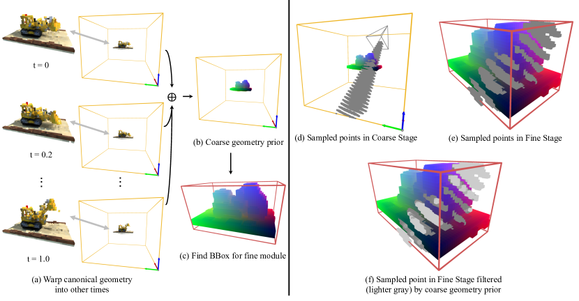
The following two strategies are used to speed up the training. First, we locate the smallest box region that fully covers the whole scene, which allows us to make full use of the grid resolution. To achieve this, we query all grid vertices of the coarse deformation feature grid in all training time steps to get the alpha values. We assume a point belongs to an object point rather than the empty space if its alpha value is larger than a predefined threshold. Using alpha values of all grid vertices at all training time steps, we could find the smallest bounding box for the dynamic scene.
Second, we filter out the sampled points in a ray if they are recognized as empty points, reducing the query numbers to the light-weight MLP. For sampled points in the deformation module, as we assume empty points to be static, we filter out sampled points whose alpha is always below a threshold during all training times. For sampled points in the canonical module, we only filter out the empty points at the canonical time.
1.2 Fine Model Design
The MLP architecture of deformation module in the fine model is the same as in the coarse model, such that the trained network weights in the coarse deformation module can be used for initializing the fine model. We initialize the deformation feature grid with the optimized feature grid in the coarse model by interpolation. This initialization can result in higher performance and shorten the training time.
We model the view-dependent effect in the fine model by using a light-weight MLP to decode the interpolated color feature. We also use a progressive scale training, which doubles the voxel resolution after some training iterations [sun2021direct].
1.3 Network Architecture
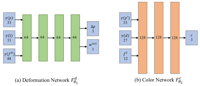
We show the architecture of our networks in Fig. 1. For deformation network , we use four layers of fully connected layer with the width set to 64. For the input layer, the dimensions of position, time and feature are 33, 11 and 44.
For the color network , we use three layers of fully connected layer with the width set to 128. For the input layer, the dimensions of position, view direction, and feature are 33, 27 and 12. Between the fully connected layer, we use ReLU as activation functions. For the occlusion output and color output , we apply sigmoid activation to transfer outputs into range of .
1.4 Hyper-parameter Settings in Experiments
As described in Eq. (16) of the paper, the overall loss function for the coarse stage and the fine stage can be written as
| (1) |
where , , , and are weights to balance each component.
In the coarse stage, we empirically set , , , and to 0.1, 0.01, 0.1, and 1, respectively. In the fine stage, these four weights were set to be smaller values as 0.01, 0.001, 0.01, and 1, respectively. As the motions of ‘Hell Warrior’, ‘Jumping Jacks’ and ‘T-Rex’ are larger, we used a smaller weight for the deformation norm regularization, with equals to and for the coarse and fine stage.
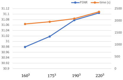
As shown in Fig. 2, the PSNR generally increase slightly after 20k iteratins, but will takes significantly more iterations to reach the max. To balance the PSNR and time consumption, we set the training iteration to 20k.

1.5 Discussion of Tips to Speed Up Training
The purpose to use coarse-to-fine training is that we could get a relative good geometry and motion model quickly and other strategy like empty-space filtering is built on this coarse model to save training time in fine stage. In Table 1, does not use any speed-up strategies and directly optimizes fine model without filtering. Under this setting, training speed, render speed and PSNR are all clearly worse than our full model . On the other hand, the train speed of is on the same level with , which means these tips are not the main factors to speed up training.
| Metrics | DNeRF | NDGV | NDGV | NDGV | NDGV |
| (half) | (half) | (full, w/o filter) | (full, w/o grid) | (full) | |
| train speed (s/scene) | 99034 | 1380 | 2487 | 1450 | 2087 |
| render speed (s/image) | 8.7 | 0.4 | 3.5 | 1.3 | 1.7 |
| model size (M) | 13.2 | 995.8 | 988.3 | 668.1 | 994.2 |
| PSNR | 30.02 | 30.32 | 27.85 | 30.62 | 31.08 |
| w/o filter: without any filter methods | w/o grid: without deformation grid | ||||
1.6 Illustration of Empty Space Filtering
As described in Section 4.2 of the paper, we speed up the training with the empty space filtering strategy. Here, we visualize our empty space filtering strategy in Fig. 3. We first locate the smallest box region that fully covers the whole scene, which is denoted as coarse geometry prior (see Fig. 3 (a)-(c)). We obtain the coarse geometry prior by warping object points in a canonical space into all other times, so that we can identify all possible positions that could be object points in the world coordinates. With this coarse geometry prior, we could reduce the volume of the grid in fine stage to avoid as many empty point as possible.
Second, we filter out the sampled points in a ray if they are recognized as empty points, reducing the query numbers to the light-weight MLP (see Fig. 3 (d)-(f)). Specifically, we filter our sampled points whose alpha values are always below a threshold during all training times. All these operations significantly reduce the time consumption of training and rendering.
2 More Analysis for the Proposed Method
2.1 Training, Rendering Speed and Model Size
We show the training and render speed of different settings in Table 1. To speed up training, we need to use a very small size MLP, which could harm the image quality. This is why we use a deformation feature grid to embed more information without adding too much complexity to the system. We can see that adding a deformation feature grid increases the PSNR at the cost of slightly more training time and bigger model size, which we believe is reasonable to balance these metrics.
We report model size in Table 1. The model size of DNeRF is the smallest thanks to the compact representation of MLP, but it doesn’t mean it is faster and cheaper to train. In fact, we could train faster on the same device compared with DNeRF and set a much bigger batch size with a resolution of around in our experiments.
In addition, We further show the training speed of each submodule in our system in Table 2. According to Table 2, we can notice a dramatic increase of time consumption of query deformation feature, deformation network forward and gradient computation process without our empty space filtering mechanism, since more empty points are involved in the optimization process without filtering.
| Methods | Deformation Module | Canonical Module | Render | Loss | Backward | Optimization | |
|---|---|---|---|---|---|---|---|
| Query Feat | Deform Net | ||||||
| NDVG (full) | 9.23e-4 | 5.06e-3 | 5.28e-3 | 1.02e-3 | 5.61e-3 | 3.50e-2 | 7.23e-3 |
| NDVG (w/o filter) | 3.28e-3 | 2.82e-2 | 4.93e-3 | 1.08e-3 | 5.36e-3 | 6.68e-2 | 7.36e-3 |
2.2 Ablation Study of Losses
| Methods | PSNR | SSIM | LPIPS |
|---|---|---|---|
| NDVG (w/o ) | 30.45 | 0.963 | 0.061 |
| NDVG (w/o ) | 31.54 | 0.971 | 0.039 |
| NDVG (full) | 31.08 | 0.970 | 0.039 |
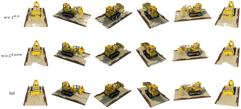
We establish the ablation study of the losses we use during training. We show the results of models trained without the total variation loss and without the deformation normalization loss in Table 3. According to Table 3, there is a significant drop without . It is worth to mention that, even it achieve slightly better results without deformation normalization loss , the geometry of canonical module degenerated due to lack of normalization of the canonical space, which is show in Fig. 4. As shown in Fig. 4, without , the canonical images are shattered without this spatial smooth term. Also, without , the canonical images are distorted. Since there are no constraints on deformation estimation, there is more freedom of the deformation between spaces at other times and the canonical space, which could cause distortions in the canonical space.
2.3 Deformation Grid Resolution
We test the different deformation grid resolution (total voxel number) and analysis the corresponding images quality and training time consumption, which is show in Fig. 5. With the total number of voxels is increasing, the overall trends of PSNR and training time consumption are also increase. We choose the final number of voxels as to balance the image quality and training time consumption.
2.4 Visualization of the Feature Grid
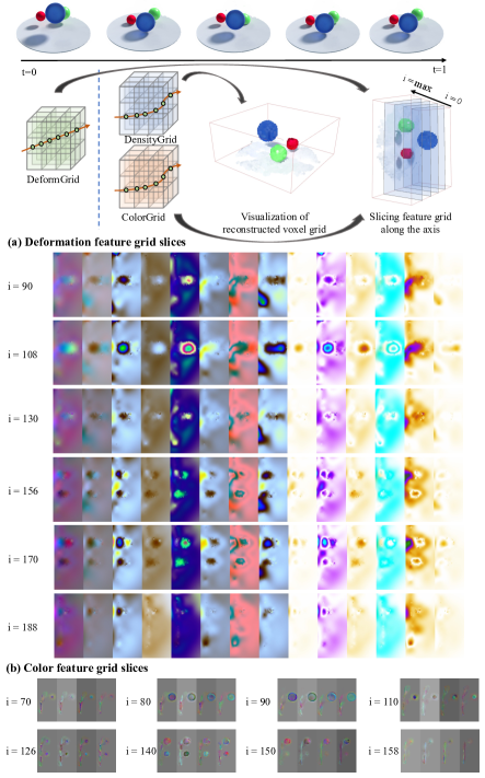
The feature grids, including deformation feature grid in Deformation Module and color feature grid in Canonical Module, play important roles in our pipeline. We show the ablation study in paper with quantitative results. Here we visualize the feature learnt from training in Fig. 6. As shown of the first row in Fig. 6, we slice the feature grid along the axis . We then treat the sliced feature slice as stacked rgb images and visualize them after normalization. In terms of deformation of feature grid slices, some of the columns (like the 4th and 5th) show clean clues of objects. Other columns (like the 6th and 7th), show clean clues of deformations of the objects (bouncing trajectory). In terms of color feature grid slices, the visualizations show clean clues of objects and no clues of movements, because it is defined in canonical space.
3 More Results
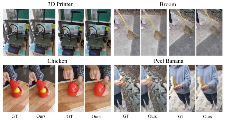
First, we show some of the test images of real scenes dataset synthesised by our method in Figure 7. The visual results demonstrate that our model could learn reasonable representation for the real dynamic scenes and enable novel view synthesis with fast optimization.
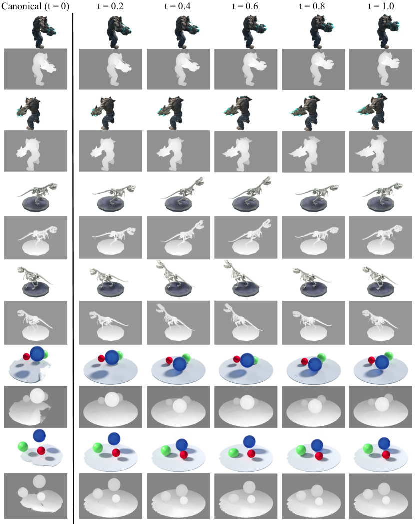
Then, we present more results for the learned geometries in Fig. 8. Our method can reconstruct accurate canonical geometry and render high-quality images for different time steps. We notice that the reconstructed canonical geometry of ‘Bouncing Balls’ has some missing parts in the white plate. One of the main reasons is that the background for this scene is white, and the plate has a color similar to the background. The image reconstruction error for this region is low even if the learned density of the plate is close to zero. Then, these low-density regions might be filtered out by our empty space filtering strategy. This problem can be easily alleviated by using a background with different color or disabling the filtering strategy.
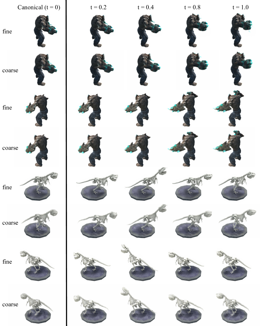
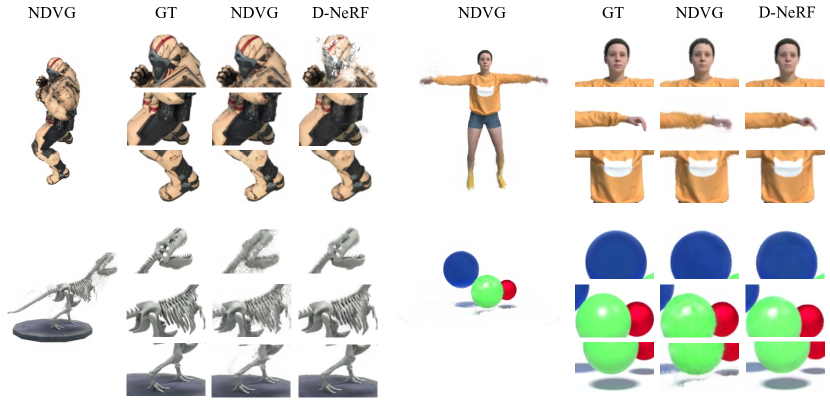
Finally, we compare the results rendered by the coarse stage and fine stage in Fig. 9, and we show more results to compare our method with D-NeRF [pumarola2021_dnerf_cvpr21] in Fig. 10.
