Deep-field Metacalibration

Abstract

We introduce deep-field metacalibration, a new technique that reduces the pixel noise in metacalibration estimators of weak lensing shear signals by using a deeper imaging survey for calibration. In standard metacalibration, a small artificial shear is applied to the observed images of galaxies in order to estimate the response the object’s shape measurement to shear, which is used to calibrate statistical shear estimates. As part of a correction for the effect of shearing correlated noise in the image, extra noise is added that increases the uncertainty on statistical shear estimates by $\sim 20$%. Our new deep-field metacalibration technique leverages a separate, deeper imaging survey to calculate calibrations with less degradation in image noise. We demonstrate that weak lensing shear measurement with deep-field metacalibration is unbiased up to second-order shear effects for isolated sources. For the Vera C. Rubin Observatory Legacy Survey of Space and Time (LSST), the improvement in weak lensing precision will depend on the somewhat unknown details of the LSST Deep Drilling Field (DDF) observations in terms of area and depth, the relative point-spread function properties of the DDF and main LSST surveys, and the relative contribution of pixel noise versus intrinsic shape noise to the total shape noise in the survey. We conservatively estimate that the degradation in precision is reduced from 20% for metacalibration to $\lesssim 5$% for deep-field metacalibration, which we attribute primarily to the increased source density and reduced pixel noise contributions to the overall shape noise. Finally, we show that the technique is robust to sample variance in the LSST DDFs due to their large area, with the equivalent calibration error being $\lesssim 0.1\%$. The deep-field metacalibration technique provides higher signal-to-noise weak lensing measurements while still meeting the stringent systematic error requirements of future surveys for isolated sources.

+

1 Introduction

Modern surveys that aim to measure weak lensing signals will constrain a wealth of fundamental physics, but in order to do so they must meet stringent requirements on the control of systematic effects (see, e.g., Mandelbaum 2018 for a review). One of the most daunting issues has been accurately measuring weak gravitational lensing shears from survey data. For the Vera C. Rubin Observatory Legacy Survey of Space and Time (LSST), these signals must be measured with systematic errors no worse than about one part per thousand to avoid degrading cosmological constraints (Huterer et al., 2006; The LSST Dark Energy Science Collaboration et al., 2018). A large number of systematic effects and measurement biases must be overcome to reach this goal, including correcting for the point-spread function (PSF), noise biases, model biases, selection effects, blending effects, and detection effects (see, e.g., Mandelbaum 2018 for a comprehensive discussion and references). So far, the community has developed three techniques that can reach the part-per-thousand accuracy required by LSST without direct calibration from image simulations. These techniques are BFD (Bernstein et al., 2016; Bernstein & Armstrong, 2014), FPFS (Li et al., 2018, 2022), and metacalibration (Sheldon & Huff, 2017; Huff & Mandelbaum, 2017), all of which meet LSST requirements for unblended, isolated sources. The newly introduced metadetection technique promises to reach part-per-thousand accuracy even in the presence of object detection and blending (Sheldon et al., 2023). The FPFS method from Li & Mandelbaum (2022) is almost as accurate in the presence of blending as well. However, much work remains to fully realize the potential of these techniques in realistic survey scenarios, including redshift-dependent shear, blending, and detection. These effects may require simulation-based calibrations (see, e.g., MacCrann et al., 2022).

Despite their success, the metacalibration and metadetection techniques as currently implemented have a nontrivial drawback. In order to reach the required accuracy in shear measurement, they effectively double the pixel noise variance in the survey images ($\sqrt{2}$ in the noise standard deviation) or equivalently reduce the signal-to-noise of every source by about 30%. As described below, this effect comes from a numerical correction needed to account for sheared pixel noise in the metacalibration pipeline. This feature results in a loss of precision in the statistical shear measurements at the $\sim 20\%$ level (Sheldon & Huff, 2017).

Interestingly, modern surveys typically have a wide-field imaging campaign, which forms the survey used for weak lensing shear measurements, and a deep-field imaging campaign, which is a much smaller region that is surveyed longer, eventually reaching exposure times of $10\times$ or more than the main wide-field survey. See for example the Dark Energy Survey deep-fields work (Hartley et al., 2022) or the planned LSST Deep Drilling Fields (DDFs) (Vera C. Rubin Observatory Website, 2022; Vera C. Rubin Observatory Community Forum, 2016; Ivezić et al., 2019). Although metacalibration currently does not take advantage of deep-field data, the BFD estimator explicitly uses it, avoiding increases in the wide-field image pixel noise in the analysis.

In this work, we propose a new technique, deep-field metacalibration, which greatly reduces noise degradation by taking advantage of a deep-field survey to derive calibrations. The standard metacalibration estimator for a mean shear has two components, the uncalibrated shape measurements $\langle\mathbf{g}\rangle$ and the mean metacalibration response matrix $\langle\mathbf{R}\rangle$, both of which are computed from the wide-field survey data. For a mean shear, these quantities are combined to form the final shear estimate as (Huff & Mandelbaum, 2017; Sheldon & Huff, 2017)

$$\hat{\gamma}\equiv\langle\mathbf{R}\rangle^{-1}\langle\mathbf{g}\rangle\ .$$

The deep-field metacalibration estimator works by computing the mean metacalibration response matrix $\langle\mathbf{R}\rangle$ from the deep-field survey data instead of the wide-field survey data. We show below that with this change, we can carefully arrange the deep-field metacalibration estimator to double the effective pixel noise variance in the deep-field survey data only. Since the deep-field survey data is lower-noise than the wide-field survey data in the first place, the final deep-field metacalibration estimator achieves higher precision than the original metacalibration technique. We find that in all cases this estimator is as accurate as the original metacalibration estimator, achieving better than part-per-thousand accuracy in the overall shear measurement for isolated sources. We demonstrate that with this new technique, we will decrease the pixel noise in metacalibration images by $\approx 30\%$, increase the signal-to-noise of metacalibration weak lensing sources and decreasing their shape noise. The exact change in the pixel noise depends in detail on the relative exposure time and PSF distributions of the wide- and deep-field surveys. We further estimate an at least $\approx 15\%$ increase in the statistical precision of weak lensing analyses with Rubin LSST due to the decreased pixel noise. We conservatively estimate that for deep-field metacalibration the uncertainty in the shear estimator is degraded by $\lesssim 5\%$ rather than the approximately 20% degradation in standard metacalibration.

The primary concern when utilizing only the deep-field data to compute the metacalibration response is sample variance. The deep-field survey typically covers a much smaller area of the sky than the wide-field survey. The metacalibration response depends on the properties of the galaxies from which it is computed (e.g., their profiles, sizes, etc.) and so will inherit sample variance in those properties due to large-scale structure. We estimate this effect with two complementary mock catalogs, finding that for the large $\approx 35$ deg² area of the LSST DDFs (Vera C. Rubin Observatory Website, 2022; Ivezić et al., 2019), the resulting sample variance scatter in the metacalibration response will be in the range of 0.05% to 0.1%. This level meets LSST requirements, and extensions of our technique that reweight the deep-field galaxy populations to match the wide-field ones may reduce this sample variance further.

Our paper is organized as follows. In Section 2, we review standard metacalibration and introduce the formalism for deep-field metacalibration. Then in Section 3, we cover the main results of our work, including tests of shear calibration (3.1) and estimates of the gains in signal-to-noise (3.2). In Section 3.3, we present a discussion of the relative importance of various corrections in the deep-field metacalibration estimator. We address the issue of sample variance in the deep-fields in Section 3.4. Finally, in Section 4, we summarize our results and suggest avenues for further research.

2 Deep-field Metacalibration Formalism

In this section, we introduce the underlying algorithms of deep-field metacalibration and describe one method to apply those algorithms to a realistic survey composed of wide- and deep-field imaging datasets. We start by examining standard metacalibration images in our formalism. We then use the intuition developed there to motivate correction terms that can be applied to the deep-field and wide-field images to enable shear measurement. Finally, we specify the details of how we combine the deep- and wide-field image sets in practice, including how to make selections on the sources and compute the deep-field metacalibration response.

For conciseness, we adopt the following notation. We denote a convolution operation of two images as $I_{1}\star I_{2}$, deconvolution as $I_{1}/I_{2}$, and pointwise addition or subtraction as $I_{1}\pm I_{2}$. We also define two special operators on images. First, we define a shearing operator $Y[I,\gamma]$ that shears the image $I$ by the shear $\gamma$. Second, we define a metacalibration operator, $M[I,N,P,P_{r}]$, defined as

$$M[I,N,P,P_{r},\gamma]=$$

$$\ \ Y[I/P,\gamma]\star P_{r}+Y[N/P,-\gamma]\star P_{r}$$

where $I$ is an image, $N$ is a second image (usually pure noise), $P$ is the image PSF, $P_{r}$ is the metacalibration reconvolution PSF, and $\gamma$ is a shear. This operator performs the standard steps of the metacalibration algorithm, including the correction for sheared noise as described in Sheldon & Huff (2017). We have not specified the exact numerical implementation of these operators for pixelated images. In practice, we rely on the galsim package which provides high-quality, performant implementations (Rowe et al., 2015). Depending on the context, these implementations rely on fast-Fourier transforms and interpolations of various kinds and orders. Our implementation is publicly available.

In what follows, we work with single images for both the wide and deep surveys. Modern surveys use a strategy of covering an area of the sky with overlapping images taken at different epochs. Multi-epoch data can be handled by forming postage stamp coadds around each object (Armstrong, R., et al., 2022) or for metadetection, by using coadds without PSF discontinuities (Becker et al., 2023; Sheldon et al., 2023). These data products have well defined PSFs, and the coadd noise properties can be determined by running pure noise images through the coaddition process. The algorithms below generalize to these multi-epoch scenarios.

2.1 Standard metacalibration

The standard metacalibration estimator is based on a linear expansion of the shape of an object, $\mathbf{e}$, in the true $\gamma$,

$$\mathbf{e} = \left.\mathbf{e}\right|_{\gamma=0}+\left.\frac{\partial\mathbf{e}}{\partial\gamma}\right|_{\gamma=0}\gamma+{\cal O}(\gamma^{2})$$

$$\equiv \left.\mathbf{e}\right|_{\gamma=0}+\mathbf{R}\gamma+{\cal O}(\gamma^{2})$$

where we have defined the response matrix $\mathbf{R}$ as

$$R_{ij}\equiv\left.\frac{\partial e_{i}}{\partial\gamma_{j}}\right|_{\gamma_{j}=0}\ .$$ (2)

Under the assumption that the intrinsic shapes of objects average to zero, $\langle\left.\mathbf{e}\right|_{\gamma=0}\rangle=0$, then we get to linear order

$$\langle\mathbf{e}\rangle\approx\langle\mathbf{R}\gamma\rangle,$$

which demonstrates that true shear is weighted by the response in the mean ellipticity. We can then calculate the response weighted mean shear

$$\hat{\gamma}\equiv\langle\mathbf{R}\rangle^{-1}\langle\mathbf{e}\rangle\approx\langle\mathbf{R}\rangle^{-1}\langle\mathbf{R\gamma}\rangle.$$ (3)

In standard metacalibration the mean response $\langle\mathbf{R}\rangle$ is computed by applying small artificial shears to the observed images of objects and using a finite difference derivative to measure how their shapes respond to the change. Including the shape measurements where no shear has been applied, this process generates five shape measurements per object. These are the one with no shear, which we denote as noshear, $\pm\epsilon_{1}$ which we denote 1p and 1m, and $\pm\epsilon_{2}$ which we denote 2p and 2m. A numerical response per object can be constructed via

$$R_{ij}\approx\frac{e_{i}^{+j}-e_{i}^{-j}}{2\epsilon}\ .$$ (4)

where we have denoted the shape measurement as $e_{i}^{\pm j}$ for the $i$th shear component with with applied shear $\pm\epsilon_{j}$ on the $j$th axis. The responses per object are typically quite noisy and so the recommended estimator for the mean shear of a region of the sky averages the response and shapes separately as above so that

$$\langle R_{ij}\rangle=\frac{\langle e_{i}^{+j}\rangle-\langle e_{i}^{-j}\rangle}{2\epsilon}\ .$$ (5)

The averages $\langle\ \rangle$ above are taken over each of the five shapes above separately after all selections have been applied in order to correct for selection effects. That is, we aggregate the shape measurements from all of the noshear images, all of the 1p images, etc. into five separate catalogs, apply the object selections to those catalogs separately, compute the average shape over those catalogs separately, and then finally compute the mean shear and response from those averaged shears. This procedure is the one described in Sheldon et al. (2020) for metadetection but applies equally well to metacalibration. However, for standard metacalibration, when using a fixed catalog, one can use separate shear and selection responses with a single set of selections as done in Sheldon & Huff (2017). When applied to isolated objects, this technique can achieve the part-per-thousand accuracy required by LSST (Huff & Mandelbaum, 2017; Sheldon & Huff, 2017).

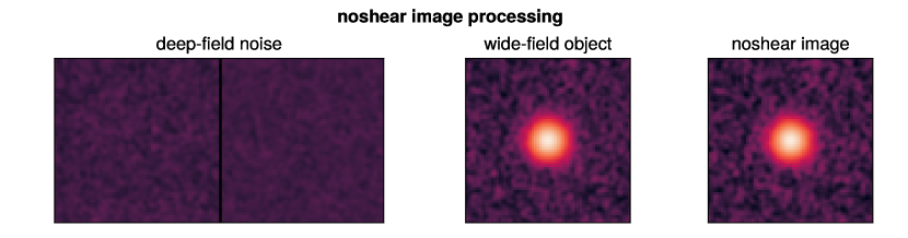
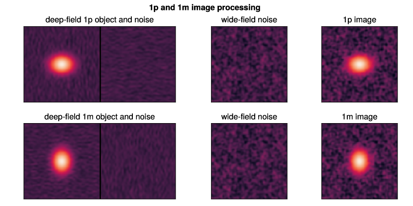
Figure 1: Deep-field Metacalibration Image Processing for the noshear, 1p, and 1m Cases. The top, middle, and bottom rows show the noshear, 1p, and 1m cases respectively. In the 1p and 1m cases, we have exaggerated the artificial shear applied to the image. The left column shows the pair of images with the deep-field noise level, either $C_{w}$ for the noshear case or $M[I_{d},N_{d}^{\prime},P_{d},P_{r},\epsilon]$ for the 1p and 1m cases. The middle and bottom pair of images in the left column clearly show the anisotropically correlated noise induced by shearing the original image and the oppositely correlated noise in the correction image. The middle column shows the image with the wide-field noise level, either $I_{w}/P_{w}\star P_{r}$ for the noshear case or $C_{d}$ for the 1p and 1m cases. The right column for each row shows the total image $\hat{I}_{w,d}$ created by summing the images in left and middle columns. These are the images used by deep-field metacalibration for computing the uncalibrated shear signal and its response.

The numerical implementation of standard metacalibration has two key features which are relevant to the discussion of deep-field metacalibration below. First, in order to artificially shear an image, one must first deconvolve the PSF. This procedure is most easily done in Fourier space where it is a simple division. However, numerical instabilities can arise since one ends up dividing by small numbers at Fourier modes where the original PSF is nearly zero. To rectify this, one typically reconvolves the image with a slightly larger PSF, called the reconvolution PSF, which controls these numerical instabilities by suppressing the affected Fourier modes.

Second, as discussed in Sheldon & Huff (2017), one must correct for the effects of sheared background noise when estimating the response to shear via finite differencing. When applying an artificial shear to a noisy image, the image is deconvolved and sheared, which produces an image with an anisotropic noise power spectrum. This effect, if left uncorrected, biases the shape measurements for the response images 1p, 1m, etc. relative to those from the noshear images, producing a biased shear estimator (see Equation 3). Sheldon & Huff (2017) tried a variety of schemes to correct for this effect, but settled on the following procedure. Before shape measurement under an artificial shear $\epsilon_{j}$, a pure noise image with the same noise spectrum as the original image is rotated by 90 degrees, put through the same deconvolution plus shearing plus reconvolution process, rotated back, and then added to the sheared original image. This procedure has the net effect of applying a shear of $-\epsilon_{j}$ to the noise image, but works even for distorted images. As detailed below, this procedure cancels the biases in the shape measurements but has the net effect of doubling the pixel noise variance in the image. It is this inefficiency we are seeking to rectify in this work.

Before describing deep-field metacalibration, it is useful to cast these two numerical operations into the notation introduced above. For this, let’s denote the galaxy as $G$, the PSF as $P$, our noise field as $N$, and the metacalibration reconvolution PSF as $P_{r}$. In this notation, the observed image of an object is $I=G\star P+N$. That is, the image of the galaxy $G$ is convolved by a PSF $P$ giving $G\star P$, and has additional noise which results in $G\star P+N$. For a shear $\epsilon$ applied the 1-axis (2-axis), we have for the noshear, 1p (2p), and 1m (2m) images

$$M[I,N^{\prime},P,P_{r},\phantom{-}0]$$

$$=Y[G,\phantom{-}0]\star P_{r}+Y[N/P,\phantom{-}0]\star P_{r}+Y[N^{\prime}/P,\phantom{-}0]\star P_{r}$$

$$M[I,N^{\prime},P,P_{r},+\epsilon]$$

$$=Y[G,+\epsilon]\star P_{r}+Y[N/P,+\epsilon]\star P_{r}+Y[N^{\prime}/P,-\epsilon]\star P_{r}$$

$$M[I,N^{\prime},P,P_{r},-\epsilon]$$

$$=Y[G,-\epsilon]\star P_{r}+Y[N/P,-\epsilon]\star P_{r}+Y[N^{\prime}/P,+\epsilon]\star P_{r}\ .$$

The first two terms of the right side of each equation arise from the deconvolution, shearing, reconvolution process applied to the original image of the object ($(G+N)\star P$). The last term on the right side is the sheared noise correction. The more formal approach of the equations above illustrates an import numerical relationship between the noise distributions in the noshear versus 1p and 1m (or 2p and 2m) images. Namely, the noshear image has noise that looks like

$$N_{\rm noshear}=Y[N/P,\phantom{-}0]\star P_{r}+Y[N^{\prime}/P,\phantom{-}0]\star P_{r}$$

whereas the 1p and 1m (or 2p and 2m) images have identical noise that looks like

$$N_{\rm 1p,2p}=Y[N/P,+\epsilon]\star P_{r}+Y[N^{\prime}/P,-\epsilon]\star P_{r}\ .$$

This set of relationships is key to canceling biases in the response do the sheared noise while also properly accounting for selection effects (Sheldon & Huff, 2017).

For deep-field metacalibration, we will need to preserve these relationships while additionally accounting for the differing PSFs and noise distributions in the wide- versus deep-field images. If we did not, then selections made on shear sources made in the deep-fields would not match the wide-fields or vice versa. Similarly, the noise biases would differ between the wide- and deep-fields, and thus ruin any response-like corrections we would attempt to make. We demonstrate how to achieve these goals next.

2.2 Deep-field Metacalibration

Before presenting the deep-field metacalibration technique in detail, it is useful to discuss general constraints on the method and to develop some intuition. First, as discussed above, we are seeking to avoid doubling the wide-field image variance. This doubling comes from corrections for numerical operations that shear pixel noise. Therefore, our final technique should avoid shearing the wide-field images. A technique which computes the shear response only from the deep-field images would satisfy this constraint. It would also allow us to easily run analyses on the wide-field shape catalog in the same way as has been done in the past (see, e.g., Gatti et al., 2021) – we’d compute our shear statistics with the wide-field shape catalog, compute the response by applying the same selections to the deep-field catalogs and applying Equation 5, and then apply the response to the data. Second, we will still need the sheared noise correction term when computing the response from the deep-fields, so we expect the final technique will double the pixel variance of the deep-field images. Third, as we just argued, we’ll need to match the PSF and noise distributions in the deep- and wide-field images in order to correctly account for common sources of bias in the shear estimates. A simple approach to match the noise distributions would be to apply a copy of the wide-field noise to the deep-field image and vice versa. Finally, we’ll need to ensure that the various manipulations of the images with the PSF are numerically stable. Given that we expect to need to match the PSFs between the deep- and wide-field images, a natural choice for a reconvolution PSF for numerical stability would be the largest of the reconvolution PSFs of either the deep- or wide-field images. deep-field metacalibration uses variants of these ideas as we show next.

The set of deep- and wide-field images, $\hat{I}_{d}$ and $\hat{I}_{w}$, that satisfies these constraints for an artificial shear $\epsilon$ is

$$\hat{I}_{w} = I_{w}/P_{w}\star P_{r}+C_{w}$$ (6)

$$\hat{I}_{d} = M[I_{d},N_{d}^{\prime},P_{d},P_{r},\epsilon]+C_{d}$$ (7)

where

$$C_{w}=M[N^{{}^{\prime\prime}}_{d},N^{{}^{\prime}}_{d},P_{d},P_{r},\epsilon=0]$$ (8)

$$C_{d}=N^{\prime}_{w}/P_{w}\star P_{r}\ .$$ (9)

Here $I_{w,d}$ are the input wide/deep-field images, $P_{w,d}$ are wide/deep-field PSFs, $N^{{}^{\prime},^{\prime\prime}}_{w,d}$ are wide/deep-field noise realizations, and $P_{r}$ is the largest reconvolution PSF between the wide- and deep-fields. Expanding these equations out we find that the noise in both images $\hat{I}_{w,d}$ can be computed as

$$\hat{N}_{\alpha}=N_{w}/P_{w}\star P_{r}+Y[N_{d}/P_{d},\alpha]\star P_{r}+Y[N^{\prime}_{d}/P_{d},-\alpha]\star P_{r}$$

with $\alpha\in\{0,+\epsilon,-\epsilon\}$. As is clear, we’ve avoided adding an extra wide-field noise image at the cost of adding two extra deep-field noise realizations, our original goal above. We’ve also matched the noise distributions in the images in the same way as standard metacalibration. Specifically, the wide-field (i.e., noshear) image has noise $\hat{N}_{\alpha=0}$, and the 1p and 1m (or 2p and 2m) images has noise $\hat{N}_{\alpha=\pm\epsilon}$. Finally, we’ve also managed to match the PSFs in the final images to $P_{r}$ and ensured numerical stability by choosing $P_{r}$ to be big enough to suppress deconvolution noise effects from either $P_{w}$ or $P_{d}$.

The deep-field metacalibration shear estimate is computed via

$$\hat{\gamma}\equiv\langle\mathbf{R}\rangle^{-1}_{\rm deep}\langle\mathbf{e}\rangle_{\rm wide}\ .$$ (10)

Specifically, one computes the deep-field metacalibration response $R$ from the deep-field image set $\hat{I}_{d}$ and the uncalibrated shear signal from the wide-field image set $\hat{I}_{w}$. In each set of images, one makes identical selection cuts and shape measurements on the objects, and then computes the average shape over the catalog of selected objects. Further details on how to generalize this procedure to a realistic survey are given in Section 2.3.

Figure 1 shows the various parts of the deep-field metacalibration images for noshear, 1p, and 1m cases. The left columm shows the pair of images with deep-field noise levels and the middle column shows parts with wide-field noise levels. The pair of images comes from the two images added together in the metacalibration process, the original image and the noise image, in order to correct for sheared background noise. The images in left and middle columns are added together to produce the final deep-field metacalibration images $\hat{I}_{w,d}$ in the right column. We have exaggerated the artificial shear $\epsilon$ so that one can see the sheared background noise and the oppositely sheared background noise correction for the deep-field metacalibration images in the last two rows of the left column.

In the top row for the noshear image, the left column shows a pair of images that, when added together, form $C_{w}$. These images add in noise levels and correlations from the deep-field image put through metacalibration. Thus effects like noise bias on the shears or selections on signal-to-noise will be the same in both the wide- and deep-field images. the middle column shows $I_{w}/P_{w}\star P_{r}$ which is the wide-field image that carries the uncalibrated shear signal but PSF-matched to the final reconvolution PSF. Remember that this reconvolution PSF $P_{r}$ is the same for both the wide- and deep-field images. Thus this term serves to bring the wide-field PSF to the final PSF of the deep-field image $\hat{I}_{d}$. The metacalibration response of a galaxy to shear depends critically on the PSF, in terms of both its value (e.g., larger galaxies relative to the PSF respond more to shear), and through more subtle effects like selection, blending, and detection. By matching the PSFs of the images, we ensure that these effects are the same in both the wide- and deep-fields.

The middle and bottom rows show the 1p and 1m cases respectively. The left column with the pair of images is the term $M[I_{d},N_{d}^{\prime},P_{d},P_{r},\epsilon]$. This term is standard metacalibration applied to the deep-field images. More explicitly, this term has the artificially sheared image and the correction for the sheared background noise. These two items are needed for proper shear response computations. The middle column shows $C_{d}$, which serves to bring the noise in deep-field metacalibration response images to the wide-field noise level so that selections and noise bias levels match between the wide- and deep-field images.

In Figure 2, we compare the correlated noise fields for the wide- and deep-field images, $\hat{I}_{w,d}$. The left and middle panels show example realizations of the noise fields. Visually, the correlation structure is similar. To test their agreement numerically, we compute the pixel-pixel correlation matrix for adjacent pixels in both images, averaging over $10^{6}$ realizations to reduce the noise. We show the difference between the wide- and deep-field pixel-pixel correlation matrices in the right panel. They agree to ${\cal O}(10^{-5})$, indicating that our numerical implementation of this technique is working well. We find similar fractional agreement in the overall pixel variance.

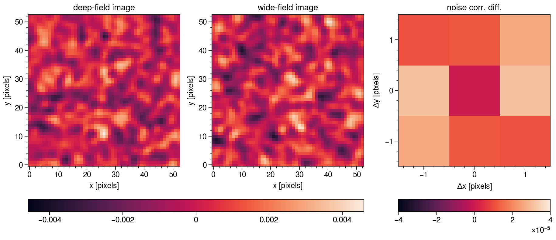
Figure 2: Left & middle panel: Example pure noise images from the deep- and wide-field image sets after deep-field metacalibration. Visually, the two noise images exhibit the same noise correlation structure. Right panel: The difference in the average pixel-pixel correlation matrix of $10^{6}$ deep- and wide-field images $\hat{I}_{w,d}$. The difference is of order $10^{-5}$, indicating good numerical performance of our codes.

2.3 Processing Realistic Sets of Wide- and Deep-field Images

In a real survey, we will have a small set of deep-field images and a larger set of wide-field images. More specifically, we won’t have a deep-field observation of every wide-field object. Thus we cannot naively apply the algorithm from the previous section to each object in the wide-field catalog in order to compute the uncalibrated shear signal and its response. Importantly, metacalibration-like estimators only require that shape measurements in the numerator for $\langle\mathbf{e}\rangle$ and the denominator for $\langle\mathbf{R}\rangle$ match statistically. This matching is in terms of not only the galaxy populations, but also the key image properties like PSF properties and noise levels. metacalibration ensures this statistical matching by using exactly the same set of objects/observations for computing $\langle{\bf R}\rangle$ and $\langle{\bf e}\rangle$. For deep-field metacalibration, we cannot rely on the wide- and deep-field image sets being statistically identical a priori. Instead, we will next devise a scheme to bring the two image sets into statistical agreement before we attempt to measure the shear signal and its response. The most obvious way in which this scheme might fail is sample variance. We estimate those effects in Section 3.4 below, demonstrating that a Rubin LSST-like survey should not be limited by sample variance.

Our scheme works as follows.

1. For every wide-field image

   1. Draw a deep-field image at random with replacement.

   2. Use Equations 6 and 8 to compute $\hat{I}_{w}$ for the noshear and use Equations 7 and 9 to compute $\hat{I}_{d}$ for the $\pm\epsilon_{1,2}$ (i.e., 1p, 1m, etc.) cases.

   3. Perform shape measurements on each of the five images (noshear, 1p, 1m, 2p, and 2m) from the last step.

   4. Accumulate a catalog of all shape measurements separately for each of the five images.

2. Apply the same set of selection cuts separately to each of the five catalogs from the last step.

3. Use the mean shapes of each of the five catalogs separately after selection in order to compute the response corrected shear via Equation 10.

This procedure is a brute-force Monte Carlo integral over the deep-field image properties for each wide-field image. More specifically, four of the five catalogs above will be of deep-field objects with properties computed from $\hat{I}_{d}$. The fifth catalog will be of wide-field objects with properties computed from $\hat{I}_{w}$. We apply the same selection cuts to all of the catalogs. The PSF and noise properties of these catalogs are statistically identical, so that these selection cuts act in the same way in both the deep- and wide-field datasets. These selection cuts can include any selection one might want to make, including tomographic binning. Thus this procedure defines how to select statistically equivalent sets of objects in the deep- and wide-fields in order to do a realistic analysis. Due to the PSF and noise matching, the overall effects of blending and source detection are the same as in standard metacalibration. Namely, there will be catastrophic shear biases for LSST-like surveys (Sheldon et al., 2020). We defer exploring these blending and detection effects to future work and focus in this work only on isolated objects, verifying that deep-field metacalibration works correctly in the same regime as metacalibration does.

In practice, there may be several avenues for improvement on the naive brute-force approach taken above. First, as we show below, deep-field metacalibration works best when the PSF of the deep-field images is the same size or smaller than the PSF of the wide-field images. Thus it may be advantageous to subselect deep-field images by their PSF size before pairing them to the wide-field images. A danger with this alternative procedure is any potential inadvertent additional selections applied to the objects that cannot be corrected by deep-field metacalibration (because they happen before deep-field metacalibration is applied). Another danger is increasing the sample variance since now effectively only a subset of the deep-field image set is used for each wide-field image. In practice, when coadded over hundreds or epochs, the wide- and deep-field images in surveys like LSST will likely have very similar, relatively narrow PSF distributions. Given that deep-field metacalibration is still effective even if the deep-field PSF is marginally bigger than the wide-field PSF, this alternative matching procedure may only supply marginal gains.

Second, the procedure defined above produces one deep-field image for every wide-field one. In practice, since the deep-field survey is smaller in area than the wide-field survey, this will mean much of the deep-field data is duplicated (but with different wide-field noise levels and reconvolution PSFs applied). It may be more efficient to separately produce much smaller deep-field image sets by using an algorithm where for each deep-field image, one selects at random a relatively small number of wide-field images to compute $C_{w}$. One must be careful to avoid extra noise from incomplete wide-field image sampling in this procedure, but this is easily tested in simulations of shear recovery. This change would produce smaller object catalogs for the deep-field measurements, making downstream manipulations of the catalogs easier.

Third and finally, we have made no attempt to reduce sample variance in the deep-field response computation by matching the properties of the wide- and deep-field objects. This matching should be possible within the deep-field metacalibration formalism. The idea is to define subsets of the wide-field objects through selection cuts on the deep-field metacalibration-computed properties. These subsets should group similar objects by size, signal-to-noise, etc. Then in the deep-field samples, one would apply the same selections to the deep-field metacalibration-computed properties. For each subset, one can compute a separate response. Then the total wide-field sample response can be computed by an appropriately weighted average of the deep-field response values. This reweighting procedure should cause no additional biases in the deep-field metacalibration shear estimator while reducing the overall sample variance in the response estimate.

One appealing aspect of deep-field metacalibration is that it naturally generalizes to metadetection. In deep-field metadetection, we process larger images through the metacalibration procedure, not just postage stamps, and perform both object detection and object shape measurement separately for all metacalibration sheared and unsheared images. For deep-field metadetection, we simply apply the same set of steps above except that we use larger images and run object detection before shape measurement. The measured object shapes are accumulated into catalogs in the same way. The response after object selections is computed in the same way as well. Further, all of the possible improvements discussed above also generalize to deep-field metadetection. This algorithm will fully handle the effects of blending and object detection. We leave explicit tests of the improvements discussed above and deep-field metadetection to future work.

Below we test a typical setup for standard metacalibration where each image is a postage stamp around a single wide- or deep-field galaxy, ignoring both detection and blending. Also, in order to separate out the effects of sample variance from our main results, we generate one deep-field image with a new galaxy chosen at random for every wide-field image, effectively working in the limit that the wide- and deep-field data cover equal but independent areas of the sky. Finally, we work in the limit of perfectly known PSF and noise properties for the deep- and wide-field images, as has been the standard in past works (see, e.g., Sheldon & Huff, 2017; Sheldon et al., 2020, 2023; Li et al., 2018; Li & Mandelbaum, 2022). Future work should carefully consider the effects of PSF and noise misestimation errors for a realsitic survey analysis pipeline.

3 Results

In this section we present our main results. These include tests of shear recovery (Section 3.1, Table 1) and estimates for how effective the technique is at reducing noise as a function of the relative exposure times and PSF sizes of the wide- and deep-field images (Section 3.2, Figure 3). We discuss the relative importance of the various correction images used by deep-field metacalibration in Section 3.3. We conclude by estimating the effects of sample variance on our estimator using two complementary simulated models of galaxy populations (Section 3.4, Figure 4).

Table 1: Shear Calibration Results for Deep-field Metacalibration

case	noisea	PSFb	galaxyc	m [$10^{-3}$, $3\sigma$ error]	c [$10^{-4}$, $3\sigma$ error]
1	fixed	fixed Gaussian	exponential	$0.37\pm 0.17$	$\phantom{-}0.09\pm 1.38$
2	variable	fixed Gaussian	exponential	$0.36\pm 0.23$	$-0.62\pm 1.77$
3	variable	variable Gaussian	exponential	$0.30\pm 0.20$	$\phantom{-}0.15\pm 0.90$
4	variable	variable Gaussian	WeakLensingDeblending	$0.53\pm 0.39$	$-0.22\pm 0.64$
5	fixed	fixed Moffat	exponential	$0.43\pm 0.20$	$\phantom{-}0.09\pm 1.28$
6	variable	fixed Moffat	exponential	$0.14\pm 0.21$	$\phantom{-}0.18\pm 1.36$
7	variable	variable Moffat	exponential	$0.38\pm 0.22$	$\phantom{-}0.68\pm 0.94$
8	variable	variable Moffat	WeakLensingDeblending	$0.53\pm 0.37$	$\phantom{-}0.00\pm 0.64$

• All simulations use a deep-field exposure time that is on average $10\times$ more than the wide-field. fixed noise uses a fixed noise level for the wide- and deep-field images, such that the deep-field noise level is a factor of $1/\sqrt{10}$ lower than the wide-field noise level. variable noise applies an additional uniform random factor between 0.9 and 1.1 to the noise levels of the both the wide- and deep-field images.

• The fixed PSF model assumes the wide- and deep-field PSFs are fixed Gaussian or Moffat profiles with FWHMs of 0.9” and 0.7” respectively. The variable PSF model assumes the wide- and deep-field PSFs are both Gaussian or Moffat profiles with FWHMs drawn from uniform distributions between 0.8” to 1.0” and 0.6” to 0.8” respectively.

• The exponential galaxy model is an object with an exponential profile with half-light radius of 0.5”. The WeakLensingDeblending model draws bulge+disk objects to match an LSST-like survey using the WeakLensingDeblending package (Sanchez et al., 2021; Kirkby, D. and Mendoza, I., and Sanchez, J., 2020).

3.1 Shear Recovery

In order to test shear recvovery, we simulate objects in postage stamps using the galsim package. The wide- and deep-field objects parameters are drawn from the same distributions and we work in the limit of an unlimited amount of deep-field data in order to reduce the noise and test the intrinsic accuracy of our methods. We further use the techniques from Pujol et al. (2019) to cancel the pixel-noise in the simulations by generating pairs of deep- and wide-field objects with the same pixel-noise but opposite true shears. See Sheldon et al. (2020) for an explicit discussion of how these techniques are applied to metacalibration and metadetection. All shape measurements are done with a post-PSF 1.2” Gaussian weighted moment. We keep only objects with signal-to-noise greater than ten and $T/T_{\rm psf}>1.2$, where $T=\sigma_{x}^{2}+\sigma_{y}^{2}$ from the moment measurement of the galaxy or PSF. We report our results in terms of the standard additive and multiplicative bias parametrization (see, e.g., Heymans et al., 2006)

$$g_{\rm meas}=(1+m)g_{\rm true}+c$$

where $m$ is the multiplicative bias and $c$ is the additive bias. All reported errors are $3\sigma$.

We present the results of our shear recovery tests in Table 1 for various cases. We have introduced additional complications into the process in a staged fashion in order to ensure we can identify the source of biases, even if they may cancel to some degree in our final results. We start with case 1, a simple setup using exponential galaxies with half light radius of 0.5”, a Gaussian PSF with FWHM 0.9” for the wide- field images, and a Gaussian PSF with FWHM 0.7” for the deep-field images. The noise level is set to generate objects with a typical signal-to-noise of $\approx 19$ for the wide-field images. The deep-field images are set to have 10$\times$ less noise variance than the wide-field images ($\sqrt{10}$ smaller standard deviation). Both the wide- and deep-field images are $53\times 53$ postage stamps with a 0.2” pixel scale. We find that our techniques can recover the true shear correctly ($m=0.37\pm 0.17$ [$10^{-3}$, $3\sigma$ error], $c=0.09\pm 1.38$ [$10^{-4}$, $3\sigma$ error]) up to second-order shear effects which are expected to be a few parts in ten thousand (Sheldon & Huff, 2017; Sheldon et al., 2020).

For case 2, we add variations in the noise levels within the wide- and deep-field samples. For this test case, we use the same setup as the previous test case, but scale the wide- and deep-field noise levels by a random uniform draw between 0.9 and 1.1. This additional test case serves to ensure that we are correctly matching the image noise properties with our technique. If we did not match the noise properties precisely, we’d expect to see biases in our results. We again find results consistent with second- order shear effects, getting $m=0.36\pm 0.23$ [$10^{-3}$, $3\sigma$ error] and $c=-0.63\pm 1.77$ [$10^{-4}$, $3\sigma$ error].

Case 3 introduces PSF size and shape variations into the previous noise variations test case. For this we draw the wide- field PSF FWHM from a uniform distribution between 0.8” and 1.0”. The deep-field PSF FWHM is drawn from a uniform distribution between 0.6” and 0.8”. We also apply a small random shear to the PSFs, drawn uniformly between -0.02 and 0.02 for each component. This test case ensures that we are appropriately PSF matching the wide- and deep-field samples. If the PSF sizes or shapes were mismatched, we’d expect to see increased multiplicative and additive biases. Again we find results consistent with second-order shear effects, getting $m=0.30\pm 0.20$ [$10^{-3}$, $3\sigma$ error] and $c=0.14\pm 0.90$ [$10^{-4}$, $3\sigma$ error].

For case 4, we introduce a population of realistic galaxies. This test case serves to ensure that the statistical matching of wide- and deep-field objects and noise properties via the procedure in Section 2.3 is working correctly. For this case we use the same setup as the last simulation but replace our exponential galaxies with randomly drawn bulge+disk objects from the WeakLensingDeblending package (Sanchez et al., 2021; Kirkby, D. and Mendoza, I., and Sanchez, J., 2020) . We match the wide-field noise level to a 10-year LSST survey, applying a uniform variation factor between 0.9 and 1.1 as before. The deep-field exposure time is set to be 10$\times$ more than the wide-field and to the image noise is scaled by a factor of $1/\sqrt{10}$. The deep-field noise level is also varied uniformly by a factor between 0.9 and 1.1. Unlike the previous cases, we simulate the deep-and wide-field images using $73\times 73$ postage stamps with the same 0.2” pixel scale. The increased image dimension allows for the larger objects in the WeakLensingDeblending catalog. We again find results consistent with second-order shear effects, with $m=0.57\pm 0.39$ [$10^{-3}$, $3\sigma$ error] and $c=-0.13\pm 0.64$ [$10^{-4}$, $3\sigma$ error]. This test neglects the effects of sample variance since we have drawn one deep-field galaxy for every wide-field galaxy. We will explore the effects of sample variance in Section 3.4 below.

Finally, we have repeated the tests above with Moffat profiles from the galsim package. We use a shape parameter $\beta=2.5$ and the same range of PSF FWHM values for each case. The Moffat profile has larger tails than a Gaussian and so serves to test the effectiveness of our reconvolution kernel algorithms. The results of these tests are listed as cases 5-8 in Table 1. We again find no biases beyond second-order shear effects.

3.2 Effectiveness as a function of Relative PSF Size and Exposure Time

Now that we have established the accuracy of our technique, we turn our attention to the expected gains in realistic survey scenarios where deep field can have larger PSFs than the wide field, and when the relative exposure times of the wide- and deep-fields vary.

We first show results for the PSF variation. For this setup, we simulate exponential galaxies with half light radii of 0.7” with the wide-field PSF size varying between 0.7” and 1.1”. We take the deep-field to have $10\times$ the exposure time of the wide-field and vary the ratio of the deep-field to wide-field PSF size from 0.5 to 1.5. The rest of the simulation parameters follow case 1 above in Section 3.1. For each configuration, we measure the ideal signal-to-noise of our galaxy, the signal-to-noise with standard metacalibration, and the signal-to-noise with deep-field metacalibration. We define the ideal signal-to-noise as that from the original wide-field image of the object with no metacalibration or deep-field metacalibration operations applied.

The results of this test are shown in the left panel of Figure 3, where we plot the signal-to-noise in units of the ideal signal-to-noise. The dashed horizontal lines at the bottom of the figure show the results of standard metacalibration. The colored shading in the lines shows results for PSF FWHMs varying between 0.7” and 1.1”. As expected for the fixed, post-PSF aperture moments employed in this work, larger PSF sizes reduce the overall signal-to-noise. The solid lines show the results of deep-field metacalibration. When the deep-field PSF is of the same size or smaller than the wide-field PSF, we see substantial gains in the signal-to-noise. This gain matches our expectations from the math above. The signal-to-noise for deep-field metacalibration is about 30% higher than for metacalibration, $0.85/0.65\approx 1.3$, when comparing the dashed and solid lines on the left side of the plot. For this ratio of signal-to-noise measures, we expect $\sqrt{2\sigma^{2}_{w}/(\sigma^{2}_{w}+2\sigma^{2}_{d})}=\sqrt{2/(1+2/10)}\approx 1.30$ since deep-field metacalibration trades one copy of the wide-field noise $\sigma^{2}_{w}$ for two copies of the deep-field noise $\sigma^{2}_{d}$. Notice however that even in the case where the deep-field PSF is moderately larger than the wide- field PSF, deep-field metacalibration is still lower noise than standard metacalibration. The average increase in signal-to-noise per object will result in weak lensing samples from deep-field metacalibration that extend to higher redshift than those from standard metacalibration. We leave estimating the amplitude and significance of this effect to future work.

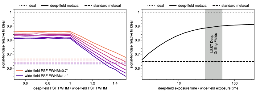
Figure 3: Left panel: Signal-to-noise relative to ideal of sources processed deep-field and standard metacalibration as a function of the ratio of deep-field PSF FWHM to the wide-field FWHM. We assume the deep-field has 10$\times$ the exposure time of the wide-field for this plot. The different colored solid lines show various wide-field PSF FWHMs ranging from 0.7” to 1.1” for deep-field metacalibration. The lower dashed lines of different colors show the result at the same wide-field PSF FWHM for standard metacalibration. The dotted line is the ideal result of one. Right panel: Signal-to-noise relative to ideal of sources processed with deep-field metacalibration and standard metacalibration as a function of the relative exposure time of the deep- versus wide-field observations. The FWHMs of the PSFs are fixed at 0.9” and 0.7” for the wide and deep images. The solid line shows deep-field metacalibration and the lower dashed line shows standard metacalibration. The dotted line is the ideal result of one. The solid gray band shows the estimated relative exposure time of the LSST Deep Drilling fields compared to the main LSST survey. Notice that in both the left and right panels, the maximum signal-to-noise for deep-field metacalibration is limited to roughly 90% of the ideal case. This effect is partly due to the increased size of the metacalibration reconvolution PSF and our use of a fixed aperture moment for flux and shape measurement.

The final salient feature of the plot is that even if deep-field metacalibration is working its best, we still find the signal-to-noise to be about $10\%$ lower than the ideal case, shown as the dotted line. This feature is partly due to the increased size of the reconvolution PSF used in the deep-field metacalibration image manipulations. We have used a relatively conservative setting of the reconvolution PSF size in this work. Better techniques to set the reconvolution PSF size, like those employed in the Dark Energy Survey metacalibration shear measurements (Gatti et al., 2021) would result in smaller losses due to this effect.

Now we turn to the effects of the relative exposure time of the wide- and deep-field images. For this test, we fix the sizes of the wide- and deep- field PSFs to 0.9” and 0.7” respectively and vary the exposure time of the deep-field image from 2$\times$ to $\sim 200\times$ more than the wide-field image. The rest of the simulation parameters follow case 1 from Section 3.1. We again measure the signal-to-noise in units of the ideal signal-to-noise for our test galaxy. The results of this computation are shown in the right panel of Figure 3. The dashed line in this panel shows the results of standard metacalibration. The solid line shows the results for deep-field metacalibration. The dotted line shows the ideal result of one. We find, as expected, that as the exposure time of the deep-field image increases, our technique becomes more effective. Again we see an overall loss of $\sim 10\%$ in signal-to-noise due to the reconvolution PSF. In the gray band, we show the estimated exposure time of the LSST Deep Drilling Fields relative to the main LSST survey (DDF, Vera C. Rubin Observatory Community Forum, 2016). While the actual achieved exposure time of these fields is not known yet, for a broad range of plausible exposure times, deep-field metacalibration will be quite effective at reducing noise.

While the results in this section demonstrate the benefits of deep-field metacalibration for specific sources, the overall increase in the precision of a weak lensing analysis with deep-field metacalibration depends on the exact decreases in source shape noise and increases in the effective number density due to the reduction in pixel noise. Further, for a survey like the Rubin LSST, the exact area and exposure time the DDFs are not yet known. Similarly, we do not yet know the relative PSF properties of the DDFs versus the main LSST survey. In order to proceed, we make the following relatively conservative approximation. We assume that the subset of the DDF images with the smallest PSF sizes are used to reach an exposure time of only $10\times$ that of the main LSST survey. We then simulate objects as in case 4 above using the WeakLensingDeblending package but forcing the DDFs and the main LSST survey to have the same PSF FWHM of 0.8”. We also fix the relative exposure time between the two and neglect the PSF shape variations from case 4 to reduce noise in our estimate. For each object, we measure its shear using standard metacalibration and deep-field metacalibration. We then compute the error on the mean shear which is dictated by the same combination shape noise and effective number density that enters the cosmic shear covariance matrix (i.e. $\sqrt{\sigma_{e}^{2}/n}$ where $\sigma_{e}^{2}$ is the shape noise and $n$ is the number density of sources). We find that deep-field metacalibration achieves an $\approx 15\%$ smaller error on the mean shear relative to standard metacalibration. Note that Sheldon & Huff (2017) found that the increased pixel noise in standard metacalibration resulted in an $\approx 20\%$ overall degradation in the precision of statistical weak lensing measurements relative to an ideal case with no increased pixel noise. Our results thus suggest that the degradation is reduced to a few percent with deep-field metacalibration. As our simulations do not contain perfect realism, we conservatively estimate the degradation for deep-field metacalibration is $\lesssim 5\%$. In more realistic scenarios, we may be able to use more of the DDF data resulting in better performance. We defer more detailed estimates to future work.

3.3 Relative Importance of Different Correction Terms

In this section, we explore the relative importance of the two correction images, Equations 8 and 9. We consider a setup like case 1 above, but we remove one or both of these terms before computing the mean shear. For this case we also match the PSFs of the wide- and deep-fields, keeping them both at 0.8”. We also use sources with signal-to-noise of $\approx 12$ to accentuate the effects of differing noise on the shear calibration. We find that without the wide-field image correction term, the shear recovery is biased with $m=37.2\pm 8.1$ [$10^{-3}$, $3\sigma$ error]. Similarly without the deep-field image correction term, we again find that the shear recovery is biased with $m=-43.5\pm 2.2$ [$10^{-3}$, $3\sigma$ error]. Finally without either term, we find $m=-6.1\pm 2.2$ [$10^{-3}$, $3\sigma$ error], indicating some degree of cancellation in the various effects at play. The differing signs in the biases reflect changes in the response to shear of the numerator of the deep-field metacalibration estimator versus the denominator. When removing the extra deep-field noise applied to the wide-field image (i.e., Equation 8), the wide-field shape measurements respond more to shear than the deep-field shape measurements, generating positive biases. Similarly, without the extra wide-field noise applied to the deep-field image (i.e., Equation 9), the deep-field shape measurements respond more to shear than the wide-field ones, generating negative biases. The two effects largely cancel, but leave biases that exceed LSST requirements by a factor of several. These results indicate that in order to make high-precision shear measurements, the noise distributions in the images must be treated carefully.

3.4 Sample Variance

We now address the issue of sample variance in the deep-field dataset. The LSST DDF will cover $\approx 35$ deg² of area (Vera C. Rubin Observatory Website, 2022; Ivezić et al., 2019). In deep-field metacalibration, we compute the survey response only from the deep-field area. Thus sample variance in the galaxy populations for this area will imprint itself in the metacalibration response, effectively increasing our final error on the multiplicative bias. This effect is most easily characterized by the fractional scatter in the deep-field response $\langle R_{d}\rangle$. This fractional scatter is directly comparable to our requirements on the knowledge of the multiplicative bias $m$. For an LSST-like survey, the requirement for the final 10-year data is $m\lesssim 0.1-0.2\%$ (Huterer et al., 2006; The LSST Dark Energy Science Collaboration et al., 2018).

In order to estimate the magnitude of this effect, we have used two different structure formation models to compute the fractional scatter in the deep-field response as a function of the deep-field area. The first is the Buzzard simulation set (DeRose et al., 2019, 2021) which uses the ADDGALS (Wechsler et al., 2022) algorithm to populate low-resolution N-body simulations with galaxies as a function of luminosity and color. This method is able to provide $\approx 5,000$ deg² of mock galaxy populations. These catalogs match a variety of structure formation statistics at low redshift, but their ability to make high-redshift predictions is not fully tested. The Buzzard catalogs do not provide object shapes or sizes that correlate with large-scale structure. To add in this effect, we use a simple matching technique, the basis of which is described in Hearin et al. (2020). We apply a linear transformation to the Buzzard catalog to match the median and standard deviation of the $r-i$ and $i-z$ colors of objects in the WeakLensingDeblending catalog. To generate a specific deep-field data realization, we first select a contiguous region of some area from the Buzzard catalog. We then find the closest 100 galaxies from the WeakLensingDeblending catalog to each galaxy in the Buzzard catalog in $r-i$, $i-z$ color-color space. We then select one of the 100 closest galaxies at random, and use it in simulating our deep-field sample for this area. This process imprints sample variance in the galaxy populations from Buzzard into the WeakLensingDeblending catalog. The second model is the public CosmoDC2 (Korytov et al., 2019) catalog. It simulates a full set of galaxy properties in a 440 deg² area, including object shapes and sizes that correlate with large-scale structure. This catalog has been used extensively by the LSST Dark Energy Science Collaboration for simulating LSST-like observations (LSST Dark Energy Science Collaboration et al.(2021)LSST Dark Energy Science Collaboration (LSST DESC), Abolfathi, Alonso, Armstrong, Aubourg, Awan, Babuji, Bauer, Bean, Beckett, Biswas, Bogart, Boutigny, Chard, Chiang, Claver, Cohen-Tanugi, Combet, Connolly, Daniel, Digel, Drlica-Wagner, Dubois, Gangler, Gawiser, Glanzman, Gris, Habib, Hearin, Heitmann, Hernandez, Hložek, Hollowed, Ishak, Ivezić, Jarvis, Jha, Kahn, Kalmbach, Kelly, Kovacs, Korytov, Krughoff, Lage, Lanusse, Larsen, Le Guillou, Li, Longley, Lupton, Mandelbaum, Mao, Marshall, Meyers, Moniez, Morrison, Nomerotski, O’Connor, Park, Park, Peloton, Perrefort, Perry, Plaszczynski, Pope, Rasmussen, Reil, Roodman, Rykoff, Sánchez, Schmidt, Scolnic, Stubbs, Tyson, Uram, Villarreal, Walter, Wiesner, Wood-Vasey, & Zuntz, LSST DESC; Abolfathi et al., 2021).

For both models, we simulate the deep-field samples assuming the deep-field data has 10$\times$ more expsoure time than the wide-field data. Due to the fact that the wide-field noise is applied to the deep-fields, we cut the input simulation catalogs keeping only objects brighter than $r$-band of $26$. For this specific test, we fix the PSF FWHM to 0.7” for both the wide- and deep-field images. All images are $73\times 73$ pixel postage stamps with a 0.2” pixel scale. With this setup, we compute the fractional scatter in the shear response for a variety of assumed deep-field areas, ranging from 1 deg² to 8 deg². The results of this computation are shown in Figure 4. We find that the fractional scatter decreases approximately as $\sim 1/\sqrt{\rm area}$ as one might expect. The simulations give somewhat different results, with CosmoDC2 consistently about 0.1% higher than the Buzzard +WeakLensingDeblending model. For areas approaching that of the LSST DDF, we estimate a residual fractional scatter in the range of 0.05% to 0.1% assuming a DDF area of 35 deg² and the $1/\sqrt{\rm area}$ scaling. This level of sample variance will meet or be less than LSST requirements.

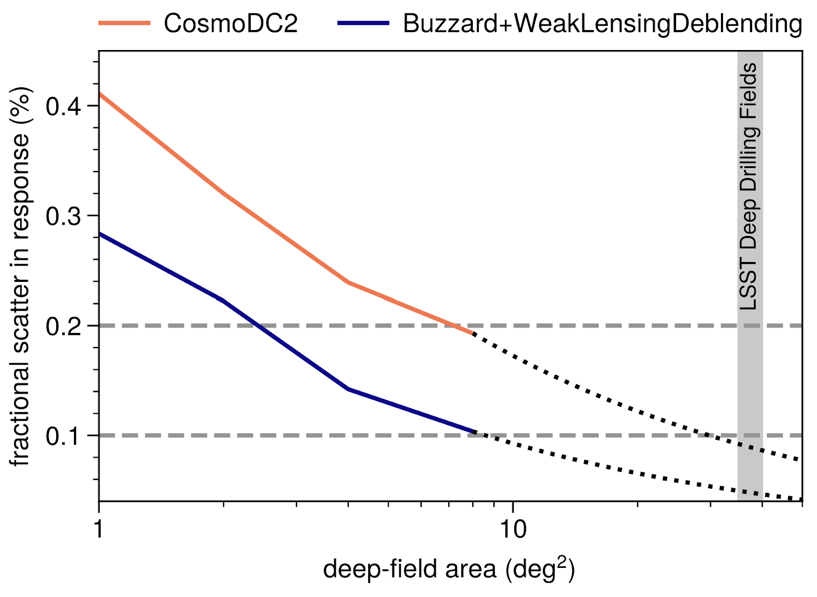
Figure 4: Sample variance scatter in the deep-field response as a function of the deep-field area. The different colored lines show the estimated sample variance from two different mock galaxy catalogs, CosmoDC2 and Buzzard +WeakLensingDeblending. The dashed lines represent the expected range of requirements on the shear calibration. The solid gray band shows the estimate area of LSST Deep Drilling Fields. The dotted lines show extrapolations to the LSST Deep Drilling Fields area assuming the sample variance scales as $1/\sqrt{\rm area}$. The LSST Deep Drilling fields will be large enough to result in sample variance scatter levels around 0.05% to 0.1%, meeting LSST requirements.

We have examined the galaxy properties of the CosmoDC2 and Buzzard +WeakLensingDeblending samples in order to understand why they give different results. We find that the CosmoDC2 model has a broader variance in the bulge-to-disk ratio while the shape noise distributions are largely similar. We also find that the CosmoDC2 catalog has a slightly higher number density of objects, with $\approx 65\ {\rm objects}/{\rm arcmin}^{2}$ as opposed to the Buzzard +WeakLensingDeblending catalogs with only $\approx 50\ {\rm objects}/{\rm arcmin}^{2}$. This difference in number density does not account for the differences in the response sample variance scatter. Whatever the exact nature of the differences between the catalogs, our current results indicate that for a broad range of assumptions about the LSST DDF samples, deep-field metacalibration will be an effective technique.

4 Summary

In this work, we have developed a new technique called deep-field metacalibration. It allows one to combine images from deep- and wide-field data sets to measure weak lensing gravitational shear using metacalibration-type methods but at higher precision. In particular our main conclusions are:

• Deep-field metacalibration allows one to combine images from wide- and deep-field surveys to measure metacalibration weak lensing shears at below part-per-thousand accuracy for isolated sources (Section 3.1, Table 1) while reducing the pixel noise in metacalibration images by $\approx 30\%$ (Section 3.2).

• The exact decrease in pixel noise depends on the details of the wide- and deep-field exposure time and PSF distributions (Section 3.2).

• When applied to the Rubin LSST, we expect an at least $\approx 15\%$ increase in the precision of weak lensing analyses due to the decreased pixel noise contributions to the shape noise and increased effective source density. We conservatively estimate that the corresponding degradation in the precision of statistical shear measurements relative to an ideal case of no extra pixel noise is reduced from 20% for standard metacalibration to $\lesssim 5\%$ for deep-field metacalibration.

• The LSST DDFs will have enough area to suppress the effects of sample variance in the deep-fields to levels that will meet LSST requirements (Section 3.4).

• Deep-field metacalibration will extend naturally to metadetection due to the fact that it explicitly matches the PSF of the deep- and wide-field images, ensuring detection and blending biases are properly calibrated (Section 2.2).

We have also discussed several avenues for improving the algorithms presented in this work. These include optimizing how one pairs the wide- and deep-field images in order to reduce signal-to-noise losses from PSF matching (Section 2.3), reducing computing costs through reducing duplication in the deep-field precessing (Section 2.3), and reducing sample variance in the deep-field response computations through reweighting the deep-field catalogs within metacalibration/metadetection to better match the wide-field object distributions (Section 2.3). Finally, it is important that this work be extended to test deep-field metadetection, in order to work out technical issues related to handling real-world effects like image coaddition, masking/artifacts, bright stars, PSF mistestimation errors, noise misestimation errors, etc. Detailed tests of deep-field metadetection will be needed to ensure our techniques can reach their full potential.

In future work, we will pursue the above improvements, perform explicit tests of deep-field metadetection for LSST-like surveys, and develop an implementation of deep-field metadetection for Rubin LSST data.

References

- Abolfathi et al. (2021) Abolfathi, B., Armstrong, R., Awan, H., et al. 2021, arXiv preprint arXiv:2101.04855
- Armstrong, R., et al. (2022) Armstrong, R., et al. 2022, in prep.
- Becker et al. (2023) Becker, M. R., Sheldon, E. S., & Jarvis, M. 2023, in prep.
- Bernstein & Armstrong (2014) Bernstein, G. M., & Armstrong, R. 2014, MNRAS, 438, 1880, doi: 10.1093/mnras/stt2326
- Bernstein et al. (2016) Bernstein, G. M., Armstrong, R., Krawiec, C., & March, M. C. 2016, MNRAS, 459, 4467, doi: 10.1093/mnras/stw879
- conda-forge community (2015) conda-forge community. 2015, The conda-forge Project: Community-based Software Distribution Built on the conda Package Format and Ecosystem, Zenodo, doi: 10.5281/zenodo.4774216
- DeRose et al. (2019) DeRose, J., Wechsler, R. H., Becker, M. R., et al. 2019, arXiv:1901.02401, arXiv:1901.02401. https://arxiv.org/abs/1901.02401
- DeRose et al. (2021) —. 2021, arXiv:2105.13547, arXiv:2105.13547. https://arxiv.org/abs/2105.13547
- Gatti et al. (2021) Gatti, M., Sheldon, E., Amon, A., et al. 2021, MNRAS, 504, 4312, doi: 10.1093/mnras/stab918
- Harris et al. (2020) Harris, C. R., Millman, K. J., van der Walt, S. J., et al. 2020, Nature, 585, 357, doi: 10.1038/s41586-020-2649-2
- Hartley et al. (2022) Hartley, W. G., Choi, A., Amon, A., et al. 2022, MNRAS, 509, 3547, doi: 10.1093/mnras/stab3055
- Hearin et al. (2020) Hearin, A., Korytov, D., Kovacs, E., et al. 2020, Monthly Notices of the Royal Astronomical Society, 495, 5040
- Heymans et al. (2006) Heymans, C., Van Waerbeke, L., Bacon, D., et al. 2006, MNRAS, 368, 1323, doi: 10.1111/j.1365-2966.2006.10198.x
- Huff & Mandelbaum (2017) Huff, E., & Mandelbaum, R. 2017, arXiv: 1702.02600. https://arxiv.org/abs/1702.02600
- Hunter (2007) Hunter, J. D. 2007, Computing in Science & Engineering, 9, 90, doi: 10.1109/MCSE.2007.55
- Huterer et al. (2006) Huterer, D., Takada, M., Bernstein, G., & Jain, B. 2006, MNRAS, 366, 101, doi: 10.1111/j.1365-2966.2005.09782.x
- Ivezić et al. (2019) Ivezić, Ž., Kahn, S. M., Tyson, J. A., et al. 2019, The Astrophysical Journal, 873, 111
- Kirkby, D. and Mendoza, I., and Sanchez, J. (2020) Kirkby, D. and Mendoza, I., and Sanchez, J. 2020, WeakLensingDeblending, 1.0.0, Zenodo, doi: 10.5281/zenodo.3975230
- Korytov et al. (2019) Korytov, D., Hearin, A., Kovacs, E., et al. 2019, The Astrophysical Journal Supplement Series, 245, 26
- Lam et al. (2015) Lam, S. K., Pitrou, A., & Seibert, S. 2015, in Proceedings of the Second Workshop on the LLVM Compiler Infrastructure in HPC, LLVM ’15 (New York, NY, USA: Association for Computing Machinery), doi: 10.1145/2833157.2833162
- Li et al. (2018) Li, X., Katayama, N., Oguri, M., & More, S. 2018, Monthly Notices of the Royal Astronomical Society, 481, 4445
- Li et al. (2022) Li, X., Li, Y., & Massey, R. 2022, Monthly Notices of the Royal Astronomical Society, 511, 4850
- Li & Mandelbaum (2022) Li, X., & Mandelbaum, R. 2022, arXiv e-prints, arXiv:2208.10522, doi: 10.48550/arXiv.2208.10522
- LSST Dark Energy Science Collaboration et al.(2021)LSST Dark Energy Science Collaboration (LSST DESC), Abolfathi, Alonso, Armstrong, Aubourg, Awan, Babuji, Bauer, Bean, Beckett, Biswas, Bogart, Boutigny, Chard, Chiang, Claver, Cohen-Tanugi, Combet, Connolly, Daniel, Digel, Drlica-Wagner, Dubois, Gangler, Gawiser, Glanzman, Gris, Habib, Hearin, Heitmann, Hernandez, Hložek, Hollowed, Ishak, Ivezić, Jarvis, Jha, Kahn, Kalmbach, Kelly, Kovacs, Korytov, Krughoff, Lage, Lanusse, Larsen, Le Guillou, Li, Longley, Lupton, Mandelbaum, Mao, Marshall, Meyers, Moniez, Morrison, Nomerotski, O’Connor, Park, Park, Peloton, Perrefort, Perry, Plaszczynski, Pope, Rasmussen, Reil, Roodman, Rykoff, Sánchez, Schmidt, Scolnic, Stubbs, Tyson, Uram, Villarreal, Walter, Wiesner, Wood-Vasey, & Zuntz (LSST DESC) LSST Dark Energy Science Collaboration (LSST DESC), Abolfathi, B., Alonso, D., et al. 2021, ApJS, 253, 31, doi: 10.3847/1538-4365/abd62c
- MacCrann et al. (2022) MacCrann, N., Becker, M. R., McCullough, J., et al. 2022, MNRAS, 509, 3371, doi: 10.1093/mnras/stab2870
- Mandelbaum (2018) Mandelbaum, R. 2018, ARA&A, 56, 393, doi: 10.1146/annurev-astro-081817-051928
- Mao et al. (2018) Mao, Y.-Y., Kovacs, E., Heitmann, K., et al. 2018, ApJS, 234, 36, doi: 10.3847/1538-4365/aaa6c3
- Pujol et al. (2019) Pujol, A., Kilbinger, M., Sureau, F., & Bobin, J. 2019, A&A, 621, A2, doi: 10.1051/0004-6361/201833740
- Rowe et al. (2015) Rowe, B. T. P., Jarvis, M., Mandelbaum, R., et al. 2015, Astronomy and Computing, 10, 121, doi: 10.1016/j.ascom.2015.02.002
- Sanchez et al. (2021) Sanchez, J., Mendoza, I., Kirkby, D. P., Burchat, P. R., & LSST Dark Energy Science Collaboration. 2021, J. Cosmology Astropart. Phys, 2021, 043, doi: 10.1088/1475-7516/2021/07/043
- Sheldon et al. (2023) Sheldon, E. S., Becker, M. R., Jarvis, M., Armstrong, R., & The LSST Dark Energy Science Collaboration. 2023, arXiv e-prints, arXiv:2303.03947, doi: 10.48550/arXiv.2303.03947
- Sheldon et al. (2020) Sheldon, E. S., Becker, M. R., MacCrann, N., & Jarvis, M. 2020, ApJ, 902, 138, doi: 10.3847/1538-4357/abb595
- Sheldon & Huff (2017) Sheldon, E. S., & Huff, E. M. 2017, ApJ, 841, 24, doi: 10.3847/1538-4357/aa704b
- The LSST Dark Energy Science Collaboration et al. (2018) The LSST Dark Energy Science Collaboration, Mandelbaum, R., Eifler, T., et al. 2018, arXiv e-prints, arXiv:1809.01669. https://arxiv.org/abs/1809.01669
- Vera C. Rubin Observatory Community Forum (2016) Vera C. Rubin Observatory Community Forum. 2016, https://community.lsst.org/t/deep-drilling-whitepapers/732
- Vera C. Rubin Observatory Website (2022) Vera C. Rubin Observatory Website. 2022, https://www.lsst.org/scientists/survey-design/ddf
- Virtanen et al. (2020) Virtanen, P., Gommers, R., Oliphant, T. E., et al. 2020, Nature Methods, 17, 261, doi: 10.1038/s41592-019-0686-2
- Wechsler et al. (2022) Wechsler, R. H., DeRose, J., Busha, M. T., et al. 2022, The Astrophysical Journal, 931, 145, doi: 10.3847/1538-4357/ac5b0a