Wide Bayesian neural networks have a simple weight posterior:
theory and accelerated sampling
Abstract
We introduce repriorisation, a data-dependent reparameterisation which transforms a Bayesian neural network (BNN) posterior to a distribution whose KL divergence to the BNN prior vanishes as layer widths grow. The repriorisation map acts directly on parameters, and its analytic simplicity complements the known neural network Gaussian process (NNGP) behaviour of wide BNNs in function space. Exploiting the repriorisation, we develop a Markov chain Monte Carlo (MCMC) posterior sampling algorithm which mixes faster the wider the BNN. This contrasts with the typically poor performance of MCMC in high dimensions. We observe up to 50x higher effective sample size relative to no reparametrisation for both fully-connected and residual networks. Improvements are achieved at all widths, with the margin between reparametrised and standard BNNs growing with layer width.
1 Introduction
Bayesian neural networks (BNNs) have achieved significantly less success than their deterministic NN counterparts. Despite recent progress (e.g., Khan et al., 2018; Maddox et al., 2019; Osawa et al., 2019; Dusenberry et al., 2020; Daxberger et al., 2021; Izmailov et al., 2021), (a) our theoretical understanding of BNNs remains limited, and (b) practical applicability is hindered by high computational demands. We make progress on both these fronts.
Our work revolves around a reparametrisation of the (flattened) NN weights . Its form comes from a theorem in which we establish that the Kullback–Leibler (KL) divergence between the standard normal distribution and the reparametrised posterior converges to zero as the BNN layers grow wide.111Case distinguishes distributions () and their densities (). Densities are used in place of distributions where convenient. This closes a gap in the theory of overparametrised NNs by providing a rigorous characterisation of the BNN parameter space behaviour (Figure 1 and Section 2), and enables faster posterior sampling (Section 3).
| parameter space | function space | |||
|---|---|---|---|---|
|
Bayesian
inference |
|
|
||
|
gradient
descent training |
|
|
In function space, wide BNN priors converge (weakly) to a so-called neural network Gaussian process (NNGP) limit (Matthews et al., 2018; Lee et al., 2018; Garriga-Alonso et al., 2019; Novak et al., 2019; Yang, 2019; Hron et al., 2020b), and the posteriors converge (weakly) to that of the corresponding NNGP (assuming the likelihood is a bounded continuous function of the NN outputs; Hron et al., 2020a). Parameter space behaviour is less understood (Hron et al., 2020a). The main exception is the work of Matthews et al. (2017) who showed that randomly initialising a NN, and then optimising only the last layer with respect to a mean squared error loss, is equivalent to drawing a sample from the conditional last layer posterior. This result holds for a Gaussian likelihood and zero observation noise. Our reparametrisation can be seen as a non-zero noise generalisation of the underlying map from the initial to the optimised weights, and provides samples from the joint posterior over all layers in the infinite width limit (Theorem 2.1).
Since sampling from the ‘KL-limit’ is trivial relative to the notoriously complex BNN posterior, our theory motivates applying Markov chain Monte Carlo (MCMC) to the reparametrised density. To apply MCMC, two concerns must be addressed: (i) understanding if the KL-closeness to actually simplifies sampling, and (ii) computational efficiency. In Section 3.1, we partially answer (i) by proving that the gradient concentrates around the log density gradient of in wide BNNs. For (ii), we propose a simple-to-implement and efficient way of computing both and the corresponding density at the same time using Cholesky decomposition (Section 3.2).
Applying Langevin Monte Carlo (LMC), we empirically demonstrate up to 50x improved mixing speed, as measured by effective sample size (ESS). The phenomenon occurs both for residual and fully-connected networks (FCNs), and for a variety of dataset sizes and hyperparameter configurations. The improvement over no reparametrisation increases with layer width, but is observed even far from the NNGP regime. For example, we find a 10x improvement on cifar-10 for a 3-hidden layer FCN with 1024 units per layer. However, for ResNet-20, a 10x improvement occurs only when the top-layer width is similar to or larger than the number of observations, illustrating that gains are possible but not guaranteed outside of the NNGP regime.
1.1 Assumptions and notation
A BNN models a mapping from inputs to outputs using a parametric function . An example is an -hidden layer fully-connected network with
| (1) |
with the nonlinearity, , and (bias terms are wrapped into by adding a constant entry dimension to ). will denote the flattened th layer parameters, and their concatenation. Later on, the vector of readout weights will be of special importance, as will the minimum hidden layer width . While we will study how the behaviour of and changes with layer width, we suppress this dependence in our notation to reduce clutter.
The factor in Equation 1 is more commonly part of the weight prior. We use this so-called ‘NTK parametrisation’ as it allows taking as the prior regardless of the network width, which simplifies our notation without changing the implied function space distribution. Our claims hold under the standard parametrisation as well, by making multiplication by a part of the reparametrisation.
We assume the final readout layer is linear, and that the likelihood is Gaussian with observation variance . In contrast, the rest of the network need not be an FCN, but can contain any layers for which NNGP behaviour is known, including convolutional and multi-head attention layers, and skip connections (see, e.g., Yang, 2020, for an overview).
2 Repriorisation: posterior prior
2.1 Repriorisation of linear models
To begin, we consider a Bayesian linear model . For a standard normal prior , the Bayesian posterior after observing points, , is a Gaussian with
| (2) |
We can thus transform a posterior into a prior sample using the data-dependent reparameterisation as illustrated in Figure 2.
| \begin{overpic}[width=57.81621pt,trim=7.02625pt 8.03pt 6.02249pt 6.02249pt]{FIGURES/lin_theta.pdf} \put(90.0,0.0){\huge$\theta$} \end{overpic} |
\begin{overpic}[width=72.26999pt,trim=3.01125pt 7.02625pt 3.01125pt 2.00749pt]{FIGURES/lin_legend.pdf}
\end{overpic}
|
\begin{overpic}[width=57.81621pt,trim=7.02625pt 8.03pt 6.02249pt 6.02249pt]{FIGURES/lin_phi.pdf} \put(90.0,0.0){\huge$\phi$} \end{overpic} |
2.2 Repriorisation of Bayesian neural networks
A similar insight applies to BNNs with the assumed Gaussian prior and likelihood. Specifically, the posterior of readout (top-layer) weights conditioned on the other parameters is with and as in Equation 2, except is replaced by the scaled top-layer embeddings . Our reparametrisation can thus be defined analogously:222 See Appendix E for discussion of alternative reparametrisations which modify parameter values in layers beyond readout.
| (3) |
This ensures for any fixed value of . We omit the dependence of , on the dataset and the pre-readout parameters to reduce clutter, but emphasise that depends on both.
Since is a differentiable bijection, the full reparametrised density is where
| (4) |
2.3 Interpreting the reparametrised distribution
To better understand the reparametrisation, note where we already know the first term is equivalent to . Since , the latter term is equal to the marginal posterior over
| (5) |
where (i) comes from completing the square (), and applying the Woodbury identity.
Using the Weinstein–Aronszajn identity
the readers familiar with the GP literature may recognise as weighted by the marginal likelihood of a centred GP with the empirical NNGP kernel (Rasmussen & Williams, 2005). The marginal likelihood is often used for optimisation of kernel hyperparameters. Here the role of the ‘hyperparameters’ is played by , i.e., all but the readout weights.
This relation to the empirical NNGP kernel is crucial in the next section where we exploit the known convergence of to a constant independent of in wide BNNs, to prove that the reparametrised posterior converges to the prior distribution at large width. Figure 4 provides an informal argument motivating that same convergence, using the language of probabilistic graphical models (PGMs).
2.4 Asymptotic normality under reparametrisation
Our reparametrisation guarantees normality of the reparametrised posterior over for any width. Section 2.3 suggests may exhibit Gaussian behaviour as well in wide BNNs, since—outside of —its posterior depends on only through the empirical NNGP kernel which is known to converge a constant as the layer width grows (see Yang, 2020, for an overview).
This is crucial in establishing our first major result: convergence of the divergence between the prior and the reparametrised posterior to zero as the number of hidden units in each layer goes to infinity.333Please refer to Appendix A for all proofs.
Theorem 2.1.
Let be the reparametrised posterior distribution defined by the density . Assume the Gaussian prior and likelihood with , and that and under the prior as .
Then as .
The assumptions (, , as ) hold for most common architectures, including FCNs, CNNs, and attention networks (Matthews et al., 2018; Garriga-Alonso et al., 2019; Hron et al., 2020b; Yang, 2020).
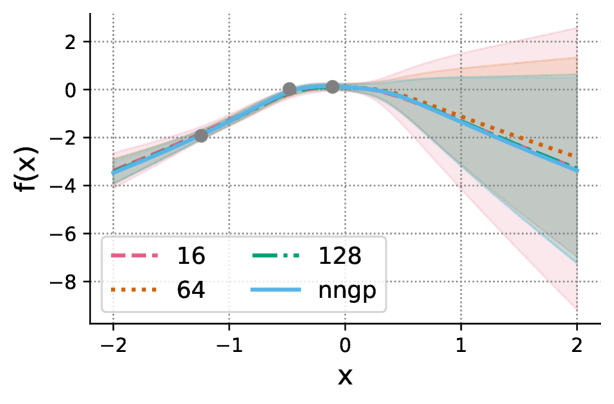
The fact that KL divergence does not increase under measurable transformations (e.g., Gray, 2011, corollary 5.2.2), combined with Theorem 2.1, implies that the KL divergence between the distribution of with and the posterior also converges to zero. This provides a simple way of approximating wide BNN posteriors as illustrated by Figure 3. We use the same argument to establish convergence in function space by showing measurability of the mapping w.r.t. a suitable -algebra.
Proposition 2.2.
Let , , and denote the functions they parametrise by and . Assume all nonlinearities are continuous, and each layer’s outputs are jointly continuous in the layer parameters and inputs.
Then as , where the is defined w.r.t. the usual product -algebra on .
Hron et al. (2020a) showed that for continuous bounded likelihoods, converges (weakly) to the NNGP posterior whenever with converges to the NNGP prior. This implies that the from Proposition 2.2 converges (weakly) to the NNGP posterior whenever does: by Pinsker’s inequality, we have convergence in total variation which implies convergence of expectations of all bounded measurable (incl. bounded continuous) functions.
Our Theorem 2.1 may moreover be seen as an appealing answer to the issue of finding a useful notion of ‘convergence’ in parameter space of an increasing dimension from (Hron et al., 2020a, section 4). As the authors themselves point out, their approach of embedding the weights in , and studying weak convergence w.r.t. its usual product -algebra, ‘tells us little about behaviour of finite BNNs’. This is most clearly visible in their proposition 2, which establishes asymptotic reversion of the parameter space posterior to the prior (without any reparametrisation), which we know does not induce the correct function space limit.
We note that our Theorem 2.1 does not contradict the Hron et al.’s result exactly because their definition of convergence essentially only captures the marginal behaviour of finite weight subsets, whereas our divergence approach characterises the joint behaviour of all the weights. Indeed, our next proposition shows that reversion to the prior does not occur under our stronger notion of convergence.
Proposition 2.3.
Under the assumptions of Theorem 2.1
as . The limit is equal to the KL divergence between the NNGP prior and posterior in function space, defined w.r.t. the usual product -algebra on .
3 Faster mixing via repriorisation
We now have a reparametrisation which provably makes the reparametrised posterior close to the standard normal prior . Since sampling from the BNN posterior is notoriously difficult, the closeness to suggests sampling from may be significantly easier.
However closeness in KL divergence does not guarantee that the gradients of are as well behaved as those of the standard normal distribution, which is crucial for gradient-guided methods like Langevin Monte Carlo (LMC). In Section 3.1, we provide partial reassurance by proving that the -norm of the differences between the two gradients vanishes in probability as the layers grow wide. Section 3.2 then provides a simple-to-implement way of computing both the reparametrised and the corresponding density at a fraction of cost of the naive implementation.
3.1 Convergence of density gradients
Our second major result proves that the posterior mass of the region where significantly differs from the gradient of the density vanishes in wide BNNs.
Proposition 3.1.
Let where is the gradient of the log density of . Assume the conditions in Theorem 2.1, and continuous nonlinearities.
Then as , .
Two more technical assumptions are in Section A.4. Albeit useful, Proposition 3.1 does not ensure gradient-guided samplers like LMC will not dawdle in regions with ill-behaved gradients. This behaviour did not occur in our experiments, but the caveat is worth remembering.
To provide a rough quantitative intuition for the scale of the speed up, we show our reparametrisation enables -times higher LMC stepsize relative to no reparametrisation in linear models, without any drop in the integrator accuracy (see Appendix D).
3.2 Practical implementation
To apply LMC, we need an efficient way of computing both and the corresponding gradient of . Since our largest experiments require millions of steps, the naive approach of computing each of , , and separately—see Equations 4 and 3— for the cost of three operations is worth improving upon. We propose a three-times more efficient alternative.
The trick is to first compute the Cholesky decomposition , and then reuse in computation of all three terms. This can be done by observing , which implies for . We can thus use the alternative reparametrisation
which uses the fact together with the above definition of . The determinant can then be computed essentially for free since
where (i) is as in Equation 4, (ii) uses standard determinant identities, and (iii) exploits that is triangular.
Because is upper-triangular, (resp. ) can be efficiently computed by back (resp. forward) substitution for any (Voevodin & Kuznetsov, 1984). The sequential application of forward and backward substitution is known as the Cholesky solver algorithm (Cholesky, 1924). Since we would need to apply the Cholesky solver to compute anyway, we obtain both the reparametrisation the density at essentially the same cost.
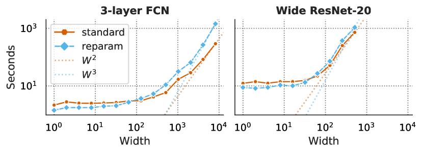
Figure 6 demonstrates our approach introduces little wall-time clock overhead on modern accelerators relative to no reparametrisation when combined with LMC. Since the per-step computational overhead is never larger than 1.5x in Figure 6 and we observe 10x faster mixing in Section 4, the cost is more than offset by the sampling speed up.
The above (‘feature-space’) reparametrisation scales as in computation and in memory. This is typically much better than exact (NN)GP inference which scales as in computation and in memory. To enable future study of very wide BNNs (), we provide an alternative ‘data-space’ formulation with computation and memory scaling in Appendix B.
Interpolating between parametrisations
We can swap the likelihood variance for a general regulariser in the definition of . Clearly, (identity mapping) as . This allows interpolation between our proposed reparametrisation at , and the standard parametrisation at , which may be useful when far from the NNGP regime. Proper tuning of the hyperparameter thus ensures the algorithm never performs worse than under the standard parametrisation.
4 Experiments
Armed with theoretical understanding and an efficient implementation, we now demonstrate that our reparametrisation can dramatically improve BNN posterior sampling, as quantified by per-step effective sample size (ESS; Ripley, 1989), and the statistics (Gelman & Rubin, 1992), over a range of architectural choices and dataset sizes.
4.1 Setup
4.1.1 diagnostic
is a standard tool for testing non-convergence of MCMC samplers. It takes collections of samples produced by independent chains, and computes
| (6) |
where and compute expectation and variance w.r.t. the empirical distribution which assigns a weight to each (conditioning on yields within-chain statistics). The numerator is just by the law of total variance, where vanishes when all chains sample from the same distribution. Values significantly larger than one thus indicate non-convergence. We follow Izmailov et al. (2021) in reporting (denoted by in their paper), instead of the square root of the above quantity. For multi-dimensional random variables, we estimate for each dimension, and report the resulting distribution over dimensions.
4.1.2 Effective sample size
ESS is a measure of sampling speed. It estimates lag autocorrelations for ( is the empirical covariance), and computes
| (7) |
The per-step ESS is then . Since estimates for high are based on only samples, we denoise by stopping the sum in Equation 7 at the first , which is the default in Tensorflow Probability’s effective_sample_size (Dillon et al., 2017).
Equation 7 is based on the identity for (population) variance of the empirical mean of i.i.d. variables Since MCMC chains produce dependent samples, estimates the number which would satisfy the above equality when substituted for under the assumption of stationarity. Because we need to estimate ESS in the very high-dimensional parameter space, we randomly choose 100 one-dimensional subspaces, project the samples, estimate ESS in each of them, and report their distribution.
4.1.3 Data and hyperparameters
The underdamped LMC sampler (Rossky et al., 1978) and cifar-10 dataset (Krizhevsky et al., 2009) are used in all experiments. We use regression on one-hot encoding of the labels shifted by so that the label mean of each example is zero, matching the BNN prior (extension to multi-dimensional outputs described in Appendix C). Gaussian likelihood with is used throughout, which we selected to ensure that (a) positive and negative labels are separated by at least , but (b) is not too small to give ourselves an unfair advantage based on the linear case intuition (Appendix D), or cause numerical issues. Sample thinning is applied in all experiments, and ESS and are always computed based on the thinned sample. However, Figures 8 and 9 visualise ESS evolution as a function of the number of LMC steps which is equal the unthinned sample size.
As common, we omit the Metropolis-Hastings correction of LMC (Neal, 1993), and instead tune hyperparameters so that average acceptance probability after burn-in stays above 98%. We observed significant impact of numerical errors on both the proposal and the calculation of the acceptance probability; we use float32 which offers significant speed advantages over float64, but can still suffer 2-5 percentage point changes in acceptance probability compared to float64 computation with the same candidate sample.
Our experiments are implemented in JAX (Bradbury et al., 2018), and rely on the Neural Tangents library (Novak et al., 2020) for both implementation of the NN model logic, and evaluation of the NNGP predictions (e.g., in Figure 3).444Code: github.com/google/wide_bnn_sampling.
4.2 Results
In Figure 5 we visualize 2D slices through the weight posterior, for the original and reparameterized network for a 1-hidden layer FCN. The log posterior is far smoother after reparametrization, and its relative smoothness improves as network width is increased relative to dataset size. As we quantify in the following sections, this enables dramatic improvements in sampling efficiency.
4.2.1 Dependence on width and dataset size
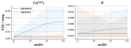
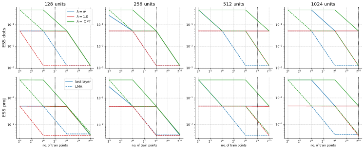
In Figure 7, we explore the dependence of mixing speed of the LMC sampler on network width and dataset size as measured by the per-step ESS. We use a single chain run of 3M steps with a 20K burn-in per each width/training set size. The results are computed on a sample thinned by a factor of 25. We use a FCN with three equal width hidden layers and GELU nonlinearities (Hendrycks & Gimpel, 2016), and the weight scaling described in Section 1.1. The weight and bias scaling factors are set to , everywhere except in the readout layer where to achieve approximately unit average variance of the network predictions under the prior (at initialisation). For the width experiments (Figure 7, left), the dataset size was fixed at , and the layer width varied over .
For each width and both parametrisations, we separately tuned the LMC stepsize and damping factor to maximise the ESS of while satisfying the mean acceptance probability criterion. For the reparametrised sampler, we also tried to tune the regularisation parameter (see Section 3.2), but found that the value dictated by our wide BNN theory () worked best even for the smallest width models. The distribution of ESS over the random projections of and on 5K test points is shown, with its mean, minimum, and maximum values.
Our reparametrisation achieves significantly faster mixing in all conditions (note the log-log scale). The improvement becomes larger as the BNN grows wider (left), achieving near-perfect values for the widest BNNs ( is maximum) where the width () is larger than the dataset (), with a 50x speed up at width 1024.
For the dataset size plots (right), the performance is again best when the ratio of width to the number of observations is the smallest (here on the left). The ESS of both and decays with dataset size as expected, since the posterior becomes more complicated, and the width to dataset size ratio dips below one, i.e., we are leaving the NNGP regime. The reparametrisation however maintains higher ESS even outside of the conditions where our theory holds.
4.2.2 Dependence on architecture
While our theory does not cover the cases where the ratio of dataset size to width is large, the consistent advantage of reparametrisation even in this regime is intriguing (Figure 7, right). In this section, we investigate the dependence of this phenomenon on the architecture and dataset size.
For the architecture, we compare the FCN from Section 4.2.1 with a normaliser-free Wide ResNet-20 with 128, 256, and 512 channels arranged from bottom to the top layer in the usual three groups of residual layer blocks (He et al., 2016; Zagoruyko & Komodakis, 2016). GELU is used for both.
As in (Izmailov et al., 2021), we remove batch normalisation since it makes predictions depend on the mini-batch, which interferes with Bayesian interpretation. We however use a different alternative in its place, namely the proposal of Shao et al. (2020), which replaces each residual sum by where is the index of the skip connection, and is a hyperparameter we set to . Since (Izmailov et al., 2021) is the closest comparison for this section, we note the authors use a categorical instead of a Gaussian likelihood555Our reparameterization also enables accelerated sampling for categorical likelihood – see Appendix F., and an i.i.d. prior for all parameters, but without scaling the weights by as we do (see Section 1.1).
For the scaling factors, FCN is as in Section 4.2.1, whereas the ResNet uses and , except in the last layer where and is again employed to ensure reasonable scale of the network predictions under the prior. As a sanity check, using this prior as initialiser, and optimising with Adam, this normaliser-free ResNet achieves a decent validation accuracy on full cifar-10. We tuned the LMC stepsize and damping factor separately for every configuration to maximise ESS of while satisfying % mean acceptance rate after burn-in. For the reparametrised chain, the regulariser was and respectively for the FCN and the ResNet, with the output variance. The sample thinning factor is 100.
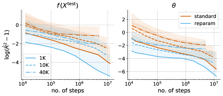
As can be seen in Figure 8, the mixing speed advantage of reparametrisation persists far from the NNGP regime in the case of the FCN (left), where even a factor of forty in dataset to width ratio did not erase the surprisingly consistent 10x higher (average) ESS. This observation is supported by Figure 9, in which is already near one (optimum) when the standard parametrisation still exhibits values.
For the Wide ResNet (right), we observed a similar 10x benefit from reparameterisation at 1K datapoints. For the 10K case, no benefit was observed. This may be because both chains are far from equilibrium even after 3M steps, and the per-step ESS measurement reflects initial transients. It may also be because the dataset size (10,240) was much larger than smallest channel count (128), exceeding by two orders of magnitude the scale where the model is expected to approximate the NNGP limit.
5 Other related work
For ensembles of infinitely-wide NNs trained with gradient descent, Shwartz-Ziv & Alemi (2020) find the KL divergence between the posterior and the prior to diverge linearly with training time, an interesting departure from the finite value we find for Bayesian inference in Proposition 2.3. The information content of infinitely-wide NNs was analysed by Bernstein & Yue (2021) using the NNGP posterior, leading to non-vacuous PAC-Bayes generalisation bounds, adding to an active line of work focusing on generalisation bounds for overparametrised models (see, e.g., Dziugaite & Roy, 2017; Valle-Perez et al., 2018; Vakili et al., 2021).
If some hidden layers are narrow and remain finite, the resulting model is a type of Deep Gaussian process (Damianou & Lawrence, 2013; Agrawal et al., 2020) or Deep kernel process (Aitchison et al., 2021). Aitchison (2020) argues that such models may exhibit improved performance relative to uniformly wide BNNs owing to a form of representation learning. While we do not investigate such questions in this work, the favourable computational properties of our LMC algorithm could facilitate such analyses in the future.
Moving away from the infinite width limit, Yaida (2020) and Roberts et al. (2021) show how to compute the Bayesian prior and posterior systematically in powers of , with the leading-order term given by the NNGP, though the subleading corrections pose computational challenges. For some architectures, a Gaussian prior in parameter space leads to closed-form expressions for the prior in function space, even at finite width (Zavatone-Veth & Pehlevan, 2021). Less is known about the posterior for finite BNNs, since computational considerations often require approximate inference, whose quality in real-world problems has recently been investigated in (Izmailov et al., 2021).
Our work is partially inspired by a thread of papers which accelerate MCMC sampling by applying an invertible transformation to a distribution’s variables, and then running sampling chains in the transformed space (e.g., El Moselhy & Marzouk, 2012; Marzouk & Parno, 2014; Parno, 2015; Marzouk et al., 2016; Titsias, 2017; Hoffman et al., 2018).
6 Conclusion
We introduced repriorisation, a reparameterisation that (1) provides a rigorous characterisation of wide BNN parameter space, and (2) enables a more efficient BNN sampling algorithm which mixes faster as the network is made wider.
Our theory shows BNN posteriors exhibit non-negligible interactions between parameters in different layers, even at large width. In contrast, many popular BNN posterior approximations (e.g., mean-field methods) assume independence between parameters in different layers. Beyond MCMC, algorithms which incorporate between-layer interactions—from Laplace (Tierney & Kadane, 1986) to more recent ones like (Ober & Aitchison, 2021)—are therefore better positioned to capture the true BNN posterior behaviour. In fairness, approximation fidelity and downstream performance are not the same thing though, as clearly demonstrated by the success of non-Bayesian approaches.
Our sampling results parallel the interplay between optimisation and model size in deterministic NNs. In particular, first-order methods used to be considered ill-suited for the non-convex loss landscapes of NNs, yet experimental and later theoretical results showed they can be highly effective, especially for large NNs (e.g., Allen-Zhu et al., 2019; Du et al., 2019). Similarly, MCMC theory tells us that sampling is often harder in high dimensions, yet our results show that a simple reparametrisation exploiting the particular structure of wide BNN posteriors makes sampling much easier.
While the gap between deterministic and Bayesian NNs remains considerable, we hope our work enables further progress for practical large-scale BNNs.
References
- Agrawal et al. (2020) Agrawal, D., Papamarkou, T., and Hinkle, J. Wide neural networks with bottlenecks are deep Gaussian processes. JMLR, 2020.
- Aitchison (2020) Aitchison, L. Why bigger is not always better: on finite and infinite neural networks. In ICML, 2020.
- Aitchison et al. (2021) Aitchison, L., Yang, A., and Ober, S. W. Deep kernel processes. In ICML, 2021.
- Allen-Zhu et al. (2019) Allen-Zhu, Z., Li, Y., and Song, Z. A convergence theory for deep learning via over-parameterization. In ICML, 2019.
- Bernstein & Yue (2021) Bernstein, J. and Yue, Y. Computing the information content of trained neural networks. arXiv, 2021.
- Billingsley (1999) Billingsley, P. Convergence of probability measures. Wiley, second edition, 1999.
- Bradbury et al. (2018) Bradbury, J., Frostig, R., Hawkins, P., Johnson, M. J., Leary, C., Maclaurin, D., Necula, G., Paszke, A., VanderPlas, J., Wanderman-Milne, S., and Zhang, Q. JAX: composable transformations of Python+NumPy programs, 2018. URL http://github.com/google/jax.
- Brooks et al. (2011) Brooks, S., Gelman, A., Jones, G., and Meng, X.-L. Handbook of Markov chain Monte Carlo. CRC press, 2011.
- Chizat et al. (2019) Chizat, L., Oyallon, E., and Bach, F. On lazy training in differentiable programming. NeurIPS, 2019.
- Cholesky (1924) Cholesky, A.-L. Note sur une méthode de résolution des équations normales provenant de l’application de la méthode des moindres carrés a un système d’équations linéaires en nombre inférieur a celui des inconnues. —application de la méthode a la résolution d’un système defini d’équations linéaires. Bulletin géodésique, 1924.
- Damianou & Lawrence (2013) Damianou, A. and Lawrence, N. D. Deep Gaussian processes. In AISTATS, 2013.
- Daxberger et al. (2021) Daxberger, E., Nalisnick, E., Allingham, J. U., Antoran, J., and Hernandez-Lobato, J. M. Bayesian deep learning via subnetwork inference. In ICML, 2021.
- Dillon et al. (2017) Dillon, J. V., Langmore, I., Tran, D., Brevdo, E., Vasudevan, S., Moore, D., Patton, B., Alemi, A., Hoffman, M., and Saurous, R. A. Tensorflow distributions. arXiv, 2017.
- Du et al. (2019) Du, S., Lee, J., Li, H., Wang, L., and Zhai, X. Gradient descent finds global minima of deep neural networks. In ICML, 2019.
- Dusenberry et al. (2020) Dusenberry, M., Jerfel, G., Wen, Y., Ma, Y., Snoek, J., Heller, K., Lakshminarayanan, B., and Tran, D. Efficient and scalable Bayesian neural nets with rank-1 factors. In ICML, 2020.
- Dziugaite & Roy (2017) Dziugaite, G. K. and Roy, D. M. Computing nonvacuous generalization bounds for deep (stochastic) neural networks with many more parameters than training data. UAI, 2017.
- El Moselhy & Marzouk (2012) El Moselhy, T. A. and Marzouk, Y. M. Bayesian inference with optimal maps. Journal of Computational Physics, 2012.
- Garriga-Alonso et al. (2019) Garriga-Alonso, A., Rasmussen, C. E., and Aitchison, L. Deep convolutional networks as shallow Gaussian processes. In ICLR, 2019.
- Gelman & Rubin (1992) Gelman, A. and Rubin, D. B. Inference from iterative simulation using multiple sequences. Statistical Science, 1992.
- Gray (2011) Gray, R. M. Entropy and Information Theory. Springer, second edition, 2011.
- He et al. (2016) He, K., Zhang, X., Ren, S., and Sun, J. Deep residual learning for image recognition. In CVPR, 2016.
- Hendrycks & Gimpel (2016) Hendrycks, D. and Gimpel, K. Gaussian error linear units (GELUs). arXiv, 2016.
- Hoffman et al. (2018) Hoffman, M., Sountsov, P., Dillon, J. V., Langmore, I., Tran, D., and Vasudevan, S. NeuTra-lizing bad geometry in Hamiltonian Monte Carlo using neural transport. AABI, 2018.
- Hron et al. (2020a) Hron, J., Bahri, Y., Novak, R., Pennington, J., and Sohl-Dickstein, J. Exact posterior distributions of wide Bayesian neural networks. UDL, 2020a.
- Hron et al. (2020b) Hron, J., Bahri, Y., Sohl-Dickstein, J., and Novak, R. Infinite attention: NNGP and NTK for deep attention networks. In ICML, 2020b.
- Izmailov et al. (2021) Izmailov, P., Vikram, S., Hoffman, M. D., and Wilson, A. G. G. What are Bayesian neural network posteriors really like? In ICML, 2021.
- Jacot et al. (2018) Jacot, A., Gabriel, F., and Hongler, C. Neural tangent kernel: Convergence and generalization in neural networks. NeurIPS, 2018.
- Khan et al. (2018) Khan, M., Nielsen, D., Tangkaratt, V., Lin, W., Gal, Y., and Srivastava, A. Fast and scalable Bayesian deep learning by weight-perturbation in Adam. In ICML, 2018.
- Krizhevsky et al. (2009) Krizhevsky, A., Hinton, G., et al. Learning multiple layers of features from tiny images, 2009.
- Lee et al. (2018) Lee, J., Sohl-dickstein, J., Pennington, J., Novak, R., Schoenholz, S., and Bahri, Y. Deep neural networks as Gaussian processes. In ICLR, 2018.
- Lee et al. (2019) Lee, J., Xiao, L., Schoenholz, S., Bahri, Y., Novak, R., Sohl-Dickstein, J., and Pennington, J. Wide neural networks of any depth evolve as linear models under gradient descent. NeurIPS, 2019.
- Levenberg (1944) Levenberg, K. A method for the solution of certain non-linear problems in least squares. Quarterly of applied mathematics, 1944.
- Maddox et al. (2019) Maddox, W. J., Izmailov, P., Garipov, T., Vetrov, D. P., and Wilson, A. G. A simple baseline for bayesian uncertainty in deep learning. In NeurIPS, 2019.
- Marquardt (1963) Marquardt, D. W. An algorithm for least-squares estimation of nonlinear parameters. Journal of the society for Industrial and Applied Mathematics, 1963.
- Marzouk & Parno (2014) Marzouk, Y. and Parno, M. Transport map-accelerated Markov chain Monte Carlo for Bayesian parameter inference. In AGU Fall Meeting Abstracts, 2014.
- Marzouk et al. (2016) Marzouk, Y., Moselhy, T., Parno, M., and Spantini, A. An introduction to sampling via measure transport. arXiv, 2016.
- Matthews et al. (2016) Matthews, A., Hensman, J., Turner, R., and Ghahramani, Z. On sparse variational methods and the Kullback-Leibler divergence between stochastic processes. In AISTATS, 2016.
- Matthews et al. (2017) Matthews, A., Hron, J., Turner, R., and Ghahramani, Z. Sample-then-optimize posterior sampling for Bayesian linear models. In AABI, 2017.
- Matthews et al. (2018) Matthews, A., Hron, J., Rowland, M., Turner, R. E., and Ghahramani, Z. Gaussian process behaviour in wide deep neural networks. In ICLR, 2018.
- Neal (1993) Neal, R. M. Probabilistic inference using Markov chain Monte Carlo methods. Technical report, University of Toronto, 1993.
- Novak et al. (2019) Novak, R., Xiao, L., Bahri, Y., Lee, J., Yang, G., Hron, J., Abolafia, D. A., Pennington, J., and Sohl-dickstein, J. Bayesian deep convolutional networks with many channels are Gaussian processes. In ICLR, 2019.
- Novak et al. (2020) Novak, R., Xiao, L., Hron, J., Lee, J., Alemi, A. A., Sohl-Dickstein, J., and Schoenholz, S. S. Neural Tangents: Fast and easy infinite neural networks in Python. In ICLR, 2020. URL https://github.com/google/neural-tangents.
- Novak et al. (2022) Novak, R., Sohl-Dickstein, J., and Schoenholz, S. S. Fast finite width neural tangent kernel. In ICML, 2022.
- Ober & Aitchison (2021) Ober, S. W. and Aitchison, L. Global inducing point variational posteriors for Bayesian neural networks and deep Gaussian processes. In ICML, 2021.
- Osawa et al. (2019) Osawa, K., Swaroop, S., Khan, M. E. E., Jain, A., Eschenhagen, R., Turner, R. E., and Yokota, R. Practical deep learning with Bayesian principles. In NeurIPS, 2019.
- Parno (2015) Parno, M. D. Transport maps for accelerated Bayesian computation. PhD thesis, MIT, 2015.
- Rasmussen & Williams (2005) Rasmussen, C. E. and Williams, C. K. I. Gaussian Processes for Machine Learning. MIT Press, 2005.
- Ripley (1989) Ripley, B. Stochastic simulation. Statistical Papers, 1989.
- Roberts et al. (2021) Roberts, D. A., Yaida, S., and Hanin, B. The principles of deep learning theory. arXiv, 2021.
- Rossky et al. (1978) Rossky, P. J., Doll, J. D., and Friedman, H. L. Brownian dynamics as smart monte carlo simulation. The Journal of Chemical Physics, 1978.
- Shao et al. (2020) Shao, J., Hu, K., Wang, C., Xue, X., and Raj, B. Is normalization indispensable for training deep neural network? In NeurIPS, 2020.
- Shwartz-Ziv & Alemi (2020) Shwartz-Ziv, R. and Alemi, A. A. Information in infinite ensembles of infinitely-wide neural networks. In AABI, 2020.
- Tierney & Kadane (1986) Tierney, L. and Kadane, J. B. Accurate approximations for posterior moments and marginal densities. Journal of the American statistical association, 1986.
- Titsias (2017) Titsias, M. K. Learning model reparametrizations: Implicit variational inference by fitting MCMC distributions. arXiv, 2017.
- Vakili et al. (2021) Vakili, S., Bromberg, M., Garcia, J., Shiu, D.-s., and Bernacchia, A. Uniform generalization bounds for overparameterized neural networks. arXiv, 2021.
- Valle-Perez et al. (2018) Valle-Perez, G., Camargo, C. Q., and Louis, A. A. Deep learning generalizes because the parameter-function map is biased towards simple functions. In ICLR, 2018.
- Voevodin & Kuznetsov (1984) Voevodin, V. and Kuznetsov, Y. Matrices and computations. Nauka, 1984.
- Wainwright (2019) Wainwright, M. J. High-dimensional statistics: A non-asymptotic viewpoint. Cambridge University Press, 2019.
- Yaida (2020) Yaida, S. Non-Gaussian processes and neural networks at finite widths. In Mathematical and Scientific Machine Learning, 2020.
- Yang (2019) Yang, G. Scaling limits of wide neural networks with weight sharing: Gaussian process behavior, gradient independence, and neural tangent kernel derivation. arXiv, 2019.
- Yang (2020) Yang, G. Tensor programs III: Neural matrix laws. arXiv, 2020.
- Zagoruyko & Komodakis (2016) Zagoruyko, S. and Komodakis, N. Wide residual networks. In BMVC, 2016.
- Zavatone-Veth & Pehlevan (2021) Zavatone-Veth, J. and Pehlevan, C. Exact marginal prior distributions of finite Bayesian neural networks. NeurIPS, 2021.
Appendix A Proofs
Here and in the main body of the paper, all statements of convergence in probability or almost sure (a.s.) convergence with necessitate construction of an underlying probability space where the random variables for network of all widths live. Since verifying that the assumptions we use are satisfied for a majority of NN architectures can be obtained by referring to the Tensor Program work of Yang, we adopt his probability space construction (e.g., Yang, 2020, appendix L).
Throughout we use the following definitions: is up to a universal positive (i.e., means s.t. ), , is the dot product, , and .
A.1 Theorem 2.1
See 2.1
Proof of Theorem 2.1.
By the conditional KL divergence identity
where the latter term is zero by the argument right after Equation 3. Recalling and
where we substituted Section 2.3 renormalised by . Note that
is a bounded function of by the positive semidefiniteness of . It is also continuous in : for the determinant use, e.g., the Leibniz formula; the matrix inverse is continuous on the space of invertible matrices by continuity of the determinant and of (sufficient here since where is positive semidefinite). Since the measure w.r.t. which we integrate is the prior , and in probability under the prior by assumption
by the definition of convergence in distribution (implied by convergence in probability), and the continuity of the .
All that remains is thus to prove
Note that the integrand is continuous in by the above argument. Using the convergence of to in probability under the prior, we thus see that the integrand converges in probability to the above constant by the continuous mapping theorem.
Convergence of the expectation can then be ensured by establishing uniform integrability (UI), and invoking the Vitali’s convergence theorem for finite measures (or theorem 3.5 in Billingsley, 1999). This is simple for the first term since
which trivially implies UI. For the log determinant, note (a.s.) by the arithmetic-geometric mean inequality. By Lemma A.1, UI integrability can thus be obtained by establishing UI of (indexed by width). Because (a.s.) and under the prior by assumption, the desired UI follows by theorem 3.6 in (Billingsley, 1999). The UI of the sum then follows by the triangle inequality. ∎
A.2 Proposition 2.2
See 2.2
Proof of Proposition 2.2.
As mentioned in the main text, KL divergence between the pushforwards of two distributions through the same measurable mapping is never larger than that between the original distributions (e.g., Gray, 2011, corollary 5.2.2). It is thus sufficient to show that for any given fixed network architecture, the mapping from the parameters into the function space is measurable with respect to the usual Borel product -algebras on and .
The product -algebra on is by definition generated by the product topology. The product topology is generated by a base composed of sets , where each is a coordinate projection associated with a point , and each is an open set in the output space . Because any finite intersection of open sets is open, it is sufficient to show that the mapping is continuous for every . Since the outputs of each layer are jointly continuous in the inputs and its own parameters by assumption, we can progress recursively from the input to the output, and conclude by observing that compositions of continuous functions are continuous. ∎
A.3 Proposition 2.3
See 2.3
Proof of Proposition 2.3.
By the conditional KL divergence identity
The first term converges to zero (see the proof of Theorem 2.1). We have also already seen (see the discussion around Equation 3). Using the formula for KL divergence between two multivariate normal distributions
where we used the Woodbury identity for the last equality. Convergence of all the above terms and their expectations has already been established in the proof of Theorem 2.1. Reintroducing the dropped constant, we therefore have
To establish equivalence to the KL between the NNGP prior and posterior, it is sufficient to employ equation (12) from (Matthews et al., 2016) with, in their notation, set to be the prior. This results in
where
by basic determinant identities. Substituting into the previous equation yields the result. ∎
A.4 Proposition 3.1
The two additional technical assumptions mentioned in the main text are:
-
1.
The set of last layer preactivations is exchangeable over the embedding (width) index, and converges in distribution to a well-defined limit (not necessarily a GP, even though that is the case in most scenarios). These facts are true for almost all architectures—(see, e.g., Matthews et al., 2018; Garriga-Alonso et al., 2019; Hron et al., 2020b; Yang, 2020).
-
2.
Defining , we assume converges as well. This will again be generally true by and theorem A.2 in (Yang, 2020).
See 3.1
Proof of Proposition 3.1.
By (see the discussion after Equation 3), the last layer gradients always exactly agree with that of the standard normal, i.e., . Hence depends only on . Substituting from Section 2.3 (after application of the Weinstein–Aronszajn identity)
We will use the shortcut to denote the derivative w.r.t. , so that . Applied to the individual summands, we have where is a vector of all ones. Similarly, . Hence the summands in both gradients have the form for some possibly random vectors whose distribution may depend on the width. Substituting the definition of
where we used the abbreviation . Therefore , so
where we have expanded the square (the last two terms are omitted as signified by the ellipsis). Defining
By Theorem 2.1, we can now integrate w.r.t. to the prior instead of the posterior , because by Pinsker’s inequality where the right-hand side goes to zero as widths go to infinity (see the proof of Theorem 2.1 for details). Using
| (8) |
by the assumed exchangeability of the readout units. By the linear readout assumption, is just a scaled version of , where is the empirical NTK, with the output layer ‘integrated out’. It thus converges in probability under the prior (and thus the posterior) by the above argument and (Yang, 2020, theorem 2.10), with going to a constant if , and to zero otherwise. Since also converges to a constant in probability (see the proof of Theorem 2.1), the vectors and do so as well. Since the vectors are just applied pointwise to the previous layer outputs, which converge to a GP by assumption, they will converge in distribution to the corresponding pushforward by the continuity of . Their limit will be denoted simply by . By the Slutsky’s lemma, the integrand thus converges in distribution to , and to zero.
Since by the outer product definition of , and the arithmetic-geometric mean inequality, it will be sufficient to establish uniform integrability (UI) of to show the expectations converge (Billingsley, 1999, theorem 3.5). This can be obtained by observing which are both non-negative random variables, which converge in probability (resp. in distribution) by continuity of the trace and the the square function. Their expectations then converge by theorem A.2 in (Yang, 2020). The collection of indexed by width is thus UI by Lemma A.1. Hence the expectations on the right hand side of Equation 8 converge, implying their sequence is bounded, and thus
Convergence in posterior probability follows by the above Pinsker’s inequality argument, and the Markov’s inequality. ∎
Auxiliary results
Lemma A.1.
If and are two collections of random variables such that for every there exists such that a.s., and is uniformly integrable (UI), then is uniformly integrable.
Proof of Lemma A.1.
Clearly by UI. Furthermore, for arbitrary , s.t.
again by the uniform integrability of . Taken together, the two facts imply is also uniformly integrable. ∎
Appendix B Feature-space vs. data-space reparametrisation
The feature-space version of our algorithm—presented in the main body and utilised in the experiments—scales cubically in the top layer width rather than the number of datapoints (cubic scaling in is the main bottleneck of exact GP inference). This is preferable in most practical circumstances since is hardly ever significantly larger than , making the additional computational overhead negligible Figure 6. Here we present a data-space version which scales cubically in as in GPs, but only quadratically in . This may be useful, e.g., when investigating properties of very wide BNNs.
The data-space version can be obtained using ideas related to the ‘kernel trick’. Starting with , we have . For the covariance
by the Woodbury identity. The reparametrisation requires the square root though, for which we can use a Woodbury-like identity for the matrix square root. To our knowledge, this identity is new and may thus be of independent interest:
| (9) |
for any and . Clearly this reduces the complexity of the square root on the l.h.s. to the complexity of the square root and matrix inverse on the r.h.s. To see the identity holds, use SVD decomposition to rewrite the l.h.s. as , and the r.h.s. as
and observe that for any . Since we need the inverse, , we can combine Equation 9 with the usual Woodbury identity for matrix inverse to obtain
We can then perform the eigendecomposition which has complexity (same as the Cholesky decomposition), and thus allows efficient computation of both , and
since is a diagonal matrix. Similar to Section 3.2, we can reuse the decomposition result to obtain the density value essentially for free using , and Equation 4 together with the Weinstein–Aronszajn identity
Appendix C Extension to multi-dimensional outputs
In the main text, we assumed the output dimension is equal to one for simplicity of exposition. The extension to is simple. In particular, we take the factorised Gaussian likelihood (see Appendix F for the categorical likelihood)
where . Each output dimension is associated with an independent readout weight s.t. . To compute , the only modification occurs in the last layer where the mean is different for each , with the th column of the targets . Importantly, is the same for all , meaning a single Cholesky decomposition is sufficient. Modern solvers allow for multi-column r.h.s. meaning that we can solve for the reparametrised value of the output weights at once, limiting the computational overhead.
The only other change is in the determinant . Because each only depends on , the determinant still has the upper-triangular structure analogous to Equation 4, implying
We can thus again re-use the result of the Cholesky decomposition to obtain the determinant value essentially for free.
Appendix D Repriorisation induced LMC speed-up in linear models
While the linear case is of course not equivalent to deep BNNs, we use it here to provide a rough intuition for the source and magnitude of the improvement that could be encountered when running LMC with instead of . To sample from a generic density , LMC (and HMC) typically uses the Leapfrog integrator to simulate the Hamiltonian dynamics of a system with potential energy and kinetic energy , where is an auxiliary momentum variable, and a positive definite mass matrix (Brooks et al., 2011).
The integrator simulates movement of a particle with initial state along a trajectory of constant energy in the ‘counter-clockwise direction’
A nice property of the linear case is that we can easily solve this matrix ODE, and thus determine the error accrued by the integrator for any given .666Whether this can be exploited to design a more efficient integrator for wide BNNs is an interesting question for future research. Without reparametrisation (), , where and . This translates into the matrix ODE
which has the usual solution
Accuracy of the integrator is thus determined by how closely it can approximate the matrix exponential . The value of this exponential is known; to simplify, we take as used in our experiments
Note that is the inverse posterior covariance, and the above equations describe a ‘rotation’ along an ellipsoid defined by the eigendecomposition of , as expected. Most importantly, the integrator error will be driven by , where in particular the LMC stepsize has to be inversely proportional to if a local approximation of and is to be accurate.
An analogous argument holds for the reparametrised version (), where by and . The stepsize can therefore be (inversely) proportional to , disregards of both and . In contrast, without the reparametrisation, the stepsize must be inversely proportional to (see above)
where we used and assumed . This assumption will be true for most sufficiently well-behaved distributions over by the law of large numbers (if exists), and the continuity of the operator norm (see chapter 6 in Wainwright, 2019, for a more detailed discussion).
In summary: without the reparametrisation, the maximum stepsize scales as , whereas it is independent of and in the reparametrised case. The higher the and/or lower the , the bigger the advantage of our reparametrisation. In the deep BNN case, we replace with , and look at the eigenspectrum of the NNGP kernel divided by (which is related to its kernel integral operator in wide enough BNNs). While only an approximation in deep BNNs, we note that a constraint of the above form must be satisfied by the sampler in order to successfully sample the readout layer (with the asymptotic NNGP replaced by the empirical one), which is why we intuitively expect the stepsize to scale at least as . This was observed in our experiments, where we indeed applied this stepsize scaling for the final hyperparameter sweep used in Figures 7 and 8.
Appendix E Alternative reparametrisations
E.1 Reparametrising other layers than readout
The reparametrisation we define in Equation 3 ensures that follows its true conditional posterior when , which we have seen is the case under . One may wonder whether there exists an alternative reparametrisation(s) which still ensures the KL divergence between and goes to zero as , but maps some other layer than the readout to its conditional posterior. In other words, is the readout ‘special’, or is mapping of any one layer to its conditional sufficient to ensure reversion to the prior in the wide limit?
For an example of a case where reparametrisation of a layer other than the readout is sufficient, consider the linear 1-hidden layer FCN with a single input and output dimension, , with respectively the input and readout weights (w.l.o.g. ). By symmetry, , implying we can apply the from Equation 3 to the input weights , and use Theorem 2.1 (mutatis mutandis) to obtain the desired KL-convergence.
However, this argument no longer holds when we introduce a nonlinearity, as the symmetry between and is broken. Moreover, we now show that the KL-convergence to the prior does not happen if we consider the only available alternative , i.e., mapping to its conditional posterior given the readout and ,777A deterministic map from prior to posterior will exist because we are in , and both prior and posterior are continuous. and leaving the readout without reparametrisation.
To start, observe that the conditional distribution of given and remains with (kernel trick), and (Woodbury identity). For simplicity, we prove that KL-convergence to prior cannot happen when the nonlinearity is bounded. Using a proof-by-contradiction, assume the KL does converge to zero. By the chain rule for KL divergence, this implies the KL between the reparametrised marginal posterior of the readout given converges in KL to the prior over , i.e., . By the assumed boundedness of and the Pinsker’s inequality, this in turn implies
However, the Pinsker’s inequality and boundedness of also imply that (prior mean), which is a contradiction unless (or ). This is not true, e.g., for the popular sigmoid non-linearity.
In summary, the answer to our question from the first paragraph is ‘it depends’. There are some linear networks in which symmetry enables reparametrising layers other than the readout and still obtaining the KL-convergence. However, introduction of non-linearities breaks this symmetry, which in turn prevents reversion to the prior. Reparametrisation of the readout is thus indeed ‘special’, as it is the only layer which ensures convergence in all cases (modulo the assumptions of Theorem 2.1).
E.2 NTK reparametrisation
Another alternative is to linearise , i.e., to use the network Jacobian to define the reparametrisation
| (10) |
This reparametrisation is inspired by the NTK theory where optimising the NN linearised around its (random) initial point by gradient descent yields the same large width behaviour as optimising the original NN (Lee et al., 2019). Informally, if (the initialisation distribution in the NTK world), and the NN is wide enough
where . By the NNGP theory, is the NNGP limit; by the NTK theory, and in probability as , where is the NTK (see, e.g., Yang, 2020, for an overview). If we approximate by substituting the limits, , we notice this is a fixed linear transformation of the NNGP, and thus also a GP. In fact, it is the NTK-GP when (Lee et al., 2019, corollary 1), i.e., the distributional limit of NNs optimised by gradient descent, where the randomness comes from the initialisation .
The above sketch shows that provides parameter-space samples which converge to the NTK-GP limit when , forming an informal NTK counterpart to Proposition 2.2. An alternative is to interpret Equation 10 as a single step of the Levenberg–Marquardt algorithm (LMA; Levenberg, 1944; Marquardt, 1963). This perspective inspired us to also experiment with multi-step LMA update (i.e., iterative application of from Equation 10) so as to adjust for potential inaccuracy of the linearisation; we also experimented with just using multiple steps of gradient descent (GD), i.e., iterative application of with a fixed . Neither the GD update nor the iterative application worked significantly better than Equation 10 in our experiments, which is why we abandon their further discussion here.
In the remainder of this section, we discuss the technical details of the NTK reparametrisation (Equation 10) implementation. Figure 10 shows a comparison of this with the ‘NNGP reparametrisation’ we presented in the main paper (Equation 3). While is sometimes competitive with , is clearly better overall. This is likely because yields samples from the NTK-GP, which may induce a complicated when the NTK-GP significantly differs from the NNGP (i.e., the correct posterior, Hron et al., 2020a). Since is also orders of magnitude more computationally efficient (scales with the top layer embedding size instead of the full parameter space dimension ), and we have rigorous understanding of its behaviour (Section 2), we do not recommend using the NTK reparametrisation. The motivation for describing it here is to inform any potential future research, documenting what we tried, and contrasting it with the NNGP reparametrisation.
E.2.1 Computing
Denoting the residuals by , becomes . Because computing costs about the same as the forward pass, and multiplication by the same as the backward pass (vector-Jacobian product), the only operations not common in standard NN training are the computation of , and the subsequent application of the linear solver .
Fortunately, the matrix , known as the empirical NTK, has recently become a subject of significant interest. We can thus use the Neural Tangents library (Novak et al., 2020) which provides a very efficient way of computing , and related matrix-vector products (Novak et al., 2022). As for the , we tried several implicit and explicit solvers, approximate and exact, but the fastest and most numerically stable was the explicit Cholesky solver. We recommend using at least float32 precision (or its emulation if on TPU) to prevent significant deterioration of the acceptance probability.
Another possible approximation is subsetting the data. Specifically, we can replace the , , and terms in by their equivalent evaluated on a fixed data subset. This may be especially tempting when computational and memory bottlenecks are an issue. One nevertheless has to be careful about designing any approximations to as—especially in the data subsetting case—these may inadvertently cause the resulting to be as constrained as , and thus erase any possible LMC speed up. For example, in the linear case, if we subset the data and some of the omitted inputs is not close to the linear span of the included ones, there will be a posterior covariance eigenvalue as low as (instead of ), which would necessitate scaling the LMC stepsize by (cf. Appendix D).
While we aim to approximate the (Equation 10), any approximation of itself is a valid reparametrisation (if bijective and differentiable), as long as the gradients and are both computed for the approximated instead of the true .
E.2.2 Approximating
Unlike above, the approximations her can affect the stationary distribution of the Markov chain or even prevent its existence. Hence the obtained samples may not be drawn from the true posterior even in the infinite time limit.
Our log determinant approximation combines the Taylor expansion of around , and the Hutchinson trick for trace estimation. In particular, for a real symmetric matrix with
| (11) |
where are i.i.d. zero mean vectors with . We use vectors with i.i.d. Rademacher entries throughout.888We tried several alternatives to including Chebyshev and learned polynomials, but did not observe a significant difference.
Unfortunately, substituting into Equation 11 would violate the symmetry requirement since
| (12) |
where is the ‘preconditioned residual’, and the Hessian at . A straightforward solution would be to use the identity . The downside is doubling of the computational time. We thus instead approximate by
| (13) |
Roughly speaking, this approximation exploits the fact that the column spaces of and in Equation 12 are close to orthogonal for small relative to . (Careful when tuning !) Rotating the space and using the block-matrix determinant formula allows us to decompose the log determinant into an asymptotically constant component aligned with the column space of , and the stochastic component .
Combining Equations 11 and 13, we have which is a symmetric matrix as desired. Furthermore, the Hutchinson estimator only requires evaluation of the vector products which can be implemented efficiently by applying the JAX vector-Jacobian function to the map where is the stop-gradient function. Finally, LMC requires estimation of the gradient but naive application of reverse-mode automatic differentiation may result in an out-of-memory (OOM) error, especially for larger architectures (the Rademacher vectors have dimension ). A more memory-efficient method is to compute both the value and gradient of the log determinant approximation in the forward pass.999Caveat: JAX allows only defining a custom , and can infer the rule automatically. However, we found it more memory efficient to explicitly define the forward pass operation, cache the computed gradient, and use the cached value to evaluate the gradient.
To illustrate, consider the second-order Taylor expansion ( in Equation 11) which we used in preliminary experiments. Exploiting the symmetry of , we define , and compute both the log determinant and its gradient as
| (16) |
where can be obtained via JAX . Since evaluating all the summands at the same time leads to OOM issues, we compute the result sequentially in a loop over mini-batches of a size smaller than .101010The first-order terms can be ignored for nonlinearities with zero second-derivative like ReLU as here.
Appendix F Non-Gaussian likelihoods