A fitted second–order difference scheme on a modified Shishkin mesh for a semilinear singularly-perturbed boundary-value problem

Abstract

In the present paper we consider the numerical solving of a semilinear singular–perturbation reaction–diffusion boundary–value problem having boundary layers. A new difference scheme is constructed, the second order of convergence on a modified Shishkin mesh is shown. The numerical experiments are included in the paper, which confirm the theoretical results.

1 Introduction

Let us consider the following boundary value problem

$$\varepsilon^{2}y^{\prime\prime}=f(x,y),\quad x\in(0,1),$$ (1)

$$y(0)=y(1)=0,$$ (2)

where $0<\varepsilon<1,$ and we assume that the nonlinear function $f$ is continuously differentiable, i.e. for $k\geqslant 2,$ $f\in C^{k}([0,1]\times\mathbb{R}),$ and that it has a strictly positive derivative with respect to $y$

$$\frac{\partial f}{\partial y}:=f_{y}\geqslant m>0,\quad(x,y)\in[0,1]\times\mathbb{R},$$ (3)

where $m$ is a constant. The problem (1)–(2) under the condition (3) has the unique solution, see Lorentz [38]. It’s a well known fact that the exact solution to the problem (1)–(3) rapidly changes near the ends points $x=0$ and $x=1.$ Also, when any classical numerical method is applied to the problem (1)–(3), then a large number of mesh points must be used to obtain a satisfactory numerical solution. It is very expensive from the computing side, and that is one of reasons for developing numerical methods which taking into account the properties of singular–perturbation boundary–value problems.

Many authors have worked on the numerical treatment of the problem (1)–(3) with different assumptions about the function $f,$ and as well as more general nonlinear problems. There were many constructed $\varepsilon$–uniformly convergent difference schemes of order 2 and higher (Herceg [10], Herceg, Surla and Rapajić [13], Herceg and Miloradović [12], Herceg and Herceg [11], Kopteva and Linß  [25], Kopteva and Stynes [27, 28], Kopteva, Pickett and Purtill [26], Linß, Roos and Vulanović [30], Sun and Stynes [42], Stynes and Kopteva [41], Surla and Uzelac [43], Vulanović [45, 46, 47, 48, 50], Kopteva [24] etc.).

In this paper we use a method introduced by Boglaev [1] to construct a different scheme, and a layer–adapted mesh introduced by Vulanović [49]. In the paper [19] the difference scheme was constructed for the same problem and the authors used the same layer–adapted mesh. It is well known fact that Shishkin mesh is the simplest layer–adapted mesh. It looks like as two uniform meshes glued, the one finer the other coarser. The simplicity of this mesh implies some simpler analysis than using other layer–adapted meshes, and that is the main benefit of using Shishkin mesh. Unfortunately, the cost of simplicity is a greater value of error.

The paper is organized as follows. The first section is Introduction, where the problem is listed and the main results. Layer–adapted mesh is 2nd section, here are given generating functions of meshes we use in this paper. A new difference scheme is constructed in section The difference scheme. Their stability is shown in the section Stability. The uniform convergence is proven in 6th section, 7th section is Numerical experiments and the last section is Conclusion.

The author’s results in numerical solving the problem (1)–(3) and others results can be seen in [7], [2], [9], [18], [19], [20], [17], [16], [23], [33], [22], [32], [8], [3], [4], [15], [5], [6], [14], [36], [37], [21], [34].

2 Layer–adapted meshes

We mentioned that classical methods are not suitable for problems like (1)–(2), before. There are several issues, with the stability, the cost of calculations and so on. These issues have been overcome by constructing special methods which take into account the presence of a layer or layers. One such a method is the fitted mesh method. Meshes that were constructed by this method have the nonuniform distribution of mesh points. The distribution of points is dictated by the behavior of the exact solution and their derivatives in a layer or layers. Estimates given in the following theorem are key to understanding of this behavior. In the following analysis we need the decomposition of the solution $y$ of the problem $(\ref{uvod1})-(\ref{uvod2})$ to a layer component $s$ and a regular component $r$, which is given in the following theorem.

Theorem 2.1.

[45] The solution $y$ to the problem $(\ref{uvod1})-(\ref{uvod2})$ can be represented in the following way:

$$y=r+s,$$

where for $j=0,1,...,k+2$ and $x\in[0,1]$ we have that

$$\left|r^{(j)}(x)\right|\leq C,$$ (4)

and

$$\left|s^{(j)}(x)\right|\leq C\varepsilon^{-j}\left(e^{-\frac{x}{\varepsilon}\sqrt{m}}+e^{-\frac{1-x}{\varepsilon}\sqrt{m}}\right).$$ (5)

Based on the previous theorem, it’s a well–known fact that the exact solution to problem (1)–(3) changes rapidly near the end points $x=0$ and $x=1.$

Many meshes have been constructed for the numerical solving problems having a layer or layers of an exponential type. In the present paper we shall use four different meshes. Let $N+1$ be the number of mesh points. These meshes $0=x_{0}<x_{1}<\ldots<x_{N}=1,$ we will get by using appropriate generating functions, i.e. $x_{i}=\psi(i/N).$ The generating functions are constructed as follows.

The first mesh is Shishkin mesh [40], the generating function for this mesh is

$$\psi(t)=\begin{cases}4\lambda t,\quad t\in[0,1/4]\\ \lambda+2(1-2\lambda)(t-1/4),\quad t\in[1/2,1/4],\\ 1-\psi(1-t),\quad t\in[1/2,1],\end{cases}$$ (6)

where $\lambda$ Shishkin mesh transition point by

$$\lambda:=\min\left\{\frac{2\varepsilon\ln N}{\sqrt{m}},\frac{1}{4}\right\}.$$ (7)

The second mesh is modified Shishkin mesh proposed by Vulanović [49], the generating function for this mesh is

$$\psi(t)=\begin{cases}4\lambda t,\quad t\in[0,1/4],\\ p(t-1/4)^{3}+4\lambda t,\quad t\in[1/4,1/2],\\ 1-\psi(1-t),\quad t\in[1/2,1],\end{cases}$$ (8)

where $p$ is chosen so that $\psi(1/2)=1/2,$ i.e. $p=32(1-4\lambda).$ Note that $\psi\in C^{1}[0,1]$ with $\|\psi^{\prime}\|_{\infty}\leqslant C,$ $\|\psi^{\prime\prime}\|_{\infty}\leqslant C.$ Therefore the mesh size $h_{i}=x_{i+1}-x_{i},\,i=0,\ldots N-1$ satisfy (see [29])

$$h_{i}=\int_{i/N}^{(i+1)N}{\psi^{\prime}(t)\operatorname{d}t}\leqslant CN^{-1},\quad|h_{i+1}-h_{i}|=\left|\int_{i/N}^{(i+1)/N}{\int^{t+1/N}_{t}{\psi^{\prime\prime}(s)\operatorname{d}s}}\right|\leqslant CN^{-2}.$$ (9)

The Shishkin mesh transition point $\lambda$ is the same as in the first Shishkin mesh, i.e. (7).

The third mesh is modified Bakhvalov mesh also proposed by Vulanović [44], the generating function for this mesh is

$$\psi(t)=\begin{cases}\mu(t):=\frac{a\varepsilon t}{q-t},\quad t\in[0,\alpha],\\ \mu(\alpha)+\mu^{\prime}(\alpha)(t-\alpha),\quad t\in[\alpha,1/2],\\ 1-\psi(1-t),\quad t\in[1/2,1],\end{cases}$$ (10)

where $a$ and $q$ are constants, independent of $\varepsilon,$ such that $q\in(0,1/2),\>a\in(0,q/\varepsilon),$ and additionally $a\sqrt{m}\geqslant 2.$ The parameter $\alpha$ is the abscissa of the contact point of tangent line from $(1/2,1/2)$ to $\mu(t),$ and its value is

$$\alpha=\frac{q-\sqrt{aq\varepsilon(1-2q+2a\varepsilon)}}{1+2a\varepsilon}.$$

The last but not least is the mesh proposed by Liseikin [31, 35], and we will use its modification from [33]. The generating function for this mesh is

$$\psi(t,\varepsilon,a,k)=\left\{\begin{array}[]{ll}\displaystyle c_{1}\varepsilon^{k}((1-dt)^{-1/a}-1)\;,&0\leqslant t\leqslant 1/4\;,\\[11.38109pt] \displaystyle c_{1}\Bigl{[}\varepsilon^{kan/(1+na)}-\varepsilon^{k}+d\frac{1}{a}\varepsilon^{ka(n-1)/(1+na)}(t-1/4)+\\ \frac{1}{2}d^{2}\frac{1}{a}\Bigl{(}\frac{1}{a}+1\Bigr{)}\varepsilon^{ka(n-2)/(1+na)}(t-1/4)^{2}+c_{0}(t-1/4)^{3}\Bigr{]}\;,&1/4\leqslant t\leqslant 1/2\;,\\ 1-\psi(1-t,\varepsilon,a,k)\;,&1/2\leqslant t\leqslant 1\;,\end{array}\right.$$ (11)

where $d=(1-\varepsilon^{ka/(1+na)})/(1/4),$ $a$ is a positive constant subject to $a\geq m_{1}>0$, and $a=1,$ $c_{0}>0$, $n=2,$ $k=1,$ $c_{0}=0,$ and $\tfrac{1}{c_{1}}=2\left[\varepsilon^{kan/(1+na)}-\varepsilon^{k}+\tfrac{d}{4a}\varepsilon^{ka(n-1)/(1+na)}\right.\left.+\tfrac{d^{2}}{2}\tfrac{1}{a}\Bigl{(}\frac{1}{a}+1\Bigr{)}\varepsilon^{ka(n-2)/(1+na)}(1/4)^{2}+c_{0}(1/4)^{3}\right]$ is chosen here.

3 The difference scheme

The first step in the numerical solving of the problem (1)–(3) is a construction of difference scheme, which generates a nonlinear system of equations. A solution of this nonlinear system is a discrete numerical solution to the problem (1)–(3).

3.1 Construction of the difference scheme

From the paper [1] we have the following equality

$$\frac{\beta}{\sinh(\beta h_{i-1})}y_{i-1}-\left(\frac{\beta}{\tanh(\beta h_{i-1})}+\frac{\beta}{\tanh(\beta h_{i})}\right)y_{i}+\frac{\beta}{\sinh(\beta h_{i})}y_{i+1}=\\ \frac{1}{\varepsilon^{2}}\left[\int\limits_{x_{i-1}}^{x_{i}}{u_{i-1}^{II}(s)\psi(s,y(s))\operatorname{d}s}+\int\limits_{x_{i}}^{x_{i+1}}{u_{i}^{I}(s)\psi(s,y(s))\operatorname{d}s}\right],$$ (12)

$$y_{0}=0,\>\>y_{N}=0,\>i=1,2,\ldots,N-1,$$

where

$$u^{I}_{i}(x)=\frac{\sinh(\beta(x_{i+1}-x))}{\sinh(\beta h_{i})},\,u^{II}_{i}(x)=\frac{\sinh(\beta(x-x_{i}))}{\sinh(\beta h_{i})},\>x\in[x_{i},x_{i+1}].$$

In the general case, we cannot explicitly calculate integrals on the right hand side (12). In dependence how we approximate the integrals in (12) we get various difference schemes. In the papers [9, 19, 23], the approximates are not so simple. In the papers [9, 19, 23], the approximations of integrals could be simpler, therefore the analysis of methods would be easier. In order to avoid any difficulties and make the analysis easier as we can , we shall use the following approximation for the integrals in (12): we approximate the function $\psi$ on the intervals $[x_{i-1},x_{i}],$ $i=1,2,\ldots,N$ by

$$\overline{\psi}_{i}=\frac{\psi(x_{i-1},\overline{y}_{i-1})+\psi(x_{i},\overline{y}_{i})}{2},$$ (13)

where $\overline{y}_{i}$ is an approximate value of the solution of the problem (1)–(3) at points $x_{i},$ and $\psi(x,y)=f(x,y)-\gamma y$ $\gamma$ is such a constant, that holds

$$\gamma\geqslant f_{y}.$$ (14)

Putting (13) into (12), and after some computation, we get the following difference scheme

$$\frac{\cosh(\beta h_{i-1})+1}{\sinh(\beta h_{i-1})}\overline{y}_{i-1}-\left(\frac{\cosh(\beta h_{i-1})+1}{\sinh(\beta h_{i-1})}+\frac{\cosh(\beta h_{i})+1}{\sinh(\beta h_{i})}\right)\overline{y}_{i}+\frac{\cosh(\beta h_{i})+1}{\sinh(\beta h_{i})}\overline{y}_{i+1}\\ -\frac{f_{i-1}+f_{i}}{\gamma}\cdot\frac{\cosh(\beta h_{i-1})-1}{\sinh(\beta h_{i-1})}-\frac{f_{i}+f_{i+1}}{\gamma}\cdot\frac{\cosh(\beta h_{i})-1}{\sinh(\beta h_{i})}=0,$$ (15)

where $f_{i}=f(x_{i},\overline{y}_{i}),$ $\overline{y}_{0}=y(0),\overline{y}_{N}=y(1),$ and $\>i=1,\ldots,N-1.$

4 Stability

The difference scheme (15) generates a system of nonlinear algebraic equations. A solution of this system is a discrete numerical solution of the problem (26)–(3). The next tasks are to show the existence and uniqueness of the discrete numerical solution and the stability of the difference scheme. Let us set the discrete operator

$$Tu=(Tu_{0},Tu_{1},\ldots,Tu_{N})^{T},$$ (16)

where

$$Tu_{0} =-u_{0}$$

$$Tu_{i} =\frac{\gamma}{\frac{\cosh(\beta h_{i-1})-1}{\sinh(\beta h_{i-1})}+\frac{\cosh(\beta h_{i})-1}{\sinh(\beta h_{i})}}$$

$$\cdot\left[\frac{\cosh(\beta h_{i-1})+1}{\sinh(\beta h_{i-1})}u_{i-1}-\left(\frac{\cosh(\beta h_{i-1})+1}{\sinh(\beta h_{i-1})}+\frac{\cosh(\beta h_{i})+1}{\sinh(\beta h_{i})}\right)u_{i}+\frac{\cosh(\beta h_{i})+1}{\sinh(\beta h_{i})}u_{i+1}\right.$$

$$\quad-\left.\frac{f(x_{i-1},u_{i-1})+f(x_{i},u_{i})}{\gamma}\cdot\frac{\cosh(\beta h_{i-1})-1}{\sinh(\beta h_{i-1})}-\frac{f(x_{i},u_{i})+f(x_{i+1},u_{i+1})}{\gamma}\cdot\frac{\cosh(\beta h_{i})-1}{\sinh(\beta h_{i})}\right],$$ (17)

$$\hskip 142.26378pti=1,\ldots,N-1$$

$$Tu_{N} =-u_{N}.$$

Obviously, it is hold

$$T\overline{y}=0,$$ (18)

where $\overline{y}=(\overline{y}_{0},\overline{y}_{1},\ldots,\overline{y}_{N})^{T}$ the numerical solution of the problem (1)–(3), obtained by using the difference scheme (15).

Theorem 4.1.

The discrete problem (16)–(18) has a unique solution $\overline{y}$ for $\gamma\geqslant f_{y}.$ Moreover, for every $v,w\in\mathbb{R}^{N+1}$ we have the following stability inequality

$$\|v-w\|\leqslant C\|Tv-Tw\|.$$

Proof.

Denote the Fréchet derivative of the discrete operator $T$ by $H,$ e.g $H:=(T\overline{y})^{\prime},$ and $H=(h_{ij}).$ Now, the non-zeros elements of this matrix $H$ are

$$h_{1,1}= -1,\>h_{N+1,N+1}=-1,$$

$$h_{i,i-1}= \frac{\gamma}{\frac{\cosh(\beta h_{i-1})-1}{\sinh(\beta h_{i-1})}+\frac{\cosh(\beta h_{i})-1}{\sinh(\beta h_{i})}}\left(\frac{\cosh(\beta h_{i-1})+1}{\sinh(\beta h_{i-1})}-\frac{\frac{\partial f}{\partial\overline{y}_{i-1}}}{\gamma}\frac{\cosh(\beta h_{i-1})-1}{\sinh(\beta h_{i-1})}\right),$$

$$h_{i,i+1}= \frac{\gamma}{\frac{\cosh(\beta h_{i-1})-1}{\sinh(\beta h_{i-1})}+\frac{\cosh(\beta h_{i})-1}{\sinh(\beta h_{i})}}\left(\frac{\cosh(\beta h_{i})+1}{\sinh(\beta h_{i})}-\frac{\frac{\partial f}{\partial\overline{y}_{i+1}}}{\gamma}\cdot\frac{\cosh(\beta h_{i})-1}{\sinh(\beta h_{i})}\right),$$

$$h_{i,i}= -\frac{\gamma}{\frac{\cosh(\beta h_{i-1})-1}{\sinh(\beta h_{i-1})}+\frac{\cosh(\beta h_{i})-1}{\sinh(\beta h_{i})}}\left[\frac{\cosh(\beta h_{i-1})+1}{\sinh(\beta h_{i-1})}+\frac{\cosh(\beta h_{i})+1}{\sinh(\beta h_{i})}\right.$$

$$\hskip 56.9055pt\left.+\frac{\cosh(\beta h_{i-1})-1}{\sinh(\beta h_{i-1})}\cdot\frac{\frac{\partial f}{\partial\overline{y}_{i}}}{\gamma}+\frac{\cosh(\beta h_{i})-1}{\sinh(\beta h_{i})}\cdot\frac{\frac{\partial f}{\partial\overline{y}_{i}}}{\gamma}\right],\>i=2,\ldots,N.$$

Because (14), we have

$$h_{1,1}<0,\>h_{N+1,N+1}<0,\>h_{i-1,i}\geqslant 0,\>h_{i+1,i}\geqslant 0,\>h_{i,i}<0,$$ (19)

and

$$\left|h_{i,i}\right|-\left|h_{i,i-1}\right|-\left|h_{i,i+1}\right|\geqslant 2m>0,$$ (20)

so we conclude that $H$ is an $M$–matrix, and

$$\|H^{-1}\|\leqslant C.$$ (21)

Now, by Hadamard theorem [39, Th 5.3.10], the discrete operator is a homeomorphism, and (18) has the unique solution.

The second statement of the theorem follows from

$$Tv-Tw=(T\xi)^{\prime}(v-w),$$

for some $\xi=(\xi_{0},\xi_{1},\ldots,\xi_{n})\in\mathbb{R}^{N+1},$ and based on (21) we finally get

$$\|v-w\|\leqslant C\|Tv-Tw\|.$$

∎

Remark 4.1.

If we the difference scheme (15) multiply by $-1,$ we will get $h_{1,1}<0,\>h_{N+1,N+1}<0,\>h_{i,i-1}\geqslant 0,\>h_{i,i+1}\geqslant 0,\>h_{i,i}<0.$

5 Uniform convergence

In this section we deal with a very important issue in the numerical solving of the problem (1)–(3), that is error. To proof Theorem on convergence we need the following lemmas.

Lemma 5.1.

Assume that $\varepsilon\leqslant\frac{C}{N}.$ In the part of the modified mesh (8) from Section 4 when $x_{i},\,x_{i\pm 1}\in[x_{N/4-1},\lambda]\cup[\lambda,1/2],$ we have the following estimate

$$\frac{\gamma}{\frac{\cosh(\beta h_{i-1})-1}{\sinh(\beta h_{i-1})}+\frac{\cosh(\beta h_{i})-1}{\sinh(\beta h_{i})}}\left|\frac{f(x_{i-1},y(x_{i-1}))+f(x_{i},y(x_{i}))}{\gamma}\cdot\frac{\cosh(\beta h_{i-1})-1}{\sinh(\beta h_{i-1})}\right.\\ +\left.\frac{f(x_{i},y(x_{i}))+f(x_{i+1},y(x_{i+1}))}{\gamma}\cdot\frac{\cosh(\beta h_{i})-1}{\sinh(\beta h_{i})}\right|\leqslant\frac{C}{N^{2}},\>i=N/4,\ldots,N/2-1.$$

Proof.

Due to $\varepsilon^{2}y^{\prime\prime}(x_{i})=f(x_{i},y(x_{i})),$ theorem of decomposition for both components $r$ and $s$ in part of the mesh corresponding to $[x_{N/4-1},\lambda]\cup[\lambda,1/2]$ and assumption $\varepsilon\leqslant\frac{C}{N},$ we have that

$$\frac{\gamma}{\frac{\cosh(\beta h_{i-1})-1}{\sinh(\beta h_{i-1})}+\frac{\cosh(\beta h_{i})-1}{\sinh(\beta h_{i})}}\\ \cdot\left|\frac{f(x_{i-1},y(x_{i-1}))+f(x_{i},y(x_{i}))}{\gamma}\cdot\frac{\cosh(\beta h_{i-1})-1}{\sinh(\beta h_{i-1})}+\frac{f(x_{i},y(x_{i}))+f(x_{i+1},y(x_{i+1}))}{\gamma}\cdot\frac{\cosh(\beta h_{i})-1}{\sinh(\beta h_{i})}\right|\\ \leqslant\left|f(x_{i-1},y(x_{i-1}))+f(x_{i},y(x_{i}))\right|+\left|f(x_{i},y(x_{i}))+f(x_{i+1},y(x_{i+1}))\right|\leqslant\frac{C}{N^{2}}.$$

∎

Lemma 5.2.

[19] Assume that $\varepsilon\leqslant\frac{C}{N}.$ In the part of the modified mesh (8) from Section 2 when $x_{i},\,x_{i\pm 1}\in[x_{N/4-1},\lambda]\cup[\lambda,1/2],$ we have the following estimate

$$\left|\frac{\frac{\cosh(\beta h_{i-1})-1}{\sinh(\beta h_{i-1})}(y(x_{i-1})-y(x_{i}))-\frac{\cosh(\beta h_{i})-1}{\sinh(\beta h_{i})}(y(x_{i})-y(x_{i+1}))}{\frac{\cosh(\beta h_{i-1})-1}{\sinh(\beta h_{i-1})}+\frac{\cosh(\beta h_{i})-1}{\sinh(\beta h_{i})}}\right|\leqslant\frac{C}{N^{2}},\>i=N/4,\ldots,N/2-1.$$

Lemma 5.3.

[19] Assume that $\varepsilon\leqslant\frac{C}{N}.$ In the part of the modified mesh (8) from Section 2 when $x_{i},\,x_{i\pm 1}\in[x_{N/4-1},\lambda]\cup[\lambda,1/2],$ we have the following estimate

$$\left|\frac{\frac{y(x_{i-1})-y(x_{i})}{\sinh(\beta h_{i-1})}-\frac{y(x_{i})-y(x_{i+1})}{\sinh(\beta h_{i})}}{\frac{\cosh(\beta h_{i-1})-1}{\sinh(\beta h_{i-1})}+\frac{\cosh(\beta h_{i})-1}{\sinh(\beta h_{i})}}\right|\leqslant\frac{C}{N^{2}},\>i=N/4,\ldots,N/2-1.$$

Now, we can state and prove the theorem on convergence.

Theorem 5.1.

The discrete problem (16)–(18) on the modified Shishkin mesh (8) from Section LABEL:mreze is uniformly convergent with respect $\varepsilon$ and

$$\max_{i}\left|y(x_{i})-\overline{y}_{i}\right|\leqslant C\left\{\begin{array}[]{ll}\left(\ln^{2}N\right)/N^{2},&i=0,\ldots,N/4-1,\\ \\ 1/N^{2},&i=N/4,\ldots,3N/4,\\ \\ \left(\ln^{2}N\right)/N^{2},&i=3N/4+1,\ldots,N,\end{array}\right.$$

where $y(x_{i})$ is the value of the exact solution, $\overline{y}_{i}$ is the value of the numerical solution of the problem (1)–(3) in the mesh point $x_{i},$ respectively, and $C>0$ is a constant independent of $N$ and $\varepsilon.$

Proof.

Case $1\leqslant i\leqslant N/4-1.$ Here holds $h_{i-1}=h_{i}=\mathcal{O}(\varepsilon\ln N/N).$

After using $\varepsilon y^{\prime\prime}(x_{k})=f(x_{k},y(x_{k})),$ Taylor expansion for $\cosh(\beta h_{i}),\,y(x_{i-1}),\,y(x_{i+1})$ and some computing we get

$$Ty(x_{i})= \frac{\gamma}{\beta^{2}h^{2}_{i}+\mathcal{O}(\beta^{4}h^{4}_{i})}\left[\left(2+\frac{\beta^{2}h^{2}_{i}}{2}+\mathcal{O}(\beta^{4}h^{4}_{i})\right)\left(y^{\prime\prime}h^{2}_{i}+\frac{y^{(iv)}(\xi^{-}_{i})+y^{(iv)}(\xi^{+}_{i})}{24}\right)\right.$$

$$-\frac{\varepsilon^{2}}{\gamma}\left(y^{\prime\prime}(x_{i-1})+2y^{\prime\prime}(x_{i})+y^{\prime\prime}(x_{i+1})\right)\left.\left(\frac{\beta^{2}h^{2}}{2}+\mathcal{O}(\beta^{4}h^{4}_{i})\right)\right].$$ (22)

Now, we apply Taylor expansion on $y^{\prime\prime}(x_{i-1}),\,y^{\prime\prime}(x_{i+1})$ and obtain

$$Ty(x_{i})=\frac{\gamma}{\frac{\beta^{2}h^{2}_{i}}{2}+\mathcal{O}(\beta^{4}h^{4}_{i})}\left[\left(\frac{\beta^{2}h^{2}_{i}}{2}+\mathcal{O}(\beta^{4}h^{4}_{i})\right)\left(y^{\prime\prime}h^{2}_{i}+\frac{y^{(iv)}(\xi^{-}_{i})+y^{(iv)}(\xi^{+}_{i})}{24}h^{4}_{i}\right)\right.\\ +\left.\frac{y^{(iv)}(\xi^{-}_{i})+y^{(iv)}(\xi^{+}_{i})}{12}h^{4}_{i}-\varepsilon^{2}\frac{\left(y^{(iv)}(\mu^{-}_{i})+y^{(iv)}(\mu^{+}_{i})\right)h^{2}_{i}}{2\gamma}\left(\frac{\beta^{2}h^{2}_{i}}{2}+\mathcal{O}(\beta^{4}h^{4}_{i})\right)-\frac{4\varepsilon^{2}y^{\prime\prime}(x_{i})\mathcal{O}(\beta^{4}h^{4}_{i})}{\gamma}\right],$$ (23)

where $\mu_{i}^{-},\,\xi_{i}^{-}\in(x_{i-1},x_{i}),\>\mu_{i}^{+},\,\xi_{i}^{+}\in(x_{i},x_{i+1}),$ and finally

$$\left|Ty(x_{i})\right|\leqslant\left(C\ln^{2}N\right)/N^{2},\>i=1,\ldots,N/4-1.$$ (24)

Case $N/4\leqslant i\leqslant N/2-1$. The difference operator (16) can be written as

$$Ty(x_{i})= \frac{\gamma}{\frac{\cosh(\beta h_{i-1})-1}{\sinh(\beta h_{i-1})}+\frac{\cosh(\beta h_{i})-1}{\sinh(\beta h_{i})}}\left[\frac{\cosh(\beta h_{i-1})-1}{\sinh(\beta h_{i-1})}(y(x_{i-1})-y(x_{i}))-\frac{\cosh(\beta h_{i})-1}{\sinh(\beta h_{i})}(y(x_{i})-y(x_{i+1}))\right.$$

$$+\frac{2(y(x_{i-1})-y(x_{i}))}{\sinh(\beta h_{i-1})}-\frac{2(y(x_{i})-y(x_{i+1}))}{\sinh(\beta h_{i})}$$

$$\quad-\left.\frac{f(x_{i-1},y(x_{i-1}))+f(x_{i},y(x_{i}))}{\gamma}\cdot\frac{\cosh(\beta h_{i-1})-1}{\sinh(\beta h_{i-1})}-\frac{f(x_{i},y(x_{i}))+f(x_{i+1},y(x_{i+1}))}{\gamma}\cdot\frac{\cosh(\beta h_{i})-1}{\sinh(\beta h_{i})}\right]$$

Now by Lemma 5.1, Lemma (5.2), Lemma (5.3) we have the estimate

$$\left|Ty(x_{i})\right|\leqslant C/N^{2},\>i=N/4,\ldots,N/2-1.$$ (25)

Case $i=N/2$. It is easy to prove this case, because $h_{N/2-1}=h_{N/2},$ and the influence of the layer component $s$ is negligible, and holds

$$\left|Ty(x_{N/2})\right|\leqslant C/N^{2}.$$ (26)

Finally, according (24), (25) and (26), the proof is complete. ∎

6 Numerical experiments

In this section we present numerical results to confirm the accuracy of the difference scheme (15) using the meshes (6), (8), (10), and (11).

Example 6.1.

We consider the following boundary value problem

$$\varepsilon^{2}y^{\prime\prime}=y+\cos^{2}\pi x+2\varepsilon^{2}\pi^{2}\cos^{2}\pi x\quad\text{on}\quad\left(0,1\right),$$ (27)

$$y(0)=y(1)=0.$$ (28)

The exact solution of this problem is

$$y(x)=\dfrac{e^{-\frac{x}{\varepsilon}}+e^{\frac{x}{\varepsilon}}}{1+e^{-\frac{1}{\varepsilon}}}-\cos^{2}\pi x.$$ (29)

The nonlinear system was solved using the initial condition $y_{0}=-0.5$ and the value of the constant $\gamma=1.$ Because the fact that the exact solution is known, we compute the error $E_{N}$ and the rate of convergence Ord in the usual way

$$E_{N}=\|y-\overline{y}^{N}\|_{\infty},\>{\rm Ord}=\frac{\ln E_{N}-\ln E_{2N}}{\ln(2k/(k+1))},({\rm Shishkin}),\>\>{\rm Ord}=\frac{\ln E_{N}-\ln E_{2N}}{\ln 2},\>({\rm Bakhvalov,Liseikin})$$ (30)

where $N=2^{k},$ $k=4,5,\ldots,12,$ and $y$ is the exact solution of the problem (1)–(3), while $\overline{y}^{N}$ an appropriate numerical solution of (1)–(3). The graphics of the numerical and exact solutions, for various values of the parameter $\varepsilon$ are on Figure 1 (left), while fragments of these solutions on Figure 1 (right). The values of $E_{N}$ and Ord are in Tables 1.

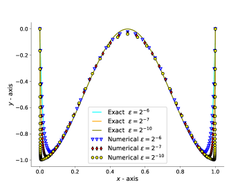
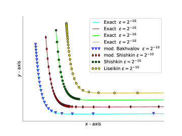
Figure 1: Exact and numerical solutions (left), layer near $x=0$ (right)–the difference scheme (15)

	$2^{-3}$		$2^{-5}$		$2^{-10}$		$2^{-20}$		$2^{-30}$		$2^{-40}$
$N$	$E_{n}$	Ord	$E_{n}$	Ord	$E_{n}$	Ord	$E_{n}$	Ord	$E_{n}$	Ord
$2^{4}$	6.590e-2	3.02	1.469e-1	1.83	1.678e-1	2.50	1.706e-1	2.48	1.706e-1	2.48	1.706e-1	2.48
$2^{5}$	1.593e-2	2.87	6.209e-2	2.74	5.172e-2	2.26	5.305e-2	2.31	5.305e-2	2.31	5.305e-e	2.31
$2^{6}$	3.670e-3	2.75	1.530e-2	2.86	1.627e-2	1.98	1.626e-2	1.99	1.626e-2	1.99	1.626e-2	1.99
$2^{7}$	8.325e-4	2.66	3.262e-3	2.76	5.576e-3	1.98	5.575e-3	1.98	5.575e-3	1.98	5.576e-2	1.98
$2^{8}$	1.869e-4	2.61	6.934e-4	2.65	1.836e-3	2.00	1.836e-3	2.00	1.836e-3	2.00	1.836e-3	2.00
$2^{9}$	4.153e-5	2.57	1.505e-4	2.55	5.820e-4	2.00	5.819e-4	2.00	5.819e-4	2.00	5.819e-4	2.00
$2^{10}$	9.126e-6	2.55	3.348e-5	2.46	1.797e-4	2.00	1.797e-4	2.00	1.797e-4	2.00	1.797e.4	2.00
$2^{11}$	1.981e-6	2.53	7.659e-6	2.37	5.438e-5	2.00	5.438e-5	2.00	5.438e-5	2.00	5.438e-5	2.00
$2^{12}$	4.249e-7	-	1.815e-6	-	1.618e-5	-	1.618e-5	-	1.618e-5	-	1.618e-5	-
						mesh (6)
$2^{4}$	2.349e-1	2.68	3.860e-1	1.72	4.453e-1	1.45	4.339e-1	1.42	4.533e-1	1.42	4.533e-1	1.42
$2^{5}$	6.662e-2	3.00	1.718e-1	2.37	2.242e-1	1.92	2.317e-1	1.89	2.317e-1	1.89	2.317e-1	1.89
$2^{6}$	1.434e-2	3.00	5.098e-2	2.68	8.388e-2	2.20	8.802e-2	2.18	8.802e-2	2.18	8.802e-2	2.18
$2^{7}$	2.840e-3	2.96	1.961e-2	2.65	2.555e-2	2.32	2.717e-2	2.30	2.718e-2	2.30	2.718e-2	2.30
$2^{8}$	5.407e-4	2.94	2.714e-3	2.65	6.946e-3	2.36	7.486e-3	2.33	7.487e-3	2.33	7.487e-3	2.33
$2^{9}$	9.946e-5	2.94	6.214e-4	2.50	1.782e-3	2.39	1.955e-3	2.32	1.955e-3	2.32	1.955e-3	2.32
$2^{10}$	1.765e-5	2.94	1.425e-4	2.46	4.362e-4	2.49	4.987e-4	2.30	4.988e-4	2.30	4.988e-4	2.30
$2^{11}$	3.033e-6	2.93	3.263e-5	2.43	9.826e-5	2.53	1.258e-4	2.27	1.259e-4	2.27	1.259e-4	2.27
$2^{12}$	5.129e-7	-	7.446e-6	-	2.111e-5	-	3.161e-5	-	3.162e-5	-	3.162e-5	-
						mesh (8)
$2^{4}$	1.759e-2	2.00	4.723e-2	1.94	8.772e-2	1.88	1.273e-1	1.80	1.277e-1	1.80	1.277e-1	1.80
$2^{5}$	4.440e-3	2.00	1.226e-2	2.02	2.367e-2	1.97	3.652e-2	1.95	3.666e-2	1.94	3.666e-2	1.94
$2^{6}$	1.102e-3	2.00	3.010e-3	1.97	6.023e-3	1.89	9.479e-3	1.99	9.514e-3	1.99	9.515e-3	1.99
$2^{7}$	2.757e-4	2.00	7.696e-4	2.00	1.623e-3	1.65	2.392e-3	2.00	2.401e-3	2.00	2.401e-3	2.00
$2^{8}$	6.894e-5	2.00	1.923e-4	2.00	5.140e-4	1.90	5.995e-4	2.00	6.018e-4	2.00	6.019e-4	2.00
$2^{9}$	1.723e-5	2.00	4.807e-5	2.00	1.372e-4	2.07	1.499e-4	2.00	1.505e-4	2.00	1.505e-5	2.00
$2^{10}$	4.309e-6	2.00	1.201e-5	2.00	3.258e-5	2.01	3.750e-5	2.00	3.764e-5	2.00	3.764e-5	2.00
$2^{11}$	1.077e-6	2.00	3.004e-6	2.00	8.114e-6	2.03	9.375e-6	2.00	9.411e-6	2.00	9.412e-6	2.00
$2^{12}$	2.693e-7	-	7.511e-7	-	1.985e-6	-	2.343e-6	-	2.352e-6	-	2.353e-6	-
						mesh (10)
$2^{4}$	6.113e-2	1.98	1.231e-1	1.96	1.859e-1	1.65	2.014e-1	1.63	2.027e-1	1.63	2.088e-1	1.63
$2^{5}$	1.546e-2	1.99	3.151e-2	2.09	5.895e-2	1.86	6.497e-2	1.85	6.548e-2	1.85	6.553e-2	1.85
$2^{6}$	3.869e-3	1.99	7.395e-3	2.04	1.627e-2	1.94	1.795e-2	1.94	1.810e-2	1.93	1.811e-2	1.93
$2^{7}$	9.675e-4	2.00	1.792e-3	2.01	4.192e-3	1.99	4.678e-3	1.97	4.719e-3	1.97	4.723e-3	1.97
$2^{8}$	2.418e-4	2.00	4.439e-4	2.00	1.052e-3	2.06	1.191e-3	1.98	1.201e-3	1.98	1.202e-3	1.98
$2^{9}$	6.046e-5	2.00	1.107e-4	2.00	2.517e-4	2.18	3.004e-4	1.99	3.030e-4	1.00	3.033e-4	1.99
$2^{10}$	1.511e-5	2.00	2.766e-5	2.00	5.531e-5	2.18	7.542e-5	2.00	7.608e-5	2.00	7.614e-5	2.00
$2^{11}$	3.779e-6	2.00	6.915e-6	2.00	1.219e-5	2.07	1.889e-5	2.00	1.905e-5	2.00	1.907e-5	2.00
$2^{12}$	9.448e-7	-	1.728e-6	-	2.887e-6	-	4.728e-6	-	4.769e-6	-	4.773e-6	-
						mesh (11)

Table 1: Results for difference scheme (15)

7 Conclusion

In this paper we give a discretization of a semilinear reaction–diffusion one–dimensional boundary–value problem. The difference scheme is constructed, the $\varepsilon$–uniform convergence of the order 2 on modified Shishkin mesh is shown. Similar results were obtained in one of the previous papers of the first author. But in that previous paper, the approximation of the function $\psi,$ which appears in the integrals, is very clumsily chosen. This made the analysis unnecessarily difficult. In this paper we have chosen a simplier approximation, which caused a simplier analysis. Another difficulty from the mentioned previous paper we didn’t overcome, here we used in our analysis the modified Shishkin mesh too, introduced by Vulanović. It is remain a task for some future paper to replace the modified Shishkin mesh by the Shishkin mesh. In the numerical experiments except the modified Shishkin mesh we used the Shishkin, the modified Bakhvalov, and the Liseikin mesh. All the meshes gave the expected results.

References

- [1] I.. Boglaev “Approximate solution of a non-linear boundary value problem with a small parameter for the highest-order differential” In Russian In Zh. Vychisl. Mat. i Mat. Fiz. 24.11, 1984, pp. 1649–1656 DOI: 10.1016/0041-5553(84)90005-3
- [2] E. Duvnjaković and S. Karasuljić “Difference Scheme for Semilinear Reaction-Diffusion Problem on a Mesh of Bakhvalov Type” In Mathematica Balkanica 25, Fasc. 5, 2011, pp. 499–504 URL: http://www.mathbalkanica.info/toc/siteCONT25-5.pdf
- [3] E. Duvnjaković and S. Karasuljić “Uniformly Convergente Difference Scheme for Semilinear Reaction-Diffusion Problem” In Conference on Appllied and Scietific Computing, Trogir, Croatia, 2011, pp. 25 URL: http://applmath11.math.hr/abs_book.pd
- [4] E. Duvnjaković and S. Karasuljić “Uniformly Convergente Difference Scheme for Semilinear Reaction-Diffusion Problem” In SEE Doctoral Year Evaluation Workshop, Skopje, Macedonia, 2011 URL: http://users.sch.gr/alexiouth/index.php/workshops/evaluation-ws
- [5] E. Duvnjaković and S. Karasuljić “Class of Difference Scheme for Semilinear Reaction-Diffusion Problem on Shishkin Mesh” In MASSEE International Congress on Mathematics - MICOM 2012, Sarajevo, Bosnia and Herzegovina, 2012
- [6] E. Duvnjaković and S. Karasuljić “Collocation Spline Methods for Semilinear Reaction-Diffusion Problem on Shishkin Mesh” In IECMSA-2013, Second International Eurasian Conference on Mathematical Sciences and Applications, Sarajevo, Bosnia and Herzegovina, 2013
- [7] E. Duvnjaković, S. Karasuljić and N. Okičić “Difference Scheme for Semilinear Reaction-Diffusion Problem” In 14th International Research/Expert Conference Trends in the Development of Machinery and Associated Technology TMT 2010, 7. Mediterranean Cruise, 2010, pp. 793–796 URL: http://www.tmt.unze.ba/zbornik/TMT2010/199-TMT10-138.pdf
- [8] E. Duvnjaković, S. Karasuljić and N. Okičić “Difference Scheme for Semilinear Reaction-Diffusion Problem” In 14th International Research/Expert Conference Trends in the Development of Machinery and Associated Technology TMT 2010, 7. Mediterranean Cruise, 2010, pp. 793–796 URL: http://www.tmt.unze.ba/zbornik/TMT2010/199-TMT10-138.pdf
- [9] E. Duvnjaković, S. Karasuljić, V. Pašić and H. Zarin “A uniformly convergent difference scheme on a modified Shishkin mesh for the singularly perturbed reaction-diffusion boundary value problem” In Journal of Modern Methods in Numerical Mathematics 6.1, 2015, pp. 28–43 DOI: 10.20454/jmmnm.2015.971
- [10] D. Herceg “Uniform fourth order difference scheme for a singular perturbation problem” In Numer. Math. 56.7 Springer-Verlag, 1989, pp. 675–693 DOI: 10.1007/BF01405196
- [11] D. Herceg and Dj. Herceg “On a fourth-order finite difference method for nonlinear two-point boundary value problems” In Novi Sad J. Math 33.2, 2003, pp. 173–180 URL: http://www.dmi.uns.ac.rs/nsjom/Papers/33_2/nsjom_33_2_173_180.pdf
- [12] D. Herceg and M. Miloradović “On numerical solution of semilinear singular perturbation problems by using the Hermite scheme on a new Bakhvalov-type mesh” In Novi Sad J. Math 33.1, 2003, pp. 145–162 URL: http://www.dmi.uns.ac.rs/nsjom/Papers/33_1/nsjom_33_1_145_162.pdf
- [13] D. Herceg and K. Surla “Solving a nonlocal singularly perturbed problem by spline in tension” In Review of research Faculty of Sciences-University of Novi Sad Vol.21, No.2, 1991, pp. 119–132 URL: http://www.dmi.uns.ac.rs/nsjom/Papers/21_2/NSJOM_21_2_119_132.pdf
- [14] S. Karasuljić “Construction of the Difference Scheme for Semilinear Reaction-Diffusion Problem on a Bakhvalov Type Mesh” In The Eighth Bosnian-Herzegovinian Mathematical Conference, Sarajevo, BiH, 2015
- [15] S. Karasuljić and E. Duvnjaković “Difference Scheme for Semilinear Reaction-Diffusion Problem on Layer–adapted Mesh” In The Seventh Bosnian-Herzegovinian Mathematical Conference, Sarajevo, BiH, 2012 URL: http://www.anubih.ba/Journals/vol.8,no-2,y12/16matskup7.pdf
- [16] S. Karasuljić, E. Duvnjaković and E. Memić “Uniformly Convergent Difference Scheme for a Semilinear Reaction-Diffusion Problem on a Shishkin Mesh” In Advances in Mathematics: Scientific Journal 7.1, 2018, pp. 23–38 URL: http://research-publication.com/wp-content/uploads/2019/03/AMSJ-2018-N1-4.pdf
- [17] S. Karasuljić, E. Duvnjaković, V. Pašić and E. Baraković “Construction of a global solution for the one dimensional singularly–perturbed boundary value problem” In Journal of Modern Methods in Numerical Mathematics 8.1–2, 2017, pp. 52–65 DOI: 10.20454/jmmnm.2017.1275
- [18] S. Karasuljić, E. Duvnjaković and H. Zarin “A uniformly convergent difference scheme on a Shishkin type mesh for the 2D singular perturbation boundary value problem” Submitted, 2015
- [19] S. Karasuljić, E. Duvnjaković and H. Zarin “Uniformly convergent difference scheme for a semilinear reaction-diffusion problem” In Advances in Mathematics: Scientific Journal 4.2, 2015, pp. 139–159 URL: http://research-publication.com/wp-content/uploads/2019/03/AMSJ-2015-N2-6.pdf
- [20] S. Karasuljić, E. Duvnjaković and H. Zarin “A uniformly convergent difference scheme on a modified Bakhvalov mesh for the singular perturbation boundary value problem” Submitted, 2018
- [21] S. Karasuljić and S. Halilović “Matematika 1” Off-set Tuzla, 2021
- [22] S. Karasuljić and H. Ljevaković “On construction of a global numerical solution for a semilinear singularly-perturbed reaction diffusion boundary value problem” In Mat. bilten 44.2, 2020, pp. 131–148 DOI: 10.37560/matbil2020131k
- [23] S. Karasuljić, H. Zarin and E. Duvnjaković “A class of difference schemes uniformly convergent on a modified Bakhvalov mesh” In Journal of Modern Methods in Numerical Mathematics 10.1-2 ModernScience Publishers, 2019, pp. 16–35 DOI: 10.20454/jmmnm.2019.1513
- [24] N. Kopteva “Maximum norm error analysis of a 2d singularly perturbed semilinear reaction-diffusion problem” In Mathematics of Computation 76.258 Washington, DC: National Academy of Sciences-National Research Council,[1960?-, 2007, pp. 631–646 DOI: 10.1090/S0025-5718-06-01938-7
- [25] N. Kopteva and T. Linß “Uniform second-order pointwise convergence of a central difference approximation for a quasilinear convection-diffusion problem” In J. Comput. Appl. Math. 137.2 Elsevier, 2001, pp. 257–267 DOI: 10.1016/S0377-0427(01)00353-3
- [26] N. Kopteva, M. Pickett and H. Purtill “A robust overlapping Schwarz method for a singularly perturbed semilinear reaction-diffusion problem with multiple solutions” In Int. J. Numer. Anal. Model 6, 2009, pp. 680–695 URL: http://www.global-sci.org/ijnam/readabs.php?vol=6&no=4&doc=680&year=2009&ppage=695
- [27] N. Kopteva and M. Stynes “A robust adaptive method for a quasi-linear one-dimensional convection-diffusion problem” In SIAM Journal on Numerical Analysis 39.4 SIAM, 2001, pp. 1446–1467 DOI: 10.1137/S003614290138471X
- [28] N. Kopteva and M. Stynes “Numerical analysis of a singularly perturbed nonlinear reaction–diffusion problem with multiple solutions” In Appl. Numer. Math. 51.2 Elsevier, 2004, pp. 273–288 DOI: 10.1016/j.apnum.2004.07.001
- [29] T. Linß, G. Radojev and H. Zarin “Approximation of singularly perturbed reaction-diffusion problems by quadratic -splines” In Numerical Algorithms 61.1 Springer US, 2012, pp. 35–55 DOI: 10.1007/s11075-011-9529-7
- [30] T. Linß, H.G. Roos and R. Vulanović “Uniform pointwise convergence on Shishkin-type meshes for quasi-linear convection-diffusion problems” In SIAM J. Numer. Anal. 38.3 SIAM, 2000, pp. 897–912 DOI: 10.1137/S0036142999355957
- [31] V.. Liseikin “Grid Generation for Problems with Boundary and Interior Layers” Novosibirsk State University, Novosibirsk, 2018
- [32] V.. Liseikin, S. Karasuljic, A.. Mukhortov and V.. Paasonen “On a Comprehensive Grid for Solving Problems Having Exponential or Power-of-First-Type Layers” In Lecture Notes in Computational Science and Engineering Springer International Publishing, 2021, pp. 227–240 DOI: 10.1007/978-3-030-76798-3_14
- [33] V.. Liseikin and S. Karasuljić “Numerical analysis of grid–clustering rules for problems with power of the first type boundary layers” In Computational Technologies 25.1, 2020, pp. 49–66 DOI: 10.25743/ICT.2020.25.1.004
- [34] V.D. Liseikin, Samir Karasuljić and V.I. Paasonen “Numerical Grids and High-Order Schemes for Problems with Boundary and Interior Layers” Novosibirsk State University, 2021
- [35] V.D. Liseikin and Poaasonen “Compact Difference Schemes and Layer Resolving Grids for Numerical Modeling of Problems with Boundary and Interior Layers” In Numer. Analys. Appl. 12, 2019, pp. 37–50 DOI: 10.1134/S199542391901004X
- [36] V.D. Liseikin et al. “On Rules for Grid Clustering in the Zones of Boundary and Interior Layers” In Mathematics and its Applications. International Conference in honor of the 90th birthday of Sergei K. Godunov, 2019 Novosibirsk, Russia
- [37] Vladimir Liseikin, Samir Karasuljić, Aleksandr Mukhortov and Viktor Paasonen “On a comprehensive grid for solving problems having exponential or power–of–first–type layers” In NUMGRID 2020, Moscow, Russia, 2020 Dorodnicyn Computing Center FRC CSC RAS
- [38] J. Lorenz “Stability and monotonicity properties of stiff quasilinear boundary problems” MR 85e:34046 In Zb.rad. Prir. Mat. Fak. Univ. Novom Sadu, Ser. Mat. 12, 1982, pp. 151–176 URL: http://www.emis.de/journals/NSJOM/Papers/12/NSJOM_12_151_175.pdf
- [39] J.. Ortega and W.. Rheinboldt “Iterative Solution of Nonlinear Equations in Several Variables” SIAM, Philadelphia, USA, 2000
- [40] G.. Shishkin “Grid approximation of singularly perturbed parabolic equations with internal layers” In Sov. J. Numer. Anal. M.Russian Journal of Numerical Analysis and Mathematical Modelling 3.5, 1988, pp. 393–408 DOI: 10.1515/rnam.1988.3.5.393
- [41] M. Stynes and N. Kopteva “Numerical analysis of singularly perturbed nonlinear reaction-diffusion problems with multiple solutions” In Computers and Mathematics with Applications 51.5 Elsevier, 2006, pp. 857–864 DOI: 10.1016/j.camwa.2006.03.013
- [42] G. Sun and M. Stynes “A uniformly convergent method for a singularly perturbed semilinear reaction-diffusion problem with multiple solutions” In Math. Comput. 65.215, 1996, pp. 1085–1109 URL: http://www.jstor.org/stable/2153793
- [43] K. Surla and Z. Uzelac “On Stability of Spline Difference Scheme for Reaction-Diffusion Time-Dependent Singularly Perturbed Problem” In Novi Sad J. Math. 33.2, 2003, pp. 89–94 URL: http://www.dmi.uns.ac.rs/nsjom/Papers/33_2/nsjom_33_2_089_094.pdf
- [44] R. Vulanović “On a Numerical Solution of a Type of Singularly Perturbed Boundary Value Problem by Using a Special Discretization Mesh” In Novi Sad J. Math. 13, 1983, pp. 187–201 URL: http://www.dmi.uns.ac.rs/nsjom/Papers/13/NSJOM_13_187_201.pdf
- [45] R. Vulanović “On a numerical solution of a type of singularly perturbed boundary value problem by using a special discretization mesh” In Univ. u Novom Sadu Zb. Rad, Prirod-Mat. Fak. Ser. Mat 13, 1983, pp. 187–201 URL: http://www.dmi.pmf.uns.ac.rs/nsjom/Papers/13/NSJOM_13_187_201.pdf
- [46] R. Vulanović “Mesh generation methods for numerical solution of quasilinear singular perturbation problems” In Univ. u Novom Sadu Zb. Rad, Prirod-Mat. Fak. Ser. Mat 19.2, 1989, pp. 171–193 URL: http://www.emis.ams.org/journals/NSJOM/Papers/19_2/NSJOM_19_2_171_193.pdf
- [47] R. Vulanović “A second order numerical method for non-linear singular perturbation problems without turning points” In USSR Comp. Math. Math+. 31.4, 1991, pp. 522–532
- [48] R. Vulanović “On numerical solution of semilinear singular perturbation problems by using the Hermite scheme” In Univ. u Novom Sadu Zb. Rad, Prirod-Mat. Fak. Ser. Mat 23.2, 1993, pp. 363–379 URL: http://www.dmi.uns.ac.rs/nsjom/Papers/23_2/NSJOM_23_2_363_379.pdf
- [49] R. Vulanović “A Higher-order Scheme for Quasilinear Boundary Value Problems with Two Small Parameters” In Computing 67.4 Springer-Verlag New York, Inc., 2001, pp. 287–303 DOI: 10.1007/s006070170002
- [50] R. Vulanović “An almost sixth-order finite-difference method for semilinear singular perturbation problems” In Computational methods in applied mathematics 4.3, 2004, pp. 368–383 DOI: 10.2478/cmam-2004-0020