Analysis of Augmentations for Contrastive ECG Representation Learning

Abstract

This paper systematically investigates the effectiveness of various augmentations for contrastive self-supervised learning of electrocardiogram (ECG) signals and identifies the best parameters. The baseline of our proposed self-supervised framework consists of two main parts: the contrastive learning and the downstream task. In the first stage, we train an encoder using a number of augmentations to extract generalizable ECG signal representations. We then freeze the encoder and finetune a few linear layers with different amounts of labelled data for downstream arrhythmia detection. We then experiment with various augmentations techniques and explore a range of parameters. Our experiments are done on PTB-XL, a large and publicly available 12-lead ECG dataset. The results show that applying augmentations in a specific range of complexities works better for self-supervised contrastive learning. For instance, when adding Gaussian noise, a sigma in the range of 0.1 to 0.2 achieves better results, while poor training occurs when the added noise is too small or too large (outside of the specified range). A similar trend is observed with other augmentations, demonstrating the importance of selecting the optimum level of difficulty for the added augmentations, as augmentations that are too simple will not result in effective training, while augmentations that are too difficult will also prevent the model from effective learning of generalized representations. Our work can influence future research on self-supervised contrastive learning on bio-signals and aid in selecting optimum parameters for different augmentations.

I Introduction

An electrocardiogram (ECG) is a non-invasive and effective tool for measuring the electrical activity of the heart [1]. ECG signals convey valuable information about the functionality and condition of the heart, including heart rate, blood pressure, and heart diseases. In recent years, deep learning solutions have been used to create effective and robust ECG-based diagnostics and therapeutic tools. Examples include the use of deep neural networks for detection of cardiovascular diseases such as different types of Arrhythmia [2, 3, 4, 5, 6, 7].

Supervised deep learning methods often require large amounts of labelled data to perform optimally. However, this is not always the case for many physiological data such as ECG recordings. The tedious nature of the labeling process and the required highly specialized domain knowledge makes the task extremely costly. In addition, some conditions such as long QT [8] are relatively rare among the population, making the collection of such data even more difficult. Also, in many cases, the fluidity of medical definitions leads to high inter-observer variability and a lack of a gold standard (for instance the definition of type 3 long QT [9, 10]). In such cases, classical supervised deep learning methods may counter challenges and eventually lead to sub-optimal performance.

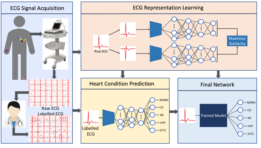
Figure 1: An overview of a self-supervised ECG representation learning system for arrhythmia detection.

Self-supervised learning is a feature learning technique for overcoming the challenges related to the scarcity of ‘labelled’ data [11, 12, 13, 14]. This relies on the generation of pseudo-labels from various augmentations for data during training instead of using pre-annotated data with ground truth labels. Thanks to their ability to generate a variety of different augmentations with varying degrees of difficulty, self-supervised learning often results in learning more generalized representations [15], making it highly accurate and robust toward different variations in the training data. Contrastive learning is a form of self-supervision in which a data sample is augmented to create positive pairs, while other samples are considered negative pairs [16, 17, 18]. These positive and negative pairs are then used to train a Siamese style network and learn representations where the positive pairs maintain close proximity while the negative pairs are situated far apart in the feature space. Variations of contrastive methods in which negative pairs are no longer required for training have also been recently proposed [19]. Prior works have shown the the choice of ‘type’ and ‘intensity’ of augmentations used for contrastive self-supervised learning can have a considerable impact on the model performance [20, 21]. Thus, this paradigm poses a new set of challenges in that the optimum parameters regarding the augmentations need to be carefully designed and incorporated into the self-supervised training pipeline.

In this paper we design and implement a contrastive self-supervised framework for ECG-based arrhythmia detection (see Figure 1). First we contrastively train a deep convolutional neural network (CNN) encoder to learn representations from input ECG signals obtained from the PTB-XL dataset [22]. We then freeze the encoder and finetune a few linear layers with different amounts of labelled samples for downstream arrhythmia classification. Our goal is to provide a comprehensive analysis of the impact of different augmentations and their parameters towards contrastive ECG learning. To this end, we experiment with 7 different commonly used augmentations and systematically study their impact across different intensity parameters. We identify that the addition of Gaussian noise, permutation, and time warping yield strong results when specific ranges of parameters are used. We also experiment with different encoder architectures to ensure that our findings generalize well across different CNN encoders.

II Related Work

II-A Supervised ECG Learning

There has been extensive research on ECG classification for different tasks. Researchers have used intrinsic features of ECG in classical machine learning techniques for ECG classification [23, 24, 25]. In recent years, with the evolution of deep learning models and the creation of relatively large ECG datasets, ECG classification using deep learning models has become prominent [26, 27, 28]. In this section, we provide a summary of some key works in the field of ECG classification, ranging from past classical machine learning-based algorithms to more recent deep learning-based methods.

In classical machine learning approaches, researchers largely relied on important ECG features. These features include the PQRST complex and their time intervals, such as the RR interval [29, 30], QRS duration [25, 31], QT interval [23, 32, 24], as well as statistical and morphological features [33, 34, 35, 36, 37]. A comprehensive survey in this domain can be found in [38].

When it comes to deep learning solutions, we first present the prior work on ECG representation learning using fully supervised approaches based on two main categories of neural networks, namely convolutional neural networks (CNNs) and recurrent neural networks (RNNs). In [39], an ECG heartbeat classifier using a 1D CNN model was proposed. This classifier achieved strong performance for a five class arrhythmia classification. In [40] a Generic Convolutional Neural Network was first trained on a large number of ECG signals. Then, to learn distinctive features of each patient’s ECG, the network was finetuned on the patient’s ECG signals individually. In [41], an accurate and sensitive myocardial infarction (MI) detector was proposed. A CNN model trained on 12-lead ECG signals was used for this purpose. In [42], a 2D CNN was proposed for predicting arrhythmia using transformed ECG signals to 2D grayscale images. In [43] a subject-specific CNN was proposed for arrhythmia classification from ECG signals. The signals were transformed into a 2D matrix which preserved their temporal and morphological features. The model was trained on the most representative heartbeats for improving the performance. In [44], two ECG classifiers were presented using 1D and 2D CNN models. In this work, the 2D CNN model trained on ECG signals transformed to 2D images showed better results than the 1D CNN.

In [45], an ECG classifier was proposed in three phases, including an eigenvector feature extractor, a feature selector, and an RNN, which was trained on the extracted features. In [27], a four-class ECG classifier was presented using RNNs. The ECG signal’s features were first extracted, and then the classification was made using selected features as inputs to the RNN model. In [26], a patient-specific RNN based ECG signal classifier was presented. Some morphology features of ECG signals were fed into RNN for better performance. In [46], various RNN-based architectures were evaluated for ECG classification, and authentication with no need for ECG extracted features. In [47], a bidirectional gated RNN (BGRU) was introduced for ECG signal identification. The benefit of their proposed method was the network’s ability to see both the past and future signal time steps simultaneously, which allowed for a better understanding of the ECG representations. Lastly in [28], an ECG feature extractor was proposed named Global RNN (GRNN). Every input ECG signal feature was extracted, and the most informative samples were selected by the optimization mechanism and set as the model’s training data for better generalizability.

II-B Self-supervised ECG Representation Learning

With the recent progress in self-supervised learning in areas such as computer vision [17] and natural language processing [48], a number of recent works have utilized such methods for ECG representation learning. In what follows, we briefly present some prior work in this area. In [49, 50], self-supervised ECG-based emotion recognition was proposed to improve the network’s performance in comparison to fully supervised learning. In this work, spatiotemporal ECG representations were learned by applying various transformations to unlabelled ECG signals, followed by predicting the applied transformation. Next, the downstream task was performed by freezing the pre-trained encoder component of the model and training a few dense layers with labelled data. In [51], a contrastive self-supervised learning approach was proposed for bio-signals. They tackled the inter-subject adverse effects on learning by presenting subject-aware optimization using a subject distinctive contrastive loss and adversarial training.

In [52], a framework called CLOCS was proposed, in which a patient-specific contrastive learning method was able to achieve state-of-the-art results by learning the spatiotemporal representations of ECG signals. The method also benefited from the physiological features of ECG signals, namely temporal and spatial invariance to produce additional positive pairs from each patient signal. A model called TS-TCC was proposed in [53] which learned time-series data representations by creating two views of each sample by applying a strong and weak data augmentation, and then learning robust temporal features by applying a cross-view prediction task. In another method called 3KG proposed in [54], ECG representations were learned in a contrastive manner using physiological characteristics of ECG signals. 12-lead signals were transformed to a 3D space followed by application of augmentations in that space. The method was evaluated by finetuning on different heart diseases and produced strong results. Lastly, an approach called CLECG which was proposed in [55] presented a contrastive self-supervised learning framework for ECG signals. The method utilized random cropping and wavelet transformations for contrastive learning augmentations.

In the end, we conclude from our review that self-supervised methods for ECG representation learning provide very promising results in comparison to fully supervised approaches. Nonetheless, the difficulty in labeling large amounts of data by experts poses open challenges in the area, and thus self-supervised solutions including contrastive learning are projected to further dominate the field. However, while the choice of encoder and classifier architectures in self-supervised frameworks is generally not too critical, the choice of the type and intensity of pretext or contrastive augmentations plays a critical role in ECG representation learning. This motivates our work presented in this paper where we provide a detailed analysis of different augmentations for ECG representation learning.

III Method

In this section, we first explain our self-supervised contrastive framework shown in Figure 2. We then describe each of the augmentations that are applied to the ECG signals. Lastly we present the architectural details of different components of the pipeline.

III-A Self-Supervised Contrastive Framework for ECG Representation Learning

Assume our input ECG signal as $x\in\mathbb{R}^{D\times L}$, where $D$ is the number of ECG leads, and $L$ is the length of each signal. In the first step, we apply an augmentation on $x$ and obtain the augmented sample $\tilde{x}$. The details of these augmentations will be explained in the next sub-section. Accordingly, we can assume $\tilde{x}$ as another view of $x$, and therefore, $x$ and $\tilde{x}$ are called positive pairs. Also, $x$ and $\tilde{x}$ make negative pairs with other input data and their respective augmentations. For better understanding, consider two different input ECG signals as $x_{a}$ and $x_{b}$, and their augmentations $\tilde{x}_{a}$ and $\tilde{x}_{b}$. In this example, the positive pairs are ($x_{a}$, $\tilde{x}_{a}$) and ($x_{b}$, $\tilde{x}_{b}$), while the negative pairs are ($x_{a}$, $x_{b}$), ($x_{a}$, $\tilde{x}_{b}$), and ($x_{b}$, $\tilde{x}_{a}$).

Next, input signal $x_{i}$ and its augmented version $\tilde{x}_{i}$ are separately passed to our encoder model referred to as $E(.)$ through the two separate branches of our pipeline (see Figure 2), and result in $h_{i}$ and $\tilde{h}_{i}$. Next, $h_{i}$ and $\tilde{h}_{i}$ are passed through linear fully connected layers $G(.)$ for better characterization. The final outputs are $z_{i}$ and $\tilde{z}_{i}$, which are passed to the loss function for calculating the overall model contrastive loss. We use the loss presented in [16, 56] for the contrastive training stage of our framework. This loss function maximizes the agreement between different views of each sample, using the variations among different samples. The loss function is formulated as:

$$L_{contr}=-log(\frac{exp(sim(z_{i},\tilde{z}_{i})/\tau)}{\sum_{k=1}^{2N}\mathbbm{1}_{(i\neq k)}exp(sim(z_{i},z_{k})/\tau)}),$$ (1)

where $N$ is the batch size and $\tau$ is the temperature parameter. The $sim(z_{i},\tilde{z}_{i})$ function used in the loss formula is the cosine similarity with the formulation of:

$$sim(z_{i},\tilde{z}_{i})=\frac{z_{i}.\tilde{z}_{i}}{\parallel z_{i}\parallel\parallel\tilde{z}_{i}\parallel}.$$ (2)

Following some previous works [17, 54], in a batch of size $N$, only each sample and its augmented form are selected as positive pairs, while the other $2N-2$ samples are selected from negative pairs.

After contrastive training of the network, we freeze the weights of $E(.)$ and transfer them to another pipeline for the downstream task. In this step, $G(.)$ is no longer required and thus discarded. Please refer to Figure 2. In this phase, we use labelled samples $(x_{j},l_{j})$ where $x_{j}$ is the sample and $l_{j}$ is its label. $(x_{j},l_{j})$ is fed to the pretrained $E(.)$ followed by a few untrained fully connected layers $C(.)$. The goal of these layers is to perform the final classification and $c_{j}$ are the predicted classes. The network is then trained by supervised learning with Binary Cross-Entropy (BCE) loss. The formula for the BCE loss is as follows:

$$L_{BCE}=-\frac{1}{N}\sum_{i=1}^{N}[l_{i}\times log(c_{j})+(1-l_{j})\times log(1-c_{j})],$$ (3)

where $N$ is the total number of fine-tuning samples in each batch, $l_{j}$ is sample’s true label and $c_{j}$ is the model output for the $j^{th}$ class.

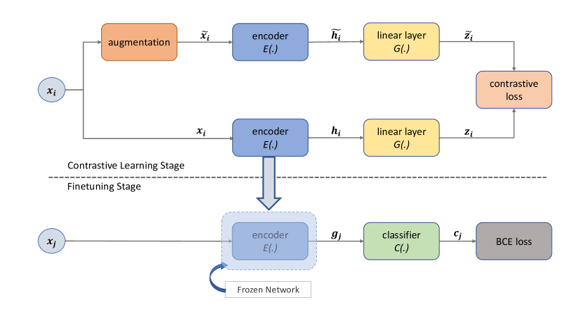
Figure 2: The contrastive framework used in our study.

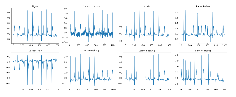
Figure 3: Different augmentations applied on a sample ECG segment.

III-B Augmentations

As observed and discussed earlier in Section 2, in self-supervised and contrastive approaches, the type and intensity of different augmentations used to learn ECG representations in the contrastive learning step can play a critical role in downstream classification. Here, to conduct a detailed and rigorous study on this aspect of our contrastive learning framework, we carefully select a large number of augmentations that have been shown in different literature to help with generalization in ECG learning. Some of these augmentations very closely resemble artifacts that can appear in the wild or even in the lab when acquiring ECG signals, and therefore their use in contrastive self-supervised learning can help the model extract effective and used representations and generalize to unseen data. For instance the addition of Gaussian noise can occur in various scenarios when recording ECG data. As another example, ECG can be scaled due to changes in sensor conductance that can occur naturally. As another example, ECG samples may also be dropped during collection. In addition to the impact of the type of augmentation, their intensities can also greatly impact the outcome. Prior works have shown that generally during self-supervised learning, when augmentations are very weak, poor representations are learned since the augmented signals are very similar to the input samples. On the other hand, it has been also shown that when augmentations are too strong, the augmented samples are so different from the original signals that the network does not learn useful and generalizable representations. As a result, we use eight different augmentation techniques in our framework and systematically cover a wide range for their respective parameters. The augmentation details are as follows.

III-B1 Noise

We add Gaussian noise $N(t)$ to the ECG signal $x(t)$. This is formulated as: $P(x)=\frac{1}{\sqrt{2\pi\sigma}}e^{-\frac{(x-\mu)^{2}}{2\sigma^{2}}}$, where $\mu$ is the mean value set to zero, and $\sigma$ is the standard deviation for our augmentations. The augmented ECG signal is computed by adding the noise signal to the ECG as $\tilde{x}(t)=x(t)+N(t)$.

III-B2 Scale

The input ECG is multiplied by a scaling factor $S$ to obtain $\tilde{x}(t)=S\times x(t)$.

III-B3 Permutation

In this augmentation, the ECG signal is divided into $m$ sub-sections, ${x_{1},x_{2},...,x_{m}}$. These sub-sections are then shuffled and concatenated together to make the augmented signal $\tilde{x}$.

III-B4 Vertical Flip

The input signal is flipped vertically across the time axis as $\tilde{x}(t)=-x(t)$.

III-B5 Horizontal Flip

To perform this augmentation, we modify $x(t)$ as $\tilde{x}(t)=x(-t+L)$ where $L>0$ is the length of $x(t)$.

III-B6 Zero Masking

For this augmentation, a masking factor $r$ is selected which determines the percentage of the original signal $x(t)$ that will be set to zero. Next, we randomly set $r\times L$ consecutive samples of $x(t)$ to zero to obtain $\tilde{x}(t)$.

III-B7 Time Warping

For this augmentation, we divide $x(t)$ into $m$ segments $x_{1}(t),\cdots,x_{m}(t)$ where $m$ is even. Next, we use time warping to stretch half of the segments (randomly selected) by $w\%$ while simultaneously squeezing the other half by the same factor. The segments are finally concatenated in the same order to obtain $\tilde{x}(t)$ where the final length of $\tilde{x}(t)$ remains unchanged as $L$.

Figure 3 illustrates an input ECG signal, as well as samples of each of the augmentations mentioned above. We can observe that each augmentation alters the spatiotemporal properties of the signal in a unique way, overall resulting in a wider distribution of shapes and characteristics, which can lead to more generalized learning.

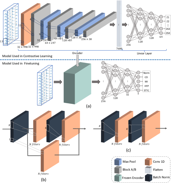
Figure 4: The architecture details of (a) encoder and linear layers for contrastive training and fine-tuning, (b) the block architecture of Encoder A, and (c) the block architecture of Encoder B.

III-C Model Details

As discussed earlier in Section 3.A, our framework uses a deep encoder, $E$, for extracting ECG features from raw data. In order to explore the flexibility and generalizability of our proposed model, we use two different CNN architectures for $E$. The first model is based on residual network adopted from [51], which has shown great performance in bio-signal classification. Henceforth, we refer to this network as Encoder A. As shown in Figure 4(a) and (b), this encoder contains one 1D convolutional layer, four residual blocks (ResBlocks), three max-pooling layers, and a Flatten layer. Each ResBlock consists of two 1D convolutional layers with ELU activation function, two batch normalizations, and a 1D convolutional layer with a residual connection. The numbers in the convolutional blocks of Figure 4 represent the number of input channels, output channels, and kernel sizes respectively.

A flatten layer as the final step of the encoder, which outputs a final feature vector with the size of $1\times 7680$. The second encoder, Encoder B, consists of layers similar to Encoder A, except for the residual connections inside the convolutional blocks. The details can be seen in Figure 4(a) and (c).

Following the encoder, we use four feed-forward linear layers with ReLU activation functions. The numbers in the linear layers in Figure 4 (a) represent the input and output sizes respectively.

In the end, as described earlier in Section 3.A, after training the contrastive model, the encoder is frozen and a classification model is added and fine-tuned. This classifier consists of four fully connected layers with ReLU activation functions. The details of this stage of the model is presented in Figure 4(a).

TABLE I: The details of the augmentation parameters used for contrastive learning.

Augmentation Method	Min	Max	Data Points
Gaussian Noise ($\sigma$)	0.01	1	[0.01, 0.03, 0.05, 0.07, 0.1,
			0.15, 0.2, 0.25,0.4, 0.6, 0.9]
Scale ($S$)	0.1	3	[0.1, 0.3, 0.5, 0.8, 1.2,
			1.7, 2, 2.5, 3]
Permutation	2	20	[2, 4, 5, 8, 10, 20]
Horizontal Flip	–	–	–
Vertical Flip	–	–	–
Zero Mask ($r$)	10%	60%	[10%, 20%, 30%, 40%,
			50%, 60%]
Time warping	0.25	0.75	[2-(0.25, 0.5, 0.75),
			4-(0.25, 0.5, 0.75)]

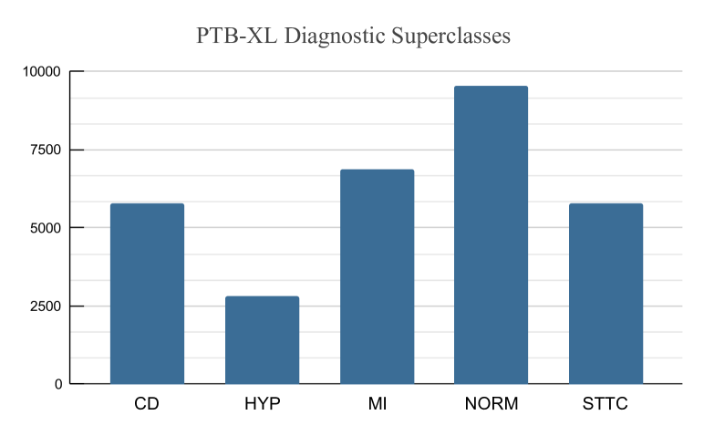
Figure 5: The distribution of classes in the PTB-XL dataset.

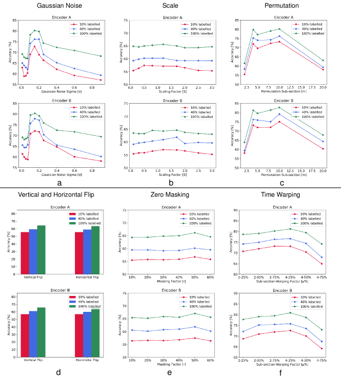
Figure 6: Accuracy of our contrastive self-supervised model for different augmentation parameters: (a) adding Gaussian noise, (b) scaling, (c) permutating, (d) vertical and horizontal flipping, (e) zero masking, and (f) time warping. Two encoders, A (with residual connections) and B (without residual connections), have been used in these experiments.

IV Experiments and Results

IV-A Dataset

We use a large publicly available dataset, PTB-XL [22]. This dataset consists of 21837 samples of 12-lead ECG from 18885 patients collected with Schiller AG devices. The dataset is categorized into five main classes, normal, myocardial infarction, conduction disturbance, ST/T changes, and hypertrophy. Figure 5 shows the distribution of these five classes in detail. The dataset is provided with two sampling frequencies, 100 and 500 Hz. In our work, we used signals with a frequency of $f_{s}$=100 Hz to reduce our computational requirements. The dimension of the ECG samples fed into our model is $12\times 1000$, corresponding to 1000 points that is 10 seconds long and 12-leads.

IV-B Training Details and Evaluation

PTB-XL dataset is initially separated into ten subsections, and by using these subsection, we split the dataset into two main subsections, 10% for testing the model’s performance, and 90% for contrastive training and finetuning. For evaluating the effects of the number of labelled data in finetuning the model, each model is finetuned three times using different amounts of training data, $\frac{1}{9}$, $\frac{4}{9}$ and $\frac{9}{9}$, henceforth approximated and referred to as 10%, 40%, and 100%.

We use Adam optimizer [57] with a learning rate of $5\times 10^{-4}$ and weight decay of $1\times 10^{-3}$ to train the contrastive framework. The contrastive stage is trained for 50 epochs with a batch size of 128. In the downstream phase, the added linear layers are trained for 200 epochs using Stochastic Gradient Descent (SGD) optimizer with a learning rate of 0.01. We use weighted accuracy to evaluate the performance of our model. The method is implemented using PyTorch and trained on NVIDIA GeForce GTX 1070 GPU.

IV-C Results

This section illustrates our experimental results on the PTB-XL dataset. As comprehensively described earlier in section 3.A, we apply seven different augmentations on ECG signals. For each augmentation, we use various parameters as shown in Table I. To examine the efficiency of Gaussian noise adding to ECG signal, we use Gaussian noise with zero mean and $\sigma$ in the range of $0.01-0.9$, with a step size of $0.05$. We use scale augmentation with a scaling factor of $0.1-3$ and a step size of $0.2$. The zero-masking augmentation is applied on the ECG signals with a range of $10\%-60\%$ and a step size of $10\%$. For permutation augmentation, a range of $2-20$ is selected with a step size of $2$. Two different variations are used for time warping, one where the signal is segmented into 2 pieces, while in the other, the signal is divided into 4 segments. We apply 3 different scaling factors for each variation, $25\%$, $50\%$, and $75\%$. We also flip the ECG signals both horizontally and vertically. The results for each of these augmentations are shown in Figure 6. We observe that as expected, different augmentations and different parameters result in varied accuracies. We further train the inference model (Figure 4 (a) finetuning) in a fully supervised manner with all the training labels available. As we dive into each augmentation result in detail in the following paragraphs, the fully supervised results shown in Figure 6 provide a valuable benchmark in understanding the impact of each augmentation. We should point out that while the performance of self-supervised learning is expectedly lower than the fully supervised counterpart in most cases, it is significantly less reliant on the labels during training as only the classifier portion is trained using the original labels.

In Figure 6 (top left) we observe that augmenting via Gaussian noise results in learning strong ECG representations in the range of $\sigma=$ $0.1$ to $0.25$, while outside of this range, performance drops. This is due to the fact that when $\sigma=[0.01-0.07]$, the augmentation is likely too weak, resulting in augmented ECG signals that are very similar to the original signals. The network therefore does not learn effectively. On the other hand, for $\sigma=[0.4-0.9]$, we hypothesize that the augmentation is too strong, and thus the augmented ECG signal looks very different from the original signal. Therefore, associating the two signals as the same sample becomes too difficult for the network, and thus learning does not take place effectively. Next, we observe that a similar trend is observed when different amounts of labels ($10\%$, $40\%$ and $100\%$) are used during finetuning. However, while the use of larger amounts of labelled data results in better overall performance, our model does not suffer considerably when the amount of labels are reduced by approximately $90\%$. Lastly, both Encoder A and Encoder B exhibit similar performances, which point to the generalizability of our approach.

Figure 6 (top middle) demonstrates that the scaling augmentation on ECG signals does not show overall promising results in comparison to the other applied augmentations. Nevertheless, the results slightly improve when scaling with the scaling factor of $S=[0.5-1.7]$. We believe that scaling does not show favourable results given that this augmentation is too simple, and does not apply sufficient spatiotemporal changes to the signal for the augmented samples to expand the learned distribution for better representation learning. We further observe that varying amounts of labelled data used for finetunig increases the performance by approaximately $10\%$, yet, the results are still not very strong and only a very weak trend can be seen with respect to the scaling factor. Moreover, the choice of the encoder does not considerable affect the performance, pointing to the fact that this augmentation, at least when used individually, is likely not very helpful towards self-supervised contrastive ECG learning.

We observe from Figure 6 (top right) that when the permutation augmentation is applied on ECG signals, using $2$ and $20$ sub-sections does not show promising results. We believe that using $2$ sub-sections will result in augmentations that are too simple to learn for the model, while using $20$ sub-sections becomes extensively challenging to learn. As mentioned earlier, each ECG sample is $10$ seconds long in our experiments. On average, the resting human heart rate is between $60$ and $100$ beats per minute [58], which means that our ECG samples are likely to have $6$ to $10$ heartbeats per sample. Therefore, when we divide these samples into 20 sub-sections and shuffle them randomly, it is likely that the resulting augmented sample does not resemble an ECG signal anymore, which is why the network is not able to learn ECG representations, and thus poor performance. Similar to the Noise augmentation which also proved to be effective, we observe that reduction of labelled data for finetuning, even by the significant amount of $90\%$, does not hurt the performance considerably. Moreover, the choice of encoder does not hugely impact the results. In the end, we conclude that by and large, this augmentation is effective for contrastive ECG learning.

The results shown in Figure 3 (bottom left) indicate that vertical and horizontal flip, on the other hand, are not effective augmentations. We hypothesize that the spatiotemporal properties of the resulting signals are different enough from the original samples that the network is unable to learn. The behaviour of the model when trained with these augmentations is similar to other augmentations in terms of the use of labelled samples or encoder. As seen in Figure 3 (bottom middle), also does not show promising results regardless of the choice of encoder or the amount of labelled data. We do observe a small peak in the accuracy with $L=50\%$, but overall, this augmentation does not seem to allow the network to learn effective ECG representations. Further details on the limitations of our experiment design in this regard and how to potentially improve the model to benefit from this augmentation is discussed below in the Limitations section.

Finally, Figure 3 (bottom right) presents the results of the time warping augmentation, which shows promising performance. We observe that when we divide the ECG signal into 2 segments and then apply time warping, the stronger squeeze and stretch factor achieves better results. However, when dividing the signal into 4 segments, the weaker squeeze and stretch factor shows better performance. We believe that for fewer ECG segments, i.e. 2, for the model to learn better representations, we need a stronger squeeze and stretch factor so that the augmented signal does not become too easy for the model to learn. Yet for more segments, the smaller squeeze and stretch factor works better since the augmentation is already not so simple and it is not reasonable to add even more complexity by using the stronger squeeze and stretch factor.

In the end, in order to obtain a high-level view of the augmentations in comparison to one another, Table II illustrates the best results obtained for each augmentation and for different amounts of labelled data used in finetuning. We also train both our models in a fully supervised manner to achieve a better understanding of the effectiveness of contrastive training. For the model with Encoder A we achieve an accuracy of $82.428$, and for the model with Encoder B, we get $84.876$ accuracy. From this analysis, we observe that adding Gaussian noise, permutation, and time warping show the best performances for contrastive ECG learning, while scaling, zero masking, and vertical/horizontal flipping show lower performances.

TABLE II: Comparison of the best accuracies achieved with Encoder A (residual) and Encoder B (non-residual) using different augmentations and finetuned with 10%, 40%, and 100% labelled data.

Augmentation	Labelled Data	Model A	Model B
	10%	68.91	72.13
Gaussian Noise	40%	76.17	77.87
	100%	80.17	80.31
	10%	57.41	57.04
Scale	40%	60.27	61.89
	100%	65.62	64.65
	10%	73.27	75.04
Permutation	40%	76.27	79.14
	100%	80.19	84.73
	10%	55.47	57.03
Vertical Flip	40%	59.28	60.16
	100%	64.45	65.83
	10%	55.66	56.98
Horizontal Flip	40%	58.94	58.03
	100%	64.50	65.94
	10%	56.77	57.51
Zero Masking	40%	60.14	61.86
	100%	66.14	67.05
	10%	73.13	72.54
Time Warping	40%	76.61	75.72
	100%	81.18	80.87

IV-D Limitations

Our study has a number of limitations which will be explored in future work. (i) One approach in expanding out work will be to explore smaller step sizes and larger ranges in our search for the optimum parameters for the augmentations. For instance, the zero-masking augmentation can be modified to allow for shorter zero-masked segments distributed throughout the ECG signal. (ii) Moreover, more advanced augmentations, for example those in the frequency domain, could be considered. (iii) To further explore the generalizability and practicality of our study, additional datasets as well as larger number of output classes will be trained and evaluated against. In particular, a study of augmentations that aid in classification of various types of arrhythmia will be conducted to allow for arrhythmia-specific findings. (iv) In this study, we explored each augmentation individually. Nonetheless, combinations of augmentations may exhibit different behaviors, which we will explore through forward/backward selection methodologies. (v) Lastly, additional variations of contrastive learning can be studied and explored for identifying the optimum set of augmentations.

V Conclusion

This paper highlights the significance of augmentation selection for ECG representation learning using contrastive self-supervised learning. Our experiments are done on the PTB-XL, a large and public arrhythmia-specified dataset. In our experiments, the primary model is first trained with unlabelled augmented data contrastively to learn ECG representations, followed by freezing the encoder and finetuning a few linear layers with different amounts of labeled data to conceive the final results. Our experiments demonstrate that particular augmentation techniques result in better and more generalizable learning of ECG representations with some augmentations such as vertical/horizontal flipping showing poor performance. Moreover, we find that the range of augmentation complexities plays an important role in the performance as augmentations that are too weak or too strong do not result in effective training. Our study uncovers optimum ranges of complexities for different augmentations such as noise addition, time warping, and permutation, which can be used by researchers in the area for effective self-supervised ECG representation learning.

References

- [1] “Electrocardiogram”, Johns Hopkins Medicine, 2021 [Online] URL: https://www.hopkinsmedicine.org/health/treatment-tests-and-therapies/electrocardiogram
- [2] Rasmus S. Andersen, Abdolrahman Peimankar and Sadasivan Puthusserypady “A deep learning approach for real-time detection of atrial fibrillation” In Expert Systems with Applications 115, 2019, pp. 465–473
- [3] Ali Isin and Selen Ozdalili “Cardiac arrhythmia detection using deep learning” In Procedia Computer Science 120, 2017, pp. 268–275
- [4] Giovanna Sannino and Giuseppe De Pietro “A deep learning approach for ECG-based heartbeat classification for arrhythmia detection” In Future Generation Computer Systems 86, 2018, pp. 446–455
- [5] Boris Pyakillya, N Kazachenko and Nikolay Mikhailovsky “Deep learning for ECG classification” In Journal of physics: Conference Series 913.1, 2017, pp. 012004
- [6] Mohammad Hossein Kadbi, Javad Hashemi, Hamid R. Mohseni and Arash Maghsoudi “Classification of ECG arrhythmias based on statistical and time-frequency features” In IET 3rd International Conference, 2006
- [7] Pritam Sarkar et al. “Detection of maternal and fetal stress from the electrocardiogram with self-supervised representation learning” In Scientific Reports, 2021, pp. 1–10
- [8] Peter J. Schwartz, Maurizio Periti and Alberto Malliani “The long QT syndrome” In American Heart Journal 89.3, 1975, pp. 378–390
- [9] Naomasa Makita et al. “The E1784K mutation in SCN5A is associated with mixed clinical phenotype of type 3 long QT syndrome” In The Journal of Clinical Investigation 118.6, 2008, pp. 2219–2229
- [10] Habib Hajimolahoseini, Javad Hashemi and Damian Redfearn “ECG delineation for QT interval analysis using an unsupervised learning method” In IEEE International Conference on Acoustics, Speech and Signal Processing, 2018, pp. 2541–2545
- [11] Armand Joulin, Edouard Grave, Piotr Bojanowski and Tomas Mikolov “Bag of tricks for efficient text classification” In arXiv:1607.01759, 2016
- [12] Mehdi Noroozi and Paolo Favaro “Unsupervised learning of visual representations by solving jigsaw puzzles” In European Conference on Computer Vision, 2016, pp. 69–84
- [13] Pengfei Liu, Xipeng Qiu and Xuanjing Huang “Recurrent neural network for text classification with multi-task learning” In arXiv:1605.05101, 2016
- [14] Richard Zhang, Phillip Isola and Alexei A. Efros “Colorful image colorization” In European Conference on Computer Vision, 2016, pp. 649–666
- [15] Xiaolong Wang, Kaiming He and Abhinav Gupta “Transitive invariance for self-supervised visual representation learning” In Proceedings of the IEEE International Conference on Computer Vision, 2017, pp. 1329–1338
- [16] Aaron van den Oord, Yazhe Li and Oriol Vinyals “Representation learning with contrastive predictive coding” In arXiv:1807.03748, 2018
- [17] Ting Chen, Simon Kornblith, Mohammad Norouzi and Geoffrey Hinton “A simple framework for contrastive learning of visual representations” In International Conference on Machine Learning, 2020, pp. 1597–1607
- [18] Prannay Khosla et al. “Supervised contrastive learning” In arXiv:2004.11362, 2020
- [19] Xinlei Chen and Kaiming He “Exploring simple siamese representation learning” In Proceedings of the IEEE/CVF Conference on Computer Vision and Pattern Recognition, 2021, pp. 15750–15758
- [20] Yonglong Tian et al. “What makes for good views for contrastive learning?” In arXiv:2005.10243, 2020
- [21] Xiao Wang and Guo-Jun Qi “Contrastive learning with stronger augmentations” In arXiv:2104.07713, 2021
- [22] Patrick Wagner et al. “PTB-XL, a large publicly available electrocardiography dataset” In Scientific Data 7.1, 2020, pp. 1–15
- [23] Roshan Joy Martis, Chandan Chakraborty and Ajoy K. Ray “A two-stage mechanism for registration and classification of ECG using Gaussian mixture model” In Pattern Recognition 42.11, 2009, pp. 2979–2988
- [24] Sung-Nien Yu and Kuan-To Chou “Integration of independent component analysis and neural networks for ECG beat classification” In Expert Systems with Applications 34.4, 2008, pp. 2841–2846
- [25] Xiaochu Tang and Lan Shu “Classification of electrocardiogram signals with RS and quantum neural networks” In International Journal of Multimedia and Ubiquitous Engineering 9.2, 2014, pp. 363–372
- [26] Chenshuang Zhang et al. “Patient-specific ECG classification based on recurrent neural networks and clustering technique” In IASTED International Conference on Biomedical Engineering, 2017, pp. 63–67
- [27] Elif Derya Übeyli “Recurrent neural networks employing Lyapunov exponents for analysis of ECG signals” In Expert Systems with Applications 37.2, 2010, pp. 1192–1199
- [28] Guijin Wang et al. “A global and updatable ECG beat classification system based on recurrent neural networks and active learning” In Information Sciences 501, 2019, pp. 523–542
- [29] Adel Dallali, Abdennaceur Kachouri and Mounir Samet “Fuzzy c-means clustering, Neural Network, WT, and HRV for classification of cardiac arrhythmia” In ARPN Journal of Engineering and Applied Sciences 6.10, 2011, pp. 2011
- [30] Yüksel Özbay, Rahime Ceylan and Bekir Karlik “A fuzzy clustering neural network architecture for classification of ECG arrhythmias” In Computers in Biology and Medicine 36.4, 2006, pp. 376–388
- [31] Ahsan H. Khandoker, Marimuthu Palaniswami and Chandan K. Karmakar “Support vector machines for automated recognition of obstructive sleep apnea syndrome from ECG recordings” In IEEE Transactions on Information Technology in Biomedicine 13.1, 2008, pp. 37–48
- [32] Atiyeh Karimipour and Mohammad Reza Homaeinezhad “Real-time electrocardiogram P-QRS-T detection–delineation algorithm based on quality-supported analysis of characteristic templates” In Computers in Biology and Medicine 52, 2014, pp. 153–165
- [33] Selim Dilmac and Mehmet Korurek “ECG heart beat classification method based on modified ABC algorithm” In Applied Soft Computing 36, 2015, pp. 641–655
- [34] Turker Ince, Serkan Kiranyaz and Moncef Gabbouj “A generic and robust system for automated patient-specific classification of ECG signals” In IEEE Transactions on Biomedical Engineering 56.5, 2009, pp. 1415–1426
- [35] Philip De Chazal, Maria O’Dwyer and Richard B. Reilly “Automatic classification of heartbeats using ECG morphology and heartbeat interval features” In IEEE Transactions on Biomedical Engineering 51.7, 2004, pp. 1196–1206
- [36] Can Ye, B… Kumar and Miguel Tavares Coimbra “Heartbeat classification using morphological and dynamic features of ECG signals” In IEEE Transactions on Biomedical Engineering 59.10, 2012, pp. 2930–2941
- [37] Ivaylo Christov et al. “Comparative study of morphological and time-frequency ECG descriptors for heartbeat classification” In Medical Engineering & Physics 28.9, 2006, pp. 876–887
- [38] Shweta H. Jambukia, Vipul K. Dabhi and Harshadkumar B. Prajapati “Classification of ECG signals using machine learning techniques: A survey” In International Conference on Advances in Computer Engineering and Applications, 2015, pp. 714–721
- [39] Mohammad Kachuee, Shayan Fazeli and Majid Sarrafzadeh “Ecg heartbeat classification: A deep transferable representation” In IEEE International Conference on Healthcare Informatics, 2018, pp. 443–444
- [40] Yazhao Li, Yanwei Pang, Jian Wang and Xuelong Li “Patient-specific ECG classification by deeper CNN from generic to dedicated” In Neurocomputing 314, 2018, pp. 336–346
- [41] Ulas Baran Baloglu et al. “Classification of myocardial infarction with multi-lead ECG signals and deep CNN” In Pattern Recognition Letters 122, 2019, pp. 23–30
- [42] Tae Joon Jun et al. “ECG arrhythmia classification using a 2-D convolutional neural network” In arXiv:1804.06812, 2018
- [43] Xiaolong Zhai and Chung Tin “Automated ECG classification using dual heartbeat coupling based on convolutional neural network” In IEEE Access 6, 2018, pp. 27465–27472
- [44] Amin Ullah et al. “A Hybrid Deep CNN Model for Abnormal Arrhythmia Detection Based on Cardiac ECG Signal” In Sensors 21.3, 2021, pp. 951
- [45] Elif Derya Übeyli “Combining recurrent neural networks with eigenvector methods for classification of ECG beats” In Digital Signal Processing 19.2, 2009, pp. 320–329
- [46] Ronald Salloum and C.-C. Kuo “ECG-based biometrics using recurrent neural networks” In IEEE International Conference on Acoustics, Speech and Signal Processing, 2017, pp. 2062–2066
- [47] Htet Myet Lynn, Sung Bum Pan and Pankoo Kim “A deep bidirectional GRU network model for biometric electrocardiogram classification based on recurrent neural networks” In IEEE Access 7, 2019, pp. 145395–145405
- [48] Zhenzhong Lan et al. “Albert: A lite bert for self-supervised learning of language representations” In arXiv:1909.11942, 2019
- [49] Pritam Sarkar and Ali Etemad “Self-supervised ECG representation learning for emotion recognition” In IEEE Transactions on Affective Computing, 2020
- [50] Pritam Sarkar and Ali Etemad “Self-supervised learning for ecg-based emotion recognition” In IEEE International Conference on Acoustics, Speech and Signal Processing, 2020, pp. 3217–3221
- [51] Joseph Y. Cheng et al. “Subject-aware contrastive learning for biosignals” In arXiv:2007.04871, 2020
- [52] Dani Kiyasseh, Tingting Zhu and David A Clifton “Clocs: Contrastive learning of cardiac signals across space, time, and patients” In International Conference on Machine Learning, 2021, pp. 5606–5615
- [53] Emadeldeen Eldele et al. “Time-series representation learning via temporal and contextual contrasting” In arXiv:2106.14112, 2021
- [54] Bryan Gopal et al. “3KG: Contrastive Learning of 12-Lead Electrocardiograms using Physiologically-Inspired Augmentations” In arXiv:2106.04452, 2021
- [55] Hui Chen et al. “CLECG: A Novel Contrastive Learning Framework for Electrocardiogram Arrhythmia Classification” In IEEE Signal Processing Letters 28, 2021, pp. 1993–1997
- [56] Michael Gutmann and Aapo Hyvärinen “Noise-contrastive estimation: A new estimation principle for unnormalized statistical models” In Proceedings of the Thirteenth International Conference on Artificial Intelligence and Statistics, 2010, pp. 297–304
- [57] Diederik P. Kingma and Jimmy Ba “Adam: A method for stochastic optimization” In arXiv:1412.6980, 2014
- [58] Giorgio Quer et al. “Inter-and intraindividual variability in daily resting heart rate and its associations with age, sex, sleep, BMI, and time of year: Retrospective, longitudinal cohort study of 92,457 adults” In Plos One 15.2, 2020